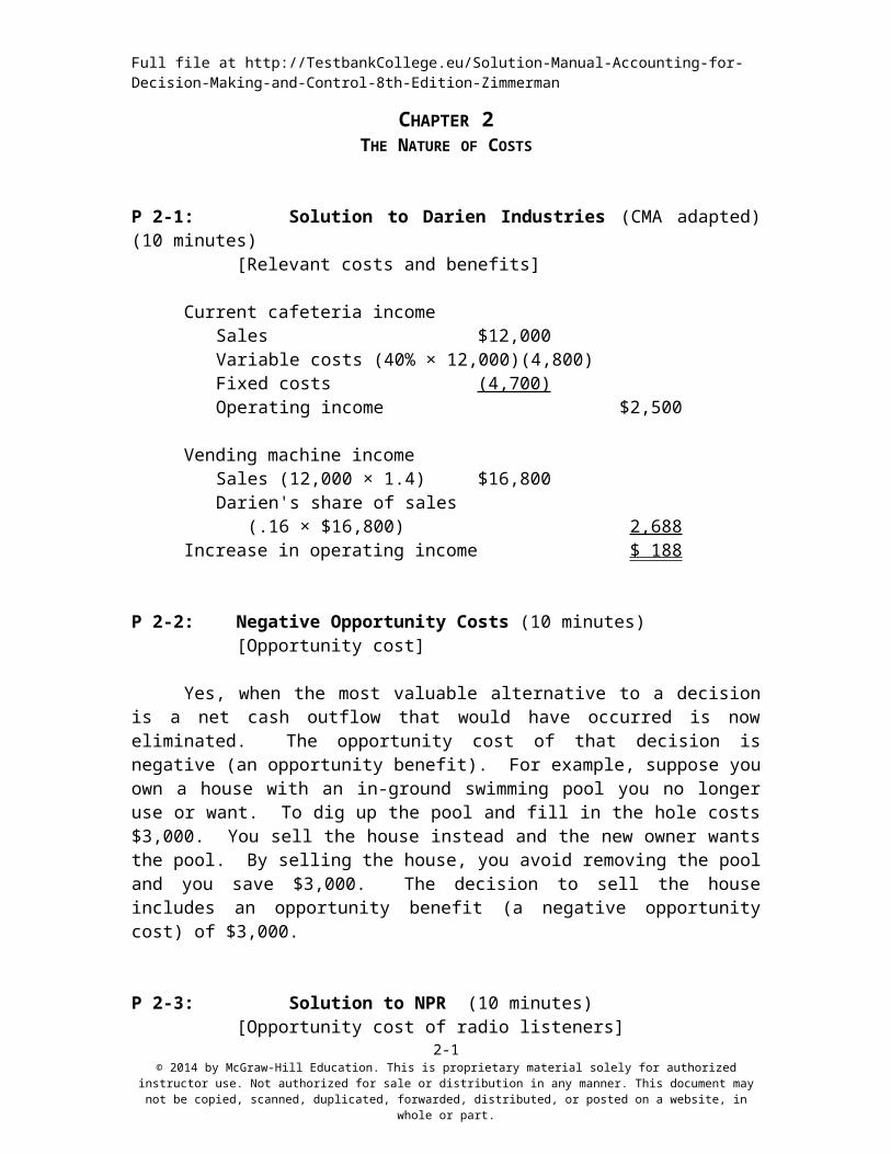
P 2-2: Negative Opportunity Costs (10 minutes)[Opportunity cost]
Yes, when the most valuable alternative to a decision is a net cash outflow that would have occurred is now eliminated. The opportunity cost of that decision is negative (an opportunity benefit). For example, suppose you own a house with an in-ground swimming pool you no longer use or want. To dig up the pool and fill in the hole costs $3,000. You sell the house instead and the new owner wants the pool. By selling the house, you avoid removing the pool and you save $3,000. The decision to sell the house includes an opportunity benefit (a negative opportunity cost) of $3,000.
P 2-3: Solution to NPR (10 minutes)[Opportunity cost of radio listeners]
The quoted passage ignores the opportunity cost of listeners’ having to forego normal programming for on-air pledges. While such fundraising campaigns may have a low out-of-pocket cost to NPR, if they were to consider the listeners’ opportunity cost, such campaigns may be quite costly.
distribution in any manner. This document may not be copied, scanned, duplicated, forwarded, distributed, or posted on a website, in whole or part.
Full file at http://TestbankCollege.eu/Solution-Manual-Accounting-for-Decision-Making-and-Control-8th-Edition-Zimmerman
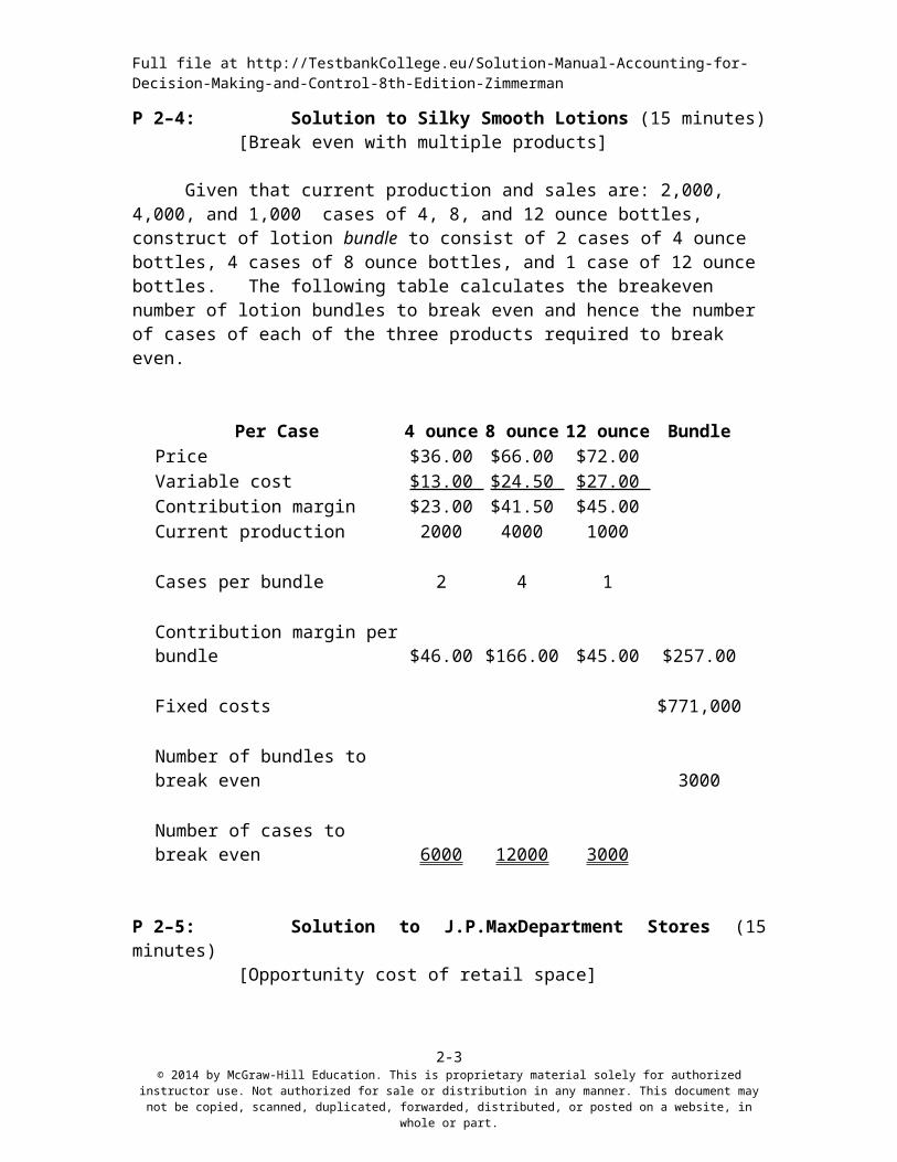
P 2–4: Solution to Silky Smooth Lotions (15 minutes)[Break even with multiple products]
Given that current production and sales are: 2,000, 4,000, and 1,000 cases of 4, 8, and 12 ounce bottles, construct of lotion bundle to consist of 2 cases of 4 ounce bottles, 4 cases of 8 ounce bottles, and 1 case of 12 ounce bottles. The following table calculates the breakeven number of lotion bundles to break even and hence the number of cases of each of the three products required to break even.
Per Case 4 ounce 8 ounce 12 ounce BundlePrice $36.00 $66.00 $72.00 Variable cost $13.00 $24.50 $27.00 Contribution margin $23.00 $41.50 $45.00 Current production 2000 4000 1000
Cases per bundle 2 4 1
Contribution margin per bundle $46.00 $166.00 $45.00 $257.00
Fixed costs $771,000
Number of bundles to break even 3000
Number of cases to break even 6000 12000 3000
P 2–5: Solution to J.P.MaxDepartment Stores (15 minutes)[Opportunity cost of retail space]
Home Appliances TelevisionsProfits after fixed cost allocations $64,000 $82,000Allocated fixed costs 7,000 8,400Profits before fixed cost allocations 71,000 90,400Lease Payments 72,000 86,400Forgone Profits – $1,000 $ 4,000
We would rent out the Home Appliance department, as lease rental receipts are more than the profits in the Home Appliance Department. On the other hand, profits generated by the Television Department are more than the lease rentals if leased out, so we continue running the TV Department. However, neither is being charged inventory holding costs, which could easily change the decision.
Also, one should examine externalities. What kind of merchandise is being sold in the leased store and will this increase or decrease overall traffic and hence sales in the other departments?
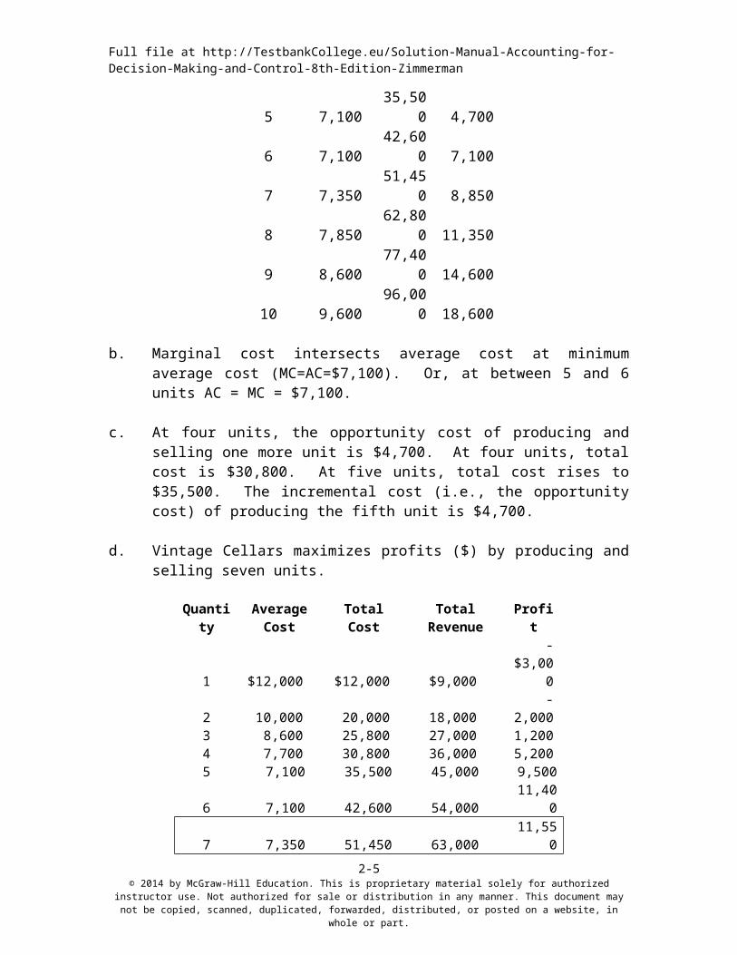
b. Marginal cost intersects average cost at minimum average cost (MC=AC=$7,100). Or, at between 5 and 6 units AC = MC = $7,100.
c. At four units, the opportunity cost of producing and selling one more unit is $4,700. At four units, total cost is $30,800. At five units, total cost rises to $35,500. The incremental cost (i.e., the opportunity cost) of producing the fifth unit is $4,700.
d. Vintage Cellars maximizes profits ($) by producing and selling seven units.
distribution in any manner. This document may not be copied, scanned, duplicated, forwarded, distributed, or posted on a website, in whole or part.
Full file at http://TestbankCollege.eu/Solution-Manual-Accounting-for-Decision-Making-and-Control-8th-Edition-Zimmerman
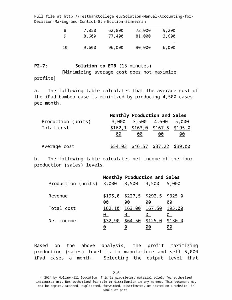
Monthly Production and SalesProduction (units) 3,000 3,500 4,500 5,000Total cost $162,100 $163,000 $167,500 $195,000
Average cost $54.03 $46.57 $37.22 $39.00
b. The following table calculates net income of the four production (sales) levels.
Monthly Production and SalesProduction (units) 3,000 3,500 4,500 5,000
Revenue $195,000 $227,500
$292,500 $325,000
Total cost 162,100 163,000 167,500 195,000 Net income
$32,900 $64,500$125,000 $130,000
Based on the above analysis, the profit maximizing production (sales) level is to manufacture and sell 5,000 iPad cases a month. Selecting the output level that minimizes average cost (4,500 cases) does not maximize profits.
P 2-8: Solution to Taylor Chemicals (15 minutes)[Relation between average, marginal, and total cost]
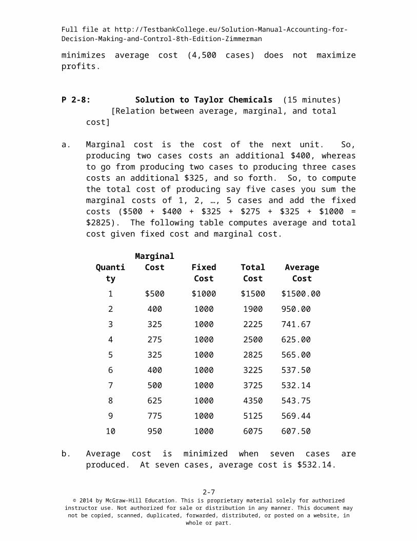
a. Marginal cost is the cost of the next unit. So, producing two cases costs an additional $400, whereas to go from producing two cases to producing three cases costs an additional $325, and so forth. So, to compute the total cost of producing say five cases you sum the marginal costs of 1, 2, …, 5 cases and add the fixed costs ($500 + $400 + $325 + $275 + $325 + $1000 = $2825). The following table computes average and total cost given fixed cost and marginal cost.
distribution in any manner. This document may not be copied, scanned, duplicated, forwarded, distributed, or posted on a website, in whole or part.
Full file at http://TestbankCollege.eu/Solution-Manual-Accounting-for-Decision-Making-and-Control-8th-Edition-Zimmerman
QuantityMarginal
CostFixedCost
TotalCost
AverageCost
1 $500 $1000 $1500 $1500.00
2 400 1000 1900 950.00
3 325 1000 2225 741.67
4 275 1000 2500 625.00
5 325 1000 2825 565.00
6 400 1000 3225 537.50
7 500 1000 3725 532.14
8 625 1000 4350 543.75
9 775 1000 5125 569.44
10 950 1000 6075 607.50
b. Average cost is minimized when seven cases are produced. At seven cases, average cost is $532.14.
c. Marginal cost always intersects average cost at minimum average cost. If marginal cost is above average cost, average cost is increasing. Likewise, when marginal cost is below average cost, average cost is falling. When marginal cost equals average cost, average cost is neither rising nor falling. This only occurs when average cost is at its lowest level (or at its maximum).
P 2-9: Solution to Emrich Processing (15 minutes)[Negative opportunity costs]
Opportunity costs are usually positive. In this case, opportunity costs are negative (opportunity benefits) because the firm can avoid disposal costs if they accept the rush job.
The original $1,000 price paid for GX-100 is a sunk cost. The opportunity cost of GX-100 is -$400. That is, Emrich will increase its cash flows by $400 by accepting the rush order because it will avoid having to dispose of the remaining GX-100 by paying Environ the $400 disposal fee.
How to price the special order is another question. Just because the $400 disposal fee was built into the previous job does not mean it is irrelevant in pricing this job. Clearly, one factor to consider in pricing this job is the reservation price of the customer proposing the rush order. The $400 disposal fee enters the pricing decision in the following way: Emrich should be prepared to pay up to $399 less any out-of-pocket costs to get this contract.
distribution in any manner. This document may not be copied, scanned, duplicated, forwarded, distributed, or posted on a website, in whole or part.
Full file at http://TestbankCollege.eu/Solution-Manual-Accounting-for-Decision-Making-and-Control-8th-Edition-Zimmerman
P 2–10: Solution to Gas Prices (15 minutes)[“Price gouging” or increased opportunity cost?]
The opportunity cost of the oil in process was higher after the invasion and thus the oil companies were justified in raising prices as quickly as they did. For example, suppose the oil company had one barrel of oil purchased at $15. This barrel was refined and processed for another $5 of cost and then the refined products from the barrel sold for $21. Replacing that barrelrequires the oil company to pay another $15 per barrel on top of the $15 per barrel it is already paying. Therefore, in order to replace the old barrel, the prices of the refined products must be raised as soon as the crude oil price rises.
However, accounting treats the realized holding gain on the old oil as an accounting profit, not as an opportunity cost. Therefore, the income statement of oil companies with large stocks of in-process crude will show accounting profits, unless they can somehow defer these profits. Switching to income-decreasing accounting methods and writing off obsolete equipment will help the oil companies avoid the political embarrassment of reporting the holding gains. In January 1990, the large oil companies received significant adverse media publicity when they reported large increases in fourth-quarter profits.
It is useful having discussed this problem to ask the following question: What happens to oil companies in the reverse situation when a large, unexpected price drop occurs? Suppose the oil company purchased old barrels for $15 and sold the refined products for $21. New barrels now can be purchased for $10. The company would like to keep selling refined products at $21, but competition from other oil companies will push the price of refined products down. Depending on how quickly the price of refined products fall, the oil companies will report smaller (maybe even negative) accounting earnings as their inventory of $15 oil gets refined and sold, but at lower prices.
P 2–11: Solution to Penury Company (15 minutes)[Break-even analysis with multiple products]
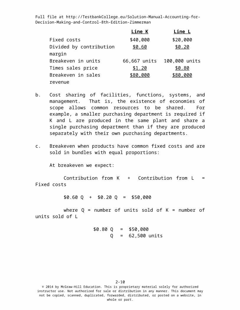
a. Breakeven when products have separate fixed costs:
Line K Line L
Fixed costs $40,000 $20,000Divided by contribution margin $0.60 $0.20Breakeven in units 66,667 units 100,000 unitsTimes sales price $1.20 $0.80Breakeven in sales revenue $80,000 $80,000
b. Cost sharing of facilities, functions, systems, and management. That is, the existence of economies of scope allows common resources to be shared. For example, a smaller purchasing department is required if K and L are produced in the same plant and share a single purchasing department than if they are produced separately with their own purchasing departments.
distribution in any manner. This document may not be copied, scanned, duplicated, forwarded, distributed, or posted on a website, in whole or part.
Full file at http://TestbankCollege.eu/Solution-Manual-Accounting-for-Decision-Making-and-Control-8th-Edition-Zimmerman
c. Breakeven when products have common fixed costs and are sold in bundles with equal proportions:
At breakeven we expect:
Contribution from K + Contribution from L = Fixed costs
$0.60 Q + $0.20 Q = $50,000
where Q = number of units sold of K = number of units sold of L
$0.80 Q = $50,000Q = 62,500 units
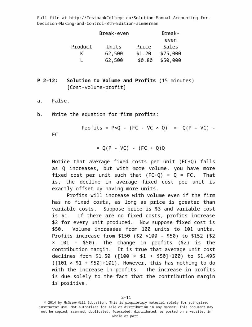
Break-even Break-evenProduct
KL
Units62,50062,500
Price$1.20 $0.80
Sales$75,000$50,000
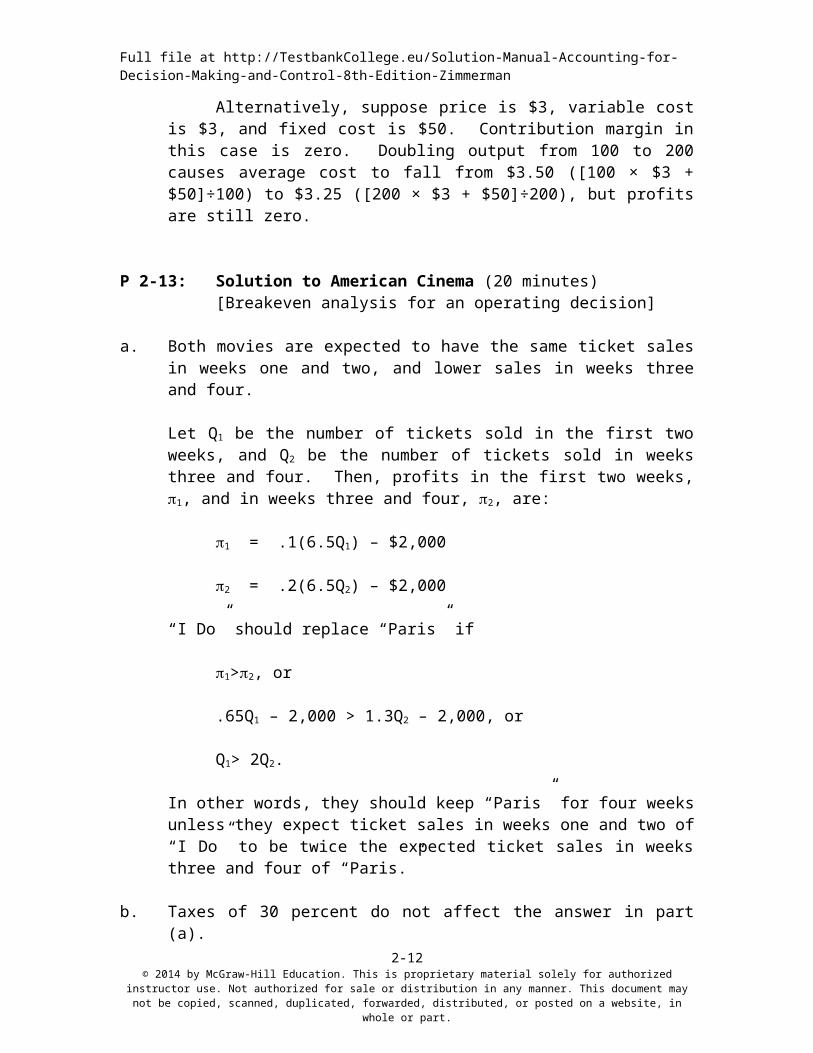
P 2–12: Solution to Volume and Profits (15 minutes)[Cost-volume-profit]
a. False.
b. Write the equation for firm profits:
Profits = P×Q - (FC - VC × Q) = Q(P - VC) - FC
= Q(P - VC) - (FC ÷ Q)Q
Notice that average fixed costs per unit (FC÷Q) falls as Q increases, but with more volume, you have more fixed cost per unit such that (FC÷Q) × Q = FC. That is, the decline in average fixed cost per unit is exactly offset by having more units.
Profits will increase with volume even if the firm has no fixed costs, as long as price is greater than variable costs. Suppose price is $3 and variable cost is $1. If there are no fixed costs, profits increase $2 for every unit produced. Now suppose fixed cost is $50. Volume increases from 100 units to 101 units. Profits increase from $150 ($2 ×100 - $50) to $152 ($2 × 101 - $50). The change in profits ($2) is the contribution margin. It is true that average unit cost declines from $1.50 ([100 × $1 + $50]÷100) to $1.495 ([101 × $1 + $50]÷101). However, this has nothing to do with the increase in profits. The increase in profits is due solely to the fact that the contribution margin is positive.
Alternatively, suppose price is $3, variable cost is $3, and fixed cost is $50. Contribution margin in this case is zero. Doubling output from 100 to 200
distribution in any manner. This document may not be copied, scanned, duplicated, forwarded, distributed, or posted on a website, in whole or part.
Full file at http://TestbankCollege.eu/Solution-Manual-Accounting-for-Decision-Making-and-Control-8th-Edition-Zimmerman
causes average cost to fall from $3.50 ([100 × $3 + $50]÷100) to $3.25 ([200 × $3 + $50]÷200), but profits are still zero.
P 2-13: Solution to American Cinema (20 minutes)[Breakeven analysis for an operating decision]
a. Both movies are expected to have the same ticket sales in weeks one and two, and lower sales in weeks three and four.
Let Q1 be the number of tickets sold in the first two weeks, and Q2 be the number of tickets sold in weeks three and four. Then, profits in the first two weeks, 1, and in weeks three and four, 2, are:
1 = .1(6.5Q1) – $2,000
2 = .2(6.5Q2) – $2,000
“I Do” should replace “Paris” if
1>2, or
.65Q1 – 2,000 > 1.3Q2 – 2,000, or
Q1> 2Q2.
In other words, they should keep “Paris” for four weeks unless they expect ticket sales in weeks one and two of “I Do” to be twice the expected ticket sales in weeks three and four of “Paris.”
b. Taxes of 30 percent do not affect the answer in part (a).
c. With average concession profits of $2 per ticket sold,
1 = .65Q1 + 2Q1 – 2,000
2 = 1.30Q2 + 2Q2 – 2,000
1>2 if
2.65Q1> 3.3Q2
Q1> 1.245Q2
Now, ticket sales in the first two weeks need only be about 25 percent higher than in weeks three and four to replace “Paris” with “I Do.”
distribution in any manner. This document may not be copied, scanned, duplicated, forwarded, distributed, or posted on a website, in whole or part.
Full file at http://TestbankCollege.eu/Solution-Manual-Accounting-for-Decision-Making-and-Control-8th-Edition-Zimmerman
P 2-14: Solution to Home Auto Parts (20 minutes)[Opportunity cost of retail display space]
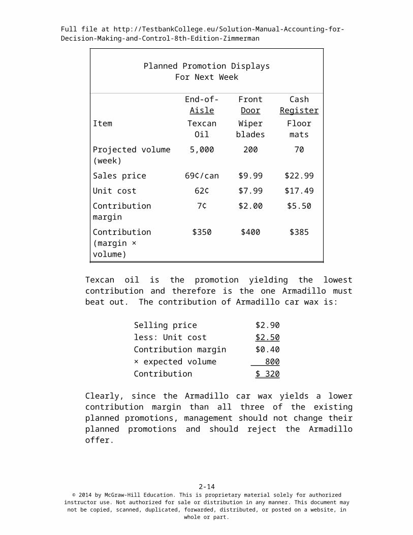
a. The question involves computing the opportunity cost of the special promotions being considered. If the car wax is substituted, what is the forgone profit from the dropped promotion? And which special promotion is dropped? Answering this question involves calculating the contribution of each planned promotion. The opportunity cost of dropping a planned promotion is its forgone contribution: (retail price less unit cost) × volume. The table below calculates the expected contribution of each of the three planned promotions.
Planned Promotion DisplaysFor Next Week
End-of-Aisle
FrontDoor
CashRegister
Item Texcan Oil Wiper blades Floor mats
Projected volume (week) 5,000 200 70
Sales price 69¢/can $9.99 $22.99
Unit cost 62¢ $7.99 $17.49
Contribution margin 7¢ $2.00 $5.50
Contribution(margin × volume)
$350 $400 $385
Texcan oil is the promotion yielding the lowest contribution and therefore is the one Armadillo must beat out. The contribution of Armadillo car wax is:
Clearly, since the Armadillo car wax yields a lower contribution margin than all three of the existing planned promotions, management should not change their planned promotions and should reject the Armadillo offer.
distribution in any manner. This document may not be copied, scanned, duplicated, forwarded, distributed, or posted on a website, in whole or part.
Full file at http://TestbankCollege.eu/Solution-Manual-Accounting-for-Decision-Making-and-Control-8th-Edition-Zimmerman
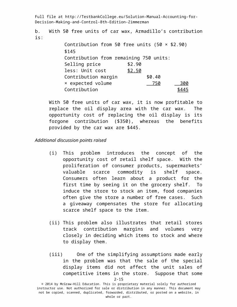
b. With 50 free units of car wax, Armadillo’s contribution is:Contribution from 50 free units (50 × $2.90) $145Contribution from remaining 750 units:Selling price $2.90less: Unit cost $2.50Contribution margin $0.40× expected volume 750 300Contribution $445
With 50 free units of car wax, it is now profitable to replace the oil display area with the car wax. The opportunity cost of replacing the oil display is its forgone contribution ($350), whereas the benefits provided by the car wax are $445.
Additional discussion points raised
(i) This problem introduces the concept of the opportunity cost of retail shelf space. With the proliferation of consumer products, supermarkets’ valuable scarce commodity is shelf space. Consumers often learn about a product for the first time by seeing it on the grocery shelf. To induce the store to stock an item, food companies often give the store a number of free cases. Such a giveaway compensates the store for allocating scarce shelf space to the item.
(ii) This problem also illustrates that retail stores track contribution margins and volumes very closely in deciding which items to stock and where to display them.
(iii) One of the simplifying assumptions made early in the problem was that the sale of the special display items did not affect the unit sales of competitive items in the store. Suppose that some of the Texcan oil sales came at the expense of other oil sales in the store. Discuss how this would alter the analysis.
P 2–15: Solution to Measer (20 minutes)[Average versus variable cost]
"Beware of unit costs." If you focus solely on the unit cost numbers in the problem, you are likely to be misled.
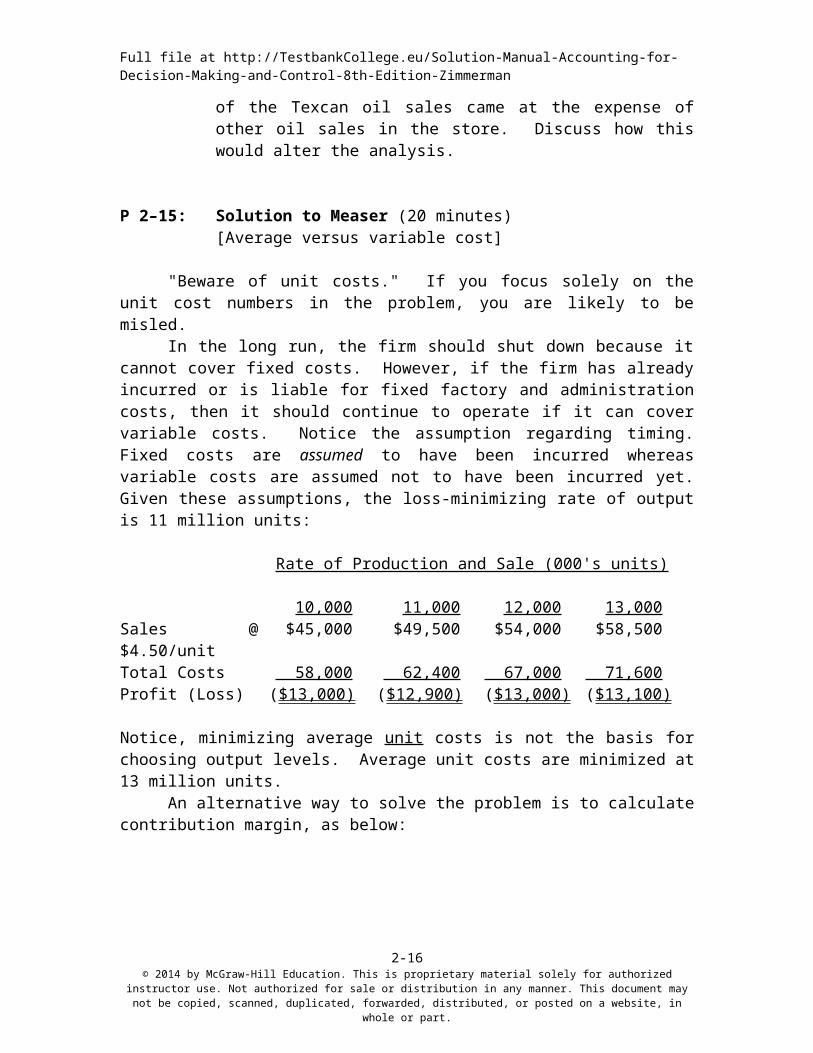
In the long run, the firm should shut down because it cannot cover fixed costs. However, if the firm has already incurred or is liable for fixed factory and administration costs, then it should continue to operate if it can cover variable costs. Notice the assumption regarding timing. Fixed costs are assumed to have been incurred whereas variable costs are assumed not to have been incurred yet. Given these assumptions, the loss-minimizing rate of output is 11 million units:
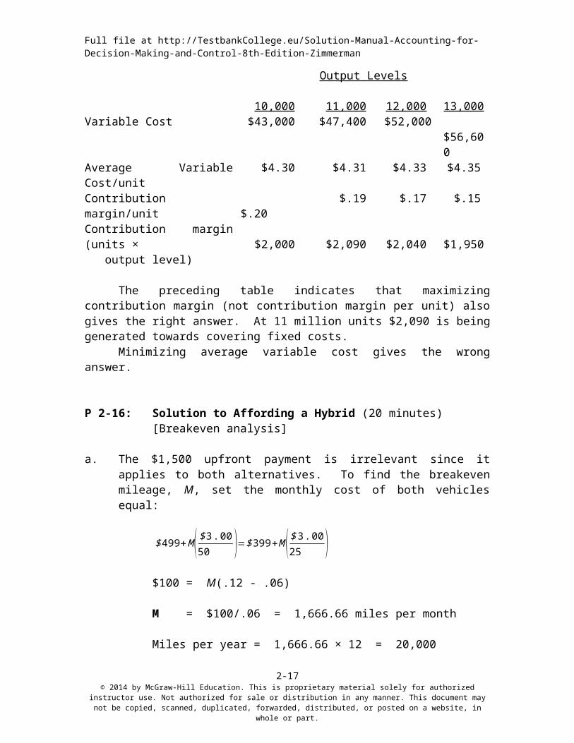
The preceding table indicates that maximizing contribution margin (not contribution margin per unit) also gives the right answer. At 11 million units $2,090 is being generated towards covering fixed costs.
Minimizing average variable cost gives the wrong answer.
P 2-16: Solution to Affording a Hybrid (20 minutes)[Breakeven analysis]
a. The $1,500 upfront payment is irrelevant since it applies to both alternatives. To find the breakeven mileage, M, set the monthly cost of both vehicles equal:
distribution in any manner. This document may not be copied, scanned, duplicated, forwarded, distributed, or posted on a website, in whole or part.
Full file at http://TestbankCollege.eu/Solution-Manual-Accounting-for-Decision-Making-and-Control-8th-Edition-Zimmerman
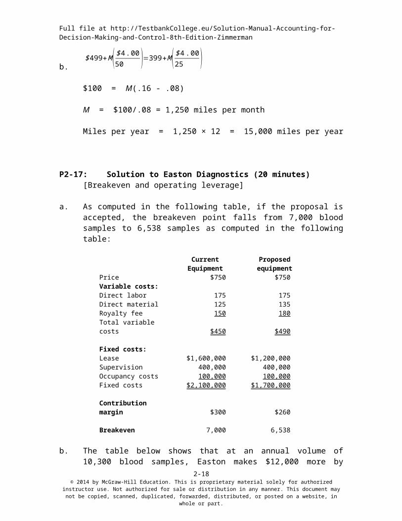
$100 = M(.16 - .08)
M = $100/.08 = 1,250 miles per month
Miles per year = 1,250 × 12 = 15,000 miles per year
P2-17: Solution to Easton Diagnostics (20 minutes)[Breakeven and operating leverage]
a. As computed in the following table, if the proposal is accepted, the breakeven point falls from 7,000 blood samples to 6,538 samples as computed in the following table:
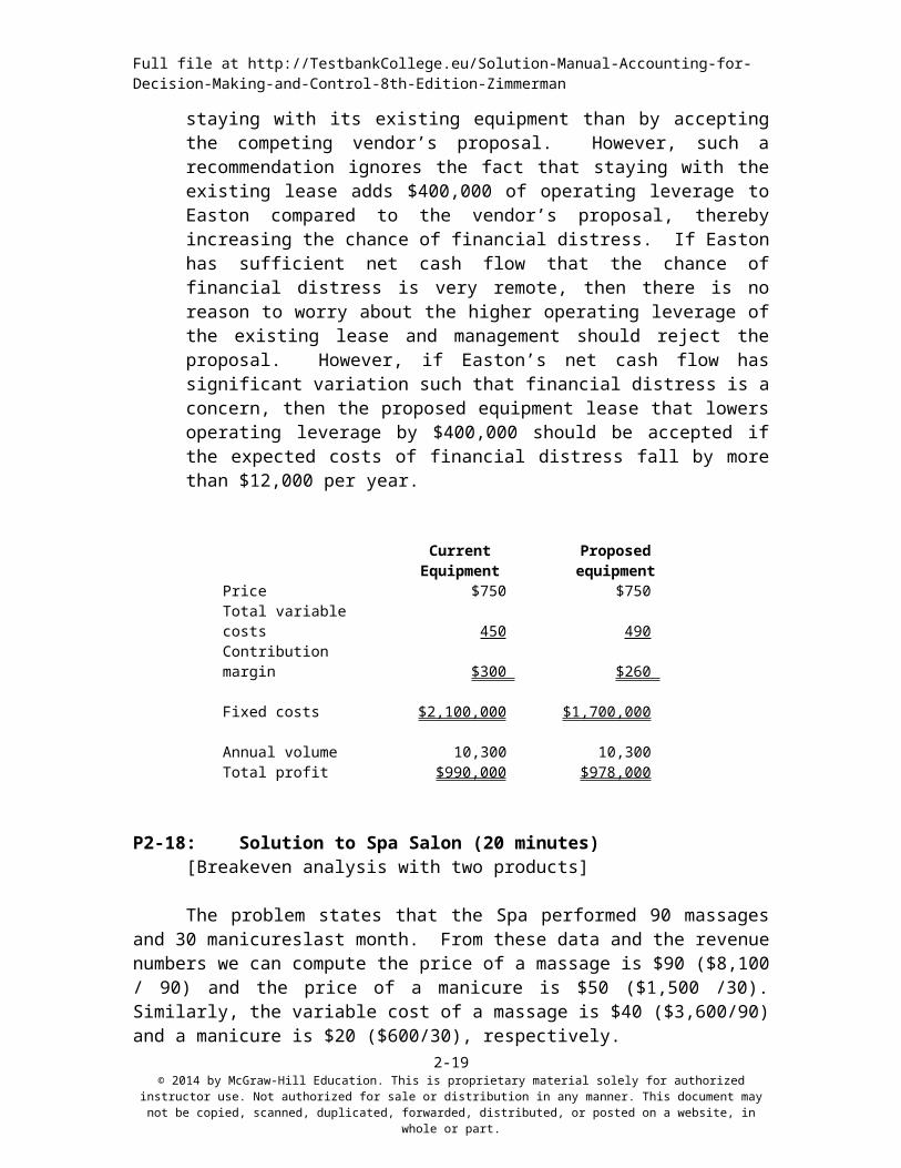
b. The table below shows that at an annual volume of 10,300 blood samples, Easton makes $12,000 more by staying with its existing equipment than by accepting the competing vendor’s proposal. However, such a recommendation ignores the fact that staying with the existing lease adds $400,000 of operating leverage to Easton compared to the vendor’s proposal, thereby increasing the chance of financial distress. If Easton has sufficient net cash flow that the chance of financial distress is very remote, then there is no reason to worry about the higher operating leverage of the existing lease and management should reject the proposal. However, if Easton’s net cash flow has significant variation such that financial distress is a concern, then the proposed equipment lease that lowers operating leverage by $400,000 should be accepted if the expected costs of financial distress fall by more than $12,000 per year.
P2-18: Solution to Spa Salon (20 minutes)[Breakeven analysis with two products]
The problem states that the Spa performed 90 massages and 30 manicureslast month. From these data and the revenue numbers we can compute the price of a massage is $90 ($8,100 / 90) and the price of a manicure is $50 ($1,500 /30). Similarly, the variable cost of a massage is $40 ($3,600/90) and a manicure is $20 ($600/30), respectively.
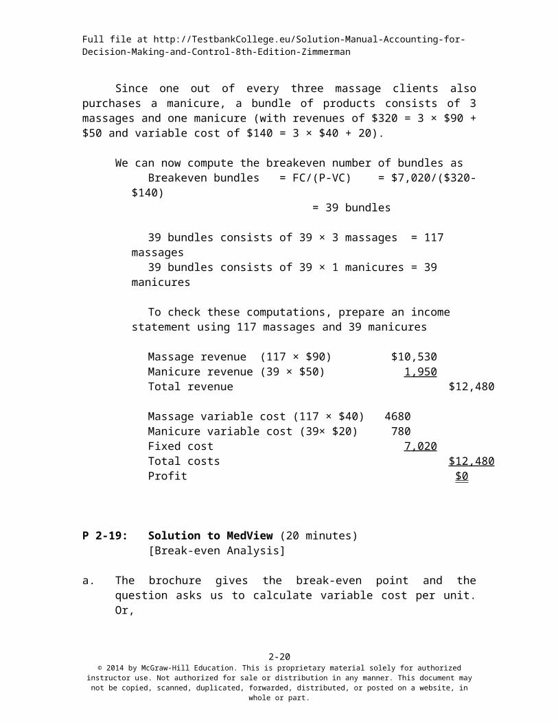
Since one out of every three massage clients also purchases a manicure, a bundle of products consists of 3 massages and one manicure (with revenues of $320 = 3 × $90 + $50 and variable cost of $140 = 3 × $40 + 20).
We can now compute the breakeven number of bundles as Breakeven bundles = FC/(P-VC) = $7,020/($320-$140)
distribution in any manner. This document may not be copied, scanned, duplicated, forwarded, distributed, or posted on a website, in whole or part.
Full file at http://TestbankCollege.eu/Solution-Manual-Accounting-for-Decision-Making-and-Control-8th-Edition-Zimmerman
P 2-19: Solution to MedView (20 minutes) [Break-even Analysis]
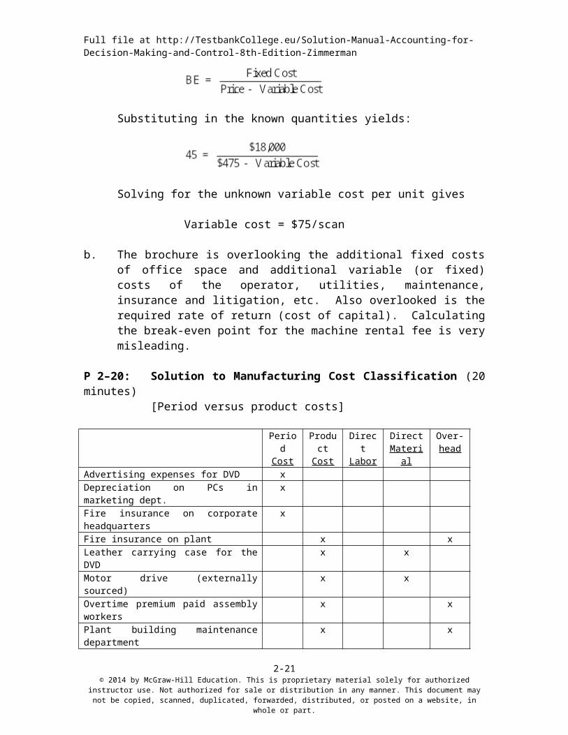
a. The brochure gives the break-even point and the question asks us to calculate variable cost per unit. Or,
Substituting in the known quantities yields:
Solving for the unknown variable cost per unit gives
Variable cost = $75/scan
b. The brochure is overlooking the additional fixed costs of office space and additional variable (or fixed) costs of the operator, utilities, maintenance, insurance and litigation, etc. Also overlooked is the required rate of return (cost of capital). Calculating the break-even point for the machine rental fee is very misleading.
P 2–20: Solution to Manufacturing Cost Classification (20 minutes)[Period versus product costs]
PeriodCost
ProductCost
DirectLabor
DirectMaterial
Over-head
Advertising expenses for DVD xDepreciation on PCs in marketing dept. xFire insurance on corporate headquarters xFire insurance on plant x xLeather carrying case for the DVD x xMotor drive (externally sourced) x xOvertime premium paid assembly workers x xPlant building maintenance department x xPlant security guards x xPlastic case for the DVD x xProperty taxes paid on corporate office xSalaries of public relations staff xSalary of corporate controller xWages of engineers in quality control dept. x xWages paid assembly line employees x xWages paid employees in finished goods warehouse
distribution in any manner. This document may not be copied, scanned, duplicated, forwarded, distributed, or posted on a website, in whole or part.
Full file at http://TestbankCollege.eu/Solution-Manual-Accounting-for-Decision-Making-and-Control-8th-Edition-Zimmerman
P 2–21: Solution to Australian Shipping (20 minutes)[Negative transportation costs]
a. Recommendation: The ship captain should be indifferent (at least financially) between using stone or wrought iron as ballast. The total cost (£550) is the same.
Stone as ballastCost of purchasing and loading stone £40Cost of unloading and disposing of stone 15
£55Ton required × 10Total cost £550
Wrought iron as ballastNumber of bars required:
10 tons of ballast × 2,000 pounds/ton 20,000 poundsWeight of bar ÷ 20 pounds/bar
1,000 bars
Loss per bar (£1.20 – £0.90) £0.30×number of bars 1,000
£300Cost of loading bars (£15 ×10) 150Cost of unloading bars (£10 ×10) 100Total cost £550
b. The price is lower in Sydney because the supply of wrought iron relative to demand is greater in Sydney because of wrought iron’s use as ballast. In fact, in equilibrium, ships will continue to import wrought iron as ballast as long as the relative price of wrought iron in London and Sydney make it cheaper (net of loading and unloading costs) than stone.
Contribution margin/impression $0.05 $0.03Breakeven number of impressions 300,000 166,667
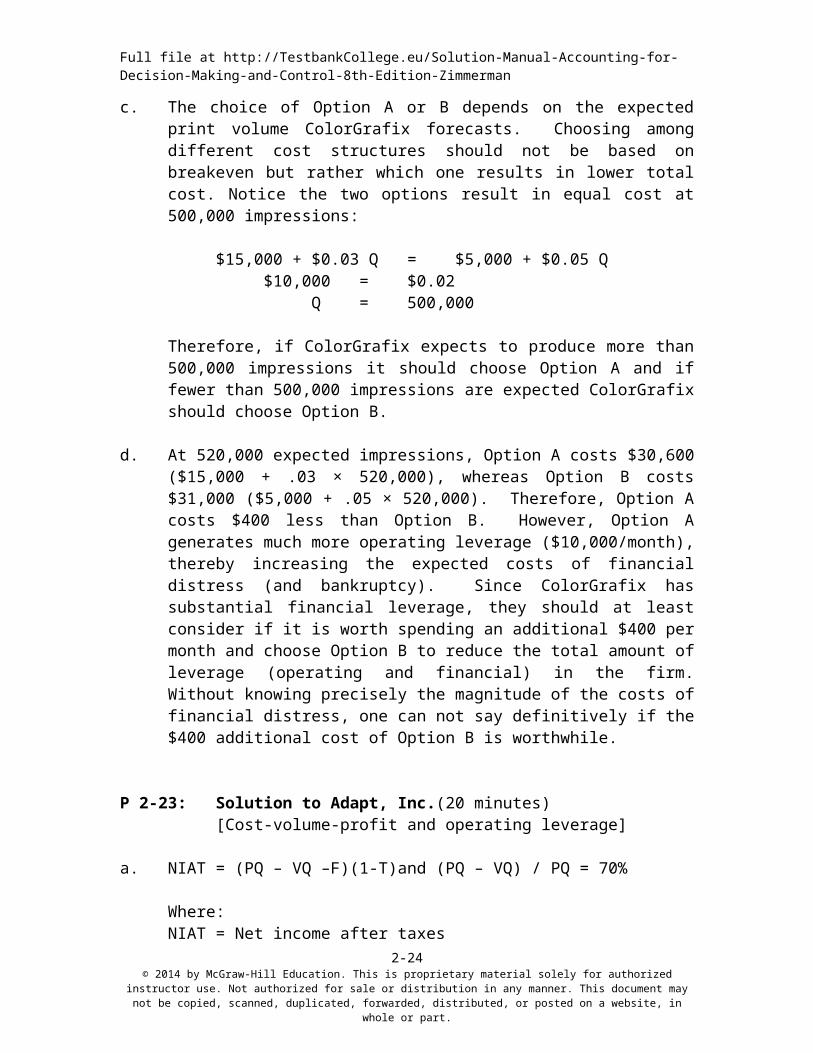
c. The choice of Option A or B depends on the expected print volume ColorGrafix forecasts. Choosing among different cost structures should not be based on breakeven but rather which one results in lower total cost. Notice the two options result in equal cost at 500,000 impressions:
Therefore, if ColorGrafix expects to produce more than 500,000 impressions it should choose Option A and if fewer than 500,000 impressions are expected ColorGrafix should choose Option B.
d. At 520,000 expected impressions, Option A costs $30,600 ($15,000 + .03 × 520,000), whereas Option B costs $31,000 ($5,000 + .05 × 520,000). Therefore, Option A costs $400 less than Option B. However, Option A generates much more operating leverage ($10,000/month), thereby increasing the expected costs of financial distress (and bankruptcy). Since ColorGrafix has substantial financial leverage, they should at least consider if it is worth spending an additional $400 per month and choose Option B to reduce the total amount of leverage (operating and financial) in the firm. Without knowing precisely the magnitude of the costs of financial distress, one can not say definitively if the $400 additional cost of Option B is worthwhile.
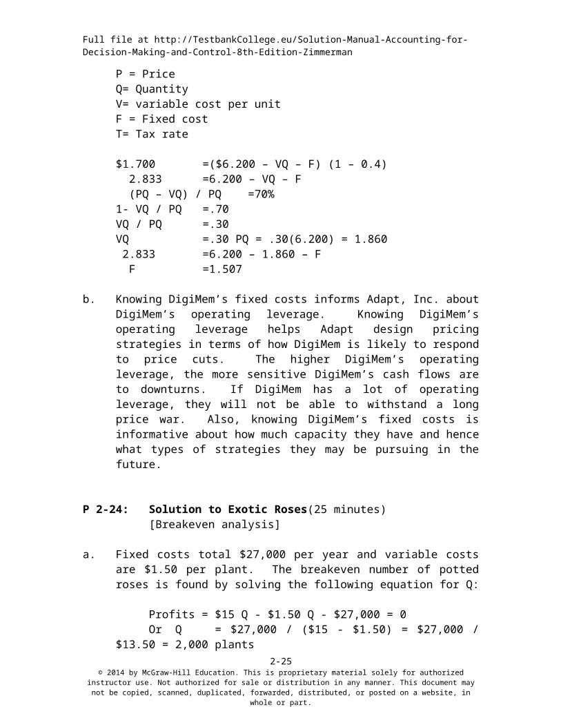
b. Knowing DigiMem’s fixed costs informs Adapt, Inc. about DigiMem’s operating leverage. Knowing DigiMem’s operating leverage helps Adapt design pricing strategies in terms of how DigiMem is likely to respond to price cuts. The higher DigiMem’s operating leverage, the more sensitive DigiMem’s cash flows are to downturns. If DigiMem has a lot of operating leverage, they will not be able to withstand a long price war. Also, knowing DigiMem’s fixed costs is informative about how much capacity they have and hence what types of strategies they may be pursuing in the future.
P 2-24: Solution to Exotic Roses(25 minutes)[Breakeven analysis]
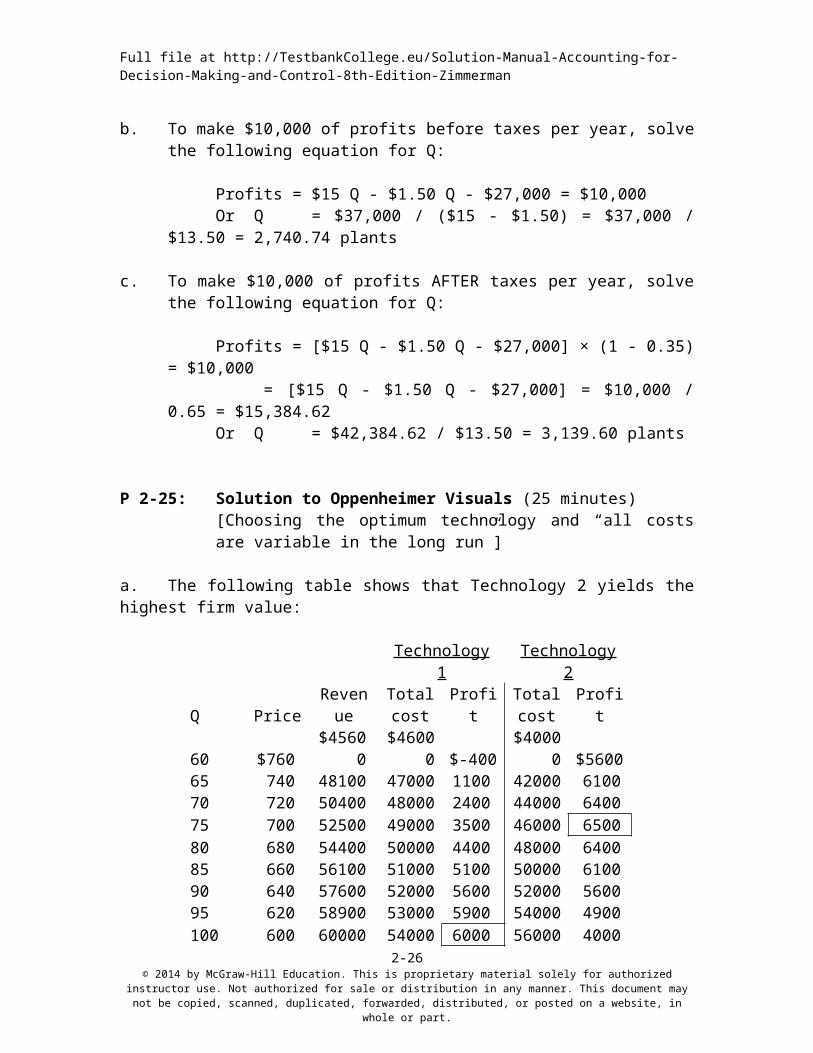
a. Fixed costs total $27,000 per year and variable costs are $1.50 per plant. The breakeven number of potted roses is found by solving the following equation for Q:
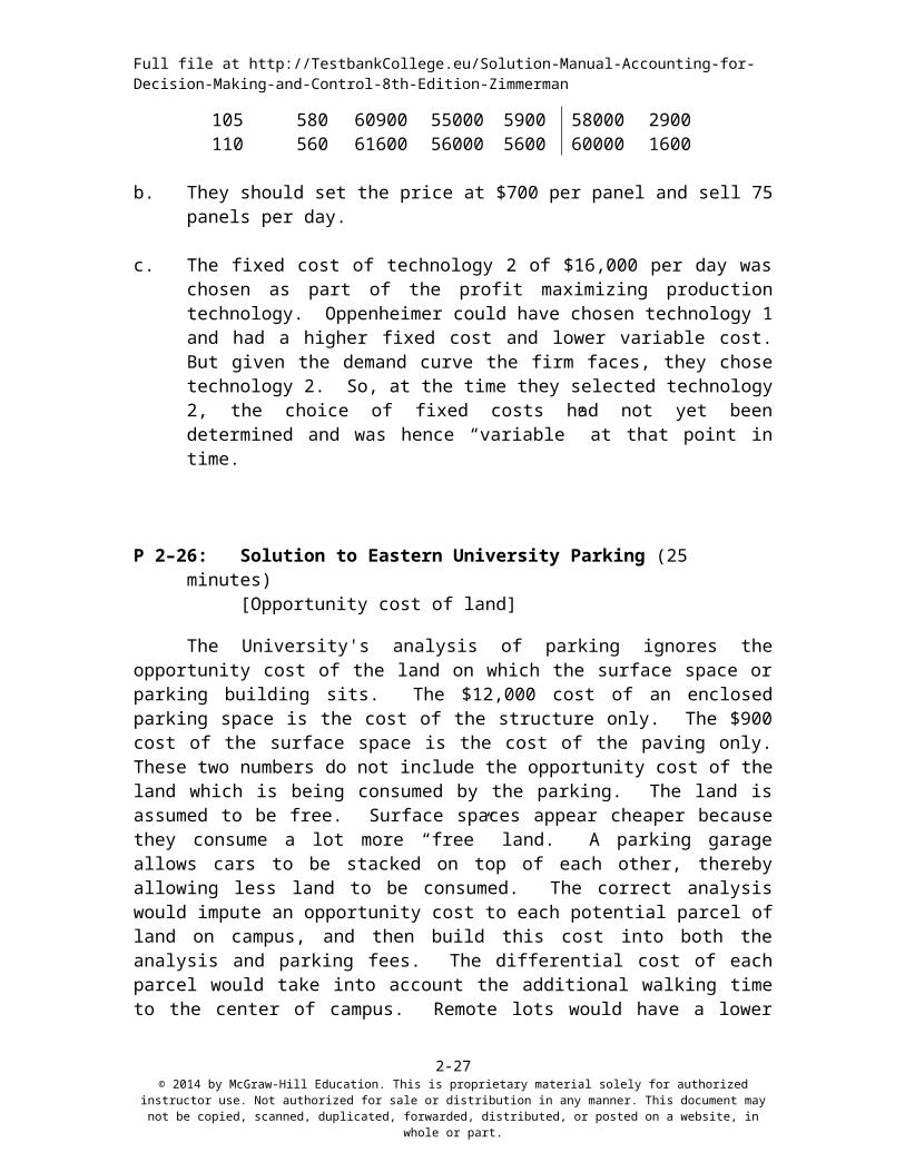
b. They should set the price at $700 per panel and sell 75 panels per day.
c. The fixed cost of technology 2 of $16,000 per day was chosen as part of the profit maximizing production technology. Oppenheimer could have chosen technology 1 and had a higher fixed cost and lower variable cost. But given the demand curve the firm faces, they chose technology 2. So, at the time they selected technology 2, the choice of fixed costs had not yet been determined and was hence “variable” at that point in time.
distribution in any manner. This document may not be copied, scanned, duplicated, forwarded, distributed, or posted on a website, in whole or part.
Full file at http://TestbankCollege.eu/Solution-Manual-Accounting-for-Decision-Making-and-Control-8th-Edition-Zimmerman
P 2–26: Solution to Eastern University Parking (25 minutes)[Opportunity cost of land]
The University's analysis of parking ignores the opportunity cost of the land on which the surface space or parking building sits. The $12,000 cost of an enclosed parking space is the cost of the structure only. The $900 cost of the surface space is the cost of the paving only. These two numbers do not include the opportunity cost of the land which is being consumed by the parking. The land is assumed to be free. Surface spaces appear cheaper because they consume a lot more “free” land. A parking garage allows cars to be stacked on top of each other, thereby allowing less land to be consumed. The correct analysis would impute an opportunity cost to each potential parcel of land on campus, and then build this cost into both the analysis and parking fees. The differential cost of each parcel would take into account the additional walking time to the center of campus. Remote lots would have a lower opportunity cost of land and would provide less expensive parking spaces.
Another major problem with the University's analysis is that parking prices should be set to allocate a scarce resource to those who value it the highest. If there is an excess demand for parking (i.e., queues exist), then prices should be raised to manage the queue and thereby allocate the scarce resource. Basing prices solely on costs does not guarantee that any excess supply or demand is eliminated.
Other relevant considerations in the decision to build a parking garage include:
1. The analysis ignores the effect of poor/inconvenient parking on tuition revenues.
2. Snow removal costs are likely lower, but other maintenance costs are likely to be higher with a parking garage.
The most interesting aspect of this question is "Why have University officials systematically overlooked the opportunity cost of the land in their decision-making process?" One implication of past University officials’ failure to correctly analyze the parking situation is the "dumb-administrator" hypothesis. Under this scenario, one concludes that all past University presidents were ignorant of the concept of opportunity cost and therefore failed to assign the "right" cost to the land.
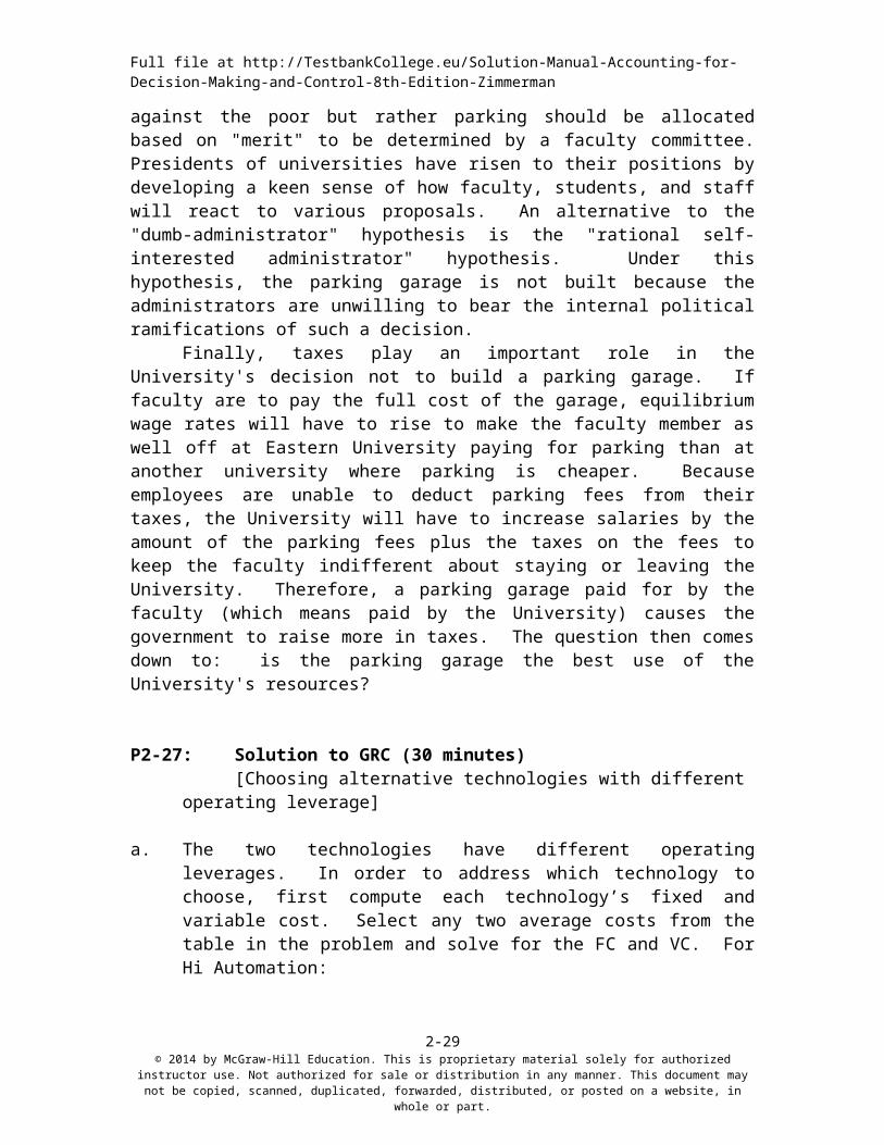
The way to understand why administrators will not build a parking garage is to ask what will happen if a garage is built and priced to recover cost. The cost of the covered space will be in excess of $1,200 per year. Those students, faculty, and staff with a high opportunity cost of their time (who tend to be those with higher incomes) will opt to pay the significantly higher parking fee for the garage. Lower-paid faculty will argue the inequity of allowing the "rich" the convenience of covered parking while the “poor” are relegated to surface lots. Arguments will undoubtedly be made by some constituents that parking spots should not be allocated using a price system which discriminates against the poor but rather parking should be allocated based on "merit" to be determined by a faculty committee. Presidents of universities have risen to their positions by developing a keen sense of how faculty, students, and staff will react to various proposals. An alternative to the "dumb-administrator" hypothesis is the "rational self-interested administrator" hypothesis. Under this hypothesis, the parking garage is
distribution in any manner. This document may not be copied, scanned, duplicated, forwarded, distributed, or posted on a website, in whole or part.
Full file at http://TestbankCollege.eu/Solution-Manual-Accounting-for-Decision-Making-and-Control-8th-Edition-Zimmerman
not built because the administrators are unwilling to bear the internal political ramifications of such a decision.
Finally, taxes play an important role in the University's decision not to build a parking garage. If faculty are to pay the full cost of the garage, equilibrium wage rates will have to rise to make the faculty member as well off at Eastern University paying for parking than at another university where parking is cheaper. Because employees are unable to deduct parking fees from their taxes, the University will have to increase salaries by the amount of the parking fees plus the taxes on the fees to keep the faculty indifferent about staying or leaving the University. Therefore, a parking garage paid for by the faculty (which means paid by the University) causes the government to raise more in taxes. The question then comes down to: is the parking garage the best use of the University's resources?
P2-27: Solution to GRC (30 minutes)[Choosing alternative technologies with different operating leverage]
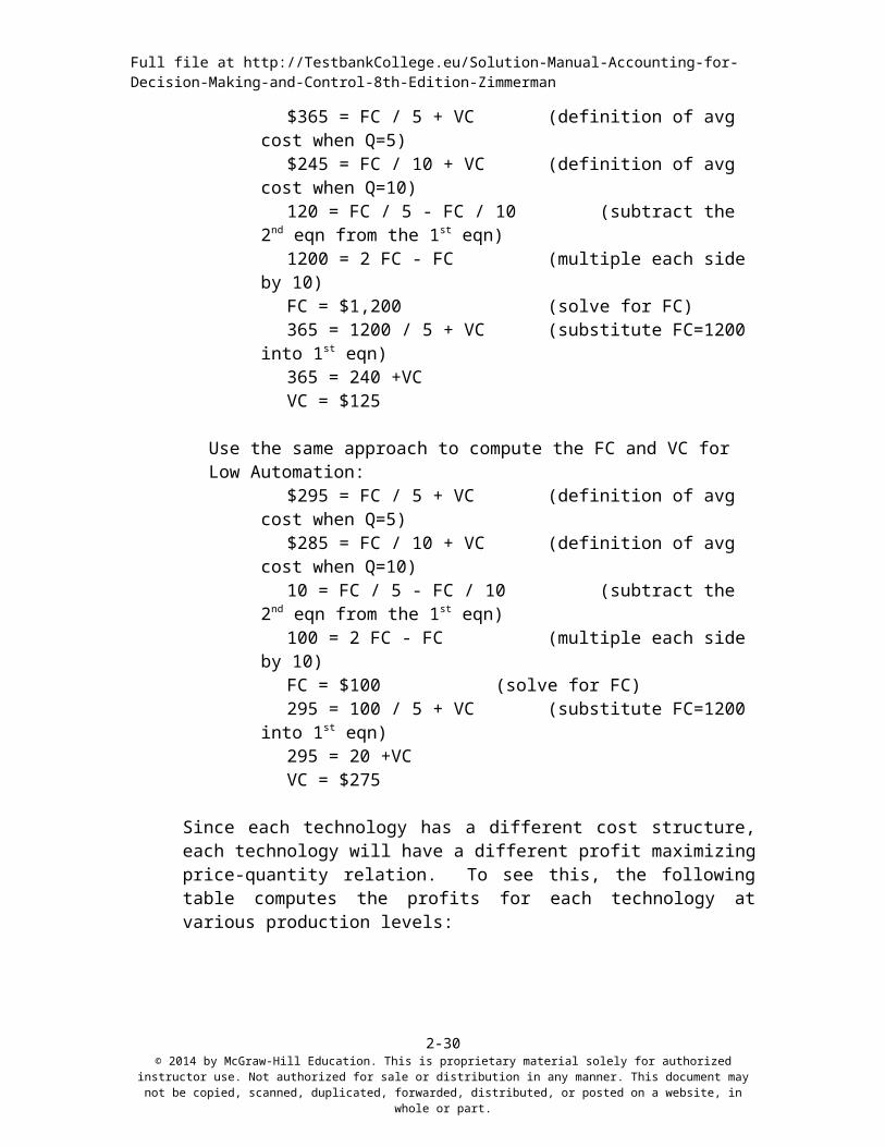
a. The two technologies have different operating leverages. In order to address which technology to choose, first compute each technology’s fixed and variable cost. Select any two average costs from the table in the problem and solve for the FC and VC. For Hi Automation:
$365 = FC / 5 + VC (definition of avg cost when Q=5)$245 = FC / 10 + VC (definition of avg cost when Q=10)120 = FC / 5 - FC / 10 (subtract the 2nd eqn from the 1st eqn)1200 = 2 FC - FC (multiple each side by 10)FC = $1,200 (solve for FC)365 = 1200 / 5 + VC (substitute FC=1200 into 1st eqn)365 = 240 +VCVC = $125
Use the same approach to compute the FC and VC for Low Automation:$295 = FC / 5 + VC (definition of avg cost when Q=5)$285 = FC / 10 + VC (definition of avg cost when Q=10)10 = FC / 5 - FC / 10 (subtract the 2nd eqn from the 1st eqn)100 = 2 FC - FC (multiple each side by 10)FC = $100 (solve for FC)295 = 100 / 5 + VC (substitute FC=1200 into 1st eqn)295 = 20 +VCVC = $275
Since each technology has a different cost structure, each technology will have a different profit maximizing price-quantity relation. To see this, the following table computes the profits for each technology at various production levels:
From this table, we see that if Hi Auto is chosen, it yields a maximum profit of $555,000 whereas if Low auto is chosen, it yields a maximum profit of $530,000. Hi Auto yields $25,000 more profit than Low Auto. In this simplified problem where there is no uncertainty, GRC should adopt the Hi Auto technology.
If there is substantial risk in this wind turbine venture (as there likely will be), then GRC should consider the Lo Auto option because it lowers GRC’s fixed cost structure, thereby reducing GRC’s operating risk. Less operating leverage, like lower financial leverage, reduces the expected costs of financial distress. Lowering profits by $25,000 via Low Auto may be a cheap way to reduce operating risk.
NOTE: If the demand curve is used instead of the table, the profit maximizing quantity for Hi Auto is 9.375 machines and 5.625 machines for Lo Auto. At these output levels, Hi Auto yields total profits of $557,813 and Lo Auto yields total profits of $532,813. The difference is still $25,000.
b. If Hi Auto is selected, then GRC should set the price of each gear machine at $320,000 and sell 9 machines per year. If Low Auto is selected, then GRC should set the price of each gear machine at $380,000 and sell 6 machines per year.NOTE: If the demand curve is used instead of the table, the profit maximizing
price for Hi Auto is $312,500 (500-20 x 9.375 machines) and $387,500 (500 - 20 x 5.625 machines) for Lo Auto.
P 2-28: Solution to Mastich Counters (25 minutes)[Opportunity cost to the firm of workers deferring vacation time]
At the core of this question is the opportunity cost of workers deferring vacation.The new policy was implemented because management believed it was costing
the firm too much money when workers left with accumulated vacation and were paid. However, these workers had given Mastich in effect a loan. By not taking their vacation time as accrued, they stayed in their jobs and worked, allowing Mastich to increase its
distribution in any manner. This document may not be copied, scanned, duplicated, forwarded, distributed, or posted on a website, in whole or part.
Full file at http://TestbankCollege.eu/Solution-Manual-Accounting-for-Decision-Making-and-Control-8th-Edition-Zimmerman
output without hiring additional workers, and without reducing output or quality. Mastich was able to produce more and higher quality output with fewer workers. Suppose a worker is paid $20 per hour this year and $20.60 next year. By deferring one vacation hour one year, the worker receives $20.60 when the vacation hour is taken next year. As long as average worker salary increases are less than the firm’s cost of capital, the firm is better off by workers accumulating vacation time. The firm receives a loan from its workers at less than the firm’s cost of capital.
Under the new policy, and especially during the phase-in period, Mastich has difficulty meeting production schedules and quality standards as more workers are now on vacation at any given time. To overcome these problems, the size of the work force will have to increase to meet the same production/quality standards. If the size of the work force stays the same, but more vacation time is taken, output/quality will fall.
Manager A remarked that workers were refreshed after being forced to take vacation. This is certainly an unintended benefit. But it also is a comment about how some supervisors are managing their people. If workers are burned out, why aren’t their supervisors detecting this and changing job assignments to prevent it? Moreover, how is burnout going to be resolved after the phase-in period is over and workers don’t have excess accumulated vacation time?
The new policy reduces the workers’ flexibility to accumulate vacation time, thereby reducing the attractiveness of Mastich as an employer. Everything else equal, workers will demand some offsetting form of compensation or else the quality of Mastich’s work force will fall.
Many of the proposed benefits, namely reducing costs, appear illusory. The opportunity costs of the new policy are reduced output, schedule delays, and possible quality problems. If workers under the new policy were forfeiting a significant number of vacation hours, these lost hours “profit” the firm. But, as expected from rational workers, very few vacation hours are being forfeited (as mentioned by Manager C).
However, there is one very real benefit of the new policy – less fraud and embezzlement. One key indicator of fraud used by auditors is an employee who never takes a vacation. Forced vacations mean other people have to cover the person’s job. During these periods, fraud and embezzlement often are discovered. Another benefit of this new policy is it reduces the time employees will spend lobbying their supervisors for extended vacations (in excess of three to four weeks). Finally, under the existing policy, employees tend to take longer average vacations (because workers have more accumulated vacation time). When a worker takes a long vacation, it is more likely the employee’s department will hire a temporary or “float” person to fill in. With shorter vacations, the work of the person on vacation is performed by the remaining employees. Thus, the new policy reduces the slack (free time) of the work force and results in higher productivity.
distribution in any manner. This document may not be copied, scanned, duplicated, forwarded, distributed, or posted on a website, in whole or part.
Full file at http://TestbankCollege.eu/Solution-Manual-Accounting-for-Decision-Making-and-Control-8th-Edition-Zimmerman
P 2-29: Solution to Optometry Practice (25 minutes)[Break-even analysis]
Hiring the optometrist generates two income streams, examination revenue and eyeglass and contact sales. Each exam is expected to produce the following additional revenue:
Frequency(1)
Profits(2)
Expected Profits(1) ×(2)
Eyeglasses 60% $90 $54Contact lens 20% $65 $13Expected Profits from sales per exam $67
The break-even point is calculated as follows:
Contribution margin per exam:Exam fee $ 45Expected gross margin on sales $ 67Contribution margin $112
distribution in any manner. This document may not be copied, scanned, duplicated, forwarded, distributed, or posted on a website, in whole or part.
Full file at http://TestbankCollege.eu/Solution-Manual-Accounting-for-Decision-Making-and-Control-8th-Edition-Zimmerman
P 2–30: Solution to JLE Electronics (25 minutes)[Maximize contribution margin per unit of scarce resource]
Notice that the new line has a maximum capacity of 25,200 minutes (21 ×20 × 60) which is less than the time required to process all four orders. The profit maximizing production schedule occurs when JLE selects those boards that have the largest contribution margin per minute of assembly time. The following table provides the calculations:
CUSTOMERSA B C D
Price $38 $42 $45 $50 Variable cost per unit 23 25 27 30Contribution margin $15 $17 $18 $20
Number of machine minutes 3 4 5 6Contribution margin/minute 5 4.25 3.6 3.33
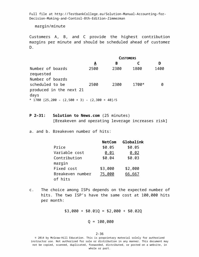
Customers A, B, and C provide the highest contribution margins per minute and should be scheduled ahead of customer D.
CUSTOMERSA B C D
Number of boards requested 2500 2300 1800 1400Number of boards scheduled to be produced in the next 21 days 2500 2300 1700* 0* 1700 [25,200 – (2,500 × 3) – (2,300 × 40]/5
P 2–31: Solution to News.com (25 minutes)[Breakeven and operating leverage increases risk]
a. and b. Breakeven number of hits:
NetCom GlobalinkPrice $0.05 $0.05Variable cost 0.01 0.02Contribution margin $0.04 $0.03Fixed cost $3,000 $2,000Breakeven number of hits 75,000 66,667
c. The choice among ISPs depends on the expected number of hits. The two ISP’s have the same cost at 100,000 hits per month:
distribution in any manner. This document may not be copied, scanned, duplicated, forwarded, distributed, or posted on a website, in whole or part.
Full file at http://TestbankCollege.eu/Solution-Manual-Accounting-for-Decision-Making-and-Control-8th-Edition-Zimmerman
Q = 100,000
If the number of hits exceeds 100,000 per month, NetCom is cheaper. If the number of hits is less than 100,000, Globalink is cheaper.
d. If demand fluctuates with general economy-wide factors, then the risk of News.com is not diversifiable and the variance (and covariance) of the two ISP’s will affect News.com’s risk. For example, the table below calculates News.com’s profits if they use NetCom or Globalink and demand is either high or low. Notice that News.com has the same expected profits ($1,000 per month) from using either ISP. However, the variance of profits (and hence risk) is higher under Net.Com than under Globalink. Therefore, News.com should hire Globalink. Basically, with lower fixed costs, but higher variable costs per hit, News.com’s profits don’t fluctuate as much with Globalink as they do with Net.Com.
P 2–32: Solution to Kinsley & Sons (25 minutes)[Opportunity cost of cannibalized sales]
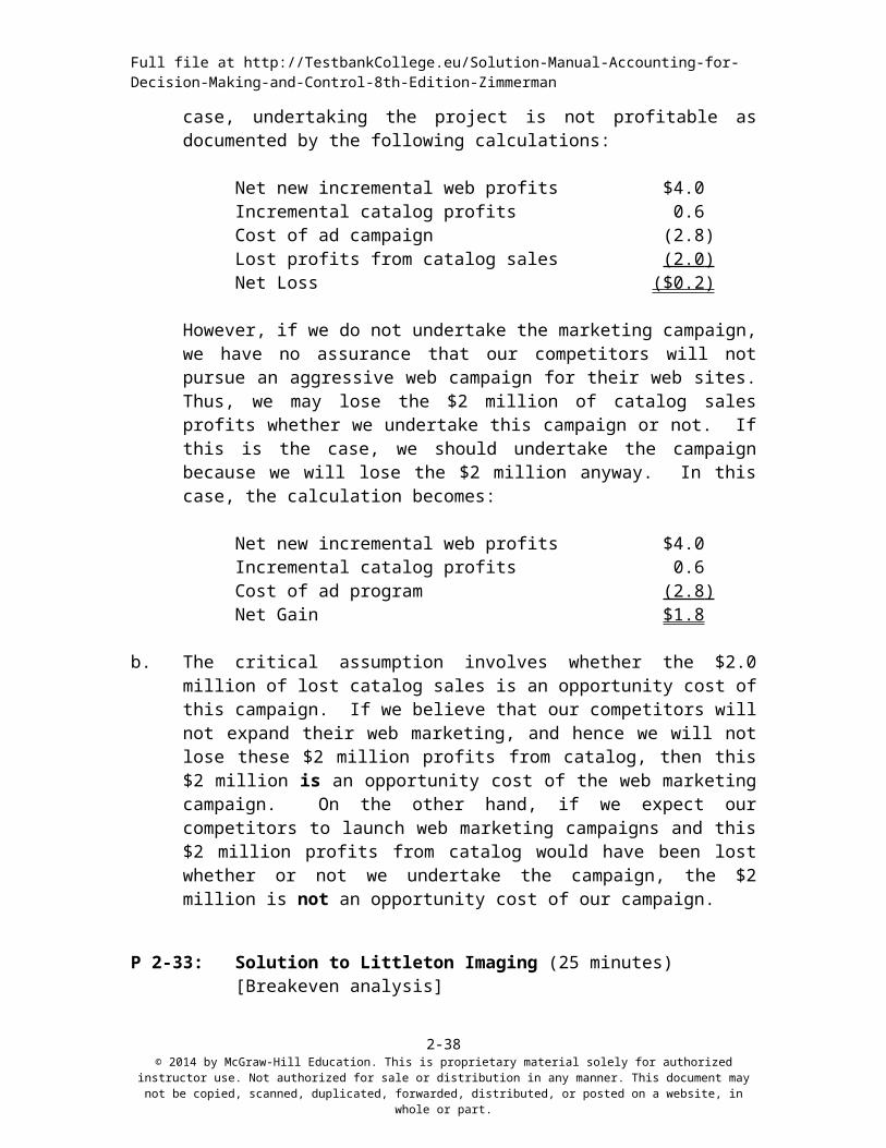
a. The decision to undertake the additional advertising and marketing campaign depends on how one considers the cannibalized sales from catalog. Additional web profits from the program will be $4 million. But half of these will be from existing catalog purchases. Thus, the net new profits are only $2 million. In this case, undertaking the project is not profitable as documented by the following calculations:
Net new incremental web profits $4.0Incremental catalog profits 0.6Cost of ad campaign (2.8)Lost profits from catalog sales (2 .0) Net Loss ($0 .2)
However, if we do not undertake the marketing campaign, we have no assurance that our competitors will not pursue an aggressive web campaign for their web sites. Thus, we may lose the $2 million of catalog sales profits whether we undertake this campaign or not. If this is the case, we should undertake the campaign because we will lose the $2 million anyway. In this case, the calculation becomes:
distribution in any manner. This document may not be copied, scanned, duplicated, forwarded, distributed, or posted on a website, in whole or part.
Full file at http://TestbankCollege.eu/Solution-Manual-Accounting-for-Decision-Making-and-Control-8th-Edition-Zimmerman
Net new incremental web profits $4.0Incremental catalog profits 0.6Cost of ad program (2 .8) Net Gain $1 .8
b. The critical assumption involves whether the $2.0 million of lost catalog sales is an opportunity cost of this campaign. If we believe that our competitors will not expand their web marketing, and hence we will not lose these $2 million profits from catalog, then this $2 million is an opportunity cost of the web marketing campaign. On the other hand, if we expect our competitors to launch web marketing campaigns and this $2 million profits from catalog would have been lost whether or not we undertake the campaign, the $2 million is not an opportunity cost of our campaign.
P 2-33: Solution to Littleton Imaging (25 minutes)[Breakeven analysis]
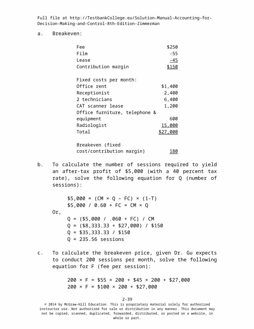
b. To calculate the number of sessions required to yield an after-tax profit of $5,000 (with a 40 percent tax rate), solve the following equation for Q (number of sessions):
$5,000 = (CM × Q – FC) × (1-T)$5,000 / 0.60 + FC = CM × Q
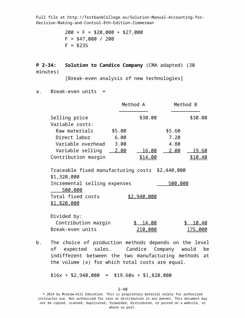
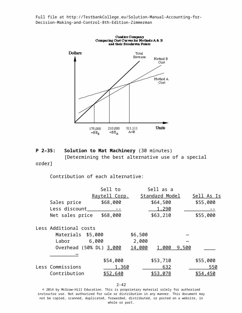
b. The choice of production methods depends on the level of expected sales. Candice Company would be indifferent between the two manufacturing methods at the volume (x) for which total costs are equal.
distribution in any manner. This document may not be copied, scanned, duplicated, forwarded, distributed, or posted on a website, in whole or part.
Full file at http://TestbankCollege.eu/Solution-Manual-Accounting-for-Decision-Making-and-Control-8th-Edition-Zimmerman
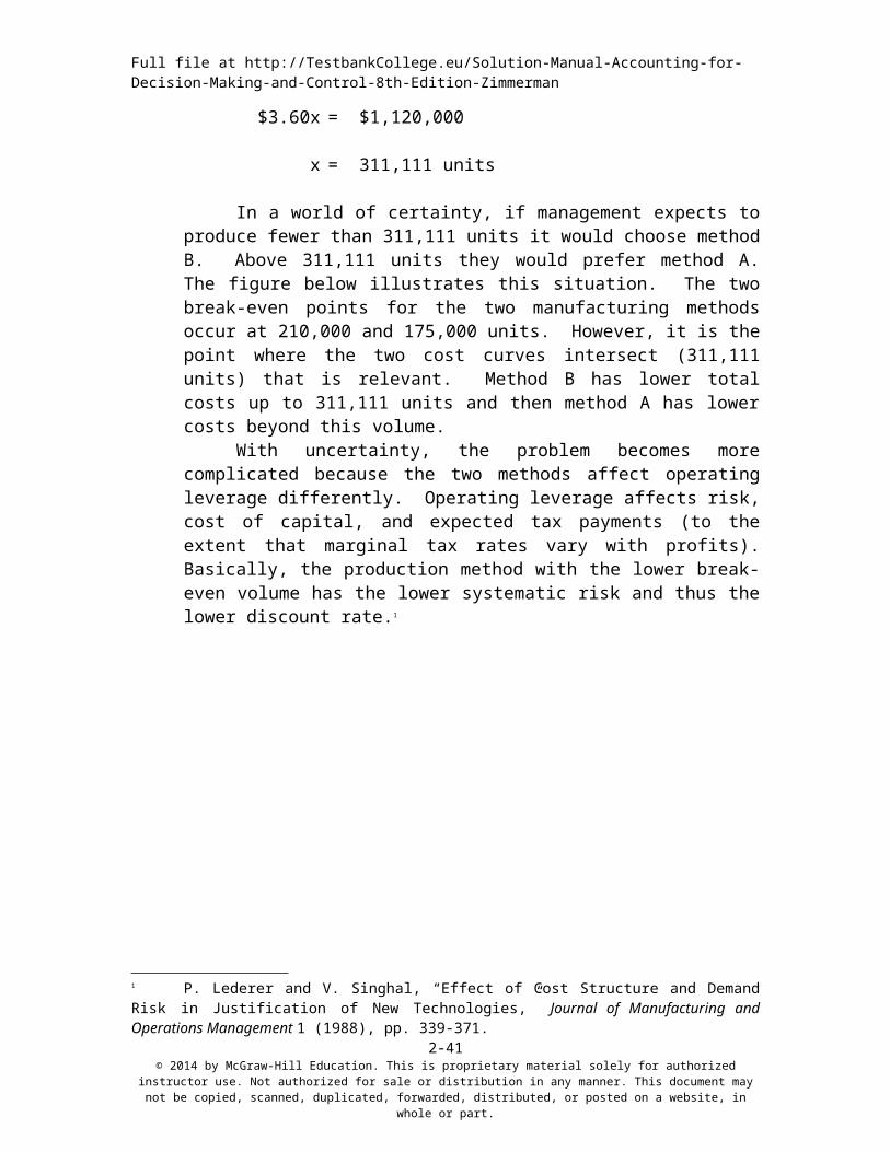
In a world of certainty, if management expects to produce fewer than 311,111 units it would choose method B. Above 311,111 units they would prefer method A. The figure below illustrates this situation. The two break-even points for the two manufacturing methods occur at 210,000 and 175,000 units. However, it is the point where the two cost curves intersect (311,111 units) that is relevant. Method B has lower total costs up to 311,111 units and then method A has lower costs beyond this volume.
With uncertainty, the problem becomes more complicated because the two methods affect operating leverage differently. Operating leverage affects risk, cost of capital, and expected tax payments (to the extent that marginal tax rates vary with profits). Basically, the production method with the lower break-even volume has the lower systematic risk and thus the lower discount rate.1
P 2–35: Solution to Mat Machinery (30 minutes)[Determining the best alternative use of a special order]
Contribution of each alternative:
1 P. Lederer and V. Singhal, “Effect of Cost Structure and Demand Risk in Justification of New Technologies,” Journal of Manufacturing and Operations Management 1 (1988), pp. 339-371.
Therefore, the “sell as is” for $55,000 is the best alternative. Notice that fixed factory overhead does not enter the analysis, as these costs are not relevant to any of the alternatives.
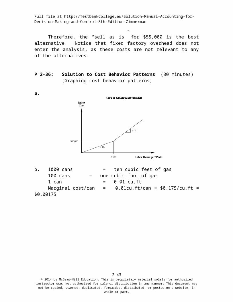
P 2-36: Solution to Cost Behavior Patterns (30 minutes)[Graphing cost behavior patterns]
a.
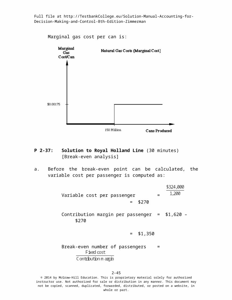
b. 1000 cans = ten cubic feet of gas100 cans = one cubic foot of gas1 can = 0.01 cu.ftMarginal cost/can = 0.01cu.ft/can × $0.175/cu.ft = $0.00175
distribution in any manner. This document may not be copied, scanned, duplicated, forwarded, distributed, or posted on a website, in whole or part.
Full file at http://TestbankCollege.eu/Solution-Manual-Accounting-for-Decision-Making-and-Control-8th-Edition-Zimmerman
b. The cost of the ship itself is not included. The weekly opportunity cost of the Mediterranean cruise is not using the ship elsewhere. One alternative use is to sell the ship and invest the proceeds. Since no other information is provided regarding alternative uses of the ship and assuming there are no capital gains taxes on the sale proceeds, the weekly opportunity cost of the ship is:
Sales proceeds $371,250,000×Interest rate 10%
$37,125,000÷ number of weeks/year 50Weekly opportunity cost $ 742,500
c. The revised break-even including the cost of the ship:
Total fixed costs = $607,500 + 742,500= $1,350,000
Break-even = = 1,000 passengers
d. Let C = contribution margin from additional sales
900 =
900(1,350 + C) = 1,350,000
900C = 1,350,000 – 1,350 ×900
C =
C = $150
Additional purchases per passenger = = $300.
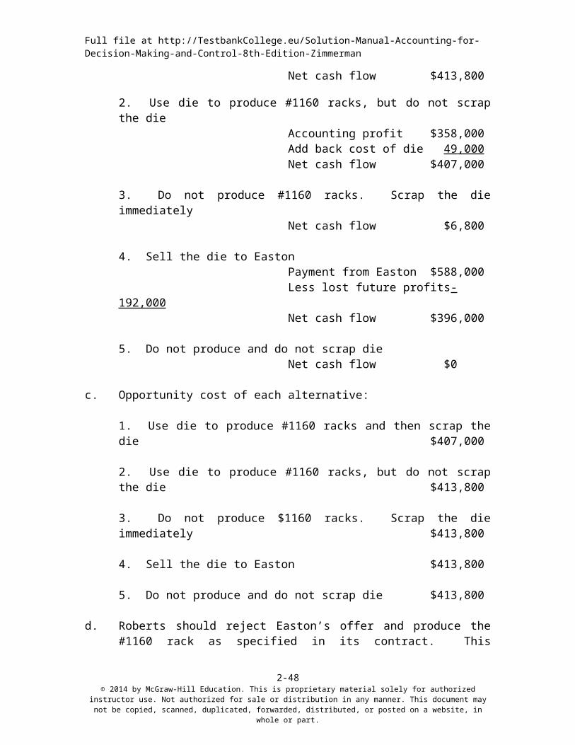
P 2–38: Solution to Roberts Machining (30 minutes)[Describing the opportunity set and determining opportunity costs]
a. The opportunity set consists of:
1. Use die to produce #1160 racks and then scrap the die.
distribution in any manner. This document may not be copied, scanned, duplicated, forwarded, distributed, or posted on a website, in whole or part.
Full file at http://TestbankCollege.eu/Solution-Manual-Accounting-for-Decision-Making-and-Control-8th-Edition-Zimmerman
2. Use die to produce #1160 racks, but do not scrap the die.3. Do not produce #1160 racks. Scrap the die immediately.4. Sell the die to Easton.5. Do not produce and do not scrap die.
b. Cash flows of each alternative (assuming GTE does not sue Roberts for breaching contract and ignoring discounting):
1. Use die to produce #1160 racks and then scrap the dieAccounting profit $358,000Add back cost of die 49,000Scrap 6,800Net cash flow $413,800
2. Use die to produce #1160 racks, but do not scrap the dieAccounting profit $358,000Add back cost of die 49,000Net cash flow $407,000
3. Do not produce #1160 racks. Scrap the die immediatelyNet cash flow $6,800
4. Sell the die to EastonPayment from Easton $588,000Less lost future profits -192,000Net cash flow $396,000
5. Do not produce and do not scrap dieNet cash flow $0
c. Opportunity cost of each alternative:
1. Use die to produce #1160 racks and then scrap the die $407,000
2. Use die to produce #1160 racks, but do not scrap the die $413,800
3. Do not produce $1160 racks. Scrap the die immediately $413,800
4. Sell the die to Easton $413,800
5. Do not produce and do not scrap die $413,800
d. Roberts should reject Easton’s offer and produce the #1160 rack as specified in its contract. This alternative has the lowest opportunity cost (or equivalently, it has the greatest net cash flow).
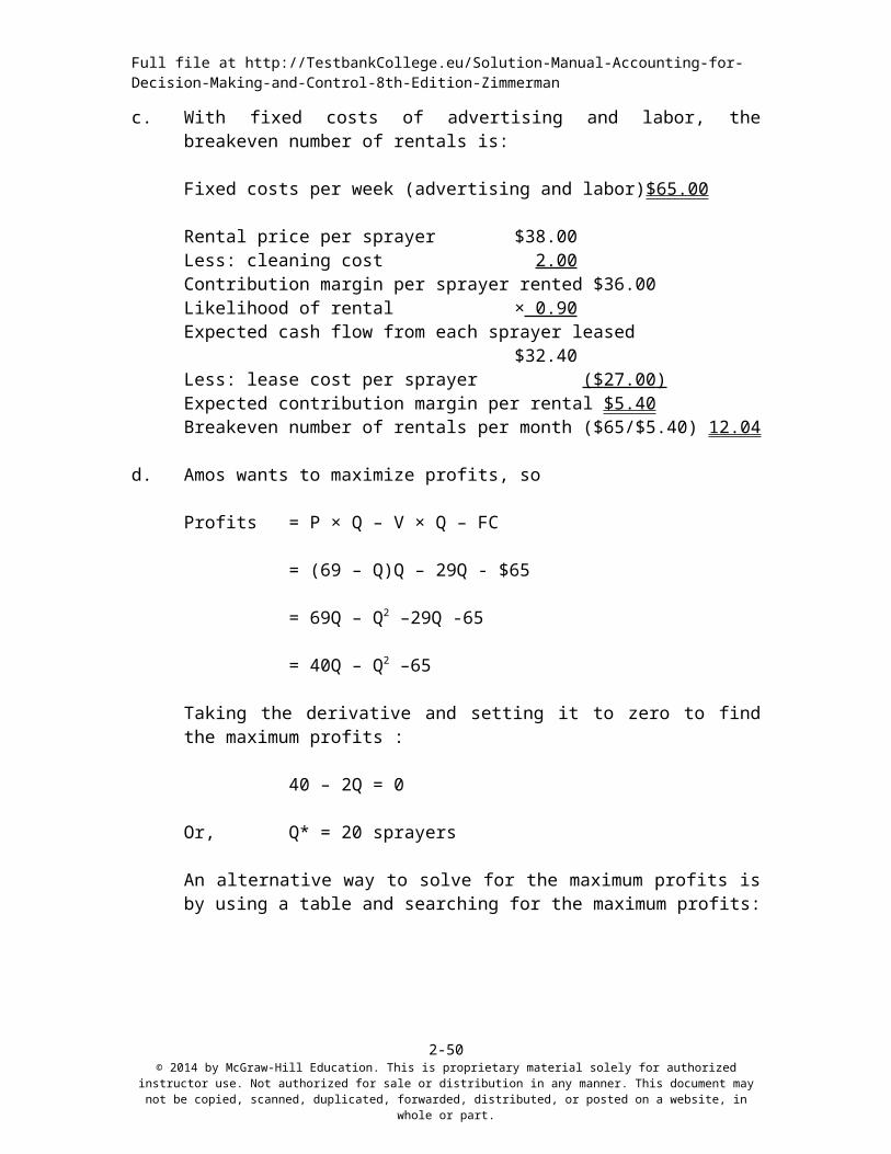
b. No, Amos is ignoring the opportunity cost of his time spent leasing and renting the sprayers. He could be spending this time marketing his other rentals. He should also consider the additional rentals of his other items (punch bowls) from customers coming into his store to rent sprayers as a potential benefit of the sprayers.
c. With fixed costs of advertising and labor, the breakeven number of rentals is:
Fixed costs per week (advertising and labor) $65 .00
Rental price per sprayer $38.00Less: cleaning cost 2 .00 Contribution margin per sprayer rented $36.00Likelihood of rental × 0 .90 Expected cash flow from each sprayer leased $32.40Less: lease cost per sprayer ($27 .00) Expected contribution margin per rental $5 .40 Breakeven number of rentals per month ($65/$5.40) 12 .04
b. With 70 hours (or 4200 minutes) of capacity per week, all the products can be manufactured. However, since only 200 cases of KY662 are ordered and KY662 has a breakeven quantity of 300 cases, KY662 should not be produced even though there is excess capacity (4200 minutes).
Fuller AerosolsMinutes on the Fill Line to Produce All Products
AA143 AC747 CD887 FX881 HF324 KY662Total
MinutesFill time per case (minutes) 3 4 5 2 3 4Cases ordered 300 100 50 200 400 200Minutes 900 400 250 400 1200 800 3950
An aerosol product should only be produced if its contribution margin times the number of units sold exceeds its fixed costs.
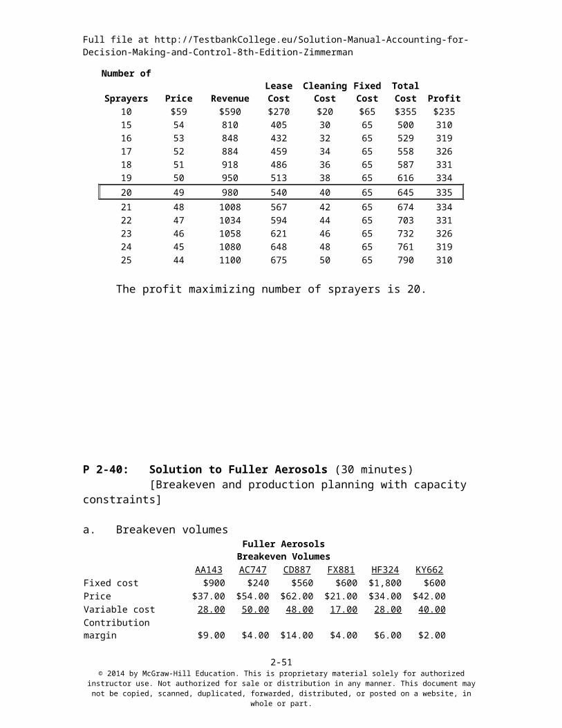
c. Given a capacity constraint on the aerosol fill line, products should be produced that maximize total profits (including the fixed costs). The following table lists the order in which the products should be produced and the quantity of each produced. Products AA143, AC747, FX881, and HF324 are produced to meet demand. After producing these four products to meet demand, 100 minutes remain to produce 20 cases out of the 100 cases ordered of CD887. Making 20 cases of CD887 is below CD887’s breakeven volume of 40 cases, so no CD887 should be produced. And KY662 is not produced because it does not cover its fixed costs at the number of cases demanded (200). The following table derives the solution.
distribution in any manner. This document may not be copied, scanned, duplicated, forwarded, distributed, or posted on a website, in whole or part.
Full file at http://TestbankCollege.eu/Solution-Manual-Accounting-for-Decision-Making-and-Control-8th-Edition-Zimmerman
Fuller AerosolsProduction Schedule with Only 3,000 Minutes (50 hours × 60 minutes/hour) of Fill Line Time
AA143 AC747 CD887 FX881 HF324 KY662Minutes
AvailableFill time per case (minutes) 3 4 5 2 3 4Cases ordered 300 100 50 200 400 200Minutes 900 400 250 400 1200 800Profit (loss) (from part a) $1,800 $160 $140 $200 $600 -$200Most to least profitable product 1 4 5 3 2 6Total minutes available 3,000Minutes used to meet demand for AA143 900 2,100Minutes used to meet demand forHF324 1200 900Minutes used to meet demand for FX881 400 500Minutes used to meet demand for AC747 400 100Minutes available to meet demand for CD887 100 100Cases of CD887 that can be manufactured 20Breakeven volume 100 60 40 150 300 300Cases manufactured 300 100 0 200 400 0
[Acknowledgement: I thank Nick Ripstein, a student at Concordia University, Nebraska and Professor Stan Obermueller for providing a corrected version of the solution].
P 2-41: Solution to Happy Feet (30 minutes)[Breakeven and operating leverage]
a. Breakeven sales is calculated using the following formula:
Profits = 0 = Revenues – cost of goods sold – fixed costs
0 = R – 0.5R - $63,000 - .03R
0.47 = $63,000
R = $134,042.55
b. Dr. Zang should probably accept the revised lease agreement. The following table shows that she actually makes less money ($750 per month) at her expected sales level of $150,000 per month if she accepts the revised rental agreement of $1,000 per month plus 12.5 percent of sales. However, the revised lease agreement reduces her risk of bankruptcy.
distribution in any manner. This document may not be copied, scanned, duplicated, forwarded, distributed, or posted on a website, in whole or part.
Full file at http://TestbankCollege.eu/Solution-Manual-Accounting-for-Decision-Making-and-Control-8th-Edition-Zimmerman
+ 3%Lease
+ 12.5%Lease
Revenues $150,000 $150,000Cost of goods sold 75,000 75,000Fixed rent 13,333 1,000Lease fee as % of sales 4,500 18,750Interest on bank loan 11,667 10,500Other costs 38,000 38,000Profits $7,500 $6,750
Note that depreciation on the store improvements are excluded from the calculation of profits since we are really interested in looking at cash flows from the business. Besides, depreciation is the same under both lease agreements, and hence does not affect the decision.
The slightly lower profit of $750 per month is a fairly low price to pay to lower the venture’s operating leverage by making the landlord a pseudo partner in Happy Feet. The following table illustrates the effect on profits if revenues fluctuate between Dr. Zang’s $80,000 and $220,000 estimates.
$13,333+ 3% Lease
$1,000+ 12.5% Lease
Revenues $80,000 $220,000 $80,000 $220,000Cost of goods sold 40,000 110,000 40,000 110,000Fixed rent 13,333 13,333 1,000 1,000Lease fee % of sales 2,400 6,600 10,000 27,500Interest on bank loan 11,667 11,667 10,500 10,500Other costs 38,000 38,000 38,000 38,000Profits -$25,400 $40,400 -$19,500 $33,000
Here we see that if sales are only $80,000, the revised lease results in a smaller loss (-$19,500) than under the original lease (-$25,400). If sales are $220,000, the store generates $7,400 more under the original lease than the revised lease. But given Dr. Zang’s limited working capital, the roughly $5,000 smaller loss when sales are low could be important, especially if there are a number of months of low sales until the store becomes established. Moreover, if the sales are substantially above Dr. Zang’s estimates, the lease can be renegotiated in three years.
P 2-42: Solution to Digital Convert(30 minutes)[Operating leverage and the cost of financial distress]
b. If DC adopts the new technology, profits are maximized at a wholesale price of $1,050 and a quantity of 25 units as calculated in the following table:
c. The following table shows that adopting the new sensor manufacturing technology does not maximize DC’s total profits after considering the expected cost of financial distress. Adopting the new technology lowers the value of DC by $12,800. In other words, DC should stay with its current manufacturing technology.
Monthly profits from the new technology $16,750Monthly profits from the existing technology 15,200Incremental profits from the new technology $1,550Number of months the new technology must be leased ×24Incremental profits over the next 24 months $37,200
Cost of financial distress $500,000Increase in likelihood of financial distress over 24 months ×10 % Increase in expected cost of financial distress $50,000
distribution in any manner. This document may not be copied, scanned, duplicated, forwarded, distributed, or posted on a website, in whole or part.
Full file at http://TestbankCollege.eu/Solution-Manual-Accounting-for-Decision-Making-and-Control-8th-Edition-Zimmerman
Expected total profits (loss) of new technology ($12,800 )
P 2-43: Solution to APC Electronics (35 minutes)[Accounting versus opportunity cost]
a. The hourly cost of operating each of the four lines is calculate in the following table:
LINE I LINE II LINE III LINE IVEquipment depreciation $840,000 $1,300,000 $480,000 $950,000Occupancy costs 213,000 261,000 189,000 237,000Total annual line costs $1,053,000 $1,561,000 $669,000 $1,187,000Expected hours of operations 1,800 2,200 1,600 2,000Operating cost per hour $585.00 $709.55 $418.13 $593.50
b. If APC accepts this special order from Healthtronics, APC will record cost of goods sold of:
distribution in any manner. This document may not be copied, scanned, duplicated, forwarded, distributed, or posted on a website, in whole or part.
Full file at http://TestbankCollege.eu/Solution-Manual-Accounting-for-Decision-Making-and-Control-8th-Edition-Zimmerman
Number of technicians 3 Hours during the evening 16 Cost per hour $42 2,016SonarTech:Tear-down time Hours 2 Cost per hour $40 80Set-up labor Hours 6 Cost per hour $40 240Overtime costs Number of technicians 4 Hours 14 Overtime rate ($14/hour) $14 784Additional Freight 2,300Total cost $6,756
P 2-44: Solution to Amy’s Boards (35 minutes)[Break-even analysis — short-run versus long-run]
The major goals of this problem are to demonstrate how fixed costs first become fixed and second to illustrate the relation between fixed costs and capacity. Before the snow boards are purchased in part (a), they are a variable cost. (In the long run, all costs are variable.) However, once purchased, the boards are a fixed cost. The number of boards purchased determines the shop’s total capacity, which is fixed, until she either buys more boards or sells used boards.
a. Number of boards to break-even:Fixed Costs
Store rent (net of sublet, $7,200 - $1,600) $ 5,600Salaries, advertising, office expense 26,000
$31,600Contribution margin per board per year:
Revenue per week $75Refurbishing cost -7Contribution margin per board per week $68×number of weeks 20Seasonal contribution margin from 100% rental $1,360
×likelihood of rental 80%Expected seasonal contribution margin per board $1,088Net cost per board ($550 – $250) 300Net contribution per board per year $788
Break-even number of boards ($31,600 ÷ $788) 40 .10
distribution in any manner. This document may not be copied, scanned, duplicated, forwarded, distributed, or posted on a website, in whole or part.
Full file at http://TestbankCollege.eu/Solution-Manual-Accounting-for-Decision-Making-and-Control-8th-Edition-Zimmerman
b. Expected profit with 50 boards:Expected seasonal contribution margin per board (from part a) $1,088
×number of boards 50Expected contribution margin $54,400Less:
Cost of boards ($300 ×50) (15,000)Fixed costs (31,600)
Expected profit $ 7,800
c. Break-even number of rentals with 50 boards:Total fixed costs
Store rent $ 5,600Salaries, advertising, and office expense 26,000Boards and boots (net of resale, $300 ×50) 15,000
$46,600
Contribution margin per board per week $68
Break-even number of rentals 685.29
Total possible number of rentals (50 boards ×20 weeks) 1,000
Break-even fraction of boards rented each week 68.5%
d. In the long run, all costs are variable. However, once purchased, the boards are a fixed cost. The reason for the difference is Amy has about ten more boards than the break-even number calculated in part (a). In part (a), before the boards are purchased, they are a variable cost. She can buy any number of boards she wants and pay a proportionately higher cost for them and rent them all 80 percent of the time. Therefore the cost of the boards is a variable cost with respect to the number of rentals. It is subtracted from the revenue in calculating the contribution margin per board. Once you buy the boards, their cost becomes fixed. Instead of being included in calculating contribution margin, it is included in the fixed cost (numerator of the breakeven volume).
b. Profits are maximized when the price is set at $310 and 1,100 boards are sold.
c. If fixed costs fall from $70,000 to $50,000, prices should not be changed because a price of $310 and 1,100 boards continue to maximize profits as illustrated below:
distribution in any manner. This document may not be copied, scanned, duplicated, forwarded, distributed, or posted on a website, in whole or part.
Full file at http://TestbankCollege.eu/Solution-Manual-Accounting-for-Decision-Making-and-Control-8th-Edition-Zimmerman
Case 2–1: Solution to Old Turkey Mash (50 minutes)[Period versus Product Costs]
a. This question involves whether the costs incurred in the aging process (oak barrels and warehousing costs) are period costs (and written off) or product costs (and capitalized as part of the inventory value). The table below shows the effect on income of capitalizing all the warehousing costs and then writing them off when the whiskey is sold.
Increase in income from capitalizing aging costs $000 $203,000 $504,000 $903,000
Since all the additional expansion costs are now being capitalized into inventory, profits are higher by the amount of the capitalized costs less the increase in taxes.
b. The present financial statements based on treating aging cost as period costs show an operating loss. This loss more closely represents the operating cash flows of the firm. Unless the bank is dumb, the bank will want to see a statement of cash flows in addition to the income statement. If the firm computes net income with the aging costs treated as product costs, net income is higher. But is the banker really fooled?
If the firm is able to sell the additional production as it emerges from the aging process, then the following income statements will result for years 3 to 10:
distribution in any manner. This document may not be copied, scanned, duplicated, forwarded, distributed, or posted on a website, in whole or part.
Full file at http://TestbankCollege.eu/Solution-Manual-Accounting-for-Decision-Making-and-Control-8th-Edition-Zimmerman
Year 3 Year 4 Year 5 Year 6 Year 7
Revenues $6,000,000 $6,000,000 $6,000,000 $7,200,000 $8,400,000 less:Cost of Goods Sold: (gallons sold × $2.50) 1,000,000 1,000,000 1,000,000 1,200,000 1,400,000Oak barrels 1,200,000 1,350,000 1,500,000 1,500,000 1,500,000Warehouse rental 1,240,000 1,400,000 1,600,000 1,760,000 1,880,000Warehouse direct costs 3,100,000 3,500,000 4,000,000 4,400,000 4,700,000 Net Income before taxes (540,000) (1,250,000) (2,100,000) (1,660,000) (1,080,000)Income taxes (30%) 162,000 375,000 630,000 498,000 324,000 Net Income after taxes ($ 378,000 ) ($ 875,000 ) ($1,470,000 ) ($1,162,000 ) ($ 756,000 )
Year 8 Year 9 Year 10
Revenues $9,600,000 $10,800,000 $12,000,000less:Cost of Goods Sold: (gallons sold ×$2.50) 1,600,000 1,800,000 2,000,000Oak barrels 1,500,000 1,500,000 1,500,000Warehouse rental 1,960,000 2,000,000 2,000,000Warehouse direct costs 4,900,000 5,000,000 5,000,000 Net Income before taxes (360,000) 500,000 1,500,000Income taxes (30%) 108,000 (150,000 ) (450,000 ) Net Income after taxes ($ 252,000 ) $ 350,000 $1,050,000
Notice that by year 10, the firm’s profits are twice what the old base profits were. Ultimately, the decision by the banker to continue lending to Old Turkey will depend on the banker’s expectation that the additional production will be sold, not on how the accounting profits are recognized on the books.
The decision to report aging costs as product costs depends on the following questions:• Will taxes be affected? If the treatment of aging costs is changed for reporting purposes, will the IRS require the firm to use the same method for taxes? If so, this will increase the firm’s tax liability and further increase the cash drain the firm faces. Therefore, expert tax advice is needed.• Will the bank be fooled by the positive income numbers even though a cash drain is occurring? The bank’s decision to continue to lend to the firm depends on its assessment of the firm’s ultimate ability to sell the increased quantities produced at the same or higher prices. Independent of how the firm reports its current earnings, the wisdom of the decision to double production depends on whether the overseas markets for the product exist.• The bank may in fact want the firm to treat aging costs as product costs and thereby increase reported profits to satisfy bank regulatory reviews. Regulators look closely at outstanding loans and the documentation provided by the borrowers to their banks. Submitting income statements with reported losses may cause the regulators to question this loan, thereby imposing costs on the bank.
distribution in any manner. This document may not be copied, scanned, duplicated, forwarded, distributed, or posted on a website, in whole or part.
Full file at http://TestbankCollege.eu/Solution-Manual-Accounting-for-Decision-Making-and-Control-8th-Edition-Zimmerman
Advice: First, find out if the firm can continue to write off aging costs as period expenses for taxes while capitalizing these costs for financial reporting purposes. If the tax rules are such that the firm can keep separate books, then take both sets of income statements and the cash flow statements to the bank and find out which set of statements they feel more accurately reflects the firm’s financial condition.
Case 2-2: Solution to Mowerson Division (CMA adapted) (60 minutes)[Opportunity cost of make/buy decisions]
In this problem, specific identification of opportunity costs is required.
a. Joseph Wright should have analyzed the costs and savings that Mowerson would realize for a period greater than one year (2007). For instance, Wright should have considered the fact that Mowerson expects production volume to steadily increase over the next three years. Under these circumstances, the difference between Mowerson's standard cost for manufacturing PCBs and Tri-Star's price for PCBs becomes increasingly important. A decision of this type is dependent on events in the future, i.e., differing income streams, production plans, and production capabilities. Furthermore, this is a long-term decision, which means that more than one year should be considered. Once Mowerson dismisses the assembly technicians, it would not be able to rehire them immediately. By incorporating more than 2007 costs and revenues, Mowerson should also use discounted cash flow techniques to recognize the time value of money.
distribution in any manner. This document may not be copied, scanned, duplicated, forwarded, distributed, or posted on a website, in whole or part.
Full file at http://TestbankCollege.eu/Solution-Manual-Accounting-for-Decision-Making-and-Control-8th-Edition-Zimmerman
b.(i) Appropriate/Inappropriate (ii) Correct/Incorrect
1. Appropriate. Mowerson will no longer have to pay these wages.
1. Correct. This is the cost associated with the 40 technicians who will no longer work at Mowerson.
2. Inappropriate. The Assembly Supervisor will continue to be employed by Mowerson for two years.
2. Incorrect. Cost will continue to be incurred by Mowerson and only the amount should be included in Wright's analysis, that is salary less the benefits provided by the supervisor.
3. Appropriate but only to the extent of the outside rental space. The cost associated with the main plant floor space is inappropriate because Mowerson is still using this space.
3. Incorrect. Only the amount related to the outside rental space (1,000 × $9.50 = $9,500) should be included. The cost associated with the floor space in the main plant will continue.
4. Inappropriate. Although the purchasing clerk is on temporary assignment to a special project, the clerk's employment at Mowerson will continue.
4. Incorrect. There will be no savings associated with the purchasing clerk, except for any value added by the clerk to the special project.
5. Appropriate. Mowerson will realize this savings from the reduction in purchase orders issued.
5. Correct based on the information provided.
6. Inappropriate. Mowerson has included the cost of incoming freight in direct material cost and Tri-Star has included the cost of delivery in its price. Therefore, any differential in freight expense is accounted for in Item 7.
6. Incorrect. Any savings or additional costs associated with freight expense will be included in Item 7.
7. Appropriate. Any differential between the in-house cost to manufacture and the purchase cost should be accounted for in Wright's analysis.
7. Incorrect. The correct amount should be $2,975,000 [($60.00–30.25) × 100,000]. The only relevant manufacturing costs are direct material ($24.00) and variable overhead ($6.25) as fixed overhead will continue to be incurred irrespective of the decision and direct labor costs have already been considered as a savings in Item 1.
8. Appropriate. The junior engineer represents an addition to the staff.
8. Correct based on the information provided.
9. Appropriate. The quality control inspector represents an addition to the staff.
9. Correct based on the information provided.
10. Appropriate. The increase in the safety stock represents additional cost to Mowerson.
10. Incorrect. Mowerson currently maintains a safety stock of 1,800 boards so a more correct amount is $4,800 as calculated below. However, the correct safety stock level really cannot be determined without knowing the consequences of a stockout, i.e., the cost of a stockout must be compared to the additional storage cost.
New safety stock level 4,200Current level 1,800Increase in safety stock 2,400Cost per unit $2Additional cost $4,800
c. In evaluating its manufacturing decision, Mowerson should consider information about Tri-Star's:
• financial stability• credit rating• reputation for product quality and ability to meet quoted deliveries• potential price increases in the future• capacity levels• competition, i.e., other potential sources of supply besides Tri-Star.
Case 2–3: Solution to Puttmaster (60 minutes)[Opportunity cost of lost sales]
The profit-maximizing number of infomercials requires trading off the additional sales of Puttmasters sold via infomercials against the cost of the infomercials and the cost of the lost sales from retail outlets. Each Puttmaster sold via the infomercial yields the following contribution margin:
Since every 10 Puttmasters sold via infomercials reduces retail store sales by two units, 10 infomercials cause $42.60 (2 × $21.30) of lost contribution margin from retail sales. Therefore, each infomercial sale has an opportunity cost of $4.26 ($42.60 ÷ 10). Hence, the net contribution margin of each infomercial sale is:
To breakeven on each infomercial, Innovative Sports must sell 13,143 Puttmasters ($845,000 ÷ $64.29).
The following table calculates the expected number of Puttmasters to be sold from repeated showings of the infomercial assuming that each showing generates 90 percent of unit sales as the previous showing.
Showing Number Units Sold1 22,0002 19,8003 17,8204 16,0385 14,4346 12,990
Innovative Sports will want to continue to purchase infomercial TV spots as long as each 30-minute spot continues to produce total contribution margin in excess of the infomercial’s cost ($845,000) after taking into account the affect of the infomercial on reducing retail sales. From the above table, we see that five infomercials produce sales in excess of the 13,143 breakeven point. Therefore, the profit-maximizing number of infomercials is five.