Fluid Mechanics: Fundamentals and Applications, 2nd EditionYunus A. Cengel, John M. CimbalaYunus A. Cengel, John M. Cimbala

McGraw-Hill, 2010

Chapter 8Chapter 8INTERNAL FLOW

Lecture slides byLecture slides byHASAN HACIŞEVKİ

Copyright © The McGraw-Hill Companies, Inc. Permission required for reproduction or display.

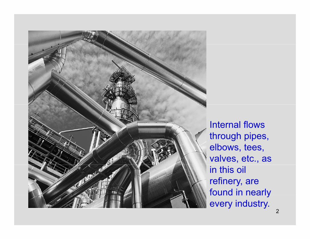
Internal flows through pipesthrough pipes, elbows, tees,valves, etc., as in this oil refinery, are found in nearly

2

found in nearly every industry.

Objectives• Have a deeper understanding of laminar and

turbulent flow in pipes and the analysis of fully developed flow

• Calculate the major and minor losses associated with pipe flow in piping networks and determinewith pipe flow in piping networks and determine the pumping power requirements

• Understand various velocity and flow rateUnderstand various velocity and flow rate measurement techniques and learn theiradvantages and disadvantages

3

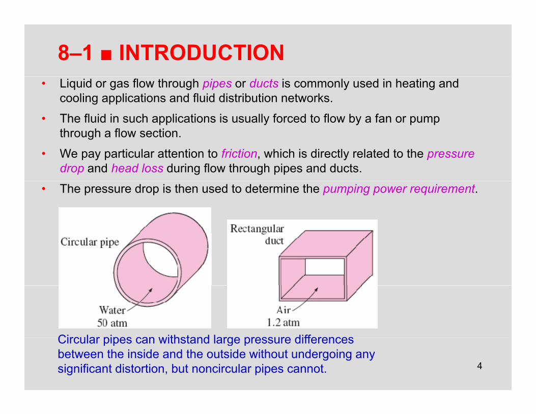
8–1 ■ INTRODUCTION• Liquid or gas flow through pipes or ducts is commonly used in heating and

cooling applications and fluid distribution networks.

• The fluid in such applications is usually forced to flow by a fan or pumpth h fl tithrough a flow section.

• We pay particular attention to friction, which is directly related to the pressuredrop and head loss during flow through pipes and ducts.

• The pressure drop is then used to determine the pumping power requirement.

Circular pipes can withstand large pressure differences

4

Circular pipes can withstand large pressure differences between the inside and the outside without undergoing any significant distortion, but noncircular pipes cannot.

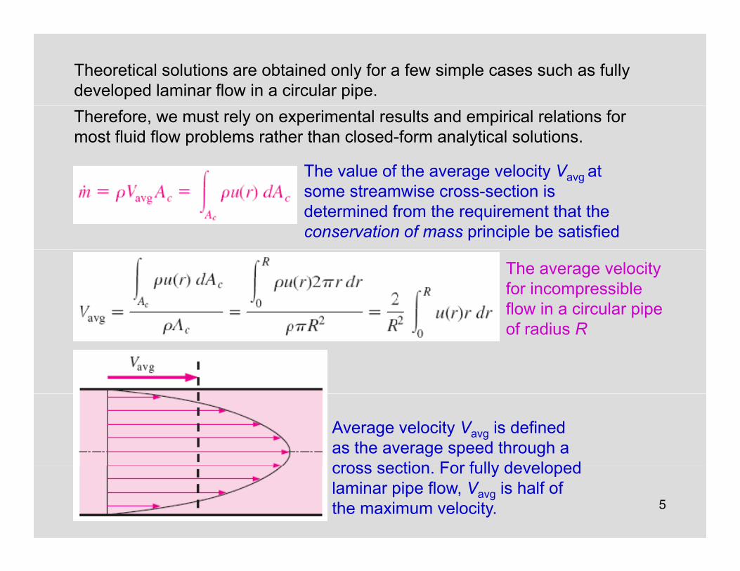
Theoretical solutions are obtained only for a few simple cases such as fully developed laminar flow in a circular pipe. Therefore, we must rely on experimental results and empirical relations for most fluid flow problems rather than closed-form analytical solutions.

The value of the average velocity Vavg at g y avg some streamwise cross-section isdetermined from the requirement that the conservation of mass principle be satisfied

The average velocity for incompressibleflow in a circular pipe of radius R

Average velocity Vavg is defined as the average speed through a cross section For fully developed

5

cross section. For fully developed laminar pipe flow, Vavg is half of the maximum velocity.

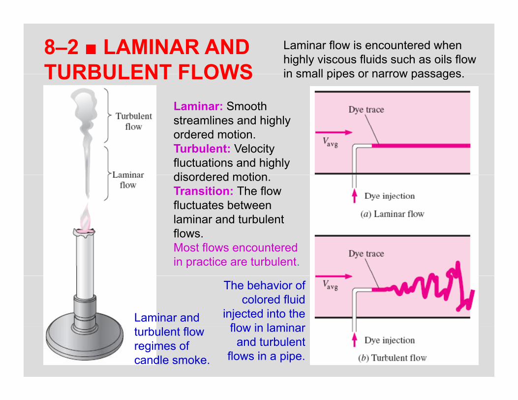
8–2 ■ LAMINAR AND TURBULENT FLOWS

Laminar flow is encountered when highly viscous fluids such as oils flow in small pipes or narrow passagesTURBULENT FLOWS

Laminar: Smooth streamlines and highly

in small pipes or narrow passages.

g yordered motion.Turbulent: Velocity fluctuations and highly disordered motiondisordered motion. Transition: The flow fluctuates between laminar and turbulent flows.Most flows encountered in practice are turbulent.

Laminar and

The behavior of colored fluid

injected into the flow in laminar

6

turbulent flow regimes of candle smoke.

flow in laminar and turbulent

flows in a pipe.

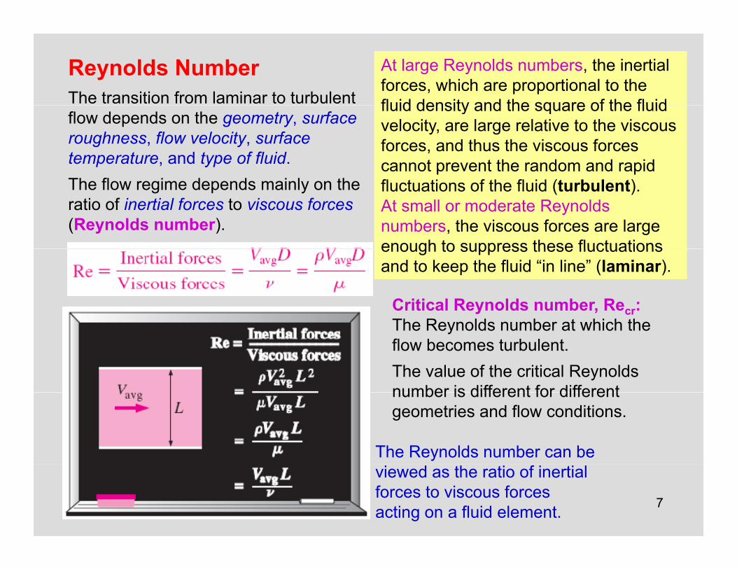
Reynolds NumberThe transition from laminar to turbulent

At large Reynolds numbers, the inertial forces, which are proportional to the fluid density and the square of the fluid

flow depends on the geometry, surfaceroughness, flow velocity, surface temperature, and type of fluid.

fluid density and the square of the fluid velocity, are large relative to the viscous forces, and thus the viscous forces cannot prevent the random and rapid

The flow regime depends mainly on the ratio of inertial forces to viscous forces(Reynolds number).

fluctuations of the fluid (turbulent).At small or moderate Reynolds numbers, the viscous forces are large enough to suppress these fluctuations

Critical Reynolds number, Recr:Th R ld b t hi h th

enough to suppress these fluctuations and to keep the fluid “in line” (laminar).

The Reynolds number at which the flow becomes turbulent. The value of the critical Reynolds number is different for different

The Reynolds number can be

number is different for different geometries and flow conditions.

7

viewed as the ratio of inertial forces to viscous forces acting on a fluid element.

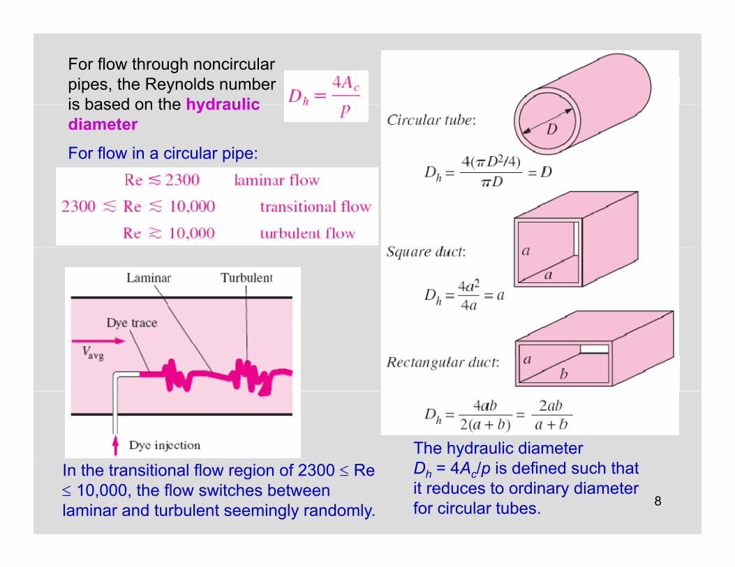
For flow through noncircular pipes, the Reynolds number is based on the hydraulicis based on the hydraulic diameter

For flow in a circular pipe:

The hydraulic diameter D 4A / i d fi d h th t

8

Dh = 4Ac/p is defined such that it reduces to ordinary diameter for circular tubes.

In the transitional flow region of 2300 ≤ Re≤ 10,000, the flow switches between laminar and turbulent seemingly randomly.

8–3 ■ THE ENTRANCE REGIONVelocity boundary layer: The region of the flow in which the effects of the viscous shearing forces caused by fluid viscosity are felt.Boundary layer region: The viscous effects and the velocity changes are significant. Irrotational (core) flow region: The frictional effects are negligible and theIrrotational (core) flow region: The frictional effects are negligible and the velocity remains essentially constant in the radial direction.

9

The development of the velocity boundary layer in a pipe. The developed average velocity profile is parabolic in laminar flow, but somewhat flatter or fuller in turbulent flow.

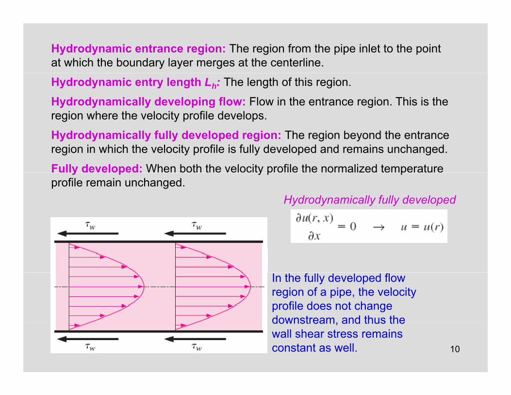
Hydrodynamic entrance region: The region from the pipe inlet to the point at which the boundary layer merges at the centerline.

Hydrodynamic entry length Lh: The length of this region.

Hydrodynamically developing flow: Flow in the entrance region. This is the region where the velocity profile develops.

Hydrodynamically fully developed region: The region beyond the entrance region in which the velocity profile is fully developed and remains unchanged.

Fully developed: When both the velocity profile the normalized temperature y p y p pprofile remain unchanged.

Hydrodynamically fully developed

In the fully developed flow region of a pipe, the velocity profile does not change downstream and thus the

10

downstream, and thus the wall shear stress remains constant as well.

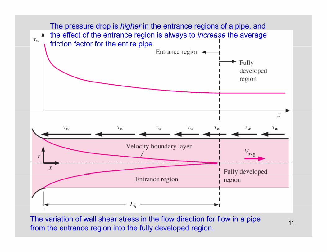
The pressure drop is higher in the entrance regions of a pipe, and the effect of the entrance region is always to increase the averagefriction factor for the entire pipe.p p

11The variation of wall shear stress in the flow direction for flow in a pipefrom the entrance region into the fully developed region.

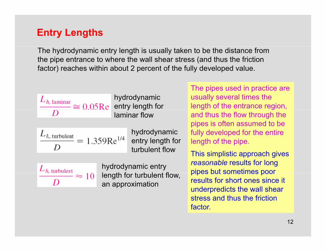
Entry Lengths

The hydrodynamic entry length is usually taken to be the distance from the pipe entrance to where the wall shear stress (and thus the friction factor) reaches within about 2 percent of the fully developed value.

hydrodynamic entry length for

The pipes used in practice are usually several times the length of the entrance region, y g

laminar flow

hydrodynamic entry length for

g gand thus the flow through the pipes is often assumed to be fully developed for the entire length of the pipeentry length for

turbulent flow

hydrodynamic entry l th f t b l t fl

length of the pipe.

This simplistic approach gives reasonable results for long pipes but sometimes poorlength for turbulent flow,

an approximation

pipes but sometimes poor results for short ones since it underpredicts the wall shear stress and thus the friction f t

12

factor.

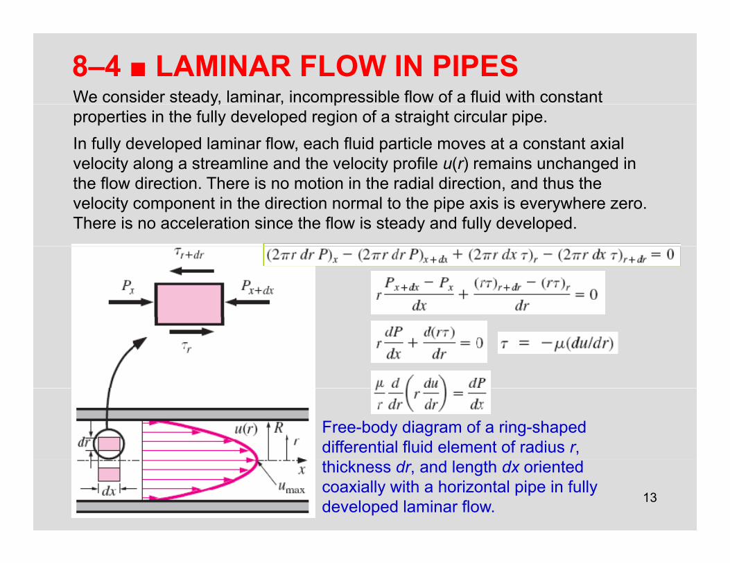
8–4 ■ LAMINAR FLOW IN PIPESWe consider steady, laminar, incompressible flow of a fluid with constanty, , pproperties in the fully developed region of a straight circular pipe.In fully developed laminar flow, each fluid particle moves at a constant axialvelocity along a streamline and the velocity profile u(r) remains unchanged inthe flow direction. There is no motion in the radial direction, and thus thevelocity component in the direction normal to the pipe axis is everywhere zero.There is no acceleration since the flow is steady and fully developed.

Free-body diagram of a ring-shapeddifferential fluid element of radius r,

13

thickness dr, and length dx orientedcoaxially with a horizontal pipe in fully developed laminar flow.

Boundary yconditions

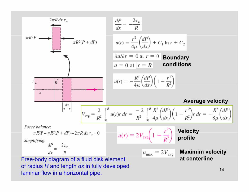
Average velocity

Velocity

Maximim velocity t t li

Velocity profile

14

Free-body diagram of a fluid disk element of radius R and length dx in fully developed laminar flow in a horizontal pipe.

at centerline

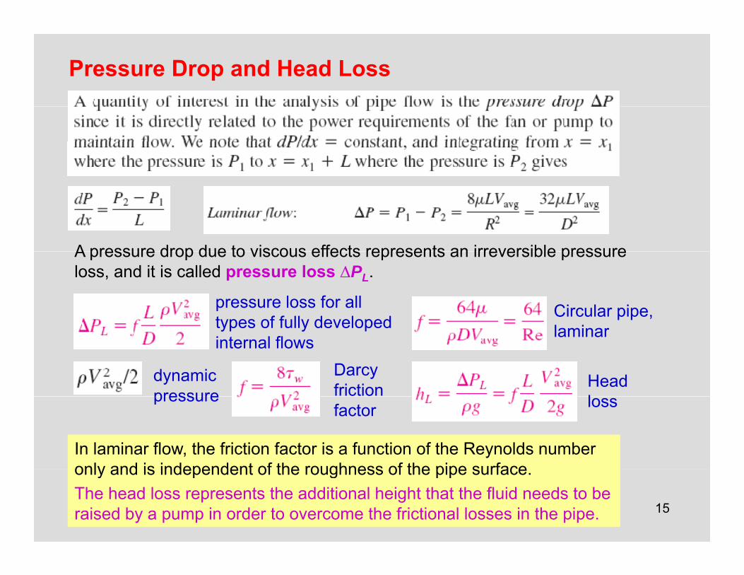
Pressure Drop and Head Loss

A pressure drop due to viscous effects represents an irreversible pressureA pressure drop due to viscous effects represents an irreversible pressure loss, and it is called pressure loss ∆PL.

pressure loss for all types of fully developed

Circular pipe, types of fully developed internal flows

dynamic pressure

Darcy friction

laminar

Head lpressure

factor loss

In laminar flow, the friction factor is a function of the Reynolds number only and is independent of the roughness of the pipe surface

15

only and is independent of the roughness of the pipe surface.The head loss represents the additional height that the fluid needs to beraised by a pump in order to overcome the frictional losses in the pipe.

Horizontal pipe

Poiseuille’s law

For a specified flow rate, the pressure drop and thus the required pumping power is proportional to the length of the pipe and the viscosity of the fluid, but it is inversely proportional to the fourth power of the diameter of the pipe.power of the diameter of the pipe.

The relation for pressure loss (andhead loss) is one of the most generalrelations in fluid mechanics, and it isvalid for laminar or turbulent flows

16

valid for laminar or turbulent flows,circular or noncircular pipes, andpipes with smooth or rough surfaces.

The pumping power requirement for a laminar flow piping system can be reduced by a factor of 16 by doubling the pipe diameter.

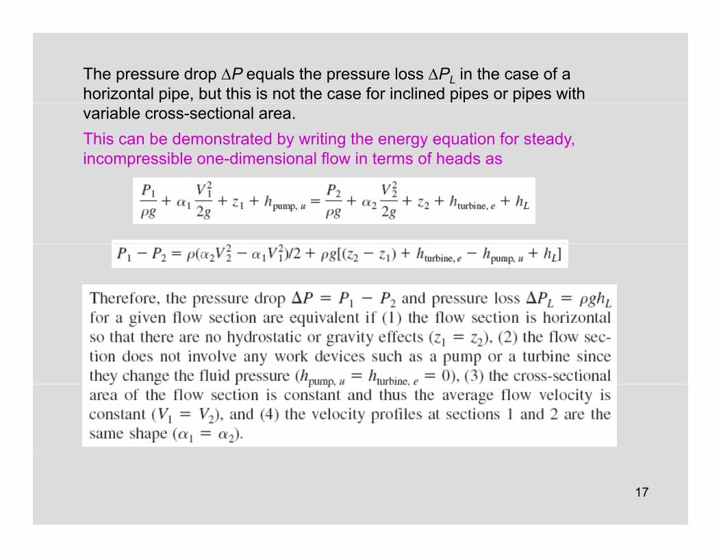
The pressure drop ∆P equals the pressure loss ∆PL in the case of a horizontal pipe, but this is not the case for inclined pipes or pipes with variable cross-sectional area. This can be demonstrated by writing the energy equation for steady, incompressible one-dimensional flow in terms of heads as

17

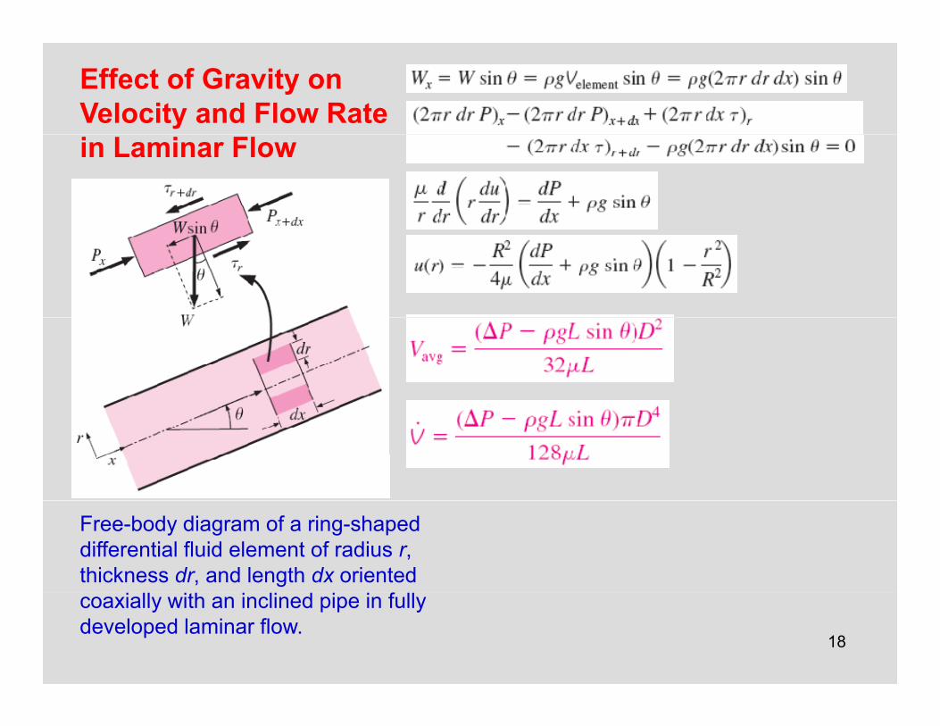
Effect of Gravity on Velocity and Flow Rate in Laminar Flow

Free-body diagram of a ring-shapeddifferential fluid element of radius r,thickness dr, and length dx oriented

18

coaxially with an inclined pipe in fullydeveloped laminar flow.

19

Laminar Flow in Noncircular Pipes

The friction factor f relations are given in Table 8–1 for fully d l d l i fl i

Noncircular Pipes

developed laminar flow in pipes of various cross sections. The Reynolds number for flow in these pipes u be o o ese p pesis based on the hydraulic diameter Dh = 4Ac /p, where Acis the cross-sectional area of the pipe and p is its wettedthe pipe and p is its wetted perimeter

20

21

22

23

24

25

26

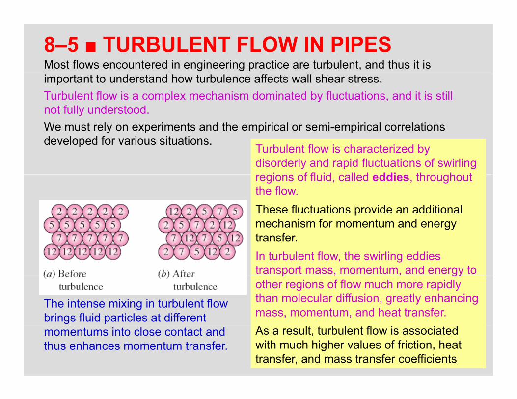
8–5 ■ TURBULENT FLOW IN PIPESMost flows encountered in engineering practice are turbulent, and thus it isimportant to understand how turbulence affects wall shear stress. Turbulent flow is a complex mechanism dominated by fluctuations, and it is still not fully understood.W t l i t d th i i l i i i l l tiWe must rely on experiments and the empirical or semi-empirical correlations developed for various situations.

Turbulent flow is characterized bydisorderly and rapid fluctuations of swirling

i f fl id ll d ddi th h tregions of fluid, called eddies, throughout the flow.These fluctuations provide an additional mechanism for momentum and energymechanism for momentum and energy transfer.In turbulent flow, the swirling eddiestransport mass, momentum, and energy to

The intense mixing in turbulent flowbrings fluid particles at different

p , , gyother regions of flow much more rapidlythan molecular diffusion, greatly enhancing mass, momentum, and heat transfer.

27

momentums into close contact andthus enhances momentum transfer.

As a result, turbulent flow is associated with much higher values of friction, heat transfer, and mass transfer coefficients

The laminar component: accounts for the friction between layers in the flow directionThe turbulent component: accounts for theThe turbulent component: accounts for the friction between the fluctuating fluid particles and the fluid body (related to the fluctuation components of velocity).

Fluctuations of the velocity component u with time at a specified location in turbulent flow.

28

The velocity profile and the variation of shear stress with radial distance

for turbulent flow in a pipe.

Turbulent Shear Stress

turbulent shear stress

Turbulent shearTurbulent shear stress

eddy viscosity or turbulent viscosity: t f t t t baccounts for momentum transport by

turbulent eddies.

Total shear t

Fluid particle moving upward through a

stress

kinematic eddy viscosity or kinematic turbulent viscosity (also called the

29

differential area dA as a result of the velocity fluctuation v.

turbulent viscosity (also called the eddy diffusivity of momentum).

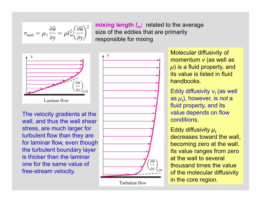
mixing length lm: related to the average size of the eddies that are primarily

ibl f i iresponsible for mixing

Molecular diffusivity of momentum v (as well as (µ) is a fluid property, and its value is listed in fluid handbooks.

The velocity gradients at the

Eddy diffusivity vt (as well as µt), however, is not a fluid property, and its value depends on flowThe velocity gradients at the

wall, and thus the wall shear stress, are much larger for turbulent flow than they are

value depends on flow conditions.

Eddy diffusivity µtdecreases toward the wall,

for laminar flow, even though the turbulent boundary layer is thicker than the laminar one for the same value of

,becoming zero at the wall. Its value ranges from zero at the wall to several thousand times the value

30

one for the same value of free-stream velocity.

thousand times the value of the molecular diffusivity in the core region.

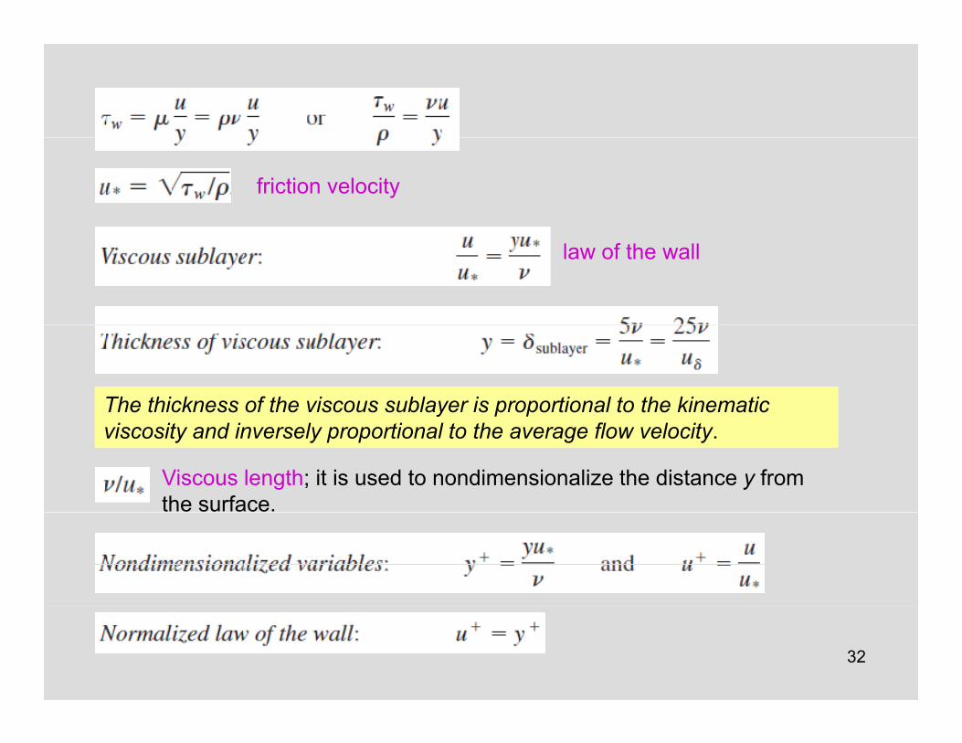
Turbulent Velocity Profile The very thin layer next to the wall where viscous effects are dominant is the viscous(or laminar or linear or wall) sublayer(or laminar or linear or wall) sublayer.

The velocity profile in this layer is very nearly linear, and the flow is streamlined.

N t t th i bl i th b ffNext to the viscous sublayer is the buffer layer, in which turbulent effects are becoming significant, but the flow is still dominated by viscous effects.

Above the buffer layer is the overlap (or transition) layer, also called the inertial sublayer, in which the turbulent effects are much more significant, but still not dominant.

Above that is the outer (or turbulent) layer in the remaining part of the flow in which t b l t ff t d i t l l

The velocity profile in fully developed pipe flow is parabolic in laminar

turbulent effects dominate over molecular diffusion (viscous) effects.

31

The velocity profile in fully developed pipe flow is parabolic in laminar flow, but much fuller in turbulent flow. Note that u(r) in the turbulent case is the time-averaged velocity component in the axial direction (the overbar on u has been dropped for simplicity).

friction velocity

law of the wall

The thickness of the viscous sublayer is proportional to the kinematic viscosity and inversely proportional to the average flow velocity.

Viscous length; it is used to nondimensionalize the distance y from the surface.

32

Comparison of the law of the wall and the logarithmic-law velocity profiles with experimental data

33

for fully developed turbulent flow in a pipe.

Velocity defect lawdefect law

The deviation of velocity from the centerline value umax - u is called the velocity defect.y

The value n = 7 generally approximates many flows in practice, giving rise to the term one-seventh

l l it filpower-law velocity profile.

Power-law velocity profiles for fully developed turbulent flow in a pipe for different exponents and its

34

exponents, and its comparison with the laminar velocity profile.

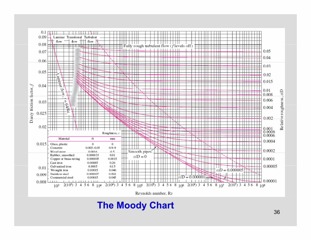
The Moody Chart and

C l b k ti (f th d h i )theColebrook Equation

The friction factor in fully developed turbulent pipe flow depends on the Reynolds number and the relative roughness ε /D.

Colebrook equation (for smooth and rough pipes)

q

Explicit Haaland equation

The friction factor is minimum for a

35

smooth pipe and increases with roughness.

36The Moody Chart

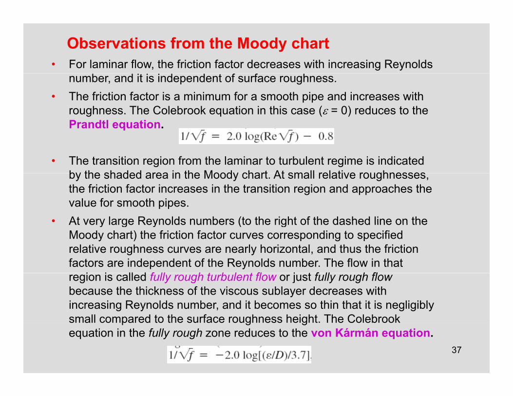
• For laminar flow, the friction factor decreases with increasing Reynolds

Observations from the Moody chart

number, and it is independent of surface roughness.• The friction factor is a minimum for a smooth pipe and increases with

roughness. The Colebrook equation in this case (ε = 0) reduces to the Prandtl equationPrandtl equation.

• The transition region from the laminar to turbulent regime is indicated by the shaded area in the Moody chart At small relative roughnessesby the shaded area in the Moody chart. At small relative roughnesses, the friction factor increases in the transition region and approaches the value for smooth pipes.

• At very large Reynolds numbers (to the right of the dashed line on theAt very large Reynolds numbers (to the right of the dashed line on the Moody chart) the friction factor curves corresponding to specified relative roughness curves are nearly horizontal, and thus the friction factors are independent of the Reynolds number. The flow in that

i i ll d f ll h t b l t fl j t f ll h flregion is called fully rough turbulent flow or just fully rough flow because the thickness of the viscous sublayer decreases with increasing Reynolds number, and it becomes so thin that it is negligibly small compared to the surface roughness height. The Colebrook

37

p g gequation in the fully rough zone reduces to the von Kármán equation.

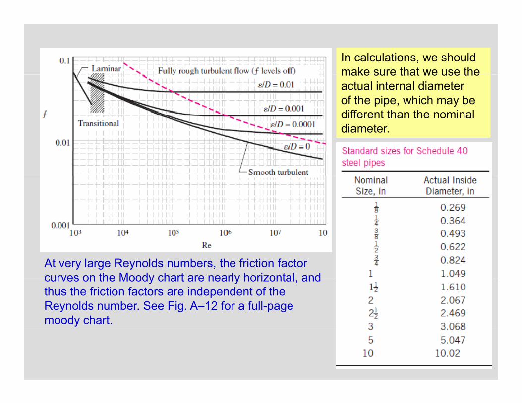
In calculations, we should make sure that we use themake sure that we use the actual internal diameterof the pipe, which may be different than the nominal di tdiameter.

At very large Reynolds numbers, the friction factor curves on the Moody chart are nearly horizontal andcurves on the Moody chart are nearly horizontal, and thus the friction factors are independent of the Reynolds number. See Fig. A–12 for a full-page moody chart.

38

Types of Fluid Flow Problems1 Determining the pressure drop (or head1. Determining the pressure drop (or head

loss) when the pipe length and diameter are given for a specified flow rate (or velocity)

2. Determining the flow rate when the pipe length and diameter are given for a specified pressure drop (or head loss)

The three types of problems3. Determining the pipe diameter when the

pipe length and flow rate are given for a specified pressure drop (or head loss)

e ee ypes o p ob e sencountered in pipe flow.

To avoid tedious iterations in head loss, flow rate, and diameter calculationsdiameter calculations,these explicit relations that are accurate to within 2 percent of the

39

Moody chart may be used.

40

41

42

43

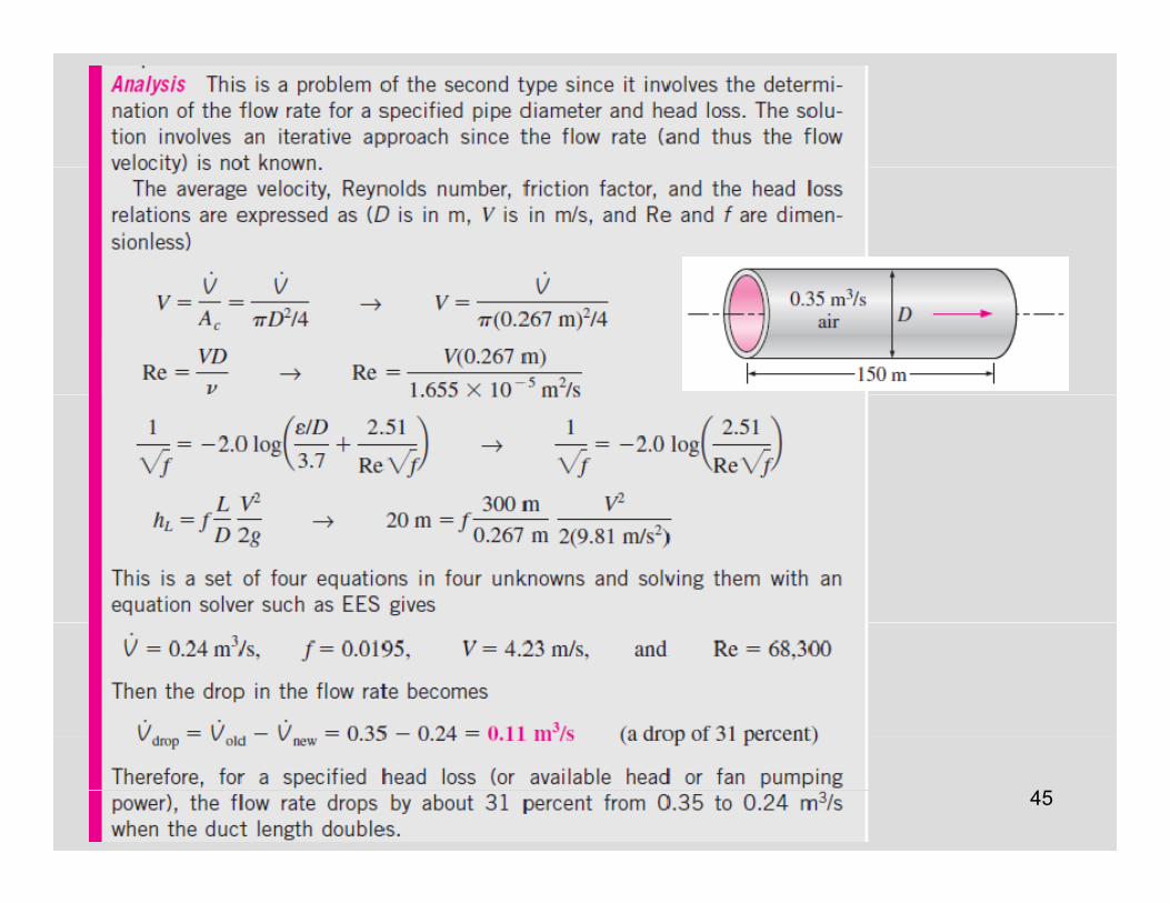
44

45

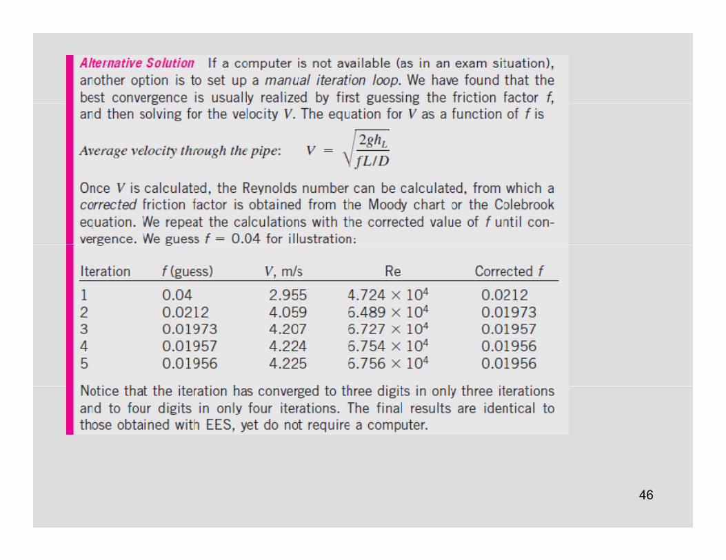
46

47

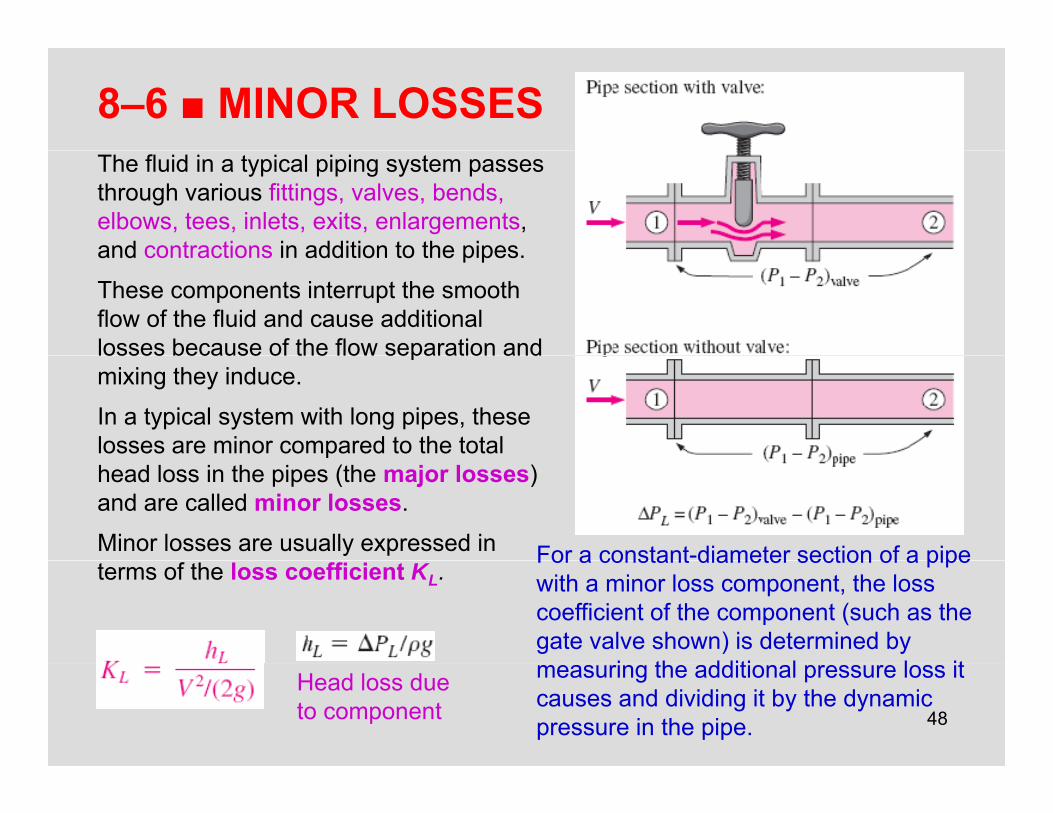
8–6 ■ MINOR LOSSESThe fluid in a typical piping system passes through various fittings, valves, bends, elbows, tees, inlets, exits, enlargements, and contractions in addition to the pipesand contractions in addition to the pipes.

These components interrupt the smooth flow of the fluid and cause additional losses because of the flow separation andlosses because of the flow separation and mixing they induce.

In a typical system with long pipes, these losses are minor compared to the total head loss in the pipes (the major losses) and are called minor losses.

Minor losses are usually expressed in For a constant-diameter section of a pipeterms of the loss coefficient KL.

For a constant diameter section of a pipe with a minor loss component, the loss coefficient of the component (such as the gate valve shown) is determined by

i th dditi l l it

48

measuring the additional pressure loss it causes and dividing it by the dynamicpressure in the pipe.

Head loss due to component

When the inlet diameter equals outlet diameter, the loss coefficient of acomponent can also be determined by measuring the pressure loss across thecomponent and dividing it by the dynamic pressure:pressure:

KL = ∆PL /(ρV2/2).When the loss coefficient for a component i il bl th h d l f th tis available, the head loss for thatcomponent is

Minor lloss

Minor losses are also expressed in terms of the equivalent length Lequiv.

The head loss caused by a component (such as the angle p ( gvalve shown) is equivalent to the head loss caused by a section of the pipe whose length is theequivalent length

49

equivalent length.

Total head loss (general)

Total head loss (D = constant)

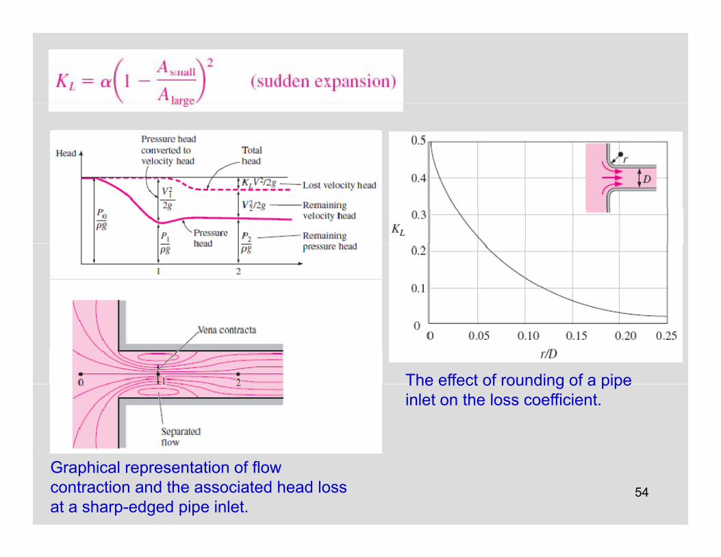
The head loss at the inlet of a pipe is almost negligible for well-

rounded inlets (KL = 0 03 for r/D >

50

rounded inlets (KL 0.03 for r/D >0.2) but increases to about 0.50 for

sharp-edged inlets.

51

52

53

The effect of rounding of a pipeThe effect of rounding of a pipe inlet on the loss coefficient.

54

Graphical representation of flow contraction and the associated head loss at a sharp-edged pipe inlet.

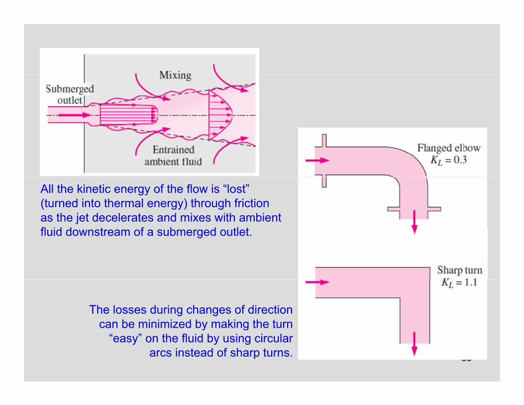
All the kinetic energy of the flow is “lost” (turned into thermal energy) through friction as the jet decelerates and mixes with ambient fl id d t f b d tl tfluid downstream of a submerged outlet.

The losses during changes of directioncan be minimized by making the turn

55

y g“easy” on the fluid by using circular

arcs instead of sharp turns.

(a) The large head loss in a partially closed valve is duepartially closed valve is due to irreversible deceleration, flow separation, and mixing of high-velocity fluid comingg y gfrom the narrow valve passage.(b) The head loss through a

56

fully-open ball valve, on theother hand, is quite small.

57

58

8–7 ■ PIPING NETWORKS AND PUMP SELECTION

For pipes in series, the flow rate is the same

A piping network in an

o p pes se es, e o a e s e sa ein each pipe, and the total head loss is the sum of the head losses in individual pipes.

industrial facility.

For pipes in parallel, the head loss is the same in

each pipe and the total flow

59

each pipe, and the total flow rate is the sum of the flow

rates in individual pipes.

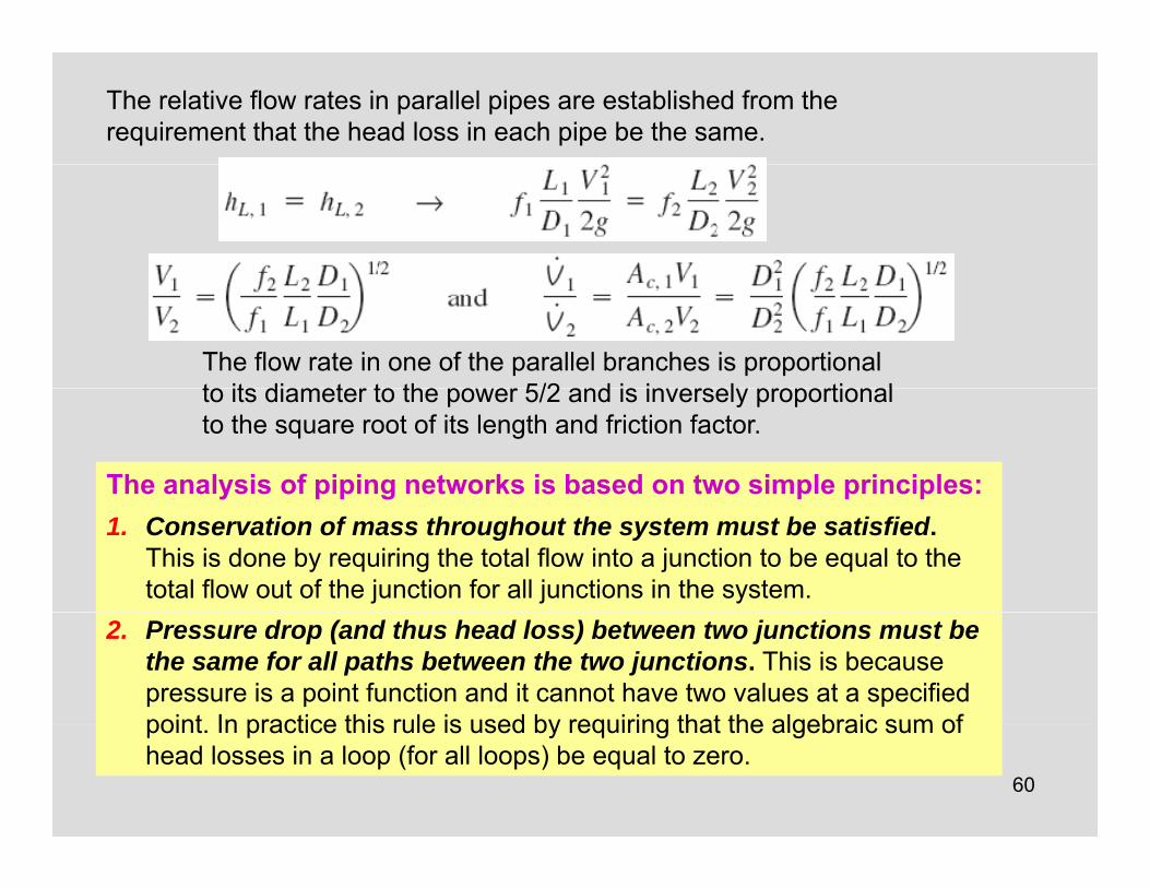
The relative flow rates in parallel pipes are established from therequirement that the head loss in each pipe be the same.

The flow rate in one of the parallel branches is proportionalto its diameter to the po er 5/2 and is in ersel proportional

The analysis of piping networks is based on two simple principles:

to its diameter to the power 5/2 and is inversely proportional to the square root of its length and friction factor.

1. Conservation of mass throughout the system must be satisfied.This is done by requiring the total flow into a junction to be equal to the total flow out of the junction for all junctions in the system.

2. Pressure drop (and thus head loss) between two junctions must be the same for all paths between the two junctions. This is because pressure is a point function and it cannot have two values at a specified point In practice this rule is used by requiring that the algebraic sum of

60

point. In practice this rule is used by requiring that the algebraic sum of head losses in a loop (for all loops) be equal to zero.

Piping Systems with Pumps and Turbines

the steady-flowenergy equation

When a pump moves a fluid from one reservoir

61

to another, the useful pump head requirement is equal to the elevation difference between the two reservoirs plus the head loss.

The efficiency of the pump–motorcombination is the product of thepump and the motor efficiencies.

Ch t i ti f t if l th

62

Characteristic pump curves for centrifugal pumps, the system curve for a piping system, and the operating point.

63

64

65

66

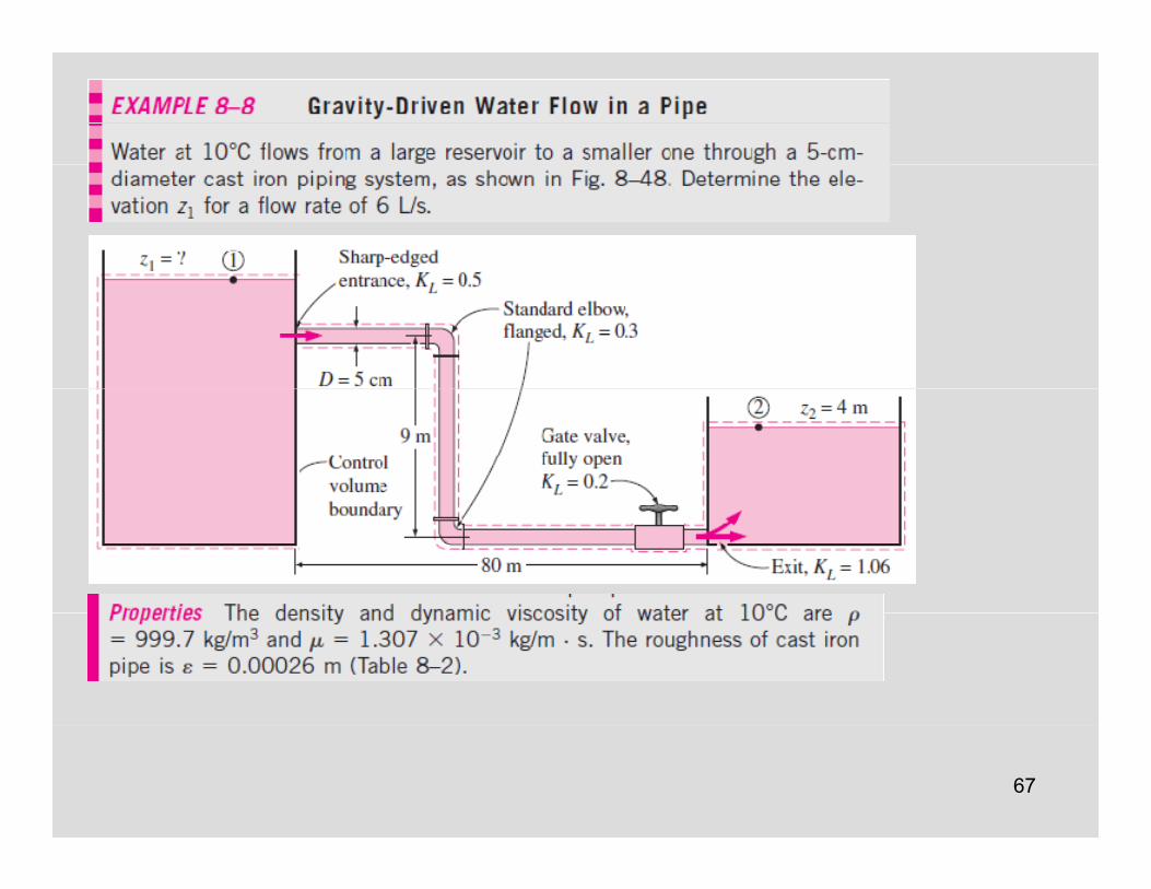
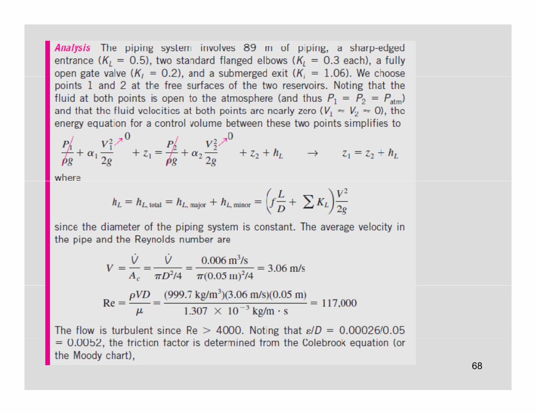
67

68

69

70

71

72

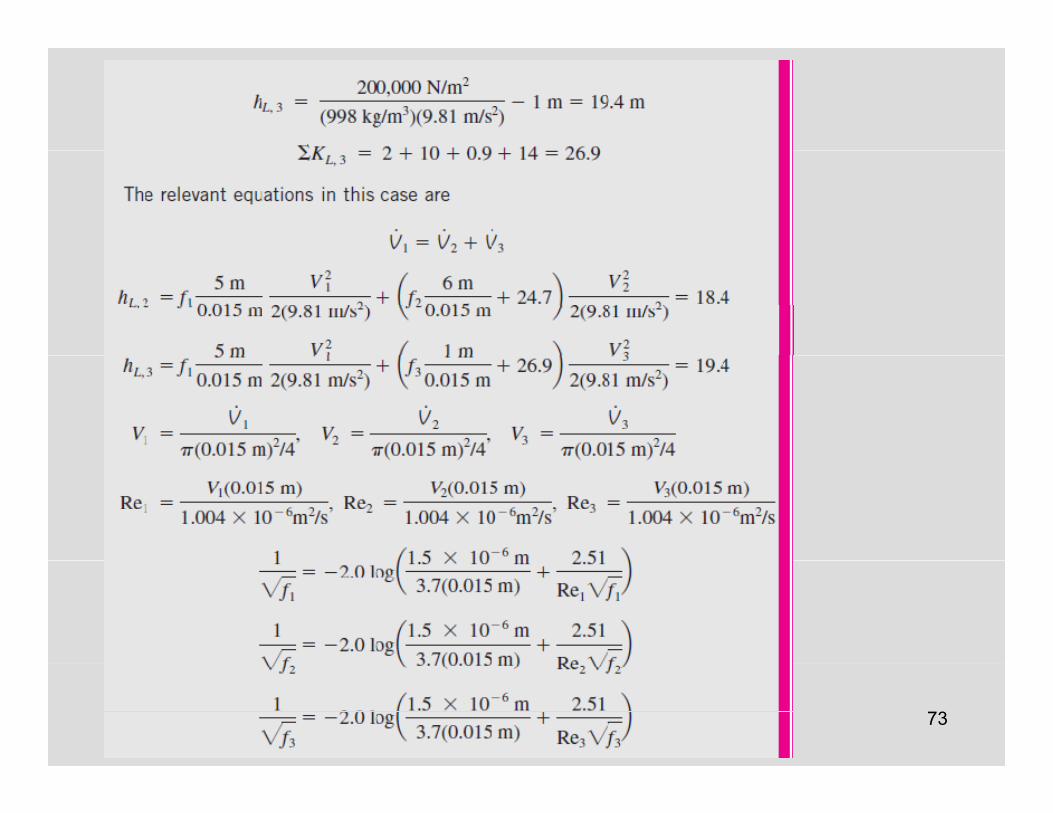
73

74

Flow rate of cold water through a shower may be affected significantly by the flushing of a nearb toilet

75

nearby toilet.

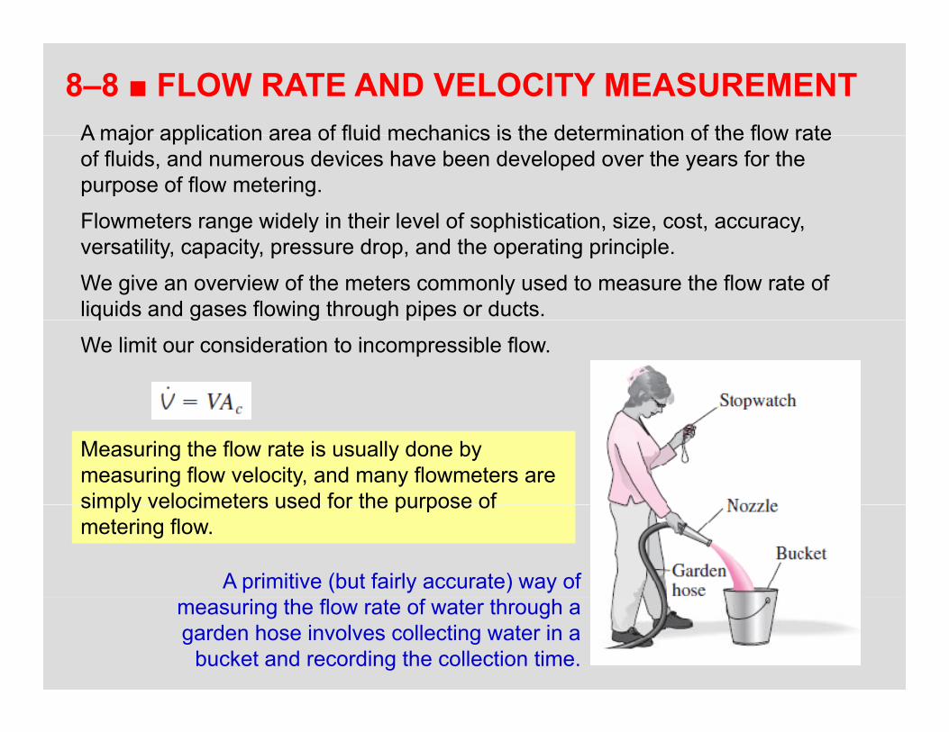
8–8 ■ FLOW RATE AND VELOCITY MEASUREMENTA major application area of fluid mechanics is the determination of the flow rateA major application area of fluid mechanics is the determination of the flow rate of fluids, and numerous devices have been developed over the years for the purpose of flow metering.

Flowmeters range widely in their level of sophistication, size, cost, accuracy,Flowmeters range widely in their level of sophistication, size, cost, accuracy, versatility, capacity, pressure drop, and the operating principle.

We give an overview of the meters commonly used to measure the flow rate of liquids and gases flowing through pipes or ducts. q g g g p p

We limit our consideration to incompressible flow.

Measuring the flow rate is usually done by measuring flow velocity, and many flowmeters aresimply velocimeters used for the purpose of

A primitive (but fairly accurate) way of

simply velocimeters used for the purpose of metering flow.

76

measuring the flow rate of water through a garden hose involves collecting water in a

bucket and recording the collection time.

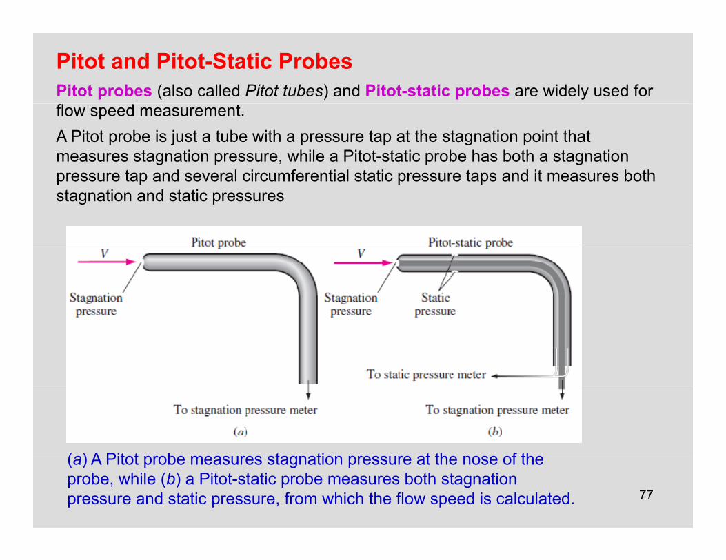
Pitot and Pitot-Static ProbesPitot probes (also called Pitot tubes) and Pitot-static probes are widely used for flow speed measurement.A Pitot probe is just a tube with a pressure tap at the stagnation point that measures stagnation pressure, while a Pitot-static probe has both a stagnation pressure tap and several circumferential static pressure taps and it measures bothpressure tap and several circumferential static pressure taps and it measures both stagnation and static pressures

(a) A Pitot probe measures stagnation pressure at the nose of the

77

(a) A Pitot probe measures stagnation pressure at the nose of the probe, while (b) a Pitot-static probe measures both stagnation pressure and static pressure, from which the flow speed is calculated.

Measuring flow velocity with a Pitotstatic probe. (A manometer may be used in place of the

Close-up of a Pitot-static probe, showing the stagnation pressure hole and two of th fi t ti i f ti l

78

may be used in place of the differential pressure transducer.)

the five static circumferential pressure holes.

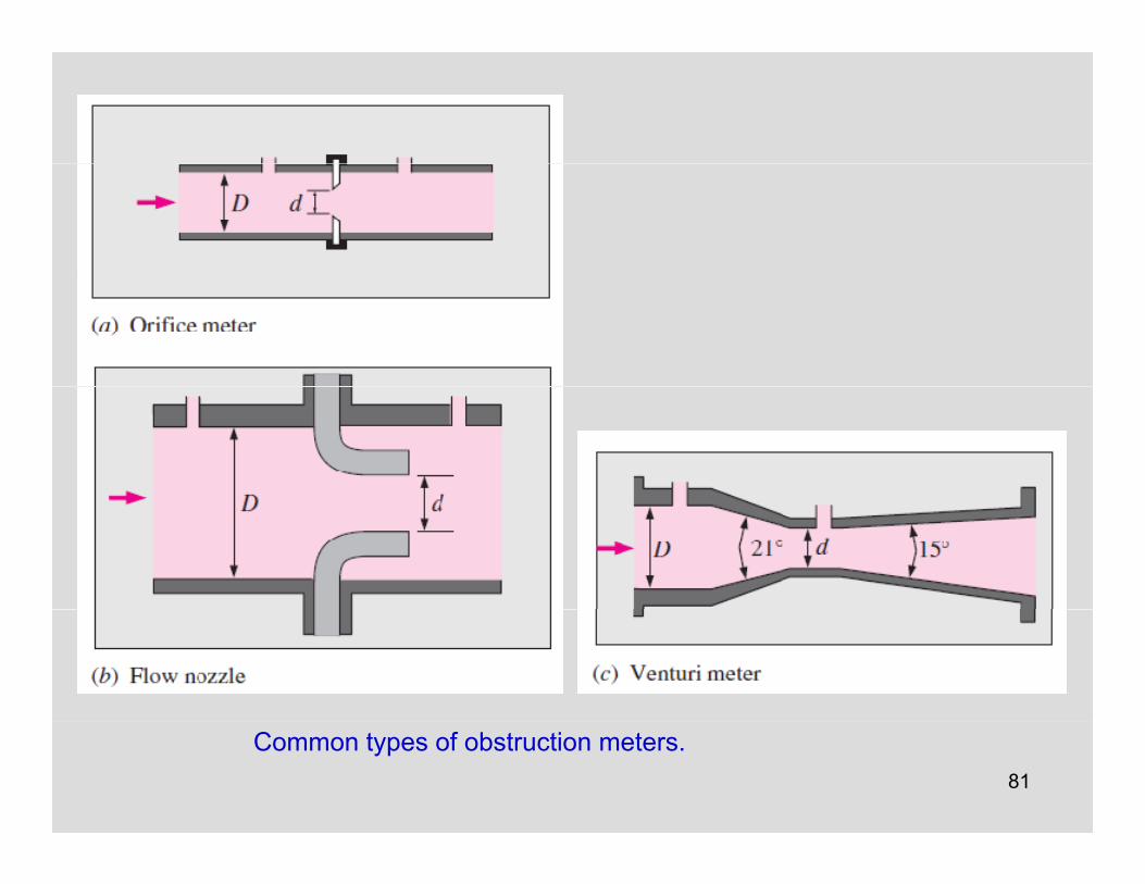
Obstruction Flowmeters: Orifice Venturi andOrifice, Venturi, and Nozzle Meters

Flowmeters based on this principleFlowmeters based on this principle are called obstruction flowmetersand are widely used to measure flow rates of gases and liquids.

Flow through a constriction in a pipe.

79

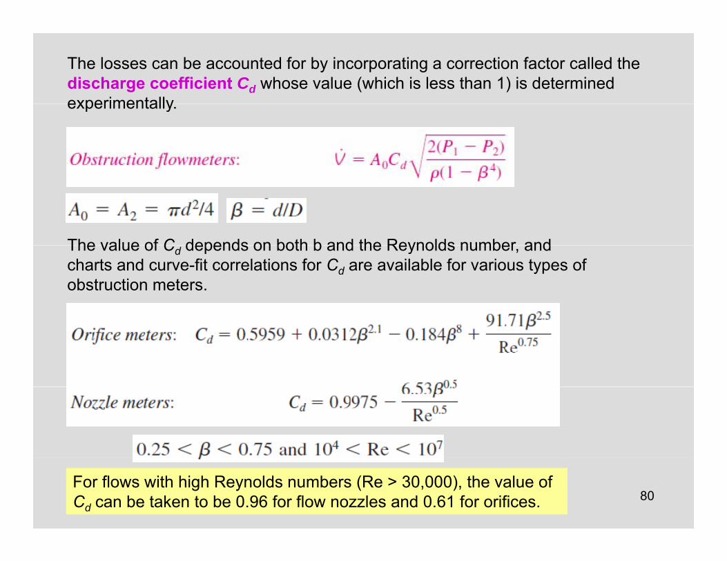
The losses can be accounted for by incorporating a correction factor called the discharge coefficient Cd whose value (which is less than 1) is determined experimentallyexperimentally.

The value of C depends on both b and the Reynolds number andThe value of Cd depends on both b and the Reynolds number, and charts and curve-fit correlations for Cd are available for various types of obstruction meters.

80For flows with high Reynolds numbers (Re > 30,000), the value of Cd can be taken to be 0.96 for flow nozzles and 0.61 for orifices.

81

Common types of obstruction meters.

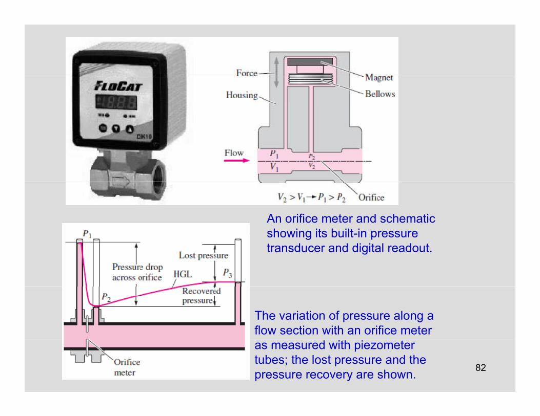
An orifice meter and schematic showing its built-in pressureshowing its built-in pressure transducer and digital readout.

The variation of pressure along a flow section with an orifice meter

82

as measured with piezometer tubes; the lost pressure and the pressure recovery are shown.

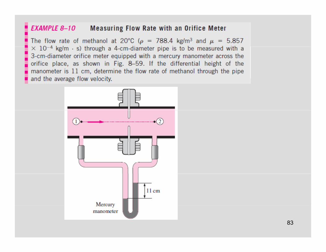
83

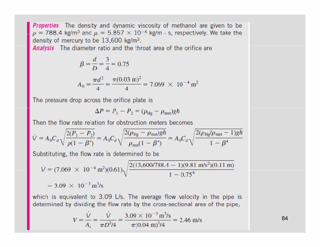
84

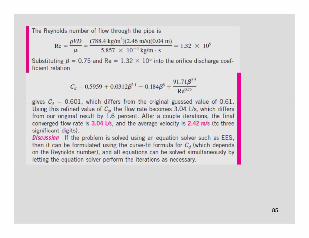
85

The total amount of mass or volume of a fluid that th h ti f i

Positive Displacement Flowmeters

passes through a cross section of a pipe over a certain period of time is measured by positive displacement flowmeters.There are numerous types of displacementThere are numerous types of displacement meters, and they are based on continuous filling and discharging of the measuring chamber. They operate by trapping a certain amount of incoming fluid, displacing it to the discharge side of the meter, and counting the number of such discharge–recharge cycles to determine the total amount of fluid displaced.amount of fluid displaced.

A positive displacement flowmeter with

86A nutating disk flowmeter.

double helical three-lobe impeller design.

Turbine Flowmeters

(a) An in-line turbine flowmeter to measure liquid flow, with flow from left to right, (b) a cutaway view of the turbine blades inside the flowmeter, and (c) a handheld turbine flowmeter to measure wind speed, measuring no flow at the time the photo was taken so that the turbine blades are visible. The flowmeter in (c) also measures the air termperature for convenience.

87

Paddlewheel Flowmeters

Paddlewheel flowmeters are low-cost alternatives to turbine flowmeters for flows where very high accuracy is not requiredrequired.The paddlewheel (the rotor and the blades) is perpendicular to the flow rather than parallel as was the case pwith turbine flowmeters.

Paddlewheel flowmeter to measure liquid flow, with

flow from left to right, and a

88

g ,schematic diagram of

its operation.

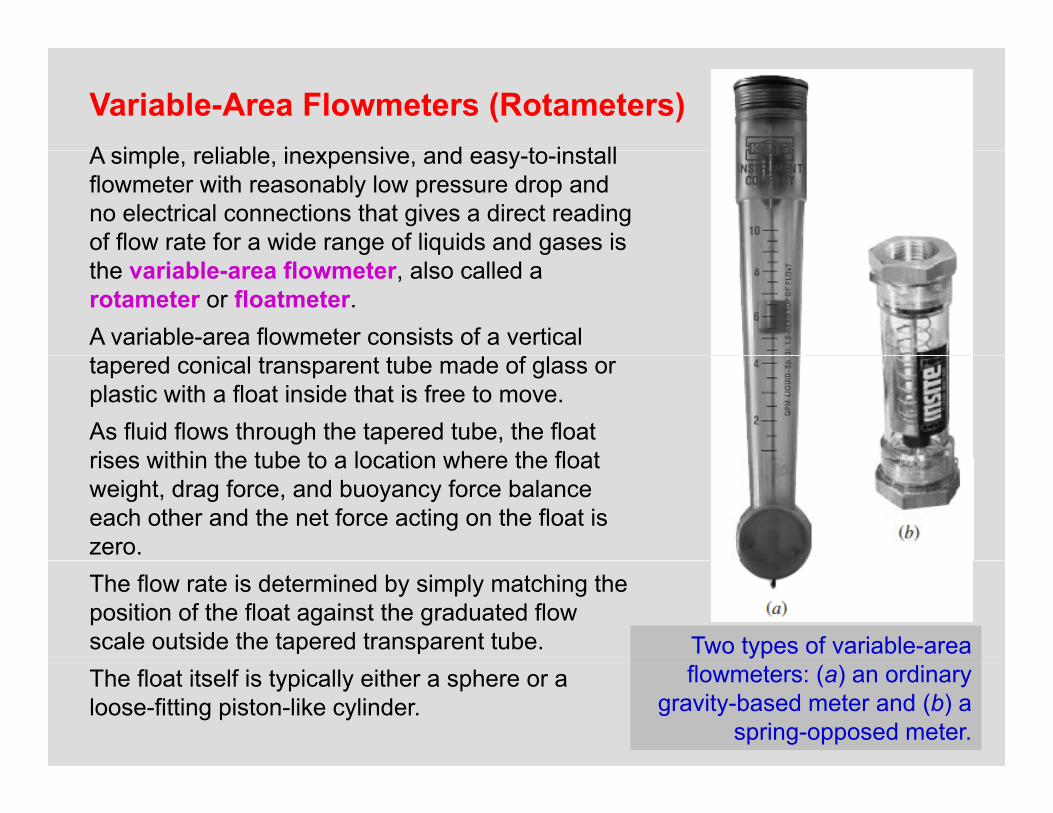
Variable-Area Flowmeters (Rotameters)A i l li bl i i d t i t llA simple, reliable, inexpensive, and easy-to-install flowmeter with reasonably low pressure drop and no electrical connections that gives a direct reading of flow rate for a wide range of liquids and gases is g q gthe variable-area flowmeter, also called a rotameter or floatmeter. A variable-area flowmeter consists of a vertical tapered conical transparent tube made of glass or plastic with a float inside that is free to move.As fluid flows through the tapered tube, the float rises within the tube to a location where the floatrises within the tube to a location where the float weight, drag force, and buoyancy force balance each other and the net force acting on the float is zero. The flow rate is determined by simply matching the position of the float against the graduated flow scale outside the tapered transparent tube. Two types of variable-area

89

The float itself is typically either a sphere or a loose-fitting piston-like cylinder.

flowmeters: (a) an ordinary gravity-based meter and (b) a

spring-opposed meter.

Ultrasonic FlowmetersUltrasonic flowmeters operate using sound waves in the ultrasonic rangeUltrasonic flowmeters operate using sound waves in the ultrasonic range ( beyond human hearing ability, typically at a frequency of 1 MHz).Ultrasonic (or acoustic) flowmeters operate by generating sound waves with a transducer and measuring the propagation of those waves through a g p p g gflowing fluid. There are two basic kinds of ultrasonic flowmeters: transit time and Doppler-effect (or frequency shift) flowmeters.

L is the distance between the transducers and K is a constant

90

The operation of a transit time ultrasonic flowmeter equipped with two transducers.

Doppler-Effect UltrasonicUltrasonic Flowmeters

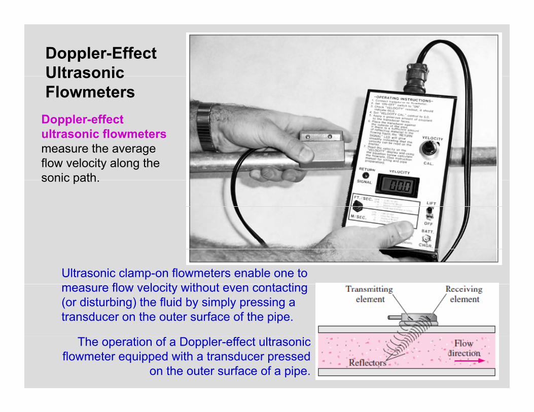
Doppler-effect ultrasonic flowmetersmeasure the average flow velocity along the sonic pathsonic path.

Ultrasonic clamp-on flowmeters enable one to fl l it ith t t timeasure flow velocity without even contacting

(or disturbing) the fluid by simply pressing a transducer on the outer surface of the pipe.

91

The operation of a Doppler-effect ultrasonic flowmeter equipped with a transducer pressed

on the outer surface of a pipe.

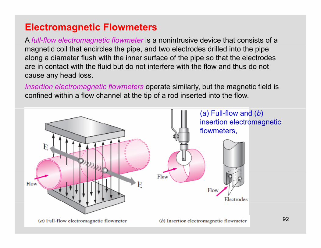
Electromagnetic FlowmetersA full-flow electromagnetic flowmeter is a nonintrusive device that consists of a magnetic coil that encircles the pipe, and two electrodes drilled into the pipe along a diameter flush with the inner surface of the pipe so that the electrodes are in contact with the fluid but do not interfere with the flow and thus do not cause any head loss.cause any head loss.Insertion electromagnetic flowmeters operate similarly, but the magnetic field is confined within a flow channel at the tip of a rod inserted into the flow.

(a) Full-flow and (b) insertion electromagnetic flowmeters,

92

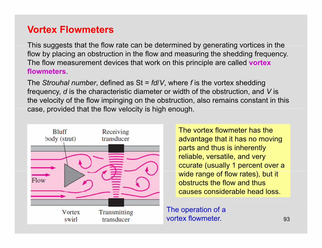
Vortex FlowmetersThis suggests that the flow rate can be determined by generating vortices in theThis suggests that the flow rate can be determined by generating vortices in the flow by placing an obstruction in the flow and measuring the shedding frequency. The flow measurement devices that work on this principle are called vortex flowmeters. The Strouhal number, defined as St = fd/V, where f is the vortex shedding frequency, d is the characteristic diameter or width of the obstruction, and V is the velocity of the flow impinging on the obstruction, also remains constant in this case provided that the flow velocity is high enoughcase, provided that the flow velocity is high enough.

The vortex flowmeter has the advantage that it has no movingadvantage that it has no moving parts and thus is inherently reliable, versatile, and very ccurate (usually 1 percent over a wide range of flow rates), but it obstructs the flow and thus causes considerable head loss.

93The operation of a vortex flowmeter.

Thermal (Hot-Wire and Hot-Film) AnemometersThermal anemometers involve an electrically heated sensor and utilize a thermalThermal anemometers involve an electrically heated sensor and utilize a thermal effect to measure flow velocity.Thermal anemometers have extremely small sensors, and thus they can be used to measure the instantaneous velocity at any point in the flow without appreciablyto measure the instantaneous velocity at any point in the flow without appreciably disturbing the flow.They can measure velocities in liquids and gases accurately over a wide range—from a few centimeters to over a hundred meters per second.

A thermal anemometer is called a hot-wire anemometer if the sensing element is a wire and a hot-filmelement is a wire, and a hot film anemometer if the sensor is a thin metallic film (less than 0.1 µm thick) mounted usually on a relatively thick

i t h i di t f

The electrically heated sensor

ceramic support having a diameter of about 50 µm.

94

The electrically heated sensor and its support, components of a hot-wire probe.

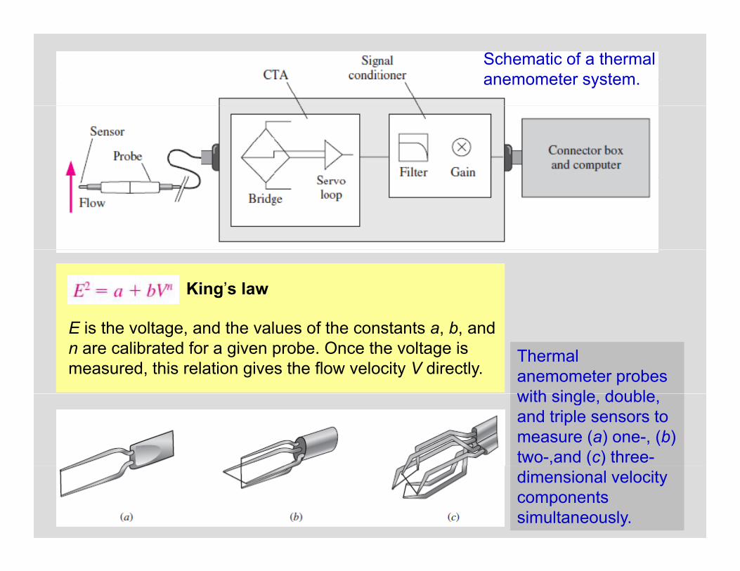
Schematic of a thermal anemometer system.

King’s law

E i h l d h l f h b dE is the voltage, and the values of the constants a, b, and n are calibrated for a given probe. Once the voltage is measured, this relation gives the flow velocity V directly.

Thermal anemometer probes with single doublewith single, double, and triple sensors to measure (a) one-, (b) two-,and (c) three-

95

( )dimensional velocity components simultaneously.

Laser Doppler VelocimetryLaser Doppler velocimetry (LDV) also called laser velocimetry (LV) or laserLaser Doppler velocimetry (LDV), also called laser velocimetry (LV) or laser Doppler anemometry (LDA), is an optical technique to measure flow velocity at any desired point without disturbing the flow.Unlike thermal anemometry, LDV involves no probes or wires inserted into the y, pflow, and thus it is a nonintrusive method. Like thermal anemometry, it can accurately measure velocity at a very small volume, and thus it can also be used to study the details of flow at a locality, including turbulent fluctuations, and it can be traversed through the entire flow field without intrusion.

96A dual-beam LDV system in forward scatter mode.

LDV equation

λ is the wavelength of the laser beam and α is the angle between the two laser beamsThis fundamental relation shows the flow velocity to be proportional to the frequency.

the angle between the two laser beams

Fringes that form as a result of the interference at the intersection of two laserintersection of two laser beams of an LDV system (lines represent peaks of waves). The top diagram is

l i f t

A time-averaged velocity profile in

97

a close-up view of two fringes.

turbulent pipe flow obtained by an

LDV system.

Particle Image VelocimetryParticle image velocimetry (PIV) is a double-pulsed laser technique used toParticle image velocimetry (PIV) is a double-pulsed laser technique used to measure the instantaneous velocity distribution in a plane of flow by photographically determining the displacement of particles in the plane during a very short time interval. Unlike methods like hot-wire anemometry and LDV that measure velocity at a point, PIV provides velocity values simultaneously throughout an entire cross section, and thus it is a whole-field technique. PIV combines the accuracy of LDV with the capability of flow visualization and provides instantaneous flow field mapping.The entire instantaneous velocity profile at a cross section of pipe can beobtained with a single PIV measurementobtained with a single PIV measurement.A PIV system can be viewed as a camera that can take a snapshot of velocity distribution at any desired plane in a flow. Ordinary flow visualization gives a qualitative picture of the details of flowOrdinary flow visualization gives a qualitative picture of the details of flow. PIV also provides an accurate quantitative description of various flow quantities such as the velocity field, and thus the capability to analyze the flow numerically using the velocity data provided

98

using the velocity data provided.

A PIV system to study flame stabilization.

99

y y

Instantaneous velocity field in the wake region of a car as measured bya PIV system in a wind tunnel The velocity vectors are superimposed

100

a PIV system in a wind tunnel. The velocity vectors are superimposedon a contour plot of pressure. The interface between two adjacent grayscale levels is an isobar.

A variety of laser light sources such as argon, copper vapor, and Nd:YAG can be used with PIV systems, depending on the requirements for pulse duration, power and time betweenpower, and time between pulses. Nd:YAG lasers are commonly used in PIV systems over a ywide range of applications. A beam delivery system such as a light arm or a fiber-optic system is used to generate and deliver a high-energy pulsed laser sheet at a specified thickness

A three-dimensional PIV system set up to study the mixing of an air jet with cross duct flow.

thickness.

With PIV, other flow properties such as vorticity and strain rates can also be

101

and strain rates can also be obtained, and the details of turbulence can be studied.

Summary• Introduction• Introduction• Laminar and Turbulent Flows

Reynolds Number• The Entrance Region

Entry Lengths• Laminar Flow in PipesLaminar Flow in Pipes

Pressure Drop and Head LossEffect of Gravity on Velocity and Flow Rate in Laminar FlowFlowLaminar Flow in Noncircular Pipes

• Turbulent Flow in PipesTurbulent Shear StressTurbulent Velocity ProfileThe Moody Chart and the Colebrook Equation

102

Types of Fluid Flow Problems

• Minor Losses• Piping Networks and Pump Selection• Piping Networks and Pump Selection

Serial and Parallel PipesPiping Systems with Pumps and Turbines

• Flow Rate and Velocity Measurement• Flow Rate and Velocity MeasurementPitot and Pitot-Static ProbesObstruction Flowmeters: Orifice, Venturi, and Nozzle MetersMetersPositive Displacement FlowmetersTurbine FlowmetersV i bl A Fl t (R t t )Variable-Area Flowmeters (Rotameters)Ultrasonic FlowmetersElectromagnetic FlowmetersVortex FlowmetersThermal (Hot-Wire and Hot-Film) AnemometersLaser Doppler Velocimetry

103

Laser Doppler VelocimetryParticle Image Velocimetry