64
Characterisation of Wooden Biofuels Using Near Infrared Spectroscopy —A Pre–Study John Dahlbacka Series R: Reports, 4/2010

Characterisation of Wooden Biofuels Using Near Infrared Spectroscopy —A Pre–StudyJohn Dahlbacka
Series R: Reports, 4/2010

www.novia.fi/english

Characterisation of Wooden Biofuels Using Near Infrared Spectroscopy—A Pre–Study
Novia Publications and Productions,
series R: Reports, 4/2010

2
Publisher: Novia University of Applied Sciences, Tehtaankatu 1, Vaasa, Finland
© 2010 John Dahlbacka and Novia University of Applied Sciences
Acknowledgements: Research funded by EU—European Union, FIELD–NIRce,
Botnia–Atlantica, Österbottens förbund, Region Västerbotten,
Länsstyrelsen Västerbotten.
Layout: Michael Diedrichs
Characterisation of Wooden Biofuels Using Near Infrared Spectroscopy
—A Pre–Study / John Dahlbacka.
– Vaasa: Novia University of Applied Sciences, 2010.
Novia Publications and Productions, series R: Reports, 4/2010.
ISSN: 1799-4179
ISBN (digital): 978-952-5839-08-1

3
Characterisation of Wooden Biofuels Using Near Infrared Spectroscopy—A Pre–Study
John Dahlbacka
With support of the EU—European Union, FIELD–NIRce, Botnia–Atlantica,
Österbottens förbund, Region Västerbotten, Länsstyrelsen Västerbotten.

4
Content
Abstract 5List of abbreviations 5
1. Preface 61.1 Instrumentation and software 71.2 Definitions of model and prediction accuracy 71.3 Definitions of moisture content 10
2. Basic sample handling considerations 122.1 Heat generated by the light source 12 2.1.1 Temperature measurement 12 2.1.2 Absorbance measurement 142.2 The effects of sample inhomogenity. 172.3 Moisture stability of the sample 19
3. Distinguishability between common tree species 223.1 Experimental setup 223.2 Principal Component Analysis 233.3 PLS model regression 25
4. Measurement of the moisture content 334.1 Experimental setup 344.2 Principal Component Analysis 354.3 PLS models regression, and methods to account for non–linearity 384.4 Selection of PLS model parameters and pre–processing methods 434.5 Local PLS models and local linearization 48
5. Summary 58
References 60

5
C H A R A C T E R I S A T I O N O F W O O D E N B I O F U E L S U S I N G N E A R I N F R A R E D S P E C T R O S C O P Y — A P R E – S T U D Y
Abstract
This report serves as documentation of a pre–study carried out in order to evaluate
the basic capabilities and limitations of a GetSpec spectrometer, equipped with a
SentroHead measurement head, in an intended application of characterisation of
wooden biofuels. For this application, the main interest would be to determine the
moisture content and the energy content of the fuel. This research on characterisation
of wooden biofuels utilising near infrared spectroscopy, of which this report constitutes
the first part, aims to enable the determination of the correct economical value of a
batch of wooden biofuel, at the instance when the batch arrives at the power plant.
However, it should be clearly pointed out that this report is a documentation of the
pre–study for the intended application. Therefore, it contains basic sample handling
considerations and simplified measurement setups, rather than measurements of wood
chips at a power plant facility. This study addresses issues such as the heating of the
sample that the light source causes, the speed of which water evaporates from a sample
in a normal laboratory environment, to what extent the measurement can distinguish
between birch, pine, and spruce, and how a reasonable PLS model for the moisture
should be built.
List of abbreviations
• NIRS Near InfraRed Spectroscopy
• PC Principal Component
• PCA Principal Component Analysis
• PLS Partial Least Squares
• RMSEC Root–Mean–Square Error of Calibration
• RMSECV Root–Mean–Square Error of Cross–Validation
• RMSEP Root–Mean–Square Error of Prediction
• SEP Standard Error of Performance

6
R E P O R T
1. Preface
Near InfraRed Spectroscopy (NIRS) is a very flexible measurement method, and
the number of application areas is huge. This report will serve as a basis for an
application that characterises wooden biofuel. The application aims to determine the
moisture and energy content in wooden biofuels. This will allow the energy company
to determine the correct value of a shipment of biofuel, and the information might
also have an impact on the operation of the power plant. The wooden biofuel used
in Finland originates from various parts of the tree (from root to needle in the case
of conifers), and from different species. Therefore, not only the moisture content
but also the volumetric energy content can vary significantly. Thus, determining the
value of a shipment is important. However, current methods can be described as time
consuming and costly, and only a fraction of a shipment or lot can be analysed. This
is the background to why NIRS is of interest in this field. Correctly positioned on a
conveyor belt, a NIR instrument could potentially scan the “whole” shipment, and
thereby enable the calculation of a very accurate average value of the moisture and
energy content.
The present report deals with practical aspects and findings, valuable in particular
from a measurement implementation point of view. As this report deals with practical
aspects rather than novel scientific findings, very little effort is put on relating the
results to results by others reported in the scientific literature. It should, however, be
pointed out that NIRS has been used quite extensively in context similar to what is
reported here. In a fairly recent review paper, for instance, Tsuchikawa (2007) lists 146
publications defined as “Recent Near Infrared Research for Wood and Paper”. Thus,
for people interested in this field of research, there is very much material available to
retrieve valuable information from.

7
C H A R A C T E R I S A T I O N O F W O O D E N B I O F U E L S U S I N G N E A R I N F R A R E D S P E C T R O S C O P Y — A P R E – S T U D Y
1.1 INSTRUMENTATION AND SOFTWARE
The spectroscopic measurements accounted for in this report were carried out with a
with a GetSpec spectrometer, model #: NIR-256L-1.7T1. This diode array instrument
has an Indium–Gallium–Arsenide (InGaAs) detector with 256 elements. The spectral
range is 900–1700 nm with 3.125nm/pixel linear dispersion, and the Full Width
at Half Maximum (FWHM) is 6.25 nm. The spectrometer was equipped with a
SentroHead measurement head. This reflection measurement head with fibre optical
connection and integrated light source features a large measurement spot that enables
measurement of inhomogeneous samples. The light is transported to the detector via
seven circular positioned fibres in an angle of view of 25°. The spectra were collected
as absorbance spectra from 905 to 1682 nm, at a step size of 3 nm using the Spec32 v.
1.5.6.8 software as interface. All spectra consisted of 32 co–added scans. The Partial
Least Squares (PLS) models were calculated using the PLS_Toolbox v. 5.0 together
with Matlab R2008b.
1.2 DEFINITIONS OF MODEL AND PREDICTION ACCURACY
The accuracy of a measurement is usually described as a “standard error of prediction”,
and the abbreviation SEP is also common. However, the use of this variable in
various reports and publications can be described as somewhat careless, and some
concern should be taken when evaluating the findings in literature. In this report,
the measurement accuracy has been described as a “Root Mean Square Error of
Prediction”. This error is defined as (Esbensen, 2001):
Equation 1.1
In equation 1.1 yi is the correct value of the studied quantity and y
i the measured value,
and N is the number of samples or comparison points. However, the accuracy is

8
R E P O R T
sometimes also given as a “Standard Error of Prediction”, defined as:
Equation 1.2
The correct definition of SEP is, however, as given in Esbensen (2001).
Equation 1.3
It should be pointed out that Esbensen calls this error “Standard Error of
Performance”, but “Standard Error of Prediction” is also common. The term “Standard
Error of Estimate” is also widespread, but this refers to the definition given in equation
1.1.
The BIAS is defined as:
Equation 1.4
Thus, if the bias approaches zero, SEP approaches RMSEP. This is hopefully the case
in many measurement applications, but it should be pointed out that RMSEP and SEP
are not the same variable by definition, although it seems that they are commonly
referred to as identical.
9
C H A R A C T E R I S A T I O N O F W O O D E N B I O F U E L S U S I N G N E A R I N F R A R E D S P E C T R O S C O P Y — A P R E – S T U D Y
Whereas the RMSEP value describes the performance of the model on independent
data, i.e. the validation data, the ability of the model to fit the regression data (also
commonly referred to as training data) is usually given as a form of “Standard Error
of Calibration”. Again, it seems to be some discrepancy regarding how this error is
defined. The most common definition is perhaps, as given in Næs et al. (2002) that
the “Root Mean Square Error of Calibration” (RMSEC, or sometimes SEC) can be
calculated as:
Equation 1.5
In equation 1.5 yi, y
i, and N are defined the same way as in equation 1.1, but in this case
they represent the training data. In PLS model regression k stands for the number of
PLS components. Thus, an error defined in this way is penalised when the number of
PLS components increases. However, also in PLS model applications the “Standard
Error of Calibration” (SEC) can also refer to the following definition:
Equation 1.6
According to equation 1.6, there is no penalty on increasing the number of PLS
components. Therefore this error will typically decrease as the PLS components
increases, although the added components might not be relevant according to other
definitions of model goodness. This definition appears to be the one used in the PLS_
Toolbox for the parameter RMSEC as well. A perhaps more useful parameter than SEC
as defined in equation 1.6 is the “Root Mean Square Error of Cross Validation”, and is

10
R E P O R T
defined as (Næs et al., 2002):
Equation 1.7
This is the definition that is used in the Matlab PLS Toolbox as well. In equation 1.7
yi is the value obtained with a model that is not regressed on data from sample i.
Alternatively segments of samples can be removed from the training data. However,
the most useful feature with a calibration error defined as in equation 1.7 is that the
model prediction for each sample is obtained with a model that has not been trained
or regressed on this sample. As a result, RMSECV typically has a minimum at some
number of PLS components. Models with fewer components than this cannot fit the
data sufficiently, and the PLS components above the minimum represents over–fitting
of the training data.
1.3 DEFINITIONS OF MOISTURE CONTENT
The moisture content is in this report given in the unit percent, more specifically in the
unit mass–percent. Although this definition clearly distinguishes it from, for instance,
molar–percent or volume–percent, the definition is not definite only by stating that it
is a mass–percent. Depending on if the weight of water is compared to the total weight
of the sample or to the dry weight of the sample, the moisture content in mass–percent
can either be defined as:

11
C H A R A C T E R I S A T I O N O F W O O D E N B I O F U E L S U S I N G N E A R I N F R A R E D S P E C T R O S C O P Y — A P R E – S T U D Y
Equation 1.8
or
Equation 1.9
In equation 1.8 and 1.9, the variable mwet
represents the total weight of the sample
and mdry
the dry weight of the sample. In this study the moisture content is defined
according to equation 1.8. This definition is used, for instance, to describe moisture
content in coal. On the other hand, moisture content as defined in equation 1.9 is used
in geotechnics. For wood, the moisture content is usually expressed as in equation 1.9,
with the dry weight given as oven dry weight (Siau, 1984). Thus, the values shown in
this report will be slightly different to values in many other reports or publications
dealing with moisture in timber.

12
R E P O R T
2. Basic sample handling considerations
2.1 HEAT GENERATED BY THE LIGHT SOURCE
The light source of the NIR–instrument generates a considerable amount of heat,
which heats the measurement head, the air between the sample and the optical
fibres transporting the light to the detector, as well as the sample. Ideally the spectra
should be collected when both the sample and the instrument are stable, but practical
considerations can make this an infeasible approach. The following is a presentation
of measurements performed to evaluate the effect of the heat generated by the light
source on the stability of the measurement.
2.1.1 TEMPERATURE MEASUREMENT
Although the magnitude of the temperature rise that the light source causes do not
directly translate into how much the actual NIRS measurement is affected from this
temperature rise, it was investigated how quickly, and to what extent, the temperature
rises when the light source is switched on. This information can be of particular
interest in an application with a temperature sensitive or instable sample. In this
experiment the SentroHead was placed on a well insulating material, and the light
source was switched on. The temperature inside the cylinder of the measurement head
was measured and recorded during a three hour period. The results are shown in figure
2.1.

13
C H A R A C T E R I S A T I O N O F W O O D E N B I O F U E L S U S I N G N E A R I N F R A R E D S P E C T R O S C O P Y — A P R E – S T U D Y
Figure 2.1. The temperature inside the SentroHead as a function of the
operation time of the light source. The first seven measurement points are
spaced one minute apart.
As can be seen from figure 2.1, there is a rapid temperature increase for approximately
five minutes. After roughly one hour the increase in temperature displays a linear
behaviour. Therefore, during this three hour period the temperature cannot be said
to stabilise fully. This measurement can be described as the worst case scenario in
terms of time required to obtain temperature stability, since the SentroHead was
placed on an insulating material. Therefore, the heat generated by the light source
could essentially only be transported to the surroundings through the cylinder of
the measurement head itself. At least it seems appropriate to assume that if the
SentroHead was placed on a material that have a higher heat conductivity, the
temperature at which the temperature stabilises will be lower, and, thus, the time

14
R E P O R T
to reach this temperature shorter. However, this measurement indicates that the
increase in temperature can exceed 20°C, which, depending mostly on the nature of
the sample, can be a significant factor to take into consideration. Furthermore, in the
case of an insulating material, for instance wood, it might not be useful to wait for the
temperature to stabilise.
2.1.2 ABSORBANCE MEASUREMENT
It was concluded, based on the measurements described in chapter 2.1.1, that it
unlikely that the heating effect of the light source on the measurements can readily
be ignored. Therefore, the next step was to evaluate this effect on the spectral level.
For this study the instrument and the light source was allowed to stabilize for one
hour before the measurement was started. Then absorbance spectra were collected
on a piece of board (volume ~480 cm³) of Norwegian Spruce. The first absorbance
spectrum was collected directly after the SentroHead was moved onto the board–piece.
After this one spectrum was collected every minute for ten minutes, where after the
spectra were collected at longer time intervals. Figure 2.2 shows a number of the
absorbance spectra collected.
15
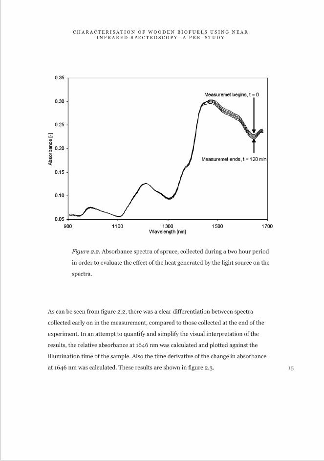
C H A R A C T E R I S A T I O N O F W O O D E N B I O F U E L S U S I N G N E A R I N F R A R E D S P E C T R O S C O P Y — A P R E – S T U D Y
Figure 2.2. Absorbance spectra of spruce, collected during a two hour period
in order to evaluate the effect of the heat generated by the light source on the
spectra.
As can be seen from figure 2.2, there was a clear differentiation between spectra
collected early on in the measurement, compared to those collected at the end of the
experiment. In an attempt to quantify and simplify the visual interpretation of the
results, the relative absorbance at 1646 nm was calculated and plotted against the
illumination time of the sample. Also the time derivative of the change in absorbance
at 1646 nm was calculated. These results are shown in figure 2.3.

16
R E P O R T
Figure 2.3. The relative change in absorbance at 1646 nm and the time
derivative of this change versus sample illumination time. The change in
absorbance is here contributed to the change in temperature generated by the
light source.
The conclusions that can be drawn from figure 2.3 are similar to that from figure
2.2, i.e. the temperature takes a long time to stabilise. Furthermore, the effect of the
change in temperature is significant, based on the fact that a four percent change in
absorbance at 1646 nm was observed in this study. This does not necessarily translate
into a four percent measurement error in the components of interest, but as such
the temperature effect can not be ignored. Based on the results from this study, the
following conclusions were made. Since the temperature effect cannot readily be
ignored, and the time required before temperature stability is reached is considerable,

17
C H A R A C T E R I S A T I O N O F W O O D E N B I O F U E L S U S I N G N E A R I N F R A R E D S P E C T R O S C O P Y — A P R E – S T U D Y
it seems appropriate to suggest that the measurement should be performed
directly after the sample is placed under the SentroHead, and the sample removed
directly after the measurement has been performed. This seems to be the optimal
measurement practice, and, considering that the measurement time for a 32 co–added
scans spectrum is roughly 8 seconds, the temperature effect should not be a significant
contributor in the spectral information.
2.2 THE EFFECTS OF SAMPLE INHOMOGENITY.
One major factor in characterising wood–based fuels with NIR–spectoscopy should be
the ability to differentiate species of trees commonly found if Finland from each other.
As a rule of thumb, common species in Finland have roughly the same energy content
measured in kJ/kg, but a significant difference is found when the energy content per
volume is compared. Thus, if the instrument is capable of determining the composition
of a fuel sample in terms of which species makes up the sample, and to what relative
amount, it seems probable that the energy content can be estimated as well. However,
a particular specie is perhaps not a well defined concept in terms of its corresponding
fingerprint in the NIR–region. The following experiment was conducted in order to
evaluate the minimum discrepancy that can be expected for Norwegian spruce.
The experiment was carried out as follows. Five locations, with no knags, on a
roughly one meter long board of Norwegian spruce were selected. A spectrum was
collected from every location, after which the procedure was repeated four times. This
way the repeability of the measurement compared to the variations due to the location
on the board could be evaluated. An average spectrum was computed for every location
and the standard deviation between the average spectra from the five locations was
computed for each point in the spectra. A similar standard deviation was computed for
the five spectra from each location. The results are shown in figure 2.4.
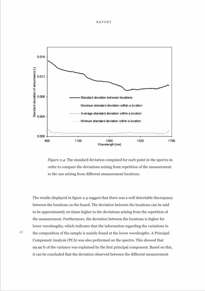
18
R E P O R T
Figure 2.4. The standard deviation computed for each point in the spectra in
order to compare the deviations arising from repetition of the measurement
to the one arising from different measurement locations.
The results displayed in figure 2.4 suggest that there was a well detectable discrepancy
between the locations on the board. The deviation between the locations can be said
to be approximately 20 times higher to the deviations arising from the repetition of
the measurement. Furthermore, the deviation between the locations is higher for
lower wavelengths, which indicates that the information regarding the variations in
the composition of the sample is mainly found at the lower wavelengths. A Principal
Component Analysis (PCA) was also performed on the spectra. This showed that
99.99 % of the variance was explained by the first principal component. Based on this,
it can be concluded that the deviation observed between the different measurement
19
C H A R A C T E R I S A T I O N O F W O O D E N B I O F U E L S U S I N G N E A R I N F R A R E D S P E C T R O S C O P Y — A P R E – S T U D Y
locations was due to changes in one particular spectral feature, rather than random
events. On the whole this study showed that in order to obtain a model that correctly
identifies Norwegian spruce, the model have to be trained on different samples of
this specie in order to account for the natural variations in the sample. Furthermore,
the NIR instrument can be said to have the capability to also measure at least one
component in Norwegian Spruce, although this component was not identified in this
experiment.
2.3 MOISTURE STABILITY OF THE SAMPLE
The moisture content of wooden biofuels is one very important parameter, both when
the biofuel is utilised (burned) and when it is purchased. NIRS measurements of water
can perhaps be said to be the most common application of NIR spectroscopy, and it
seems likely to assume that a reliable measurement can be obtained also for wooden
biofuels. However, one elementary issue has to be addressed. Since a wooden sample
with a moisture content of about 50 % is very far away from equilibrium with air during
any normal circumstances, the sample will dry at any time and anywhere. This means
that the sample has to be handled with some care, so that the reference measurement
and the NIR measurements actually represent the same moisture content. A simple
experiment was performed in order to evaluate the evaporation speed of water from a
piece of spruce board.
The piece of board had a surface area of approximately 560 cm² and a volume of
about 480 cm³. This piece of board is perhaps 5–10–fold larger than the average wood
chip size, which means that the relative water loss rate of wood chips is higher than in
this study. The piece of board was left to soak in water for one night, and the following
day the piece of board was weighted seven times at approximately one hour intervals.
During the time between weighting, the board piece was allowed to dry in room
temperature (approx. 22 °C), representing a typical laboratory measurement scenario.
Prior to the soaking, the board piece was weighted and this weight was used as dry
weight in the moisture content calculations. The reason for not drying the board piece
in an oven, which is the common procedure when determining the dry weight, was a
concern that the high temperature would alter the spectral features obtained from the

20
R E P O R T
board itself. The moisture content of the board as a function of drying time is shown in
figure 2.5.
Figure 2.5. The moisture content of a piece of board as a function of the
drying time in a normal indoor climate.
It is perhaps a matter of definition and sample handling procedure whether or not the
evaporation rate significantly affects the moisture content measurement. However,
NIR spectroscopy is a very effective way to measure water, which suggests that any
errors in the reference measurement could be significant. Based on the results in figure
2.5, the reference measurement and the NIR measurement should take place within
a time frame of minutes rather than half an hour. In particular when considering the
surface to volume ratio of the board piece in comparison to that of an average size
wood chip, it seems appropriate to suggest that the sample should be weighted either

21
C H A R A C T E R I S A T I O N O F W O O D E N B I O F U E L S U S I N G N E A R I N F R A R E D S P E C T R O S C O P Y — A P R E – S T U D Y
directly before or directly after the NIR measurement, directly meaning at least within
ten minutes.
However, it should be pointed out that moisture in wood can be separated into
two groups, depending of the place within the fibre structure that the water is located.
When the water is located within the straw–like structure of the wood–fibres it is
called “free water”. The remaining water is bound in the walls of the fibres and, thus,
referred to as “bound water”. When the free water has evaporated the remaining water
is essentially bound water, and this moisture content is called the “fibre saturation
point” According to a number mentioned in Rosner et al., 2009, this point corresponds
to a moisture content of 35–37 % in Norwegian spruce. In this study no further efforts
were made to confirm that these results regarding the evaporation rate, obtained on a
sample soaked in water, would also apply to samples of “green timber” (i.e. freshly cut
timber). However, if the moisture content of the sample is manipulated by adding fresh
water, it is advisory to perform the spectroscopic and reference measurement in an as
narrow as possible time frame.

22
R E P O R T
3. Distinguishability between common tree species
From the point of view of utilising wooden fuels for energy production, one important
parameter is without doubt the energy content. It was earlier suggested that the energy
content of wooden bio fuels is directly dependent on the composition of the fuel, i.e.
from which specie and from what part of the tree the fuel comes from. The following
study was conducted in order to evaluate the possibility to distinguish between “dry”
samples of birch, pine and spruce.
3.1 EXPERIMENTAL SETUP
The measurements were carried out on three roughly one meter long board pieces
of birch, spruce, and pine. The spectra were collected at randomly selected locations
of the board, covering the length of the board. Each spectrum consisted of 32
coadded scans. The spectrometer was allowed to stabilise for one hour prior to the
measurements. After this, ten spectra were collected from each board, one board at a
time. In order to reduce the influence of any time dependent factors, five more spectra
were collected from each board after the first series of measurement. Thus, 45 spectra
were collected for mathematical analysis, i.e. 15 from each board and specie. The
average spectrum from each specie is shown in figure 3.1.

23
C H A R A C T E R I S A T I O N O F W O O D E N B I O F U E L S U S I N G N E A R I N F R A R E D S P E C T R O S C O P Y — A P R E – S T U D Y
Figure 3.1. The average spectrum of birch, spruce, and pine computed from
15 spectra collected from three board pieces.
3.2 PRINCIPAL COMPONENT ANALYSIS
A visual inspection of figure 3.1 suggests that the spectrum from spruce and pine are
very similar to each other, whereas birch being a hardwood differs somewhat from the
two conifers. A PCA was performed on mean centred second order derivative spectra in
the region of 901–1301 nm. The derivative used was a 21 point second order Savitzky–
Golay derivative. Figure 3.2 shows the second principal component plotted against the
first principal component. One important conclusion that can be drawn from figure 3.2
is that spruce could not be distinguished from pine. This result is perhaps in conflict

24
R E P O R T
with some findings in the literature (Arshadi et al., 2007), but one explanation might
be that the boards from which the spectra were collected had been stored for some
time already. Therefore the spectra could perhaps be said to lack the information about
volatile compounds, and the information thus limited to cellulose and lignin content.
Figure 3.2. The second principal component plotted against the first principal
component. Results from PCA analysis of spectra collected from three
different wood species.
According to figure 1.2, the birch board was fairly homogenous, and the spectra from
birch can readily be distinguished from spectra from pine and spruce. The figure also
shows that the spruce board was homogenous in comparison to the pine board. These
observations can also be said to coincide with a visual evaluation of the boards. The
25
C H A R A C T E R I S A T I O N O F W O O D E N B I O F U E L S U S I N G N E A R I N F R A R E D S P E C T R O S C O P Y — A P R E – S T U D Y
cluster of the spruce spectra falls within the cluster from the pine spectra, and in this
sense it is impossible to distinguish spruce from pine. On the other hand, although the
information in the spectra from spruce and pine appears to be the same, the inhomo-
geneity of the pine board makes some spectra much more likely to be from pine than
from spruce. However, since the intention was to obtain quantitative measurements
utilising PLS models, the results from the PCA cannot be seen as conclusive. Among
other things, additional components in the model might accommodate for specie–
distinct features.
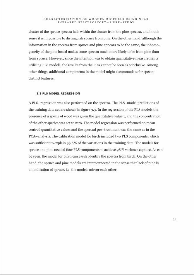
3.3 PLS MODEL REGRESSION
A PLS–regression was also performed on the spectra. The PLS–model predictions of
the training data set are shown in figure 3.3. In the regression of the PLS models the
presence of a specie of wood was given the quantitative value 1, and the concentration
of the other species was set to zero. The model regression was performed on mean
centred quantitative values and the spectral pre–treatment was the same as in the
PCA–analysis. The calibration model for birch included two PLS components, which
was sufficient to explain 99.6 % of the variations in the training data. The models for
spruce and pine needed four PLS components to achieve 98 % variance capture. As can
be seen, the model for birch can easily identify the spectra from birch. On the other
hand, the spruce and pine models are interconnected in the sense that lack of pine is
an indication of spruce, i.e. the models mirror each other.
26
R E P O R T
Figure 3.3. PLS model predictions of the composition of the spectra in the
training data set. A value of 1 indicates that the spectra comes from the specie
in question, otherwise the value should be zero.
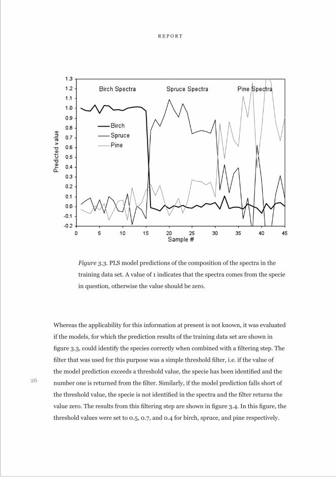
Whereas the applicability for this information at present is not known, it was evaluated
if the models, for which the prediction results of the training data set are shown in
figure 3.3, could identify the species correctly when combined with a filtering step. The
filter that was used for this purpose was a simple threshold filter, i.e. if the value of
the model prediction exceeds a threshold value, the specie has been identified and the
number one is returned from the filter. Similarly, if the model prediction falls short of
the threshold value, the specie is not identified in the spectra and the filter returns the
value zero. The results from this filtering step are shown in figure 3.4. In this figure, the
threshold values were set to 0.5, 0.7, and 0.4 for birch, spruce, and pine respectively.
27
C H A R A C T E R I S A T I O N O F W O O D E N B I O F U E L S U S I N G N E A R I N F R A R E D S P E C T R O S C O P Y — A P R E – S T U D Y
Figure 3.4. Filtered PLS model predictions of the composition of the spectra
in the training data set. A value of 1 indicates that the spectra comes from the
specie in question, otherwise the value should be zero.
Whereas the results in figure 3.4 shows a perfect prediction of every sample or spectra
in the training data set, it was decided that the models should also be validated
against data detached from the model regression, i.e. against a validation set. For this
purpose additional spectra were collected from three boards from the three species.
These boards were not the same ones that were used for the model regression, and the
collection of the spectra took place one week after the collection of the training data
set. Thus, this experiment aimed to verify whether or not the NIR spectrometer could
be used for identifying boards from birch, spruce and pine. From each board 15 new
spectra were collected in a similar manner to the training data set. The models were
28
R E P O R T
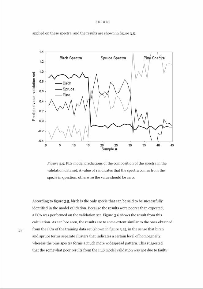
applied on these spectra, and the results are shown in figure 3.5.
Figure 3.5. PLS model predictions of the composition of the spectra in the
validation data set. A value of 1 indicates that the spectra comes from the
specie in question, otherwise the value should be zero.
According to figure 3.5, birch is the only specie that can be said to be successfully
identified in the model validation. Because the results were poorer than expected,
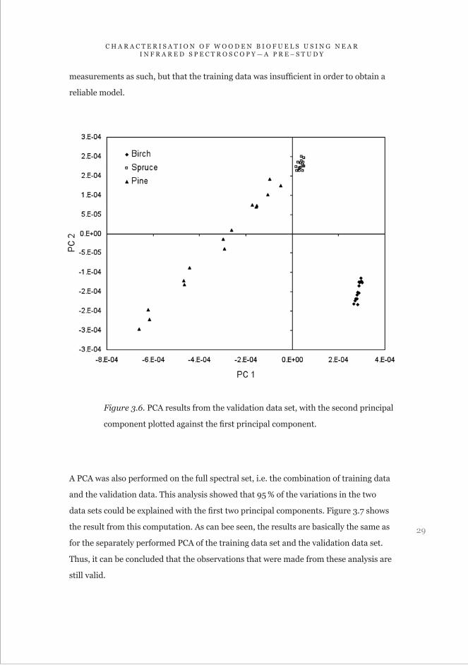
a PCA was performed on the validation set. Figure 3.6 shows the result from this
calculation. As can bee seen, the results are to some extent similar to the ones obtained
from the PCA of the training data set (shown in figure 3.2), in the sense that birch
and spruce forms separate clusters that indicates a certain level of homogeneity,
whereas the pine spectra forms a much more widespread pattern. This suggested
that the somewhat poor results from the PLS model validation was not due to faulty
29
C H A R A C T E R I S A T I O N O F W O O D E N B I O F U E L S U S I N G N E A R I N F R A R E D S P E C T R O S C O P Y — A P R E – S T U D Y
measurements as such, but that the training data was insufficient in order to obtain a
reliable model.
Figure 3.6. PCA results from the validation data set, with the second principal
component plotted against the first principal component.
A PCA was also performed on the full spectral set, i.e. the combination of training data
and the validation data. This analysis showed that 95 % of the variations in the two
data sets could be explained with the first two principal components. Figure 3.7 shows
the result from this computation. As can bee seen, the results are basically the same as
for the separately performed PCA of the training data set and the validation data set.
Thus, it can be concluded that the observations that were made from these analysis are
still valid.

30
R E P O R T
Figure 3.7. PCA results from the combination of the training data set and the
validation data set, with the second principal component plotted against the
first principal component.
As a final investigation in the present study of differentiation between three species,
PLS models were computed and validated on combinations of the original training
data and validation set. The training data set for this study was based on ten spectra
from each specie from the original training data set, and ten spectra from the original
validation data set. The remaining spectra were used for model validation. Thus, the
models were based on 60 spectra and the validation carried out on 30 spectra. With
two PLS components for the birch PLS model, 99 % of the variations in the training
data was explained. In the case of spruce and pine, six PLS components yielded into
31
C H A R A C T E R I S A T I O N O F W O O D E N B I O F U E L S U S I N G N E A R I N F R A R E D S P E C T R O S C O P Y — A P R E – S T U D Y
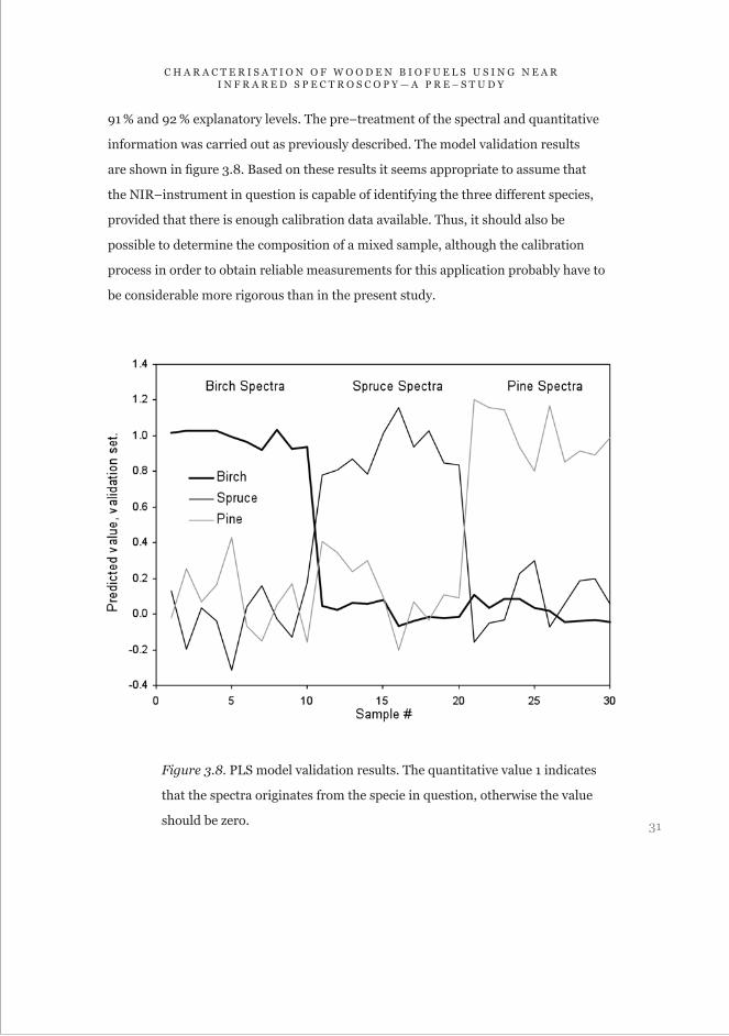
91 % and 92 % explanatory levels. The pre–treatment of the spectral and quantitative
information was carried out as previously described. The model validation results
are shown in figure 3.8. Based on these results it seems appropriate to assume that
the NIR–instrument in question is capable of identifying the three different species,
provided that there is enough calibration data available. Thus, it should also be
possible to determine the composition of a mixed sample, although the calibration
process in order to obtain reliable measurements for this application probably have to
be considerable more rigorous than in the present study.
Figure 3.8. PLS model validation results. The quantitative value 1 indicates
that the spectra originates from the specie in question, otherwise the value
should be zero.

32
R E P O R T
Regardless of whether the information displayed in figure 3.8 should be seen as
successful implementation or not, some observations can be made. Firstly, the type
of filtering used on the results displayed in figure 3.4 can not be directly applied
to mixtures of wood, which makes it an infeasible approach for wooden biofuel
measurements. However, figure 3.8 indicates that a quantitative and reliable PLS
model might also be obtainable. Secondly, if fresh pine and spruce forms clear and
separated cluster on the second PC vs. first PC (Arshadi et al., 2007), these results,
in combination with the results from this study, indicates that a significant change
in the spectra will occur during the seasoning of the timber. Consequently, if the fuel
at the time of measurement contains various amounts of volatile substances, the
mathematical model that is used to predict the fuels properties have to be robust to the
changes in these substances as well. Therefore it can perhaps be said that this study
answered some questions, but also gave rise to new factors to be considered.

33
C H A R A C T E R I S A T I O N O F W O O D E N B I O F U E L S U S I N G N E A R I N F R A R E D S P E C T R O S C O P Y — A P R E – S T U D Y
4. Measurement of the moisture content
As earlier stated, the moisture content is perhaps the most important parameter
when defining solid biofuel properties. As a reminder, the moisture content is in
this study defined as water to total weight ratio. However, regardless if the moisture
content is defined as the ratio of water to total weight, or water to dry weight, the
reference measurements can be carried out with basic laboratory equipment, i.e.
weighting–drying–weighting. On the other hand, from the NIR measurement point
of view moisture content is perhaps not an uncomplicated parameter. Basically the
signal received with NIR spectroscopy should contain the information about how many
water molecules the beam has encountered before reaching the detector. The number
of water molecules the beam will interact with before reaching the detector has to be
dependent on the volumetric density of the water in the sample and the length the light
travels through the sample before it is reflected back to the detector. The moisture
content as a parameter is dependent on the mass, and therefore also on the density, of
the dry substance. The question is how much the density of the dry substance affects
the NIR measurement of water.
It can be assumed that the different densities of solid biofuels, or in this case
common Finnish tree species, will affect the measurement. For a given volumetric
water concentration, a fuel with a low density will have a higher moisture content
than a fuel with a high density. In other words, if the NIR signal is equivalent to the
amount of water in the sample, some precautionary steps are needed when attempting
to measure the moisture content of fuels with different densities. An additive effect
can also perhaps be expected with the NIR measurements based on the following
reasoning. It could be assumed that the light travels a longer distance in a wood with
low density, before being reflected back to the detector. This would give a stronger
water absorbance in the spectra and add to the effect from the density dependent
definition of moisture content.
The measurements presented in this section where performed on a piece of board
and can therefore be seen as a considerable simplification compared to measurements
on wood chips and various forms of wooden biofuel materials. Perhaps this study can
34
R E P O R T
be said to represents a reasonable “best case scenario”, or the simplest experimental
setup for NIR spectroscopic measurements of moisture content in solid biofuels.
However, since the board piece by no means should be described as a homogenous
background, a PLS model for the moisture content has to be able to account for
spectral features arising from the board piece itself. Furthermore, it can be assumed
that the water is not entirely homogenously distributed in the board piece, due to a
supposed local variance in hygroscopic nature of the wood. Another potential issue is
concentration gradients arising from the surface evaporation. It can be assumed that
if the water is uniformly spread in the body at the time when evaporation starts, there
can be concentration gradients between the surface and the inner parts of the sample.
4.1 EXPERIMENTAL SETUP
The NIR spectroscopic measurement of moisture content was carried out on the same
piece of board as in the study described in section 2.3. The basic approach was to
soak the board piece in water for one night, and allow it to dry in room temperature
after this. During the drying time the board piece was weighted several times, and for
each weighting 10 spectra were collected at different locations on the board piece (five
from each side). Each spectrum consisted of 32 co–added scans, and the integration
time was 0.16 seconds. The spectra were collected from the region 905–1683 nm,
and recorded at a 3 nm step size. Altogether 180 spectra were collected for analysis,
and the moisture content of these samples ranged from 4 to 29 %. However, it
should be pointed out that the moisture content values given in this study does not
fully agree with the definition of moisture content, because the board piece was not
dried according to standards (e.g. ISO 287:2009) in order to obtain the dry weight.
Instead the dry weight of the sample was considered to be the weight of the sample in
equilibrium with the indoor air at the time of the measurements. This approach was
taken due to a concern that the heating of the sample in an oven, in accordance with
standard measurement methods for moisture content, would affect the NIR signal
from the board piece itself. After the study described here was completed, the board
piece was dried for 2 months in an exicator. The dry weight measured after this period
was 4 % lower than the one that was used to produce the data given in this report.

35
C H A R A C T E R I S A T I O N O F W O O D E N B I O F U E L S U S I N G N E A R I N F R A R E D S P E C T R O S C O P Y — A P R E – S T U D Y
4.2 PRINCIPAL COMPONENT ANALYSIS
The first evaluation of the measurements was done with PCA. For the PCA the whole
measured wavelength region was utilized, and the only pre–processing method was
mean centring. As earlier indicated, the spectra representing one level of moisture
content did vary significantly from at least a visual point of view. In addition, it can
be said that as the moisture content decreased, the relative discrepancy between
spectra representing a single moisture content value increased. This as a direct result
of that the relative influence of the background matrix increases as the water features
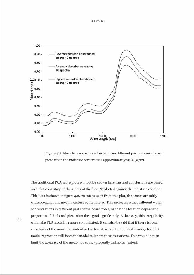
decreases in magnitude. Figure 4.1 shows three spectra, all of which represent the
same moisture content (29 %). According to the figure, the absorbance is reaching 1,
and severe nonlinearities were expected. However, the PCA on the 180 spectra showed
that 95.8 % of the variations could be explained by the first PC, and 4 % with the second
PC. Thus, 99.8 of all variations were explained with only two PC. Perhaps it can be
assumed that in this case the first PC can be directly related to the water content and
the second mainly with features arising from the inhomogenity of the board piece.
36
R E P O R T
Figure 4.1. Absorbance spectra collected from different positions on a board
piece when the moisture content was approximately 29 % (w/w).
The traditional PCA score plots will not be shown here. Instead conclusions are based
on a plot consisting of the scores of the first PC plotted against the moisture content.
This data is shown in figure 4.2. As can be seen from this plot, the scores are fairly
widespread for any given moisture content level. This indicates either different water
concentrations in different parts of the board piece, or that the location dependent
properties of the board piece alter the signal significantly. Either way, this irregularity
will make PLS modelling more complicated. It can also be said that if there is local
variations of the moisture content in the board piece, the intended strategy for PLS
model regression will force the model to ignore these variations. This would in turn
limit the accuracy of the model too some (presently unknown) extent.
37
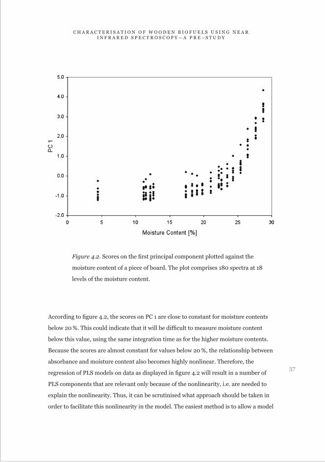
C H A R A C T E R I S A T I O N O F W O O D E N B I O F U E L S U S I N G N E A R I N F R A R E D S P E C T R O S C O P Y — A P R E – S T U D Y
Figure 4.2. Scores on the first principal component plotted against the
moisture content of a piece of board. The plot comprises 180 spectra at 18
levels of the moisture content.
According to figure 4.2, the scores on PC 1 are close to constant for moisture contents
below 20 %. This could indicate that it will be difficult to measure moisture content
below this value, using the same integration time as for the higher moisture contents.
Because the scores are almost constant for values below 20 %, the relationship between
absorbance and moisture content also becomes highly nonlinear. Therefore, the
regression of PLS models on data as displayed in figure 4.2 will result in a number of
PLS components that are relevant only because of the nonlinearity, i.e. are needed to
explain the nonlinearity. Thus, it can be scrutinised what approach should be taken in
order to facilitate this nonlinearity in the model. The easiest method is to allow a model

38
R E P O R T
with a high number of PLS components. This approach requires no extra effort in the
regression of the model. However, although it is not readily quantifiable or verifiable,
it seems appropriate to suggest that the higher the number of PLS components that are
required the less robust the model will be to spectra features that are not accounted for
in the training data, but that potentially could arise in prediction spectra.
4.3 PLS MODELS REGRESSION, AND METHODS TO ACCOUNT FOR NON–LINEARITY
If an attempt to decrease the number of PLS components needed in the PLS models
predicting the moisture content seems as a favourable approach, there are at least
two fairly easily implementable options. The first one is to create several separate
calibration models, covering different moisture content intervals, in which the
relationship between absorbance and moisture is sufficiently linear. The downside
with this approach is that the training data set for each model will decrease in size,
which in one sense is a waste of available information and might reduce the robustness
of the model. Again, no clear values can be given to how the size of the training data
set affects the quality of the PLS model, but it seems reasonable to suggest that, as
a rule of thumb, a larger training data set should make the model more robust and
thereby more accurate. The second approach is to transform the quantitative data,
in order to make the relation between the quantitative value, i.e. the transformation
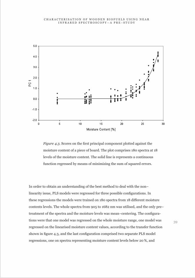
of the moisture content, and the spectral response linear. Figure 4.3 shows a transfer
function that was used in order to evaluate the potential benefits of a linearization.
This transfer function was obtained by making a least squares function fit between the
scores on the first principal component and the moisture content values. The function
represents a linear relation up to 20 % moisture, and an exponential relationship is
used for values above 20 %. The parameters for the two functions were obtained by
minimizing the sum of squared errors.
39
C H A R A C T E R I S A T I O N O F W O O D E N B I O F U E L S U S I N G N E A R I N F R A R E D S P E C T R O S C O P Y — A P R E – S T U D Y
Figure 4.3. Scores on the first principal component plotted against the
moisture content of a piece of board. The plot comprises 180 spectra at 18
levels of the moisture content. The solid line is represents a continuous
function regressed by means of minimizing the sum of squared errors.
In order to obtain an understanding of the best method to deal with the non–
linearity issue, PLS models were regressed for three possible configurations. In
these regressions the models were trained on 180 spectra from 18 different moisture
contents levels. The whole spectra from 905 to 1682 nm was utilised, and the only pre–
treatment of the spectra and the moisture levels was mean–centering. The configura-
tions were that one model was regressed on the whole moisture range, one model was
regressed on the linearised moisture content values, according to the transfer function
shown in figure 4.3, and the last configuration comprised two separate PLS model
regressions, one on spectra representing moisture content levels below 20 %, and
40
R E P O R T
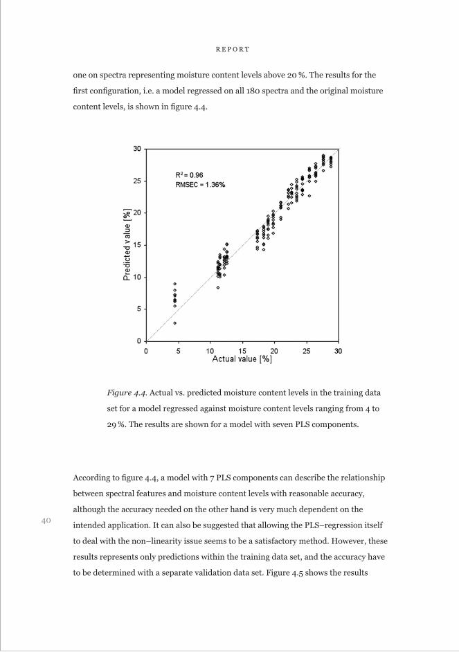
one on spectra representing moisture content levels above 20 %. The results for the
first configuration, i.e. a model regressed on all 180 spectra and the original moisture
content levels, is shown in figure 4.4.
Figure 4.4. Actual vs. predicted moisture content levels in the training data
set for a model regressed against moisture content levels ranging from 4 to
29 %. The results are shown for a model with seven PLS components.
According to figure 4.4, a model with 7 PLS components can describe the relationship
between spectral features and moisture content levels with reasonable accuracy,
although the accuracy needed on the other hand is very much dependent on the
intended application. It can also be suggested that allowing the PLS–regression itself
to deal with the non–linearity issue seems to be a satisfactory method. However, these
results represents only predictions within the training data set, and the accuracy have
to be determined with a separate validation data set. Figure 4.5 shows the results

41
C H A R A C T E R I S A T I O N O F W O O D E N B I O F U E L S U S I N G N E A R I N F R A R E D S P E C T R O S C O P Y — A P R E – S T U D Y
for the model regressed against linearised moisture content values. As was earlier
mentioned, and as can be seen from figure 4.3, the variance of the transformed
moisture content representing values lower than 20 % is very small. The effects of this
can be seen in figure 4.5.
Figure 4.5. Actual vs. predicted moisture content levels in the training data
set, for a model regressed against linearised moisture content levels
representing original values from 4 to 29 %, after retransformation of the
moisture content values. The results are shown for a model with two PLS
components. The original PLS model predictions on the linearised, i.e. the
transformed, values are also shown.
There are some conclusions that can be drawn from figure 4.5. There appears to be
some benefits with this method of linearization for higher moisture content values,
in particular when 25 % is exceeded. Comparing figure 4.5 and 4.4 shows that the
42
R E P O R T
predictions are more consistent for the model regressed on linearized moisture values.
Furthermore, the more accurate predictions are obtained with a model with only two
PLS components. However, at values below 20 % the model or method is useless. This
result can be contributed to the very small changes in the values obtained from the
transfer function for values below 20 %, as illustrated in figure 4.3. As can be seen from
figure 4.5, the PLS model predicts the low linearized values fairly well, but the errors
are multiplied by a factor of approximately 100 with the transfer function, resulting
in a worthless method. It would be possible to increase the variance for values below
20 % by increasing the angle of the line describing the linear part of the relationship,
but then the relationship between the first PCA and the transformed values would no
longer be linear and linearization in this sense less powerful. Thus, this approach for
linearization is a method of interest only if it is used in the regression of a model that
describes moisture content values above 20 %. However, with this limitation in place, a
reasonable model can be obtained already with only two PLS components.
The third and final configuration that was evaluated was a two model approach,
one for concentrations below 20 % and one for concentrations above 20 %. The results
are shown in figure 4.6. As earlier discussed, the robustness of the models might be an
issue but, as can be seen from the figure, the predictions of the moisture in the spectra
of the training data set are fairly accurate. Based on the correlation and the standard
error obtained with this approach, this approach seems like the best alternative from
the three configurations studied. However, this result has to be validated before the
final conclusions can be drawn. It is perhaps no surprise that decreasing the moisture
content interval that the model has to account for, increases the accuracy of the
predictions within the training data set. The question is how the decrease in the size of
the training data set, compared to using all data for model regression, affects the model
robustness. Furthermore, if several models are to be utilised for the measurement,
there has to be an approach that determines which prediction will represent the actual
measurement result, i.e. which model should be used. Therefore a validation is needed
in order to establish the best approach. However, some conclusions can be drawn
already from this study. Linearization implemented as in this study is to be used,
if used at all, only at higher moisture content levels, i.e. when the spectral features
are dominated by water. It might be favourable to use two calibration models when
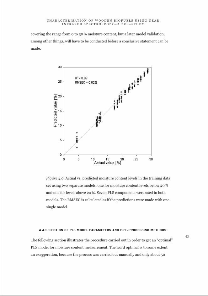
43
C H A R A C T E R I S A T I O N O F W O O D E N B I O F U E L S U S I N G N E A R I N F R A R E D S P E C T R O S C O P Y — A P R E – S T U D Y
covering the range from 0 to 30 % moisture content, but a later model validation,
among other things, will have to be conducted before a conclusive statement can be
made.
Figure 4.6. Actual vs. predicted moisture content levels in the training data
set using two separate models, one for moisture content levels below 20 %
and one for levels above 20 %. Seven PLS components were used in both
models. The RMSEC is calculated as if the predictions were made with one
single model.
4.4 SELECTION OF PLS MODEL PARAMETERS AND PRE–PROCESSING METHODS
The following section illustrates the procedure carried out in order to get an “optimal”
PLS model for moisture content measurement. The word optimal is to some extent
an exaggeration, because the process was carried out manually and only about 50

44
R E P O R T
models were calculated, whereas the number of possible regression setups is, from a
manual approach point of view, almost unlimited. The methodology used and the best
model regression setup found can, as such, not be perceived as a generally applicable
method or truth, because all applications are unique. However, the data shown can
serve as an example on the importance of finding the proper model parameters and
pre–processing methods. The PLS models that are characterised in this section were
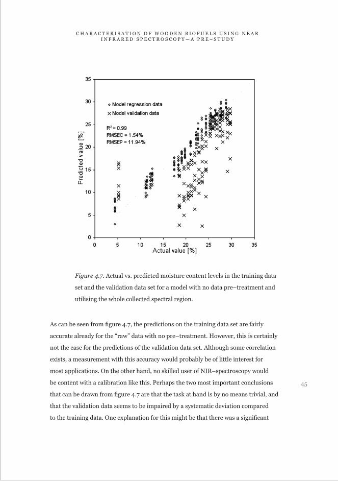
regressed on the spectra collected as described in section 4.1. In order to validate the
models the piece of board was soaked in water one more time, and 160 new spectra
were collected for 16 new moisture content levels the same way as described in section
4.1. The start point for this study was a model regressed on the whole spectral region
collected, and with no pre–treatment. The predictions of the training data set and the
validation data set are shown in figure 4.7.
45
C H A R A C T E R I S A T I O N O F W O O D E N B I O F U E L S U S I N G N E A R I N F R A R E D S P E C T R O S C O P Y — A P R E – S T U D Y
Figure 4.7. Actual vs. predicted moisture content levels in the training data
set and the validation data set for a model with no data pre–treatment and
utilising the whole collected spectral region.
As can be seen from figure 4.7, the predictions on the training data set are fairly
accurate already for the “raw” data with no pre–treatment. However, this is certainly
not the case for the predictions of the validation data set. Although some correlation
exists, a measurement with this accuracy would probably be of little interest for
most applications. On the other hand, no skilled user of NIR–spectroscopy would
be content with a calibration like this. Perhaps the two most important conclusions
that can be drawn from figure 4.7 are that the task at hand is by no means trivial, and
that the validation data seems to be impaired by a systematic deviation compared
to the training data. One explanation for this might be that there was a significant

46
R E P O R T
dark coloured fungal growth occurring on the board piece during the collection of the
validation data set, which certainly had some impact also on the spectra collected.
Figure 4.8. The root mean square error of calibration, the correlation
coefficient squared, and the root mean square error of prediction for 37 PLS
models regressed and validated on the same data, but with different setups on
the model regression parameters and spectral pre–treatment methods.
The model regression setups that yielded in the information presented in figure 4.8 will
not be presented in great detail. However, a brief description is needed. The dramatic
improvement observable for the first and second regression (the regression shown in
figure 4.7 is regarded as regression number zero) is obtained by first mean centring
and then auto scaling the spectra. The moisture content values were mean centred
as well. After this, the spectrum interval that the models regressions were performed
47
C H A R A C T E R I S A T I O N O F W O O D E N B I O F U E L S U S I N G N E A R I N F R A R E D S P E C T R O S C O P Y — A P R E – S T U D Y
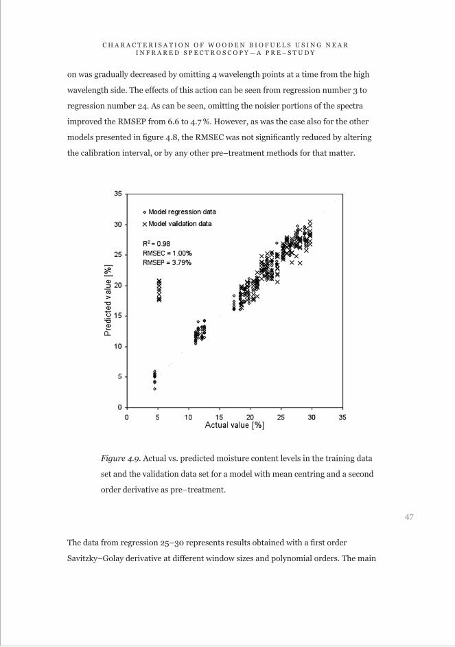
on was gradually decreased by omitting 4 wavelength points at a time from the high
wavelength side. The effects of this action can be seen from regression number 3 to
regression number 24. As can be seen, omitting the noisier portions of the spectra
improved the RMSEP from 6.6 to 4.7 %. However, as was the case also for the other
models presented in figure 4.8, the RMSEC was not significantly reduced by altering
the calibration interval, or by any other pre–treatment methods for that matter.
Figure 4.9. Actual vs. predicted moisture content levels in the training data
set and the validation data set for a model with mean centring and a second
order derivative as pre–treatment.
The data from regression 25–30 represents results obtained with a first order
Savitzky–Golay derivative at different window sizes and polynomial orders. The main

48
R E P O R T
change when using derivative as pre–treatment is found in the correlation values.
This is particularly true for regression 31–37, where a second order Savitzky–Golay
derivative was tried out for a second order polynomial with different window sizes.
On the whole, the use of the derivative as pre–treatment did not improve the RMSEP
that significantly, i.e. from 4.7 % to 3.8 %, but since it was an improvement that also
increased the correlation, it was decided that mean centring combined with a second
order derivative will be the standard pre–treatment for future model development.
Figure 4.9 shows the predictions of the training data set and validation data set, for
a model regressed with mean centring and second order derivative as pre–treatment
(regression number 35 in figure 4.8). According to the results from section 4.3, there is
a potential for model improvement by creating several models where each model only
describes a portion of the measured moisture content interval. It was also suggested
that a method of linearization could be of interest, provided that it was performed on
a narrower moisture content interval. Thus, this was the subject of further investiga-
tions.
4.5 LOCAL PLS MODELS AND LOCAL LINEARIZATION
The starting point for the evaluation of the usefulness of local PLS models, for different
portions of the moisture content interval, was a model regressed on mean centered,
second order Savitzky–Golay derivative spectra. As concluded in the previous section
the RMSEP for this model was 3.8 %. However, for the purpose of comparison of
local models to the macro model, the RMSEP was recalculated treating the validation
sample at approximately 5 % moisture content as an outlier. As can be seen in figure
4.9 this sample was clearly an outlier. Thus, the measurement accuracy that the local
models could be compared to is 1.48 %, obtained after excluding the outlier, rather
than 3.8 % as previously reported. However, as can be seen from for instance figure
4.9, the previously utilized validation data set had only a few validation points below
20 %, and one of which was an outlier. In order to evaluate the accuracy for local
models below 20 % an additional validation data set was collected. The procedure was
the same as for the earlier data set, i.e. the board piece was soaked in water over night,
and new spectra were collected while the board piece was drying. Thus, the evaluation

49
C H A R A C T E R I S A T I O N O F W O O D E N B I O F U E L S U S I N G N E A R I N F R A R E D S P E C T R O S C O P Y — A P R E – S T U D Y
of the usability of local PLS models was conducted on a validation data set, that was a
combination of the original and the new validation data set.
The new validation data set collected contained only moisture content levels
below 20 %, and the models regressed for higher moisture content values were
therefore in practice validated against the first or original validation data set. However,
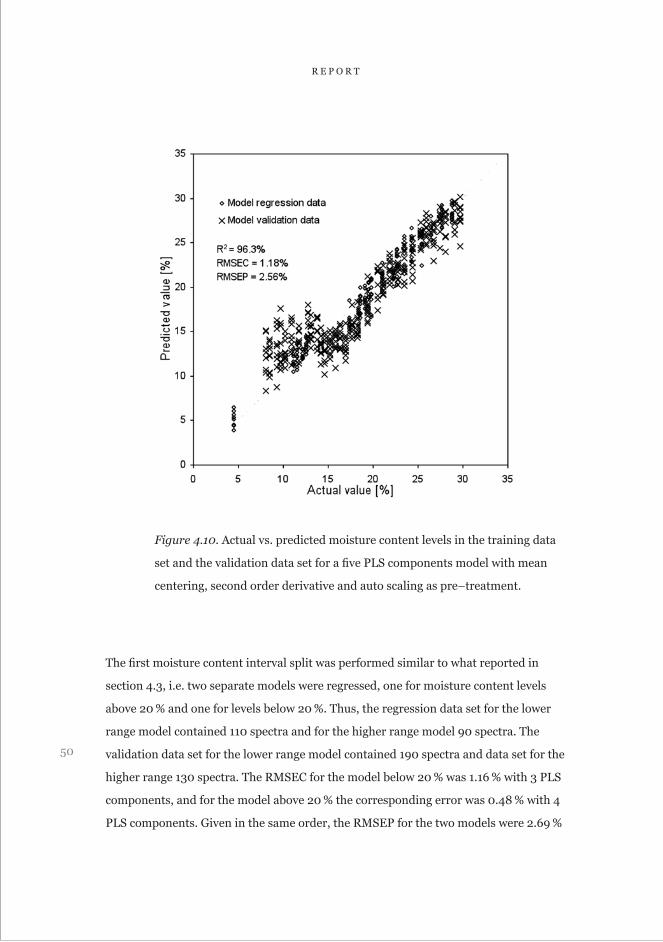
for the purpose of further investigations, the regression and validation data set can be
described as follows. The regression data set in the following calculations consist of
200 spectra, representing 20 different moisture content levels. These spectra are from
the original regression set (180), and spectra from the first validation data set that
represent moisture contents below 20 %. The validation data set consist of 320 spectra,
representing 32 moisture content levels. These spectra come from the original or first
validation data set (130), representing moisture content levels above 20 %, and the new
validation data set (190 spectra). A model regression and validation was performed
with the above described training data set and validation data set. The pre treatment
utilized was mean centering, a second order Savitzky–Golay derivative with a second
order polynomial and a 13 point window size, and auto scaling. The results from this
regression and validation are shown in figure 4.10.
50
R E P O R T
Figure 4.10. Actual vs. predicted moisture content levels in the training data
set and the validation data set for a five PLS components model with mean
centering, second order derivative and auto scaling as pre–treatment.
The first moisture content interval split was performed similar to what reported in
section 4.3, i.e. two separate models were regressed, one for moisture content levels
above 20 % and one for levels below 20 %. Thus, the regression data set for the lower
range model contained 110 spectra and for the higher range model 90 spectra. The
validation data set for the lower range model contained 190 spectra and data set for the
higher range 130 spectra. The RMSEC for the model below 20 % was 1.16 % with 3 PLS
components, and for the model above 20 % the corresponding error was 0.48 % with 4
PLS components. Given in the same order, the RMSEP for the two models were 2.69 %
51
C H A R A C T E R I S A T I O N O F W O O D E N B I O F U E L S U S I N G N E A R I N F R A R E D S P E C T R O S C O P Y — A P R E – S T U D Y
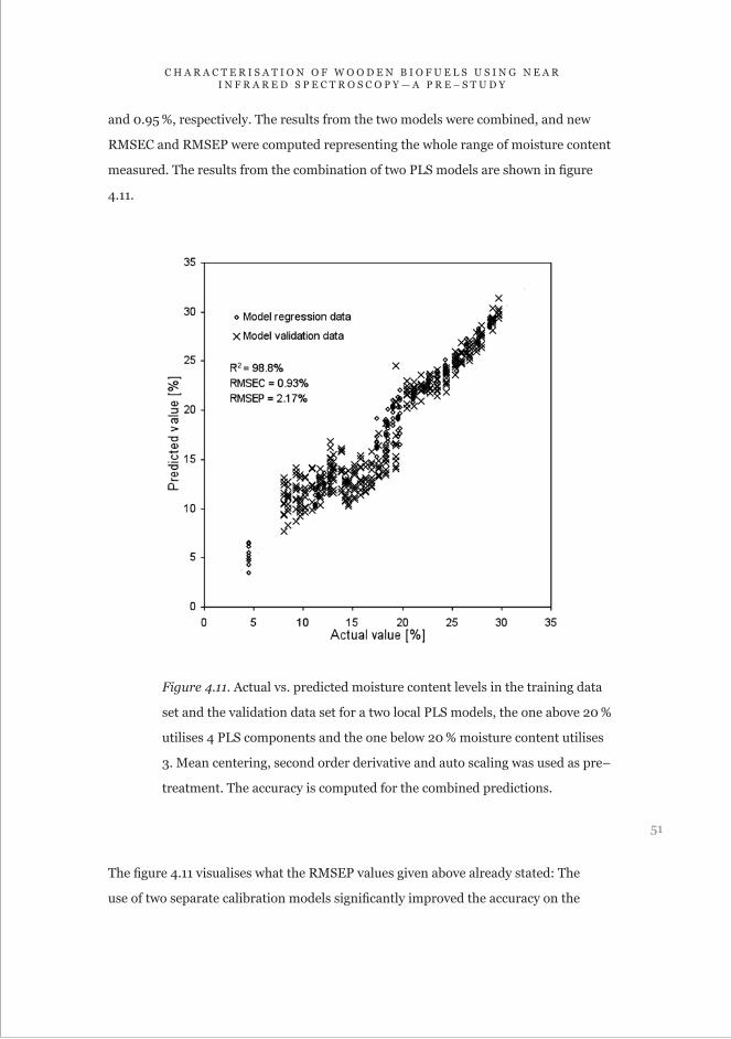
and 0.95 %, respectively. The results from the two models were combined, and new
RMSEC and RMSEP were computed representing the whole range of moisture content
measured. The results from the combination of two PLS models are shown in figure
4.11.
Figure 4.11. Actual vs. predicted moisture content levels in the training data
set and the validation data set for a two local PLS models, the one above 20 %
utilises 4 PLS components and the one below 20 % moisture content utilises
3. Mean centering, second order derivative and auto scaling was used as pre–
treatment. The accuracy is computed for the combined predictions.
The figure 4.11 visualises what the RMSEP values given above already stated: The
use of two separate calibration models significantly improved the accuracy on the

52
R E P O R T
measurements above 20 % moisture content level, but did not affect the accuracy
below 20 % to any greater extent. It should be pointed out that the validation data
for the model below 20 % was obtained as a separate measurement series, collected
a few days after the first validation data set. As previously mentioned, the board
piece became gradually darker during the measurements due to fungal growth. This
might be an explanation to why the model fails to predict the concentrations in the
second validation set with the same accuracy as for the first set. If the fungal growth
significantly affected the spectra of the second validation data set, and the model was
regressed on spectra with very little influence of fungal growth, the model cannot
account for features that were not included in the training data. As a consequence,
it can not be evaluated if the use of local models improved the measurement below
20 % at this point. On the other hand, the improvement above 20 % was significant,
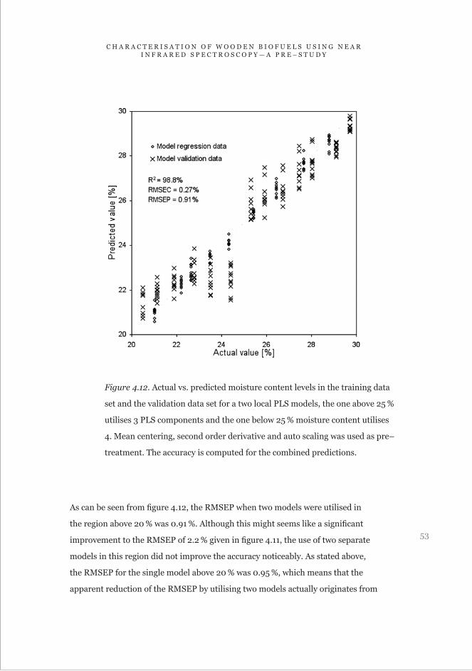
and therefore one more interval split was performed. Two new models were regressed
for the interval above 20 %, one on spectra ranging between 20 to 25 %, and one on
spectra above 25 %. The results from the model regressions and validations are shown
in figure 4.12.
53
C H A R A C T E R I S A T I O N O F W O O D E N B I O F U E L S U S I N G N E A R I N F R A R E D S P E C T R O S C O P Y — A P R E – S T U D Y
Figure 4.12. Actual vs. predicted moisture content levels in the training data
set and the validation data set for a two local PLS models, the one above 25 %
utilises 3 PLS components and the one below 25 % moisture content utilises
4. Mean centering, second order derivative and auto scaling was used as pre–
treatment. The accuracy is computed for the combined predictions.
As can be seen from figure 4.12, the RMSEP when two models were utilised in
the region above 20 % was 0.91 %. Although this might seems like a significant
improvement to the RMSEP of 2.2 % given in figure 4.11, the use of two separate
models in this region did not improve the accuracy noticeably. As stated above,
the RMSEP for the single model above 20 % was 0.95 %, which means that the
apparent reduction of the RMSEP by utilising two models actually originates from

54
R E P O R T
excluding the validation data below 20 % moisture content level. However, it can be
said that the RMSEP for the model above 25 % was 0.65 %, which can be seen as a
significant improvement compared to the previously obtained 0.95 %. On the other
hand, if a RMSEP for the measurement shown in figure 4.11 is calculated only for the
measurements above 25 %, this error amounts to 0.56 %. Thus, it can be concluded
that the use of two models in the region 20 to 30 % moisture content level can not
be considered an improvement compared to using only one model. However, this
result should not bee seen as a generally applicable conclusion, because every split
in regression interval also implied a significant reduction of the training data set.
Hence, it can be suggested that the use of local models can be recommended if there
is sufficient training data available for each model. Therefore, as is the case in most
applications, the accuracy that can be achieved is highly dependent on the amount of
representative training data that is available.
55
C H A R A C T E R I S A T I O N O F W O O D E N B I O F U E L S U S I N G N E A R I N F R A R E D S P E C T R O S C O P Y — A P R E – S T U D Y
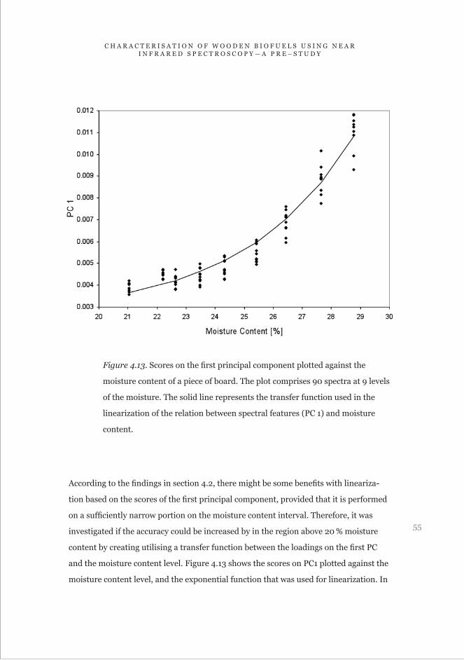
Figure 4.13. Scores on the first principal component plotted against the
moisture content of a piece of board. The plot comprises 90 spectra at 9 levels
of the moisture. The solid line represents the transfer function used in the
linearization of the relation between spectral features (PC 1) and moisture
content.
According to the findings in section 4.2, there might be some benefits with lineariza-
tion based on the scores of the first principal component, provided that it is performed
on a sufficiently narrow portion on the moisture content interval. Therefore, it was
investigated if the accuracy could be increased by in the region above 20 % moisture
content by creating utilising a transfer function between the loadings on the first PC
and the moisture content level. Figure 4.13 shows the scores on PC1 plotted against the
moisture content level, and the exponential function that was used for linearization. In

56
R E P O R T
the first regression, the model was based on the 90 available spectra and correspond-
ing linearized moisture content data. The model was tested against the validation data
available for moisture content levels above 20 %, i.e. 130 spectra corresponding to 13
moisture content levels. This regression produced a model with a RMSEP of 1.75 %,
which is significantly higher than the RMSEP of 0.95 % obtained above 20 % with no
linearization.
One reason for the unsatisfactory result was the prediction errors in the lower
moisture content region. In order to compensate for the small variance of the concen-
tration data in this region, the training data set was modified. A new training data set
was created, in which the sample with the highest moisture content was included once,
the sample with the second highest moisture content twice, and so forth. However,
it should be pointed out that mean centering was used on the concentration data,
which to some extent counteracted this procedure to put more weight on the low
moisture content samples. This training data set consequently contained 450 spectra
representing 9 moisture content levels. The results from the regression can be seen in
figure 4.14. It was concluded, based on the RMSEP of 1.0 % obtained with this model,
that the efforts to linearize the regression data this way were pointless. The accuracy
obtained was the same as with no linearization, and therefore the whole approach as
such can be seen as a failure. Thus, for future applications it seems as a favourable
approach to use multiple local models for moisture content measurements, although
selecting the correct model for the measurement will be an issue. Furthermore, a
measurement accuracy of 1 % was obtained, which qualitatively can be described as a
reasonable, or perhaps even excellent, accuracy when dealing with characterisation of
wooden biofuels.

57
C H A R A C T E R I S A T I O N O F W O O D E N B I O F U E L S U S I N G N E A R I N F R A R E D S P E C T R O S C O P Y — A P R E – S T U D Y
Figure 4.14. Actual vs. predicted moisture content levels in the training data
set and the validation data set for a model regressed on linearized moisture
content values.
58
R E P O R T
5. Summary
In this report fundamental aspects of NIR spectroscopic characterization of wooden
biofuels were evaluated. The attempt was to investigate seemingly trivial matters, such
as heat generated by the light source and evaporation rate of water. As such, the results
are of practical rather than scientific importance. Regarding the heating effect that
the light source generates, the conclusion was that the impact was significant and that
the time required to obtain a reasonable stability was in the region of one hour. Thus,
it was suggested that the measurement head should be brought onto the sample as
shortly as possible before the measurement begins and removed as quickly as possible
after the spectra has been collected. Due to the short measurement time required to
collect a spectrum, the effect of the heat generated by the light source can sufficiently
be reduced by the proper handling of the measurement head. This investigation also
showed that the evaporation rate from a wooden sample, which has been soaked in
water to manipulate the moisture content, is in laboratory conditions high enough to
advocate that the reference measurement is performed within minutes from the NIR–
measurement. The observed evaporation rate was approximately 1 percentage point
per hour.
In order to increase the understanding regarding the capability of NIR
spectroscopy for measurement of the energy content of mixtures of biofuels, the
separability of spectra from birch, pine, and spruce was investigated. It was concluded
that although the spectra obtained from one single specie had considerable variations,
the instrument used was capable to differentiate between the three species. Thus,
if species can be identified, the energy content, which basically is dependent on the
composition of the fuel, should also be obtainable. The measurement of the moisture
content was also investigated. One issue that emerged was the nonlinearity between
the absorbance and moisture content. However, linearization as implemented in this
study did not improve the measurement accuracy compared to regression against the
original moisture content values. A method that showed some promising results was to
create local calibration models for a narrower, and thus more linear, moisture content
interval. This result might, however, be contradicted when measurement on a real

59
C H A R A C T E R I S A T I O N O F W O O D E N B I O F U E L S U S I N G N E A R I N F R A R E D S P E C T R O S C O P Y — A P R E – S T U D Y
mixture of woodchips is carried out. It can be expected that the background matrix
will be considerably more complex with wood chips from different parts of the tree
and different tree species compared to the one arising from a board piece. Thus, it can
also be expected that the demand for model robustness is higher when measuring on
wood chips. The use of local models might reduce the stability of the models compared
to using only a global model, since the local models will be based on fewer calibration
points and thereby less information. Furthermore, the use of local models will also
require a selection making process, in order to determine which prediction or model
to use for a given sample. In this study the wavelength interval and pre–processing
methods to use for the moisture content measurement were also investigated. The
accuracy obtained was approximately 1 %, which can be described as a satisfactory
accuracy for the intended end–application.
Acknowledgements: Research funded by Botnia–Atlantica.

60
R E P O R T
References
Arshadi, M.; Nilsson, D.; Geladi, P. Monitoring chemical changes for stored sawdust
from pine and spruce using gas chromatography– mass spectrometry and visible–
near infrared spectroscopy. J. Near Infrared Spectrosc. 2007, 15, 379–386.
Esbensen, K.H. Multivariate Data Analysis—in practise. An introduction to
multivariate data analysis and experimental design. 5.th Ed. CAMO AS Publ.
ISBN 82-993330-2-4. 2001, 600 p.
ISO 287:2009. Paper and board. Determination of moisture content of a lot.
Oven–drying method.
Næs, T.; Isaksson, T.; Fearn, T.; Davies, T. A user friendly guide to Multivariate
Calibration and Classification. NIR Publications, Chichester, UK 2002.
Rosner, S.; Karlsson, B.; Konnerth, J.; Hansmann, C. Shrinkage processes in standard–
size Norway spruce wood specimens with different vulnerability to cavitation.
Tree Physiology. 2009, 29, 1419–1431.
Siau, J.F. Transport processes in wood. Springer–Verlag, NewYork. 1984, 245 p.
Tsuchikawa, S. A Review of Recent Near Infrared Research for Wood and Paper.
Appl. Spectrosc. Reviews. 2007, 42, 4.

About Novia
Novia University of Applied Sciences offers
multidisciplinary higher education with a practical orientation,
training professionals for expert and development posts.
There are 34 degree programmes leading to a Bachelor’s Degree.
Three programmes run entirely in English:
Integrated Coastal Zone Management in Raseborg,
Nursing in Vaasa and Maritime Management in Turku.
With its approximately 3500 students and a staff of 390,
Novia is the largest Swedish–speaking university of applied sciences in Finland.
Novia has activities in seven different locations along the west coast.
Novia UAS, Tehtaankatu 1, FI–65100 Vaasa, Finland
Phone +358 (0)6 328 5000 (switchboard), fax +358 (0)6 328 5110
Admissions Office, PO Box 6, FI–65201 Vaasa, Finland
Phone +358 (0)6 328 5555, fax +358 (0)6 328 5117
www.novia.fi/english

Föreliggande rapport gjordes för att dokumentera en förstudie till en
tillämpning av Nära InfraRöd Spektroskopi (NIRS) för karaktärise-
ring av vedbaserade bränslen (i första hand flis). De mätningar som
presenteras i rapporten har dock inte utförts på flis, utan en förenkling
har gjorts i form av att mäta på sågat virke i stället. Rapporten
innehåller egentligen inga nya vetenskapliga rön, utan syftet har
varit att utreda grundläggande egenskaper hos det instrument som
använts och det material som studerats. Bland de frågeställningar som
tagits upp kan t.ex. nämnas hur ljuskällans uppvärmning av provet
skall hanteras, hur fort fukthalten i provet förändras i inomhusmiljö,
huruvida NIRS kan åtskilja gran, tall och björk från varandra, samt hur
instrumentet skall kalibreras för att uppnå en noggrann fuktmätning.
ISSN: 1799-4179
ISBN (digital): 978-952-5839-08-1


