Characteristics of High- Foreclosure Neighborhoods in the Tenth District By Kelly D. Edmiston T he foreclosure crisis that began in earnest in 2006 continues to shrink the once valuable assets of homeowners, communities, and investors. From the fourth quarter of 2005 to the fourth quarter of 2008, both the U.S. foreclosure rate and the seriously delin- quent rate (the share of outstanding mortgages 90 or more days past due) more than tripled—and the severity of the problem is far from over. More than 3 million households have lost their homes in the last three years, and as many as 5 million more could lose their homes in the next three years (Simon). A striking feature of the foreclosure crisis is the variation in its se- verity across both time and space. Initially, the foreclosure crisis hit low-income neighborhoods disproportionately. 1 Foreclosures remain concentrated in these neighborhoods. But in recent months, the fore- closure epidemic has spread more deeply into higher-income neigh- borhoods. These higher-income neighborhoods have not been hit uni- formly, however. Thus, foreclosure rates now vary widely across both lower- and higher-income neighborhoods. Kelly D. Edmiston is a senior economist at the Federal Reserve Bank of Kansas City. This article is on the bank’s website at www.KansasCityFed.org. 51
Transcript
Characteristics of High- Foreclosure neighborhoods in the Tenth District
By Kelly D. edmiston
T he foreclosure crisis that began in earnest in 2006 continues to shrink the once valuable assets of homeowners, communities, and investors. From the fourth quarter of 2005 to the fourth
quarter of 2008, both the U.S. foreclosure rate and the seriously delin-quent rate (the share of outstanding mortgages 90 or more days past due) more than tripled—and the severity of the problem is far from over. More than 3 million households have lost their homes in the last three years, and as many as 5 million more could lose their homes in the next three years (Simon).
A striking feature of the foreclosure crisis is the variation in its se-verity across both time and space. Initially, the foreclosure crisis hit low-income neighborhoods disproportionately.1 Foreclosures remain concentrated in these neighborhoods. But in recent months, the fore-closure epidemic has spread more deeply into higher-income neigh-borhoods. These higher-income neighborhoods have not been hit uni-formly, however. Thus, foreclosure rates now vary widely across both lower- and higher-income neighborhoods.
Kelly D. edmiston is a senior economist at the Federal Reserve Bank of Kansas City. This article is on the bank’s website at www.KansasCityFed.org.
51
52 FeDeRal ReSeRve BanK oF KanSaS CiTy
The variability in foreclosure rates raises important questions: What accounts for the evolving pattern of foreclosure rates across neighbor-hoods, and where might concentrations of foreclosures occur in the future? The answers to these questions are critical for home buyers, sellers, and investors. They are also key pieces of information for poli-cymakers in stemming the tide of foreclosures. And, lenders need these answers to effectively evaluate risk.
This article analyzes the seven states of the Tenth Federal Reserve District to help shed light on the foreclosure rate pattern and to explore where foreclosure trends are likely to head. The analysis confirms that foreclosure rates have been high in low-income neighborhoods—but only to the extent that subprime mortgages penetrated those neighbor-hoods. It finds further that the foreclosure crisis is seeping into higher-income neighborhoods—due primarily to unfavorable conditions in local economies and residential real estate markets.
The first section of the article describes recent foreclosure trends and points out how unevenly the crisis has cut across both time and space. The second section explores how incomes have influenced the variability of foreclosures in neighborhoods. The third examines the critical, perhaps dominant, role that housing market conditions play in the uneven effects of the crisis. The fourth section examines how local economic conditions, primarily unemployment and self-employment, can help explain why high foreclosure rates have spread to higher-in-come neighborhoods, where most homeowners hold prime loans.
I. RECENT TRENDS IN FORECLOSURE RATES
Mortgage foreclosure and delinquency rates have increased dra-matically over the last few years. The crisis has hit a variety of mortgage holders and, as it evolves, its scope continues to broaden. In addition, the evidence shows that the crisis has spread unevenly across regions, states, and neighborhoods.
From 2006 to 2008, the housing market was marked by mass defaults of subprime loans. Subprime loans were generally made to borrowers with insufficient credit to qualify for a conventional prime mortgage. Typically, such borrowers have credit scores below 620.2 As the crisis began, 3.3 percent of subprime loans were in foreclosure (Mortgage Bankers Association). By the end of 2008, 13.7 percent of
Economic REviEw • SEcond quaRtER 2009 53
subprime loans were in foreclosure, and 23.9 percent were past due. The crisis will probably get worse before it gets better, as millions of subprime mortgages remain outstanding.
Many subprime loans had a fixed rate for an initial two or three years, at which point the loan “reset” to an adjustable-rate mortgage (ARM). The new variable interest rate was generally higher than the original fixed rate. Anecdotal evidence abounds of subprime mortgag-ors unable to make the payments on their mortgages upon reset (Chris-tie 2007a), but many subprime borrowers have defaulted before the reset date (Christie 2008).
Another type of reset mortgage, payment option ARMs, is likely to have even more substantial resets than subprime mortgages. These ad-justable-rate mortgages give the borrower the option to pay a minimum monthly amount for the first few years of the mortgage. Typically, this minimum payment is substantially below the amount required to cover the interest accrued on the loan. Thus, the principal amount can grow significantly in a short time.
Payment option ARMs typically reset to a fully amortizing rate after five years. Unlike subprime loan originations (and therefore re-sets), which have diminished over time with the near eradication of the market, payment option ARMs are just beginning to reset. They will continue to reach considerably higher rates through 2012 (Chart 1).
nontraditional mortgages are not alone in fueling the crisis. Fore-closures on prime mortgages, especially adjustable-rate mortgages, have increased considerably in recent quarters (Chart 2). Foreclosures on fixed-rate mortgages, both prime and subprime, have also increased. Two main factors account for these foreclosures—relentlessly declining property values and the increasingly severe economic recession.
To the extent that economic conditions and property values con-tinue to deteriorate, foreclosure rates are expected to climb even higher. In particular, as the ranks of the unemployed continue to swell, savings accounts will likely be unable to keep pace with mortgage payments.
Just as the scope of the foreclosure crisis has varied over time, fore-closure rates have also varied significantly over space. In other words, the performance of mortgage loans has varied across regions of the country, across states, and even across neighborhoods.
54 FeDeRal ReSeRve BanK oF KanSaS CiTy
Chart 1LOAn RESETS, 2008 – 2017
chart 2nATIOnAL FORECLOSURE RATES By MORTGAGE TyPE
2nd Wave – Alt-A and option ARM Resets/recasts just beginning
2008
2009
2010
2011
2012
2013
2014
2015
2016
2017
350
300
250
200
150
100
50
0
$BB
res
ets
Option ARM
Subprime
Jumbo
Alt-A
Economic REviEw • SEcond quaRtER 2009 55
There is considerable evidence of variation in mortgage loan per-formance across geographic regions. In the fourth quarter of 2008, foreclosure rates varied from as low as 0.7 percent in Wyoming to as high as 9.0 percent in Florida (Mortgage Bankers Association). In the Tenth Federal Reserve District, foreclosure rates ranged from 0.7 per-cent in Wyoming to 2.2 percent in Colorado.3 Although foreclosures are increasing significantly in the Tenth District, the rise is much less dramatic than in other parts of the country, particularly in the Sunbelt and on the coasts.
Counties showed even more variation in foreclosure rates than did states. In Tenth District counties, the foreclosure rate ranged from 0.03 percent in Albany County, Wyoming, to 6.67 percent in Thomas County, nebraska (Map 1) (Lender Processing Services, Inc.). Significant varia-tion also occurred within these counties—that is, across neighborhoods, where foreclosure rates ranged from zero percent to 17 percent.4
Why have mortgages performed so unevenly across space? The next three sections of this article examine some of the factors that may be responsible for these spatial differences.
Map 1FORECLOSURE RATES By COUnTy, TEnTH FEDERAL RESERVE DISTRICT December 2008
Source: Lender Processing Services, Inc. Applied Analytics
Legend
< 0.5%0.5% - 1.0%1.0% - 2.0%2.0% - 4.0%> 4.0%No Information Available
56 FeDeRal ReSeRve BanK oF KanSaS CiTy
II. INCOME
The link between income and mortgage default and foreclosure has been well-documented at the individual level. The same holds true at the neighborhood level. In the Tenth District, neighborhood foreclo-sure rates increase consistently with the share of the population that is low-income.5
Specifically, in Tenth District neighborhoods where less than 5 per-cent of the population is low-income, the average foreclosure rate is 3.0 percent.6 In neighborhoods where more than 50 percent of the popula-tion is low-income, the average foreclosure rate rises to 13.0 percent.
The Tenth District analysis offers an explanation for the pattern of foreclosure rates with respect to income over the last few years.( Table 1)7 Although high foreclosure rates are associated with low-income neighbor-hoods, the analysis reveals that low-income populations lead to greater foreclosure rates only to the extent that subprime lending has penetrated the neighborhood.8 In particular, for neighborhoods with a subprime share of mortgage originations of less than 38 percent, higher low-income popu-lations lead to lower foreclosure rates. Roughly 72 percent of Tenth Dis-trict neighborhoods fall into this category.
By definition, poor credit histories are associated with mortgage default. Evidence from Fannie Mae, however, suggests that up to 50 percent of subprime borrowers could have qualified for prime loans (Christie 2007b), which indicates that the relationship between sub-prime loans and foreclosure goes beyond simply reflecting poor credit histories. In fact, the Tenth District analysis shows that the relationship between foreclosure rates and subprime mortgage penetration persisted even after accounting for variations in average credit score across neigh-borhoods. Further, subprime borrowers have been found to be less knowledgeable about the mortgage process, less likely to shop for the best terms, and less likely to be offered a choice in mortgage products, which puts them at greater risk for unfavorable outcomes (Courchane, Surette, and Zorn).
The combination of the low-income share of the population and the subprime share of 2000-06 mortgage originations was the dominant factor in explaining variation in foreclosure rates across Tenth District neighborhoods. The result that a high density of low-income residents leads to lower foreclosure rates in the absence of subprime mortgages
Economic REviEw • SEcond quaRtER 2009 57
Tabl
e 1
SUM
MA
Ry
OF
RE
GR
ESS
IOn
RE
SULT
S
Vari
able
/ M
odel
E
ffec
t on
for
eclo
sure
rat
e
A fi
ve-p
erce
ntag
e-po
int i
ncre
ase
in th
e va
canc
y ra
te.3
per
cent
age-
poin
t inc
reas
e
An
incr
ease
of t
en v
iole
nt c
rim
es p
er th
ousa
nd r
esid
ents
1.0
per
cent
age-
poin
t dec
reas
e
A te
n-pe
rcen
tage
-poi
nt in
crea
se in
the
shar
e of
res
iden
ts w
ith
a lo
w c
redi
t sco
re.5
per
cent
age-
poin
t inc
reas
e
A te
n-pe
rcen
tage
-poi
nt in
crea
se in
the
shar
e of
the
popu
lati
on w
ith
a m
oder
ate
cred
it s
core
.3 p
erce
ntag
e-po
int i
ncre
ase
A o
ne-p
erce
ntag
e-po
int i
ncre
ase
in th
e un
empl
oym
ent r
ate
.3 p
erce
ntag
e-po
int i
ncre
ase
A fi
ve-y
ear
incr
ease
in th
e m
edia
n ag
e.4
per
cent
age-
poin
t inc
reas
e
A fi
ve-p
erce
ntag
e-po
int i
ncre
ase
in th
e ra
te o
f hom
e pr
ice
appr
ecia
tion
1.4
per
cent
age-
poin
t dec
reas
e
An
incr
ease
of 1
0 ho
usin
g pe
rmit
s pe
r th
ousa
nd e
xist
ing
hom
es
.3 p
erce
ntag
e-po
int d
ecre
ase
An
incr
ease
of 1
0 se
lf-em
ploy
ed w
orke
rs p
er th
ousa
nd r
esid
ents
.3 p
erce
ntag
e-po
int i
ncre
ase
An
incr
ease
of 1
,000
peo
ple
per
squa
re m
ile.3
per
cent
age-
poin
t inc
reas
e
A fi
ve-p
erce
ntag
e-po
int i
ncre
ase
in th
e lo
w-i
ncom
e sh
are
of th
e po
pula
tion
.5 p
erce
ntag
e-po
int d
ecre
ase
A fi
ve-p
erce
ntag
e-po
int i
ncre
ase
in th
e m
oder
ate-
inco
me
popu
lati
on.2
per
cent
age-
poin
t inc
reas
e
A fi
ve-p
erce
ntag
e-po
int i
ncre
ase
in s
ubpr
ime
orig
inat
ions
.1
per
cent
age-
poin
t inc
reas
e
A 5
0-po
int i
ncre
ase
in (
subp
rim
e or
igin
atio
ns x
low
-inc
ome
popu
lati
on)
.1 p
erce
ntag
e-po
int i
ncre
ase
A 1
00-p
oint
incr
ease
in (
subp
rim
e or
igin
atio
ns x
mod
erat
e-in
com
e po
pula
tion
).1
per
cent
age-
poin
t inc
reas
e
A 1
0-ye
ar in
crea
se in
the
med
ian
age
of h
omes
.03
per
cent
age-
poin
t inc
reas
e
A 5
-per
cent
incr
ease
in th
e ow
ner-
occu
panc
y ra
te.5
per
cent
age-
poin
t inc
reas
e
A o
ne-p
erce
ntag
e-po
int i
ncre
ase
in th
e ef
fect
ive
prop
erty
tax
rate
.6 p
erce
ntag
e-po
int i
ncre
ase
58 FeDeRal ReSeRve BanK oF KanSaS CiTy
may be surprising to some, but previous evidence suggests that, having accounted for the nature of the loans, mortgages in low- and moderate-income areas actually perform better than mortgages nationally (Mills and Lubuele).
Another possible explanation for this finding is that low-income people, who tend to have relatively low credit standing, were able to secure home financing only when subprime mortgages became avail-able. In neighborhoods with little subprime lending, many low-income people were likely unable to secure home financing. About 53 percent of mortgages originated between 2000 and 2006 in the Tenth District were for refinancing. In turn, over 50 percent of refinanced subprime mortgages cashed out at least part of the equity in the home (Chom-sisengphet and Pennington-Cross).9 To the extent that low-income people with relatively poor credit histories cashed out when they refi-nanced, the lack of available credit in some neighborhoods may have mitigated increases in the foreclosure rate.
III. HOUSING MARKET CONDITIONS
Much recent research on the current foreclosure crisis suggests that the condition of housing markets plays a critical, perhaps dominant, role in explaining mortgage defaults. When homeowners fall behind on their mortgages in the face of declining property values, they often find they have insufficient equity in their homes to refinance or sell their homes at a price sufficient to cover the outstanding balance of their mortgages. Thus, upon default, the only option is foreclosure. This sec-tion discusses the role that housing market conditions play in explain-ing variation in foreclosure rates across neighborhoods—specifically, home price appreciation, vacancy rates, and owner-occupancy rates.
Home price appreciation
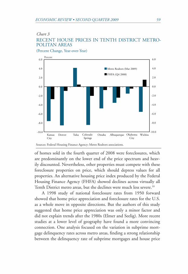
An especially critical factor in explaining foreclosure rates is ap-preciation (or depreciation) in home values. This factor is especially relevant today, when property values have come under immense down-ward pressure. According to regional Realtor associations in the Tenth District, metropolitan areas have seen the median price of homes sold decline as much as 8.5 percent year-over-year (Chart 3). The Realtor association numbers are in some sense artificially low, as 45 percent
Economic REviEw • SEcond quaRtER 2009 59
of homes sold in the fourth quarter of 2008 were foreclosures, which are predominantly on the lower end of the price spectrum and heav-ily discounted. nevertheless, other properties must compete with these foreclosure properties on price, which should depress values for all properties. An alternative housing price index produced by the Federal Housing Finance Agency (FHFA) showed declines across virtually all Tenth District metro areas, but the declines were much less severe.10
A 1998 study of national foreclosure rates from 1950 forward showed that home price appreciation and foreclosure rates for the U.S. as a whole move in opposite directions. But the authors of this study suggested that home price appreciation was only a minor factor and did not explain trends after the 1980s (Elmer and Seelig). More recent studies at a lower level of geography have found a more convincing connection. One analysis focused on the variation in subprime mort-gage delinquency rates across metro areas, finding a strong relationship between the delinquency rate of subprime mortgages and house price
chart 3RECEnT HOUSE PRICES In TEnTH DISTRICT METRO-POLITAn AREAS(Percent Change, year-over-year)
Sources: Federal Housing Finance Agency; Metro Realtors associations.
-10.0
-8.0
-6.0
-4.0
-2.0
0.0
2.0
4.0
6.0
-10.0
-8.0
-6.0
-4.0
-2.0
0.0
2.0
4.0
6.0
KansasCity
Denver Tulsa Colorado Springs
Omaha Albuquerque OkahomaCity
Wichita
Metro Realtors (Mar 2009)
FHFA (Q4 2008)
Percent
60 FeDeRal ReSeRve BanK oF KanSaS CiTy
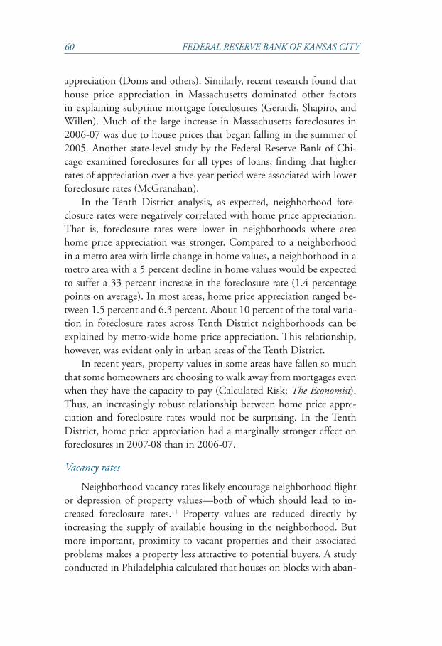
appreciation (Doms and others). Similarly, recent research found that house price appreciation in Massachusetts dominated other factors in explaining subprime mortgage foreclosures (Gerardi, Shapiro, and Willen). Much of the large increase in Massachusetts foreclosures in 2006-07 was due to house prices that began falling in the summer of 2005. Another state-level study by the Federal Reserve Bank of Chi-cago examined foreclosures for all types of loans, finding that higher rates of appreciation over a five-year period were associated with lower foreclosure rates (McGranahan).
In the Tenth District analysis, as expected, neighborhood fore-closure rates were negatively correlated with home price appreciation. That is, foreclosure rates were lower in neighborhoods where area home price appreciation was stronger. Compared to a neighborhood in a metro area with little change in home values, a neighborhood in a metro area with a 5 percent decline in home values would be expected to suffer a 33 percent increase in the foreclosure rate (1.4 percentage points on average). In most areas, home price appreciation ranged be-tween 1.5 percent and 6.3 percent. About 10 percent of the total varia-tion in foreclosure rates across Tenth District neighborhoods can be explained by metro-wide home price appreciation. This relationship, however, was evident only in urban areas of the Tenth District.
In recent years, property values in some areas have fallen so much that some homeowners are choosing to walk away from mortgages even when they have the capacity to pay (Calculated Risk; The economist). Thus, an increasingly robust relationship between home price appre-ciation and foreclosure rates would not be surprising. In the Tenth District, home price appreciation had a marginally stronger effect on foreclosures in 2007-08 than in 2006-07.
vacancy rates
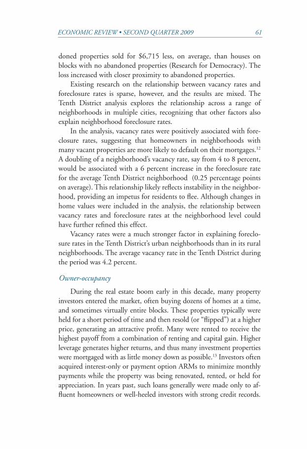
neighborhood vacancy rates likely encourage neighborhood flight or depression of property values—both of which should lead to in-creased foreclosure rates.11 Property values are reduced directly by increasing the supply of available housing in the neighborhood. But more important, proximity to vacant properties and their associated problems makes a property less attractive to potential buyers. A study conducted in Philadelphia calculated that houses on blocks with aban-
Economic REviEw • SEcond quaRtER 2009 61
doned properties sold for $6,715 less, on average, than houses on blocks with no abandoned properties (Research for Democracy). The loss increased with closer proximity to abandoned properties.
Existing research on the relationship between vacancy rates and foreclosure rates is sparse, however, and the results are mixed. The Tenth District analysis explores the relationship across a range of neighborhoods in multiple cities, recognizing that other factors also explain neighborhood foreclosure rates.
In the analysis, vacancy rates were positively associated with fore-closure rates, suggesting that homeowners in neighborhoods with many vacant properties are more likely to default on their mortgages.12 A doubling of a neighborhood’s vacancy rate, say from 4 to 8 percent, would be associated with a 6 percent increase in the foreclosure rate for the average Tenth District neighborhood (0.25 percentage points on average). This relationship likely reflects instability in the neighbor-hood, providing an impetus for residents to flee. Although changes in home values were included in the analysis, the relationship between vacancy rates and foreclosure rates at the neighborhood level could have further refined this effect.
Vacancy rates were a much stronger factor in explaining foreclo-sure rates in the Tenth District’s urban neighborhoods than in its rural neighborhoods. The average vacancy rate in the Tenth District during the period was 4.2 percent.
owner-occupancy
During the real estate boom early in this decade, many property investors entered the market, often buying dozens of homes at a time, and sometimes virtually entire blocks. These properties typically were held for a short period of time and then resold (or “flipped”) at a higher price, generating an attractive profit. Many were rented to receive the highest payoff from a combination of renting and capital gain. Higher leverage generates higher returns, and thus many investment properties were mortgaged with as little money down as possible.13 Investors often acquired interest-only or payment option ARMs to minimize monthly payments while the property was being renovated, rented, or held for appreciation. In years past, such loans generally were made only to af-fluent homeowners or well-heeled investors with strong credit records.
62 FeDeRal ReSeRve BanK oF KanSaS CiTy
More recently, however, underwriting standards were weakened signifi-cantly.
As property values declined, investors often found themselves with properties that could not be sold for sums sufficient to pay off the mortgages, much less to make a profit. According to research by the Mortgage Bankers Association, investors are among the first to default if they see that home prices are falling and there is little chance of re-couping their money (Brinkmann). Some investors have lost numerous properties to foreclosure at one time.
The analysis of foreclosure rates in the Tenth District relies on owner-occupancy rates as an inverse measure of investor-owned properties. The reasoning is that Census-based owner-occupancy statistics can account for properties owned by investors but fraudulently recorded as owner-oc-cupied in mortgage applications, which would underestimate the share of properties in a neighborhood that are investor-owned. Underwriting standards tend to be more lax for mortgages on owner-occupied dwell-ings, so investors could benefit substantially from falsely reporting that they would live in the properties being mortgaged. Such mortgage fraud has been rampant in this decade and continues to increase, even as the real estate market has significantly deteriorated (James, Butts, and Dona-hue). Missouri and Colorado were the ninth- and tenth ranked states for mortgage fraud among 2004-08 originations. Many of the top states for mortgage fraud, including Rhode Island, Florida, Illinois, and Michigan, also have some of the highest foreclosure rates.
About 30 percent of all foreclosures nationally are investor-owned properties.14 In the Tenth District, mortgage applications in 2008 showed that roughly 27 percent of foreclosures were investor-owned properties. Across Tenth District states, the investor share of foreclosures ranged from 14 percent in Wyoming to 49 percent in new Mexico. Of course, to the extent that mortgage fraud is prevalent, this number underestimates the degree of investor penetration in Tenth District neighborhoods. The av-erage owner-occupancy rate in the district is 59 percent.15
While investors clearly are susceptible to default and foreclosure in the face of declining property values, the role of investor-owned prop-erties in explaining foreclosure rates is not altogether clear from a con-ceptual perspective. On one hand, the prototypical investor likely has higher, more diversified net worth than most owner-occupants and is
Economic REviEw • SEcond quaRtER 2009 63
therefore better positioned to suffer through losses. On the other hand, foreclosure often leaves owner-occupants without their valued homes, giving them more of an incentive to stay and find solutions to their mortgage problems.
The Tenth District analysis revealed that foreclosure rates in neigh-borhoods tend to be higher when owner-occupancy rates are higher. In other words, larger shares of investor-owned property surprisingly lead to lower foreclosure rates. But the magnitude of the effect is small. Specifically, a five-percentage-point rise in an owner-occupancy rate is associated with a 0.1-percentage-point rise in the foreclosure rate, a negligible effect. This result suggests that the effect of the typically larger, more diversified portfolios of assets of investors roughly cancels out the often risky nature of investor mortgages.
IV. LOCAL ECONOMIC CONDITIONS
The local economy is an important factor in rising foreclosure rates, both in higher-income neighborhoods and in neighborhoods overall. This section explores the roles of unemployment and self-employment in neighborhood foreclosure rates.
unemployment
Loss of a job or income is one of the most common triggers for mortgage default. A late 1980s study of a large mortgage lender found that 24 percent of seriously delinquent borrowers cited “general finan-cial problems” as the cause of their delinquency, and 21 percent cited job loss specifically (Gardner and Mills).
A cursory look at foreclosure numbers across the nation over the last few years reveals an important role for local economic conditions in determining local foreclosure rates. The Gulf states of Mississippi and Louisiana suffered very high delinquency and foreclosure rates in the aftermath of Hurricanes Katrina and Rita. Likewise, “rustbelt states” like Ohio, Michigan, and Indiana, which have suffered the brunt of the downward trend in manufacturing employment, have maintained some of the highest foreclosure rates over the last few years, at least until recently.16 A review of recent unemployment rates across Tenth District neighborhoods shows a clear relationship between economic conditions and foreclosure rates (Chart 4).
64 FeDeRal ReSeRve BanK oF KanSaS CiTy
Existing research at the national level suggests a weak relationship “at best” between unemployment rates and foreclosure rates over time (Elmer and Seelig). But studies that focus on the state level and zip-code level suggest there is such a relationship (McGranahan; Mian and Sufi). The Tenth District analysis confirms the relationship. Every one- percentage-point rise in the unemployment rate is associated with a 7 percent increase, on average, in the neighborhood foreclosure rate (0.3 percentage points on average).
Self-employment
An additional factor in the Tenth District analysis accounts for dif-ferences in rates of self-employment. Self-employed people tend to have larger incomes than wage and salary workers (Fairlie). At the same time, their incomes generally are more volatile (Jensen and Shore). Given the volatility of income and the recent sharp downturn in economic activ-
Chart 4UnEMPLOyMEnT AnD FORECLOSURE RATES,TEnTH DISTRICT nEIGHBORHOODS
Sources: U.S. Bureau of Labor Statistics; RealtyTrac.
0
5
10
15
20
25
30
0% 2% 4% 6% 8% 10% 12%
Unemployment Rate
Fore
clos
ure
Rat
e
0
5
10
15
20
25
30
Trend line
Percent
Economic REviEw • SEcond quaRtER 2009 65
ity, the self-employed would be more likely to face insufficient funds to make mortgage payments than wage and salary workers, for any given level of income.
Further, the self-employed are more likely to be offered Alt-A and other nontraditional products, like option-ARMs, than wage and salary workers.17 These borrowers often do not qualify for prime loans because their incomes can be hard to document and can be volatile over time.
Two recent surveys by the national Association for the Self-Em-ployed showed the vulnerability of the self-employed. A March 2009 survey showed that 40 percent of participants were concerned about the affordability of their home mortgages due to their type of mortgage. An October 2008 survey showed that 73 percent of survey participants were concerned about the recent downturn in the economy.
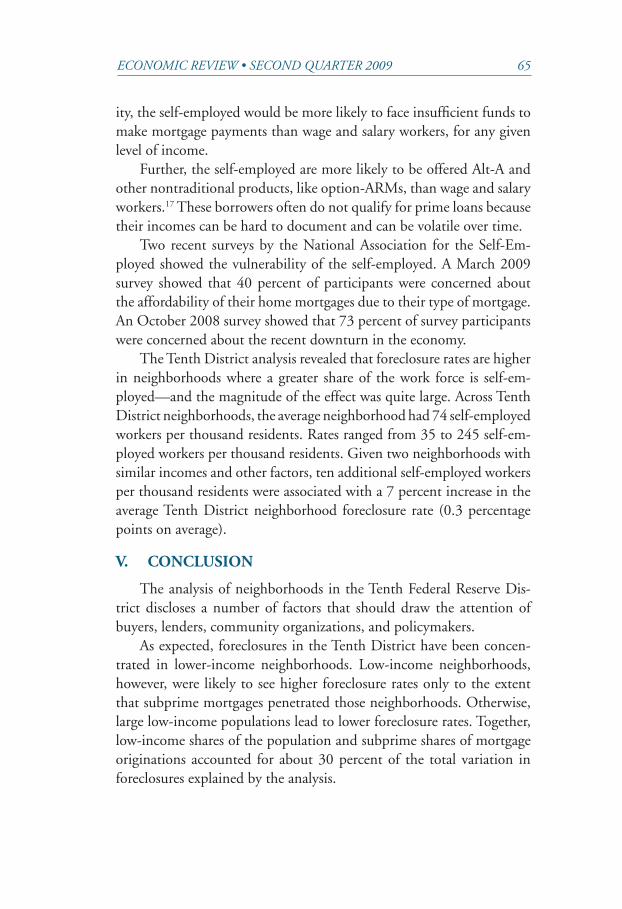
The Tenth District analysis revealed that foreclosure rates are higher in neighborhoods where a greater share of the work force is self-em-ployed—and the magnitude of the effect was quite large. Across Tenth District neighborhoods, the average neighborhood had 74 self-employed workers per thousand residents. Rates ranged from 35 to 245 self-em-ployed workers per thousand residents. Given two neighborhoods with similar incomes and other factors, ten additional self-employed workers per thousand residents were associated with a 7 percent increase in the average Tenth District neighborhood foreclosure rate (0.3 percentage points on average).
V. CONCLUSION
The analysis of neighborhoods in the Tenth Federal Reserve Dis-trict discloses a number of factors that should draw the attention of buyers, lenders, community organizations, and policymakers.
As expected, foreclosures in the Tenth District have been concen-trated in lower-income neighborhoods. Low-income neighborhoods, however, were likely to see higher foreclosure rates only to the extent that subprime mortgages penetrated those neighborhoods. Otherwise, large low-income populations lead to lower foreclosure rates. Together, low-income shares of the population and subprime shares of mortgage originations accounted for about 30 percent of the total variation in foreclosures explained by the analysis.
66 FeDeRal ReSeRve BanK oF KanSaS CiTy
During the current recession, the foreclosure crisis has crept from low-income neighborhoods in the Tenth District into higher-income neighborhoods. Two factors help explain variations in foreclosure rates across these neighborhoods: residential real estate market conditions and local economic conditions.
Real estate market conditions are perhaps the most important fac-tor. Lower price appreciation was associated with higher foreclosure rates. The reasoning is that, in the face of declining property values, ho-meowners having difficulty making mortgage payments may be unable to sell their homes for an amount sufficient to cover their mortgages. Further, if home equity becomes sufficiently negative, homeowners may choose to walk away from their mortgage obligations. Home value appreciation accounted for about 10 percent of the total variation in foreclosures explained by the analysis.
Somewhat unexpected was that higher owner-occupancy rates, or lower shares of investor-owned property, were associated with higher foreclosure rates. A likely factor contributing to this finding is that investors tend to have larger, more diversified financial assets, which makes them better positioned to weather losses. Higher vacancy rates, which diminish neighborhood quality, were also shown to lead to high-er neighborhood foreclosure rates.
Local economic conditions, specifically higher rates of unemploy-ment and self-employment, were also associated with higher foreclosure rates. The magnitude of the unemployment rate effect was quite large: a three-percentage-point difference in the unemployment rate was associ-ated with a 21 percent difference in the foreclosure rate (one percentage point on average). That higher rates of self-employment income were associated with higher foreclosure rates likely reflects the relative volatil-ity of self-employment income, especially during economic recessions. Local economic conditions, though significant, had a much smaller impact on neighborhood foreclosure rates than did income, subprime mortgage penetration, and property appreciation.
Early in the crisis, foreclosures were heavily concentrated in low-income neighborhoods. While low-income neighborhoods continue to suffer from high foreclosure rates, the problem is increasingly seeping into higher-income neighborhoods. This article suggests that buyers, lenders, community organizations, and policymakers should look to
Economic REviEw • SEcond quaRtER 2009 67
neighborhood property conditions and economic conditions to uncover likely future hotspots. Such an analysis would help community orga-nizations and policymakers to best target future preventative resources and buyers and lenders to appropriately gauge risk.
68 FeDeRal ReSeRve BanK oF KanSaS CiTy
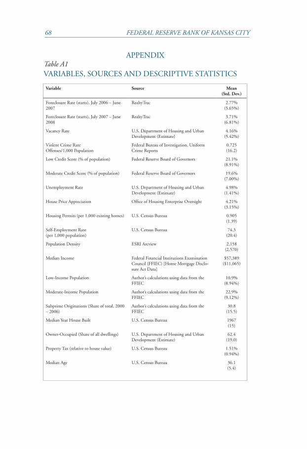
Variable Source Mean(Std. Dev.)
Foreclosure Rate (starts), July 2006 – June 2007
RealtyTrac 2.77%(5.65%)
Foreclosure Rate (starts), July 2007 – June 2008
RealtyTrac 3.71%(6.81%)
Vacancy Rate U.S. Department of Housing and Urban Development (Estimate)
4.16%(5.42%)
Violent Crime RateOffenses/1,000 Population
Federal Bureau of Investigation, UniformCrime Reports
0.725(16.2)
Low Credit Score (% of population) Federal Reserve Board of Governors 21.1% (8.91%)
Moderate Credit Score (% of population) Federal Reserve Board of Governors 19.6% (7.00%)
Unemployment Rate U.S. Department of Housing and Urban Development (Estimate)
4.98% (1.41%)
House Price Appreciation Office of Housing Enterprise Oversight 4.21% (3.15%)
Housing Permits (per 1,000 existing homes) U.S. Census Bureau 0.905 (1.39)
Self-Employment Rate (per 1,000 population)
U.S. Census Bureau 74.3 (20.4)
Population Density ESRI Arcview 2,158 (2,570)
Median Income Federal Financial Institutions Examination Council (FFIEC) [Home Mortgage Disclo-sure Act Data]
$57,389 ($11,065)
Low-Income Population Author’s calculations using data from the FFIEC
10.9% (8.94%)
Moderate-Income Population Author’s calculations using data from the FFIEC
22.9% (9.12%)
Subprime Originations (Share of total, 2000 – 2006)
Author’s calculations using data from the FFIEC
30.8 (15.5)
Median year House Built U.S. Census Bureau 1967 (15)
Owner-Occupied (Share of all dwellings) U.S. Department of Housing and Urban Development (Estimate)
62.4 (19.0)
Property Tax (relative to house value) U.S. Census Bureau 1.51% (0.94%)
Median Age U.S. Census Bureau 36.1 (5.4)
APPEnDIxTable a1VARIABLES, SOURCES AnD DESCRIPTIVE STATISTICS
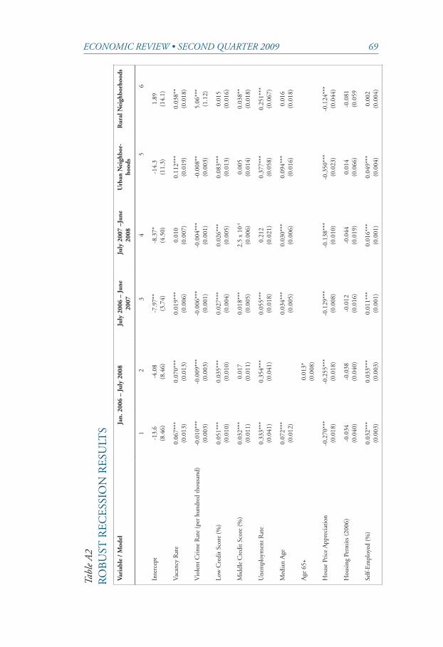
Economic REviEw • SEcond quaRtER 2009 69
tabl
e a
2R
OB
UST
RE
CE
SSIO
n R
ESU
LTS
Vari
able
/ M
odel
J
an. 2
006
– Ju
ly 2
008
July
200
6 –
June
2007
Ju
ly 2
007
–Jun
e 20
08U
rban
Nei
ghbo
r-ho
ods
Rur
al N
eigh
borh
oods
12
34
56
Inte
rcep
t-1
3.6
(8.4
6)-4
.08
(8.4
6)-7
.97*
*(3
.74)
-8.3
7*(4
.50)
-14.
3(1
1.3)
1.89
(14.
1)
Vac
ancy
Rat
e0.
067*
**(0
.013
)0.
070*
**(0
.013
)0.
019*
**(0
.006
)0.
010
(0.0
07)
0.11
2***
(0.0
19)
0.03
8**
(0.0
18)
Vio
lent
Cri
me
Rat
e (p
er h
undr
ed th
ousa
nd)
-0.0
10**
*(0
.003
)-0
.009
***
(0.0
03)
-0.0
06**
*(0
.001
)-0
.004
***
(0.0
01)
-0.0
08**
(0.0
03)
5.06
***
(1.1
2)
Low
Cre
dit S
core
(%
)0.
051*
**(0
.010
)0.
035*
**(0
.010
)0.
027*
**(0
.004
)0.
026*
**(0
.005
)0.
083*
**(0
.013
)0.
015
(0.0
16)
Mid
dle
Cre
dit S
core
(%
)0.
032*
**(0
.011
)0.
017
(0.0
11)
0.01
8***
(0.0
05)
2.5
x 10
-4
(0.0
06)
0.00
5(0
.014
)0.
038*
*(0
.018
)
Une
mpl
oym
ent R
ate
0.33
3***
(0.0
41)
0.35
4***
(0.0
41)
0.05
5***
(0.0
18)
0.21
2(0
.021
)0.
377*
**(0
.058
)0.
251*
**(0
.067
)
Med
ian
Age
0.07
2***
(0.0
12)
0.03
4***
(0.0
05)
0.03
0***
(0.0
06)
0.09
4***
(0.0
16)
0.01
6(0
.018
)
Age
65+
0.01
3*(0
.008
)
Hou
se P
rice
App
reci
atio
n-0
.270
***
(0.0
18)
-0.2
55**
*(0
.018
)-0
.129
***
(0.0
08)
-0.1
38**
*(0
.010
)-0
.350
***
(0.0
23)
-0.1
24**
*(0
.044
)
Hou
sing
Per
mit
s (2
006)
-0.0
34(0
.040
)-0
.038
(0.0
40)
-0.0
12(0
.016
)-0
.044
(0.0
19)
0.01
4(0
.066
)-0
.081
(0.0
59
Self-
Em
ploy
ed (
%)
0.03
2***
(0.0
03)
0.03
3***
(0.0
03)
0.01
1***
(0.0
01)
0.01
6***
(0.0
01)
0.04
9***
(0.0
04)
0.00
2(0
.004
)
70 FeDeRal ReSeRve BanK oF KanSaS CiTy
Vari
able
/ M
odel
Jan.
200
6 –
July
200
8Ju
ly 2
006
– Ju
ne20
07Ju
ly 2
007
–Jun
e 20
08U
rban
Nei
ghbo
r-ho
ods
Rur
al N
eigh
borh
oods
Popu
lati
on D
ensi
ty2.
5 x
10-4**
*(≈
0)
2.4
x 10
-4**
*(≈
0)
1.8
x 10
-4**
*(≈
0)
1.8
x 10
-4**
*(≈
0)
2.2x
10-4
***
(≈ 0
)<
8.1
x 10
-4**
(≈ 0
)
Low
-Inc
ome
Popu
lati
on (
%)
-0.1
12**
*(0
.023
)-0
.102
***
(0.0
23)
-0.0
24**
(0.0
10)
-0.0
69**
*(0
.012
)-0
.113
***
(0.0
31)
-0.1
57**
*(0
.036
)
Mod
erat
e-In
com
e Po
pula
tion
(%
)0.
033*
*(0
.015
)0.
026*
(0.0
15)
-0.0
25**
*(0
.007
)0.
018*
*(0
.008
)0.
021
(0.0
20)
0.05
7**
(0.0
24)
Subp
rim
e O
rigi
nati
ons
(%, 2
000
– 20
06)
0.02
3*(0
.012
)0.
028*
*(0
.012
)-0
.041
***
(0.0
05)
-0.0
06(0
.006
)-0
.014
(0.0
18)
-0.0
29(0
.018
)
Subp
rim
e x
Low
Inc
ome
0.00
2***
(< 5
.0 x
10-4
)0.
002*
**(<
5.0
x 1
0-4)
-3.4
x 1
0-4*
(< 3
.0 x
10-4
)0.
002*
**(<
3.0
x 1
0-4)
3.4
x 10
-4
(< 7
.0 x
10-4
)0.
006*
**(<
7.0
x 1
0-4)
Subp
rim
e x
Mod
erat
e In
com
e8.
8 x
10-4**
(< 5
.0 x
10-4
)8.
4 x
10-4**
(< 5
.0 x
10-4
)0.
003*
**(<
3.0
x 1
0-4)
7.1
x 10
-4**
*(<
3.0
x 1
0-4)
0.00
3***
(< 6
.0 x
10-4
)-0
.001
(< 7
.0 x
10-4
)
Med
ian
year
Hou
se B
uilt
0.00
3(0
.004
)-7
.0 x
10-4
(0.0
04)
0.00
3(0
.002
)0.
003
(0.0
02)
0.00
2(0
.006
)-0
.002
(0.0
07)
Ow
ner
Occ
upie
d (%
)0.
013*
**(0
.003
)0.
016*
**(0
.003
)0.
006*
**(0
.001
)0.
008*
**(0
.002
)0.
011*
**(0
.004
)0.
005
(0.0
06)
Prop
erty
Tax
0.05
8(0
.076
)0.
034
(0.0
76)
-0.0
66**
(0.0
32)
-0.0
27(0
.040
)0.
064
(0.1
00)
-0.0
72(0
.136
)
Afr
ican
-Am
eric
an-0
.053
***
(0.0
10)
-0.0
50**
*(0
.010
)-0
.033
***
(0.0
04)
-0.0
15**
*(0
.005
)-0
.118
***
(0.0
16)
-0.0
39**
*(0
.012
)
Afr
ican
-Am
eric
an x
Sub
prim
e0.
002*
**(<
3.0
x 1
0-4)
0.00
2***
(< 3
.0 x
10-4
)0.
001*
**(<
2.0
x 1
0-4)
8.2
x 10
-4**
*(<
2.0
x 1
0-4)
0.00
3***
(< 4
.0 x
10-4
)0.
002*
**(<
3.0
x 1
0-4)
Asi
an0.
053*
*(0
.024
)0.
034
(0.0
24)
0.02
7**
(0.0
11)
0.01
0(0
.013
)0.
091*
**(0
.030
)-0
.010
(0.0
50)
nat
ive
Haw
aiia
n or
Oth
er P
acifi
c Is
land
er1.
57**
*(0
.334
)1.
51**
*(0
.335
)0.
064
(0.1
48)
1.33
***
(0.1
81)
1.43
***
(0.4
29)
-0.6
93(0
.628
)
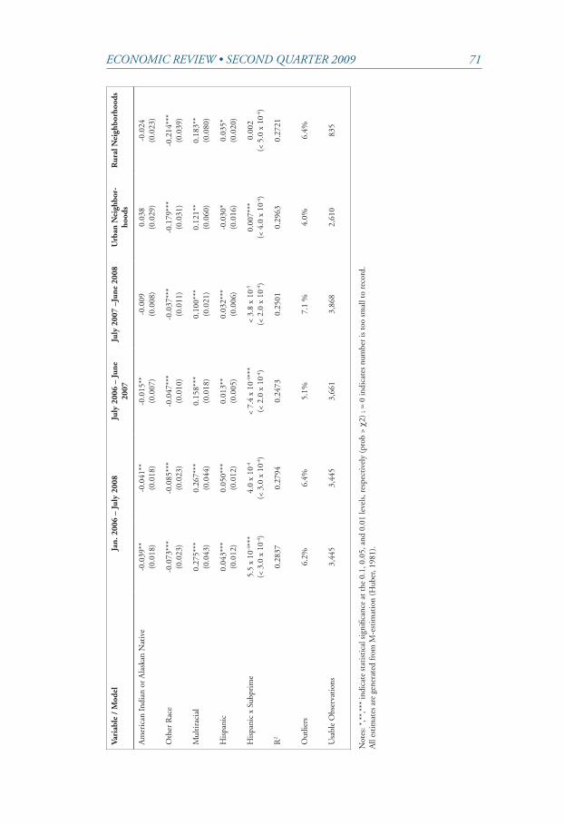
Economic REviEw • SEcond quaRtER 2009 71
Vari
able
/ M
odel
Jan.
200
6 –
July
200
8Ju
ly 2
006
– Ju
ne
2007
July
200
7 –J
une
2008
Urb
an N
eigh
bor-
hood
sR
ural
Nei
ghbo
rhoo
ds
Am
eric
an I
ndia
n or
Ala
skan
nat
ive
-0.0
39**
(0.0
18)
-0.0
41**
(0.0
18)
-0.0
15**
(0.0
07)
-0.0
09(0
.008
)0.
038
(0.0
29)
-0.0
24(0
.023
)
Oth
er R
ace
-0.0
73**
*(0
.023
)-0
.085
***
(0.0
23)
-0.0
47**
*(0
.010
)-0
.037
***
(0.0
11)
-0.1
79**
*(0
.031
)-0
.214
***
(0.0
39)
Mul
tira
cial
0.27
5***
(0.0
43)
0.26
7***
(0.0
44)
0.15
8***
(0.0
18)
0.10
0***
(0.0
21)
0.12
1**
(0.0
60)
0.18
3**
(0.0
80)
His
pani
c0.
043*
**(0
.012
)0.
050*
**(0
.012
)0.
013*
*(0
.005
)0.
032*
**(0
.006
)-0
.030
*(0
.016
)0.
035*
(0.0
20)
His
pani
c x
Subp
rim
e5.
5 x
10-4**
*(<
3.0
x 1
0-4)
4.0
x 10
-4
(< 3
.0 x
10-4
)<
7.4
x 10
-4**
*(<
2.0
x 1
0-4)
< 3.
8 x
10-5
(< 2
.0 x
10-4
)0.
007*
**(<
4.0
x 1
0-4)
0.00
2(<
5.0
x 1
0-4)
R2
0.28
370.
2794
0.24
730.
2501
0.29
630.
2721
Out
liers
6.2%
6.4%
5.1%
7.1
%4.
0%6.
4%
Usa
ble
Obs
erva
tion
s3,
445
3,44
53,
661
3,86
82,
610
835
not
es: *
,**,
***
indi
cate
sta
tist
ical
sig
nific
ance
at t
he 0
.1, 0
.05,
and
0.0
1 le
vels
, res
pect
ivel
y (p
rob
> χ2
) ; ≈
0 in
dica
tes
num
ber
is to
o sm
all t
o re
cord
.A
ll es
tim
ates
are
gen
erat
ed fr
om M
-est
imat
ion
(Hub
er, 1
981)
.
72 FeDeRal ReSeRve BanK oF KanSaS CiTy
EnDnOTES
1In this article, a neighborhood is defined as a Census tract. A Census tract is a small, relatively homogeneous statistical subdivision of a county that numbers between 2,500 and 8,000 in population. Census tracts are designed to reflect the division of counties into neighborhoods.
2There is no universal definition of a subprime mortgage, and thus researchers have used a variety of rubrics to decide which mortgages are subprime and which are not. Options include: (1) loans reported as high-cost in Home Mortgage Dis-closure Act (HMDA) data; (2) home loans originated by lenders who specialize in subprime mortgages, according to a list supplied by the U.S. Department of Housing and Urban Development (HUD); and (3) home loans in securitized pools marketed as subprime. Each method of collecting data on subprime home loans has its advantages and disadvantages (Mayer and Pence). In this study, loans with interest rates of 3 percent or greater above a Treasury security of the same maturity (high-cost loans) were considered subprime. This method was utilized because a larger share of home loans (around 80 percent) is covered in the HMDA data than in the securitized pools marketed as subprime (Avery, Brevoort, and Canner).
3The U.S. foreclosure rate was 3.3 percent in the fourth quarter.4Five neighborhoods in the Tenth District had foreclosure rates above 15
percent, according to foreclosure broker RealtyTrac: three in Pueblo County, CO; one in Adams County, CO; and one in Jackson County, MO.
5Low-income residents are defined as those with income of less than 50 per-cent of the area (state or metropolitan) median income.
6The foreclosure rate is the number of foreclosure starts over the period Janu-ary 2007 — June 2008 relative to the number of mortgages outstanding. Data on foreclosures are estimates from the U.S. Department of Housing and Urban Development (HUD).
7A summary of the analysis is presented in Table 1. A description of data used in the analysis is provided in Appendix Table A1, and full results are provided in Appendix Table A2.
8Because few subprime loans have been originated since mid-2007, the num-ber of subprime loans has dwindled over the last couple of years as loans have cured by default, prepayment, or refinance. In the last two years, the number of subprime loans outstanding has decreased by 11 percent.
9A cash-out refinance is defined here as one where the new mortgage is at least 5 percent higher than the principal on the existing mortgage.
10For more information on housing price indexes, see Rappaport.11Vacancy rate is defined as the number of vacant homes in a neighborhood,
expressed as a percentage of all homes in that neighborhood.
Economic REviEw • SEcond quaRtER 2009 73
12Of course, just as vacancy rates may influence foreclosure rates, the reverse may also be true. While such a relationship is clearly sensible, efforts were taken to ensure that the time period in which vacancy rates were measured preceded the period in which foreclosure rates were measured. An extended analysis that accounts for this possibility in a more sophisticated way confirms the effect of vacancy rates on foreclosure rates.
13Despite late-night infomercials to the contrary, purchasing real estate as investment property with no money down is exceedingly rare.
14This figure is based on properties in the RealtyTrac database where the owner address is different than the property address.
15Data are from the American Housing Survey. Accessed February 10, 2009, at http://www.2010census.biz/hhes/www/housing/ahs/ahs07/tab1a-1.pdf. Roughly 68 percent of all occupied homes are owned by their occupants.
16More recently, states such as Florida and nevada, which experienced espe-cially rapid appreciation earlier in the decade and rampant building, have suffered the highest foreclosure rates.
17Alt-A mortgages are A- rated paper. Generally, the borrower is creditworthy for a prime loan but does not meet some other specified underwriting standard. About 75 percent of Alt-A mortgages were offered to borrowers who did not fully document their income. An option-ARM is an adjustable-rate mortgage where the borrower is allowed to make a minimum payment for a specified period of time. Generally, this payment is well below the fully amortizing payment, so principal builds over time.
74 FeDeRal ReSeRve BanK oF KanSaS CiTy
REFEREnCES
Avery, Robert, Kenneth Brevoort, and Glenn Canner. 2008. “The 2007 HMDA Data,” Federal Reserve Bulletin, vol. 94, December 23, pp. A107-46.
Brinkmann, Jay. 2008. “An Examination of Mortgage Foreclosures, Modifica-tions, Repayment Plans, and Other Loss Mitigation Activities in the Third Quarter of 2007,” Mortgage Bankers Association, January.
Calculated Risk. 2008. “Wachovia: Homeowners Just Walking Away,” January 22, http://www.calculatedriskblog.com.
Chomsisengphet, Souphala, and Anthony Pennington-Cross. 2006. “The Evo-lution of the Subprime Mortgage Market,” Federal Reserve Bank of St. louis, Review, vol. 88, no. 1, pp. 31-56.
Christie, Les. 2008. “Subprime Loans Defaulting Even Before Resets,” Cnn.com, February 20, http://money.cnn.com.
__________. 2007b. “Wow, I Could’ve Had a Prime Mortgage,” Cnn.com, May 30, http://money.cnn.com.
__________. 2007a. “When Bad Loans Get Worse,” Cnn.com, June 21, http://money.cnn.com.
Courchane, Marsha J., Brian J. Surette, and Peter M. Zorn. 2004. “Subprime Borrowers: Mortgage Transitions and Outcomes,” Journal of Real estate Fi-nance and economics, vol. 29, no. 4, pp. 65-92.
Doms, Mark, Fred Furlong, and John Krainer. 2007. “Subprime Mortgage De-linquency Rates,” Federal Reserve Bank of San Francisco Working Paper no. 2007-33.
economist, The. 2008. “Searching for Plan B: As America’s Mortgage Mess Wors-ens, Radical Solutions Are Gaining Appeal,” February 28, http://www.econo-mist.com.
Elmer, Peter J., and Steven A. Seelig. 1998. “The Rising Long-Term Trend of Sin-gle-Family Mortgage Foreclosure Rates,” FDiC Working Paper 98-2, February.
Fairlie, Robert W. 2005. “Self-Employment, Entrepreneurship, and the nLSy79,” Monthly labor Review, vol. 128, no. 2, pp. 40-47.
Gardner, Mona J., and Dixie L. Mills. 1989. “Evaluating the Likelihood of Default on Delinquent Loans,” Financial Management, vol. 18, no. 4, pp. 55-63.
Gerardi, Kristopher, Adam Hale Shapiro, and Paul S. Willen. 2008. “Subprime Outcomes: Risky Mortgages, Homeownership Experiences, and Foreclo-sures,” Federal Reserve Bank of Boston Working Paper 07-15, May.
Huber, Peter S. 1981. Robust Statistics. new york, ny: John Wiley and Sons.James, Denise, Jennifer Butts, and Michelle Donahue. 2009. “Eleventh Periodic
Mortgage Fraud Case Report to the Mortgage Bankers Association,” Mort-gage Asset Research Institute, March.
Jensen, Shane T., and Stephen H. Shore. 2008. “Changes in the Distribution of Income Volatility,” Johns Hopkins University, working paper, June.
Mayer, Chris, and Karen Pence. 2008. “Subprime Mortgages: What, Where, and to Whom?” Federal Reserve Board of Governors, Finance and economic Discus-sion Series, no. 2008-29.
McGranahan, Leslie. 2007. “The Determinants of State Foreclosure Rates: In-vestigating the Case of Indiana,” Federal Reserve Bank of Chicago, Profitwise news and views, December.
Economic REviEw • SEcond quaRtER 2009 75
Mian, Atif, and Amir Sufi. 2008. “The Consequences of Mortgage Credit Ex-pansion: Evidence from the 2007 Mortgage Default Crisis,” national Bureau of economic Research, working paper no. 13936, April.
Mills, Edwin S., and Luan Sende Lubuele. 1994. “Performance of Residential Mortgages in Low- and Moderate-Income neighborhoods,” Journal of Real estate Finance and economics, vol. 9, no. 3, pp. 245-60.
Mortgage Bankers Association. various issues. national Delinquency Survey. national Association for the Self-Employed. 2008. “nASE Member Surveys, Oc-
tober 2008: The Bailout of our Economy,” http://www.nase.com.__________. 2008. “nASE Member Surveys, March 2008: How Is the Hous-
ing Crisis Affecting you?” http://www.nase.com.Rappaport, Jordan. 2007. “A Guide to Aggregate House Price Measures,” Feder-
al Reserve Bank of Kansas City, economic Review, vol. 92, no. 2, pp. 41-71.Research for Democracy. 2001. “Blight Free Philadelphia: A Public-Private Strat-
egy to Create and Enhance neighborhood Value,” Philadelphia, http://www.temple.edu/rfd.
Simon, Ruth. 2009. “The Bailout Plan: U.S. Grasps for a Workable Approach to Foreclosure Crisis,” The Wall Street Journal, February 11, p. A2.