Page 1
i
Characteristics of Noise and Photon Statistics of
Fiber Components in Electro-Optical Systems
By
Cheng Zhao
Submitted in Partial Fulfillment of the
Requirements for the Degree
Doctor of Philosophy
Supervised by
Professor William R. Donaldson
Program of Materials Science
Department of Mechanical Engineering
Arts, Sciences and Engineering
Edmund A. Hajim School of Engineering and Applied Sciences
University of Rochester
Rochester, New York
2012
Page 2
ii
Dedicated to my parents…
Page 3
iii
Biographical Sketch
Cheng Zhao was born in Shanghai, China, in 1979. She attended Shanghai Jiao Tong
University, China, from 1998 to 2005, graduating with a Bachelor of Science degree in
2002 in Materials Science and Engineering, and a Master of Science degree in 2005 in
Materials Science. She came to the University of Rochester in the fall of 2005 and began
graduate studies in the program of Materials Science, the department of Mechanical
Engineering. She received the Master of Science degree in 2007 and continued the
pursuit of the Doctor of Philosophy degree. Under the supervision of Professor William R.
Donaldson, she carried out her doctoral research in the characterization of fiber
components in electro-optical systems. She received a Frank Horton Graduate Fellowship
from the Laboratory for Laser Energetics from 2011 to 2012.
Page 4
iv
Acknowledgement
First and foremost, I would like to express my sincerest gratitude to my advisor,
Professor William R. Donaldson who has supported me throughout my research with
great patience and knowledge. This thesis would not have been possible without his
enlightened guidance.
I feel very fortunate to work with Prof. Donaldson. With his encouragement and support,
I had the opportunities to audit and watch many courses from the Institute of Optics. I
have learned so much from him in fiber optics and electronic testing methods. It is under
his guidance that I began to study and use Matlab for data acquisition and analysis. He
also helped me build my confidence on theoretical work by teaching me step by step how
to apply finite difference method in simulations.
I would like to thank Prof. Roman Sobolewski. It is the experience working with him that
I began to learn optics and to do experiments with optical components. Honestly, the first
time I saw real lasers, lens, polarizers (at that time, I had no idea what it is) and even
optical tables was in his lab. Most of my knowledge on experimental optics came from
the working experience with him and his group members.
I would also like to thank all my friends in lab, Dr. Shuai Wu, Dr. Xia Lisa Li, Dr. Dong
Pan, Dr. Daozhi Wang, Dr. Allen Cross, Dr. Hiroshi Irie and Dr. Jie Zhang. Without their
help, my research work would have been far more difficult than it was. Special thanks to
Page 5
v
Dr. Yijing Fu from Prof. Fauchet‟s group. I got to learn a lot from his wide knowledge in
optics and programming and his personality.
Finally, I would like to thank my parents for their unconditional love, support and
encouragement in my life.
Page 6
vi
Abstract
This thesis presents a comprehensive study of the role of the fiber replicator in electro-
optical systems.
In the all fiber optical diagnostic system for the National Ignition Facility‟s DANTE data
acquisition system running at 1550nm, the 8× fiber replicator was used to increase the
SNR (Signal to Noise Ratio) of single-shot, electrical pulse measurements. In the system,
Mach-Zehnder modulators were used to convert the electrical signals into optical signals.
The fiber replicator was used to create identical copies of the optical signals. A High
SNR was achieved through the averaging of these duplicated signals. Erbium-doped fiber
amplifiers (EDFAs) were built to amplify the optical signals after the fiber replicator.
The EDFAs applied in the DANTEEO system should have high gain, low noise, low
background signals and high pulse-shape fidelity. In this thesis, we discussed the effect of
different configurations and the type of Er-doped fibers on the gain and noise
performance of EDFAs. We also used a simplified model for dynamic gain in EDFAs to
explore the effect of the EDFA on the shape of the amplified pulse. Based on this model,
the calculated pulse-shape distortions were found to be dependent on the EDFA
configuration and the optical gain.
We also investigated the photon statistics with the fiber replicator in a photon
entanglement system. The entangled photons were created through the up-conversion and
down-conversion of a Q-switch laser beam running at 1053nm. The different behavior
Page 7
vii
between entangled photon and non-entangled single photons in the system with the fiber
replicator are discussed.
Page 8
viii
Contributors and Funding Sources
Unless otherwise specified, the author performed all experimental procedure and
simulations presented in this Ph.D. thesis. Other contributions from colleagues and
collaborates are listed below:
The fiber replicators (both 8× replicator in Chapter 3 and 64× replicator in Chapter 6)
were built by Richard Roides at the Laboratory for Laser Energetics.
The NIF DANTEEO system was assembled by Dr. Limin Ji.
The dither suppression system for MZMs was built by Kirk Miller from National
Security Technologies LLC.
This work was supervised by a dissertation committee consisting of Professors William R.
Donaldson (advisor), Roman Sobolewski, and Qiang Lin of the Department of Electrical
and Computer Engineering and Professor John C. Lambropoulos of the Materials Science
Program and the Department of Mechanical Engineering. Graduate study was supported
by a Frank Horton Fellowship from the Laboratory for Laser Energetics. All other work
conducted for the dissertation was completed by the student independently. The work
was supported by the (U.S.) Department of Energy (DOE) Office of Inertial Confinement
Fusion under Cooperative Agreement No.DE-FC52-08NA28302, the University of
Rochester, and the New York State Energy Research and Development Authority.
Page 9
ix
Table of Contents
Biographical Sketch ........................................................................................................... iii
Acknowledgement ............................................................................................................. iv
Abstract .............................................................................................................................. vi
Contributors and Funding Sources................................................................................... viii
Table of Contents ............................................................................................................... ix
List of Tables ................................................................................................................... xiii
List of Figures .................................................................................................................. xiv
List of Symbols ............................................................................................................... xxv
Chapter 1: Introduction ................................................................................................... 1
1.1 Single-shot optical pulse measurement with 256-channel fiber replicator ............... 2
1.2 NIF DANTE system ................................................................................................. 3
1.3 Erbium-doped Fiber Amplifiers (EDFA) in modern telecom industry .................... 5
1.4 EDFAs Applied in the DANTEEO System .............................................................. 7
1.5 Thesis Outline ........................................................................................................... 9
Reference ...................................................................................................................... 11
Chapter 2: General principles on fiber components ..................................................... 14
2.1 Fiber components in electro-optical systems .......................................................... 14
Page 10
x
2.1.1 Fiber Replicator ............................................................................................... 14
2.1.2 Mach-Zehnder Intensity Modulator (MZM) .................................................... 15
2.1.3 Wavelength division multiplexing (WDM) ..................................................... 18
2.2 Erbium-doped fiber amplifier ................................................................................. 19
2.2.1 Spectra of Er3+
dopant in silica fiber and cross sections .................................. 20
2.2.2 Three-level system ........................................................................................... 22
2.2.3 Steady-state gain .............................................................................................. 24
2.2.4 Amplifier noise ................................................................................................ 27
2.2.5 Transient gain................................................................................................... 30
Reference ...................................................................................................................... 35
Chapter 3: Erbium-doped fiber amplifiers (EDFAs) for NIF DANTE system ............ 38
3.1 EO diagnostic system for NIF DANTE (NIF DANTEEO) .................................... 38
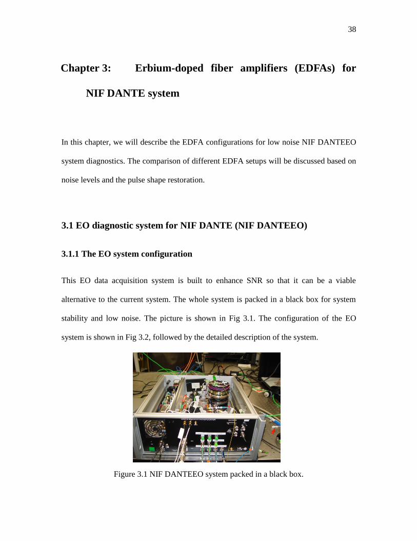
3.1.1 The EO system configuration .......................................................................... 38
3.1.2 System specifications of the components ........................................................ 39
3.2 Characterization of the commercial EDFA............................................................. 46
3.3 Characterization of EDFAs ..................................................................................... 53
3.3.1 EDFAs with L-band Er-doped fiber and multi-stage configuration ................ 53
Page 11
xi
3.3.2 Performance of EDFAs with L-band and/or C-band Er-doped fibers ............. 68
3.3.3 The addition of a holding channel and its effect on EDFA spectrum .............. 84
Reference ...................................................................................................................... 87
Chapter 4: Numerical simulations of transient gains for EDFAs in the DANTEEO
system……… ................................................................................................................... 89
4.1 Simulation method .................................................................................................. 89
4.2 Simulation parameters ............................................................................................ 94
4.3 Simulation results and discussion ......................................................................... 101
4.3.1 Single-stage forward pumping EDFAs .......................................................... 102
4.3.2 Double-stage EDFAs ..................................................................................... 109
4.3.3 Applications of the simulation results in NIF DANTEEO system ................ 118
Reference .................................................................................................................... 123
Chapter 5: General principles on photon entanglements ............................................ 124
5.1 EPR paradox and Entanglement ........................................................................... 124
5.2 Bell-type inequalities ............................................................................................ 126
5.3 Energy-time entanglement .................................................................................... 129
Reference .................................................................................................................... 131
Page 12
xii
Chapter 6: Experimental Setup and Discussion for two photon entanglement .......... 134
6.1 Experimental Setup ............................................................................................... 134
6.1.1 Light source ................................................................................................... 134
6.1.2 Time-bin entanglement system ...................................................................... 136
6.2 Characterization of photon distribution without SPDC ........................................ 140
6.3 Characterization of time-bin entangled photon distribution ................................. 144
Reference .................................................................................................................... 153
Chapter 7: Conclusions and Future Work .................................................................. 154
Page 13
xiii
List of Tables
Table 3.1 Parameters for the DFB laser ............................................................................ 39
Table 3.2 Parameters of the commercial EDFA [1]. ....................................................... 46
Table 3.3 Optical Parameters of the EDFA pumping laser [11]. ...................................... 57
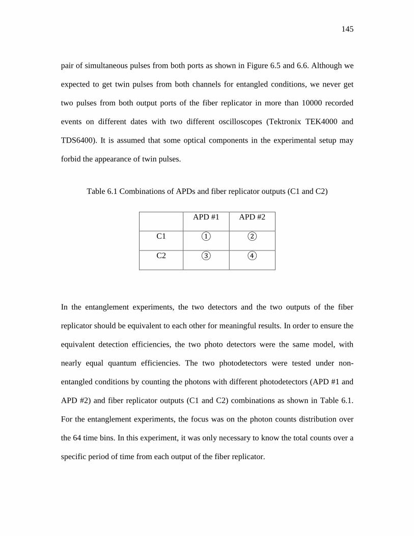
Table 6.1 Combinations of APDs and fiber replicator outputs (C1 and C2) .................. 145
Page 14
xiv
List of Figures
Figure 1.1 Schematic of the single-shot optical pulse measurement system [6]. .............. 3
Figure 1.2 NIF DANTE system illustration (a) and SCD5000s digitizer (b). The parts in
the orange dashed circle are to be replaced with a new EO system. .................................. 4
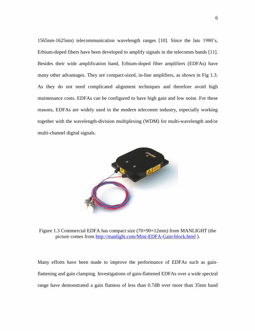
Figure 1.3 Commercial EDFA has compact size (70×90×12mm) from MANLIGHT (the
picture comes from http://manlight.com/Mini-EDFA-Gain-block.html ). ......................... 6
Figure 2.1 Schematic of a 64-pulse fiber replicator with delay-line configuration. ......... 15
Figure 2.2 Schematic of the Mach-Zehnder Modulator (MZM). ..................................... 16
Figure 2.3 Schematic of a MZM operating in linear range. (The transmission vs. voltage
curve is plotted using Vπ= 5 V and Ф= - 0.4π.) ................................................................ 17
Figure 2.4 Energy level of Er3+
dopant in silica fiber [22]. .............................................. 21
Figure 2.5 The three-level simplified system of Er3+
in glass. ......................................... 22
Figure 2.6 Simulation of the signal gain vs. pump power (a) and vs. the fiber length (b).
The signal is at 1550.116nm, pumping wavelength is 980nm, Er-doped fiber length is
10m, the input signal is -30dBm (0.001mW). This simulation was done with the software
“GainMaster” from Fibercore Limited with the single stage forward pumping setup. .... 27
Figure 2.7 Schematic of the experimental setup for the phase sensitive amplifier. Black
and blue lines represent optical and electrical connections, respectively. The inset plots
Page 15
xv
show the input spectra of phase-insensitive and phase-sensitive amplifications,
respectively. BER sensitivity was measured at port A and B by considering PSA as a pre-
or inline amplifier, respectively. CW, continuous wave; NFA, noise-figure analyzer; OSA,
optical spectrum analyzer; PM, phase modulator; PC, polarization controller; PZT,
piezoelectric transducer; PD, photodetector; TDL, tunable delay line; VOA, variable
optical attenuator; PRBS, pseudo-random bit sequence; BER, bit-error ratio; TX,
transmitter [33].................................................................................................................. 29
Figure 2.8 The typical signal pulse shape in the DANTEEO system. The left corner is a
whole train pulses generated by a fiber replicator. ........................................................... 31
Figure 2.9 An example of the transient response. Inset shows the same transient response
over a long time period. Δt expresses the time span for changing the gain by 0.5 dB from
the initial value after changing the input channel number [37]. ....................................... 34
Figure 3.1 NIF DANTEEO system packed in a black box. .............................................. 38
Figure 3.2 The schematic of the EO system for NIF DANTE (a). The thick black arrows
represent electrical signals and the thin black arrows represent optical signals. Schematics
of 4× (b) and 2× (c) replicator used in the DANTE system shown in (a). ....................... 40
Figure 3.3 Schematic of commercial Mach-Zehnder bias controller [1]. ......................... 43
Figure 3.4 Calibration of both MZ modulators. ................................................................ 43
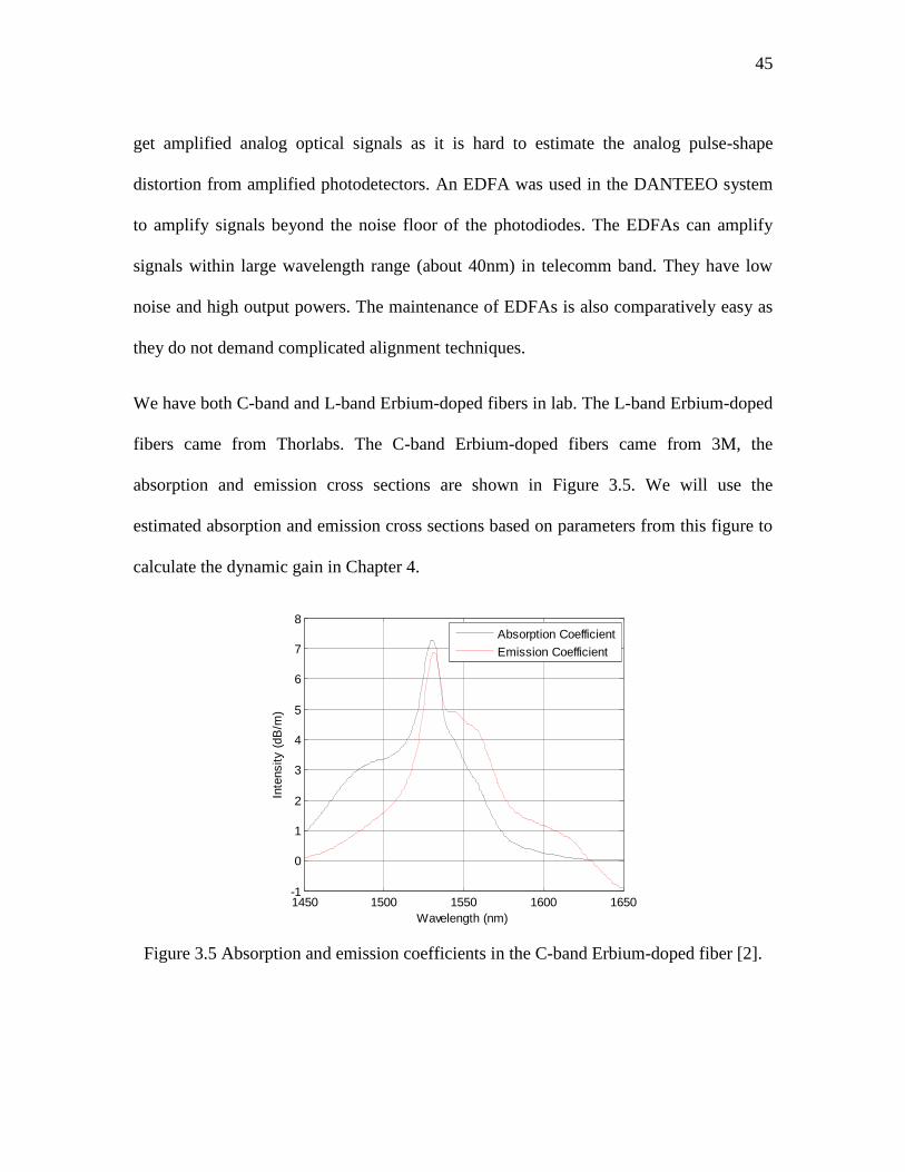
Figure 3.5 Absorption and emission coefficients in the C-band Erbium-doped fiber [2]. 45
Page 16
xvi
Figure 3.6 The pulse trains from 4× output with an amplified photodetector (a) and 8×
output amplified by the commercial EDFA with 90 mA pumping current (b). ............... 47
Figure 3.7 The relationship between the amplitude ratio between 4× output signals and
the EDFA pumping current. Curves come from two different measurements. ................ 48
Figure 3.8 The amplified signals with the pumping current at 190 mA. .......................... 49
Figure 3.9 The pulses realigned and normalized based on the first pulse modulated by
Mach-Zehnder #1 (a). The red curve represents the first pulse, the blue curve represents
the last pulse, and the green curve is the averages of each eight replicas. (b) The
calculated SNR vs. time corresponding to the pulses in (a). ............................................ 50
Figure 3.10 The pulses realigned and normalized based on the first pulse modulated by
Mach-Zehnder #2 (a). The red curve represents the first pulse, the blue curve represents
the last pulse, and the green curve is the averages of each eight replicas. (b) The
calculated SNR vs. time corresponding to the pulses in (a). ............................................ 51
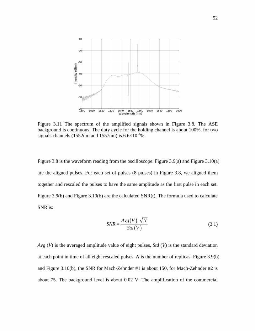
Figure 3.11 The spectrum of the amplified signals shown in Figure 3.8. The ASE
background is continuous. The duty cycle for the holding channel is about 100%, for two
signals channels (1552nm and 1557nm) is 6.6×10⁻³
%. .................................................... 52
Figure 3.12 Two-stage dual forward pumping EDFA experimental setup. ..................... 56
Figure 3.13 Two-stage forward and backward pumping EDFA experimental setup. ...... 57
Figure 3.14 The amplified signals with the configuration shown in Figure 3.12. ............ 58
Page 17
xvii
Figure 3.15 The pulses (from Figure 3.14) realigned and normalized based on the first
pulse modulated by Mach-Zehnder #1 (a). The red curve represents the first pulse, the
blue curve represents the last pulse, and the green curve is the averages of each eight
replicas. (b) The calculated SNR vs. time corresponding to the pulses in (a). ................. 59
Figure 3.16 The pulses (from Figure 3.14) realigned and normalized based on the first
pulse modulated by Mach-Zehnder #2 (a). The red curve represents the first pulse, the
blue curve represents the last pulse, and the green curve is the averages of each eight
replicas. (b) The calculated SNR vs. time corresponding to the pulses in (a). ................. 60
Figure 3.17 The amplified signals with the configuration shown in Figure 3.13. ............ 61
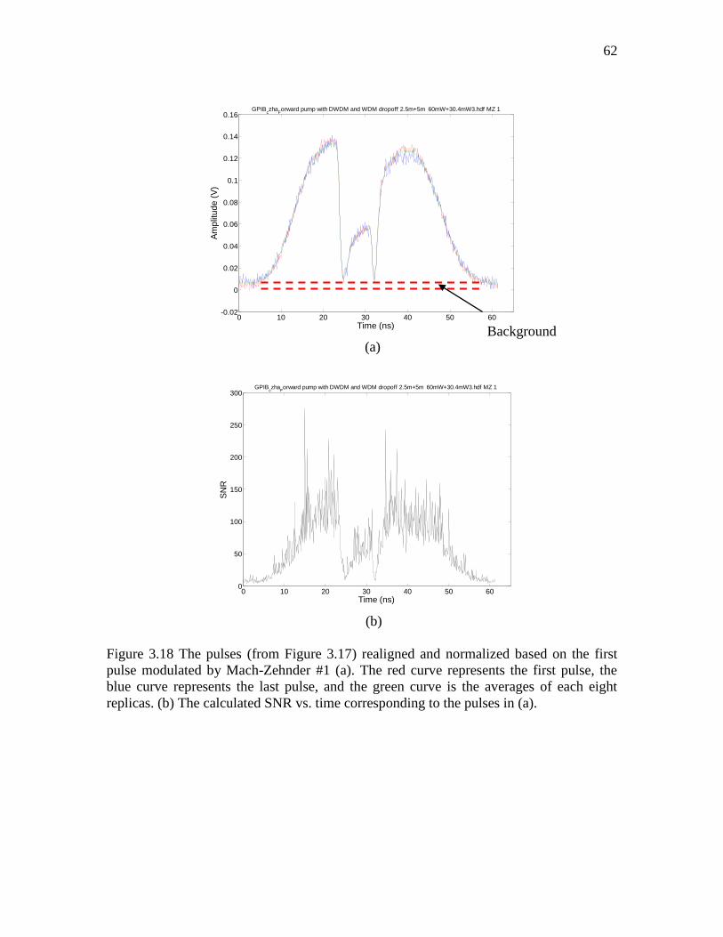
Figure 3.18 The pulses (from Figure 3.17) realigned and normalized based on the first
pulse modulated by Mach-Zehnder #1 (a). The red curve represents the first pulse, the
blue curve represents the last pulse, and the green curve is the averages of each eight
replicas. (b) The calculated SNR vs. time corresponding to the pulses in (a). ................. 62
Figure 3.19 The pulses (from Figure 3.17) realigned and normalized based on the first
pulse modulated by Mach-Zehnder #2 (a). The red curve represents the first pulse, the
blue curve represents the last pulse, and the green curve is the averages of each eight
replicas. (b) The calculated SNR vs. time corresponding to the pulses in (a). ................. 63
Figure 3.20 Comparisons of the SNRs at different signal amplitudes (a) dual forward
pumping scheme, the configuration shown in Figure 3.12 (b) forward and backward
pumping scheme, the configuration shown in Figure 3.13. The dashed blue lines are the
Page 18
xviii
fittings of the SNR vs. Amplitude. The dashed and point green lines in the two figures are
the SNR at the signal amplitude 0.1 V reading from the oscilloscope. ............................ 64
Figure 3.21 Comparisons of pulse shape with the signals amplified by two EDFAs. ...... 66
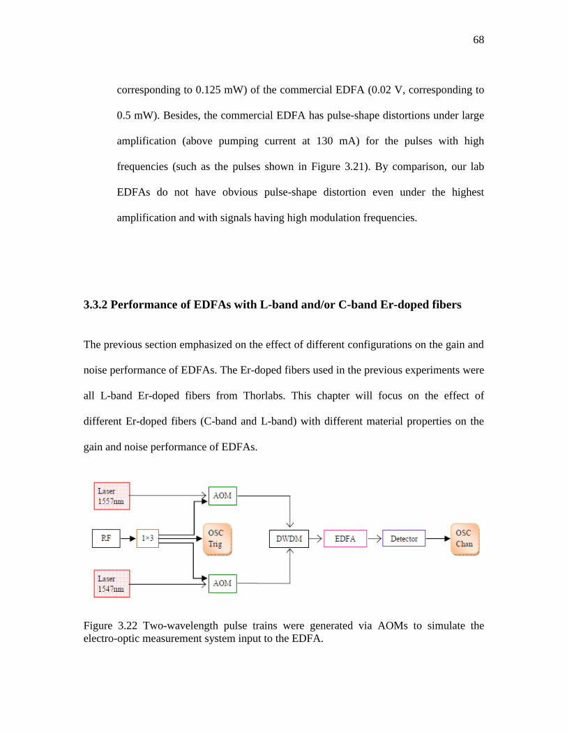
Figure 3.22 Two-wavelength pulse trains were generated via AOMs to simulate the
electro-optic measurement system input to the EDFA. .................................................... 68
Figure 3.23 A single-stage EDFA configuration for testing different types of optical fiber.
........................................................................................................................................... 69
Figure 3.24 Signals from a single-stage EDFA with C-band Er-doped fibers. The typical
waveform read directly from the oscilloscope, the pump power is 25mW at 980nm. ..... 70
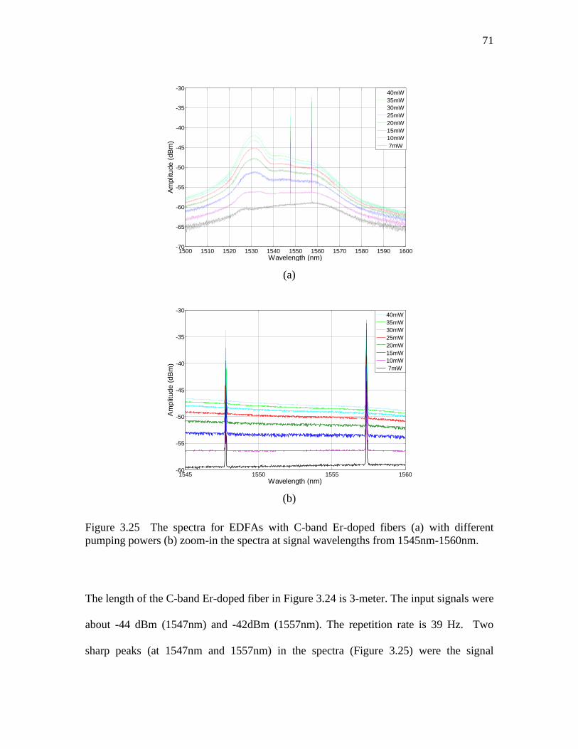
Figure 3.25 The spectra for EDFAs with C-band Er-doped fibers (a) with different
pumping powers (b) zoom-in the spectra at signal wavelengths from 1545nm-1560nm. 71
Figure 3.26 Signals from single-stage EDFA with the L-band Er-doped fiber. (a) The
typical waveform reading from the oscilloscope, pump power is 100mW. (b) The spectra
under different pump powers. The red circle shows the spectral hole burning (SHB). .... 73
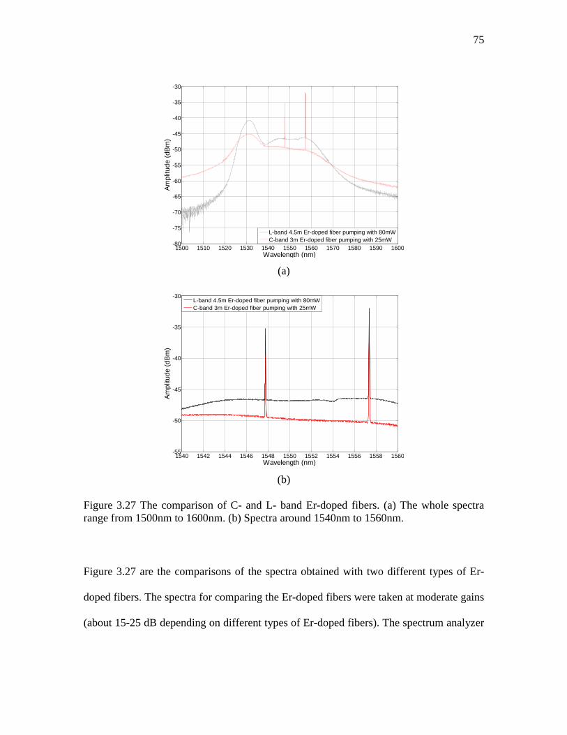
Figure 3.27 The comparison of C- and L- band Er-doped fibers. (a) The whole spectra
range from 1500nm to 1600nm. (b) Spectra around 1540nm to 1560nm. ....................... 75
Figure 3.28 Signals from the single-stage EDFA with C-band + L-band Er-doped fiber. (a)
The typical waveform reading from the oscilloscope, pumping power is 100mW. (b) The
spectra for different pump powers. ................................................................................... 77
Page 19
xix
Figure 3.29 Signals from single-stage EDFA with L-band + C-band Er-doped fibers. (a)
The typical waveform reading from the oscilloscope, pumping power is 100mW. (b) The
spectra with different pumping power. The blue circle illustrates the spectral
characteristic of parasitic oscillations. .............................................................................. 79
Figure 3.30 Free running ASE signals. The left small plot is the corresponding spectral
measurement. .................................................................................................................... 81
Figure 3.31 Comparisons of the EDFA gain spectrum using different Er-doped fibers. . 82
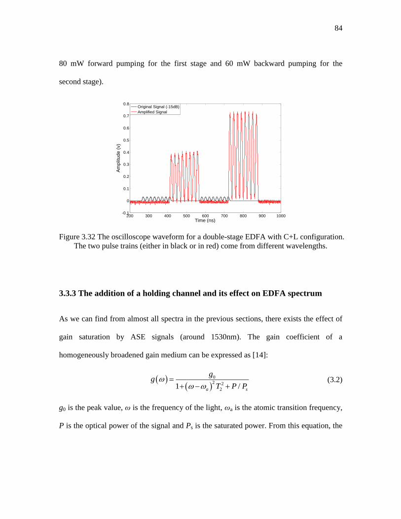
Figure 3.32 The oscilloscope waveform for a double-stage EDFA with C+L configuration.
The two pulse trains (either in black or in red) come from different wavelengths. .......... 84
Figure 3.33 Waveforms of holding and signal channels used in the electro-optic data
acquisition system. ............................................................................................................ 85
Figure 3.34 The gain spectra of the signals as a function of the holding channel power. 86
Figure 4.1 Schematic of the finite difference method in the calculation of the EDFA gain.
........................................................................................................................................... 91
Figure 4.2 The schematic of the finite-difference method applied in the calculation of
transient gain in EDFAs. ................................................................................................... 93
Figure 4.3 Absorption and Emission Coefficients of C- and L-band Erbium-doped fibers
at working wavelengths (a) and pump wavelengths (b). Data comes from [5]. ............... 94
Page 20
xx
Figure 4.4 The calculated boundary conditions. (a) GainMaster‟s result (b) the
comparison of the simulated result with the GainMaster‟s result (c) the EDFA
configuration for the boundary condition calculated with GainMaster shown in (a). ..... 96
Figure 4.5 The relation between inversion level and different fiber parameters. (a)
Inversion level vs. overlap factor for the pump wavelength (b) Inversion level vs. overlap
factor for signal (ASE) wavelengths (c) Inversion level vs. doping concentration,
assuming overlap factors are 0.5 for both the pump and signal wavelengths. .................. 98
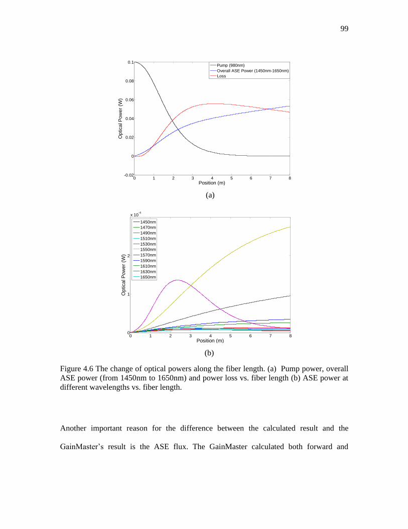
Figure 4.6 The change of optical powers along the fiber length. (a) Pump power, overall
ASE power (from 1450nm to 1650nm) and power loss vs. fiber length (b) ASE power at
different wavelengths vs. fiber length. .............................................................................. 99
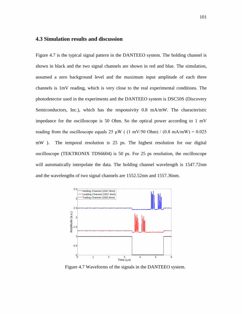
Figure 4.7 Waveforms of the signals in the DANTEEO system. ................................... 101
Figure 4.8 Schematic of the single-stage forward pumping EDFA configuration in
simulations. ..................................................................................................................... 102
Figure 4.9 Waveforms and gain plots with 60mW pump power. The signals from the first
and the second channels are shown in (a) and (c). The differences between the
renormalized signals are shown in (b) and (d), corresponding to (a) and (c). ................ 103
Figure 4.10 Simulated results (a) The derivative of the gain with respect to time vs. time
for three channels. (b) The semi-log plots of gain vs. time for two signal channels. ..... 105
Figure 4.11 The amplitude differences under different pump powers. (a) The maximum
values of amplitude difference vs. pumping power (b) The minimum values of amplitude
Page 21
xxi
difference vs. pumping power. The small plot shows the definition of max and min values
of the amplitude differences............................................................................................ 106
Figure 4.12 Gain and differential gain with different pump powers. (a) 120 mW (b) 180
mW (c) 240 mW (d) 300 mW. ........................................................................................ 108
Figure 4.13 Schematic of the double-stage, forward pumping configuration in simulations.
......................................................................................................................................... 109
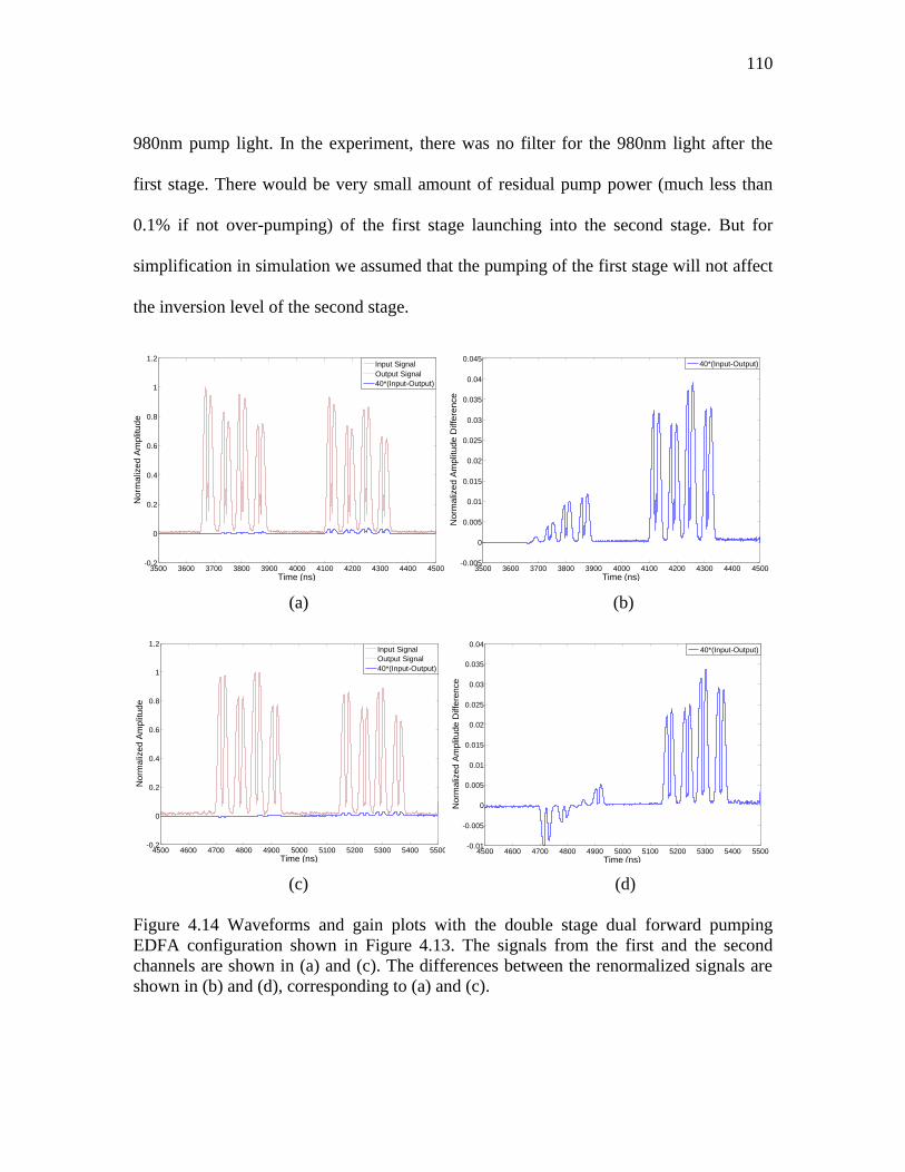
Figure 4.14 Waveforms and gain plots with the double stage dual forward pumping
EDFA configuration shown in Figure 4.13. The signals from the first and the second
channels are shown in (a) and (c). The differences between the renormalized signals are
shown in (b) and (d), corresponding to (a) and (c). ........................................................ 110
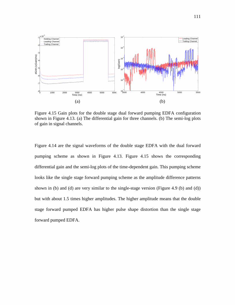
Figure 4.15 Gain plots for the double stage dual forward pumping EDFA configuration
shown in Figure 4.13. (a) The differential gain for three channels. (b) The semi-log plots
of gain in signal channels. ............................................................................................... 111
Figure 4.16 The change of amplitude differences with different pump powers for the
double-stage forward pumping configuration shown in Figure 4.13. (a) The change of
amplitude differences (max and min) with the change of pump powers for the second
stage, the pumping power for the first stage is 60mW. (b) The change of amplitude
differences (max and min) with the change of pumping powers for the first stage, the
pumping power for the second stage is 60mW. .............................................................. 112
Page 22
xxii
Figure 4.17 Configuration of a double stage EDFA with forward and backward pumping
scheme............................................................................................................................. 113
Figure 4.18 Waveforms of the forward and backward pumped double-stage EDFA. The
configuration is shown in Figure 4.17. The signals from the first and the second channels
are shown in (a) and (c). The differences between the renormalized signals are shown in
(b) and (d), corresponding to (a) and (c). ........................................................................ 114
Figure 4.19 Gain plots with the forward and backward pumped double-stage EDFA. The
configuration is shown in Figure 4.17. (a) The differential gain for three channels. (b)
Zoom-in of the time region within red dashed line shown in (a). (c) The semi-log plots of
the gain for signal channels............................................................................................. 115
Figure 4.20 The change of amplitude difference with pump power for the double stage
forward and backward pumping scheme. The configuration is shown in Figure 4.17. (a)
The change of amplitude difference (max and min) with the change of pumping power
for the second stage, the pump power for the first stage is 60mW. (b) The change of
amplitude difference (max and min) with the change of pump power for the first stage,
the pump power for the second stage is 60mW. ............................................................. 116
Figure 4.21 Gain vs. Time. (a) the double-stage with dual forward pumping (b) the
double-stage with forward and backward pumping. ....................................................... 117
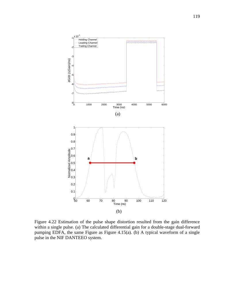
Figure 4.22 Estimation of the pulse shape distortion resulted from the gain difference
within a single pulse. (a) The calculated differential gain for a double-stage dual-forward
Page 23
xxiii
pumping EDFA, the same Figure as Figure 4.15(a). (b) A typical waveform of a single
pulse in the NIF DANTEEO system. .............................................................................. 119
Figure 4.23 Experimental setup for the simulation of the transient gain for a long time
window. (a) The schematic of the experimental setup. (b) The waveform of the input
signal train of the pulses with two wavelengths. The length of the signal train is about 10
μs. .................................................................................................................................... 121
Figure 4.24 Comparison of the experimental and simulation results. ............................ 122
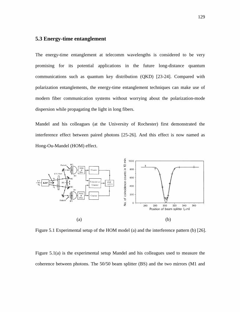
Figure 5.1 Experimental setup of the HOM model (a) and the interference pattern (b) [26].
......................................................................................................................................... 129
Figure 6.1 Block diagram of the multipurpose Nd:YLF laser (a) the Q-switched pulse (b)
[1]. ................................................................................................................................... 135
Figure 6.2 Schematic of the time-bin photon entanglement system. .............................. 137
Figure 6.3 Calibration of the fiber replicator (a) the oscilloscope waveform (b) the
calculated channel width. ................................................................................................ 140
Figure 6.4 Schematic of the system for characterizing the outputs without SPDC. ....... 141
Figure 6.5 Simultaneous signals from both channels of the fiber replicator. The photons
in this measurement are not entangled. ........................................................................... 142
Figure 6.6 Multiple signals from the APDs. The photons in this measurement are not
entangled. ........................................................................................................................ 143
Page 24
xxiv
Figure 6.7 Amplitude Calibration of the 64× fiber replicator with 12.5 ns channel width.
......................................................................................................................................... 144
Figure 6.8 Signals from the oscilloscope (a) single pulse (b) two pulses in one channel (c)
three pulses in one channel. The photons characterized in this figure are possibly
entangled through SPDC................................................................................................. 146
Figure 6.9 Counts per channel for the fiber replicator (a) and (c) are raw data from output
#1 and #2. (b) and (d) are calibrated data. These counts are for photons under entangled
state. ................................................................................................................................ 147
Figure 6.10 Experimental setup for the determination of pulse locations ...................... 149
Figure 6.11 (a) The difference of time-bin locations for two pulses (b) the distribution of
channel for two pulses. ................................................................................................... 150
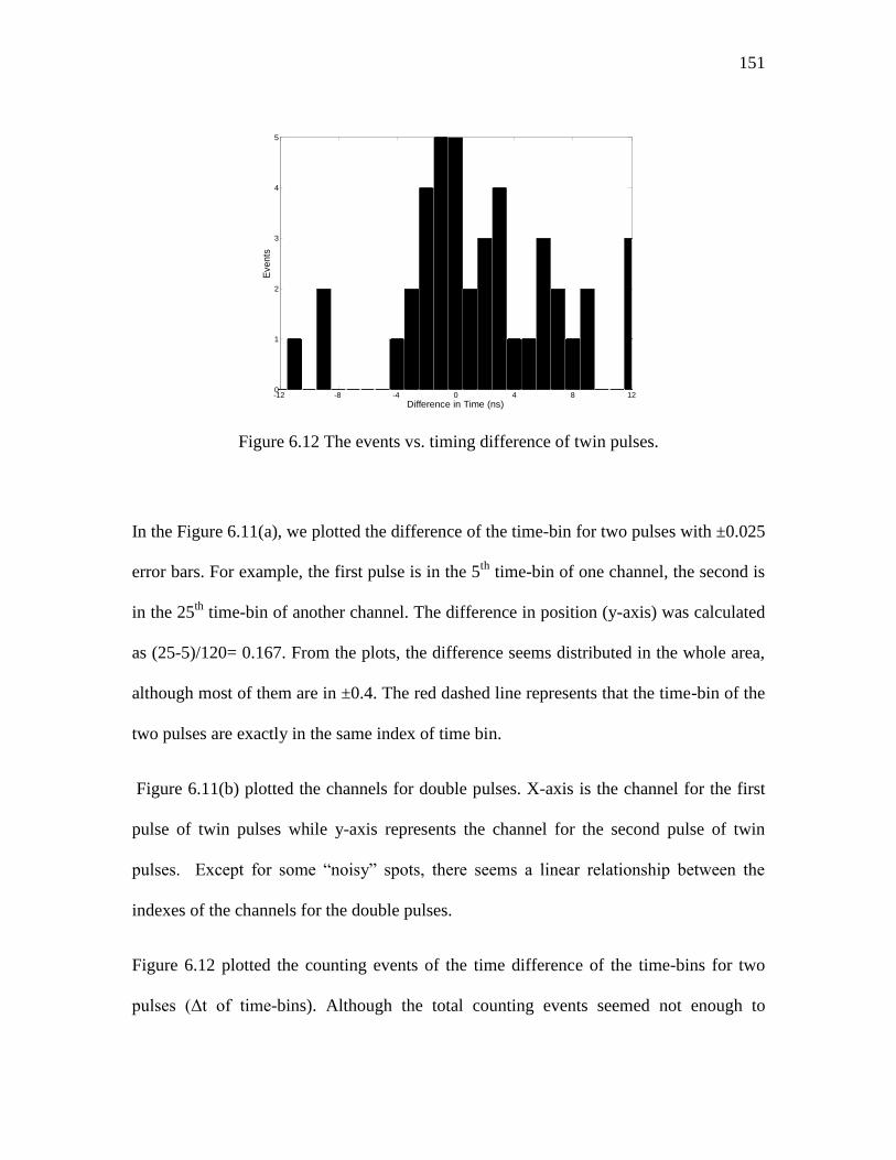
Figure 6.12 The events vs. timing difference of two pulses. .......................................... 151
Page 25
xxv
List of Symbols
SNR signal to noise ratio
EDFA erbium-doped fiber amplifier
EO system electro-optical system
WDM wavelength-division multiplexing
ASE amplified spontaneous emission
SBS stimulated Brillouin scattering
DWDM dense wavelength-division multiplexing
SRS stimulated Raman scattering
V(t) applied electrical signal
Φ(λ) modulator phase bias
Vπ(λ) half-wave voltage of the modulator
d electrode separation
λ optical wavelength
Г(λ) confinement factor
n(λ) index of refraction
r(λ) electrooptic coefficient
Lm electrode length
MZM Mach-Zehnder Modulator
LiNbO3 lithium niobate
CWDM coarse wavelength-division multiplexing
ITU International Telecommunication Union
ESA excited-state absorption
υp signal flux of 1→3 transition
υs signal flux of the 1→2 transition
σp absorption cross section
σs emission cross section
Г32 and Г23 transition possibilities between 3 and 2
Page 26
xxvi
Г21 and Г12 transition possibilities between 1 and 2
N1, N2 and N3 populations of each level
τ2 lifetime of energy level 2
Ip pumping intensity
Aeff effective area
G signal
NF noise figure
Rd responsivity of an ideal photo detector
SASE spectral density of ASE
nsp spontaneous emission factor
γn and αn emission and absorption constants
DFB laser distributed feedback laser
AOM acoustic optical modulator
sat
pP pumping power for saturated gain
Std (V) standard deviations
SHB spectral hole burning
g0 peak value of gain coefficient
ω frequency of the light
ωa atomic transition frequency
u propagation direction
PZT piezoelectric translator
SHG second harmonic generation
SPDC spontaneous parametric down conversion
BBO barium borate (BaB2O4)
IR infrared
Page 27
1
Chapter 1: Introduction
The optically assisted diagnostic systems for electrical signals have been investigated for
many years [1]. Many methods have been explored to increase the limit of the dynamic
range and the speed of oscilloscopes. Optical measurements of electrical signals as fast as
15 ps have been achieved through the use of photoconductive Si switches with
transmission line structures [2]. The linear electro-optic effects (Pockels effect) in LiTO3
and GaAs have also been explored in the electro-optical sampling of ultrafast signals [3-
4]. Electrical signals as fast as 1.1 ps have been detected by a two layer GaAs structure
utilizing the intrinsic Franz-Keldysh effect [5]. However, all these diagnostic methods are
based on repetitive signals and do not work in single-shot range.
In recent years, scientists in the Laboratory for Laser Energetics (LLE) have developed
techniques for an optical diagnostic system for the measurement of single-shot electrical
pulses. There are two such systems currently working in LLE. One system is running at
1053nm with a 256× fiber replicator [6]. Another system is the NIF DANTE system used
in the OMEGA facility at the University of Rochester. The working wavelength is
1550nm.
Page 28
2
1.1 Single-shot optical pulse measurement with 256-channel fiber
replicator
The schematic of the electrical-optical diagnostic system for measuring the pulse shape at
the front end of the OMEGA laser system is shown in Figure 1.1. The CW laser is
running at 1053nm. The optical signal was generated by a fiber Mach-Zehnder electro-
optical modulator fabricated on LiNbO3 [6]. The fiber replicator in this system has a time
window of 12.5 ns. Thus, the pulse width must be less than 12.5 ns to avoid optical
interference between neighboring time windows of the optical replicator. In the system,
there was a two-stage modulator to generate nano-second pulses. Initially, a square
electrical gate pulse was applied to the first modulator to eliminate any light outside of
the temporal duration of the electrical pulse. The second electrical signal drives the
Mach-Zehnder modulator to generate a shaped optical pulse. Because there is a well-
established relationship between the electrical pulse and the optical transmission for the
Mach-Zehnder modulator, it is possible to determine the original input electrical signal of
the Mach-Zehnder modulator by accurately measuring the optical signal out of the Mach-
Zehnder modulator.
Detailed information about how the Mach-Zehnder modulator and the fiber replicator
work will be provided in Chapter 2. The fiber replicator in this system has 256 channels
and 12.5 ns temporal separation, which means the original signal after the amplifier will
have a total of 256 copies with about 12.5 ns pulse separation. As this fiber replicator is a
passive element, the power of each replica would be around 1/256 of the original single
Page 29
3
pulse in terms of the conservation of energy, without considering any other loss. So,
optical amplifiers are needed to amplify the signals for detection in an oscilloscope and to
achieve a high SNR. An Yb-doped fiber amplifier and a regenerative amplifier were used
as optical pre-amplifiers for the 1053-nm system [7-8]. The train of replicated optical
pulses was measured with a photodiode (Discovery Semiconductor DSC30S) and a
digital sampling oscilloscope (Tektronix TDS6154c). By temporally realigning and
amplitude averaging, optical signals with dynamic range as high as 1800:1 can be
measured. An inverse transfer function is applied to the processed optical pulse to trace
back to the input electrical pulse. Since this system was used to measure optical pulses,
the distortion introduced by the pre-amplifiers was irrelevant.
Figure 1.1 Schematic of the single-shot optical pulse measurement system [6].
1.2 NIF DANTE system
The DANTE system is multi-channel soft x-ray spectrometers at the National Ignition
Facility (NIF) at Lawrence Livermore National Laboratory and the OMEGA facility at
Page 30
4
the University of Rochester [9]. They are used to measure radiation drive temperatures
produced in the hohlraums.
(a)
(b)
(b)
Figure 1.2 NIF DANTE system illustration (a) and SCD5000s digitizer (b). The parts in
the orange dashed circle are to be replaced with a new EO system.
Page 31
5
Each DANTE Channel uses two SCD5000 transient digitizers. There are 18 channels per
DANTE and two DANTE instruments on the NIF target chamber for a total of 72
SCD5000s. The SCD5000 transient digitizers have 6 GHz bandwidth, 900:1 dynamic
range and fixed number (1000) of temporal resolution elements. However, these
digitizers are twenty years old and will need to be replaced soon. FTD10000 scopes are
the only direct replacement option, but an FTD10000 costs about $120K per channel.
Considering each DANTE system requires 36 scopes and 2 spares, this will cost a total of
$5 million. Besides, FTD10000 scopes have a life span of 5000 hours while the current
DANTE system will reach 5000 hours in about 2 years. So the new EO system was
designed as a replacement for SCD5000 with higher bandwidth, low noise, lower
maintenance, longer life time, and lower cost. This all-fiber EO system includes the
electro-optical modulators which convert the electrical signal into a modulated optical
signal and makes use of fiber replicators for high SNR, high pulse-shape fidelity optical
diagnostics. A major portion of this thesis is devoted to the improvement of the 1550nm
version of the EO diagnostic system. This is the system that has the most general use.
1.3 Erbium-doped Fiber Amplifiers (EDFA) in modern telecom
industry
The working wavelength of Erbium-doped fibers ranges from 1520nm to 1620nm which
covers most of both the C (conventional band, 1535nm-1565nm) and the L (long band,
Page 32
6
1565nm-1625nm) telecommunication wavelength ranges [10]. Since the late 1980‟s,
Erbium-doped fibers have been developed to amplify signals in the telecomm bands [11].
Besides their wide amplification band, Erbium-doped fiber amplifiers (EDFAs) have
many other advantages. They are compact-sized, in-line amplifiers, as shown in Fig 1.3.
As they do not need complicated alignment techniques and therefore avoid high
maintenance costs. EDFAs can be configured to have high gain and low noise. For these
reasons, EDFAs are widely used in the modern telecomm industry, especially working
together with the wavelength-division multiplexing (WDM) for multi-wavelength and/or
multi-channel digital signals.
Figure 1.3 Commercial EDFA has compact size (70×90×12mm) from MANLIGHT (the
picture comes from http://manlight.com/Mini-EDFA-Gain-block.html ).
Many efforts have been made to improve the performance of EDFAs such as gain-
flattening and gain clamping. Investigations of gain-flattened EDFAs over a wide spectral
range have demonstrated a gain flatness of less than 0.7dB over more than 35nm band
Page 33
7
width by using acousto-optic filters [12]. Other efficient techniques for gain flattening
include high-birefringence fiber loop mirror, different compositions and dual-core
Erbium-doped fiber, equalizing film, fiber Bragg gratings and mechanically induced
microbending fiber gratings [13-19]. EDFAs with WDMs applied in modern optical
network systems have to deal with gain variation problems resulting from adding and
dropping channels or the sudden failure of components. Gain-clamping techniques have
been used to prevent performance degradation, severe service impairment or the
appearance of optical nonlinearities which resulted from a sudden change of gain [20-22].
A variety of solutions have been employed to stabilize the gain, which are mostly based
on using a part of signal, pumping or amplified spontaneous emission (ASE) as the
feedback either via a cavity loop or fiber gratings [23-28]. Stimulated Brillouin
scattering (SBS) also can be used in the feedback to monitor signal gains [29].
After more than twenty years of continuous efforts on improvement, EDFA technologies
have become quite sophisticated.
1.4 EDFAs Applied in the DANTEEO System
Although there are sophisticated commercial EDFAs available, there is still a need to
develop an EDFA for this particular application because the DANTEEO system has
special requirements that are different from standard telecom applications.
Page 34
8
The signals in the DANTEEO system are analog signals, while the signals are
normally digital signals in standard telecom. So the EDFA in the DANTEEO
system should have high signal to noise ratio (estimated to be 200:1) and high
pulse-shape fidelity.
The EDFA in the DANTEEO system is designed to amplify signals at multi-
wavelengths. The DANTEEO system is designed for up to eight wavelengths
(corresponding to ITU-200 and/or DWDM channels) in each channel. So the
EDFA should amplify signals with up to eight different wavelengths. As the
DWDM channels range from 1547.72nm to 1558.98nm, it is quite easy to get
uniform gain for all wavelengths. But the narrow spectral separation will also
cause crosstalk, which will affect signal pulse shape diagnostics. Unlike standard
telecom system, only one wavelength will be in the system at any particular time.
The temporal separation of the wavelengths will affect the gain dynamics of the
EDFA.
For each wavelength, the signal has a train of pulses with temporal separation.
The signal amplitude changes fast (~ns) compared with the transit time in
Erbium-doped fibers. So the EDFA is not working under steady state or quasi
steady-state.
The final signal pulse shape diagnostics will be based on the mathematical
average of those pulses in the time domain. So the gain dynamics, if different for
individual pulses, will also affect the final signal pulse shape.
Page 35
9
The signal pulse train was generated by a fiber replicator. The individual pulses
will have different polarizations as they go through different optical paths within
the fibers. So the polarization related optical fiber components such as the
Faraday isolators are not suitable in this EDFA configuration as they don‟t affect
all pulses evenly.
1.5 Thesis Outline
This thesis consists of two parts, corresponding to the two optical pulse diagnostic
systems currently working in LLE. The major part, Part I, is noise characterization in Er-
doped fiber amplifier (EDFA) used in the single-shot electro-optical diagnostic system
NIF DANTEEO. The target of this experiment is to design an Er-doped fiber amplifier to
replace the commercial EDFA in the current system setup. Low noise, low background
signal, larger amplification and good pulse shape restoration are the major considerations.
The first part of Chapter 2 will introduce the basics of some fiber elements used in the
DANTEEO system. The second part of Chapter 2 covers the fundamental mechanisms of
the gain process, including three-level amplification basics, absorption and emission
cross sections, and amplified spontaneous emission. The experimental setup and the
discussion of the results will be in Chapter 3. The discussion will emphasize on how the
Er-doped fiber length and pump powers affect both the noise and the shape restoration.
The numerical simulation of the EDFA gain dynamics will be in Chapter 4. We will
discuss how the difference in gain dynamics affects pulse shapes.
Page 36
10
Part II is the photon statistics with the fiber replicator in a photon entanglement
system. Originally this section started as an investigation of the noise in fiber
replicators as the signal approached the single photon level. This investigation
expanded into an investigation of the photon entanglement. Chapter 5 will emphasize
the basic idea and the progress of our photon entanglement investigation. The detailed
experimental setup (including the complete up-conversion and down-conversion, and
the alignment process) and the results will be presented in Chapter 6. The different
behavior between an entangled photon and a non-entangled photon in the system with
the fiber replicator will be discussed.
Chapter 7 is dedicated to the conclusions of this thesis and a description of the future
work.
Page 37
11
Reference
1. A. S. Bhushan, P. V. Kelkar, B. Jalali, O. Boyraz, M. Islam, “130-GSa/s Photonic
Analog-to-Digital Converter With Time Stretch Preprocessor”, IEEE Photon. Technol.
Lett., vol. 14, No. 5, 2002.
2. D. H. Auston, “Picosecond optoelectronic switching and gating in silicon”, Appl. Phys.
Lett., vol. 26, pp. 101, 1975
3. J. A. Valdmanis, G. Mourou, and C. W. Gabel, “Picosecond electrooptic sampling
system”, Appl. Phys. Lett., vol. 41, pp. 211, 1982.
4. G. A. Mourou and K. E. Meyer, “Subpicosecond electro‐optic sampling using coplanar
strip strip transmission lines”, Appl. Phys. Lett. vol.45, pp. 492, 1984.
5. J. F. Lampin, L. Desplanque, F. Mollot, “Detection of picosecond electrical pulses
using the intrinsic Franz–Keldysh effect”, Appl. Phys. Lett., vol. 78, pp. 4103, 2001.
6. W. R. Donaldson, J. R. Marciante, R. G. Roides “An Optical Replicator for Single-
Shot Measurements at 10 GHz With a Dynamic Range of 1800:1”, IEEE Journal of
Quantum Electronics, vol. 46, No.2, 2010.
7. J. R. Marciante, J. D. Zuegel, “High-gain, polarization-preserving, Yb-doped fiber
amplifier for low-duty-cycle pulse amplification”, Appl. Opt., vol. 45, pp. 6798, 2006.
8. A. V. Okishev and J. D. Zuegel, “Highly stable, all-solid-state ND:YLF regenerative
amplifier”, Appl. Opt., vol. 43, pp. 6180, 2004.
9. Donald Pellinen, Matthew Griffin, National Security Technologies, LLC (NSTec).
Livermore Operations (LO), DOE/NV/25946-086.
10. Ramaswami, Rajiv “Optical Fiber Communication: From Transmission to
Networking”, IEEE Communications Magazine, 50th Anniversary Commemorative Issue,
May 2002.
11. R.J. Mears, L. Reekie, I.M. Jauncey, D. N. Payne: “Low-noise Erbium-doped fiber
amplifier at 1.54μm”, Electron. Lett, vol. 23, No. 19, Sep 1987.
12. Hyo Sang Kim, Seok Hyun Yun, Hyang Kyun Kim, Namkyoo Park, and Byoung
Yoon Kim, “Actively Gain-Flattened Erbium-Doped Fiber Amplifier Over 35 nm by
Using All-Fiber Acoustooptic Tunable Filters”, IEEE Photon. Technol. Lett., vol. 10, No.
6, June 1998.
13. Shenping Li, K. S. Chiang, and W. A. Gambling, “Gain Flattening of an Erbium-
Doped Fiber Amplifier Using a High-Birefringence Fiber Loop Mirror”, IEEE Photon.
Technol. Lett., vol. 13, No. 9, Sep 2001.
Page 38
12
14. S. Yoshida, S. Kuwano and K. Iwashita, “Gain-flattened EDFA with high Al
concentration for multistage repeatered WDM transmission systems”, Electron. Lett, vol.
31, No. 20, Sep 1995.
15. Hirotaka Ono, Makoto Yamada, Terutoshi Kanamori, Shoichi Sudo, and Yasutake
Ohishi, “1.58μm Band Gain-Flattened Erbium-Doped Fiber Amplifiers for WDM
Transmission Systems” , Journal of Lightwave Technology, Vol. 17, No. 3, 1999.
16. H. J. Chen and X. L. Yang, “Gain Flattened Erbium-doped Fiber amplifier Using
Simple Equalizing film”, International Jounal of Infrared and Millimeter Wves, vol. 20,
No. 12, 1999.
17. Yi Bin Lu and P. L. Chu, “Gain Flattening by Using Dual-Core Fiber in Erbium-
Doped Fiber Amplifier”, IEEE Photon. Technol. Lett., vol. 12, No. 12, Dec 2000.
18. Jeng-Cherng Dung, Sien Chi and Senfar Wen, “Gain flattening of erbium-doped fibre
amplifier using fibre Bragg gratings”, Electron. Lett, vol. 34, No. 6, Mar 1998.
19. IK-BU Sohn, Jang-Gi Baek, Nam-Kwon Lee, Hyung-Woo Kwon and Jae-Won Song,
“Gain Flattened and Improved EDFA Using Microbending Long-period Fiber Grating”,
Electron. Lett, vol. 38, No. 22, Oct 1998.
20. A. K. Srivastava, Y. Sun, J. L. Zyskind, and J. W. Sulhoff, “EDFA transient response
to channel loss in WDM transmission system,” IEEE Photon. Technol. Lett., vol. 9, No. 3,
Mar 1997.
21. Benjamin J. Puttnam, Benn C. Thomsen, Alicia Lopez, and Polina Bayvel,
“Experimental investigation of optically gain-clamped EDFAs in dynamic opticalburst-
switched networks”, Journal of Optical Networking, vol. 7, No.2, Feb 2008.
22. G. Luo, J. L. Zyskind, Y. Sun, A. K. Srivastava, J. W. Sulhoff, C. Wolf, and M. A.
Ali, “Performance Degradation of All-Optical Gain-Clamped EDFA‟s Due to Relaxation-
Oscillations and Spectral-Hole Burning in Amplified WDM Networks”, IEEE Photon.
Technol. Lett., vol. 9, No.10, Oct1997.
23. Joon Tae Ahn and Kyong Hon Kim, “All-Optical Gain-Clamped Erbium-Doped
Fiber Amplifier With Improved Noise Figure and Freedom From Relaxation Oscillation”,
IEEE Photon. Technol. Lett., vol. 16, No.1, Jan 2004.
24. Y. Zhao, J. Bryce, and R. Minasian, “Gain Clamped Erbium-Doped Fiber Amplifiers-
Modeling and Experiment”, IEEE Journal of Selected Topics in Quantum electronics, vol.
3, No. 4, Aug 1997.
25. T. Subramaniam, M. A. Mahdi, P. Poopalan, S. W. Harun, and H. Ahmad, “All-
Optical Gain-Clamped Erbium-Doped Fiber-Ring Lasing Amplifier with Laser Filtering
Technique”, IEEE Photon. Technol. Lett., vol. 13, No.8, Aug 2001.
Page 39
13
26. M. A. Mahdi , F. R. Mahamd Adikan, P. Poopalan, S. Selvakennedy, W. Y. Chan, H.
Ahmad, “Gain-clamped fibre amplifier using an ASE end reflector”, Optics
Communications, No. 177, Apr 2000.
27. J. Bryce, G. Yoffe, Y. Zhao and R. Minasian, “Tunable, Gain-clamped EDFA
Incorporating chirped Fibre Bragg Grating”, Electron. Lett, vol. 34, No. 17, Aug 1998.
28. S. W. Harun, S. K. Low, P. Poopalan, and H. Ahmad, “Gain Clamping in L-Band
Erbium-Doped Fiber Amplifier Using a Fiber Bragg Grating”, IEEE Photon. Technol.
Lett., vol. 14, No.3, Mar 2002.
29. Seung Hee Lee and Seong Ha Kim, “All Optical Gain-Clamping in Erbium-Doped
Fiber Amplifier Using Stimulated Brillouin Scattering”, IEEE Photon. Technol. Lett., vol.
10, No.9, Sep 1998.
Page 40
14
Chapter 2: General principles on fiber components
2.1 Fiber components in electro-optical systems
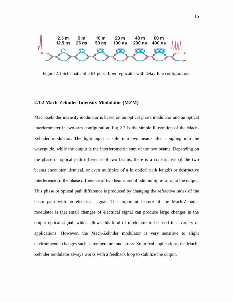
2.1.1 Fiber Replicator
To characterize single-shot events, an optical pulse can be replicated and averaged with
itself for better signal to noise ratio. Either a fiber resonator or a delay-line (retarding
pulse replicator) enables single-shot self-replication [1-2]. Due to the simple design, ease
of fabrication and constant signal amplitude, the delay-line is the preferred configuration.
The delay-line configuration is composed of a series of 2×2 fused-fiber splitters spliced
with differential delay fibers as illustrated in Fig 2.1. The length of the fiber in the Nth
stage depends on window time and the number of previous stages. In Fig 2.1, the unit
delay time is 12.5 ns (corresponding to 2.5 meters fiber), which means there will be a
total of 2N pulses replicated from the original signal pulse, and the time window for each
pulse is 12.5 ns. The unit delay time also specifies the maximum temporal pulse-width
for the signals. If the signal pulse-width is larger than the unit delay time, there will be
interference between neighboring pulses.
Ideally, the optical power of the original signal will be distributed evenly and all these
duplicates have the same amplitude. However, due to the fiber loss and the deviation
from a perfect 50/50 splitting ratio of the fiber couplers, there will be difference in the
amplitude of each pulse. Therefore, the amplitudes of these duplicated pulses will be
normalized or resized in the post-processing.
Page 41
15
Figure 2.1 Schematic of a 64-pulse fiber replicator with delay-line configuration.
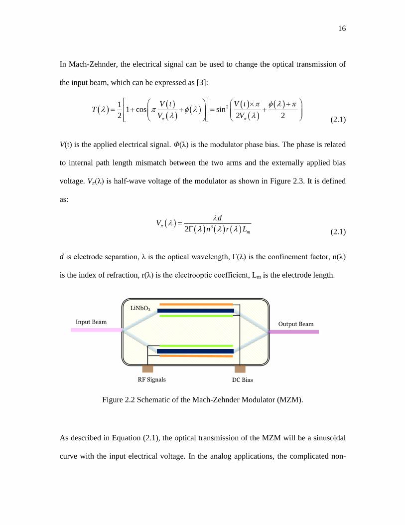
2.1.2 Mach-Zehnder Intensity Modulator (MZM)
Mach-Zehnder intensity modulator is based on an optical phase modulator and an optical
interferometer in two-arm configuration. Fig 2.2 is the simple illustration of the Mach-
Zehnder modulator. The light input is split into two beams after coupling into the
waveguide, while the output is the interferometric sum of the two beams. Depending on
the phase or optical path difference of two beams, there is a constructive (if the two
beams encounter identical, or even multiples of π in optical path length) or destructive
interference (if the phase difference of two beams are of odd multiples of π) at the output.
This phase or optical path difference is produced by changing the refractive index of the
beam path with an electrical signal. The important feature of the Mach-Zehnder
modulator is that small changes of electrical signal can produce large changes in the
output optical signal, which allows this kind of modulator to be used in a variety of
applications. However, the Mach-Zehnder modulator is very sensitive to slight
environmental changes such as temperature and stress. So in real applications, the Mach-
Zehnder modulator always works with a feedback loop to stabilize the output.
Page 42
16
In Mach-Zehnder, the electrical signal can be used to change the optical transmission of
the input beam, which can be expressed as [3]:
211 cos sin
2 2 2
V t V tT
V V
(2.1)
V(t) is the applied electrical signal. Φ(λ) is the modulator phase bias. The phase is related
to internal path length mismatch between the two arms and the externally applied bias
voltage. Vπ(λ) is half-wave voltage of the modulator as shown in Figure 2.3. It is defined
as:
32 m
dV
n r L
(2.1)
d is electrode separation, λ is the optical wavelength, Г(λ) is the confinement factor, n(λ)
is the index of refraction, r(λ) is the electrooptic coefficient, Lm is the electrode length.
Figure 2.2 Schematic of the Mach-Zehnder Modulator (MZM).
As described in Equation (2.1), the optical transmission of the MZM will be a sinusoidal
curve with the input electrical voltage. In the analog applications, the complicated non-
LiNbO3
Input Beam Output Beam
DC Bias RF Signals
Page 43
17
linear transfer function of the MZM is a disadvantage when the amplitude of the
electrical signal is comparable to Vπ [4]. To avoid this condition, the MZM is normally
operated in the linear range.
Figure 2.3 Schematic of a MZM operating in linear range. (The transmission vs. voltage
curve is plotted using Vπ= 5 V and Ф= - 0.4π.)
To operate in linear range, the DC bias of the MZM can be set to any quadrature point
with 50% transmission such as Vπ/2 which is shown as the pink spot in Figure 2.3. Around
Vπ/2 area, the optical transmission is almost linear with the voltage. When a small time
varying signal, V(t), is applied to the MZM (shown as the blue arrows in the figure), the
V
0 3 6 9 12 150
0.1
0.2
0.3
0.4
0.5
0.6
0.7
0.8
0.9
1
Voltage (V)
Tra
nsm
issio
n
Vπ
Vπ/2
V(t)
T
Page 44
18
optical transmission will change linearly with the RF voltage signal (shown as dark red
curve).
The uniaxial crystal lithium niobate (LiNbO3) is commonly used as the waveguide
material in the Mach-Zehnder modulators [5]. LiNbO3 based Mach-Zehnder modulators
have high switching speed (about 20 GHz) which makes them popular in modern
communication systems [6]. Recently, Silicon and polymers are also investigated as
waveguide materials for as fast as 40 GHz switching speed [7-8].
2.1.3 Wavelength division multiplexing (WDM)
In fiber-optical systems, wavelength-division multiplexing (WDM) is a technology which
multiplexes a number of optical carrier signals at different wavelengths onto a single
optical fiber. The WDM components multiply the capacity of the fiber-optical system by
the number of different wavelength channels.
Wavelength multiplexing components are divided into groups such as WDM, CDWDM
and DWDM based on wavelength spacing. WDMs or broad WDMs components
normally work on only two wavelength bands such as 980nm/1550nm and
1310nm/1550nm. The wavelength spacing of the conventional/coarse (CWDM)
wavelength-division multiplexing is 20nm. The International Telecommunication Union
(ITU) specifies eighteen CWDM wavelengths from 1271nm to 1611nm [9]. Dense
WDMs (DWDM) have much narrower wavelength spacing [10]. Practically employed
Page 45
19
DWDMs are normally spaced at 100GHz (approximately 0.8nm separation in wavelength)
[11]. DWDMs commonly work in the C-band wavelengths, which coincides with the
gain spectrum of EDFAs. So EDFAs have been widely used with DWDM systems to
compensate optical signal transmission loss in modern telecom networks.
To separate wavelengths, optical filters are used in WDMs to remove unwanted channels
or wavelengths such as residual pump powers and broad ASE background after EDFAs.
2.2 Erbium-doped fiber amplifier
An Erbium-doped fiber amplifier (EDFA) is a type of optical amplifier that uses Er-
doped fiber as gain medium to amplify optical signals. The amplification process is, in
essence, the process of stimulated emission of photons from dopant Er3+
ions in the Er-
doped fiber. The EDFA was first demonstrated by a group from the University of
Southampton and another group from AT&T Bell Laboratories at the same year [12-13].
An EDFA can work in a wide bandwidth (20-70nm) within the 1500-1600 nm
telecommunication bands. And it has the advantages of high gain (20-40 dB) and high
output power (>200 mW). Its amplification performance is insensitive to bit rate, input
power, pulse shape, and input wavelength. Because of these features, EDFAs have now
been widely used in modern telecommunications, especially those incorporating WDMs.
Page 46
20
2.2.1 Spectra of Er3+
dopant in silica fiber and cross sections
The electronic configuration of Erbium is 1s22s
22p
63s
23p
64s
23d
104p
65s
24d
105p
64f
126s
2.
The outer 5s and 5p shells effectively shield inner 4f electrons from significant
interaction with the local crystalline field associated with the charges on neighboring ions
in solid state configurations [14]. In a condensed form, the trivalent Er3+
is the most
stable state. In the ionic Er3+
state, two outer 6s electrons and one inner 4f electron are
removed, and then outer shell electronic configuration becomes 4f11
. 4I15/2 is the ground
state of Er3+
. The radiative transition 4I13/2→
4I15/2 of Er
3+ ion in silica fiber will emit
photons with wavelengths around 1.53 µm [15]. As there are many sublevels in both 4I13/2
and 4I15/2 as shown in Figure 2.4, the emitted photon wavelengths will range from about
1520nm to 1620nm. And this is the working principle of Er-doped fibers as gain media
for light amplifications. Typically the amplification process will include the initial
pumping of Er3+
ions from the ground state 4I15/2 to any higher energy level such as
4H11/2
[16-17]. The relaxation processes between 4H11/2 to
4I13/2 energy levels are predominantly
nonradiative decay. After fast and nonradiative relaxation or decay processes, the ions
will finally drop to metastable 4I13/2 state and be followed by a radiative emission by
4I13/2y→
4I15/2 transition, with a life time about 10 ms. This process is analogous to three-
level systems, especially when pumping at 980nm, 800nm and above [17]. However, we
will still treat 980nm pumped Er-doped fiber as two-level system in the simulations in
Chapter 4 for simplification. As the excited carriers in 4I11/2 are quickly depleted via
nonradiative transition 4I11/2 →
4I13/2, the two-level system is still a good approximation
[18].
Page 47
21
Figure 2.4 Energy level of Er3+
dopant in silica fiber [22].
For stimulated light amplification in gain media, the stimulated transition cross sections
are very important parameters. The stimulated transition cross sections include absorption
and emission cross sections. In this thesis, we will neglect excited-state absorption (ESA)
in our simulations (although the ESA phenomenon may occur in our system which we
will discuss in Chapter 3). ESA is the process where the upper level populations not only
amplify the input light via stimulated emission but also absorb the pump power and jump
to higher energy levels [19]. This process will decrease the pumping efficiency. ESA can
be neglected for 980nm pumping if the pump powers are not very high [18-21].
Absorption and emission cross sections are hypothetical areas (with the unit m-2
) used to
describe the possibilities of light being absorbed or emitted. These cross sections are
Page 48
22
different from geometrical cross sections in that they depend on the wavelength of the
incident light and the permittivity [23].
2.2.2 Three-level system
As mentioned in the last section, the amplification process in Er-doped fiber amplifier is
analogous to a three-level system. And therefore, we will simplify the amplification
process in EDFA into a three-level model and then further simplify the model into a two-
level system in the simulations in Chapter 4.
Figure 2.5 The three-level simplified system of Er3+
in glass.
The three-level system model is plotted in Figure 2.5. Energy level “1” is the ground state,
corresponding to energy level 4I15/2 in Er-doped fibers. Energy level “2” is the metastable
level, corresponding to energy level 4I13/2 in Er-doped fibers. Energy level “3” is the
energy level of excited photons, corresponding to 4I11/2 if pumping with 980nm light. The
( 4I11/2 )
1 ( 4I15/2 )
2 ( 4I13/2 )
3
υpσp
υsσs
Γ32
Γ21
Page 49
23
populations of each level are N1, N2 and N3. The incident light intensity flux at the
frequency corresponding to 1→3 transition is denoted as υp. This transition is the actual a
pumping or light absorption process used in the experiments described in Chapter 3. υs is
the signal flux of the 1→2 transition, corresponding to light emission process. σp and σs
are the corresponding transition cross sections. Г32 and Г23 are the transition possibilities
between level 3 and level 2, Г32 = Г23. In Er-doped fibers, this transition is a non-radiative
system with very fast decay time. Г21 and Г12 are the transition possibilities from level 2
to level 1, and similarly Г21 = Г12. In Er-doped fibers, it is actually the radiative transition
4I13/2→
4I15/2. The rate equations for the population changes are written as [24]:
121 2 1 3 2 1
221 2 32 3 2 1
332 3 1 3
p p s s
s s
p p
dNN N N N N
dt
dNN N N N
dt
dNN N N
dt
(2.2)
Under steady-state, there are no time-dependent variations of populations:
1 2 3 0
dN dN dN
dt dt dt (2.3)
And the total population N is given by:
1 2 3N N N N (2.4)
Based on Equation 2.3, 2.4 and 2.5, the population difference between 4I13/2 and
4I15/2 in
steady state is:
Page 50
24
212 1
21 2
p p
p p s s
N N
N
(2.5)
The population inversion occurs when N2 ≥ N1. So the threshold for lasing or
amplification is:
21
2
1th
p p
(2.6)
where τ2 is the lifetime of energy level 2, and τ2 = 1 / Г21. The pumping intensity is
defined as Ip = hυp υp. The power is defined as the product of intensity and effective area
P = Ip Aeff. So the threshold pumping power can be expressed as:
21
21
p eff p eff
th
p p
h A h AP
(2.7)
For a pumping wavelength of 980nm, with an absorption cross section σp = 2×10-21
cm2,
lifetime τ2 = 10 ms, effective area Aeff = 20 µm2 (5 μm diameter for core area) for single-
mode fibers, the threshold power is about 2 mW. This demonstrates one important
advantage for EDFAs, i.e. the low threshold pumping power for gain [18].
2.2.3 Steady-state gain
As defined in the last section, the pump (transition 1→3) and the signal (transition 2→1)
photon flux are:
Page 51
25
s
s
s
p
p
p
I
h
I
h
(2.8)
Assume the light propagation along with z direction, which is actually the optical axis of
the Erbium fiber, and without considering the transverse field along the fiber, which
simplifies this propagation process into a one-dimensional problem.
After a length of Δz of Er-doped fiber, the change of photon flux in both pump and signal
are:
2 1
3 1
ss s
p
p p
dN N
dz
dN N
dz
(2.9)
Combined with Equation 2.9 and Equation 2.6, the change of photon flux along the fiber
can be described as:
21
21
2
p p
pss s
p p s s
p s
I
hdII N
I Idz
h h
(2.10)
In terms of the above equation, we can find that the role of Er-doped fibers in optical
systems depends on the pump power and the cross section for the pumping wavelength. If
the numerator in the above equation is less than zero, for example a small pump power,
the Er-doped fiber is actually working as an attenuator in the system. The numerator
Page 52
26
must be larger than zero for real amplification, which results in the threshold condition
for pumping power Ith = hυp/σpτ2. For pump powers, we have the similar equation:
21
21
2
s s
p sp p
p p s s
p s
I
dI hI N
I Idz
h h
(2.11)
For convenience, the pump and the signal flux are normalized by pump threshold. The
new and normalized pump and signal flux are:
/
/
p p th
s s th
I I I
I I I
(2.12)
If the signal is far away from saturation, the signal propagation can be expressed in a
simple format:
0 exp
1
1
s s p
p
p s
p
I z I z
IN
I
(2.13)
αp is defined as gain coefficient. The signal gain (G) with specific length of Er-doped
fiber is defined as:
1010log0
s
s
I z LG
I z
(2.14)
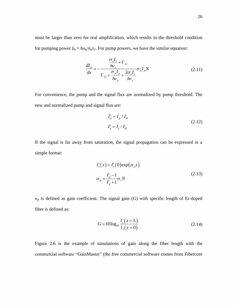
Figure 2.6 is the example of simulations of gain along the fiber length with the
commercial software “GainMaster” (the free commercial software comes from Fibercore
Page 53
27
Limited, for Erbium Doped Fiber Amplifier Simulation). The plots show the relation of
gain and pumping power for a 10m Er-doped fiber with 980nm pumping wavelength.
Although the commercial software can be used to calculate most of the parameters such
as gain, ASE and noise configuration, all those calculations are based on steady-state
conditions (Equation 2.4). If the signals are not CW or quasi-CW, the EDFA is not
operating under steady-state. Under these conditions, we cannot directly use the results
from the commercial software.
0 5 10 15 20 25 30 35 40 45 50
-40
-30
-20
-10
0
10
20
30
40
Pumping power (mW)
Ga
in (
dB
)
0 1 2 3 4 5 6 7 8 9 10
-5
0
5
10
15
20
25
30
35
Length (m)
Gain
(dB
)
(a) (b)
Figure 2.6 Simulation of the signal gain vs. pump power (a) and vs. the fiber length (b).
The signal is at 1550.116nm, pumping wavelength is 980nm, Er-doped fiber length is
10m, the input signal is -30dBm (0.001mW). This simulation was done with the software
“GainMaster” from Fibercore Limited with the single stage forward pumping setup.
2.2.4 Amplifier noise
Inevitably, all amplifiers degrade the signal-to-noise ratio (SNR) of the system because of
the extra random (no fixed polarization, phase, frequency and direction) amplified
Page 54
28
spontaneous emission (ASE). The extent of the degradation is quantified by the
parameter NF, noise figure. It is defined as [15-16]:
1010log in
out
SNRNF
SNR (2.15)
(SNR)in and (SNR)out are the input and output power signal-to-noise ratios, respectively.
For an amplifier with the gain G, the SNR of the input signal is given by [25]:
2
in
in
PSNR
h f
(2.16)
The (SNR)out can be expressed as:
2
2 4 2
d in in
outASE
R GP GPSNR
S h f
(2.17)
σ2 is the variance of photocurrent, Rd is the responsivity of an ideal photo detector with
unit quantum efficiency, SASE is the spectral density of ASE given by:
0 1ASE spS n h G (2.18)
nsp is the spontaneous emission factor, or the population-inversion factor defined as:
2
2 1
ssp
s p
Nn
N N
(2.19)
Substituting Equation 2.17-2.20 into Equation 2.16, the noise figure can be expressed as
[14-15]:
Page 55
29
10 10
2 1 110log 10log 2 3
sp
sp
n GNF n dB
G G
(2.20)
The approximation in the above equation is valid when gain G >> 1. Under ideal
conditions, all population at ground level (level 1) is inverted which makes N1 = 0 and
then nsp = 1. And therefore, 3 dB is the theoretical limit for noise figure in phase-
insensitive amplifiers.
Figure 2.7 Schematic of the experimental setup for the phase sensitive amplifier. Black
and blue lines represent optical and electrical connections, respectively. The inset plots
show the input spectra of phase-insensitive and phase-sensitive amplifications,
respectively. BER sensitivity was measured at port A and B by considering PSA as a pre-
or inline amplifier, respectively. CW, continuous wave; NFA, noise-figure analyzer; OSA,
optical spectrum analyzer; PM, phase modulator; PC, polarization controller; PZT,
piezoelectric transducer; PD, photodetector; TDL, tunable delay line; VOA, variable
optical attenuator; PRBS, pseudo-random bit sequence; BER, bit-error ratio; TX,
transmitter [33].
Page 56
30
Recently research on fiber amplifiers shows that phase sensitive amplifiers have a better
NF, a theoretical 0 dB noise figure (NF) [26]. Low NF has been achieved in both high
frequency (16GHz) and low frequency region [27-32]. The lowest NF that has been
achieved is 1.1 dB (the experimental setup is shown in Figure 2.7) [33]. Despite the
advantage of high NF, phase sensitive amplifiers are far more complicated systems than
phase insensitive amplifiers such as EDFAs, which limit their commercial applications.
2.2.5 Transient gain
The EDFA gain derived in Chapter 2.2.3 is based on the steady-state assumption. For the
steady-state assumption to be valid, the change of signal power should be slow compared
to the optical transit time of the gain media (Er-doped fibers).
However, this assumption will not be valid if there are sudden changes in the number of
channels or if the signal powers change rapidly. The first situation is quite normal in
modern optical network systems for signal channels add-on or drop-off or the sudden
failure of some components. The second situation happens in the DANTEEO system. The
typical signal waveform in the DANTEEO system is shown in Fig 2.8. Assuming the
length of the Er-doped fiber is 10 m with the refractive index 1.5. So the optical transit
time is 50 ns, while the signals in the DANTEEO system change amplitude within ~ns.
For such fast signal power changes, the EDFA is not working under steady-state range
but in transient range.
Page 57
31
50 60 70 80 90 100 110 1200
0.1
0.2
0.3
0.4
0.5
0.6
0.7
0.8
0.9
1
Time (ns)
Norm
aliz
ed A
mplit
ude
Figure 2.8 The typical signal pulse shape in the DANTEEO system. The left corner is a
whole train pulses generated by a fiber replicator.
A model for transient gain in EDFA has been derived and can deal with the gain
dynamics in the DANTEEO system based on the following assumptions [21, 34-35]:
The EDFA model is based on a two-level system. Although our system will be
more accurately simulated by a three-level model, a two-level system is still a
good approximation as the lift time of 4I11 is very short compared with our signal
time width and the life time of 4I13 .
We will neglect excited-state absorption. This has been stated in Chapter 2.2.1.
The gain spectrum is homogenously broadened and the time scale for such
broadening is much faster than any relevant optical process.
0 50 100 150 200 250 300 3500
0.1
0.2
0.3
0.4
0.5
0.6
0.7
0.8
0.9
1
Time (ns)
Norm
aliz
ed A
mplit
ude
Page 58
32
Gain saturation by ASE is negligible compared to the saturation by the signals.
This assumption is valid for the gain below 20dB. In our system, the gain is
normally below 20dB. Or the gain spectrum is adjusted by a holding channel so
that the gain will not be saturated by ASE even under higher gain. We will discuss
gain-flattening and the use of a holding channel in Chapter 3.
Signal power changes slowly compared to the transit time of light going through
the Er-doped fiber. In the DANTEEO system, the signals do not satisfy this
requirement. However, we use the finite difference method and divide the whole
fiber length into very small steps. During each small step (the step is 25ps or 50ps
in time), the signals (power changes in ~ns level) can be regarded as quasi-CW
sources.
The area of the Er-doped active region is small compared to the optical mode at
the signal wavelength. This assumption allows the overlap factor for signal
wavelength to be kept constant and independent of optical power.
The pumping wavelength is treated the same as the signal wavelengths only with
different emission and absorption coefficients.
Under these assumptions, the rate equation for the population in excited state N2 and the
photon propagation equation are [36]:
Page 59
33
2 2
10
2
( , ) ( , ) 1 ( , )
( , )( , ) ( , )
Ni
i
it eff
nn n n n n
N z t N z t P z tu
t N A z
P z tu N z t P z t
z
(2.21)
The γn and αn are emission and absorption constants defined as:
e
n t n n
a
n t n n
N
N
(2.22)
N2(z, t) is the fractional population of the upper state. Pi(z, t) is the optical power of the
pumping and/or signals, in units of number of photons per unit time. Nt is the doping
concentration of Er ions. Aeff is the effective fiber core area. τ0 is the life time of the
upper state population. Г is the overlap factor. σe and σ
a are the emission and absorption
cross sections for a specific wavelength. u is the unit vector, for forward direction u= +1,
for backward direction u= -1.
Page 60
34
Figure 2.9 An example of the transient response. Inset shows the same transient response
over a long time period. Δt expresses the time span for changing the gain by 0.5 dB from
the initial value after changing the input channel number [37].
Figure 2.9 is an example of dynamic gain with channel add-on using Equations 2.21 and
2.22 [37]. As shown in Figure 2.9, the simulations for transient gains deal with the
signals varying in the μs range. The signals in the DANTEEO system vary in the ns range,
as shown in Figure 2.8. The red rectangle in Figure 2.9 represents the time window that
we are interested in as the signals in the DANTEEO system always change amplitudes in
a very fast way. We will apply this model (Equation 2.21) in the simulations of transient
gains for fast signals with amplitudes changing in the ns range in Chapter 4.
The region we
are interested
Page 61
35
Reference
1. M. Komanec, P. Honzatko, S. Zvanovec,, “Single-Shot All-Optical Sampling
Oscilloscope Using a Poplarization-Maintaining Resonator for Pulse Replication”,
Microwave and Optical Technology Letters, vol.52, No. 11, 2010.
2. C. Dorrer, J. Bromage, J. D. Zuegel, “Highdynamic-range Single-shot Cross-correlator
Based on An Optical Pulse Replicator”, Opt. Express, vol. 12(18), pp. 13534-13544,
2008.3. J. A. Valdmanis, G. Mourou, and C. W. Gabel, “Picosecond electrooptic
sampling system”, Appl. Phys. Lett., vol. 41, pp. 211, 1982.
3. S. Dubovitsky, W. H. Steier, S. Yegnanarayanan and B. Jalali, “Analysis and
Improvement of Mach-Zehnder Modulator Linearity Performance for Chirped and
Tunable Optical Carriers”, Journal of Lightwave Technology, vol. 20, No. 5, May 2002
4. Tutorial Note #5: “Modulation Schemes”, SHF Communication Technologies AG,
www.shf.de/communication/support/tutorial_notes/getfile/72/288/
5. R. Kashyap, “Fiber Bragg Gratings”, 2nd ed., Academic Press, Boston, 2009.
6. Abd El-Naser A. Mohamed, Mohamed A. Metawe'e Ahmed Nabih Zaki Rashed and
Amira M. Bendary, “Recent Progress of LiNbO3 Based Electrooptic Modulators with
Non Return to Zero (NRZ) Coding in High Speed Photonic Networks”, International
Journal of Information and Communication Technology Research, vol. 1, No.2, 2011.
7. M Iodice, G Cocorullo, F.G Della Corte, I Rendina, “Silicon Fabry-Perot filter for
WDM systems channels monitoring”, Optics Communication, vol. 183, No. 5-6, 2000.
8. L. V. Bartkiv, Ya. V. Bobitski, “Design and optimization of concave diffraction
grating for WDM multi/demultiplexer”, LFNM*2010 International Conference on Laser
& Fiber-Optical Networks Modeling, Sevastopol, Ukraine, 2010.
9. ITU-T Recommendation G. 694.2, Spectral grids for WDM applications: CWDM
wavelength grid
10. ITU-T Recommendation G. 694.1, Spectral grids for WDM applications: DWDM
wavelength grid
11. http://www.motorola.com/staticfiles/Video-
Solutions/_Documents/static%20files/WDM%20CWDM%20DWDM%20Segmentation
%20Primer.pdf
12. R.J. Mears, L. Reekie, I.M. Jauncey, D. N. Payne: “Low-noise Erbium-doped fiber
amplifier at 1.54μm”, Electron. Lett, vol. 23, pp.1026–1028, 1987.
Page 62
36
13. E. Desurvire, J. Simpson, P.C. Becker, “High-gain erbium-doped traveling-wave fiber
amplifier”, Optics Letters, vol. 12, No. 11, 1987.
14. W. J. Miniscalco, “Erbium-Doped Glasses for Fiber Amplifiers at 1500 nm”, Journal
of Lightwave Technology, vol. 9, No. 2, Feb 1991.
15. Govind P. Agrawal, “Applications of Nonlinear Fber Optics”, Academic Press, 2001.
16. P. C. Becker, N. A. Olsson, J. R. Simpson, “Erbium-doped fiber amplifiers:
fundamentals and technology”, Academic Press, 1999.
17. E. Desurvire, “Erbium-doped Fiber Amplifier: Principles and Applications”, Wiley,
New York, 1994.
18. C. Randy Giles, and Emmanuel Desurvire, “Modeling erbium-doped Fiber
amplifiers”, Journal of Lightwave Technology, vol. 9, No. 2, Feb 1991.
19. P. R. Morkel and R. I. Laming, “Theoretical modeling of erbium-doped fiber
amplifiers with excited-state absorption”, Optics Letters, vol. 14, No. 19, 1989.
20. R. I. Laming, S. B. Poole, and E. J. Tarbox, “Pump excited-state absorption in
erbium-doped fibers”, Optics Letters, vol. 13, No. 12, 1988.
21. A. A. M. Saleh, R. M. Jopson, J. D. Evankow, and J. Aspell, “Modeling of gain in
erbium-doped fiber amplifiers”, IEEE Photon Technol Lett, vol. 2, pp. 714-717, Oct 1990.
22. Picture from:
http://people.seas.harvard.edu/~jones/ap216/lectures/ls_2/ls2_u5/ls2_unit_5.html
23. R.G. Newton, “Scattering Theory of Waves and Particles”, McGraw Hill, 1966.
24. P. C. Becker, N. A. Olsson and Jay R. Simpson, “Erbium-Doped Fiber Amplifiers:
Fundamentals and Technology”, Lucent Technologies, 1999.
25. G.P. Agrawal, “Fiber-optic communication systems”, 4th
edition, Wiley, 2010.
26. A. Zavatta, J. Fiurasek, M. Bellini, “A high-fidelity noiseless amplifier for quantum
light states” , Nature Photonics. vol. 5, pp.52-60, 2011.
27. S.K. Choi, M. Vasilyev, P. Kumar, “Noiseless optical amplification of images”, Phys.
Rev. Lett, vol. 83, pp.1938–1941, 1999.
28. W. Imajuku, A. Takada, Y. Yamabayashi, “Low-noise amplification under the 3 dB
noise figure in high-gain phase-sensitive fibre amplifier”, Electron. Lett, vol. 35,
pp.1954–1955, 1999.
29. K. Croussore, G. Li, “Phase regeneration of NRZ-DPSK signals based on symmetric-
pump phase-sensitive amplification”, IEEE Photon. Technol. Lett, vol. 19, 864–866 2007.
Page 63
37
30. O.K. Lim, V. S. Grigoryan, M. Shin, P. Kumar, “Ultra-low-noise inline fiber-optic
phase-sensitive amplifier for analog optical signals”, in Proceedings of the Optical Fiber
Communications Conference (OFC/NFOEC 2008), San Diego, USA, paper OML3, 2008.
31. R. Tang, “Gain characteristics of a frequency nondegenerate phase-sensitive fiber-
optic parametric amplifier with phase self-stabilized input”, Opt. Express, vol. 13, pp.
10483–10493 2005.
32. J. Kakande, “Detailed characterization of a fiber-optic parametric amplifier in phase-
sensitive and phase-insensitive operation”, Opt. Express, vol. 18, pp. 4130–4137, 2010.
33. Z. Tong, C. Lundström, P. A. Andrekson, C. J. McKinstrie, M. Karlsson, D. J.
Blessing, E. Tipsuwannakul, B. J. Puttnam, H. Toda, L. Grüner-Nielsen, “Towards
ultrasensitive optical links enabled by low-noise phase-sensitive amplifier”, Nature
Photonics, vol. 5, pp.430-436, 2011.
34. Y. Sun, G. Luo, J. L. Zyskind, A. A. M. Saleh, A. K. Srivastava, and J.W. Sulhoff,
“Model for gain dynamics in erbium-doped fiber amplifiers,” Electron. Lett., vol. 32, No.
16, 1996.
35. R. M. Jopson and A. A. M. Saleh, “Modeling of gain and noise in erbium-doped
fiber amplifiers,” SPIE Fiber Laser Sources and Amplifiers III, vol. 1581, pp. 114–119,
1991.
36. Y. Sun, J. L. Zyskind, and A. K. Srivastava, “Average Inversion Level, Modeling and
Physics of Erbium-Doped Fiber Amplifiers”, IEEE Journal of Selected Topics in
Quantum Electronics, vol. 3, No. 4, Aug 1997.
37. Hirotaka Ono, and Makoto Shimizu, “Analysis of Gain Dynamics of Erbium-Doped
Fiber Amplifiers for Wavelength-Division-Multiplexing Networks”, IEEE Journal of
Quantum Electronics, vol. 39, No. 4, Apr 2003.
Page 64
38
Chapter 3: Erbium-doped fiber amplifiers (EDFAs) for
NIF DANTE system
In this chapter, we will describe the EDFA configurations for low noise NIF DANTEEO
system diagnostics. The comparison of different EDFA setups will be discussed based on
noise levels and the pulse shape restoration.
3.1 EO diagnostic system for NIF DANTE (NIF DANTEEO)
3.1.1 The EO system configuration
This EO data acquisition system is built to enhance SNR so that it can be a viable
alternative to the current system. The whole system is packed in a black box for system
stability and low noise. The picture is shown in Fig 3.1. The configuration of the EO
system is shown in Fig 3.2, followed by the detailed description of the system.
Figure 3.1 NIF DANTEEO system packed in a black box.
Page 65
39
3.1.2 System specifications of the components
A four channel DFB laser (from Optilab) is used as the source laser. The wavelength of
each channel is tunable within some range. The tuning step is 0.2nm. The details are
listed in Table 3.1.
Table 3.1 Parameters for the DFB laser
Channel Output Power (dBm) Wavelength (nm) Wavelength Tuning Range (nm)
Ch. 1 12.34 1547.73 1546.12 – 1549.65
Ch. 2 12.19 1552.52 1550.92 – 1554.15
Ch. 3 12.77 1554.13 1552.41 – 1555.72
Ch. 4 16.40 1557.35 1555.65 – 1558.93
The actual wavelength from the laser has a little deviation from the panel readout. If the
output power is changed the output wavelength will change as well. So the wavelengths
we noted on this proposal are the wavelengths we measured with a calibrated spectrum
analyzer.
The configuration of the DANTEEO system is in Figure 3.2. The detailed explanation
follows:
All laser wavelengths come from a four channel CW DFB laser system. PC represent in-
line polarization controller. AOM represents an acoustic optical modulator. MZ
represents Mach-Zehnder modulator.
Page 66
40
(a)
(b) (c)
Figure 3.2 The schematic of the EO system for NIF DANTE (a). The thick black arrows represent electrical signals and the
thin black arrows represent optical signals. Schematics of 4× (b) and 2× (c) replicator used in the DANTE system shown in (a).
40m
200ns 80m
400ns 20m
100ns
Page 67
41
90/10 is the beam splitter, in which 10 percent of the input light is used as a feedback for
the MZ bias-dithering, control system and the remaining 90 percent of the input light
goes to DWDM component. RF is the radio frequency signal from an electronic signal
generator which is used to drive the Mach-Zehnder. The 1×3 splitter is the one input and
three output RF connector. OSC Chan is the channel of the oscilloscope. EDFA is the
commercial EDFA with details described later in this chapter. Replicator is a fiber
replicator using the delay line configuration to create identical copies of the input pulses.
There are total three output ports of this 8× fiber replicator. One port connected to
detector #1 is from the 4× replicator, so the output will be four pulses for each
wavelength. Another 4× output was connected to a 2× input port on panel. The other
output from the 4x replication stage was connected to Detector #1 which was a DSC
402DC photodetector with amplification. One of the outputs of the 8x replication stage
was connected to Detector #2 which was a DSC 50S photodetector without any
amplification.
The optical paths for both 1557nm and 1552nm were almost the same except that
1552nm had a delay line before the DWDM wavelength combiner. First, the AOM carves
the CW laser output into a 100 ns pulse with a repetition rate of 39 Hz. This repetition
rate was chosen much less than the 1-kHz dither frequency to stabilize the MZM. The
Mach-Zehnder imprints the signal to be measured onto the square pulse into a window
about 30ns wide at the top of the square pulse. The AOM has high extinction ratio so that
it can create a clear background with zero intensity beyond the signal. This high
extinction ratio is needed to propagate the pulses through the replicator without optical
Page 68
42
interference. However, the AOM suffers from a rather long arise time (15 ns), which
forces a minimum time window of about 50ns for the signals in the DANTEEO system.
The Mach-Zehnder modulator has lower extinction ratio, however it has a high
bandwidth (up to 10 GHz). As our system is designed for signals up to 6GHz, the MZ
modulator provides sufficient bandwidth margins for all the measurements the system
will make. So the AOM and MZ are combined to create low background, fast optical
pulses. As the efficiency of pulse carving of the Mach-Zehnder modulator is related to
the polarization, a polarization controller and a polarizer were installed before the MZ to
get maximum modulation. The delay line added in 1552nm optical path was used to
avoid temporal overlap of two wavelengths in the fiber replicator.
Due to the long rise time of the first AOM that was used (about 40ns), the original system
was designed for signals with time width about 160ns. So the 4× replicator (shown in
Figure 3.2(b)) was built for about a 200ns time window. A faster AOM (about 15ns arise
time) was used in the later experiments, which can narrow the signal time window to
about 60ns. Accordingly, we built another 2× replicator as shown in Figure 3.2(c). One
output of the 4× replicator was connected to the input of the 2× replicator. Together with
4× replicator, this replicator combination can create total 8 duplicate signals with 100ns
time window.
The commercial EDFA needs a CW input of about 1mW, otherwise it will turn-off
automatically. So the third wavelength, 1547nm, is used to keep the commercial EDFA
active before the signal pulse train arrives. The output #2 of the replicator shown in
Page 69
43
Figure 3.2 was left unconnected in the original system. The EDFA developed for this
thesis used this output to monitor the pulse shape differences between the input and
output of the EDFA.
The DWDM component used in the EO system was a 200GHz-spacing 8-channel
multiplexer. The operating wavelengths for each channel were 1547.72nm, 1549.32nm,
1550.92nm, 1552.52nm, 1554.13nm, 1555.75nm, 1557.36nm and 1558.98nm.
Figure 3.3 Schematic of commercial Mach-Zehnder bias controller [1].
Figure 3.4 Calibration of both MZ modulators.
Page 70
44
The MZ modulators use the electro-optic effect to modulate the phase of the incoming
light. And therefore, they are very sensitive to environmental conditions such as
temperature and stress. To ensure a stable bias point in the transmission curve and a
stable pulse shape output, a commercial Mach-Zehnder bias controller was used to
maintain the optical bias at the negative quadrature point. Similar to the commercial
EDFA, the MZM bias controller also needs a CW signal because the dither controller
assumes harmonics of the dither frequency are always on. The schematic illustration is
shown in Figure 3.3. This extra CW signal channel plays an important role in the system
because it affects the gain dynamics of EDFAs, which will be discussed in section 3.3.3.
To apply MZM in the DANTEEO system, Vπ of both Mach-Zehnder modulators was
carefully calibrated. The calibration process was done through the measurement of
transmitted light intensities (transmission) versus the applied voltage. The results are
shown in Figure 3.4.
As we mentioned in Chapter 2, the fiber replicator will distribute the optical power into
several nearly identical. The amplitude of the output signal (for example, at output #2 in
Figure 3.2) was too small to be detected with a standard photodiode. Although the SNR
can be enhanced by averaging the identical pulses, the overall SNR will suffer from weak
signals because the SNR is proportional to the signal power. So we need an amplifier to
provide enough gain to measure the signal without introducing too much noise [1]. In the
DANTEEO system, an amplified photodetector was used after the 4× replicator to
amplify the signals electronically. However, this detector did not provide enough gain to
make measurements with a SNR of at least 100. We need an optical signal amplifier to
Page 71
45
get amplified analog optical signals as it is hard to estimate the analog pulse-shape
distortion from amplified photodetectors. An EDFA was used in the DANTEEO system
to amplify signals beyond the noise floor of the photodiodes. The EDFAs can amplify
signals within large wavelength range (about 40nm) in telecomm band. They have low
noise and high output powers. The maintenance of EDFAs is also comparatively easy as
they do not demand complicated alignment techniques.
We have both C-band and L-band Erbium-doped fibers in lab. The L-band Erbium-doped
fibers came from Thorlabs. The C-band Erbium-doped fibers came from 3M, the
absorption and emission cross sections are shown in Figure 3.5. We will use the
estimated absorption and emission cross sections based on parameters from this figure to
calculate the dynamic gain in Chapter 4.
1450 1500 1550 1600 1650-1
0
1
2
3
4
5
6
7
8
Wavelength (nm)
Inte
nsity (
dB
/m)
Absorption Coefficient
Emission Coefficient
Figure 3.5 Absorption and emission coefficients in the C-band Erbium-doped fiber [2].
Page 72
46
3.2 Characterization of the commercial EDFA
In order to exceed the noise and gain performance of the current commercial EDFA
(MANLIGHT), we took a set of data with different pumping laser currents in the unit of
mA [1]. The parameters of this commercial EDFA are listed in Table 3.2.
Table 3.2 Parameters of the commercial EDFA [1].
Parameters Specification Unit
Pump Laser Wavelength 975 nm
Pump Laser Power 300 mW
Pump Laser current for 20 dBm Output power 471.0 mA
Amplifier Gain 5-30 dB
Saturated Output power 20 dBm
Figure 3.6(a) is the 4× pulse train with the photodetector (DSC403DC) which has a gain
M = 2-7. The amplified photodetector was used to monitor the system and also to
compare with the optical amplified signals (the signals out of this detector are electrically
amplified). Figure 3.6(b) is the 8× pulse train from the commercial EDFA amplified with
a pumping laser current of 90mA. This is the small signal gain regime where the EDFA is
unlikely to introduce pulse shape distortions. The inserted small plots on the upper right
corner of Fig 3.6(a) and (b) are the individual pulses. The dynamic range (DR) is defined
as the ratio between the largest and the smallest signal amplitudes. The dynamic range in
Figure 3.6(b) for the commercial EDFA pumped with 90mA is about 6, far away from
Page 73
47
system design requirements (above 4000). The low dynamic range and low SNR as well
should be attributed to weak signals and noise from the amplifier.
1200 1400 1600 1800 2000 2200 2400-0.005
0
0.005
0.01
0.015
0.02
0.025
Time (ns)
Am
plit
ud
e (
V)
(a)
1200 1400 1600 1800 2000 2200 2400 2600 2800 3000 32000
0.002
0.004
0.006
0.008
0.01
0.012
0.014
0.016
0.018
0.02
Time (ns)
Am
plit
ud
e (
V)
(b)
Figure 3.6 The pulse trains from 4× output with an amplified photodetector (a) and 8×
output amplified by the commercial EDFA with 90 mA pumping current (b).
1160 1170 1180 1190 1200 1210 1220 1230-0.005
0
0.005
0.01
0.015
0.02
0.025
Time (ns)
Am
plit
ud
e (
V)
1340 1350 1360 1370 1380 1390 14000
0.002
0.004
0.006
0.008
0.01
0.012
0.014
0.016
Time (ns)
Am
plit
ud
e (
V)
Page 74
48
As all components of the commercial EDFA were sealed in the black box, the only way
to enhance the SNR and dynamic range was to get higher amplification. To increase the
amplification, the pumping laser current of the EDFA was increased. The results were
recorded using a digital oscilloscope. As the working conditions of the laser source and
the Mach-Zehnder modulators may vary with time, the actual optical powers of the input
and amplified signals will also vary. So the ratio between the maximum amplitude of the
amplified signals and the 4× output signals as recorded on the DSC 403DC photodiode
was used to characterize the amplification of the commercial EDFA.
80 100 120 140 160 180 2000
0.5
1
1.5
2
2.5
3
3.5
4
Pumping Current (mA)
Am
plit
ud
e R
atio
Figure 3.7 The relationship between the amplitude ratio between 4× output signals and
the EDFA pumping current. Curves come from two different measurements.
We measured the output powers of the EDFA with the pumping laser currents from 90
mA to 190 mA (190 mA is the maximum pumping current set for the experiments to
Page 75
49
avoid gain saturation). For each pumping current, we measured 10 times with 1 min
separation in time. The amplitude ratio in Figure 3.7 is the average of the ratio between
the optically amplified signals and the electrically amplified signals. The black and blue
curves in Figure 3.7 come from two measurements (at different days) with different
Mach-Zehnder RF voltages. From this figure, the amplification of the commercial EDFA
is quite stable. The EDFA gain is linearly proportional to the pumping current.
1000 1200 1400 1600 1800 2000 2200 2400 2600 2800 30000
0.02
0.04
0.06
0.08
0.1
0.12
0.14
0.16
Time (ns)
Am
plit
ud
e (
V)
Figure 3.8 The amplified signals with the pumping current at 190 mA.
Page 76
50
0 10 20 30 40 50 60
0
0.02
0.04
0.06
0.08
0.1
0.12
0.14
0.16
GPIBczha
Built-in EDFA 190mA
2.hdf MZ 1
Time (ns)
Am
plit
ud
e (
V)
(a)
0 10 20 30 40 50 600
50
100
150
200
250
300
350
400
GPIBczha
Built-in EDFA 190mA
2.hdf MZ 1
Time (ns)
SN
R
(b)
Figure 3.9 The pulses realigned and normalized based on the first pulse modulated by
Mach-Zehnder #1 (a). The red curve represents the first pulse, the blue curve represents
the last pulse, and the green curve is the averages of each eight replicas. (b) The
calculated SNR vs. time corresponding to the pulses in (a).
Background level
Page 77
51
0 10 20 30 40 50 60
0.01
0.02
0.03
0.04
0.05
0.06
0.07
0.08
GPIBczha
Built-in EDFA 190mA
2.hdf MZ 2
Time (ns)
Am
plit
ud
e (
V)
(a)
0 10 20 30 40 50 600
50
100
150
200
250
GPIBczha
Built-in EDFA 190mA
2.hdf MZ 2
Time (ns)
SN
R
(b)
Figure 3.10 The pulses realigned and normalized based on the first pulse modulated by
Mach-Zehnder #2 (a). The red curve represents the first pulse, the blue curve represents
the last pulse, and the green curve is the averages of each eight replicas. (b) The
calculated SNR vs. time corresponding to the pulses in (a).
Background level
Page 78
52
1500 1510 1520 1530 1540 1550 1560 1570 1580 1590 1600-70
-60
-50
-40
-30
-20
-10
Wavelength (nm)
Inte
nsity (
dB
m)
Figure 3.11 The spectrum of the amplified signals shown in Figure 3.8. The ASE
background is continuous. The duty cycle for the holding channel is about 100%, for two
signals channels (1552nm and 1557nm) is 6.6×10⁻³
%.
Figure 3.8 is the waveform reading from the oscilloscope. Figure 3.9(a) and Figure 3.10(a)
are the aligned pulses. For each set of pulses (8 pulses) in Figure 3.8, we aligned them
together and rescaled the pulses to have the same amplitude as the first pulse in each set.
Figure 3.9(b) and Figure 3.10(b) are the calculated SNR(t). The formula used to calculate
SNR is:
Avg V NSNR
Std V
(3.1)
Avg (V) is the averaged amplitude value of eight pulses, Std (V) is the standard deviation
at each point in time of all eight rescaled pulses, N is the number of replicas. Figure 3.9(b)
and Figure 3.10(b), the SNR for Mach-Zehnder #1 is about 150, for Mach-Zehnder #2 is
about 75. The background level is about 0.02 V. The amplification of the commercial
Page 79
53
EDFA added extra CW background level of 0.02 V, about 8 μW. This CW background
mostly comes from ASE. The SNRs in Figure 3.9 and Figure 3.10 are the best SNRs that
can be achieved with this commercial EDFA without distortions. Figure 3.11 is the
spectrum. The three peaks are associated with the two signal wavelengths and the one
holding channel at 1547.72nm. The duty cycle of the holding channel is about 100%. The
duty cycle for the two signal channels is 6.6×10⁻³
%. The broadband background across
the whole spectrum can be attributed to ASE.
3.3 Characterization of EDFAs
This section describes a variety of EDFAs that were constructed as alternatives to the
commercial unit and discusses the relationship between the EDFA performance (gain and
noise) and a variety of component parameters.
3.3.1 EDFAs with L-band Er-doped fiber and multi-stage configuration
For a single stage EDFA, there are several different configurations including forward, bi-
direction and backward based on pumping schemes. In the DANTEEO system, the signal
to be amplified was very weak and barely able to be detected even with an amplified
photodetector. Therefore, based on simulations with commercial software shown in
Figure 2.6, a long Er-doped fiber was not needed. In other words, the amplification
depends on the power of the input signal, in a single-stage configuration. Besides, the
Page 80
54
noise or the SNR is also proportional to the amplitude of the amplified signal. In order to
obtain high SNRs, we need high amplifications which are impossible for single-stage
configurations with very weak input signals. There are two choices available, a
regenerative EDFA or a multi-stage EDFA. The regenerative EDFA is similar to an all-
fiber ring laser configuration, in which an optical pulse circulates in a fiber cavity where
it efficiently gains energy by repeated passes in the gain fiber [3-10]. The advantage of
the regenerative EDFA is the high gain with compact size. However it has a relatively
high noise level as both signal pulses and the noise (mainly ASE) circulate and are
amplified in the loop. For the current DANTEEO system, we prefer high SNRs even at
the cost of lower amplification. So we chose another solution, the multi-stage EDFA.
Different multi-stage configurations were tried to decrease the noise. Generally speaking,
there are several sources of the noise. The most apparent source of the noise is ASE,
amplified spontaneous emission. Light originating from ASE has a spectrum
approximately the same as the gain spectrum of the Er-doped fibers which means the
ASE covers a wide wavelength range. The ASE has no fixed frequency in time domain
and no fixed phase relation relative to the signals. Therefore, ASE is very hard to remove
in phase-insensitive optical amplifiers like an EDFA. This kind of noise is random in
time and polarization. Another source of the noise is the EDFA pumping laser. The
population inversion in Er-doped fibers does not reach 100%, there are still some residual
powers from the 980 nm pumping laser at the output. As the pumping laser is CW, this
type of noise is CW and can be mostly eliminated by bandpass filters, or dropped off by
WDMs as shown in Fig 3.12 and 3.13. Another noise source comes from the bandwidth
Page 81
55
of the photodetector, also called white noise. To reduce the white noise, the most efficient
method is to choose a photodetector with the bandwidth only a little larger than the signal
frequency in time domain. The signal frequency in our current DANTEEO system is 39
Hz, the bandwidth of our current detector is 10GHz. So if we choose a photodetector with
much lower bandwidth, we can increase the SNR dramatically. However, the
DANTEEO system is designed for finally up to 6GHz signals. So currently we ignore
this type of noise.
The inevitable noise, or the base noise, is the initial signal noise. Different configurations
of EDFAs are designed to decrease only the extra noise from the amplification process.
The noise from the original signal is amplified simultaneously along with the signal. So
the fiber replicator can actually increase and decrease the noise in this DANTEEO system.
It produces the replicas for mathematical averaging to increase the SNR. On the other
hand, the extra amplifier such as the EDFA has to be used to amplify the signal which
degrades the SNR. The final SNR, either improved or degraded by the fiber replicator,
depends on the competition between these two effects. So our target is to suppress the
noise introduced by the EDFA for the particular signal pulse train generated by the
DANTEEO system.
Page 82
56
Figure 3.12 Two-stage dual forward pumping EDFA experimental setup.
Figure 3.12 is the two-stage dual forward pumping EDFA configuration. The BWDM
after the first stage was used as a filter to narrow the wavelength range. As the passing
band for the BWDM is 1554.89-1563.89nm, we used the BWDM to remove the ASE
background beyond the passing band. The residual powers from the 980nm pumping
laser after the first stage was deliberately neglected as this residual pumping power can
be used (or recycled) in the second stage amplification. The WDM after the second stage
was used to drop the pumping channel and the DWDM was used to further narrow the
bandwidth of the amplified signals. The signal wavelengths 1555.73nm and 1557.36nm
were specifically chosen that these two wavelengths were within the pass band of the
BWDM and were exactly the same wavelengths as two of the DWDM channels. The
pump power for the first stage was 60 mW and the second stage was 40.4 mW. The
pumping laser used in the lab to build the EDFAs described in this Chapter came from
Amonics Limited (980nm Benchtop FP Laser Source, Model: AFP-980-300-B-FA).
Page 83
57
Table 3.3 Optical Parameters of the EDFA pumping laser [11].
Parameter Units Test Data
Centre wavelength nm 974.56
Output power @ centre wavelength mW > 290
FWHM nm 0.418
Output stability (over 8 hours) dB < ±0.02
Figure 3.13 Two-stage forward and backward pumping EDFA experimental setup.
There are three possible pumping schemes for two-stage EDFAs, dual forward pumping
(such as the EDFA configuration shown in Figure 3.12), forward and backward pumping
(such as the EDFA configuration shown in Figure 3.13) and dual backward pumping
schemes. As the individual pulses in the pulse train have different polarizations, the
polarization related components such as Faraday isolators are not applicable in the
DANTEEO system. In the fiber-optical systems, the Faraday isolator is used to allow the
transmission of light in only one direction and prevent the damages from unwanted
feedback light. In order to prevent the system damage from the backward traveling pump
light for the system without isolators, the backward pumping schemes for the first stage
Page 84
58
were not considered appropriate in the DANTEEO system. The backward pumping
scheme can be used in the second stage because the first stage will deplete the excess
pump light from the second stage. Therefore, the final gain and noise performance were
critically dependent on the pumping scheme of the second stage. The forward pumping
scheme on the second stage, which occurs primarily near the input end of the Er-doped
fiber, has the characteristic of low gain and low noise level. While the backward
pumping scheme on the second stage, which occurs primarily near the output end of the
fiber, is supposed to be high gain and high noise level. This high noise level comes from
the strong backward ASE power at the output end of the fiber. These two different
configurations were tried to determine which one is better for the DANTEEO system.
Figure 3.14 - 3.20 are the experimental results and the calculated SNR distributions for
these two configurations.
0 200 400 600 800 1000 1200 1400 1600 1800 2000-0.02
0
0.02
0.04
0.06
0.08
0.1
0.12
Time (ns)
Am
plit
ud
e (
V)
Figure 3.14 The amplified signals with the configuration shown in Figure 3.12.
Page 85
59
0 10 20 30 40 50 600
0.02
0.04
0.06
0.08
0.1
0.12GPIB
czha
Forward pump with BWDM and DWDM 2.5m+5m
60mW+40.4mW6.hdf MZ 1
Time (ns)
Am
plit
ud
e (
V)
(a)
0 10 20 30 40 50 600
50
100
150
200
250GPIB
czha
Forward pump with BWDM and DWDM 2.5m+5m
60mW+40.4mW6.hdf MZ 1
Time (ns)
SN
R
(b)
Figure 3.15 The pulses (from Figure 3.14) realigned and normalized based on the first
pulse modulated by Mach-Zehnder #1 (a). The red curve represents the first pulse, the
blue curve represents the last pulse, and the green curve is the averages of each eight
replicas. (b) The calculated SNR vs. time corresponding to the pulses in (a).
Background ≈ 0.005 V
Page 86
60
0 10 20 30 40 50 600
0.01
0.02
0.03
0.04
0.05
0.06
0.07
0.08GPIB
czha
Forward pump with BWDM and DWDM 2.5m+5m
60mW+40.4mW6.hdf MZ 2
Time (ns)
Am
plit
ud
e (
V)
(a)
0 10 20 30 40 50 600
20
40
60
80
100
120
140GPIB
czha
Forward pump with BWDM and DWDM 2.5m+5m
60mW+40.4mW6.hdf MZ 2
Time (ns)
SN
R
(b)
Figure 3.16 The pulses (from Figure 3.14) realigned and normalized based on the first
pulse modulated by Mach-Zehnder #2 (a). The red curve represents the first pulse, the
blue curve represents the last pulse, and the green curve is the averages of each eight
replicas. (b) The calculated SNR vs. time corresponding to the pulses in (a).
Background ≈ 0.005 V
Page 87
61
0 200 400 600 800 1000 1200 1400 1600 1800 2000-0.02
0
0.02
0.04
0.06
0.08
0.1
0.12
0.14
0.16
Time (ns)
Am
plit
ud
e (
V)
Figure 3.17 The amplified signals with the configuration shown in Figure 3.13.
Page 88
62
0 10 20 30 40 50 60-0.02
0
0.02
0.04
0.06
0.08
0.1
0.12
0.14
0.16GPIB
czha
Forward pump with DWDM and WDM dropoff 2.5m+5m
60mW+30.4mW3.hdf MZ 1
Time (ns)
Am
plit
ud
e (
V)
(a)
0 10 20 30 40 50 60
0
50
100
150
200
250
300GPIB
czha
Forward pump with DWDM and WDM dropoff 2.5m+5m
60mW+30.4mW3.hdf MZ 1
Time (ns)
SN
R
(b)
Figure 3.18 The pulses (from Figure 3.17) realigned and normalized based on the first
pulse modulated by Mach-Zehnder #1 (a). The red curve represents the first pulse, the
blue curve represents the last pulse, and the green curve is the averages of each eight
replicas. (b) The calculated SNR vs. time corresponding to the pulses in (a).
Background
level
Page 89
63
0 10 20 30 40 50 600
0.005
0.01
0.015
0.02
0.025
0.03
0.035
0.04GPIB
czha
Forward pump with DWDM and WDM dropoff 2.5m+5m
60mW+30.4mW3.hdf MZ 2
Time (ns)
Am
plit
ud
e (
V)
(a)
0 10 20 30 40 50 60
0
10
20
30
40
50
60GPIB
czha
Forward pump with DWDM and WDM dropoff 2.5m+5m
60mW+30.4mW3.hdf MZ 2
Time (ns)
SN
R
(b)
Figure 3.19 The pulses (from Figure 3.17) realigned and normalized based on the first
pulse modulated by Mach-Zehnder #2 (a). The red curve represents the first pulse, the
blue curve represents the last pulse, and the green curve is the averages of each eight
replicas. (b) The calculated SNR vs. time corresponding to the pulses in (a).
Background
level
Page 90
64
0 0.02 0.04 0.06 0.08 0.1 0.120
20
40
60
80
100
120GPIB
czha
Forward pump with BWDM and DWDM 2.5m+5m
60mW+40.4mW6.hdf
Amplitude (V)
SN
R
MZ1
MZ2
(a)
0 0.02 0.04 0.06 0.08 0.1 0.12 0.140
20
40
60
80
100
120
140
160GPIB
czha
Forward pump with DWDM and WDM dropoff 2.5m+5m
60mW+30.4mW3.hdf
Amplitude (V)
SN
R
MZ1
MZ2
(b)
Figure 3.20 Comparisons of the SNRs at different signal amplitudes (a) dual forward
pumping scheme, the configuration shown in Figure 3.12 (b) forward and backward
pumping scheme, the configuration shown in Figure 3.13. The dashed blue lines are the
fittings of the SNR vs. Amplitude. The dashed and point green lines in the two figures are
the SNR at the signal amplitude 0.1 V reading from the oscilloscope.
Page 91
65
Figure 3.14-3.19 are the experimental results from the configurations described in Figure
3.12 and Figure 3.13. In Figure 3.20, the SNR vs. signal amplitude were plotted for two
different configurations. MZ1 and MZ2 in the Figure 3.20 represent the two signal
channels which were modulated by two individual MZMs, and shown in Figure 3.14 and
3.17 as two pulse trains (each has 8 duplicated pulses). From both plots in Figure 3.20,
the SNRs for the two signal channels agreed well with each other as the red and black
dots overlaps. When the signal amplitude equals 0.1V (corresponding to 2.5 mW), the
forward and backward configuration has higher SNR (above 100) than dual forward
configuration (about 90), which are shown as green dashed lines in Figure 3.20. For
small signals (about 0.03V, corresponding to 0.83mW), EDFAs with dual forward
configurations also have lower SNR. The background levels for both configurations are
around 0.005V, smaller than the commercial EDFA. As a whole, the backward and
forward configuration has better noise performance than both forward pumping schemes.
As shown in Figure 3.20, the SNRs are not uniform with the signal amplitudes. In Figure
3.20 (a), the SNRs for the signals with 0.1 V in amplitudes have a variation of ±15
around 90. The error bars of the SNR mostly come from the ASE, shot noise and
accidental environmental noise.
Besides the gain and noise performance, the pulse-shape fidelity during amplification
process is also an important factor in the EDFA design for the DANTEEO system.
Page 92
66
150 200 250 300 350 400 450-0.2
0
0.2
0.4
0.6
0.8
1
1.2
Time (ns)
Am
plit
ud
e (
v)
Lab-built EDFA
Commercial EDFA
Figure 3.21 Comparisons of pulse shape with the signals amplified by two EDFAs.
Figure 3.21 is the comparison of two EDFAs. The amplitudes were both normalized to
1V to compare the pulse shape. The lab-built EDFA, shown as the black line, is the same
configuration in Figure 3.12 with the pump power at 75 mW for the first stage and 18
mW for the second stage. The commercial EDFA, shown as the red line was pumped at
180 mA. From this figure, we can find two major problems for the commercial EDFA.
The pulse was broadened during amplification process. And the commercial EDFA did
not do well with analog signals that have high frequencies. The high frequency is
typically defined as being equal to 0.33/Δt where Δt is the temporal structure of interest.
We found the amplified pulses from the commercial EDFA have the uniform pulse
shapes with those from lab-built EDFAs and amplified photodetectors while below
130mA (the gain is about 2-5 dB). Above 130mA pumping current, the pulses from the
commercial EDFA started distorting such as those shown in the Figure 3.21.
Page 93
67
For different configurations and fiber components we tried in the experiments, we found
that
We cannot use polarization related fiber optics in our setup such as isolators.
Because the individual pulses in the pulse train have different polarizations, the
polarization related optics cannot modulator the individual pulses evenly.
For the above reason, backward pumping cannot be used in a one-stage
configuration, or in the first stage of a two-stage configuration. But the backward
pumping in the second-stage of a two-stage configuration as shown in Figure 3.13
can increase the SNR without introducing strong backflow of energy toward the
MZM‟s.
Because the Er-doped fiber has wide amplification spectrum, the output signal
after the EDFA has much wider spectrum than the input signal. In addition, there
is typically some residual pump light present at the output of the Er-doped fibers.
Bandpass filters can increase the SNR and largely decrease the background level.
In the two configurations in Figure 3.12 and 3.13, either a WDM after the second-
stage was used to remove the residual pump light or a backward pumping scheme
was used to decrease the pump light reaching the photodiode. BWDM and
DWDM spectral filters were used to narrow the spectrum of the signal and rule
out the noise.
Compared with the commercial EDFA, the constructed EDFAs have two
advantages, lower background and higher pulse-shape fidelity. Under the similar
amplification, our EDFAs have about ¼ the background level (0.005 V,
Page 94
68
corresponding to 0.125 mW) of the commercial EDFA (0.02 V, corresponding to
0.5 mW). Besides, the commercial EDFA has pulse-shape distortions under large
amplification (above pumping current at 130 mA) for the pulses with high
frequencies (such as the pulses shown in Figure 3.21). By comparison, our lab
EDFAs do not have obvious pulse-shape distortion even under the highest
amplification and with signals having high modulation frequencies.
3.3.2 Performance of EDFAs with L-band and/or C-band Er-doped fibers
The previous section emphasized on the effect of different configurations on the gain and
noise performance of EDFAs. The Er-doped fibers used in the previous experiments were
all L-band Er-doped fibers from Thorlabs. This chapter will focus on the effect of
different Er-doped fibers (C-band and L-band) with different material properties on the
gain and noise performance of EDFAs.
Figure 3.22 Two-wavelength pulse trains were generated via AOMs to simulate the
electro-optic measurement system input to the EDFA.
Page 95
69
For simplification, an acousto-optic modulator (AOM) was used to generate the pulse
train for each wavelength. The setup configuration is shown in Figure 3.22. The two
pulse-trains from two different wavelengths have a time separation length about the time
length of a whole pulse train to prevent the crosstalk. A DWDM was used to combine
two signals.
To compare the effect of C-band and L-band fibers on EDFA performance, a simple one-
stage forward pumping configuration, as shown in Figure 3.23, was used. The pumping
wavelength was 980nm and the second WDM was used to drop off the residual pumping
power.
Figure 3.23 A single-stage EDFA configuration for testing different types of optical fiber.
Page 96
70
1400 1600 1800 2000 2200 2400 26000
0.02
0.04
0.06
0.08
0.1
0.12
0.14
Time (ns)
Am
plit
ud
e (
v)
C-band Er-doped fiber with 25mW pumping
Figure 3.24 Signals from a single-stage EDFA with C-band Er-doped fibers. The typical
waveform read directly from the oscilloscope, the pump power is 25mW at 980nm.
Background
level
Page 97
71
1500 1510 1520 1530 1540 1550 1560 1570 1580 1590 1600-70
-65
-60
-55
-50
-45
-40
-35
-30
Wavelength (nm)
Am
plit
ud
e (
dB
m)
40mW
35mW
30mW
25mW
20mW
15mW
10mW
7mW
(a)
1545 1550 1555 1560-60
-55
-50
-45
-40
-35
-30
Wavelength (nm)
Am
plit
ud
e (
dB
m)
40mW
35mW
30mW
25mW
20mW
15mW
10mW
7mW
(b)
Figure 3.25 The spectra for EDFAs with C-band Er-doped fibers (a) with different
pumping powers (b) zoom-in the spectra at signal wavelengths from 1545nm-1560nm.
The length of the C-band Er-doped fiber in Figure 3.24 is 3-meter. The input signals were
about -44 dBm (1547nm) and -42dBm (1557nm). The repetition rate is 39 Hz. Two
sharp peaks (at 1547nm and 1557nm) in the spectra (Figure 3.25) were the signal
Page 98
72
wavelengths. From the oscilloscope waveform, the background is about 0.034 V and the
dynamic range is less than 7:1. A WDM was used to remove the residual 980nm pump
light. The background and the noise level should be mostly attributed to the strong ASE.
Figure 3.25 show the spectra at the output. With the increase of the pump power, the
spectral background and the amplitudes of the ASE peaks around 1530nm also increase.
Although the spectral data were recorded with the pump power to 40mW, the waveform
data was only recorded up to pump powers of 26mW. Above that level, the ASE signals
were too strong and the photodetector were saturated. A nonlinear effect, presumably
excited-state absorption, was observed with high pump powers (about 200mW and
above). There was, very obviously, green light coming out of the EDFA in this situation.
Page 99
73
1600 1800 2000 2200 2400 2600-0.05
0
0.05
0.1
0.15
0.2
0.25
0.3
Time (ns)
Am
plit
ud
e (
v)
L-band Er-doped fiber with 100mW pumping
(a)
1500 1510 1520 1530 1540 1550 1560 1570 1580 1590 1600
-80
-75
-70
-65
-60
-55
-50
-45
-40
-35
-30
Wavelength (nm)
Am
plit
ud
e (
dB
m)
140mW
120mW
100mW
80mW
60mW
40mW
(b)
Figure 3.26 Signals from single-stage EDFA with the L-band Er-doped fiber. (a) The
typical waveform reading from the oscilloscope, pump power is 100mW. (b) The spectra
under different pump powers. The red circle shows the spectral hole burning (SHB).
Figure 3.26 are the oscilloscope waveform and the spectra of a 4.5-meter L-band Er-
doped fiber single-stage EDFA. Compared with the C-band Er-doped fiber, EDFAs with
SHB
Background level
Page 100
74
L-band Er-doped fibers had much lower background (≈0.02 V, corresponding to 0.5 mW)
and higher dynamic range (≈ 12:1). However, increasing the pump power for higher gain
resulted in spectral hole burning (SHB) [11]. As shown in Figure 3.26, the SHBs are
located at about 1554nm and the amplitude is about 0.5 dB with 140mW pump power.
The gain between 1547nm-1560nm becomes flatter with the increasing pump power up
to about 120mW. The peak of the gain around 1530nm also moves very slightly toward
(less than 0.5nm, almost invisible in the zoom size of the spectra plots in the thesis)
shorter wavelengths with increasing pump powers. By comparison, the peak of the gain
around 1530nm in the EDFAs with C-band Er-doped fibers did not move with the change
of the pump powers. The EDFA with the L-band Er-doped fiber also has gain
compression around 1540nm which might come from the gain saturation around 1530nm
[12]. The magnitude of the gain compression is nearly independent on the pump power.
By comparison, the EDFA with C-band Er-doped fibers does not have obvious gain
compression.
Page 101
75
1500 1510 1520 1530 1540 1550 1560 1570 1580 1590 1600-80
-75
-70
-65
-60
-55
-50
-45
-40
-35
-30
Wavelength (nm)
Am
plit
ud
e (
dB
m)
L-band 4.5m Er-doped fiber pumping with 80mW
C-band 3m Er-doped fiber pumping with 25mW
(a)
1540 1542 1544 1546 1548 1550 1552 1554 1556 1558 1560-55
-50
-45
-40
-35
-30
Wavelength (nm)
Am
plit
ud
e (
dB
m)
L-band 4.5m Er-doped fiber pumping with 80mW
C-band 3m Er-doped fiber pumping with 25mW
(b)
Figure 3.27 The comparison of C- and L- band Er-doped fibers. (a) The whole spectra
range from 1500nm to 1600nm. (b) Spectra around 1540nm to 1560nm.
Figure 3.27 are the comparisons of the spectra obtained with two different types of Er-
doped fibers. The spectra for comparing the Er-doped fibers were taken at moderate gains
(about 15-25 dB depending on different types of Er-doped fibers). The spectrum analyzer
Page 102
76
measures the CW optical power, so it does not accurately reflect the gain of the transient
signals. However, useful information can still be gathered from this instrument. The
EDFA with C-band Er-doped fibers had much higher ASE background, about 10 dB
higher in short wavelengths (around 1510nm) and 3dB in long wavelengths (1590nm).
However the peak of its ASE gain (around 1530nm) was much weaker than L-band Er-
doped fibers. From this point of view, the filter included in the single stage EDFA (as
shown in Figure 3.23) will work more efficiently with L-band Er-doped fibers in
removing the ASE background. This is because the ASE gain spectrum is concentrated
far from the signal wavelengths. Also, the L-band Er-doped fiber has a much flatter gain
within the band of interest (1547-1559 nm) than the C-band Er-doped fiber. However the
L-band Er-doped fiber experiences the SHB at about 1554nm (the affected wavelengths
range from 1553nm to 1554.5nm), which is actually one of the ITU-200 channels used at
the DANTEEO system.
Page 103
77
1600 1800 2000 2200 2400 2600-0.1
0
0.1
0.2
0.3
0.4
0.5
0.6
0.7
0.8
Time (ns)
Am
plit
ud
e (
V)
L-band +C-band Er-doped fiber with 100 mW pumping
(a)
1500 1510 1520 1530 1540 1550 1560 1570 1580 1590 1600-70
-65
-60
-55
-50
-45
-40
-35
-30
-25
Wavelength (nm)
Am
plit
ud
e (
dB
m)
120mW
100mW
80mW
60mW
40mW
(b)
Figure 3.28 Signals from the single-stage EDFA with L-band + C-band Er-doped fiber. (a)
The typical waveform reading from the oscilloscope, pumping power is 100mW. (b) The
spectra for different pump powers.
Figure 3.28 includes the signal waveform and spectra from an EDFA with both L-band
and C-band Er-doped fibers. The two types of Er-doped fibers were directly connected
together via fiber connectors. The signals went through the L-band Er-doped fibers first
Background level
Page 104
78
and then followed by the C-band Er-doped fibers. From the spectral plots, this type of
mixed Er-doped fibers had characteristics that are the sum of individual fibers, such as
gain compression around 1540nm, gain slope from 1542nm and flattened gain between
1550nm and 1557nm. From the oscilloscope waveform, this mixed fiber is closer to the
C-band fiber with its characteristics of high gain and high noise.
Page 105
79
1600 1800 2000 2200 2400 2600-0.05
0
0.05
0.1
0.15
0.2
0.25
0.3
0.35
0.4
0.45
Time (ns)
Am
plit
ud
e (
v)
C-band + L-band Er-doped fiber with 100mW pumping
(a)
1500 1510 1520 1530 1540 1550 1560 1570 1580 1590 1600-80
-70
-60
-50
-40
-30
-20
Wavelength (nm)
Am
plit
ud
e (
dB
m)
120mW
100mW
80mW
60mW
40mW
(b)
Figure 3.29 Signals from single-stage EDFA with C-band + L-band Er-doped fibers. (a)
The typical waveform reading from the oscilloscope, pumping power is 100mW. (b) The
spectra with different pumping power. The blue circle illustrates the spectral
characteristic of parasitic oscillations.
Figure 3.29 includes the signal waveform and the spectra from an EDFA with both C-
band and L-band Er-doped fibers. The Erbium gain medium was also composed of a
Background level
Page 106
80
directly connected two types of Er-doped fibers. This configuration is different from that
shown in Figure 3.28, in that the C-band fiber came first and followed by the L-band Er-
doped fiber. The signal waveform is closer to an L-band Er-doped fiber with its low noise
and moderate gain. Comparing the spectra of the two types of mixed Er-doped fibers, the
C+L type has high ASE gain (around 1530), steeper gain spectra in the 1547-1559nm
band and exhibits SHB with high pump powers. The C+L type also had lower
background level (≈ 0.02 V, corresponding to 0.5 mW) than the L+C type (0.05V,
corresponding to 1.25 mW). The 1530nm gain peak under 120mW was rather noisy, as
shown in the blue circle in Figure 3.29(b). This phenomenon probably came from the
parasitic oscillations within the C-band Er-doped fiber due to the reflections from the end
faces. As the experiments shown in the initial part of this Chapter, the C-band Er-doped
fiber has very low threshold pumping power (about several mW) compared with the L-
band Er-doped fiber. When the 120mW pump power was launched into the C-band Er-
doped fiber, both the signal and the ASE (especially the ASE peak wavelength of
1530nm) undergo signification amplifications. Because of the Fresnel reflections of the
fiber ends, the fibers will become a gain cavity for ASE signal oscillations. The
oscillation frequency will be different from that of the signals. So if the oscillation signals
are strong enough, the spectrum will have a modulated characteristic as illustrated in the
blue circle of Figure 3.29(b). The parasitic oscillations also affect the oscilloscope
waveform as seen by a second signal at a different modulation frequency from the 39Hz
trigger, as shown in Fig 3.30. This signal oscillates asynchronously with the triggered
Page 107
81
signal that triggers the oscilloscope. This phenomenon occurs very frequently in single-
stage EDFAs with backward pumping schemes.
0 50 100 150 200 250 300 350 400
0.02
0.03
0.04
0.05
0.06
0.07
0.08
0.09
0.1
0.11
Time (us)
Am
plit
ud
e (
V)
Figure 3.30 Free running ASE signals. The left small plot is the corresponding spectral
measurement.
1500 1510 1520 1530 1540 1550 1560 1570 1580 1590 1600-60
-55
-50
-45
-40
-35
-30
-25
-20
-15
-10
Wavelength (nm)
Inte
nsity (
dB
m)
Real Signals
ASE Signals
Page 108
82
1500 1510 1520 1530 1540 1550 1560 1570 1580 1590 1600-75
-70
-65
-60
-55
-50
-45
-40
-35
-30
Wavelength (nm)
Am
plit
ud
e (
dB
m)
2.5m C-band + 3m L-band Er-doped fiber with 80mW pumping
2.5m C-band + 3m L-band Er-doped fiber with 60mW pumping
3m L-band + 2.5m C-band Er-doped fiber with 80mW pumping
3m L-band + 2.5m C-band Er-doped fiber with 60mW pumping
(a)
1500 1510 1520 1530 1540 1550 1560 1570 1580 1590 1600-80
-75
-70
-65
-60
-55
-50
-45
-40
-35
-30
Wavelength (nm)
Am
plit
ud
e (
dB
m)
4.5m L-band Er-doped fiber pumping with 80mW
3m C-band Er-doped fiber pumping with 25mW
3m C-band + 2.5m L-band Er-doped fiber pumping with 80mW
2.5m L-band + 3m C-band Er-doped fiber pumping with 80mW
(b)
Figure 3.31 Comparisons of the EDFA gain spectrum using different Er-doped fibers.
Figure 3.31(a) is the comparison of two different types of mixed fibers. From this plot
and the waveforms in the previous pictures, the gain of the mixed fiber seems to be the
weighted average of the constituent fibers with the first fiber that the signal is launched
Page 109
83
into having the greatest weight. The noise performance seems dominated by the end fiber.
Compared with the L+C mixed fiber, the C+L fiber has lower gain and lower noise as its
ASE gain spectrum is more concentrated and lower than the C+L type. In the C+L
configuration, the L-band fiber works like a weak filter which lowers the gain of the
spectral wings. The combination of fiber lengths and pump powers illustrated in Figure
3.31(b) are the best choices of all four types of the Er-doped fiber configurations used in
a single-stage forward pumping EDFA.
Based on these experiments, the C-band fiber has the highest gain and the highest noise,
the L-band fiber has lower gain and the lowest noise, the C+L fiber has moderate gain
and moderate noise, and the L+C fiber has moderate to high gain and moderated to high
noise. The L+C configuration seems to be a good choice for the DANTEEO system.
Additional experiments were done to extend the single-stage EDFA results into the
double-stage EDFA configuration. The spectra of double-stage EDFAs are very close to
the spectra of single-stage EDFAs. For example, the spectrum of a double-stage EDFA
with L-band Er-doped fibers in the first stage and second stage is very close to the single-
stage EDFA with only L-band Er-doped fiber. Very good gain and noise performance
were obtained with a double-stage EDFA having the C-band Er-doped fiber in the first
stage and the L-band Er-doped fiber in the second stage. The waveform is shown in
Figure 3.32. We used a 15dB attenuator after the original signals (as shown in black in
the Figure 3.2) to reduce the signals into the levels similar as those coming out of the
replicator. About 30dB of amplification was obtained with moderate pump powers (about
Page 110
84
80 mW forward pumping for the first stage and 60 mW backward pumping for the
second stage).
200 300 400 500 600 700 800 900 1000-0.1
0
0.1
0.2
0.3
0.4
0.5
0.6
0.7
0.8
Time (ns)
Am
plit
ud
e (
v)
Original Signal (-15dB)
Amplified Signal
Figure 3.32 The oscilloscope waveform for a double-stage EDFA with C+L configuration.
The two pulse trains (either in black or in red) come from different wavelengths.
3.3.3 The addition of a holding channel and its effect on EDFA spectrum
As we can find from almost all spectra in the previous sections, there exists the effect of
gain saturation by ASE signals (around 1530nm). The gain coefficient of a
homogeneously broadened gain medium can be expressed as [14]:
0
2 2
21 /a s
gg
T P P
(3.2)
g0 is the peak value, ω is the frequency of the light, ωa is the atomic transition frequency,
P is the optical power of the signal and Ps is the saturated power. From this equation, the
Page 111
85
value of the gain coefficient will decrease when the signal is close to saturation. So the
gain saturation actually limits the energy-extraction efficiency [15].
In order to surpass the gain saturation from ASE, a channel with a quasi-CW signal was
added (referred to as the “holding channel”). Then a large amount of inverted population
was used to amplify the holding channel, in a controllable configuration, before the gain
can be saturated by the ASE.
0 0.5 1 1.5 2 2.5 3
x 10-6
0
0.5
1
1.5
2
2.5
3
3.5
Time (s)
Am
plit
ud
e (
a.u
.)
Holding Chanel: 1547.8nm
Leading Chanel: 1557.4nm
Trailing Chanel: 1552.6nm
Figure 3.33 Waveforms of holding and signal channels used in the electro-optic data
acquisition system.
Figure 3.33 are the temporal profiles of three channels in the DANTEEO system. Red
and blue lines are the two signal channels with different wavelengths (1552.6nm and
1557.4nm). The black line shows the holding channel. When there were no EO signals,
the holding channel was “on”; while the EO signal carrier pulses were “on”, the holding
channel was turned off to prevent crosstalk with the signal channels. The “on and off”
Amplitude of the
holding channel
Page 112
86
status of the holding channel was controlled through a MZM which couples a polarizer in
its input. For simplification, a polarization controller was added before the MZM to
adjust the amplitude (optical power) of the input light after the polarizer. The polarization
controller gave a coarse control of the optical power of holding channel.
1500 1510 1520 1530 1540 1550 1560 1570 1580 1590 1600-70
-60
-50
-40
-30
-20
-10
Wavelength (nm)
Inte
nsity (
dB
m)
Without 1547.72nm channel
minimum power of 1547.72nm channel
maximum power of 1547.72nm channel
Figure 3.34 The gain spectra of the signals as a function of the holding channel power.
The amplitude of the ASE peak decreased with the increasing of the holding channel
powers, as shown in Figure 3.34. The gain through 1547nm to 1559nm band is flatter.
Further increasing of the power of the holding channel would decrease the ASE peak so
that gain saturation by ASE can be avoided.
Page 113
87
Reference
1. W. R. Donaldson, C. Zhao, L. Ji, R. G. Roides, K. Miller, B. Beeman, “A single-shot,
multiwavelength electro-optic data-acquisition system for ICF applicationsa”, Review of
Scientific Instruments, vol. 83, No. 10, Oct 2012.
2. 3M datasheets for C- and L-band fibers with part number FS-ER-7A28 and FS-ER-
7B28.
3. A. Zavatta, J. Fiurasek and M. Bellini, “A high-fidelity noiseless amplifier for quantum
light states” , Nature Photonics. vol. 5, pp.52-60, 2011.
4. S.K. Choi, M. Vasilyev and P. Kumar, “Noiseless optical amplification of images”,
Phys. Rev. Lett, vol. 83, pp.1938–1941, 1999.
5. W. Imajuku, A. Takada and Y. Yamabayashi, “Low-noise amplification under the 3
dB noise figure in high-gain phase-sensitive fibre amplifier”, Electron. Lett, vol. 35,
pp.1954-1955, 1999.
6. K. Croussore and G. Li, “Phase regeneration of NRZ-DPSK signals based on
symmetric-pump phase-sensitive amplification”, IEEE Photon. Technol. Lett, vol. 19, pp.
864-866, 2007.
7. O.K. Lim, V. S. Grigoryan, M. Shin and P. Kumar, “Ultra-low-noise inline fiber-optic
phase-sensitive amplifier for analog optical signals”, in Proceedings of the Optical Fiber
Communications Conference (OFC/NFOEC 2008), San Diego, USA, paper OML3, 2008.
8. R. Tang, “Gain characteristics of a frequency nondegenerate phase-sensitive fiber-
optic parametric amplifier with phase self-stabilized input”, Opt. Express, vol. 13, pp.
10483-10493 2005.
9. J. Kakande, “Detailed characterization of a fiber-optic parametric amplifier in phase-
sensitive and phase-insensitive operation”, Opt. Express, vol. 18, pp. 4130-4137, 2010.
10. Z. Tong, C. Lundström, P. A. Andrekson, C. J. McKinstrie, M. Karlsson, D. J.
Blessing, E. Tipsuwannakul, B. J. Puttnam, H. Toda and L. Grüner-Nielsen, “Towards
ultrasensitive optical links enabled by low-noise phase-sensitive amplifier”, Nature
Photonics, vol. 5, pp.430-436, 2011.
11. Amonics Limited, User‟s Manual for 980nm Benchtop FP Laser Source, Model:
AFP-980-300-B-FA.
12. Maxim Bolshtyansky, “Spectral Hole Burning in Erbium-Doped Fiber Amplifiers”,
Jounal of Lightwave Technology, vol. 21, No. 4, Apr 2003.
Page 114
88
13. M. Tachibana, R. I. Laming, P. R. Morkel and D. N. Payne, “Gain cross saturation
and spectral hole burning in wideband erbium-doped fiber amplifiers”, Optics Lett, vol.
16, No. 19, Oct 1991.
14. P. W. Milonni and J. H. Eberly, “Lasers”, Wiley New York, 1988.
15. G. P. Agrawal, “Applications of Nonlinear Fiber Optics”, Academics Press, 2001.
Page 115
89
Chapter 4: Numerical simulations of transient gains for
EDFAs in the DANTEEO system
This chapter presents a simplified model for the dynamic gain in an EDFA [1]. Because
the signals in the DANTEEO system are analog signals, the temporal profile of the gain
is also of interest. If the gain is not temporally uniform, the pulse shape fidelity will
decrease during the amplification process.
4.1 Simulation method
As stated in Chapter 2 section 2.2.5, the Equations set 4.1 (the same as Equation 2.21 in
section 2.2.5) should be used to calculate the transient gain. The first equation in
Equation 4.1 is a rate equation. The first term on the right side of the equation describes
the effect of spontaneous emission related to the population in the excited-state, while the
second term describes the effect of total optical power related to the inverted population.
2 2
10
2
( , ) ( , ) 1 ( , )
( , )( , ) ( , )
Ni
i
it eff
nn n n n n
N z t N z t P z tu
t N A z
P z tu N z t P z t
z
(4.1)
The second equation in Equation 4.1 is the light propagation equation, which has been
largely simplified by Saleh from its original complicated style including sets of coupled
partial differential equations [2-3]. The equation assumes “n” simultaneous optical
Page 116
90
channels in the EDFA. The pump light is also regarded as an optical channel. From this
point of view, the pumping and the signals mutually affect the EDFA gain to the extent
that depends on their emission (γ) and absorption (α) coefficients, and the propagation
direction (u).
The finite difference method is used for numerical simulation. The signals are assumed to
only travel in the forward direction. Each time step permits only a very small propagation
length within the Er-doped fiber, for example 5mm per step. The transit time for 5mm
fiber is 25ps assuming the refractive index of the fiber is 1.5. Typical optical signals
change much more slowly (almost an order of magnitude slower). Under these
assumptions, the Equation 4.1 is applicable in the simulation of the DANTEEO system.
In the finite difference method, the signals were decomposed into segments in time
domain while the fiber was decomposed in space domain. For each small forward step
(Δz) in fiber, we will calculate the optical power for each small segment of the signal (Δt).
After going through a length of fiber equal to M×Δz for each Δt (the total length of the
pulse train is supposed to be N×Δt), we will reconstruct the signal and get the final
amplified signal. This process is shown in Fig 4.1. In the figure, a sequence of colored
boxes below the left original signal waveform represents the time segments Δt. The blue
boxes below the “Fiber” represent the length step Δz in fiber. The multiple arrays of
colored boxes below the right amplified signal waveform represent the amplified signals
for each time segment. The signal amplitudes after an EDFA are assumed to increase. So
we use more boxes in each Δt.
Page 117
91
Figure 4.1 Schematic of the finite difference method in the calculation of the EDFA gain.
The numerical solution of the differential equations requires the boundary/initial
conditions for N2 (z, 0) and Pp (z, 0), assuming there are no signals launching in the fiber
at initial time. The initial conditions can be calculated through the steady-state solution of
the Equation set 4.1[4-5]:
2 2
0
2
,( , ) ( , ) 10
( , )( , ) ( , )
p
i
t eff
p
n n n n p
P z tN z t N z tu
t N A z
P z tu N z t P z t
z
(4.2)
The Equation set 4.2 assumes there is only one pumping source for each fiber. We also
assume there is no other light source propagating (signals) in the fiber. The “ui”
represents the direction of pumping which equals “+1” for forward pumping and “-1” for
backward pumping. The steady-state condition requires that the partial derivative of time
equals zero. Then the upper-state population can be calculated from the rate equation:
M×Δz
0 1000 2000 3000 4000 5000 60000
0.5
1
1.5
2
2.5
3
3.5
Time (ns)
Am
plit
ude (
a.u
.)
Holding Channel: 1547.8nm
Leading Channel: 1557.4nm
Trailing Channel: 1552.6nm
0 1000 2000 3000 4000 5000 60000
0.5
1
1.5
2
2.5
3
3.5
Time (ns)
Am
plit
ude (
a.u
.)
Holding Channel: 1547.8nm
Leading Channel: 1557.4nm
Trailing Channel: 1552.6nm
Signal In Signal Out Fiber
N×Δt N×Δt
Original
Signal Amplified
Signal
Page 118
92
0
2
p
i
t eff
PN z u
N A z
(4.3)
Nt is the Erbium doping concentration. Replacing N2 in the propagation Equation 4.2 with
the Equation 4.3, the change of pump power along the fiber can be expressed as:
2 0 ( )p p
i i n p
t eff
P Pu u P z
z N A z
(4.4)
By solving this ordinary differential equation, we can obtain Pp(z, 0) and N2 (z, 0) by
replacing Pp(z, 0) back into Equation 4.3.
The transient gain is calculated by accumulating the gain of each small segment of the
signals going through each small piece of fiber. The whole process is shown in Figure 4.2.
At the last step, we will normalize both the original and amplified signal and compare the
amplitude difference of these two waveforms. The difference of the normalized
amplitude, if it exists (pulse-shape difference ≠ 0), is the distortion of the pulse-shape. As
the measurement of original electrical signal is based on the unfolding of the optical
signal, any distortion in the pulse-shape of the optical signal will result in deformed
reconstruction of the original electrical signal.
Page 119
93
Figure 4.2 The schematic of the finite-difference method applied in the calculation of
transient gain in EDFAs.
Calculation boundary conditions of
N2(z, 0), Pp(z, 0)
2 0N
t
0
pP
t
Get N2 (z, 0) and Pp (z, 0)
Decompose Fiber and Signals into small
segments in length and time
Calculate the gain for each signal
segments going through the fiber
Reconstructure the signal
Normalize both original and amplified
signals and calculating the difference in
amplitude (Distortion)
Page 120
94
4.2 Simulation parameters
The simulation requires the fiber parameters, including emission and absorption
coefficients for the pump and the signal wavelengths, the doping concentration, the fiber
core area and the spontaneous decay time.
1450 1470 1490 1510 1530 1550 1570 1590 1610 1630 1650-5
0
5
10
15
20
Wavelength (nm)
Absorp
tion a
nd E
mis
sio
n C
oeff
icie
nt
(dB
/m)
C-band: Absorption (Alpha) (dB/m)
C-band: Emission (g*) (dB/m)
L-band: Absorption (Alpha) (dB/m)
L-band: Emission (g*) (dB/m)
880 900 920 940 960 980 1000 1020 1040 1060 1080-2
0
2
4
6
8
10
12
Wavelength (nm)
Ab
so
rptio
n (
Alp
ha
) (d
B/m
)
L-band
C-band
(a) (b)
Figure 4.3 Absorption and Emission Coefficients of C- and L-band Erbium-doped fibers
at working wavelengths (a) and pump wavelengths (b). Data comes from [5].
From the data sheet, we can get emission and absorption coefficient (plotted in Figure 4.3)
and the fiber core area (Mode diameter = 5.26 μm). The spontaneous time is assumed to
be 10 ms [2-4]. However, the erbium doping concentration ranges from 9.0×10²³
ions/m3
to 6.0×1026
ions/m3 from a variety of references. But neither the 3M data sheets for the
particular fibers that were used nor the commercial software (such as GainMaster)
provides this important parameter. So a moderate doping concentration 4×1024
ions/m3
was used in the simulation in this Chapter. The absorption at 1550nm provided by the 3M
Page 121
95
data sheet is 3.32 dB/m [5]. The calculated absorption coefficient (α) (using Equation 4.5)
is 0.7645.
3.32 expout
in
P
P
(4.5)
The absorption cross-section (σ) at 1550nm varies slightly around 4.0×10⁻²⁵
/m2 from
different references or manufacturers [6]. The overlapping factor (Г) at 1550nm was
assumed to be 0.5. Using Equation 4.6, the calculated Er3+
doping concentration (ρ) is
3.82 ×1024
ions/m3 which is very close the doping concentration (4.0 ×10
24 ions/m
3) used
in the simulation .
a (4.6)
For an 8m C-band Er-doped fiber with 100mW pump power, the boundary condition is
calculated and displayed in Figure 4.4(b). That result is compared with the result from the
commercial program “GainMaster” shown in Figure 4.4(a).
Page 122
96
(a)
0 1 2 3 4 5 6 7 8
0.4
0.45
0.5
0.55
0.6
0.65
0.7
0.75
0.8
0.85
0.9
Position (m)
Inve
rsio
n L
eve
l
Calculated Result
Extracted Data from GainMaster
Interpolated from Extrated Data
(b)
(c)
Figure 4.4 The calculated boundary conditions. (a) GainMaster‟s result (b) the
comparison of the simulated result with the GainMaster‟s result (c) the EDFA
configuration for the boundary condition calculated with GainMaster shown in (a).
Page 123
97
There are some differences between the simulated result and the result obtained with the
commercial software. The differences mostly come from the difference in fiber
parameters. GainMaster program has limited choices of Er-doped fibers. The emission
and absorption coefficients used in the simulation by GainMaster are closest to those of
the Er-doped fibers from 3M but not identical. Besides, the software only provides
wavelength dependent emission and absorption coefficients. But the fiber core area, the
doping concentration and the overlapping factors for the pump and signal wavelengths
are purposely kept unknown. Those parameters, especially the last three parameters, vary
over a wide range in different references. The effects of these parameters on the inversion
level along the fiber were calculated and shown in Fig 4.5.
Figure 4.5(a) is the change of inversion level (the fraction of the inverted photons) with
different overlap factors for the pump wavelength, the overlap factor for signal
wavelengths in calculation is 0.5. Figure 4.5(b) is the change of inversion level with
different signal (ASE) overlapping factors, the overlap factor for the pump in calculation
is 0.85. The inversion level decreases over the entire range of the fiber length with the
increase of the pump overlap factors. However, the initial inversion levels are almost the
same with different signal overlapping factors. Figure 4.5(c) is the change of inversion
level with different doping concentrations. Although the fiber core diameter is kept
unknown for the commercial software, the core diameters of most single mode fibers are
around 5μm. The small difference in diameter around 5μm (about ± 0.5μm) does not
result in as a large difference in inversion level as the other parameters do.
Page 124
98
0 1 2 3 4 5 6 7 80.4
0.5
0.6
0.7
0.8
0.9
1
Position (m)
Inve
rsio
n L
eve
l
p=0.1
p=0.3
p=0.5
p=0.7
p=0.9
0 1 2 3 4 5 6 7 80.4
0.45
0.5
0.55
0.6
0.65
0.7
0.75
0.8
0.85
0.9
Position (m)
Inve
rsio
n L
eve
l
s=0.1
s=0.3
s=0.5
s=0.7
s=0.9
(a) (b)
0 1 2 3 4 5 6 7 80.4
0.5
0.6
0.7
0.8
0.9
1
Position (m)
Inve
rsio
n L
eve
l
Nt= 2*10
24 /m
3
Nt= 6*10
24 /m
3
Nt= 1*10
25 /m
3
Nt= 1.4*10
25 /m
3
Nt= 1.8*10
25 /m
3
(c)
Figure 4.5 The relation between inversion level and different fiber parameters. (a)
Inversion level vs. overlap factor for the pump wavelength (b) Inversion level vs. overlap
factor for signal (ASE) wavelengths (c) Inversion level vs. doping concentration,
assuming overlap factors are 0.5 for both the pump and signal wavelengths.
Page 125
99
0 1 2 3 4 5 6 7 8-0.02
0
0.02
0.04
0.06
0.08
0.1
Position (m)
Op
tica
l P
ow
er
(W)
EDFA Pump power vs. length
Pump (980nm)
Overall ASE Power (1450nm-1650nm)
Loss
(a)
0 1 2 3 4 5 6 7 8
0
1
2
x 10-4
Position (m)
Op
tica
l P
ow
er
(W)
1450nm
1470nm
1490nm
1510nm
1530nm
1550nm
1570nm
1590nm
1610nm
1630nm
1650nm
(b)
Figure 4.6 The change of optical powers along the fiber length. (a) Pump power, overall
ASE power (from 1450nm to 1650nm) and power loss vs. fiber length (b) ASE power at
different wavelengths vs. fiber length.
Another important reason for the difference between the calculated result and the
GainMaster‟s result is the ASE flux. The GainMaster calculated both forward and
Page 126
100
backward ASE from 1520nm to 1620nm. To simplify the calculations, the backward ASE
in the simulation was ignored or treated as additional CW signal channels. In Figure
4.6(a), the accumulation of the overall ASE power along with the fiber was plotted. The
ASE wavelengths range from 1450nm to 1650nm with 0.2nm separation. The red line
represents the system power loss which equals to the initial pump power minus the
overall power (residual pump power + the overall ASE power) at each position. The
initial negative region of the red line (represents negative loss) comes from the round off
errors in the Matlab program. The overall power loss reaches the maximum at the fiber
length around 4m and then decreases with the accumulation of the ASE power along the
propagation direction. The power loss results from the difference in energy between the
pump and signal photons. Figure 4.6(b) is the optical power vs. fiber length at ten
different ASE wavelengths. From this plot, the optical powers of all wavelengths
accumulate during the forward propagation and the only exception is the 1530nm. For
this wavelength, the optical power reaches the maximum at the fiber length about 2.5m
and then decreases with the propagation. The calculation of the wavelength dependent
ASE powers can help the design for optical filters for the efficient ASE noise removal in
EDFAs.
The difference in the inversion levels along the fiber will result in the difference in the
fiber gain. The parameters used in the following simulations are: 0.85 and 0.5 for
overlapping factors with the pump and the signal wavelengths. The doping concentration
is 4×1024
ions/m3. With these parameters, the calculated gain closely matched the
experimentally measured value using these parameters.
Page 127
101
4.3 Simulation results and discussion
Figure 4.7 is the typical signal pattern in the DANTEEO system. The holding channel is
shown in black and the two signal channels are shown in red and blue. The simulation,
assumed a zero background level and the maximum input amplitude of each three
channels is 1mV reading, which is very close to the real experimental conditions. The
photodetector used in the experiments and the DANTEEO system is DSC50S (Discovery
Semiconductors, Inc.), which has the responsivity 0.8 mA/mW. The characteristic
impedance for the oscilloscope is 50 Ohm. So the optical power according to 1 mV
reading from the oscilloscope equals 25 μW ( (1 mV/50 Ohm) / (0.8 mA/mW) = 0.025
mW ). The temporal resolution is 25 ps. The highest resolution for our digital
oscilloscope (TEKTRONIX TDS6604) is 50 ps. For 25 ps resolution, the oscilloscope
will automatically interpolate the data. The holding channel wavelength is 1547.72nm
and the wavelengths of two signal channels are 1552.52nm and 1557.36nm.
0 1 2 3 4 5 60
0.5
1
1.5
2
2.5
3
3.5
Time (s)
Am
plit
ud
e (
a.u
.)
Holding Channel (1547.8nm)
Leading Channel (1557.4nm)
Trailing Channel (1552.8nm)
Figure 4.7 Waveforms of the signals in the DANTEEO system.
Page 128
102
4.3.1 Single-stage forward pumping EDFAs
Figure 4.8 shows the experimental configuration used in the simulation. The length of the
C-band Erbium-doped fiber in simulation is 4.5m.
Figure 4.8 Schematic of the single-stage forward pumping EDFA configuration in
simulations.
C-band
WDM
Pumping
Signal
Signal
Residue Pumping
Drop-off
WDM Detector Oscilloscope
Page 129
103
3500 3600 3700 3800 3900 4000 4100 4200 4300 4400 4500-0.2
0
0.2
0.4
0.6
0.8
1
1.2
Time (ns)
Norm
aliz
ed
Am
plit
ud
e
Input Signal
Output Signal
40*(Input-Output)
3500 3600 3700 3800 3900 4000 4100 4200 4300 4400 4500
-0.005
0
0.005
0.01
0.015
0.02
0.025
Time (ns)
No
rma
lize
d A
mp
litu
de
Diffe
ren
ce
40*(Input-Output)
(a) (b)
4500 4600 4700 4800 4900 5000 5100 5200 5300 5400 5500-0.2
0
0.2
0.4
0.6
0.8
1
1.2
Time (ns)
Norm
aliz
ed
Am
plit
ud
e
Input Signal
Output Signal
40*(Input-Output)
4500 4600 4700 4800 4900 5000 5100 5200 5300 5400 5500
-0.01
-0.005
0
0.005
0.01
0.015
0.02
Time (ns)
No
rma
lize
d A
mp
litu
de
Diffe
ren
ce
40*(Input-Output)
(c) (d)
Figure 4.9 Waveforms and gain plots with 60mW pump power. The signals from the first
and the second channels are shown in (a) and (c). The differences between the
renormalized signals are shown in (b) and (d), corresponding to (a) and (c).
The normalized waveforms and the gain plots with 60 mW pumping power are shown in
Figure 4.9 (a) and (c), including the waveforms of the first and second channels. The blue
curve shows the amplitude difference between the normalized input signal waveform and
the calculated amplified signal waveform. As the difference is very small compared with
signal amplitudes, this difference is multiplexed by 40 times. Figure 4.9(b) and (d) are the
Page 130
104
detailed amplitude differences. In terms of these two plots, the amplitudes of the
distortion (=maximum-minimum, illustrated in the small plot in Fig 4.11) are close to
each other (about 0.02/40 = 0.05%) for two channels, but the temporal patterns are
different. The amplitude differences (distortion) of the first channel have the same signs
(except the first pulse) while they change the signs in the second channel. This means that
the amplitudes of the individual pulses (except the first pulse) from the first channel are
compressed to different extents at the EDFA output. However, the amplitudes of the
initial two pulses from the second channel are increased instead of deduction. The
distortions within the same channel are different from pulse to pulse. So the pulses within
the pulse train for each channel are not uniformly amplified, otherwise the amplitude
difference should always be zero or constant across the whole temporal profile. The
amplitude difference between the input and output for each channel also agrees with the
experiments. The second channel normally had higher distortion than the first channel,
and the second set of the pulses within the channel had higher distortion than the first set
of four pulses.
Page 131
105
0 1000 2000 3000 4000 5000 6000-6
-5
-4
-3
-2
-1
0x 10
-6
Time (ns)
dG
/dt
((G
ain
)/n
s)
60 mW Pumping Power
Holding Channel
Leading Channel
Trailing Channel
3500 4000 4500 5000 5500
10-7
10-6
10-5
10-4
10-3
Time (ns)
log
(Ga
in)
60 mW Pumping Power
Leading Channel
Trailing Channel
(a) (b)
Figure 4.10 Simulated results (a) The derivative of the gain with respect to time vs. time
for three channels. (b) The semi-log plots of gain vs. time for two signal channels.
Figure 4.10(a) is the calculated differential gain vs. time. In the plots, all three channels
arrive at the Er-doped fiber at “0” ns. Before “0” ns, the Er-doped fiber is free of any
signals except the CW pump wavelength and the holding wavelength. Before 3500ns, the
amplitudes of signal channels (blue and red) are about 0.1 mV, 1/10 of the amplitude of
the holding channel (black). The derivative of the gain with respect to time, dG/dt,
undergoes a sudden fall-off at the start time because of the addition of three channels. To
avoid this transient change of the gain from the sudden addition of channels at the start of
the simulation, the input amplitudes for all channels are held at constant, nonzero powers
until the system reaches equilibrium. After the initial transient at the start of the
simulation, the system goes into equilibrium and the input signals are allowed to vary.
The dG/dt plateau from 3500ns to 5500ns comes from the CW power levels being turned
off in preparation for the arrival of the signal transients. The gain shown in Figure 4.10(b)
Page 132
106
is the semi-log plot of the gains in two signal channels. As seen from Figure 4.9 (d), the
amplitude difference changes sign for two pulse-set. So we use absolute value for
amplitude difference in the semi-log plot.
50 100 150 200 250 3004
4.5
5
5.5
6
6.5
7x 10
-4
Pumping Power (mW)
Am
plit
ud
e D
iffe
ren
ce
(In
pu
t-O
utp
ut)
Leading Channel
Trailing Channel
(a)
50 100 150 200 250 300-14
-12
-10
-8
-6
-4
-2x 10
-4
Pumping Power (mW)
Am
plit
ud
e D
iffe
ren
ce
(In
pu
t-O
utp
ut)
Leading Channel
Trailing Channel
(b)
Figure 4.11 The amplitude differences under different pump powers. (a) The maximum
values of amplitude difference vs. pumping power (b) The minimum values of amplitude
difference vs. pumping power. The small plot shows the definition of max and min values
of the amplitude differences.
4500 4600 4700 4800 4900 5000 5100 5200 5300 5400 5500-0.01
-0.005
0
0.005
0.01
0.015
0.02
Time (ns)
No
rma
lize
d A
mp
litu
de
40*(Input-Output)max
min
Page 133
107
The simulations were done with the pump powers varying from 60mW to 300mW. The
relative distortion (for example Figure 4.9 (b) and (d)) are nearly independent of the
pump powers (the first and second channel respectively). However, the amplitudes of
peaks and valleys change with different pump powers. The amplitude differences vs.
pumping powers are shown in Figure 4.11. Unlike Figure 4.9 (b) and (d), the amplitude
differences in Figure 4.11 are the actual calculated results, not multipled by a factor of 40.
Figure 4.11 (a) is the maximum amplitude differences for two signal channels, which are
actually the amplitude differences of the maximum peaks. The amplitude differences in
peaks increase with the increasing of the pump powers, which means that the amplitude
compression of the amplified signals increases with the increasing of the pump power.
Figure 4.11 (b) is the minimum amplitude differences for two signals channels, which is
actually the amplitude differences of the valleys. The absolute values of amplitude
difference also increase with the increasing of pump powers, which means that the
amplitudes of the valleys in the first and second channels also increase with the
increasing of the pumping powers. If we define the level of distortion for a channel by the
difference between the maximum and the minimum amplitude difference, the second
channel always has higher pulse shape distortion than the first channel with all pump
powers.
Figure 4.12 are the gains and differential gains with different pump powers. All the
differential gain plots have an initial sharp decrease of dG/dt because of the instantaneous
addition of channels. For small pump powers (such as 120 mW), the first channel has
lower decreasing rate of the optical gain than the second channel. With the increasing of
Page 134
108
the pump powers, the dG/dt rate for the first channel gets slower than that for the second
channel.
0 1000 2000 3000 4000 5000 6000-3.5
-3
-2.5
-2
-1.5
-1
-0.5
0x 10
-5
Time (ns)
dG
/dt
((G
ain
)/n
s)
120 mW Pumping Power
Holding Channel
Leading Channel
Trailing Channel
0 1000 2000 3000 4000 5000 6000
-12
-11
-10
-9
-8
-7
-6
-5
-4
-3x 10
-5
Time (ns)d
G/d
t(
(Ga
in)/
ns)
180mW Pumping Power
Holding Channel
Leading Channel
Trailing Channel
(a) (b)
0 1000 2000 3000 4000 5000 6000
-3
-2
-1x 10
-4
Time (ns)
dG
/dt
((G
ain
)/n
s)
240 mW Pumping Power
Holding Channel
Leading Channel
Trailing Channel
0 1000 2000 3000 4000 5000 6000
-7
-6
-5
-4
-3
-2
-1x 10
-4
Time (ns)
dG
/dt
((G
ain
)/n
s)
300 mW Pumping Power
Holding Channel
Leading Channel
Trailing Channel
(c) (d)
Figure 4.12 Gain and differential gain with different pump powers. (a) 120 mW (b) 180
mW (c) 240 mW (d) 300 mW.
Page 135
109
4.3.2 Double-stage EDFAs
The transient response of the double-stage EDFA, used in the DANTEEO system for
higher gain (experimental results shown in Chapter 3) was also simulated.
Figure 4.13 Schematic of the double-stage, forward pumping configuration in simulations.
Figure 4.13 is the simple illustration of a double stage dual forward pumping scheme. In
the simulation, the pump power for both stages is 120mW. The lengths of the C-band Er-
doped fibers are 2m for the first stage and 4.5m for the second stage. The transit times for
the first and second fibers are 10 ns and 22.5 ns respectively. The temporal length of each
single pulse is 100ns (not FWHM but the full length). So when the leading edge of the
individual pulse leaving the second fiber, the trailing edge of that pulse has not yet
entered the amplifier chain if the transit time of the filter (or any other optical
components between the stages in the experiments) is less than 67.5 ns (=100ns - 10ns -
22.5ns). In this simulation, we assumed that the gain dynamics of the leading edge of the
signal in the second fiber will not affect the gain dynamics of the trailing edge of the
signal in the first fiber. A filter is added between the two stages to remove the residual
C-band
WDM
Pumping
Signal WDM
Detector Oscilloscope
C-band
Pumping
Signal
WDM
Residue Pumping
Drop off
Filter
Page 136
110
980nm pump light. In the experiment, there was no filter for the 980nm light after the
first stage. There would be very small amount of residual pump power (much less than
0.1% if not over-pumping) of the first stage launching into the second stage. But for
simplification in simulation we assumed that the pumping of the first stage will not affect
the inversion level of the second stage.
3500 3600 3700 3800 3900 4000 4100 4200 4300 4400 4500-0.2
0
0.2
0.4
0.6
0.8
1
1.2
Time (ns)
Norm
aliz
ed
Am
plit
ud
e
Input Signal
Output Signal
40*(Input-Output)
3500 3600 3700 3800 3900 4000 4100 4200 4300 4400 4500
-0.005
0
0.005
0.01
0.015
0.02
0.025
0.03
0.035
0.04
0.045
Time (ns)
No
rma
lize
d A
mp
litu
de
Diffe
ren
ce
40*(Input-Output)
(a) (b)
4500 4600 4700 4800 4900 5000 5100 5200 5300 5400 5500-0.2
0
0.2
0.4
0.6
0.8
1
1.2
Time (ns)
No
rma
lize
d A
mp
litu
de
Input Signal
Output Signal
40*(Input-Output)
4500 4600 4700 4800 4900 5000 5100 5200 5300 5400 5500
-0.01
-0.005
0
0.005
0.01
0.015
0.02
0.025
0.03
0.035
0.04
Time (ns)
Norm
aliz
ed
Am
plit
ud
e D
iffe
ren
ce
40*(Input-Output)
(c) (d)
Figure 4.14 Waveforms and gain plots with the double stage dual forward pumping
EDFA configuration shown in Figure 4.13. The signals from the first and the second
channels are shown in (a) and (c). The differences between the renormalized signals are
shown in (b) and (d), corresponding to (a) and (c).
Page 137
111
0 1000 2000 3000 4000 5000 6000-8
-7
-6
-5
-4
-3
-2
-1x 10
-3
Time (ns)
dG
/dt
((G
ain
)/n
s)
Holding Channel
Leading Channel
Trailing Channel
3500 4000 4500 5000 5500
10-7
10-6
10-5
10-4
10-3
10-2
Time (ns)
log
(Ga
in)
Leading Channel
Trailing Channel
(a) (b)
Figure 4.15 Gain plots for the double stage dual forward pumping EDFA configuration
shown in Figure 4.13. (a) The differential gain for three channels. (b) The semi-log plots
of gain in signal channels.
Figure 4.14 are the signal waveforms of the double stage EDFA with the dual forward
pumping scheme as shown in Figure 4.13. Figure 4.15 shows the corresponding
differential gain and the semi-log plots of the time-dependent gain. This pumping scheme
looks like the single stage forward pumping scheme as the amplitude difference patterns
shown in (b) and (d) are very similar to the single-stage version (Figure 4.9 (b) and (d))
but with about 1.5 times higher amplitudes. The higher amplitude means that the double
stage forward pumped EDFA has higher pulse shape distortion than the single stage
forward pumped EDFA.
Page 138
112
50 100 150 200 250 3000.8
1.2
1.6
2
2.4
2.8x 10
-3
Am
plit
ud
e D
iffe
ren
ce
(m
ax)
50 100 150 200 250 300-0.02
-0.015
-0.01
-0.005
0
Pumping Power (mW)
Am
plit
ud
e D
iffe
ren
ce
(m
in)
Leading Channel
Trailing Channel
Leading Channel
Trailing Channel
(a)
50 100 150 200 250 3007.2
7.6
8
8.4
8.8x 10
-4
Am
plit
ud
e D
iffe
ren
ce
(m
ax)
Pump Power (mW)
50 100 150 200 250 300-1.3
-1.2
-1.1
-1
-0.9
x 10-3
Am
plit
ud
e D
iffe
ren
ce
(m
in)
Leading Channel
Trailing Channel
Leading Channel
Trailing Channel
(b)
Figure 4.16 The change of amplitude differences with different pump powers for the
double-stage forward pumping configuration shown in Figure 4.13. (a) The change of
amplitude differences (max and min) with the change of pump powers for the second
stage, the pumping power for the first stage is 60mW. (b) The change of amplitude
differences (max and min) with the change of pumping powers for the first stage, the
pumping power for the second stage is 60mW.
Figure 4.16 displays plots of the change of amplitude differences (distortion) with the
change of pump powers of the dual forward pumped double-stage EDFA (the
50 100 150 200 250 3000.8
1.2
1.6
2
2.4
2.8x 10
-3
Am
plit
ud
e D
iffe
ren
ce
(m
ax)
50 100 150 200 250 300-0.02
-0.015
-0.01
-0.005
0
Pumping Power (mW)
Am
plit
ud
e D
iffe
ren
ce
(m
in)
Leading Channel
Trailing Channel
Leading Channel
Trailing Channel
Page 139
113
configuration is shown in Figure 4.13). The solid lines (in blue and red) in Figure 4.16 (a)
and (b) represent the relations between the maximum amplitude differences and the pump
powers for the first and second stage respectively. From the plots, the increasing of the
pump powers for the first stage results in higher distortions than that for the second stage.
The dashed lines (in blue and red) in Figure 4.16 (a) and (b) represent the relations
between the minimum amplitude differences and the pump powers for the first and
second stage respectively. As with the maximum amplitude differences, the changes of
the pump powers for the first stage have a larger impact than those for the second stage.
Figure 4.17 Configuration of a double stage EDFA with forward and backward pumping
scheme.
Figure 4.17 is the configuration of the double stage EDFA with forward and backward
pumping scheme. As with the previous dual forward pumping in both stages simulation,
the assumption was made that the pumping of the first stage will not affect the inversion
level of the second stage, and vice versa. An isolator was added between the stages to
prevent backward flux. To compare with dual forward pumping scheme, the pumping
powers for the first and second stage are still 120mW and 120mW. The lengths of the C-
band Er-doped fiber are 2m and 4.5m.
C-band
WDM
Pumping
Signal WDM
Detector Oscilloscope
Isolator
C-band Pumping
Signal
Page 140
114
3500 3600 3700 3800 3900 4000 4100 4200 4300 4400 4500-0.2
0
0.2
0.4
0.6
0.8
1
1.2
Time (ns)
Norm
aliz
ed
Am
plit
ud
e
Input Signal
Output Signal
40*(Input-Output)
3500 3600 3700 3800 3900 4000 4100 4200 4300 4400 4500-2
0
2
4
6
8
10
x 10-3
Time (ns)
No
rma
lize
d A
mp
litu
de
Diffe
ren
ce
40*(Input-Output)
(a) (b)
4500 4600 4700 4800 4900 5000 5100 5200 5300 5400 5500-0.2
0
0.2
0.4
0.6
0.8
1
1.2
Time (ns)
Norm
aliz
ed
Am
plit
ud
e
Input Signal
Output Signal
40*(Input-Output)
4500 4600 4700 4800 4900 5000 5100 5200 5300 5400 5500-4
-2
0
2
4
6
8
10
12
14x 10
-3
Time (ns)
Norm
aliz
ed
Am
plit
ud
e D
iffe
ren
ce
40*(Input-Output)
(c) (d)
Figure 4.18 Waveforms of the forward and backward pumped double-stage EDFA. The
configuration is shown in Figure 4.17. The signals from the first and the second channels
are shown in (a) and (c). The differences between the renormalized signals are shown in
(b) and (d), corresponding to (a) and (c).
Compared with the dual forward pumped EDFAs shown in Figure 4.13, the amplitude
differences of the forward and backward pumping scheme are obviously smaller in both
signal channels. The dG/dt plot of the dual forward pumping scheme is close to single-
stage EDFAs with an initial large decrease and then followed by a plateau with sharp
rising and falling edges. In the double stage forward and backward pumping scheme, the
Page 141
115
derivative of gain with respect to time (dG/dt) has a rapid increase followed by a slow
decay in time. The sharp edges of the signal plateau from 3500ns to 5500ns turn into a
fast rise and a slow decay. These edges are magnified in Figure 4.19 (b).
0 1000 2000 3000 4000 5000 6000
0
0.2
0.4
0.6
0.8
1
Time (ns)
dG
/dt
((G
ain
)/n
s)
Holding Channel
Leading Channel
Trailing Channel
3500 4000 4500 5000 5500 6000
-0.025
-0.02
-0.015
-0.01
-0.005
0
0.005
0.01
0.015
0.02
0.025
Time (ns)
dG
/dt
((G
ain
)/n
s)
Holding Channel
Leading Channel
Trailing Channel
(a) (b)
3500 4000 4500 5000 550010
-7
10-6
10-5
10-4
10-3
Time (ns)
log
(Ga
in)
Leading Channel
Trailing Channel
(c)
Figure 4.19 Gain plots with the forward and backward pumped double-stage EDFA. The
configuration is shown in Figure 4.17. (a) The differential gain for three channels. (b)
Zoom-in of the time region within red dashed line shown in (a). (c) The semi-log plots of
the gain for signal channels.
Page 142
116
50 100 150 200 250 3000
1
2
3
4x 10
-4
Am
plit
ud
e D
iffe
ren
ce
(m
ax)
Pump Power (mW)
50 100 150 200 250 300-2
-1.5
-1
-0.5
0x 10
-4
Am
plit
ud
e D
iffe
ren
ce
(m
in)
Leading Channel
Trailing Channel
Leading Channel
Trailing Channel
(a)
50 100 150 200 250 3002.9
3
3.1
3.2
3.3x 10
-4
Am
plit
ud
e D
iffe
ren
ce
(m
ax)
Pump Power (mW)
50 100 150 200 250 300-5
-4
-3
-2
-1
0
1x 10
-7
Am
plit
ud
e D
iffe
ren
ce
(m
in)
Leading Channel
Trailing Channel
Leading Channel
(b)
Figure 4.20 The change of amplitude difference with pump power for the double stage
forward and backward pumping scheme. The configuration is shown in Figure 4.17. (a)
The change of amplitude difference (max and min) with the change of pumping power
for the second stage, the pump power for the first stage is 60mW. (b) The change of
amplitude difference (max and min) with the change of pump power for the first stage,
the pump power for the second stage is 60mW.
Figure 4.20 are the changes of the amplitude differences (distortion) with the change of
pump powers of two stages. Unlike the dual forward pumping scheme, the change of
Page 143
117
pump power for the second stage does not change the amplitude difference of the second
signal channel (trailing channel). In Figure 4.20(b), the curve for the minimum amplitude
differences for the trailing channel was too small (10-7
~10-10
) to be plotted.
0 1000 2000 3000 4000 5000 6000675
680
685
690
695
700
705
710
715
720
Time (ns)
Ga
in
Holding Channel
Leading Channel
Trailing Channel
0 1000 2000 3000 4000 5000 6000
700
800
900
1000
1100
1200
1300
1400
1500
1600
1700
Time (ns)
Ga
in
Holding Channel
Leading Channel
Trailing Channel
(a) (b)
Figure 4.21 Gain vs. Time. (a) the double-stage with dual forward pumping (b) the
double-stage with forward and backward pumping.
Figure 4.21 compares the gain profiles of two double-stage pumping schemes. In terms of
the plots, the backward pumping in the second stage resulted in higher gain.
Based on the simulations of three different configurations of EDFAs (single-stage
forward pumping, double-stage dual forward pumping and double-stage forward and
backward pumping), we found that the double-stage with forward and backward pumping
schemes had the smallest distortion (amplitude difference) and the highest gain of all
pumping schemes. From the differential gain (dG/dt) plots (such as Figure 4.12, Fig
4.15(a) and Figure 4.19(b)), the difference in gains for time sequential pulses or the
pulses having fine time structure can be estimated. For example, the gains of the leading
Page 144
118
and trailing edge of a pulse with 10ns length in time will have 1.5% difference if the
dG/dt is 1.5×10⁻³
/ns. For two pulses (same amplitude) with 1μs separation, the gain of the
second pulse is about 66.7% of the gain for the first pulse.
In practice, there are trade-offs between different pumping schemes. The model has many
assumptions (for example, ASE was not included in all of the simulations because that
greatly increases the simulation time and the noise of the photodetector was never
included). The double stage forward and backward pumping has shown low pulse shape
distortion in the simulations. However, it has higher ASE (both experimentally and
theoretically) than the double-stage EDFA with a dual forward pumping configuration.
We hope for low pulse-shape distortion, low ASE and high gain EDFA to increase SNR
from measurement. In the simulation, there was an isolator between the stages to avoid
the damage from the backward flux of the 2nd
stage pumping power. However, the
polarization sensitive isolator is not applicable in the DANTEEO system, as mentioned in
Chapter 2.
4.3.3 Applications of the simulation results in NIF DANTEEO system
The simulations of transient gains in the previous sections can be used to estimate the
pulse shape distortion of the analog signals in the NIF DANTEEO system.
Page 145
119
0 1000 2000 3000 4000 5000 6000-8
-7
-6
-5
-4
-3
-2
-1x 10
-3
Time (ns)
dG
/dt
((G
ain
)/n
s)
Holding Channel
Leading Channel
Trailing Channel
(a)
50 60 70 80 90 100 110 1200
0.1
0.2
0.3
0.4
0.5
0.6
0.7
0.8
0.9
1
Time (ns)
Norm
aliz
ed A
mplit
ude
(b)
Figure 4.22 Estimation of the pulse shape distortion resulted from the gain difference
within a single pulse. (a) The calculated differential gain for a double-stage dual-forward
pumping EDFA, the same Figure as Figure 4.15(a). (b) A typical waveform of a single
pulse in the NIF DANTEEO system.
a b
Page 146
120
The pulse shape distortion within each individual pulses and within a pulse train having a
long time window can be calculated. For example, the pulse shape distortion resulted
from the gain difference within a single pulse can be calcualted using the differential gain
plots. The Figure 4.22 (a) is the calculated differential gain for a double-stage dual
forward pumping EDFA with the pumping power. This Figure is the same as Figure
4.15(a). Figure 4.22 (b) is a typical waveform of a single pulse in NIF DANTEEO system.
From Figure 4.15(a), the differential gain for the trailing channel is about -1.4×10⁻³
/ns.
The red line between point “a” (in the leading edge of the pulse) and point “b” (in the
trailing edge of the pulse ) in Figure 4.15 (b) represents the FWHM (full width half
maxmium) of the pulse. The FWHM of this pulse is about 36 ns. The difference of the
gain between point “a” and point “b” can be calculated as the product of the length of the
time window and the differential gain, which equals -1.4×10-3
× 36 = -5.04 %. As a result,
the gain difference within the single pulse shown in Figure 4.15(b) is -5.04%.
The differential gain in Figure 4.22 (a) is calculated based on the assumption that the
overlapping factor at the signal wavelengths is 0.85. If the overlapping factor is 0.80 (a
6% change), the calculated differential gain for the trailing channel becomes -1.25×10⁻³
.
The difference of the gain for the pulse in Figure 4.22 (b) then equals -1.25×10-3
× 36 =
-4.5 %. A 6% change in overlapping factor at the signal wavelengths will result in about
0.5% decrease in the gain difference within a 36ns (FWHM) pulse.
Figure 4.23 (a) is the simple schematic of experimental setup for the long pulse train
generation and amplification via an EDFA (from RAM Photonics). The input signal
Page 147
121
waveform is shown in Figure 4.23 (b). The time window is about 10 μs. The wavelength
of the pulses with higher amplitudes is 1549.3nm. The wavelength of the pulses with
lower amplitudes is 1550.9nm. A single stage forward pumping EDFA configuration was
used to simulate the gain of the whole pulse train. For simplicity, only one wavelength
(1549.3nm) was used in the simulation.
(a)
0 2000 4000 6000 8000 10000 12000 14000 16000-0.2
0
0.2
0.4
0.6
0.8
1
1.2
Time (ns)
No
rma
lize
d A
mp
litu
de
Input Signal
(b)
Figure 4.23 Experimental setup for the simulation of the transient gain for a long time
window. (a) The schematic of the experimental setup. (b) The waveform of the input
signal train of the pulses with two wavelengths. The length of the signal train is about 10
μs.
Wavelength #1
Wavelength #2
AOM MZM
AOM MZM
RF DWDM
M
EDFA
Photo
Detector
Oscillo
-scope
Wavelength #1
1549.3nm
Wavelength #2
1550.9nm
Page 148
122
0 1000 2000 3000 4000 5000 6000 7000 8000 9000 10000-0.2
0
0.2
0.4
0.6
0.8
1
1.2
Time (ns)
No
rma
lize
d A
mp
litu
de
Single Stage EDFA 200mW Pumping
Commercial EDFA
Simulated Result
Figure 4.24 Comparison of the experimental and simulation results.
And therefore, all pulses within the pulse train have the same absorption and emission
cross sections in the simulation. The comparison of the experimental and calculated
results (both in depleted gain region) is shown in Figure 4.24. The red line represents the
calculated result and the black line represents the experimental results. The simulated
result agrees well with the experimental results.
The main point of this comparison between experimental and calculated results is to
validate the ability of the model to correctly predict the performance of an arbitrary
EDFA. This is not necessarily the best design of EDFA.
Page 149
123
Reference
1. A. A. M. Saleh, R. M. Jopson, J. D. Evankow, and J. Aspell, “Modeling of gain in
erbium-doped fiber amplifiers”, IEEE Photon Technol. Lett, vol. 2, pp. 714-717, Oct
1990.
2. Y. Sun, J. L. Zyskind, and A. K. Srivastava, “Average Inversion Level, Modeling and
Physics of Erbium-Doped Fiber Amplifiers”, IEEE Journal of Selected Topics in
Quantum Electronics, vol. 3, No. 4, Aug 1997.
3. P. R. Morkel and R. I. Laming, “Theoretical modeling of erbium-doped fiber
amplifiers with excited-state absorption”, Optics Letters, vol. 14, No. 19, 1989.
4. K. Y. Ko, M. S. Demokan and H. Y. Tam, “Transient analysis of erbium-doped fiber
amplifiers”, IEEE Photon Technol. Lett, vol. 6, No. 12, Dec 1990.
5. 3M datasheets for C- and L-band fibers with part number FS-ER-7A28 and FS-ER-
7B28.
6. F. I. Vasile, P. Schiopu, “The determination of the saturation power for Erbium doped
fiber amplifier”, Journal of Optoelectronics and Advanced Materials, vol. 6, No. 4, Dec
2004.
Page 150
124
Chapter 5: General principles on photon entanglements
Quantum entanglement is the property of a pair of particles, described by quantum
mechanical wave functions in which there is a correlation between the results of
measurements performed on entangled pairs, and this correlation is observed even though
the entangled pair may be separated by an arbitrarily large distance [1-5].
In this chapter, we will emphasize the principles of photon entanglement, especially the
energy-time entanglement. In the next chapter, we will discuss the effect of fiber
replicator on the state of entangled photons.
5.1 EPR paradox and Entanglement
In 1935 at Princeton University, Einstein and his two students, Podolsky and Rosen,
coauthored a paper with the title “Can Quantum Mechanical Description of Physical
Reality Be Considered Complete?” in which Einstein argued with the viewpoint that “a
sufficient condition for the reality of a physical quantity is the possibility of predicting it
with certainty, without disturbing the system” [6]. In this paper, Einstein argued with this
idea using a hypothetical system composed of a single particle having one degree of
freedom (either momentum or position). The detection of one variable will alter the
particle‟s state and thus make the other variable “no physical reality”. Then he went into
a more general condition for a combined system with two sub-systems having two
physical quantities that do not commute. Thus, the measurement of one quantity in one
Page 151
125
system will affect the other quantity of another system. In a word, the two physical
quantities that do not commute will not have “simultaneous reality”. However, based on
quantum mechanics, the wave function can completely describe a system‟s state, which
means the actual measurement will not alter the system. Noting on this contradiction,
Einstein, Podolsky and Rosen argued that the quantum-mechanical description of
physical reality is not complete. This is the so called EPR paradox.
In 1950s, David Bohm suggested a solution for the EPR paradox using the idea of
“hidden variables” during his unsuccessful faculty career in Princeton University [7-8].
Bohm believed that “it is not necessary to give up a precise, rational, and objective
description of individual systems at a quantum level of accuracy”. He attributed the
failure of quantum mechanics to the loss of an unknown variable or a “hidden” variable.
With the supplement of this “hidden” variable, the physical process can be precisely
measured. Because of technical difficulties in the experiments at quantum levels at the
time, it was impossible to test the validity of both EPR and EPRB where “B” represents
Bohm‟s interpretation. The breakthrough happened in 1964 when John S. Bell came up
with his famous Bell inequalities to verify the hidden variable theory in real experiments.
The Bell inequalities are the physical quantities we can calculate from the experimental
results. If the system obeys the quantum mechanics, these inequalities will be violated.
However, if the hidden variable does exist, these inequalities will be satisfied. The
details will be described in the following section.
Page 152
126
Schrödinger was the first person to use the term „entanglement‟ to describe this peculiar
connection between quantum systems [9-10]:
“When two systems, of which we know the states by their respective representatives,
enter into temporary physical interaction due to known forces between them, and when
after a time of mutual influence the systems separate again, then they can no longer be
described in the same way as before, viz. by endowing each of them with a representative
of its own. I would not call that one but rather the characteristic trait of quantum
mechanics, the one that enforces its entire departure from classical lines of thought. By
the interaction the two representatives [the quantum states] have become entangled.”
5.2 Bell-type inequalities
In 1964, John Bell utilized the EPRB set-up to construct a stunning argument, at least as
challenging as EPR, but he came to a different conclusion [11]. Bell considered an
experiment in which there is “a pair of spin one-half particles formed somehow in the
singlet spin state and moving freely in opposite directions”. Each is sent to two distant
locations at which measurements of spin are performed. Each measurement yields a
result of “+1” for a match or “-1” for a non-match. The results showed that with the
measurements oriented at intermediate angles between these basic cases, the existence of
local hidden variables would imply a linear variation in the correlation. However,
according to the quantum mechanical theory, the correlation varies as the cosine of the
angle. Bell's experiments rules out local hidden variables as a viable explanation of
Page 153
127
quantum mechanics. He then constructed an inequality and proved that the quantum-
mechanical correlations could violate his inequality, but the correlations based on hidden
variable models must satisfy it. This is the well-known Bell inequality. The original that
Bell derived was [11]:
1 , , ,P b c P a b P a c
(5.1)
P is the correlation of paired particles at a, b and c status. P was replaced by E later to
avoid the implication that correlation is actually probability. However, his inequality is
not used in practice as it applies only to a very restricted set of hidden variable theories.
In 1969, John F. Clauser, Michael A. Horne, Abner Shimony and Richard A. Holt
derived an important form (CHSH form) of Bell‟s inequality so that it can be applied in
real experiments [12]. The usual form of the CHSH inequality is:
2
( , ) ( , ) ( , ) ( , )
S
S E a b E a b E a b E a b
(5.2)
The original derivation of CHSH form is quite complicated. Bell‟s 1971 derivation is
more general and easy to understand [13]. A brief derivation follows: ρ(λ) is the
probability of the source being in the state λ for any particular trial being given by the
density function, the integral of which over the complete space is 1. A and B are the
averages of the outcomes, and 1A & 1B . Then the correlation is given by:
, , ,E a b A a B b d (5.3)
Page 154
128
If a, a', b, b' are alternative settings of the detectors, then:
, , , ,
, , , , , , , ,
, , , , , ,
E a b E a b E a b E a b
A a B b A a B b A a B b A a B b d
A a B b B b A a B b B b d
(5.4)
Whenever , , 0B b B b , , , 2B b B b , then Equation 5.4 can be
simplified as:
, , , ,
2 ,
E a b E a b E a b E a b
A a
(5.5)
As 1A and 1d by definition, then equation finally can be expressed as:
, , , , 2E a b E a b E a b E a b (5.6)
If the measured value |S| > 2, then Bell‟s inequality is violated. The violation of Bell‟s
inequalities implies that hidden-variable theories cannot account for some of the
correlations that may be present in nature. This means that physical states may be
inherently non-local for causally separated particles. The first convincing test of the
violations of Bell inequalities was performed by Aspect, Grangier and Roger [14-15].
They measured the linear polarization entanglement in photons emitted by a radiative,
atomic-cascaded, decay of calcium. Since then, using entangled photons created by
parametric down-conversion, violations of the CHSH forms of Bell's inequality have
been observed for various degrees of freedom including polarization, phase and
momentum, time and energy and etc [16-22].
Page 155
129
5.3 Energy-time entanglement
The energy-time entanglement at telecomm wavelengths is considered to be very
promising for its potential applications in the future long-distance quantum
communications such as quantum key distribution (QKD) [23-24]. Compared with
polarization entanglements, the energy-time entanglement techniques can make use of
modern fiber communication systems without worrying about the polarization-mode
dispersion while propagating the light in long fibers.
Mandel and his colleagues (at the University of Rochester) first demonstrated the
interference effect between paired photons [25-26]. And this effect is now named as
Hong-Ou-Mandel (HOM) effect.
(a) (b)
Figure 5.1 Experimental setup of the HOM model (a) and the interference pattern (b) [26].
Figure 5.1(a) is the experimental setup Mandel and his colleagues used to measure the
coherence between photons. The 50/50 beam splitter (BS) and the two mirrors (M1 and
Page 156
130
M2) generate four possible optical paths for the photons. The coincidence counts per unit
time were measured at different BS positions. The result is shown in Figure 5.1(b). The
coincidence rate drops to zero (called HOM dip) when the two photons experienced the
exactly same optical path, which implies a destructive interference. And the FWHM of
HOM dip was about the length of the photon wave packet.
For practical applications in communication system, high dimensional energy-time
entanglements are of great interest as this technique will increase the content of the
transmitted information (signal bandwidth). High dimensionality also implies the higher
information security (against eavesdroppers). Entangled states with D = 3 (qutrits), 4
(qudits), 12 and as high as D = 36 have been demonstrated in labs [27-31]. However,
quantum states with high dimensionality (D > 4) always include other freedoms such as
polarization, which is hard to be realized in practical long-distance fiber communication
system. Pure time-energy entanglements with high dimensions are not easily to be
generated. Ali-Khan and etc demonstrated a protocol for a large-alphabet QKD with over
10 bits [32]. However, this protocol suffered from high BER (bit error rate).
Fortunately, the fiber replicator is a natural/passive dimension maker, as the fiber
replicator can be regarded as an Nth
order interferometer (It is a cascade of the
interferometers shown in Figure 5.1(a) with fixed beam splitter positions). This thesis
will investigate the use of the fiber replicator to generate high-dimension, energy-time
entanglement.
Page 157
131
Reference
1. T. Honjo, S. W. Nam, H. Takesue1, Q. Zhang, H. Kamada1, Y. Nishida, O.Tadanaga,
M. Asobe, B. Baek, R. Hadfield, S. Miki, M. Fujiwara, M. Sasaki, Z.Wang, K. Inoue1
and Y. Yamamoto, “Long-distance entanglement-based quantum key distribution over
optical fiber”, Optics Express, vol. 16, No. 23, Nov 2008.
2. S. Fasel, N. Gisin, G. Ribordy, and H. Zbinden, “Quantum key distribution over 30 km
of standard fiber using energy-time entangled photon pairs: a comparison of two
chromatic dispersion reduction methods”, Eur. Phys. J. D. 30, pp. 143-148 (2004).
3. M. Aspelmeyer, H. R. Bohm, T. Gyatso, T. Jennewein, R. Kaltenbaek, M. Lindenthal,
G. Molina-Terriza, A. Poppe, K. Resch, M. Taraba, R. Ursin, P. Walther, A. Zeilinger,
“Long-Distance Free-Space Distribution of Quantum Entanglement”, Science, vol. 301,
Aug 2003.
4. H. Hübel, M. R. Vanner, T. Lederer, B. Blauensteiner, T. Lorünser, A. Poppe, and
Anton Zeilinger, “High-fidelity transmission of polarization encoded qubits from an
entangled source over 100 km of fiber”, Optics Express, vol. 15, No. 12, June 2007.
5. R. Ursin, F. Tiefenbacher, T. Schmitt-Manderbach, H. Weier, T. Scheidl, M.
Lindenthal, B. Blauensteiner, T. Jennewein, J. Perdigues, P. Trojek4, B. Ömer, M. Fürst,
M. Meyenburg, J. Rarity, Z. Sodnik, C. Barbieri, H. Weinfurter and A. Zeilinger,
“Entanglement-based quantum communication over 144 km”, Nature Physics, vol. 3,
June 2007.
6. A. Einstein, B. Podolsky, N. Rosen, “Can Quantum Mechanical Description of
Physical Reality Be Considered Complete?”, Physics Review, vol. 47, May 1935.
7. D. Bohm, “A suggested interpretation of the quantum theory in terms of “hidden”
variables. I”, Phys. Rev, vol. 85, No. 2 , Jan 1952.
8. D. Bohm, “A suggested interpretation of the quantum theory in terms of “hidden”
variables. II”, Phys. Rev, vol. 85, N2. 2, Jan 1952.
9. E. Schr¨odinger, “Die gegenwrtige Situation in der Quantenmechanik,”
Naturwissenschaften, vol. 23, pp. 844, 1935.
10. J. D. Trimmer, “The Present Situation in Quantum Mechanics: A Translation of
Schrodinger‟s ‟Cat Paradox‟ Paper,” Journal of the American Philosophical Society, vol.
124, pp.323, 1980.
11. J. S. Bell, “On the Einstein Podolsky Rosen paradox”, Physics, vol. 1, pp. 195, 1964.
12. J. Clauser, John, M. Horne, A. Shimony, R. Holt, “Proposed Experiment to Test
Local Hidden-Variable Theories”, Physical Review Letters, vol.23, pp. 880, 1969.
Page 158
132
13. J.S. Bell, “Speakable and Unspeakable in Quantum Mechanics (Collected Papers on
Quantum Philosophy)”, Cambridge, 1971.
14. A. Aspect, P. Grangier, G. Roger, “Experimental tests of realistic local theories via
Bell's theorem”, Phys. Rev. Lett, vol. 47, pp. 460, 1981.
15. A. Aspect, P. Grangier, G. Roger, “Experimental realization of Einstein-Podolsky-
Rosen-Bohm gedankenexperiment: A new violation of Bell's inequalities”, Phys. Rev.
Lett, vol. 49, pp.91 .1982.
16. A. Mohan, M. Felici, P. Gallo, B. Dwir, A. Rudra, J. Faist, E. Kapon, “Polarization-
entangled photons produced with high-symmetry site-controlled quantum dots”, Nature
Photonics, March 7, 2010.
17. R. Rangarajan, M. Goggin, Paul. Kwiat, “Optimizing type-I polarization-entangled
photons”, Optics Express, vol.17, No 21, 2009.
18. P. Trojek H. Weinfurter, “Collinear source of polarization-entangled photon pairs at
nondegenerate wavelengths”, Applied Physics Letter, vol. 92, No 21, 2008.
19. B. R. Gadway, E. J. Galvez, F. D. Zela, “Bell-inequality violations with single
photons entangled in momentum and polarization,” Journal of Physics. B, vol. 42, No. 1,
2009.
20. C. Bonato,S. Bonora, A. Chiuri,P. Mataloni, G. Milani, G. Vallone, P. Villoresi1,
“Phase control of a longitudinal momentum entangled photon state by a deformable
membrane mirror”, Quantum Physices, Nov 19, 2009.
21. R.T. Thew, A. Acı´n, H. Zbinden, N. Gisin, “Bell-Type Test of Energy-Time
Entangled Qutrits”, Physical Review Letters, vol.93, No 1, 2004
22. I. A. Khan, J. C. Howell, “Experimental demonstration of high two-photon time-
energy entanglement”, Physics Review A, vol. 73, No 3, 2006.
23. N. Gisin, G. Ribordy, W. Tittel, H. Zbinden, “Quantum cryptography”, Review
Modern Physics, vol. 74, pp. 145, 2002.
24. C. Bennett, G. Brassard, “Quantum cryptography: Public key distribution and coin
tossing”, Proceedings of IEEE International Conference on Computers Systems and
Signal Processing, pp. 175-179, 1984.
25. R. Gohosh and L. Mandel, “Observation of nonclassical effects in the interference of
two photons”, Phys. Rev. Lett. , vol. 59, No. 17, Oct 1987.
26. C. K. Hong, Z. Y. Ou and L. Mandel, “Measurement of subpicosecond time intervals
between two photons by interference”, vol. 59, No. 18, Nov 1987.
Page 159
133
27. N.J. Cerf, M. Bourennane,A. Karlsson and N. Gisin, “Security of Quantum Key
Distribution Using d-Level Systems”, Phys. Rev. Lett, vol. 88, No. 12, Mar 2002.
28. J. C. Howell, A. Lamas-Linares, and D. Bouwmeester, “Experimental Violation of a
Spin-1 Bell Inequality Using Maximally Entangled Four-Photon States”, Phys. Rev. Lett,
vol. 88, No. 3, Jan 2002.
29. R.T. Thew, A. Acin, H. Zbinden and N. Gisin, “Bell-Type Test of Energy-Time
Entangled Qutrits”, Phys. Rev. Lett, vol. 93, No. 1, July 2004.
30. A. C. Dada, J. Leach., G. S. Buller., M. J. Padgett and E. Andersson, “Experimental
high-dimensional two-photon entanglement and violations of generalized Bell
inequalities”, Nature Physics, vol. 7, Sep 2011.
31. J. T. Barreiro, N. K. Langford, N. A. Peters and P. G. Kwiat, “Generation of
Hyperentangled Photon Pairs”, Phys. Rev. Lett., vol.95, Dec 2005.
32. Irfan Ali-Khan, Curtis J. Broadbent, and John C. Howell, “Large-Alphabet Quantum
Key Distribution Using Energy-Time Entangled Bipartite States”, Phys. Rev. Lett.,
vol.98, Feb 2007.
Page 160
134
Chapter 6: Experimental Setup and Discussion for two
photon entanglement
In this chapter, the two photon time-bin entanglements will be discussed. We will
emphasize the effect of the fiber replicator on photon entanglement states. The entangled
photons were produced through parametric down conversion.
6.1 Experimental Setup
6.1.1 Light source
A diode-pumped Nd:YLF master oscillator was used as the light source. This oscillator
can be operated at a single-frequency in CW mode or in a single-frequency Q-switch
mode [1]. The design of the laser is shown in Figure 6.1.
The pump laser is a single-stripe, 1.2-W, CW laser diode with the wavelength at 797nm.
The active element is a 4 mm diameter 5mm length, 1.1% Nd:YLF wedged and AR-
coated rod oriented with the Brewster prism to provide 1053 nm lasing. The acoustic-
optical modulator (AOM) is used as the Q-switch. The repetition rate of the laser is fixed
at 300 Hz. Piezoelectric translator (PZT) is used to change the cavity length. The whole
system is built in a metal box with a temperature control circuit.
Page 161
135
(a)
(b)
Figure 6.1 Block diagram of the multipurpose Nd:YLF laser (a) the Q-switched pulse (b)
[1].
The actual output power of the pumping laser can be adjusted by changing the pumping
current of the diode laser through the laser diode driver. Normally, the pumping current
range we used is from 850-1020 mA depending on the Q-Switch RF level. The pulse
width can be adjusted by changing the RF level of the AOM as the RF level will affect
the optical transmission of the AOM. The peak power of the laser pulse is inversely
Page 162
136
proportional to the pulse width (the pulse energy is constant). For the fiber replicator used
in the experiments, the separation between replicated pulses is 12.5 ns. There will be up-
conversion and down-conversion in the entanglement experiments, both of which have
low optical power conversion efficiency. So we need narrow laser pulse (a little bit
smaller than 12.5 ns) and high power (but less than the damage threshold which is about
1 GW/cm2 for 10 ns pulse at 1064 nm [2]). The high power is not used for the actual
entanglement experiments. Instead, the high power is needed to generate enough down
converted signals to align and couple the free-space optical power into single mode fibers
before the replicator. The narrowest pulse width for this laser is about 32-42 ns. So a
Mach-Zehnder modulator is used as soon as the light is injected into the optical fiber to
further carve the laser pulse to be less than 12.5 ns to avoid interference between different
temporal windows in the fiber replicator.
6.1.2 Time-bin entanglement system
The time-bin entanglement system is shown in Fig 6.2. IR Light from the Q-switch laser
described in the last section at 1053nm is used as the light source. The Pockels Cell
sandwiched between a pair of polarizers (shown within the red dashed line) was designed
to carve the laser pulse by modulating the polarization with the time. It could be bypassed
it with a half-wave plate to increase the alignment signal. The two BBOs in the setup
were the identical type I BBOs (2×2×5 mm) with AR coatings, although their non-linear
properties work in the opposite sense. The first BBO is used for up-conversion or second
Page 163
137
harmonic generation (SHG) while the second BBO creates the paired photons via
spontaneous parametric down conversion (SPDC) [3].
Figure 6.2 Schematic of the time-bin photon entanglement system.
The SHG conversion efficiency is about several percent depending on the pulse peak
power. It is about 10-2
for the lower optical power conditions in this setup. The down-
conversion efficiency is normally 10-4
-10-5
or less. Combined together, the total
conversion efficiency should be 10-8
or less. To generate one pair of down-converted
photons at 1053nm per laser pulse, the input energy at 1053nm should be larger than
0.037 nJ (equals 1 mW peak power assuming the pulse width is 37 ns) or the input energy
Page 164
138
at 527nm should be larger than 0.037 μJ. The transmission of the original IR light needs
to be lower than 10-8
after the first BBO to ensure that the detected signal is down-
converted IR photons instead of the original IR light directly from the laser. So we used
three KG5 filters to filter out the IR light. The internal transmission at about 1050nm for
KG5 glass is 3.5×10⁻⁵
. The total optical transmission coefficient is 4.2 ×10⁻¹⁴
for three of
them. There were two lens and three filter glasses between two BBO crystals. As the light
path was parallel to the optical axis the components, thus the polarization should not
change when light passing through these components. Therefore, there is no polarizer
between the BBO crystals for SHG (second harmonic generation) and SPDC
(spontaneous parametric down-conversion) processes. The entangled photons from SPDC
process are shown as a dashed line in Fig 6.2. After the SPDC process, three RG630
filters were used to remove the residual SHG light around 527nm. The transmission of
RG630 at 527nm±50nm is 10-5
. As the SHG is a nonlinear transition, the spectrum will
become wider. So with a “broadband” low transmission, all the residual SHG green light
is removed. As with eliminating the residual IR light, three cascaded glass filters were
used to ensure a high signal to noise ratio. The SPDC light was coupled into the fiber
using a five-axis fiber coupler. Two counter-propagating lasers were used for alignments.
A fiber laser at 635nm was used to align the light for high coupling efficiency. The SHG
green light was used for the fiber coupling alignment, as the SPDC was too weak to be
detected with conventional detectors. So the RG630 filters were temporarily removed to
align the system. The 635nm alignment light, which is shown as the orange line in Figure
6.2, goes the reverse optical path as the green light. By adjusting two mirrors, we can
Page 165
139
align the optical path of the red light (635nm) so that its optical path coincides with the
green light. Two irises were used as both for alignment and exclusion of scattered and
environmental lights. To decrease noise photons from the scattering from the surfaces of
the optical components such as mirrors, lens and filters, there is a long light path before
coupling into the fiber.
A Mach-Zehnder modulator, before the 6-stage fiber replicator, was used to carve the
laser pulse width into ~11 ns pulse as measured by the oscilloscope. The entangled
photons have 26 different choices of optical path length. The two outputs of the fiber
replicator were connected to two avalanche photo detectors (APD) with fiber inputs. The
two APDs occupy two channels of the oscilloscope, while the third channel was the
reference light from the original 1053nm light. We will calculate the time difference
between the signals from each APD and the reference light. The 6-stage fiber replicator
has 64 temporal windows with 12.5 ns per window. As the detection resolution of the
digital oscilloscope is 100 ps, there are a total of 125 time slots (=12.5ns/100ps) per
window. If the detected two signals fall into the same time slot (even if they are in
different channels), the two signals might be entangled. If they are in different time slots,
the two signals are not entangled.
In order to increase the photon counting and recording efficiency of the digital
oscilloscope, we use the TTL “or” gate from both photodetectors as the trigger. Signals
from either or both photodetectors can trigger the oscilloscope. So only laser events that
happen to generate single photons hitting the APDs are recorded.
Page 166
140
6.2 Characterization of photon distribution without SPDC
As the fiber replica is the key component to generate a Nth
order interference between
paired photons, we start our characterization/calibration process from this component.
600 700 800 900 1000 1100 1200 1300 14000
0.5
1
1.5
2
2.5
Time (ns)
Am
plit
ud
e (
a.u
.)
Output 1 (red fiber)
Output 2 (blue fiber)
(a)
0 10 20 30 40 50 60
11
12
13
14
15
16
17
18
19
20
Channel
Ch
an
ne
l W
idth
(n
s)
Output 1 (red fiber)
Output 2 (blue fiber)
(b)
Figure 6.3 Calibration of the fiber replicator (a) the oscilloscope waveform (b) the
calculated channel width.
Page 167
141
Figure 6.3(a) is the pattern of pulses emerging from the 64-channel fiber replicator. Blue
and red curves represent the waveforms from the two different outputs. Based on these
plots, we can find the peak positions of each single pulse and then calculate the temporal
width of each channel. As the two outputs are theoretically symmetrical, the temporal
widths of each channel reading from two outputs should be identical. This is verified by
the results shown in Figure 6.3(b) that each channel is almost 12.5ns. The only exception
is the temporal distance between the 32th
and 33th
channel (19ns, about 50% above the
average). This wide width implies that the length of the fiber in the last stage is much
longer than it should be.
Figure 6.4 Schematic of the system for characterizing the outputs without SPDC.
The next step was to characterize the whole system as shown in Figure 6.4. To compare
with the SPDC condition, we did the measurements under no-entanglement condition by
Page 168
142
removing two BBO crystals and all filters. Instead, glass attenuators were used to ensure
that the signal counts per hour was close to or even less than the condition of SPDC,
about 2-3 minutes per count. The oscilloscope starts recording the data after the TTL
signals (from either or both APDs) trigger. As the repetition rate of the laser pulse is 300
Hz (compared with the oscilloscope recording rate 2-3 min per count), a set of attenuators
were used to limit the photons hitting the APDs for each triggered event.
2000 2100 2200 2300 2400 2500 2600 2700 2800 2900 3000-1
0
1
2
3
4
5
Time (ns)
Norm
aliz
ed
Am
plit
ud
e
Reference Laser
TTLs
APD #1
APD #2
Figure 6.5 Simultaneous signals from both channels of the fiber replicator. The photons
in this measurement are not entangled.
Page 169
143
2100 2200 2300 2400 2500 2600 2700 2800 2900 3000 3100 3200-1
0
1
2
3
4
5
Time (ns)
No
rma
lize
d A
mp
litu
de
Reference Signal
TTLs
APD #1
APD #2
2000 2100 2200 2300 2400 2500 2600 2700 2800 2900 3000-1
0
1
2
3
4
5
Time (ns)
No
rma
lize
d A
mp
litu
de
Reference Signal
TTLs
APD #1
APD #2
(a) (b)
2300 2400 2500 2600 2700 2800 2900 3000 3100 3200-1
0
1
2
3
4
5
Time (ns)
Norm
aliz
ed
Am
plit
ud
e
Reference Signal
TTLs
APD #1
APD #2
(c)
Figure 6.6 Multiple signals from the APDs. The photons in this measurement are not
entangled.
We recorded total 1000 counts (triggered events), over 41h18min, about 2-3 min per
count. The results are shown in Figure 6.5 and 6.6. There were always simultaneous
signals in each APD like Fig 6.5. There were also cases in which there are multiple
signals in APDs like Fig 6.6 (a) - (c). For total 1000 recorded counts, there were a total of
148 counts with multiple signals in one or both channels.
Page 170
144
0 10 20 30 40 50 600
0.05
0.1
0.15
0.2
0.25
Channel
Rela
tive
Am
plit
ud
e
Figure 6.7 Amplitude Calibration of the 64× fiber replicator with 12.5 ns channel width.
The calibration of the fiber replicator is shown in Figure 6.7. This calibration was done
with the APDs. The fiber splitters between the stages are not perfectly balanced at a
50/50 ratio, so the probabilities of a photon hitting each temporal window are not strictly
equal. The statistical distribution of photons for the fiber replicator used in the SPDC
experiments matched the pulse height distribution when large number of photons entered
the replicator as shown in Figure 6.3 (a).
6.3 Characterization of time-bin entangled photon distribution
The typical signals from the oscilloscope are shown in Figure 6.8. Similar to the signals
without entangled photons, the entangled photons also have multi-pulse events within one
output port, as shown in (b) and (c), although a tri-pulse happened only once for a total of
1000 counting events. For photons without entanglement, every count recorded had one
Page 171
145
pair of simultaneous pulses from both ports as shown in Figure 6.5 and 6.6. Although we
expected to get twin pulses from both channels for entangled conditions, we never get
two pulses from both output ports of the fiber replicator in more than 10000 recorded
events on different dates with two different oscilloscopes (Tektronix TEK4000 and
TDS6400). It is assumed that some optical components in the experimental setup may
forbid the appearance of twin pulses.
Table 6.1 Combinations of APDs and fiber replicator outputs (C1 and C2)
APD #1 APD #2
C1 ① ②
C2 ③ ④
In the entanglement experiments, the two detectors and the two outputs of the fiber
replicator should be equivalent to each other for meaningful results. In order to ensure the
equivalent detection efficiencies, the two photo detectors were the same model, with
nearly equal quantum efficiencies. The two photodetectors were tested under non-
entangled conditions by counting the photons with different photodetectors (APD #1 and
APD #2) and fiber replicator outputs (C1 and C2) combinations as shown in Table 6.1.
For the entanglement experiments, the focus was on the photon counts distribution over
the 64 time bins. In this experiment, it was only necessary to know the total counts over a
specific period of time from each output of the fiber replicator.
Page 172
146
500 1000 1500 2000 2500-1
0
1
2
3
4
5
Time (ns)
No
rma
lize
d A
mp
litu
de
Reference Signal
TTLs
APD #1
APD #2
1000 1500 2000 2500 3000-1
0
1
2
3
4
5
Time (ns)
Norm
aliz
ed
Am
plit
ud
e
Reference Signal
TTLs
APD #1
APD #2
(a) (b)
1000 1200 1400 1600 1800 2000 2200 2400 2600 2800 3000-1
0
1
2
3
4
5
Time (ns)
Norm
aliz
ed
Am
plit
ud
e
Reference Signal
TTLs
APD #1
APD #2
(c)
Figure 6.8 Signals from the oscilloscope (a) single pulse (b) two pulses in one channel (c)
three pulses in one channel. The photons characterized in this figure are possibly
entangled through SPDC.
First, the total counts with the combination of ① and ④ within a period of time were
measured. Next the photodetectors (using the combination of ② and ③) were switched
and the total counts were measured again over the same time interval. The number of
Page 173
147
events in condition ① is very close to the number in condition ③, and so does the
number in condition ②and ④. Thus, the two outputs of fiber replicator are equivalent.
0 10 20 30 40 50 600
1
2
3
4
5
6
7
8
9
Channel
Cou
nts
0 10 20 30 40 50 60
0
10
20
30
40
50
60
70
Channel
Co
un
ts
(a) (b)
0 10 20 30 40 50 600
1
2
3
4
5
6
7
8
9
10
Channel
Cou
nts
0 10 20 30 40 50 60
0
10
20
30
40
50
60
70
Channel
Cou
nts
(c) (d)
Figure 6.9 Counts per channel for the fiber replicator (a) and (c) are raw data from output
#1 and #2. (b) and (d) are calibrated data. These counts are for photons under entangled
state.
The counts per each channel for both outputs of the fiber replicator are shown in Figure
6.9. The statistical distribution of photons in the fiber replicator shown in Fig 6.7 is used
Page 174
148
to calibrated/renormalized the original data shown in Fig 6.8 (a) and (c). The originals
counting events for each channel are renormalized by dividing the counts with the
probabilities of photon going through this channel. The renormalized results for two
channels are shown in Fig 6.9 (b) and (d).
We assumed that there would be one count from each channel for each recording under
the entangled situation. However, we only recorded double counts in only one of each
channel for each time as shown in Figure 6.8 (b) and (c). To figure out the relationship
between these double counts (to find out if they are entangled or not), we did some
mathematical process. The first step is to find the exact location for each pulse of double
pulses. As the channel width is not exactly the same for all 64 channels (shown as blue
blocks in Figure 6.10), we use the minimum value as the temporal channel width, 12ns.
The temporal resolution depends on the data acquisition resolution. We normally set the
resolution 0.1ns. So there are total 12/0.1=120 time bins for each channel. The time-bins
are separated with black thin line within the blue blocks shown in Figure 6.10.
Page 175
149
2800 2900 3000 3100 3200 3300 3400 3500 3600 3700 3800
-0.2
0
0.2
0.4
0.6
0.8
1
1.2
1.4
1.6
1.8
Time (ns)
Am
plit
ud
e (
a.u
.)
Reference Laser Pulse
Signal from APD
Figure 6.10 Experimental setup for the determination of pulse locations
Figure 6.10 is the typical signal (red) and reference pulse (black) waveforms. Point “a”
represents the peak of the reference pulse. Points “c” and “d” represent the position of
two TTL signals. Line “ab” represents the transit time for the optical path between the
reference pulse and the fiber replica. The distance (ac-ab) and (ad-ab) represent the signal
positions within the fiber replica. So the exact location of the pulse “c” can be calculated
as (shown as yellow line and arrow):
Index of channel =integer [(ac-ab) / 12ns]
Index of time bin within the channel = {(ac-ab) / 12ns - integer [(ac-ab) / 12ns]} × 120
a b c d
ab
ac
ad
Channel
Fiber
replicator
Page 176
150
The same process is also applied to pulse “d”.
0 5 10 15 20 25 30 35 40
-1
-0.8
-0.6
-0.4
-0.2
0
0.2
0.4
0.6
0.8
1
Counts
Diffe
ren
ce
in
Po
sitio
ns
(% in
Ch
an
ne
l w
ith
12
ns le
ng
th)
(a)
0 8 16 24 32 40 48 56 64
0
8
16
24
32
40
48
56
64
Channels of the 1st pulse
Ch
an
ne
ls o
f th
e 2
nd
pu
lse
(b)
Figure 6.11 (a) The difference of time-bin locations for two pulses (b) the distribution of
channel for two pulses.
Page 177
151
-12 -8 -4 0 4 8 120
1
2
3
4
5
Difference in Time (ns)
Eve
nts
Figure 6.12 The events vs. timing difference of twin pulses.
In the Figure 6.11(a), we plotted the difference of the time-bin for two pulses with ±0.025
error bars. For example, the first pulse is in the 5th
time-bin of one channel, the second is
in the 25th
time-bin of another channel. The difference in position (y-axis) was calculated
as (25-5)/120= 0.167. From the plots, the difference seems distributed in the whole area,
although most of them are in ±0.4. The red dashed line represents that the time-bin of the
two pulses are exactly in the same index of time bin.
Figure 6.11(b) plotted the channels for double pulses. X-axis is the channel for the first
pulse of twin pulses while y-axis represents the channel for the second pulse of twin
pulses. Except for some “noisy” spots, there seems a linear relationship between the
indexes of the channels for the double pulses.
Figure 6.12 plotted the counting events of the time difference of the time-bins for two
pulses (Δt of time-bins). Although the total counting events seemed not enough to
Page 178
152
describe a detailed shape, it is obvious the events at around zero time different are the
maximum events.
The data described in this chapter were based on a total of 20,000 oscilloscope triggers
and up to 1500 triggers in each continuous data set including both entangled and non-
entangled conditions. Compared with the counts (at least a total of 10,000 each
continuous data set) and the rate of counts (at least several hundred per 10s) from other
published photon entanglement experiments (such as in reference [3]), the accumulated
data in our lab is insufficient to support a statistically complete description of the photon
entanglement with the fiber replicator. For a total of 42 triggered twin pulses (results
shown in Figure 6.11 and 6.12), the estimated error is about 6.48 based on the Poisson
distribution. However, these experiments still provide a method to explore the photon
entanglement with an all-fiber multistage interferometer.
Page 179
153
Reference
1. A.V. Okishev, M.D. Skeldon, W. Seka, “A highly stable, diode-pumped master
oscillator for the OMEGA laser facility”, OSA TOPS vol. 26 Advanced Solid-State lasers,
1999.
2. The damage threshold for BBO crystal for SHG comes from the link:
http://www.dayoptics.com/products/material/NLO_crystal/BBO.htm.
3. I. A. Khan and J. C. Howell, “Experimental demonstration of high two-photon time-
energy entanglement”, Phys. Rev. A., vol. 73, 2006.
Page 180
154
Chapter 7: Conclusions and Future Work
This thesis includes two major projects: the EDFA design for analog signal amplification
in the NIF DANTEEO system and the investigation of the time-bin photon entanglement
after the fiber replicator.
For the EDFA experiments, we tried different configurations to get higher SNR and
lower background than the commercial EDFA (from MANLIGHT). With the same and
higher amplification as the commercial ones, our EDFA works well in amplifying
without distortions. By comparison, the commercial EDFA can retain the original pulse
shape only for pulses with low temporal frequency structures. For pulses with higher
frequency temporal structures (above ≈0.2 GHz), the commercial EDFA cannot retain the
original pulse shape even in the middle amplification of its range (with pump laser
currents above 120mA). We also compared the spectrum and performance of EDFAs
with same configurations but using different Er-doped fibers. The EDFAs with C-band
Er-doped fibers have higher amplification and also higher noise while the EDFAs with L-
band Er-doped fibers have lower amplification and lower noise. High amplification will
increase the SNR. We achieved moderately high amplification and comparatively low
noise and background level with a two-stage EDFA using C-band Er-doped fibers in the
first stage and L-band Er-doped fibers in the second stage.
Besides, we also simulated the gain dynamics of our EDFAs. As our analog signals
change rapidly with respect to the fiber transit time, we used the finite element method to
simulate the transient gain. For this simulation model, we are interested in the pulse-
Page 181
155
shape fidelity during amplification which is very important in the recovery of the original
electrical signal. We found that there is always pulse shape distortion although the
amplitude is fairly small (<0.1% change in the amplitude). The pulse shape distortion is
independent of the gain but related to the type of the Er-doped fibers, the configuration
(single stage or multiple stages) and the pumping schemes (forward pumping or
backward pumping). The simulation agrees well with the experimental results that the
two-stage with forward and backward pumping is the best choice for our DANTEEO
system considering the trade-off between high-pulse shape fidelity, high gain and lower
noise.
To improve and further our study on the EDFAs applied in the DANTEEO system, we
will expand the signal channels to the original designed seven-channels (the DWDM has
eight channels, one of them is used as a holding channel) and investigate the detailed gain
dynamics for multiple channels.
In the photon entanglement experiments, we explored the effect of fiber replicator on the
quantum status of the entangled photons. It was anticipated that signals would be detected
from both outputs of the fiber replicator with entangled photons. However, whenever
double counts were detected, it was always the case that the signal came from only one of
the two outputs. It was never the case that signals with entangled photons came from both
outputs. In contrast, when small numbers of single photons (not entangled) entered the
fiber replicator, the distribution of the counts was evenly distributed between the outputs.
We analyzed the data and found some relationship between these twin signals. However,
Page 182
156
our experiments were still limited by the amount of counting events per unit time. To
improve the experiments, we will try to increase the counting rate. We have a total of 64
temporal bins from the fiber replicator. However, currently we only have about 1000
counting events for each experiment because of the instability of the laser, which means
about 15 counting events per channel. This counting number is still far below the number
necessary to obtain meaningful statistical results, as we have to consider dark counts from
the photodetectors. In order to obtain high SNR, we will need APD signals with high
repetition rate. With high repetition rate signals, we can further improve the system by
increasing the data acquisition rate from the digital oscilloscope.