- 1 - SANDIA REPORT SAND97-8246 • UC–706 Unlimited Release Printed March 1997 Characterization and Electrical Modeling of Semiconductor Bridges K. D. Marx, R. W. Bickes, Jr., and D. E. Wackerbarth Prepared by Sandia National Laboratories Albuquerque, New Mexico 87185 and Livermore, California 94551 for the United States Department of Energy under Contract DE-AC04-94AL85000 Approved for public release; distribution is unlimited.
Transcript
- 1 -
SANDIA REPORTSAND97-8246 • UC–706Unlimited ReleasePrinted March 1997
Characterization and Electrical Modelingof Semiconductor Bridges
K. D. Marx, R. W. Bickes, Jr., and D. E. Wackerbarth
Prepared bySandia National LaboratoriesAlbuquerque, New Mexico 87185 and Livermore, California 94551for the United States Department of Energyunder Contract DE-AC04-94AL85000
Approved for public release; distribution is unlimited.
- 2 -
Issued by Sandia National Laboratories, operated for theUnited States Department of Energy by Sandia Corporation.NOTICE : This report was prepared as an account of worksponsored by an agency of the United States Government.Neither the United States Government nor any agencythereof, nor any of their employees, nor any of thecontractors, subcontractors, or their employees, makes anywarranty, express or implied, or assumes any legal liability orresponsibility for the accuracy, completeness, or usefulness ofany information, apparatus, product, or process disclosed, orrepresents that its use would not infringe privately ownedrights. Reference herein to any specific commercial product,process, or service by trade name, trademark, manufacturer,or otherwise, does not necessarily constitute or imply itsendorsement, recommendation, or favoring by the UnitedStates Government, any agency thereof or any of theircontractors or subcontractors. The views and opinionsexpressed herein do not necessarily state or reflect those ofthe United States Government, any agency thereof, or any oftheir contractors or subcontractors.
This report has been reproduced from the best available copy.
Available to DOE and DOE contractors from:
Office of Scientific and Technical InformationP.O. Box 62Oak Ridge TN 37831
Prices available from (615) 576-8401, FTS 626-8401.
Available to the public from:
National Technical Information ServiceU.S. Department of Commerce5285 Port Royal Rd.Springfield, VA 22161
- 3 -
UC-706SAND97-8246
Unlimited ReleasePrinted March 1997
CHARACTERIZATION AND ELECTRICAL MODELINGOF SEMICONDUCTOR BRIDGES
K. D. Marx*, R. W. Bickes, Jr.†, and D. E. Wackerbarth†
Sandia National Laboratories*Livermore, California
and†Albuquerque, New Mexico
Abstract
Semiconductor bridges (SCBs) are finding increased use as initiators for explosiveand pyrotechnic devices. They offer advantages in reduced voltage and energy re-quirements, coupled with excellent safety features. The design of explosive systems whichimplement either SCBs or metal bridgewires can be facilitated through the use of electricalsimulation software such as the PSpice computer code. A key component in theelectrical simulation of such systems is an electrical model of the bridge. This report hastwo objectives: (1) to present and characterize electrical data taken in tests of detonatorswhich employ SCBs with BNCP as the explosive powder; and (2) to derive appropriateelectrical models for such detonators. The basis of such models is a description of theresistance as a function of energy deposited in the SCB. However, two important featureswhich must be added to this are (1) the inclusion of energy loss through such mechanismsas ohmic heating of the aluminum lands and heat transfer from the bridge to thesurrounding media; and (2) accounting for energy deposited in the SCB through heattransfer to the bridge from the explosive powder after the powder ignites. The modelingprocedure is entirely empirical; i.e., models for the SCB resistance and the energy gain andloss have been estimated from experimental data taken over a range of firing conditions.We present results obtained by applying the model to the simulation of SCB operation inrepresentative tests.
- 4 -
- 5 -
I. Introduction
The purpose of this report is to provide some recent data from detonators whichemploy semiconductor bridges (SCBs), and to present a model which can be used in theelectrical simulation of such detonators. The operating principles of SCBs and their ap-plication in explosive devices are discussed in Benson, et al., (1987), Bickes, et al., (1988),Martínez Tovar, (1993), and Bickes, et al., (1995).
An SCB (see Figure 1) consists of a small doped polysilicon volume formed on asilicon substrate. The length of the bridge (100 µm) is determined by the spacing of thealuminum lands seen in the figure. The doped layer is 2 µm thick, and the bridge is 380µm wide. The lands provide a low ohmic contact to the underlying doped layer. Wiresultrasonically bonded to the lands permit a current pulse to flow from land to land throughthe bridge. The current pulse through the SCB causes it to burst into a bright plasmadischarge that heats the exoergic powder pressed against it by a convective process that isboth rapid and efficient. Consequently, SCB devices operate at very low energies andfunction very quickly. But despite the low energy for ignition, the substrate provides areliable heat sink for excellent no-fire levels.
Figure 1. Simplified sketch of a semiconductor bridge (SCB). The bridge isformed from the heavily doped polysilicon layer enclosed by the dashed lines.Bridge dimensions are 380 µm wide (W) by 100 µm long (L) by 2 µm thick(t). Electrical leads are attached to the aluminum lands permitting an ap-plied current pulse to flow from land to land through the bridge.
- 6 -
The detonator used for the experiments in this report is shown in Figure 2. Type3-2B1 die were mounted on standard TO-46 transistor headers; bridge dimensions were100 µm long and 380 µm wide. The charge holder was a brass cylinder pressed and gluedonto the TO-46 header. The devices were loaded with 75 mg of BNCP† that was pressedagainst the SCB at 20,000 psi. The BNCP was processed by Pacific Scientific, Chandler,Arizona.
Figure 2. TO-46 transistor base with a brasscharge holder. The internal diameter of thecharge holder is 0.150” (3.8 mm) and the in-ternal length is 0.270” (6.9 mm). The outsidediameter of the charge holder is 0.25” (6.4mm). Seventy-five milligrams of BNCP ispoured into the charge holder and thenpressed at 20,000 psi against the SCB.
The electrical data that we present here providessome new insights into the way that SCBs operate in adetonator, particularly with respect to the interaction ofthe explosive powder and the SCB. We will show that itis important to include this interaction in the electricalmodel of the detonator. Tests of SCBs firing in air andinto various explosive powders have shown that the
electrical behavior of the SCB is very dependent on the presence or absence of the pow-der, and on the type of powder used. For example, THKP* is more electrically conduc-tive than BNCP, and the impedance seen by a firing set driving an SCB/THKP ignitor issignificantly lower than is the case for either an SCB/BNCP detonator or an SCB fired inair . For this reason, it would be an extensive project to try to characterize and modelSCBs in many such configurations. We elected to restrict this work to the case of BNCPpowder.
The reasons for developing detonator models are the same as those for obtainingmodels for any electrical components. Given an accurate detonator model and models forall the other electrical components in a firing system, one can (1) optimize the design ofthe firing system with a minimum of laboratory testing; and (2) estimate the effects on thesystem due to the failure of components or the deviation from specification of componentsfor any reason, such as aging or temperature extremes.
A great deal of effort has been put into the development of models for explodingbridgewires (EBWs) and exploding foils (Furnberg, 1994). That work has been very suc-cessful and has provided the explosives community with useful tools for the design and † Tetraamminebis (5-nitro-2H-tetrazolato-N2) cobalt(III) perchlorate.* Titanium subhydride potassium perchlorate.
- 7 -
analysis of explosive systems. The basis of those models is a description of the detonatorresistance as a function of energy. We adopted this approach and added empirical de-scriptions of SCB energy loss and the feedback of thermal energy from the explosivepowder to the SCB. This was found to be necessary in order to describe the interactionbetween the SCB and its surroundings.
In this report, detonator models consist of the mathematical and computationalspecification of the electrical behavior of the detonator, and as such, will be independentof any particular simulation software tool. However, we used exclusively the PSpicecomputer program developed and marketed by MicroSim Corporation. The mathe-matical models were implemented through the use of the Analog Behavioral Modelingfeature in PSpice. Although not explicitly stated, this may be assumed in the specificmodel development and subsequent calculations discussed here.
In the following section, the approach used to model EBWs is described, and anSCB model based on that approach is derived. We will demonstrate that this model hasapplicability over a limited range of firing set voltages and energies. In the next section,SCB detonator data taken over a broad range of voltages and energies is presented andinterpreted in terms of the SCB energy budget. This will lead to the introduction of mod-els for energy loss and for thermal feedback from the explosive powder. These modelswere implemented into our overall SCB/BNCP models and comparisons between simu-lations using these models and experimental data are given in Section III.
II. Basic Approach to Characterization and Modeling of SCBs
As our modeling of SCBs has borrowed heavily from that used for EBW devices,we first give a very brief review of the procedures employed for those studies.
Exploding Bridgewires (EBWs)
The electrical response of an EBW is characterized by the following behavior:(1) when the deposit of electrical energy into the bridge is initiated, there is an increase inresistance at early times up to some peak value; (2) this is followed by a drop in resistancedown to some value which remains roughly constant over times of interest (see Furnberg,1994 and Figure 3). The initial rise is due to the positive temperature coefficient ofresistivity of metals from ambient temperatures up to the point of vaporization. The peakvalue of resistance corresponds to bridgewire burst, and the time at which the peak occursis defined as the burst time. The drop in resistance and approach to a plateau correspondsto the decrease in resistivity incurred as the metal vaporizes and then partially ionizes.
- 8 -
0.0 0.1 0.2 0.3 0.40.0
0.1
0.2
0.3
0.5
Experimental data
Early-time gaussian model
Late-time exponential model
Bri
dg
ewir
e R
esis
tan
ce (
Oh
ms)
Energy Deposited in Bridgewire (J)
Figure 3. Data typical of exploding bridgewires (EBWs). Time histories ofvoltage and current are used to obtain the energy and resistance as a func-tion of time from Eqs. (1) and (2). These results are then combined in theplot shown. The gaussian and exponential curve fits used in the EBW model(see text) are superimposed on the plot.
This behavior is modeled by an approach which is primarily based on the as-sumption that the resistance is a unique function of the energy E delivered to the bridge-wire, given by
E VIdtt
= ∫0
, (1)
where V is voltage across the bridgewire leads, I is current through the bridgewire, and t istime. Bridgewire resistance is simply defined as
R=V/I. (2)
Another quantity which is useful in interpreting EBW behavior is the action,
A I dtt
= ∫ 2
0
. (3)
- 9 -
It is found that the best EBW models make a slight compromise in the reproduction of thedependence of resistance on energy in order to accommodate the observation that the bestagreement with experiment is obtained when the model is adjusted so that the action atburst agrees with the experimental value.
To obtain a PSpice model of an EBW, an experimentally measured resistance ver-sus energy plot is fit to two overlapping mathematical functions (see Figure 3): (1) agaussian to describe the initial rise and the very early part of the drop in resistance; and (2)an exponential decay to the late-time plateau. There are 7 parameters which define thesefunctions. Some of these parameters are determined by imposing various constraintsinvolving resistance values, action to burst, and continuity. These constraints uniquelydetermine the gaussian function. The remaining parameters determine the decay rate andlate-time value of the exponential, and are adjusted visually for an optimal fit to the data.The gaussian and exponential functions are then employed in a PSpice model to specifythe instantaneous resistance of the device in circuit simulations.
Semiconductor Bridges: Simple Model
Data from a typical SCB shot are shown in Figure 4. The firing set used for thistest contained a 19.08 µF capacitor charged to 50 V. (Table I provides information on allthe SCB tests to be discussed in this report. For future reference, we note that the data inFigure 4 are from Shot #1318, and that the shortest possible cable connection was usedbetween the output of the firing set and the SCB.) Note the sudden drop in current andthe rise in voltage at approximately 1.6 µs. This corresponds to vaporization of thebridge, and the time at which this occurs is denoted as burst time in the figure. Through-out this report, burst time will be defined as the time of the beginning of the current drop.
Unpublished experiments with THKP actuators and a crowbar firing set demon-strated that vaporization of the bridge was required to obtain ignition of the THKP. Whenthe current was turned off (crowbarred) at any time prior to the burst time, the actuatordid not function. In contrast, if the current was turned off after the burst time the unit stillfunctioned. We believe that vaporization of the bridge is also required for BNCP;however, crowbar BNCP experiments have not been carried out as yet.
Note from the resistance plot that the ratio of voltage to current is very large atvery early times. This is not true resistance; the initial SCB resistance is approximately 1Ω, and it is expected that the resistance increases monotonically to the first peak shown atapproximately 0.6 µs. The large ratio of voltage to current is due to inductance in the cir-cuit and is just an initial transient that always appears in the very early data.
- 10 -
0.0 0.5 1.0 1.5 2.0 2.5 3.00
20
40
60
80
100
120
Vo
ltag
e (V
) an
d C
urr
ent
(A)
Time (µs)
0
1
2
3
4
5
6
7
Resistance
Current
Voltage
Burst time Res
ista
nce
(Ω
)
Figure 4. Data from SCB Shot #1318 illustrating standard behavior. Rawdata are shown for the voltage and current; however, the resistance is ob-tained from filtered voltage and current signals.
The resistance versus energy plot resulting from the data in Figure 4 is shown inFigure 5. This is what one might refer to as “classic” SCB data. The various regions ofsilicon conduction are indicated. The bridge proceeds through the following stages: (1)extrinsic conduction, when the silicon exhibits a positive temperature coefficient of resis-tivity; (2) intrinsic conduction, when the temperature of the bridge is raised sufficiently torelease a large number of charge carriers, and the temperature coefficient of resistivity isnegative; (3) melt, and (4) vaporization, when the resistivity of the silicon increases rap-idly. The dashed line denoted “true” simply indicates the approximate resistance behaviorof the bridge at early times, as discussed previously.
We note that burst occurs at about 1.7 mJ. The enthalpy required to completelyvaporize the silicon in the bridge was calculated to be 1.65 mJ, of which 1.1 mJ is requiredfor vaporization with the remainder used for heating and melting. (The difference betweenenthalpy and energy is of the order of 0.1 mJ, and may be ignored.) Hence, we can saythat the theoretical order of magnitude of the energy to burst is reflected in the data.However, we do not believe that vaporization is complete at the point that we havedefined as burst. Therefore, the apparent agreement between the values of 1.7 mJ and1.65 mJ is fortuitous; there is some energy loss. We note that the
- 11 -
Table I. Semiconductor bridge tests discussed in this report. The CDU energies and voltages are somewhat looselycategorized into low, intermediate, and high. (In the present work, high voltage is a relative term, and does not im-ply kilovolts.) At high voltage, the behavior of the SCBs appears to be dominated by the voltage. For example, Shot#1333 at 90V behaves more like Shot #1322 (90 V) than like #1318 (50 V), even though the energy in #1333 (13.7mJ) is lower than that of #1318 (23.9 mJ). See Figures 13 and 14.
Shot Number Capacitance (µF) CDU Voltage (V) Energy Eo (mJ) Comments
1281 9.57 28 3.75 Long cables, low energy/voltage1294 9.57 28 3.75 Long cables, low energy/voltage, like 12811299 19.08 50 23.9 Long cables, intermediate energy/voltage1300 19.08 50 23.9 Long cables, intermediate energy/voltage, like 12991316 10.34 28 4.07 Low energy/voltage1317 19.08 50 23.9 Intermediate energy/voltage1318 19.08 50 23.9 Intermediate energy/voltage, like 13171322 10.34 90 41.9 High energy/voltage1323 10.34 70 24.5 Intermediate energy, high voltage1324 23.2 70 56.8 High energy/voltage1325 23.2 70 56.8 High energy/voltage, like 13241330 3.38 70 8.3 Intermediate energy, high voltage1331 38.1 70 93.3 High energy/voltage1332 38.1 90 154.3 High energy/voltage1333 3.38 90 13.7 Intermediate energy, high voltage1334 3.38 50 4.23 Low energy, intermediate voltage1335 3.38 28 1.33 Low energy/voltage1336 10.34 70 24.5 Intermediate energy, high voltage, like 13231338 10.34 20 2.07 Low energy/voltage1339 38.1 20 7.62 Low energy/voltage1340 38.1 28 14.9 Intermediate energy, low voltage1341 38.1 15 4.29 Low energy/voltage
- 12 -
initial energy Eo = 23.9 mJ stored on the capacitor is much more than that required to va-
porize the bridge.
0.5 1.0 1.5 2.0 2.5 3.00
1
2
3
4
5
6
7
Burst timeTrue
Melt
Vaporization
Intrinsic
Extrinsic
Res
ista
nce
(Ω
)
Energy (mJ)
Figure 5. Resistance versus energy taken from the data shown in Figure 4.As indicated in the caption for Figure 4, the resistance and energy are ob-tained from filtered voltage and current data.
Note that the behavior of the SCB resistance is somewhat more complicated thanthat of the EBW illustrated in Figure 3. This has a significant effect on the way the SCBmodel is implemented in comparison to EBW models. Specifically, we used a tablelookup procedure in PSpice to model the resistance as a function of energy, rather than asequence of mathematical functions. We tried the latter initially, but the structure of R vs.E for the SCBs quickly results in too much numerical complexity to be practical.
The procedure for obtaining a simple model for an SCB from the data shown inFigures 4 and 5 is as follows. (1) Obtain a spline fit to the R vs. E data in order to provideadditional smoothing. (2) Create a table of R and E values from the fit. And, (3) create aPSpice part which is an analog behavioral model having the R vs. E characteristics givenby the table. The Origin data analysis software from Microcal Software was used forSteps (1) and (2). We used their B-Spline fit in Step (1). The table created in Step (2)from the data of Figure 5 consists of 148 points from 0 to 2.51 mJ.
- 13 -
Results Obtained with the Simple Model
Discussion of the results obtained from this simple model for the SCB will beginwith a description of the firing set used to obtain test data from the bridge. The firing setelectrical schematic is displayed in Figure 6. The data on which we relied most heavily (thelast 18 entries in Table I) were taken with very short wires from the output of the firing set(i.e., from Points 1 and 2 in the figure) to the SCB. An SCB model could be inferred fromthis data without reference to the firing set. However, the details of the firing set arerelevant to the model development for the following reasons: (a) we use a model of theexperimental circuit, including the SCB model, to check the accuracy of the SCB model;and (b) some of our data was taken with 18 inches of RG-58 cable and 6 inches of twistedpair 22 gauge wires connecting the bridge to the output of the firing set (e.g., the first fourentries in Table I), and it was necessary to take the extra cable length into account inprocessing the data from these tests.
Figure 6. Firing set used for SCB tests. Voltage data is taken from a 50 ΩΩinstrumentation line connected between Points 1 and 3. Current data istaken from a similar line connected between Points 2 and 3. In the presentwork, the capacitance and initial voltage (shown here as 20 µµF and 50 V)were varied between 3.38 µµF and 38.1 µµF, and between 15 V and 90 V, re-spectively.
- 14 -
Figure 7. PSpice model for the circuit used to obtain SCB data. The valuesR_wire and L_wire shown are estimates for the short cables used (see text).The CVR used to obtain current data (see Figure 6) was not included in thecircuit.
We included the early-time impedance measured at Points 1 and 2 in the tabulardata used in the model. In other words, we are modeling the initial transient (see discus-sion above) by including the effects of the impedance of the short wire connections andthe SCB itself in the model. This is a weakness of the model, but we believe it is a minorone. We made attempts to model this impedance as a constant inductance and resistance,but this did not prove to be very satisfactory. We assumed that one reason was that theearly-time impedance is dominated by the skin effect, and requires a more accurate treat-ment than time-invariant parameters can provide. We note in passing that the skin-effectimpedance involves the square root of the frequency, and that PSpice can accommodatesuch an impedance. However, our experience indicated that this would increase the com-puter run time significantly, and we felt that the improvement in accuracy would not justifythe additional run time and complexity.
The PSpice schematic of the circuit we used to simulate the SCB tests is shown inFigure 7. Although we tried to use a PSpice SCR model for the SCR switch that wasused in the experiment, we found that the model did not simulate the switch closing be-havior accurately. Instead, we employed the simple PSpice voltage-controlled switchmodel shown, which provided adequate results. The 50 Ω voltage instrumentation linewas included in the circuit. But the 0.01 Ω CVR and its 50 Ω instrumentation line werenot included; the effects of both of these were slight, compared to the effects of inaccura-cies in the model. The resistance R_wire and inductance L_wire shown in the figure areestimates for the lines connecting the firing set to the SCB. They were obtained by scalingthe corresponding parameters for 6 inches of twisted pair wire that were used, along with18 inches of RG-58 cable for some tests (referred to as long-cable tests below). However,
- 15 -
the values of R_wire and L_wire in the circuit shown in Figure 7 (i.e., in the short-cabletests) had little effect.
0 1 2 30
20
40
60
80
100
120
140
Vexp
Iexp
Vsim
Isim
Legend: 1322: 10.34 µF, 90V
E o=41.9 mJ
1318: 19.08 µF, 50V
E o=23.9 mJ
Vo
ltag
e (V
) an
d C
urr
ent
(A)
0 1 2 30
20
40
60
80
100
120
140
1335: 3.38 µF, 28V
Eo=1.33 mJ
1334: 3.38 µF, 50V
E o=4.23 mJ
0 1 2 3 4 5 60
20
40
60
80
100
Vo
ltag
e (V
) an
d C
urr
ent
(A)
Time (µs)
0 1 2 3 4 5 60
20
40
60
80
100
N o t e d i f f e r e n t t i m e a n d a m p l i t u d e s c a l e s
Time (µs)
Figure 8. Results of applying the simple SCB model to four tests which dif-fer widely in the energy E
o initially stored on the capacitor discharge unit
(CDU). Shot #1318 lies in an intermediate energy range, and yields “classic”SCB behavior. Shot #1332 is in the high energy range. Note that the voltagepredicted by the model goes off the scale of the plot—up to more than 700 V.Shots #1334 and 1335 are in the low energy range (see text). In the case ofShot #1335, the simulation does not predict SCB burst—no matter how farout in time the computation is extended. Note: In this figure and all thosethat follow, the voltage and current data are smoothed by averaging the rawdata over 26 neighboring points at each value of time. The raw voltage andcurrent data (shown only in Figure 4) contain points at 1 ns intervals.
Figure 8 gives the results of simulating four different SCB tests with the simplemodel discussed above. First consider Shot #1318. The agreement with experiment isvery good, because this was the test used to derive the model. There is, however, one as-pect to this that may not be obvious. The amplitude of the voltage spike at burst depends
- 16 -
very little on the SCB model; it is dominated by the inductance Lfs of the firing set (see
L_firing_set in Figure 7). Ignoring the resistance of the SCR and CVR and any wire re-sistance, the voltage V
inst measured at Point 1 in Figures 6 and 7 is given by
V V LdI
dtinst C fs
fs= − (4)
where VC is the instantaneous capacitor voltage and I
fs is the current in the firing set.
Given the correct R vs. E characteristic in the SCB model, when Lfs is adjusted so that the
amplitude of the voltage spike agrees with the experimental value, it is found that dIfs/dt
also coincides with the experimental data, as shown in Figure 8. (Actually, dIfs/dt is rela-
tively insensitive to the choice of Lfs.) Since the simulation predicts V
C fairly accurately,
such adjustment of Lfs can be used to determine L
fs. The value 160 nH shown in Figure 7
was used for all the results given in this report. The switch resistance RON in Figure 7does have a small effect. It was adjusted to the indicated value of 140 mΩ to optimize thefiring set model.
Shot #1322 used a 10.34 µF capacitor charged to 90 V. The initial energy Eo is
41.9 mJ, much more than that required to vaporize the bridge. The burst time predictedby the simulation is close to the experimental result, but the model predicts a very largevalue for dI
fs/dt, which results in a predicted voltage spike that is much too large—over
700 V. This will be discussed further below.
Shot #1334 used a 3.38 µF capacitor charged to 50 V. The initial energy is 4.23mJ, which in this case is just two to three times more than that required to vaporize thebridge. Again, the burst time predicted by the simulation is close to the experimental re-sult. However, we believe that in this case, the model is at the lower end of the range ofenergies for which it is useful.
Shot #1335 used a 3.38 µF capacitor charged to 28 V. The initial energy is 1.33mJ in this case, less than the theoretical value required to vaporize the bridge. As it must,the model predicts that the bridge will not burst (see Figure 5). Experimentally, however,the bridge does burst; the burst time is about 5 µs. This is an extremely important result.We believe that it is indicative of thermal feedback resulting from the ignition and burningof the explosive powder; this subject will be dealt with in the next section.
III. Behavior and Modeling of SCB Detonators Over a Broad Range of Energies
The results of the previous section show that a straightforward application of themethods used to model EBWs does not result in an SCB model that yields accurate resultsover a wide range of capacitor discharge unit (CDU) energies. In this section, we willpresent experimental data over such a range and discuss the results with a view towarddeveloping a more robust model.
- 17 -
Experimental Data
In Figure 9, we show the R vs. E curves for a large number of shots. All of thedata were taken with the same test configuration as for Figure 8. In all cases, the deto-nator fired; the SCB resistance begins to increase at the time of firing.
It is clear that the resistance is far from a unique function of the energy. The teststend to fall roughly into three groups. (1) High-energy shots, for which the resistancerises fairly slowly with increasing energy after encountering the initial increase signaled bythe beginning of the current drop, and rises rapidly at some higher energy; (2) Low-energy shots, for which the resistance starts to exhibit the usual rise and fall, and thensuddenly makes a sudden rapid jump at burst; and (3) Intermediate-energy shots, whichcomprise a transition region between the previous two, but exhibit behavior similar tothose at high-energy. Shot #1318, which was singled out above as exhibiting “classic”behavior, falls in the intermediate-energy region. The designation of the grouping intolow, intermediate, and high energies applies not only to the electrical energy delivered tothe SCB leads, which is the energy variable used as the abscissa of the plot in Figure 9, butalso to the energy initially stored on the CDU. With the exception of Shot #1391 at 47.6mJ CDU energy, all the shots to the left of #1318 (and #1317, which is identical to#1318), have lower initial CDU energy than the 23.9 mJ of #1318. Conversely, all theshots to the right of #1318 have higher initial CDU energy.
Another view of the data from these shots is given in Figure 10, which shows bursttimes as a function of the energy at burst. This accentuates the distinction between thelow-energy and the intermediate- and high-energy regimes. The low-energy data exhibitsa longer time to burst, as expected, and it tends to fall on a straight line as a function ofenergy. In the other two energy regimes, burst time does not vary with energy nearly asrapidly.
These results show that the simple SCB model discussed above, which is based ona unique expression of resistance as a function of energy, cannot provide accurate resultsover a wide variation of firing set parameters. We turn now to a discussion of proceduresfor modeling the SCB detonators which extends the validity of the model over the indi-cated energy ranges.
Modeling the SCB in the High-Energy Regime
Consider the high-energy data in Figure 9. The energy to burst tends to increaseas the initial voltage on the CDU is increased. Furthermore, as the voltage is increased,
- 18 -
1 2 3 4 5 60
1
2
3
4
5
6
7
8
139138µ F50V
131310µ F50V
133938µ F20V
134038µ F28V
133810µ F20V
133610µ F70V
13343µ F50V
13353µ F28V
13333µ F90V
133238µ F90V
133138µ F70V
13303µ F70V
132423µ F70V
132523µ F70V
132310µ F70V
132210µ F90V1318
19µ F50V
131719µ F50V
134138µ F15V
131610µ F28V
Res
ista
nce
(Ω)
Energy (mJ)
Figure 9. Resistance vs. energy for SCB shots ranging over a variety of CDU capacitances and initial voltages. Thelegends indicate shot numbers, capacitance to one or two significant figures, and voltage. Note that Shots 1317 and1318, 1323 and 1336, and 1324 and 1325 represent pairs of shots with nominally identical conditions. This repetitionwas done to investigate shot-to-shot variation.
- 19 -
there is a stretching out of the energy required to vaporize the SCB and bring it to thepoint of very rapidly increasing resistance. We believe this behavior results from an energyloss mechanism. Naturally, there are losses in the SCB—for example, there will be ohmiclosses in the leads and lands, and heat transfer from the bridge to the substrate, lands, andexplosive powder. However, we cannot say whether the apparent energy loss is related tothese particular phenomena.
0 1 2 3 4 5 60
1
2
3
4
5
6
7
8
Solid symbols - First r ise in resistance
Open symbols - Steep r ise at later t ime
(high-energy shots only)
15V
20V
28V
50V
70V
90Vt = 8-3E
Tim
e (
µs)
Total energy delivered (mJ)
Figure 10. Burst times for data shown in Figure 9. The straight line is justan approximate fit to the low-energy data points; its formula t=8-3E has noknown physical significance. The solid symbols identify the first rise in resis-tance, which is defined as the burst time for the purposes of this report. Theopen symbols represent a semiquantitative estimate of the energies and timesat which the resistance reaches a high value (5-7 ohms), and the R vs. E plotacquires a steep slope. Progression from left to right at any given voltage isroughly in order of increasing capacitance.
The fact that the loss appears to increase with CDU voltage suggests that it can bemodeled by assuming that there are loss mechanisms which are an increasing function ofvoltage. Since there is no reason to believe that the loss mechanisms remember the initialvoltage that the SCB sees, the most straightforward approach is to assume that the loss isa function of the instantaneous voltage V at the SCB leads. This suggests that the SCBenergy budget might be described by the following equation:
- 20 -
[ ]dEdt
VI A f VSCBL L= −1 ( ) (5)
where ESCB is the instantaneous energy contained in the bridge itself, fL(V) is a function ofinstantaneous SCB voltage used to define the functional form of the loss, and AL is amultiplicative constant used to adjust the amplitude of the loss. Since the data in Figure 9offer no way to determine whether the loss mechanism manifests itself at low voltage, weuse a function fL(V) that is zero at low voltages. The function we chose that satisfies thiscriterion and that increases as a function of voltage is shown in Figure 11. It must be em-phasized that this choice has no physical basis. Consideration of the data simply indicatesthat it is qualitatively plausible. (In particular, it should be noted that if heat transfer fromthe SCB to the surroundings is responsible for the apparent energy loss, it must be anonlinear phenomenon, because one would expect linear heat transfer to be most effectivewhen the time scales are long, rather than in the high-energy case when they are short.)
0 10 20 30 40 50 60 70 80 90 100-0.5
0.0
0.5
1.0
1.5
2.0
f L(V
)
|V| (Volts)
Figure 11. The function fL(V) of SCB voltage which is used in the energyloss model. It consists of two straight lines connected by a smoothed transi-tion at the corner. Note that the absolute value of voltage is used, so that themodel does not depend on polarity.
We adopt the point of view that shot #1318 (in the intermediate energy range) ex-hibits something like the R vs. E behavior that one would expect from an SCB with no
- 21 -
losses, i.e., that the resistivity is the unique function of specific energy that one wouldexpect from a thermally isolated sample of the polysilicon used. This is to be regarded asonly a working supposition. There is no reason to believe that losses in Shot #1318 arenegligible. We therefore assume that the SCB resistance is given by the same tabular fit tothe R vs. E data from Shot #1318 as was used in the simple model. However, we nowintegrate Eq. (5) to obtain the SCB energy, rather than simply integrating the power VIwith respect to time, as was the case in the simple model (i.e., AL =0). From Figure 8, wesee that, in Shot #1318, the SCB voltage was approximately 35 V prior to burst. This isthe reason for the choice of 35V as the transition voltage for fL(V); at higher voltages theloss term will become active.
For practical purposes, it is important to note that the use of two straight lines witha sharp corner in this model sometimes results in nonconvergence of a PSpice com-putation. This problem was solved by including a narrow transition region to mate thetwo lines at the corner. We used a circular arc extending for one volt on each side of the35 volt transition voltage.
Given the function fL(V), we must determine the multiplicative constant AL. Wechose to adjust AL so as to obtain the best fit to the data from the high-energy Shot #1322,
for which the firing set capacitance was 10.34 µF and the CDU voltage was 90 V. Theseparameters represent the nominal capacitance but the maximum voltage anticipated for ourapplications. Hence, we will be interpolating in voltage and extrapolating to capacitancevalues on either side of 10 µF. We found that the value AL=0.3 gives a remarkably goodfit to the voltage and current data from Shot #1322. The results are shown in Figure 12;this data from the model with the loss term can be compared with the results of the simplemodel shown in Figure 8.
There is very little difference between the lossy model and the simple model forshot #1334, as the voltage is sufficiently low that the loss term has little effect. The resultsfor Shot #1335 are no different at all from those shown in Figure 8, because the voltagenever reaches the transition voltage of 35 V. We see that the behavior of the model afterburst time has deteriorated somewhat for Shot #1318, but up to that point it is still quitegood. The behavior of the lossy model for shots #1334 and #1318 are similar in that theburst times are somewhat greater than the experimental values and the voltage spikes arereduced.
In Figures 13 and 14, we show the results of applying this model to 18 of the 20shots shown in Figure 9. Note that this is a blind test of the model for all shots except#1318 and #1322. It is seen that the model works best at high energies. Its performancedeteriorates at low energies, but this is expected, as nothing has been put into the modelup to this point to account for the deviation from “classic” behavior which is seen at lowenergies.
- 22 -
0 1 2 30
20
40
60
80
100
120
140Legend:
Vexp
Iexp
Vsim
Isim
1322: 10.34 µF, 90V
Eo=41.9 mJ
1318: 19.08 µF, 50V
Eo=23.9 mJ
Vo
ltag
e (V
) an
d C
urr
ent
(A)
0 1 2 30
20
40
60
80
100
120
140
1334: 3.38 µF, 50V
Eo=4.23 mJ
1335: 3.38µF, 28V
Eo=1.33mJ
0 1 2 3 4 5 60
20
40
60
80
100
Vo
ltag
e (V
) an
d C
urr
ent
(A)
Time (µs)
0 1 2 3 4 5 60
20
40
60
80
100
Note different time and amplitude scales
Time ( µs)
Figure 12. Results of applying the SCB model with the high-energy lossterm to selected shots. Compare these plots to those in Figure 8.
As pointed out in the caption for Figure 9, Shots 1317 and 1318, 1323 and 1336,and 1324 and 1325 represent pairs of shots with nominally identical conditions. Note thatthe degree of shot-to-shot variation can be observed in greater detail in the experimentalcurrent and voltage data of Figures 13 and 14. It can be seen that the variation is not ex-cessive for these shots.
Modeling the SCB in the Low-Energy Regime
We now turn to the low-energy data in Figures 9 and 10 and the upper plots inFigure 13. As noted above, the detonators will often fire even though the initial energystored on the CDU is less than the energy required to completely vaporize the SCB. By“often” we mean that they fire for a variety of capacitance and voltage values, not thatthey fire unreliably for given capacitance and voltage values. Clearly, for sufficiently lowvoltage at any given capacitance, a point will be reached when they no longer fire
- 23 -
0 1 2 3 4 5 6 7 80
20
40
60
80
100
1341: 38.1µ F, 15V E
o=4.29mJ
Note vertical scale 0-100
0 1 2 3 4 5 60
20
40
60
80
100
1338: 10.34µ F, 20V E
o=2.07mJ
Note: Time scale isdifferent on this plot.
Vol
tage
(V
) an
d C
urre
nt (
A)
Vol
tage
(V
) an
d C
urre
nt (
A)
Time (µ s)Time (µ s)
Vol
tage
(V
) an
d C
urre
nt (
A)
Time (µ s)
0 1 2 3 4 5 60
20
40
60
80
100
1339: 38.1µ F, 20V E
o=7.62mJ
0 1 2 3 4 5 60
20
40
60
80
100
1335: 3.38µ F, 28V E
o=1.33mJ
0 1 2 3 4 5 60
20
40
60
80
100
1316: 10.34µ F, 28V E
o=4.05mJ
0 1 2 3 4 5 60
20
40
60
80
100
1340: 38.1µ F, 28V E
o=14.9mJ
0 1 2 3 4 5 60
20
40
60
80
100
1334: 3.38mF, 50V E o = 4 . 2 3 m J
0 1 2 3 4 5 60
20
40
60
80
100
1317: 19.08m F, 50V Eo= 2 3 . 9 m J
0 1 2 3 4 5 60
20
40
60
80
100
1318: 19.08µ F, 50V E
o= 2 3 . 9 m J
Figure 13. Data from nine SCB shots in the low and intermediate energy range (solid lines), and the results of simula-tions of these tests with the lossy SCB model (dashed lines).
- 24 -
0 1 2 3 4 5 60
20
40
60
80
100
120
140
1330: 3.38µ F, 70V E
o=8.3mJ
0 1 2 3 4 5 60
20
40
60
80
100
120
140
1323: 10.34µ F, 70V E
o=24.5mJ
Vol
tage
(V
) an
d C
urre
nt (
A)
Vol
tage
(V
) an
d C
urre
nt (
A)
Time (µ s)Time (µ s)
Vol
tage
(V
) an
d C
urre
nt (
A)
Time (µ s)
0 1 2 3 4 5 60
20
40
60
80
100
120
140
1336: 10.34µ F, 70VE
o=24.5mJ
Note vertical scale 0-140
0 1 2 3 4 5 60
20
40
60
80
100
120
140
1324: 23.2µ F, 70V E
o=56.8mJ
0 1 2 3 4 5 60
20
40
60
80
100
120
140
1325: 23.2µ F, 70V E
o=56.8mJ
0 1 2 3 4 5 60
20
40
60
80
100
120
140
1331: 38.1µ F, 70V E
o=93.3
0 1 2 3 4 5 60
20
40
60
80
100
120
140
1333: 3.38m F, 90V E
o=13.7mJ
0 1 2 3 4 5 60
20
40
60
80
100
120
140
1322: 10.34µ F, 90V E
o=41.9mJ
0 1 2 3 4 5 60
20
40
60
80
100
120
140
1332: 38.1µF, 90V E
o=154.3
Figure 14. Data from nine SCB shots in the high energy range (solid lines), and the results of simulations of these testswith the lossy SCB model (dashed lines).
- 25 -
reliably, or do not fire at all. But that point was not reached in the series of experimentsportrayed in Figures 13 and 14.
Another feature of the low-energy data is that, while the SCBs take longer to burstas the energy and voltage on the CDU are decreased, they burst very suddenly when theydo burst. We are indebted to Prof. K. C. Jungling (Jungling, 1996) for pointing out that areasonable explanation for both these characteristics is that, as the SCB heats up and per-haps starts to vaporize, the explosive powder ignites and burns, feeding heat back into theSCB and completing the vaporization process in the bridge.
We developed a model based on this supposition. What follows is an outline ofthe derivation of the model; a more detailed development is given in Appendix A. Weassumed that the powder will ignite after it “cooks” for some period of time and that aquantitative description of this “cooking” is simply the thermal energy transferred from theSCB to the powder. We assumed that the rate of heat transfer can be described by thesimple equation
dEdt
h T TPP SCB P= −( ) (6)
where EP is the energy transferred into the powder, TSCB is the temperature of the SCB, TP
is the temperature of the powder, and hP is a heat transfer coefficient. We then made theassumption that the specific heat of the polysilicon is constant (a poor assumption), andthat the powder temperature that matters in the heat transfer equation is the temperatureof the unheated powder. Then Eq. (6) can be written
dEdt
H EPP SCB= (7)
where HP is a new heat transfer coefficient assumed to be constant.
We assumed that the powder ignites when EP reaches some fixed value EPI. Theform of Eq. (7) is such that only one independent parameter EPI /HP need be determined.We then develop an equation for heat transfer back into the SCB along the lines of thatused to go from Eq. (6) to Eq. (7) and write the transfer rate as
E H E ESCBTF
SCB PB SCB
•
= −( ) ( )E EP PI≥ (8)
where EPB is a constant which is a measure of the temperature of the burning powder,HSCB is another heat transfer coefficient (assumed constant), and the subscript TF on theheating rate stands for “thermal feedback”, the term we will use to describe this process.
- 26 -
Note that this is very approximate and based on rather qualitative arguments. Asnoted above, this approach essentially assumes that the specific heats are constant, al-though this is not true for polysilicon, (Martínez Tovar, 1993). The assumption that EPI
/HP, HSCB, and EPB are constants that are applicable over a wide range of conditions istenuous. However, because of the complexity of the processes and the number of un-known quantities involved, we are forced to overlook these objections and to use qualita-tive ideas to derive a workable but approximate model.
Adding the heat transfer due to thermal feedback to energy equation (5), we obtaina revised model in the form
[ ]dEdt
VI A f V ESCBL L SCB
TF
= − +
•
1 ( ) . (9)
The implementation of the complete SCB model in a PSpice library is given in AppendixB.
The R vs. E table from Shot #1318 which was used above in the simple model andin the lossy model does not give good results when applied with Eq. (9) to the low-energyshots. The reason is that at early times, the SCB resistance in Shot #1318 is too low (seeFigure 15). This results in a deposition of energy in the SCB which is too rapid, so thatthere is an early resistance drop and current rise in the simulation. This problem was ad-dressed by considering three shots which range from very low energy up to the midrangein energy (Shots #1338, #1316, and #1318). A new R vs. E table was created by drawingthe curve plotted as solid squares in Figure 15 that follows the data from #1338 at first,then switches to #1316, then switches to #1318.
The parameters EPI /HP =1.9 ns, HSCB=0.5 MHz, and EPB=10 mJ were chosen bytrial and error to obtain a reasonably good simulation of Shots #1338 and #1316. Resultsfrom applying the model with these parameters to the all of the tests discussed previouslyare shown in Figures 16 and 17. These simulations constitute a blind test of the modelexcept for shots #1338, #1316, #1318, and #1322. As expected, the thermal feedbackmodel results in a significant improvement in the agreement between simulation and ex-periment in the first five shots (the lowest-energy shots) in Figure 16.
However, note that the model predicts a drop in voltage at the time of powder ig-nition for Shots #1341, #1338, and #1339. The reason for this is that, at that time forthose shots, the slope of the R vs. E curve is negative. Hence, the influx of energy fromthe powder results in an initial drop in resistance before the occurrence of the resistancerise associated with burst. This sharp drop in voltage is not observed in the experimentaldata from those three shots. Rather, the sharp rise in voltage is preceded by a slight andgradual drop in voltage, some of which can be attributed to the discharge of the CDU.This illustrates a quantitative inaccuracy of the model.
- 27 -
0.5 1.0 1.5 2.0 2.5 3.00
1
2
3
4
5
6
7
Fit used in table
1338
10µF
20V
1318
19µF
50V
1316
10µF
28V
Res
ista
nce
(Ω
)
Energy (mJ)
Figure 15. Data from three shots varying from the low to intermediate en-ergy regimes. The square symbols indicate the data used to obtain a com-posite fit for the SCB model (see text).
The agreement between simulation and experiment in the intermediate- and high-energy ranges in Figures 16 and 17 is not quite as good as for the model in which thermalfeedback was omitted (see Figures 12-14). The reason for this is that the new R vs. E ta-ble (see Figure 15) does not match the experimental data as well as that obtained fromShot #1318 alone. Still, for high energy shots, the simulation results are less sensitive tothe details of the early-time resistance behavior than are those for low energy shots.Hence, the model which combines thermal feedback with the nonlinear energy loss does afairly good job over the entire data range.
The thermal feedback mechanism always causes a large voltage spike at powderignition. It is of interest to observe that some of the intermediate and high energy dataexhibits a late-time voltage spike that could be interpreted as powder ignition. This isparticularly noticeable in Shot #1332, but is present in some of the other shots as well.
- 28 -
0 1 2 3 4 5 6 7 80
20
40
60
80
100
1341: 38.1µ F, 15V E
o=4.29mJ
Note vertical scale 0-100
0 1 2 3 4 5 6 7 80
20
40
60
80
100
Note: Time scale isdifferent on this plot.
Note: Time scale isdifferent on this plot.
1338: 10.34µ F, 20V E
o=2.07mJ
Note: Time scale isdifferent on this plot.
Vol
tage
(V
) an
d C
urre
nt (
A)
Vol
tage
(V
) an
d C
urre
nt (
A)
Time (µ s)Time (µ s)
Vol
tage
(V
) an
d C
urre
nt (
A)
Time (µ s)
0 1 2 3 4 5 6 7 80
20
40
60
80
100
1339: 38.1µ F , 2 0 V
Eo
= 7 . 6 2 m J
0 1 2 3 4 5 60
20
40
60
80
100
1335: 3.38µ F, 28V E
o=1.33mJ
0 1 2 3 4 5 60
20
40
60
80
100
1316: 10.34µ F, 28V E
o=4.07mJ
0 1 2 3 4 5 60
20
40
60
80
100
1340: 38.1µ F, 28V E
o=14.9mJ
0 1 2 3 4 5 60
20
40
60
80
100
1 3 3 4 : 3 . 3 8 µ F , 5 0 V
Eo= 4 . 2 3 m J
0 1 2 3 4 5 60
20
40
60
80
100
1 3 1 7 : 1 9 . 0 8 µ F , 5 0 V
Eo= 2 3 . 9 m J
0 1 2 3 4 5 60
20
40
60
80
100
1 3 1 8 : 1 9 . 0 8 µ F , 5 0 V
Eo=23.9mJ
Figure 16. Data from the nine SCB shots in the low and intermediate energy range shown in Figure 13 (solid lines), andthe results of simulations of these tests with the thermal feedback SCB model (dashed lines).
- 29 -
0 1 2 3 4 5 60
20
40
60
80
100
120
140
1330: 3.38µ F, 70V E
o=8.3mJ
0 1 2 3 4 5 60
20
40
60
80
100
120
140
1323: 10.34µ F, 70V E
o=24.5mJ
Vol
tage
(V
) an
d C
urre
nt (
A)
Vol
tage
(V
) an
d C
urre
nt (
A)
Time (µ s)Time (µ s)
Vol
tage
(V
) an
d C
urre
nt (
A)
Time (µ s)
0 1 2 3 4 5 60
20
40
60
80
100
120
140
1336: 10.34µ F, 70VE
o=24.5mJ
Note vertical scale 0-140
0 1 2 3 4 5 60
20
40
60
80
100
120
140
1324: 23.2µ F, 70V E
o=56.8mJ
0 1 2 3 4 5 60
20
40
60
80
100
120
140
1325: 23.2µ F, 70V E
o=56.8mJ
0 1 2 3 4 5 60
20
40
60
80
100
120
140
1331: 38.1µ F, 70V E
o=93.3
0 1 2 3 4 5 60
20
40
60
80
100
120
140
1333: 3.38m F, 90V E
o=13.7mJ
0 1 2 3 4 5 60
20
40
60
80
100
120
140
1322: 10.34µ F, 90V E
o=41.9mJ
0 1 2 3 4 5 60
20
40
60
80
100
120
140
1332: 38.1µ F, 90V E
o=154.3
Figure 17. Data from the nine SCB shots in the high energy range shown in Figure 14 (solid lines), and the results ofsimulations of these tests with the thermal feedback SCB model (dashed lines).
- 30 -
Tests of the Models in A Different Configuration
As a test of the models developed above, they were applied to simulations of someshots fired with a slightly different configuration. (Because the differences are slight, thisis admittedly a relatively mild test.) Instead of the very short wires connecting thedetonator to the firing set, in these tests the connection was made with 16 inches of RG-58 cable plus 6 inches of 22 gauge twisted pair wires (see the first four entries in Table I).This amount of additional connecting hardware makes a difference in shots fired atintermediate and high energy, in which the time scales are relatively short. However, itdoes not make a significant difference in shots fired at low energy, where the time scalesare long and cable inductance is not so important.
0 1 2 3 4 5 60
20
40
60
80
100
#1281
#1294
Simulation
Vo
ltag
e (V
)
0 1 2 3 4 5 60
20
40
60
80
#1281
#1294
Simulation
Cu
rren
t (A
)
Time (µs)
Figure 18. Simulation results using the lossy model without thermal feed-back and experimental data from Shots #1281 and #1294. These tests werecarried out with a capacitance of 9.57 µµF and a CDU voltage of 28 V. TheCDU energy E
o is 3.57 mJ. The detonator was connected to the firing set
with 16 inches of RG-58 cable plus 6 inches of 22 gauge twisted pair wires.
Figure 18 shows data from two nominally identical low-energy shots and a simu-lation made with the lossy model without thermal feedback. Note that significant shot-to-
- 31 -
shot variation in the experimental data is seen—of the order of a microsecond difference inburst time. But in the absence of thermal feedback, the simulation does not predict burstat a time comparable to that of either of the two experiments. What is seen instead is arather weak drop in current one or two microseconds later.
Figure 19 shows the same data with a simulation which includes thermal feedback(in addition to the nonlinear loss term, just as in the simulations discussed in the previoussubsection). The simulation now predicts a burst time at about that of one of the shots(#1294). Data from the comparable shot #1316 made with the short connection from fir-ing set to detonator is shown for comparison. It is seen that its burst time falls betweenthe two; the extra cabling has little effect.
0 1 2 3 4 5 60
20
40
60
80
100
#1281
#1294
Simulation
#1316
Vo
ltag
e (V
)
0 1 2 3 4 5 60
20
40
60
80
#1281
#1294
Simulation
#1316
Cu
rren
t (A
)
Time (µs)
Figure 19. Simulation results using the lossy model with thermal feedbackand experimental data from Shots #1281 and #1294 (see Figure 18). Datafrom Shot #1316 (using short connecting wires and a capacitance of 10.38 µµF,with E
o= 4.07mJ) is given for comparison.
Figure 20 shows data from two nominally identical intermediate energy shots, witha simulation made with the lossy model without thermal feedback. Again, significant shot-
- 32 -
to-shot variation in the experimental data is seen. Data from the comparable shot #1318made with the short connection from firing set to detonator is shown for comparison. Inthis case, the extra cabling does affect the results—burst appears ahead of the long-cabledata and the simulation. The addition of thermal feedback would not change thesimulation results significantly, except for a sharp voltage spike appearing well afterburst—see Shot #1318 in Figure 16.
0.0 0.5 1.0 1.5 2.0 2.5 3.00
20
40
60
80
100
120 #1299
#1300
Simulation
#1318
Vo
ltag
e (V
)
0.0 0.5 1.0 1.5 2.0 2.5 3.00
20
40
60
80 #1299
#1300
Simulation
#1318
Cu
rren
t (A
)
Time (µs)
Figure 20. Simulation results using the lossy model with thermal feedbackand experimental data from Shots #1299 and #1300. These tests were carriedout with a capacitance of 19.08 µµF and a CDU voltage of 50 V. The CDUenergy E
o is 23.9 mJ. As for Shots #1281 and #1294, the detonator was con-
nected to the firing set with 16 inches of RG-58 cable and 6 inches of 22gauge twisted pair wires. Data from Shot #1318 (using short connectingwires, otherwise the same) is given for comparison.
- 33 -
IV. Conclusion
Data from detonators using semiconductor bridges as initiators and BNCP as theexplosive powder have been presented. The data show that these SCB/BNCP detonatorscan be electrically characterized by assuming that their resistance is a function of the en-ergy deposited in the bridge, but only after accounting for an energy loss and the feedbackof thermal energy from the burning explosive powder.
The energy loss is only apparent in the data; it has not been positively identified asoriginating from any particular mechanisms. It appears to be a nonlinear function of thevoltage across the SCB terminals and is important only at the higher voltage levels of SCBoperation. One of the SCB models used in this report, referred to as the lossy model, usesa specification of the resistance as a function of SCB energy, with the energy budgetdetermined by subtracting an empirically derived nonlinear loss term from the electricalpower flowing into the SCB terminals.
The thermal feedback mechanism is most important at the lower levels of energystored in the CDU. A model for it is derived from some very approximate arguments forheat transfer, first to heat the powder to the point of ignition, and then to include thetransfer of thermal energy back into the SCB in the SCB energy budget. The addition ofthis mechanism to the lossy model results in an overall model referred to as the thermalfeedback model. In this model, it was found useful to modify the resistance versus energyprofile to reflect the slightly different behavior observed at low and high voltage levels.
Our recommendation is to use the lossy model without thermal feedback forsimulations of detonator systems for which operation is clearly in the high energy range.But the thermal feedback model with the revised R vs. E table should be employed in anysimulation in which the energy supplied to the detonator is considered to be marginallysufficient for firing. This use of different models in different voltage/energy regimes has aprecedent in the simulation of systems employing EBWs, where different models are useddepending on the current expected at burst.
The models derived here have been shown to give useful results when applied tosimulations of various detonator experiments. However, the models should be subjectedto more extensive tests in simulations of more complex practical explosive systems tobetter define their limitations and to provide data for their improvement.
Acknowledgments
We would like to thank the following for many useful discussions and for theirsupport during the completion of this project: Prof. Ken Jungling (UNM), BernardoMartínez Tovar (SCB Technologies, Inc.), Rene Bierbaum, Mike Deveney, Carl Furnberg,Steve Harris, Bob Oetken, and Jamie Stamps (all Sandia).
- 34 -
References
Benson, D. A., Larsen, M. E., Renlund, A. M., Trott, W. M., and Bickes, R. W., Jr.,“Semiconductor bridge: A plasma generator for the ignition of explosives,” J. Appl. Phys.62 (5), 1662 (1987).
Bickes, R. W., Jr., Schlobohm, S. L., and Ewick, D. W., “Semiconductor Bridge (SCB)Igniter Studies: I: Comparison of SCB and Hot-Wire Pyrotechnic Actuators,” 13th Inter-national Pyrotechnics Seminar, Grand Junction, CO, July 11-15, 1988.
Bickes, R. W., Jr., Grubelich, M. C., Harris, S. M., Merson, J. A., and Weinlein, J. H.,“An Overview of Semiconductor Bridge, SCB, Applications at Sandia National Labora-tories,” Sandia National Laboratories Report SAND95-0968C (1995).
Furnberg, C. M., “Computer Modeling of Detonators,” IEEE 37th Conference on Circuitsand Systems, Lafayette, Louisiana, August 3-5, 1994.
Jungling, K. C., private communication (1996).
Martínez Tovar, B., “Electrothermal Transients in Highly Doped Phosphorous DiffusedSilicon-on-Sapphire Semiconductor Bridges (SCB) Under High Current Density Condi-tions,” Ph.D. Dissertation, The University of New Mexico, Albuquerque, New Mexico,July, 1993.
- 35 -
Appendix A
In this appendix, we provide details of the derivation of Equations (7) and (8) forthe thermal feedback mechanism. We assume that prior to powder ignition, the rate ofheat transfer from the SCB to the powder can be described by the equation
dEdt
h T TPP SCB P= −( ) (6)
where EP is the energy transferred into the powder, hP is a heat transfer coefficient, TSCB isthe temperature of the SCB, and TP is the temperature of the unheated powder (a con-stant). If the specific heat c
S of the polysilicon is constant, the SCB energy is
E c T ESCB S SCB SCB= + 0 (A-1)
where E0SCB is a constant which can be chosen arbitrarily, since the zero point of SCB en-
ergy is irrelevant. (Note: We could just as easily consider only the change in SCB energy∆ESCB and eliminate E0
SCB from the derivation. We have chosen the present approachsimply because it seems natural to think of ignition at a certain energy level, viz., the valueEPI introduced below.) Defining a new heat transfer coefficient HP=hP /cS and making thechoice
E c TSCB S P0 = − (A-2)
Equation (6) becomes
dEdt
H EPP SCB= . (7)
Now assume that the powder ignites when EP reaches some fixed value EPI. Letthe time at which this occurs be denoted tPI. It can be determined by integrating Equation(7) from t=0 to t= tPI. If HP is assumed constant,
EH
E t dtPI
PSCB
tPI
= ′ ′∫ ( )0
(A-3)
Note that only one independent parameter EPI /HP need be defined to obtain tPI.
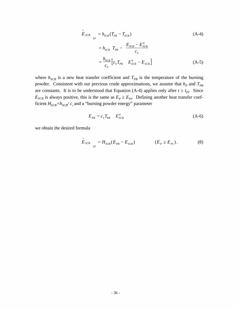
We now develop an equation for the heat transfer back into the SCB along thelines of that used to go from Eq. (6) to Eq. (7). The first step is to write the transfer rateas
- 36 -
E h T TSCBTF
SCB PB SCB
•
= −( ) (A-4)
= −−
h T
E EcSCB PB
SCB SCB
S
0
[ ]= + −hc
c T E ESCB
SS PB SCB SCB
0 (A-5)
where hSCB is a new heat transfer coefficient and TPB is the temperature of the burningpowder. Consistent with our previous crude approximations, we assume that hP and TPB
are constants. It is to be understood that Equation (A-4) applies only after t ≥ tPI. Since
ESCB is always positive, this is the same as EP ≥ EPI. Defining another heat transfer coef-ficient HSCB=hSCB/ c
S and a “burning powder energy” parameter
E c T EPB S PB SCB= + 0 (A-6)
we obtain the desired formula
E H E ESCBTF
SCB PB SCB
•
= −( ) ( )E EP PI≥ . (8)
- 37 -
Appendix B
The following is a netlist of a PSpice subcircuit for the SCB model (an asterisk inthe first column denotes a comment in PSpice).
* This is the SCB model which implements both the nonlinear loss term and the thermal* feedback model. It is intended for use only for detonators using SCBs of type 3-2b1+* with BNCP explosive powder pressed into TO46/Brass shells at 25 kpsi.
* Aloss is the loss coefficient AL, deltal is the size of the loss function transition* region in Volts,V0l is the SCB voltage at the transition region, EpioHp= EPI / HP,* Hscb=HSCB, Epb=EPB.
* Vmon is just a current monitor. The SCB current I is I(Vmon).
Vmon 1 5 0
* V(101) is the energy ESCB contained within the SCB itself. It is obtained by combining* the sources and losses described below and integrating the result. (The sources and* losses are represented as current sources charging or discharging a unit capacitance.)
* Gpower is the electrical power VI delivered to the det leads. Some of this energy is* deposited in the semiconductor material (V(101)) and some is lost through Gloss.
* Gloss is thermal energy lost to the substrate, aluminum lands, explosive powder,* etc. via the AL fL(V) term in Equation (5). Note minus sign in front of Aloss denoting* loss.
* The third line in the formula for Gloss is the value of the loss function fL(V) for SCB* voltages between V0l-deltal and V0l+deltal. It is evaluated on a circular arc in* (f,V/V0l) space.
* Eabs is the absolute value of the voltage at the SCB input leads. A separate voltage* source is used to evaluate it only to avoid repetition of the term abs(V(1,2)) in Gloss.* Rabs is just a resistor to complete the circuit.
Eabs 202 0 Value=abs(V(1,2))Rabs 0 202 1.0T
* Gpwdr is the rate at which energy is fed back into the SCB by the powder (see* Equation (8). Note that V(201) is the integral of Gignit.
.[Most of the entries in the table are not shown in the interest of brevity. Note that a dif-ferent table was used for the thermal feedback model than was used for the lossy modelalone. This was due to differences in the R vs E behavior of the SCBs at different energylevels (see main text).]
1 Thiokol CorporationAtt: W. B. Greeg, Jr., M. Kramer
P.O. Box 241,55 Thiokol RoadElkton, MD 21922-0241
1 Quantic Industries, Inc.Att: K. Willis, M. Berrera
990 Commercial StreetSan Carlos, CA 94070-4084
- 41 -
1 Robert W. InghamTeledyne McCormic Selph3601 Union RoadP.O. Box 6Hollister, CA 95024-006
1 R. W. Davis, LLNL, L-281 1 R. S. Lee, LLNL, L-281
1 MS 0311 J. W. Hole, 2671 1 MS 0328 J. A. Wilder, 2674 1 MS 0457 J. S. Rottler, 2001 1 MS 0481 M. M. Harcourt, 2167 1 MS 0481 M. A. Rosenthal, 2167 1 MS 0481 D. L. Thomas, 2167 4 MS 0486 S. S. Kawka, 2123 1 MS 0525 C. W. Bogdan, 1252 1 MS 0525 M. F. Deveney, 1252 1 MS 0525 P. V. Plunkett, 1252 1 MS 0953 W. E. Alzheimer, 1500 1 MS 0985 J. H. Stichman, 260010 MS 1453 R. W. Bickes, Jr. 1553 1 MS 1453 F. H. Braaten, Jr., 1553 1 MS 1453 M. C. Grubelich, 1553 1 MS 1453 S. M. Harris, 1553 1 MS 1453 G. R. Peevy, 1553 1 MS 1454 D. E. Wackerbarth, 1553 1 MS 1454 L. L. Bonzon, 1554 1 MS 1454 W. W. Tarbell, 1554 1 MS 0328 J. H. Weinlein, 2674 1 MS 9004 M. E. John, 8100 3 MS 9202 R. L. Bierbaum, 8116 1 MS 9202 H.-T. Chang, 8116 1 MS 9202 C. M. Furnberg, 811620 MS 9202 K. D. Marx, 8116 1 MS 9202 D. S. Post, 8116 1 MS 9202 J. F. Stamps, 8116 1 MS 9101 R. I. Eastin, 8411 1 MS 9101 K. R. Hughes, 8411 3 MS 9106 R. E. Oetken, 8417 1 MS 9106 J. L. Van De Vreugde, 8417
- 42 -
10 MS 9021 Technical Communications Department, 8815, for OSTI 1 MS 9021 Technical Communications Department, 8815/Technical
Library, MS 0899, 4414 4 MS 0899 Technical Library, 4414 3 MS 9018 Central Technical Files, 8940-2