Argonne National Laboratory, Argonne, Illinois 60439 operated by The University of Chicago for the United States Department of Energy under Contract W-31-109-Eng-38 Chemical Technology Division Chemical Technology Division Chemical Technology Division Chemical Technology Division Chemical Technology Division Chemical Technology Division Chemical Technology Division Chemical Technology Division Chemical Technology Division Chemical Technology Division Chemical Technology Division Chemical Technology Division Chemical Technology Division Chemical Technology Division Chemical Technology Division Chemical Technology Division Chemical Technology Division Chemical Technology Division Chemical Technology Division Chemical Technology Division Chemical Technology Division ANL-02/08 Characterization and Recovery of Solvent Entrained During the Use of Centrifugal Contactors by H. A. Arafat, M. C. Hash, A. S. Hebden, and R. A. Leonard
Transcript
Argonne National Laboratory, Argonne, Illinois 60439operated by The University of Chicagofor the United States Department of Energy under Contract W-31-109-Eng-38
Chemical TechnologyDivision
Chemical Technology Division
Chemical Technology Division
Chemical Technology Division
Chemical Technology Division
Chemical Technology Division
Chemical Technology Division
Chemical Technology Division
Chemical Technology Division
Chemical Technology Division
Chemical Technology Division
Chemical Technology Division
Chemical Technology Division
Chemical Technology Division
Chemical Technology Division
Chemical Technology Division
Chemical Technology Division
Chemical Technology Division
Chemical Technology Division
Chemical Technology Division
Chemical Technology Division
ANL-02/08
Characterization and Recoveryof Solvent Entrained During the
Use of Centrifugal Contactors
by H. A. Arafat, M. C. Hash,A. S. Hebden, and R. A. Leonard
Argonne National Laboratory, with facilities in the states of Illinois and Idaho, is ownedby the United States Government and operated by The University of Chicago under theprovisions of a contract with the Department of Energy.
DISCLAIMER
This report was prepared as an account of work sponsored by an agency ofthe United States Government. Neither the United States Government norany agency thereof, nor The University of Chicago, nor any of theiremployees or officers, makes any warranty, express or implied, or assumesany legal liability or responsibility for the accuracy, completeness, orusefulness of any information, apparatus, product, or process disclosed, orrepresents that its use would not infringe privately owned rights. Referenceherein to any specific commercial product, process, or service by trade name,trademark, manufacturer, or otherwise, does not necessarily constitute orimply its endorsement, recommendation, or favoring by the United StatesGovernment or any agency thereof. The views and opinions of documentauthors expressed herein do not necessarily state or reflect those of theUnited States Government or any agency thereof, Argonne NationalLaboratory, or The University of Chicago.
Available electronically at http://www.doe.gov/bridge
Available for a processing fee to U.S. Department ofEnergy and its contractors, in paper, from:
U.S. Department of EnergyOffice of Scientific and Technical InformationP.O. Box 62Oak Ridge, TN 37831-0062phone: (865) 576-8401fax: (865) 576-5728email: [email protected]
ANL-02/08
ARGONNE NATIONAL LABORATORY9700 South Cass Avenue
Argonne, IL 60439
CHARACTERIZATION AND RECOVERY OF SOLVENTENTRAINED DURING THE USE OF CENTRIFUGAL
CONTACTORS
by
H. A. Arafat, M. C. Hash, A. S. Hebden, and R. A. Leonard
APPENDIX B. CUMULATIVE DROPLET SIZE DISTRIBUTION DATA........................ 17
APPENDIX C. CALCULATIONS FOR SOLVENT RECOVERY IN A CSSXPILOT-PLANT DECANTER TANK............................................................ 20
iv
LIST OF FIGURES
No. Title Page
1. Flowsheet for the Proposed CSSX Process Pilot Plant at SRS........................................... 2
2. Experimental 4-cm Contactor Used for Decanter Tests...................................................... 4
3. Schematic of the Experimental Setup for the Decanter Tests............................................. 6
4. Size Distribution of Organic Droplets Entrained in Aqueous Effluents ............................. 9
LIST OF TABLES
No. Title Page
1. Mixing Intensity for Different Rotor Sizes ......................................................................... 5
2. Summary of Entrainment Measurement Tests .................................................................... 7
3. Average Droplet Size in Raffinate and Strip Effluents ..................................................... 10
A-1. Measurement of Control Samples by ORNL Using the Non-Modified Technique.......... 14
A-2. Measurements of Control Samples by ORNL Using the Modified Technique ................ 15
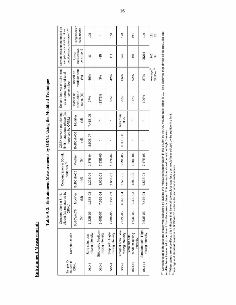
A-3. Entrainment Measurements by ORNL Using the Modified Technique............................ 16
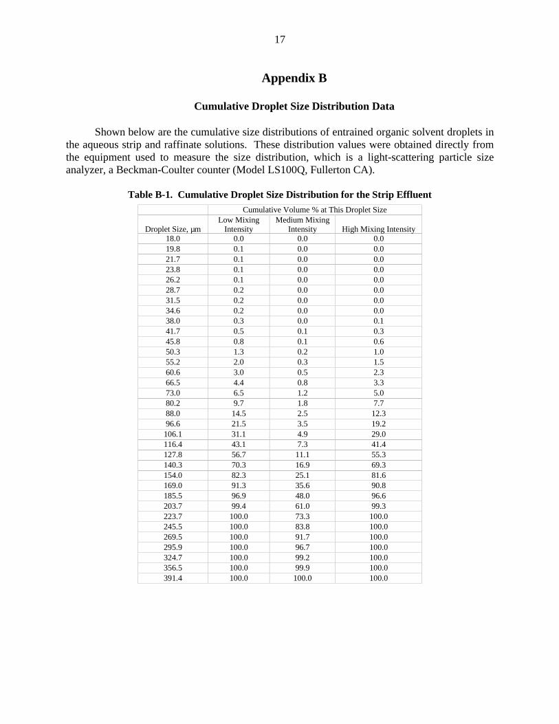
B-1. Cumulative Droplet Size Distribution for the Strip Effluent ............................................ 17
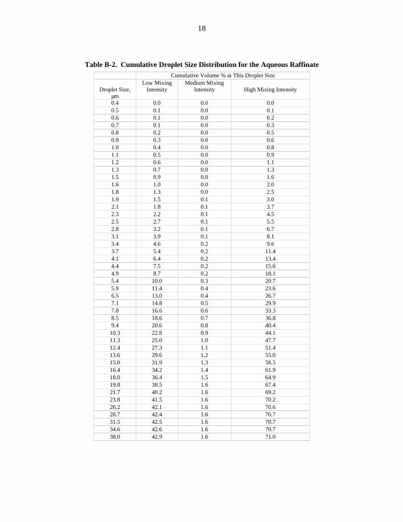
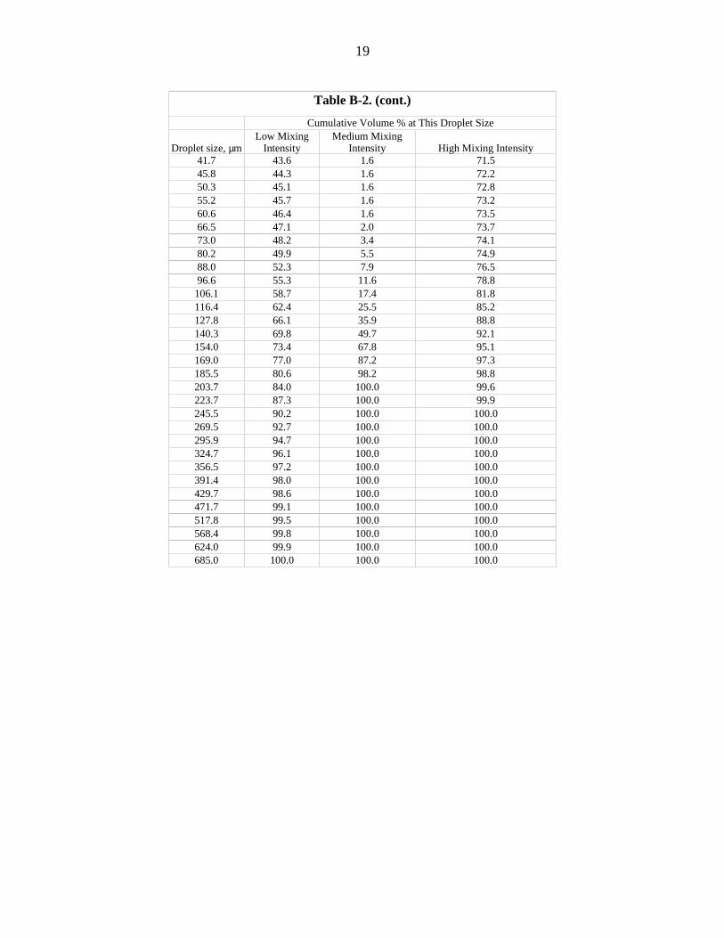
B-2. Cumulative Droplet Size Distribution for the Aqueous Raffinate .................................... 18
CHARACTERIZATION AND RECOVERY OF SOLVENT ENTRAINED DURING THEUSE OF CENTRIFUGAL CONTACTORS
by
H. A. Arafat, M. C. Hash, A. S. Hebden, and R. A. Leonard
October 31, 2001
ABSTRACT
In this work, we determined how a decanter for the aqueous effluents would work forsolvent extraction operations using a centrifugal contactor. Solvent entrainment was measured inthe raffinate and strip aqueous effluents in the caustic-side solvent extraction (CSSX) process.Values were obtained for both the solvent concentration and its droplet size distribution. Themixing intensity of the two phases in the mixing zone of the contactor was used to simulate theperformance of lab-scale, pilot-plant, and plant-scale contactors. The droplet size distributionswere used to estimate the amount of solvent that would be recovered using a decanter tank. Itwas concluded that the performance of decanter tanks will not be as effective in solvent recoveryin the CSSX plan as that of other equipment, such as centrifuges and coalescers. Future testingis recommended to verify the performance of this alternative equipment.
I. INTRODUCTION
About 34 million gallons of high-level radioactive waste are currently stored inunderground tanks at the Savannah River Site (SRS) in Aiken, South Carolina [LEVENSON-2000]. Recently, a process developed at Oak Ridge National Laboratory (ORNL), incollaboration with Argonne National Laboratory (ANL) and SRS, was selected to removecesium-137 (137Cs) from the waste prior to immobilizing the waste in low-level grout. Thetreatment technology, which is a caustic-side solvent extraction (CSSX) process, will utilize amultistage centrifugal contactor to extract 137Cs from the waste [LEONARD-2000]. The solventused in this process consists of four components: (1) an extractant, calix[4]arene-bis(tert-octylbenzo-crown-6), designated BoBCalixC6, which is a calixarene crown that is very specificfor cesium extraction, (2) a modifier, 1-(2,2,3,3, -tetrafluoropropoxy)-3-(4-sec-butylphenoxy)-2-propanol, also called Cs-7SB, which is an alkyl aryl polyether that keeps the extractant dissolvedin the solvent and increases its ability to extract cesium in the extraction section, (3) asuppressant, trioctylamine (TOA), which suppresses effects from organic impurities to ensurethat the cesium can be back-extracted from the solvent in the strip section, and (4) a diluent,Isopar®L, which is a mixture of branched hydrocarbons. The baseline solvent composition is0.01 M BoBCalixC6, 0.5 M Cs-7SB, and 0.001 M TOA in Isopar®L and is designated the"CSSX solvent."
1
2
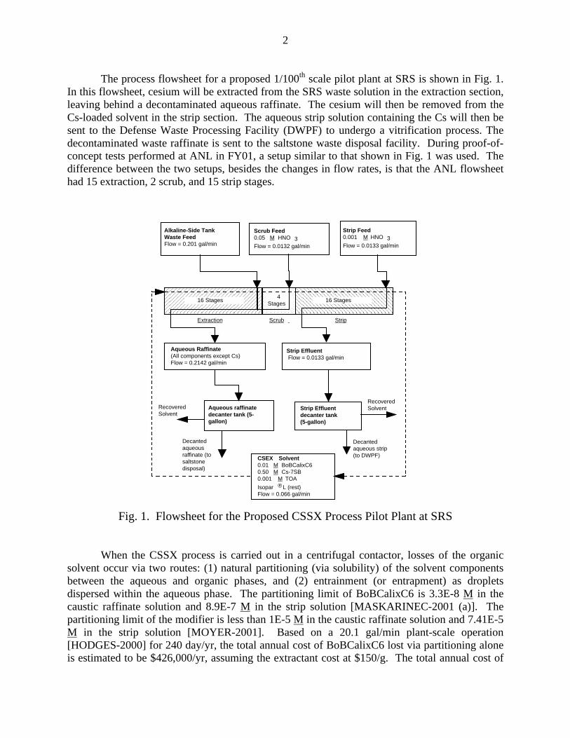
The process flowsheet for a proposed 1/100th scale pilot plant at SRS is shown in Fig. 1.In this flowsheet, cesium will be extracted from the SRS waste solution in the extraction section,leaving behind a decontaminated aqueous raffinate. The cesium will then be removed from theCs-loaded solvent in the strip section. The aqueous strip solution containing the Cs will then besent to the Defense Waste Processing Facility (DWPF) to undergo a vitrification process. Thedecontaminated waste raffinate is sent to the saltstone waste disposal facility. During proof-of-concept tests performed at ANL in FY01, a setup similar to that shown in Fig. 1 was used. Thedifference between the two setups, besides the changes in flow rates, is that the ANL flowsheethad 15 extraction, 2 scrub, and 15 strip stages.
Fig. 1. Flowsheet for the Proposed CSSX Process Pilot Plant at SRS
When the CSSX process is carried out in a centrifugal contactor, losses of the organicsolvent occur via two routes: (1) natural partitioning (via solubility) of the solvent componentsbetween the aqueous and organic phases, and (2) entrainment (or entrapment) as dropletsdispersed within the aqueous phase. The partitioning limit of BoBCalixC6 is 3.3E-8 M in thecaustic raffinate solution and 8.9E-7 M in the strip solution [MASKARINEC-2001 (a)]. Thepartitioning limit of the modifier is less than 1E-5 M in the caustic raffinate solution and 7.41E-5M in the strip solution [MOYER-2001]. Based on a 20.1 gal/min plant-scale operation[HODGES-2000] for 240 day/yr, the total annual cost of BoBCalixC6 lost via partitioning aloneis estimated to be $426,000/yr, assuming the extractant cost at $150/g. The total annual cost of
3
modifier lost via partitioning is estimated to be $207,000/yr for plant-scale operation. This cost isbased on modifier cost of $1.5/g, which is the projected commercial-production market value[BONNESEN-2001]. Thus, the total annual cost of BoBCalixC6 and modifier lost viapartitioning is about $0.6 M/yr. The amount of solvent lost as entrainment depends on the plantoperation, including process upsets that could cause this loss to increase. Using a decanter tank,for example, will help recover part of the entrained solvent, although it cannot recover anydissolved solvent. It was expected that the amount of solvent lost via entrainment would bemuch larger than that lost via solubility. Therefore, solvent recovery efforts here are focused onminimizing entrainment as the primary route for reducing solvent loss.
Due to the vigorous mixing of the aqueous and organic phases within the contactor unit,droplets of the solvent become entrained in the aqueous phase exiting the contactors. Suchentrainment has been observed during proof-of-concept tests at ANL. Similarly, SRS hasobserved some entrainment, ranging mainly from 0.01 to 0.4% and not exceeding 1%, during thereal-waste test performed there [CAMPBELL-2001]. Solvent entrainment occurs both in thestrip effluent and the decontaminated raffinate. It is desirable to recover the entrained solventfrom both aqueous flows for two reasons: (1) to maintain the organic contents of the aqueouseffluents within the limits set for the DWPF and the saltstone disposal facilities, and (2) toreduce the cost of the CSSX process by recovering the solvent. The current estimate of solventcost for the CSSX process is about $1900/L; 87% of this cost is attributed to the extractant,BoBCalixC6, and 13% is attributed to the modifier, Cs-7SB. A number of options are beingevaluated for the recovery of the entrained solvent. One of these options is to use settling(decanting) tanks. The pilot-plant flowsheet in Fig. 1 shows two 5-gallon decanter tanks, one foreach aqueous effluent. The amount of the organic phase separated in a decanter tank depends onthe size distribution of the dispersed (entrained) organic droplets, decanter size and geometry,and the total volume of entrained solvent. In the current work, we determined the droplet sizedistribution as well as the total volume of the entrained solvent.
II. EXPERIMENTAL
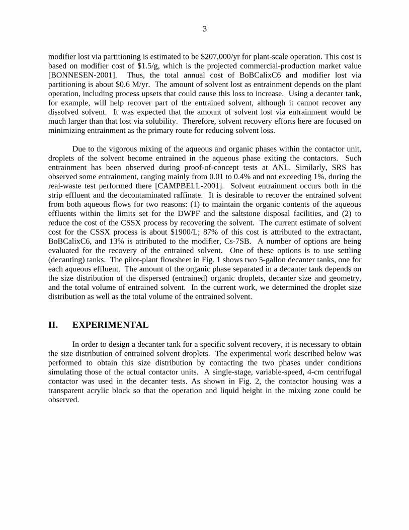
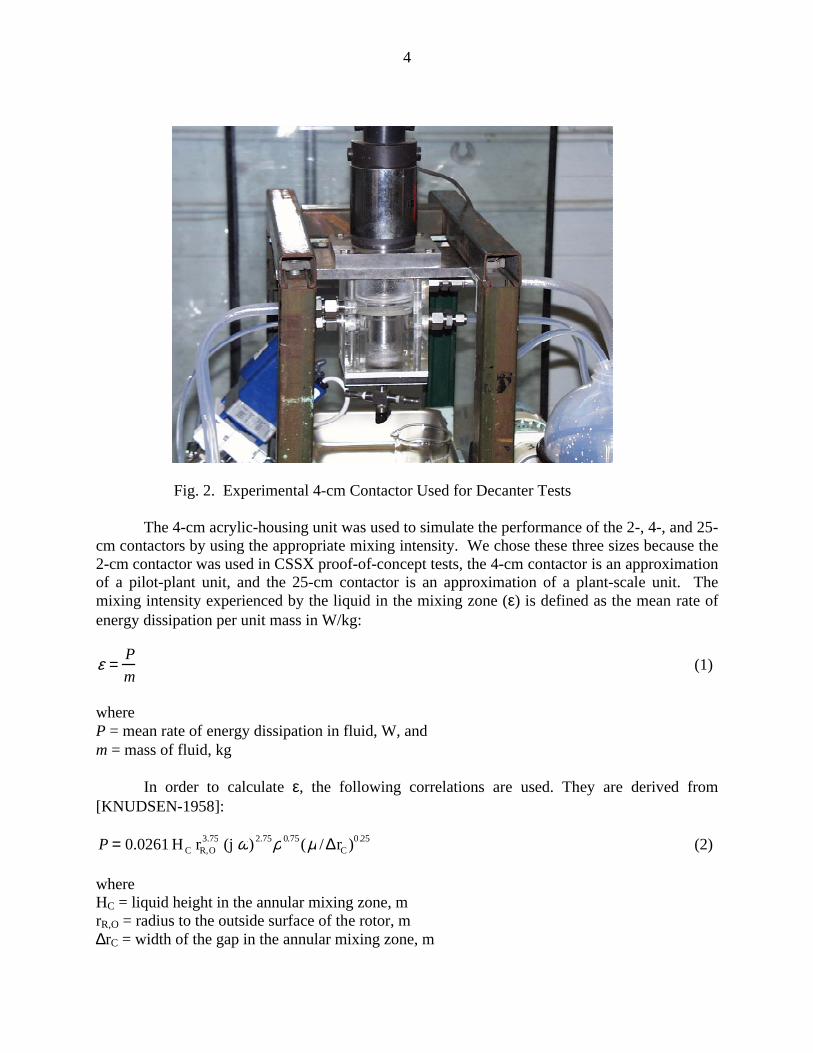
In order to design a decanter tank for a specific solvent recovery, it is necessary to obtainthe size distribution of entrained solvent droplets. The experimental work described below wasperformed to obtain this size distribution by contacting the two phases under conditionssimulating those of the actual contactor units. A single-stage, variable-speed, 4-cm centrifugalcontactor was used in the decanter tests. As shown in Fig. 2, the contactor housing was atransparent acrylic block so that the operation and liquid height in the mixing zone could beobserved.
4
Fig. 2. Experimental 4-cm Contactor Used for Decanter Tests
The 4-cm acrylic-housing unit was used to simulate the performance of the 2-, 4-, and 25-cm contactors by using the appropriate mixing intensity. We chose these three sizes because the2-cm contactor was used in CSSX proof-of-concept tests, the 4-cm contactor is an approximationof a pilot-plant unit, and the 25-cm contactor is an approximation of a plant-scale unit. Themixing intensity experienced by the liquid in the mixing zone (ε) is defined as the mean rate ofenergy dissipation per unit mass in W/kg:
ε =P
m(1)
whereP = mean rate of energy dissipation in fluid, W, andm = mass of fluid, kg
In order to calculate ε, the following correlations are used. They are derived from[KNUDSEN-1958]:
P = 0.0261 H C rR,O3.75 (j ω)2.75ρ 0.75(µ /∆rC )0.25 (2)
whereHC = liquid height in the annular mixing zone, mrR,O = radius to the outside surface of the rotor, m∆rC = width of the gap in the annular mixing zone, m
5
µ = viscosity of the bulk liquid or continuous phase of the dispersion, Pa•sρ = fluid or dispersion density, kg/m3
ω = angular velocity of the rotor, rad/s, andj = 0.0554 (log NRe)+ 1.368, 3x10³ < NRe < 1x10⁶
where NRe is the Reynolds number, defined as
NRe = 2jρω rR,O∆rC/µ (3)
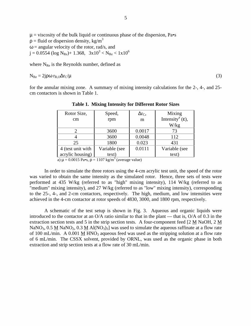
for the annular mixing zone. A summary of mixing intensity calculations for the 2-, 4-, and 25-cm contactors is shown in Table 1.
Table 1. Mixing Intensity for Different Rotor Sizes
In order to simulate the three rotors using the 4-cm acrylic test unit, the speed of the rotorwas varied to obtain the same intensity as the simulated rotor. Hence, three sets of tests wereperformed at 435 W/kg (referred to as "high" mixing intensity), 114 W/kg (referred to as"medium" mixing intensity), and 27 W/kg (referred to as "low" mixing intensity), correspondingto the 25-, 4-, and 2-cm contactors, respectively. The high, medium, and low intensities wereachieved in the 4-cm contactor at rotor speeds of 4830, 3000, and 1800 rpm, respectively.
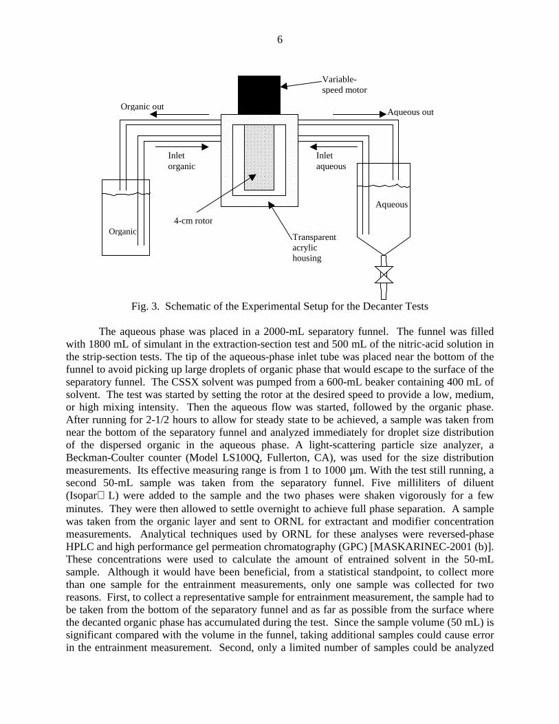
A schematic of the test setup is shown in Fig. 3. Aqueous and organic liquids wereintroduced to the contactor at an O/A ratio similar to that in the plant — that is, O/A of 0.3 in theextraction section tests and 5 in the strip section tests. A four-component feed [2 M NaOH, 2 MNaNO3, 0.5 M NaNO2, 0.3 M Al(NO3)3] was used to simulate the aqueous raffinate at a flow rateof 100 mL/min. A 0.001 M HNO3 aqueous feed was used as the stripping solution at a flow rateof 6 mL/min. The CSSX solvent, provided by ORNL, was used as the organic phase in bothextraction and strip section tests at a flow rate of 30 mL/min.
6
Variable-speed motor
Inletaqueous
Aqueous out
Inletorganic
Organic out
Aqueous
OrganicTransparentacrylichousing
4-cm rotor
Fig. 3. Schematic of the Experimental Setup for the Decanter Tests
The aqueous phase was placed in a 2000-mL separatory funnel. The funnel was filledwith 1800 mL of simulant in the extraction-section test and 500 mL of the nitric-acid solution inthe strip-section tests. The tip of the aqueous-phase inlet tube was placed near the bottom of thefunnel to avoid picking up large droplets of organic phase that would escape to the surface of theseparatory funnel. The CSSX solvent was pumped from a 600-mL beaker containing 400 mL ofsolvent. The test was started by setting the rotor at the desired speed to provide a low, medium,or high mixing intensity. Then the aqueous flow was started, followed by the organic phase.After running for 2-1/2 hours to allow for steady state to be achieved, a sample was taken fromnear the bottom of the separatory funnel and analyzed immediately for droplet size distributionof the dispersed organic in the aqueous phase. A light-scattering particle size analyzer, aBeckman-Coulter counter (Model LS100Q, Fullerton, CA), was used for the size distributionmeasurements. Its effective measuring range is from 1 to 1000 µm. With the test still running, asecond 50-mL sample was taken from the separatory funnel. Five milliliters of diluent(Isopar L) were added to the sample and the two phases were shaken vigorously for a fewminutes. They were then allowed to settle overnight to achieve full phase separation. A samplewas taken from the organic layer and sent to ORNL for extractant and modifier concentrationmeasurements. Analytical techniques used by ORNL for these analyses were reversed-phaseHPLC and high performance gel permeation chromatography (GPC) [MASKARINEC-2001 (b)].These concentrations were used to calculate the amount of entrained solvent in the 50-mLsample. Although it would have been beneficial, from a statistical standpoint, to collect morethan one sample for the entrainment measurements, only one sample was collected for tworeasons. First, to collect a representative sample for entrainment measurement, the sample had tobe taken from the bottom of the separatory funnel and as far as possible from the surface wherethe decanted organic phase has accumulated during the test. Since the sample volume (50 mL) issignificant compared with the volume in the funnel, taking additional samples could cause errorin the entrainment measurement. Second, only a limited number of samples could be analyzed
7
within the budget allocated for ORNL to perform the analyses.
III. RESULTS AND DISCUSSION
1. Entrainment Measurements
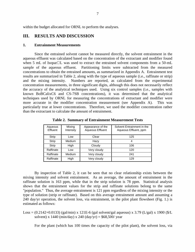
Since the entrained solvent cannot be measured directly, the solvent entrainment in theaqueous effluent was calculated based on the concentration of the extractant and modifier foundwhen 5 mL of Isopar L was used to extract the entrained solvent components from a 50-mLsample of the aqueous effluent. Partitioning limits were subtracted from the measuredconcentrations to obtain the entrained amounts, as summarized in Appendix A. Entrainment testresults are summarized in Table 2, along with the type of aqueous sample (i.e., raffinate or strip)and the mixing intensity. Numbers are reported, as calculated from the experimentalconcentration measurements, in three significant digits, although this does not necessarily reflectthe accuracy of the analytical techniques used. Using six control samples (i.e., samples withknown BoBCalixC6 and CS-7SB concentrations), it was determined that the analyticaltechniques used by ORNL for measuring the concentrations of extractant and modifier weremore accurate in the modifier concentration measurement (see Appendix A). This wasparticularly true at lower concentrations. Therefore, we used the modifier concentration ratherthan the extractant to calculate the amount of entrainment.
Table 2. Summary of Entrainment Measurement Tests
AqueousEffluent
MixingIntensity
Appearance of theAqueous Effluent
Solvent Entrainment in theAqueous Effluent, ppm
Strip Low Clear 125
Strip Medium Hazy 4
Strip High Cloudy 106
Raffinate Low Very cloudy 120
Raffinate Medium Very cloudy 241
Raffinate High Very cloudy 129
By inspection of Table 2, it can be seen that no clear relationship exists between themixing intensity and solvent entrainment. As an average, the amount of entrainment in theraffinate solution is 163 ppm, while that in the strip solution is 78 ppm. Statistical analysisshows that the entrainment values for the strip and raffinate solutions belong to the same"population." Thus, the average entrainment is 121 ppm regardless of the mixing intensity or thetype of solution (strip or raffinate). Based on this average entrainment amount and assuming a240 day/yr operation, the solvent loss, via entrainment, in the pilot plant flowsheet (Fig. 1.) isestimated as follows:
Loss = (0.2142+0.0133) (gal/min) x 121E-6 (gal solvent/gal aqueous) x 3.79 (L/gal) x 1900 ($/Lsolvent) x 1440 (min/day) x 240 (day/yr) = $68,500/ year
For the plant (which has 100 times the capacity of the pilot plant), the solvent loss, via
8
entrainment, would be about $7M/yr if no solvent recovery action was taken. This indicates that,particularly for the plant operation, there could be large cost benefit if most of the entrainedsolvent is recovered and recycled. Note that the annual cost of solvent lost via entrainment isabout 11 times the cost of solvent lost via partitioning ($0.6M/yr), as calculated earlier.
Also noted in Table 2 is the appearance of the aqueous phase in the separatory funnel atthe time when the sample was taken. These observations show no clear relationship between thelevel of cloudiness of the aqueous phase and the amount of solvent entrained in it. However, itwas noticed that solution cloudiness increased with mixing intensity and was always higher forthe simulant than for the strip solution. There are two possible explanations for this observation.First, submicron size droplets that cannot be effectively accounted for using the Coulter counter(detection limit about 1 µm) might contribute significantly to the level of cloudiness observed inthe aqueous phase. Second, entrained air bubbles, caused by the high mixing intensity, might beresponsible for the cloudy appearance of the solution. Both reasons would explain the increasein cloudiness with mixing intensity (Table 2). In any case, cloudiness should not be used toestimate the level of solvent entrainment.
2. Droplet Size Distribution of Entrained Solvent
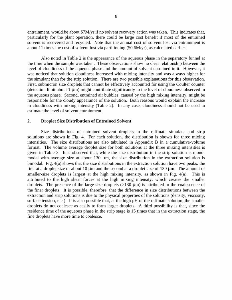
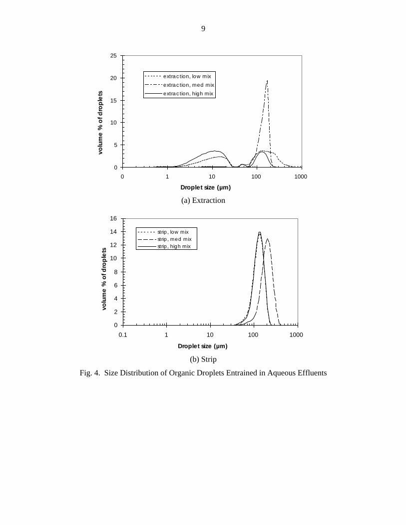
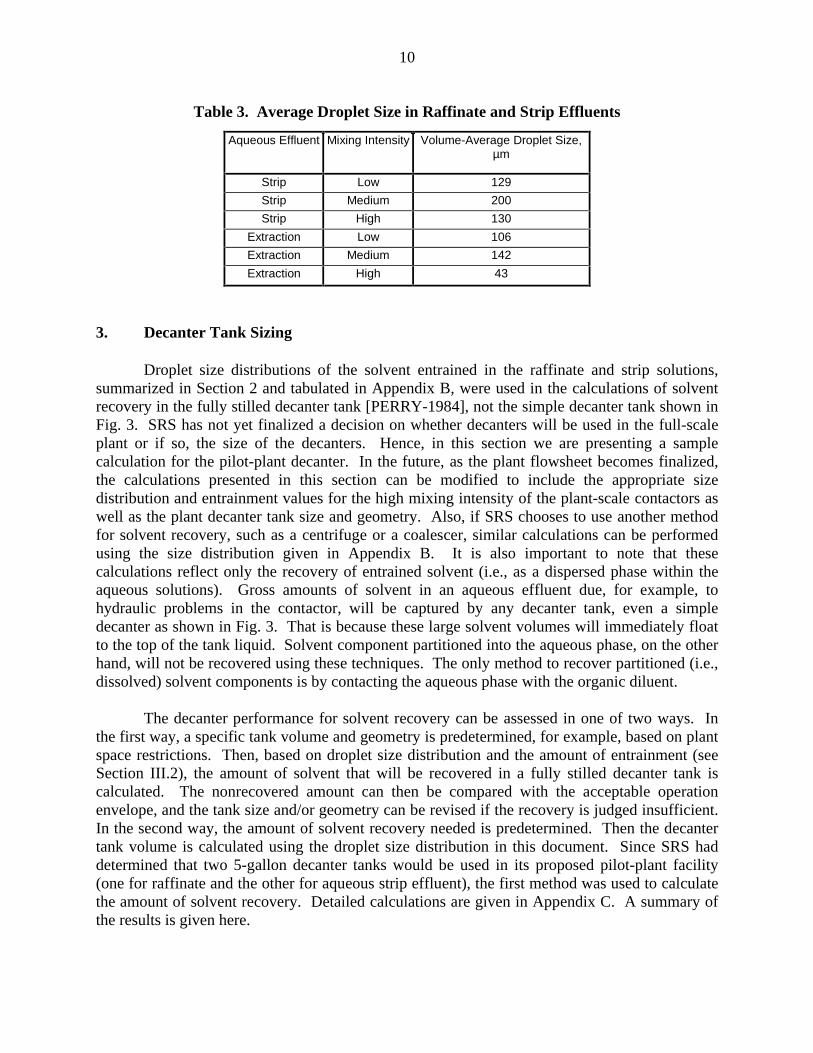
Size distributions of entrained solvent droplets in the raffinate simulant and stripsolutions are shown in Fig. 4. For each solution, the distribution is shown for three mixingintensities. The size distributions are also tabulated in Appendix B in a cumulative-volumeformat. The volume average droplet size for both solutions at the three mixing intensities isgiven in Table 3. It is observed that, while the size distribution in the strip solution is mono-modal with average size at about 130 µm, the size distribution in the extraction solution isbimodal. Fig. 4(a) shows that the size distributions in the extraction solution have two peaks: thefirst at a droplet size of about 10 µm and the second at a droplet size of 130 µm. The amount ofsmaller-size droplets is largest at the high mixing intensity, as shown in Fig. 4(a). This isattributed to the high shear forces at the high mixing intensity, which creates the smallerdroplets. The presence of the large-size droplets (>130 µm) is attributed to the coalescence ofthe finer droplets. It is possible, therefore, that the difference in size distributions between theextraction and strip solutions is due to the physical properties of the solutions (density, viscosity,surface tension, etc.). It is also possible that, at the high pH of the raffinate solution, the smallerdroplets do not coalesce as easily to form larger droplets. A third possibility is that, since theresidence time of the aqueous phase in the strip stage is 15 times that in the extraction stage, thefine droplets have more time to coalesce.
9
0
5
10
15
20
25
0 1 10 100 1000
Droplet size (µm)
volu
me
% o
f dro
ple
ts
extraction, low mix
extraction, med mix
extraction, high mix
(a) Extraction
0
2
4
6
8
10
12
14
16
0.1 1 10 100 1000
Droplet size (µm)
volu
me
% o
f dro
ple
ts
strip, low mixstrip, med mixstrip, high mix
(b) Strip
Fig. 4. Size Distribution of Organic Droplets Entrained in Aqueous Effluents
10
Table 3. Average Droplet Size in Raffinate and Strip Effluents
Droplet size distributions of the solvent entrained in the raffinate and strip solutions,summarized in Section 2 and tabulated in Appendix B, were used in the calculations of solventrecovery in the fully stilled decanter tank [PERRY-1984], not the simple decanter tank shown inFig. 3. SRS has not yet finalized a decision on whether decanters will be used in the full-scaleplant or if so, the size of the decanters. Hence, in this section we are presenting a samplecalculation for the pilot-plant decanter. In the future, as the plant flowsheet becomes finalized,the calculations presented in this section can be modified to include the appropriate sizedistribution and entrainment values for the high mixing intensity of the plant-scale contactors aswell as the plant decanter tank size and geometry. Also, if SRS chooses to use another methodfor solvent recovery, such as a centrifuge or a coalescer, similar calculations can be performedusing the size distribution given in Appendix B. It is also important to note that thesecalculations reflect only the recovery of entrained solvent (i.e., as a dispersed phase within theaqueous solutions). Gross amounts of solvent in an aqueous effluent due, for example, tohydraulic problems in the contactor, will be captured by any decanter tank, even a simpledecanter as shown in Fig. 3. That is because these large solvent volumes will immediately floatto the top of the tank liquid. Solvent component partitioned into the aqueous phase, on the otherhand, will not be recovered using these techniques. The only method to recover partitioned (i.e.,dissolved) solvent components is by contacting the aqueous phase with the organic diluent.
The decanter performance for solvent recovery can be assessed in one of two ways. Inthe first way, a specific tank volume and geometry is predetermined, for example, based on plantspace restrictions. Then, based on droplet size distribution and the amount of entrainment (seeSection III.2), the amount of solvent that will be recovered in a fully stilled decanter tank iscalculated. The nonrecovered amount can then be compared with the acceptable operationenvelope, and the tank size and/or geometry can be revised if the recovery is judged insufficient.In the second way, the amount of solvent recovery needed is predetermined. Then the decantertank volume is calculated using the droplet size distribution in this document. Since SRS haddetermined that two 5-gallon decanter tanks would be used in its proposed pilot-plant facility(one for raffinate and the other for aqueous strip effluent), the first method was used to calculatethe amount of solvent recovery. Detailed calculations are given in Appendix C. A summary ofthe results is given here.
11
Calculations in Appendix C show that, by using two standing cylindrical 5-gal decantertanks (80% full with liquid height equal to tank diameter) for the two aqueous effluents in aCSSX plant, recovery of the entrained solvent will be 98% in the raffinate solution and nearly100% in the strip solution. Although this is a very good recovery rate for the pilot plant, usingdecanter tanks might not be a suitable recovery option for the final treatment plant for thefollowing reasons:
• In the treatment plant, a very large decanter tank will be needed to achieve anacceptable rate of solvent recovery from the raffinate. For example, at a feed flow rateof 20.1 gal/min and assuming a cylindrical tank with a geometry similar to that of thepilot plant, a 3125-gallon tank (diameter = 2.3 m, height =2.9 m) can achieve only29% solvent recovery. To achieve higher recovery values, a much larger tank will beneeded.
• In decanter tanks, a proper tank operation requires feeding the liquid to the tank at theinterphase zone [PERRY-1984] to ensure minimum liquid disturbances. At anaverage of 121 ppm organic-in-aqueous carryover, the organic phase will be minimalcompared with the aqueous phase, which makes feeding at the interphase zone hard toachieve. For the same reason, continuous removal of recovered solvent from the tankmight be impractical.
To overcome these obstacles facing the use of decanter tanks in the plant facility, werecommend evaluating one of the following two alternatives:
• Coalescers: In a coalescer, small drops of a fine dispersion are caused to coalesce andthus become large and more readily separable from the bulk liquid. Coalescerscontain mats, beds, or layers of porous or fibrous solids whose properties areespecially designed to attract the fine organic droplets, which then collide on thesesurfaces and form larger droplets. Coalescers are particularly suitable for solventrecovery from the raffinate since (1) the amount of solvent entrained is minimal withrespect to the aqueous volume, and (2) a significant portion of the droplets entrained inthe raffinate are between 1 and 50 µm. Using a coalescer will increase the percentageof the larger droplets, facilitating their separation.
• Centrifuge: By utilizing the high g-force of the centrifuge, enhanced phase separationcan be achieved and most of the smaller-sized droplets, which are not recovered in agravity-settling decanter, can be recovered. Commercial centrifuges are available incompact sizes that can process the aqueous effluents in the plant in a continuousfashion.
Although further testing is needed to verify the efficiency of these two alternatives, webelieve that using either one of them will provide significant enhancement over the decantertank, especially for solvent recovery from the aqueous raffinate solution since its flow rate is 16times that of the aqueous strip effluent.
12
IV. SUMMARY AND CONCLUSIONS
Two sets of tests were performed to simulate the performance of the extraction and stripsections of the contactors in the CSSX process. Each set included tests at low, medium, and highmixing intensity in a single-stage, 4-cm centrifugal contactor. The low-intensity tests simulatethe performance of 2-cm (lab-scale) contactors, the medium-intensity tests simulate 4-cm (pilot-scale) contactor, and the high-intensity tests simulate 25-cm (full-scale) contactors. During eachtest, the volume of solvent entrained in the aqueous effluent and the size distribution of theentrained solvent droplets were measured. The average droplet size for the extraction sectionwas 163 ppm, while that for the strip section was 78 ppm. However, these differences are notstatistically significant and an average volume of entrained solvent of 121 ppm was used for allcases. The size distributions for the entrained solvent were also measured. We found moresmall droplets in the aqueous raffinate from the extraction section than in the aqueous stripeffluent.
The droplet size distributions obtained here were used to estimate the amount of solventrecovery achievable in the planned 5-gallon pilot-plant decanter tanks if they are totally stilled.Assuming a cylindrical tank with liquid height equal to tank diameter, the calculations showedthat high solvent recovery (>98%) is achievable. However, calculations showed that for the finaltreatment plant, a 3100-gallon decanter tank will be needed to achieve a moderate 30% solventrecovery from the raffinate effluent. To improve the recovery rate in the plant facility and toovercome other technical difficulties associated with decanter tanks, further testing is neededother means of solvent recovery such as coalescers or centrifuges.
V. ACKNOWLEDGMENTS
The authors are grateful for helpful discussions with Mike Maskarinec, Latitia Delmau,and Bruce Moyer from Oak Ridge National Laboratory. This work was supported by the U.S.Department of Energy, Office of Environmental Management, through (1) the Office of ProjectCompletion and (2) the Tank Focus Area of the Office of Science and Technology underContract W-31-109-Eng-38.
13
REFERENCES
BONNESEN-2001P. V. Bonnesen, Oak Ridge National Laboratory, private communication (2001).
CAMPBELL-2001S. G. Campbell, M. W. Geeting, C. W. Kennell, J. D. Law, R. A. Leonard, M. A. Norato,R. A. Pierce, T. A. Todd, D. D. Walker, and W. R. Wilmarth, “Demonstration of Caustic-SideSolvent Extraction with Savannah River Site High Level Waste,” Westinghouse Savannah RiverCompany Report WSRC-TR-2001-00223 (2001).
HODGES-2000M. E. Hodges, “Design Input - Caustic Side Solvent Extraction Flowsheet - Proof of ConceptTesting,” Westinghouse Savannah River Company Report HLW-SDT-2000-000356 (2000).
KNUDSEN-1958J. G. Knudsen and D. L. Katz, Fluid Dynamics and Heat Transfer, McGraw-Hill, New York(1958).
LEVENSON-2000M. Levenson et al., "Alternatives for High-Level Waste Salt Processing at the Savannah RiverSite,” National Research Council, National Academy Press, Washington, D.C. (2000).
LEONARD-2000R. A. Leonard, S. B. Aase, H. A. Arafat, C. Conner, J. R. Falkenberg, and G. F. Vandegrift,“Proof-of-Concept Flowsheet Tests for Caustic-Side Solvent Extraction of Cesium from TankWaste,” Argonne National Laboratory Report ANL-00/30 (2000).
MASKARINEC-2001 (a)M. P. Maskarinec, Oak Ridge National Laboratory, unpublished data.
MASKARINEC-2001 (b)M. P. Maskarinec, J. E. Caton, and T. L. White, “Analytical Methods Development in Support ofthe Caustic Side Solvent Extraction System,” Oak Ridge National Laboratory ReportCERS/SR/SX/022 (2001).
MOYER-2001B. A. Moyer, P. V. Bonnesen, J. E. Caton, C. R. Duchemin, T. G. Levitskaia, F. V. Sloop,S. D. Alexandratos, G. M. Brown, L. H. Delmau, T. J. Haverlock, M. P. Maskarinec, and C. L.Stine, “Caustic-Side Solvent Extraction Chemical and Physical Properties: Progress in FY2000and FY2001,” Oak Ridge National Laboratory Report CERS/SR/SX/019, Rev. 0 (2001).
PERRY-1984R. H. Perry and D. Green, Perry’s Chemical Engineers’ Handbook, 6th edition, McGraw Hill,New York (1984).
14
Appendix A
Entrainment Calculation Data
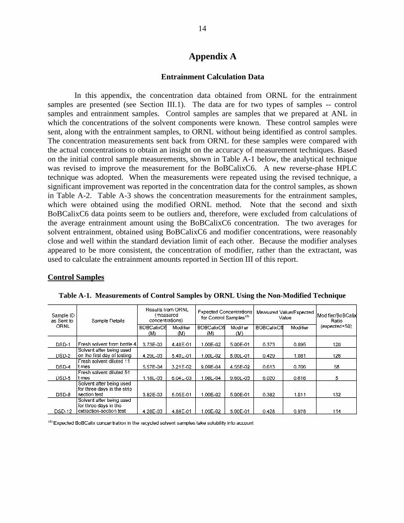
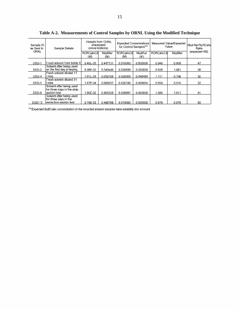
In this appendix, the concentration data obtained from ORNL for the entrainmentsamples are presented (see Section III.1). The data are for two types of samples -- controlsamples and entrainment samples. Control samples are samples that we prepared at ANL inwhich the concentrations of the solvent components were known. These control samples weresent, along with the entrainment samples, to ORNL without being identified as control samples.The concentration measurements sent back from ORNL for these samples were compared withthe actual concentrations to obtain an insight on the accuracy of measurement techniques. Basedon the initial control sample measurements, shown in Table A-1 below, the analytical techniquewas revised to improve the measurement for the BoBCalixC6. A new reverse-phase HPLCtechnique was adopted. When the measurements were repeated using the revised technique, asignificant improvement was reported in the concentration data for the control samples, as shownin Table A-2. Table A-3 shows the concentration measurements for the entrainment samples,which were obtained using the modified ORNL method. Note that the second and sixthBoBCalixC6 data points seem to be outliers and, therefore, were excluded from calculations ofthe average entrainment amount using the BoBCalixC6 concentration. The two averages forsolvent entrainment, obtained using BoBCalixC6 and modifier concentrations, were reasonablyclose and well within the standard deviation limit of each other. Because the modifier analysesappeared to be more consistent, the concentration of modifier, rather than the extractant, wasused to calculate the entrainment amounts reported in Section III of this report.
Control Samples
Table A-1. Measurements of Control Samples by ORNL Using the Non-Modified Technique
Shown below are the cumulative size distributions of entrained organic solvent droplets inthe aqueous strip and raffinate solutions. These distribution values were obtained directly fromthe equipment used to measure the size distribution, which is a light-scattering particle sizeanalyzer, a Beckman-Coulter counter (Model LS100Q, Fullerton CA).
Table B-1. Cumulative Droplet Size Distribution for the Strip EffluentCumulative Volume % at This Droplet Size
Calculations for Solvent Recovery in a CSSX Pilot-Plant Decanter Tank
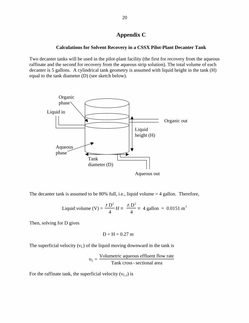
Two decanter tanks will be used in the pilot-plant facility (the first for recovery from the aqueousraffinate and the second for recovery from the aqueous strip solution). The total volume of eachdecanter is 5 gallons. A cylindrical tank geometry is assumed with liquid height in the tank (H)equal to the tank diameter (D) (see sketch below).
The decanter tank is assumed to be 80% full, i.e., liquid volume = 4 gallon. Therefore,
Liquid volume (V) = π D2
4H =
π D3
4= 4 gallon = 0.0151 m3
Then, solving for D gives
D = H = 0.27 m
The superficial velocity (vL) of the liquid moving downward in the tank is
vL = Volumetric aqueous effluent flow rate
Tank cross - sectional area
For the raffinate tank, the superficial velocity (vL,r) is
Aqueousphase
Organicphase
Liquidheight (H)
Tankdiameter (D)
Liquid in
Aqueous out
Organic out
21
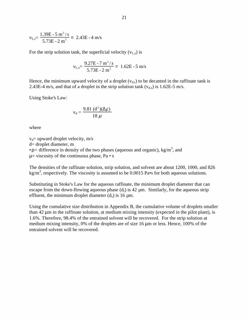
vL,r= 1.39E - 5 m3 / s
5.73E - 2 m2 = 2.43E - 4 m/s
For the strip solution tank, the superficial velocity (vL,s) is
vL,s= 9.27E - 7 m3 / s
5.73E - 2 m2 = 1.62E - 5 m/s
Hence, the minimum upward velocity of a droplet (vd,r) to be decanted in the raffinate tank is2.43E-4 m/s, and that of a droplet in the strip solution tank (vd,s) is 1.62E-5 m/s.
Using Stoke’s Law:
vd = 9.81 (d2 )(∆ρ)
18 µ
where
vd= upward droplet velocity, m/sd= droplet diameter, m•ρ= difference in density of the two phases (aqueous and organic), kg/m3, andµ= viscosity of the continuous phase, Pa • s
The densities of the raffinate solution, strip solution, and solvent are about 1200, 1000, and 826kg/m3, respectively. The viscosity is assumed to be 0.0015 Pa•s for both aqueous solutions.
Substituting in Stoke's Law for the aqueous raffinate, the minimum droplet diameter that canescape from the down-flowing aqueous phase (dr) is 42 µm. Similarly, for the aqueous stripeffluent, the minimum droplet diameter (ds) is 16 µm.
Using the cumulative size distribution in Appendix B, the cumulative volume of droplets smallerthan 42 µm in the raffinate solution, at medium mixing intensity (expected in the pilot plant), is1.6%. Therefore, 98.4% of the entrained solvent will be recovered. For the strip solution atmedium mixing intensity, 0% of the droplets are of size 16 µm or less. Hence, 100% of theentrained solvent will be recovered.
22
Distribution List for ANL-02/08
Internal (Printed and Electronic Copies):
S. B. AaseH. A. Arafat (5)A. J. BakelD. B. ChamberlainY. I. ChangM. L. DietzE. Freiberg
A. V. GuelisM. C. HashA. S. HebdenJ. E. HeltM. D. KaminskiR. A. Leonard (5)D. Lewis (2)
K. L. NashM. C. Regalbuto (5)M. J. SteindlerG. F. VandegriftS. K. Zussman
Internal (Electronic Copy Only):
D. L. BowersR. J. FinchE. C. GayC. J. MertzJ. SedletTIS Files
External (Printed and Electronic Copies):
Chemical Technology Division Review Committee Members:H. U. Anderson, University of Missouri-Rolla, Rolla, MOA. L. Bement, Jr., Purdue University, West Lafayette, INC. L. Hussey, University of Mississippi, University, MSM. V. Koch, University of Washington, Seattle, WAV. P. Roan, Jr., University of Florida, Gainesville, FLJ. R. Selman, Illinois Institute of Technology, Chicago, ILJ. S. Tulenko, University of Florida, Gainesville, FL
J. F. Birdwell, Oak Ridge National Laboratory, Oak Ridge, TNP. V. Bonnesen, Oak Ridge National Laboratory, Oak Ridge, TNS. G. Campbell, Westinghouse Savannah River Company, Aiken, SCJ. T. Carter, Westinghouse Savannah River Company, Aiken, SCC. Conner, Bolingbrook, ILL. H. Delmau, Oak Ridge National Laboratory, Oak Ridge, TNH. D. Harmon, Westinghouse Savannah River Company, Aiken, SCR. T. Jubin, Oak Ridge National Laboratory, Oak Ridge, TNJ. D. Law, Idaho National Engineering and Environmental Laboratory, Idaho Falls, IDR. Leugemors, Pacific Northwest National Laboratory, Richland, WAB. A. Moyer, Oak Ridge National Laboratory, Oak Ridge, TNM. Norato, Westinghouse Savannah River Company, Aiken, SCR. A. Pierce, Westinghouse Savannah River Company, Aiken, SCP. C. Suggs, DOE-SR, Aiken, South CarolinaM. C. Thompson, Westinghouse Savannah River Company, Aiken, SCT. A. Todd, INEEL, Idaho Falls, IDD. D. Walker, Westinghouse Savannah River Company, Aiken, SC
23
External (Printed Copy Only):
ANL-E-LibraryANL-W-LibraryTanks Focus Area Technical Team, c/o B. J. Williams, Pacific Northwest National Laboratory,Richland, WATanks Focus Area Field Lead, c/o T. P. Pietrok, Richland Operations Office, Richland, WATanks Focus Area Headquarters Program Manager, c/o, K. D. Gerdes, DOE-EM,Germantown, MD
External (Electronic Copy Only):
DOE-OSTIW. D. Clark, DOE-SR, Aiken, SCS. M. Dinehart, Los Alamos National Laboratory, Los Alamos, NMR. E. Edwards, Westinghouse Savannah River Company, Aiken, SCS. D. Fink, Westinghouse Savannah River Company, Aiken, SCL. N. Klatt, Oak Ridge National Laboratory, Oak Ridge, TND. E. Kurath, Battelle, Pacific Northwest National Laboratory, Richland, WAK. T. Lang, USDOE, Washington, DCJ. W. McCullough, USDOE, Aiken, SCC. P. McGinnis, Oak Ridge National Laboratory, Oak Ridge, TNA. L. Olson, Idaho National Engineering and Environmental Laboratory, Idaho Falls, IDM. J. Palmer, Los Alamos National Laboratory, Los Alamos, NML. M. Papouchado, Westinghouse Savannah River Company, Aiken, SCR. A. Peterson, Bechtel-Washington Process Technology, Richland, WAB. M. Rapko, Battelle, Pacific Northwest National Laboratory, Richland, WAR. D. Rogers, University of Alabama, Tuscaloosa, ALK. J. Rueter, Bechtel-Washington Process Technology, Richland, WAP. Rutland, Bechtel-Washington Process Technology, Richland, WAS. N. Schlahta, Battelle, Pacific Northwest National Laboratory, Richland, WAJ. L. Swanson, Richland, WAW. L. Tamosaitis, Westinghouse Savannah River Company, Aiken, SCL. L. Tavlarides, Syracuse University, Syracuse, NYD. W. Tedder, Georgia Institute of Technology, Atlanta, GAV. Van Brunt, University of South Carolina, Columbia, SCJ. F. Walker, Oak Ridge National Laboratory, Oak Ridge, TNJ. S. Watson, Oak Ridge National Laboratory, Oak Ridge, TNR. M. Wham, Oak Ridge National Laboratory, Oak Ridge, TNW. R. Wilmarth, Westinghouse Savannah River Company, Aiken, SC