The mixing properties of passive scalars in time-dependent flows depend very strongly on the chaotic nature of Lagrangian particle trajectories. The more rap-idly particles separate from each other, the more efficientmixing can be since a patch of tracer will be stretchedinto filaments of small width that will spread and mixthrough the entire fluid. The stretching process of a patchof tracer is equivalent to the growth of the tracer gradi-ent and ideas of dynamical systems can be applied. Herwe follow this approach and compare results fromLyapunov theory to results concerning the tracer gradi-ent dynamics in a two-dimensional turbulent flow.Lyapunov exponents were extensively used for this kindof problem but we stress here the importance ofLyapunov vectors. These vectors give information on thedifferent properties of stirring for finite times, such aslocal reversibility „or ‘‘chaoticity’’ … of the tracer gradientdynamics.
I. INTRODUCTION
An important property of two-dimensional timedependent flows is that Lagrangian particles can display cotic trajectories, even in the case of simple Eulerian velocfields. Close particles separate very quickly from each otand tracer patches spread rapidly to fill the entire charegion.1–5 This phenomenon is referred to as ‘‘chaoadvection.’’6,7 The strong dispersion of particles results innonlocal mixing as opposed to local diffusive mixing.natural way to quantify this chaotic nondiffusive mixing iscompute the exponential rate of particle separation. Theponent is called Lyapunov exponent by analogy wLyapunov theory in dynamical systems. This theory stathat in the asymptotic limit in time, fluid particles separawith the same exponential growth rate~except maybe for a
Downloaded 26 Aug 2002 to 134.157.1.23. Redistribution subject to AIP
a-yeric
x-
s
region of zero measure! which depends only on the globadynamical properties of the flow. However the mixing proerties~for instance, transport barriers, hyperbolic points! de-pend on the local properties of the flow, i.e., on finite timintegration of the Lagrangian trajectories. The extensionLyapunov theory to finite times is nontrivial, but somprogress has been made to introduce finite time Lyapuexponents8,9 ~FTLEs!. In contrast to the asymptotic exponents, the finite time exponents depend on the initial potions of the trajectories as well as the time of integrationthese trajectories. In that sense, they are able to measurstretching induced by the flow topology and they bearfingerprints and the persistence in time of the structurescontrol the stirring processes. Another approach to chamixing is related to the theory of invariant manifolds anwas initially developed for time periodic flows.10,11 Thesemanifolds are special trajectories that serve as templatesthe geometry of mixing. Different attempts have been mato extend this theory to aperiodic flows12,13and somead hocprocedures have been proposed to compute finite tmanifolds.14,15 A last approach consists in studying the dnamics of the tracer gradient vector.16,17Actually, the orien-tation of the tracer gradient can be estimated from the fltopology, i.e., through the velocity and acceleration graditensors. These different approaches seem to be unrelatfirst sight but are actually closely linked together. An eample of this relation is that, for periodic flows, the convegence of the orientation of tracer gradient on the Poinc´map allows the determination of the invariant manifolds18
Another example is the theorem by Haller19 that gives a rig-orous proof of the criterion proposed by Lapeyreet al.15 todiagnose invariant manifolds based on the dynamics oftracer gradient orientation. However a general approachvolving all of these concepts is still needed to understafinite time properties of chaotic mixing in aperiodic flows.
In this paper, our motivation is to tighten the link between alignment properties of tracer gradients in tw
dimensional aperiodic flows and Lyapunov theory. Sinceour view, two-dimensional turbulence represents the mchallenging test case for mixing and stirring ideas, we wuse such simulations to examine the finite time Lyapunvectors and exponents. First, main results of ‘‘asymptotLyapunov theory~based on Osseledec theorem20! are sum-marized. Then, using a numerical simulation of twdimensional turbulence, we highlight the different propertassociated with finite time Lyapunov vectors and exponesuch as convergence in time and alignment properties.also discuss the relations between the different categorieLyapunov vectors. Finally, we examine the spatial distribtion of FTLEs and the associated Lagrangian stirring.
II. LYAPUNOV THEORY
A. Tangent linear system
Lyapunov theory can be applied either directly to a mterial element vector advected in the flow or indirectly to ttracer gradient vector. Consider the equation of a Lagrangtrajectory,
DX~ t !
Dt5u~X~ t !,t !,
where X(t) is the position of a particle at timet andu(X(t),t) is its velocity at this time. The equation for thassociated tangent linear system is simply
D dX~ t !
Dt5@¹u~X~ t !,t !#dX~ t !,
wheredX(t) stands for a material line element or the dtance between two particles initially infinitesimally closThe matrix @¹u(X(t),t)# is the velocity gradient tensor athe positionX(t) at timet ~hereafter we will drop the dependence on position and time!. Now, consider the equation foa nondiffusive tracerq conserved along Lagrangian trajectries, i.e.,
Dq
Dt[] tq1u"¹q50.
The tracer gradient¹q satisfies
D¹q
Dt52@“u#T ¹q, ~1!
where@ #T denotes the matrix transpose. It is easy to shthat for an incompressible two-dimensional flow, the vecorthogonal to the tracer gradientk3¹q ~wherek denotes theunit vertical vector! satisfies the same equation asdX. Thisis because¹q"dX5dq is conserved as it is a tracer diffeence between two particles.21 Thus, in the rest of the papewe will only use the tracer gradient vector.
Lyapunov theory introduces Lyapunov exponents avectors which are associated, respectively, with the normthe orientation of the tracer gradient. To introduce both qutities, we decompose the velocity gradient tensor in termvorticity v, rate of strains, and orientation of the strain axef,
Downloaded 26 Aug 2002 to 134.157.1.23. Redistribution subject to AIP
nstlv’’
ss,eof-
-
n
wr
dd-
of
@¹u#T51
2 S s sin 2f v1s cos 2f
2v1s cos 2f 2s sin 2f D .
If we define the normr and the orientationu of the tracergradient,
¹q5r ~cosu,sinu!,
the equations foru andr are simply
2Du
Dt5v2s cos 2~u1f!, ~2a!
D logr2
Dt52s sin 2~u1f!. ~2b!
We also introduce the resolvent matrix of the systeM (t1 ,t2) which satisfies
D
DtM ~ t1 ,t !5@¹u~X~ t !,t !#TM ~ t1 ,t !
with
M ~ t1 ,t1!5Id. ~3!
The matrixM (t1 ,t2) is such that, for any gradient,¹q(t2)5M (t1 ,t2) ¹q(t1) and the square of the norm of the tracgradient is related to the matrixM (t1 ,t2)T M (t1 ,t2).
B. The Osseledec theorem
The Osseledec theorem20 contains the essential resultsthe Lyapunov theory. Here we apply these general resultthe tracer gradient problem in a two-dimensional flow~for amore general point of view, one can refer to the reviewsEckmann and Ruelle22 and Legras and Vautard23!.
Consider a time integration of Eq.~1! between timet1
and time t2 ~with t2.t1! and suppose thatt22t1 tends toinfinity. The Osseledec theorem introduces a forwaLyapunov vectorF1(t1) and a Lyapunov exponentl` whichsatisfy the following properties.
~1! For any initial tracer gradient¹q(t1), with an orien-tation different from the forward Lyapunov vectorF1(t1),the tracer gradient grows exponentially at the ratel` over@ t1 ,t2#, i.e.,
limt22t1→`
1
t22t1log
u¹q~ t2!uu¹q~ t1!u
5l` .
~2! If the initial tracer gradient is alongF1(t1), thetracer gradient will decay at the exponential rate2l` over@ t1 ,t2#.
The two Lyapunov exponents~l` and2l`! are of op-posite sign because of the incompressibility of the flow. Tforward Lyapunov vectorF1(t1) corresponds to the stabldirection, i.e., the direction for which the tracer gradienorm is decaying in time. Another Lyapunov vectorG1(t1)can be introduced, such thatF1(t1) and G1(t1) form anorthogonal basis ofR2. An important point of the Osseledetheorem is that the Lyapunov exponentl` is independent ofparticle positions whereas the vectorsF1 andG1 depend onthese positions at timet1 .
license or copyright, see http://ojps.aip.org/chaos/chocr.jsp
toa
in
o
at
at
n
ohe
itethriomnp
ix
s
th
d
t-n
ck-
d-as
eione
tsver
-
nt.e–
s ofrm-
entthnerdhe
eri-
ni-l-
forrealent
ise anof
ntthisntsa-
the
es
r-
690 Chaos, Vol. 12, No. 3, 2002 Guillaume Lapeyre
We can also introduce a backward Lyapunov vecF2(t2) at timet2 with similar properties when consideringbackward integration in time.
~1! For any initial tracer gradient¹q(t2), with an orien-tation different from the backward Lyapunov vectorF2(t2),the tracer gradient grows exponentially when integratbackward in time~i.e., from t2 to t1 , keepingt2.t1!.
~2! If the initial tracer gradient is alongF2(t2), thetracer gradient will decay at the exponential rate2l` whenintegrating backward in time.
We also define the backward vectorG2(t2) as the vectororthogonal toF2(t2). A consequence of the Osseledec therem is that the backward vectorF2(t2) is linked to the be-havior in the future, and the forward vectorF1(t1) to thebehavior in the past.
~1! For any initial orientation of the tracer gradienttime t1 , it will align with F2(t2) at time t2 , when t22t1
tends to infinity~i.e., whent1 tends to2`!.~2! For any initial orientation of the tracer gradient
time t2 , it will align with F1(t1) at time t1 for a backwardintegration, whent22t1 tends to infinity~i.e., whent2 tendsto 1`!.
The behavior of the tracer gradient thus dependsonly on the Lyapunov exponentl` , but also on the vectorsF2(t2) andF1(t1) as these vectors control the directionsdecaying tracer gradients and the long-term behavior of torientation.
C. Definition for finite times
Extending the results of the asymptotic theory to fintimes is not straightforward because the evolution oftracer gradient norm is strongly dependent on its initial oentation. However, the Osseledec theorem provides sguidance for introducing finite time Lyapunov exponents avectors. The theorem states that the forward Lyapunov exnent l` and vectors~F1 and G1! are related to theasymptotic limit of the eigenvectors and eigenvalues of
More precisely, the eigenvalues ofU`(t1) are exp(l`) andexp(2l`) and their corresponding eigenvectors areG1(t1)and F1(t1). For finite times, the eigenvector of matrU(t1 ,t2) which corresponds tomaximum growthover@ t1 ,t2# is often called the ‘‘singular vector’’ in predictabilitytheory.23 We will use the same terminology in what followand we will denote it asg1. Its associated eigenvalue~ormore exactly its logarithm! will be called the ‘‘singularvalue’’ ~hereafter denotedlFT!. The eigenvectorg1 ofU(t1 ,t2) converges towardG1(t1) when t22t1 tends to in-finity. In the same way, the eigenvector corresponding tosmallest eigenvalue~hereafterf 1! converges towardF1(t1).A similar definition forg2 and f 2 can be made for backwarintegration in time by usingU(t2 ,t1). This would definef 2
as a ‘‘linear bred mode,’’ to keep the terminology of predicability theory,23 meaning a mode which has already grow
Downloaded 26 Aug 2002 to 134.157.1.23. Redistribution subject to AIP
r
g
-
ot
fir
e-
edo-
e
and equilibrated. Similarly, the finite time vectorf 1 is also a‘‘linear bred mode’’ since it has the same property but baward in time. The singular valuelFT was introduced to de-fine FTLEs by different authors24,25and is in common use bythe predictability community. However, it presents the disavantage of being associated with a ‘‘singular’’ behaviorwill be explained in Sec. VI.
III. NUMERICAL METHODS
In order to examine finite time Lyapunov properties, wuse results from a numerical simulation at high resolut(10242) of freely decaying two-dimensional turbulence. Whave computed the trajectories of 10242 particles initially ona regular grid at a time when vortices and vorticity filamenare present. The integration is made for 40 eddy turn-otimes. Time is adimensioned by vorticity such thattadim
5* t1
t2^v2&1/2dt where^v2& is the spatial average of enstro
phy. A reason for this choice is thattadim is also the integralof the strain rate asv2&5^s2& in two-dimensional turbu-lence. As discussed in Lapeyreet al.,15,16 the strain rate pro-vides the time scale for the dynamics of the tracer gradieThe particle advection method is a fourth-order RungKutta scheme with bicubic interpolation.26 Along the La-grangian trajectories, we integrate separately the equationthe tracer gradient orientation and the logarithm of its [email protected]., Eqs.~2a! and ~2b!#. This allows one to compute accurately both the norm and orientation of the tracer gradisince the logarithm of the norm grows only linearly witime. The integration of the tracer gradient equation is dooff-line so that it is possible to do forward and backwaintegrations in time and test different initial orientations. Tresolvent matrixM is computed by integrating two initiallyorthogonal tracer gradients. As a consistency check, we vfied that the sum of the eigenvalues ofU are zero at thenumerical precision of the computer. Also, changing the itial condition of matrixM does not change the singular vaues, provided that the columns ofM (t1 ,t1) correspond toorthonormal vectors. As we use a Lagrangian methodintegrating the tracer gradient equations, there is notracer and there is no small scale diffusion in the gradiequations, contrary to previous studies,16,17 so that theLyapunov theory can be directly tested. The initial fieldnot the gradient of any tracer but this does not seem to bissue in light of recent results on topological constraintsLyapunov vectors.27,28 They demonstrated that the gradienature of the field is recovered after a certain time andimplies that the asymptotic Lyapunov vectors and exponeare linked together by an equation involving spatial derivtives.
IV. CONVERGENCE IN TIME
Goldhirsh et al.29 ~see also Ershov and Potapov30!showed that the convergence of the singular value toward‘‘asymptotic’’ Lyapunov exponent is rather slow~typically int21! but the orientation of the singular vector convergmore rapidly ~typically exponentially in time! toward theLyapunov vectorG1(t1). We can examine these convegence rates in our numerical simulation.
license or copyright, see http://ojps.aip.org/chaos/chocr.jsp
FIG. 1. ~a! Average cosine of twice the angle differencof finite time Lyapunov vectors computed by two different methods as a function of adimensional timetadim
~see the text for an explanation!. Continuous curve: forg1(t1). Dashed curve forg2(t2). In the inset, the samequantities are plotted, but as a function of dimensiontime. ~b! Adimensional standard deviation of LyapunoexponentlFT as a function of time. Continuous curveforward integration. Dashed curve: backward integrtion. In the inset, the same quantities are plotted, butdimensional units.
e
ecu-e
on
io
m
-
rreesras
ao
es
bme
-in
thck
rin
ef ae
he
toc
iow
is isitydhe
inofthe
ratemog-eandtheweentrm
anentranta-
gra-
-we
in-ward
To estimate the convergence toward the Lyapunov vtor, we use the fact that there are two different methodscompute the singular vector: first, the forward Lyapunov vtor G1(t1) corresponds to the asymptotic limit of the singlar g1 characterized by maximal growth over a finite timinterval; second, random tracer gradients should align althe vector orthogonal toG1(t1) @i.e.,F1(t1)# when integrat-ing backward in time. Thus, we compared the orientatu1(t1) of g1 with the orientationu2(t1) of the vector or-thogonal to a tracer gradient integrated backward in tiwith a random orientation at timet2 . Figure 1~a! presents theaverage cosine of 2(u12u2) as a function of the adimensional integration timetadim5* t1
t2 s rmsdt ~keeping fixed ei-
ther t1 or t2!. We observe a rapid convergence and a colation of 0.95 is reached after 20 eddy turn-over timMoreover the correlations for backward and forward integtions are overlapping, which means that the process is estially the same for both integrations in time and thattadim
captures its time scale@compare with the inset of Fig. 1~a!which shows the same quantities as a function ofTdim5t2
2t1#.Concerning, the Lyapunov exponent convergence, e
particle in the flow should converge to the same Lyapunexponentl` . However in decaying turbulence, all quantiti~vorticity, strain rate, etc.! are slowly decaying following apower law and the asymptotic Lyapunov exponent shouldexactly zero. It is thus more interesting to compute the tievolution of the standard deviation of the finite timLyapunov exponent(lFT(x)2^lFT(x)&)2&1/2 as a functionof tadim. As we can see from Fig. 1~b!, the standard deviations of the backward and forward FTLEs decay slowlytime, which contrasts with the fast convergence ofLyapunov vectors. The decay rate is different for the baward and forward exponents@see the inset of Fig. 1~b!# be-cause the turbulence is decaying in time so that the stirprocesses are more efficient at timet1 than at timet2 ~witht2.t1!. To nondimensionalize the main plots of Fig. 1, whave usedtadim as the Lyapunov exponent is the inverse otime scale. Some differences still exist for small times bcause of the realignment of the singular vectors toward tasymptotic vectors.
Concerning the evolution of the Lyapunov exponentsward their asymptotic values, the probability density funtion ~pdf! of the Lyapunov exponent~Fig. 2! shows two pro-cesses occurring at the same time: first, there is a narrowof the pdf as a function of time, corresponding to the sl
Downloaded 26 Aug 2002 to 134.157.1.23. Redistribution subject to AIP
c-to-
g
n
e
-.-
en-
chv
ee
e-
g
-ir
--
ng
decrease of the standard deviation discussed above. Thconsistent with theory and with results on FTLE probabildensity functions in chaotic flows and in forceturbulence.21,31Second, we observe a shift of the peak of tpdf toward smaller values as the turbulence is decayingtime. However we can anticipate that the narrowing ratethe pdf toward its mean value should depend also onmagnitude of the stirring processes and the narrowingwould decrease as time increases. The processes of hoenization of the FTLEs~associated with the narrowing of thpdf! and of decay of the exponents are thus competingthe homogenization occurs first in our simulation becauseturbulence is slowly decaying. If the decay were faster,would expect the homogenization to be weaker and differregions of the turbulence would have different long-teLyapunov exponents.
The slow convergence of the exponent toward its mevalue is related to the reorientation of the tracer graditoward its ‘‘equilibrium’’ orientation. Actually, the singulavalue can be expressed as the time average of the instneous exponential growth rate of the tracer gradient by
l`5 limt22t1→`
1
t22t1E
t1
t2 D logu¹q~ t !uDt
dt.
The instantaneous exponential growth rate of the tracerdient depends only on the orientation of the gradient~and noton its norm! as seen in Eq.~2b!. Because of the rapid convergence of the orientation toward the Lyapunov vector,
FIG. 2. PDF of the Lyapunov exponent for different times. As timecreases, the pdf is narrowing and the peak is increasing and shifting tosmaller values. The pdfs are plotted everytadim55. The dashed and boldcurve corresponds to a total timetadim56.
license or copyright, see http://ojps.aip.org/chaos/chocr.jsp
s.in-
too
lu
t i
nis
ce
s
asienm
n-ee
inf
a
d
bm
n
ar
‘‘ef-
se
rd
ov
me-
ous
yre-i-
d
692 Chaos, Vol. 12, No. 3, 2002 Guillaume Lapeyre
can assume that after a timet1/2, the tracer gradient is‘‘equilibrated’’ ~i.e., dependent only on the flow propertieand not on its initial orientation! through the rest of the timeThis implies that the tracer gradient growth rate will bedependent of the initial condition after timet1/2 and will beequal to the growth rate associated with the Lyapunov vecThus the difference in orientation between the Lyapunvector and the singular vector over@ t1 ,t1/2# transforms intoan error of the form
1
t22t1E
t1
t1/2~ ! dt.
When t2 tends to infinity, this is proportional to (t22t1)21,which gives the slow convergence rate for the singular va
V. ALIGNMENT PROPERTIES
The Osseledec theorem states that a tracer gradientially in a ‘‘random’’ orientation at timet1 will align with thebackward Lyapunov vectorF2(t2) at time t2.t1 when t2
2t1 is large. This proves that for each timet2 there is anatural tendency for the tracer gradient vector to align icertain orientation independent of its initial orientation. This also true for an integration backward in time: the tragradient will align alongF1(t1) when integrating fromt2
.t1 . As shown in Sec. IV, this convergence is very faindeed~exponentially in time! and contrasts with the slowconvergence of the FTLE. This proves that more emphshould be put on the dynamics of the tracer gradient ortation. The rapid convergence allows one to use an assution of stationarity for the velocity gradient tensor~or itsderivatives! as was done in different studies.16,17,32–34In par-ticular, the assumption of a slowly varying velocity gradietensor in the strain basis~what we call an ‘‘adiabatic approximation’’! is able to highlight the mechanisms of the tracgradient dynamics.16,17 The strain basis is formed by theigenvectors of the strain matrix~i.e., 1
2(@¹u#1@¹u#T)!. Inthe strain basis~formed by the eigenvectors of the stramatrix 1
2(@¹u#1@¹u#T)), the equation of the orientation othe tracer gradient simplifies to
Dz
Dt5s ~r 2cosz!, ~5!
wherez52(u1f). The quantityr 5(v12(Df/Dt))/s isthe ratio between the effect of effective rotation~due to vor-ticity in the strain basis! and the effect of strain. Assumingslow variation in time of the quantityr and in regions domi-nated by strain~where ur u<1!, the tracer gradient shoulalign with an orientationz252arccosr corresponding tothe stable fixed point of Eq.~5! as shown by Lapeyreet al.16
In regions dominated by ‘‘effective rotation’’~whereur u.1!,the tracer gradient is rotating but the rotation rate is variain time so that another parameter is involved in the dynaics. This parameter iss5 @D(s21)#/Dt and corresponds tothe evolution of the time scale of the dynamics (s21). Inthese regions, the orientationz aligns with an orientationa5arctan(s/r)1p(12sign(r ))/2 as was observed by Kleiet al.17 An interesting feature is that the quantitiesr ands areinvariant under solid body rotation, keeping the same inv
Downloaded 26 Aug 2002 to 134.157.1.23. Redistribution subject to AIP
r.v
e.
ni-
a
r
t
is-p-
t
r
le-
i-
ance as the tracer gradient equation. This is because thefective rotation’’ in the numerator ofr is the difference be-tween rotation due to vorticity and strain axis rotation.~Theangle between the compressional strain axis and thex axis is2f2 p/4, soDf/Dt is of opposite sign of the strain axirotation.! Relating this alignment tendency with thLyapunov theory, we see that the orientationzeq
2(t2) definedby
zeq25H 2arccosr where ur u<1
arctanS s
r D1p
2~12sign~r !! where ur u.1,
is in fact an estimate of the orientation of backwaLyapunov vectorF2(t2). Similarly, the orientationzeq
1(t2)defined by
zeq1 5H arccosr where ur u<1
arctanS s
r D1p
2~12sign~r !! where ur u.1,
is an estimate of the orientation of the forward LyapunvectorF1(t1) in the same approximation.
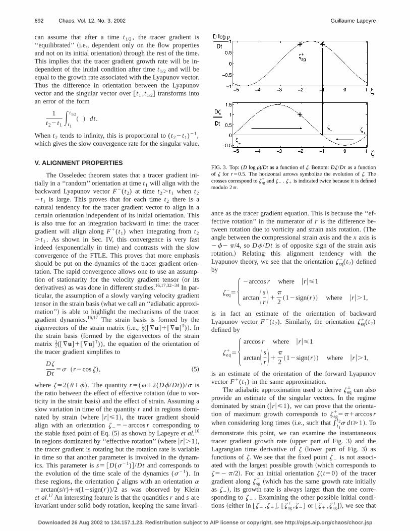
The adiabatic approximation used to derivezeq6 can also
provide an estimate of the singular vectors. In the regidominated by strain (ur u<1), we can prove that the orientation of maximum growth corresponds tozsg
15p1arccosrwhen considering long times~i.e., such that* t1
t2s dt@1!. To
demonstrate this point, we can examine the instantanetracer gradient growth rate~upper part of Fig. 3! and theLagrangian time derivative ofz ~lower part of Fig. 3! asfunctions ofz. We see that the fixed pointz2 is not associ-ated with the largest possible growth~which corresponds toz52 p/2!. For an initial orientationz(t50) of the tracergradient alongzsg
1 ~which has the same growth rate initiallas z2!, its growth rate is always larger than the one corsponding toz2 . Examining the other possible initial condtions ~either in@z2 ,z1#, @zsg
1 ,z2# or @z1 ,zsg1#!, we see that
FIG. 3. Top: (D log r)/Dt as a function ofz. Bottom:Dz/Dt as a functionof z for r 50.5. The horizontal arrows symbolize the evolution ofz. Thecrosses correspond tozsg
1 andz2 . z1 is indicated twice because it is definemodulo 2p.
license or copyright, see http://ojps.aip.org/chaos/chocr.jsp
the time interval can be split into two parts: one for whithe growth rate will be smaller that for the tracer gradieinitially along zsg
1 ; and another one for which it will have thsame behavior as the latter orientation. This argument prothat the orientationzsg
1 should be an estimate of thLyapunov vectorG1 if the adiabatic approximation is validSimilarly, we expectzsg
25p2arccosr to be a good approxi-mation of the backward singular vector in regions wheur u,1. To extend this results to regions dominated by‘‘effective rotation,’’ we can use the orthogonality ofF1 andG1 ~or F2 andG2! so thatzsg
6 should be equal top1zeq6 ,
i.e.,
zsg65H p6arccosr where ur u<1
arctanS s
r D1p
2~32sign~r !! where ur u.1.
This last equality uses the notion of biorthogonality of Frell and Ionnaou.24
To examine these estimates in the numerical simulatwe computed the cosine of twice the relative angle offorward singular vectorg1 with different orientations as afunction of the adimensional timetadim ~Fig. 4!. These ori-entations are the compressional strain axisS2 ~correspond-ing to z52p/2! and the adiabatic solutionszeq
2 andzsg1 , all
of these computed at timet1 . Initially, we observe the sin-gular vectorg1 to be in the direction ofS2. This is an exactresult since (D/Dt) (MTM )(t1 ,t1)52S, and in an expan-sion at a first order in time,MTM5Id12tS1O(t2). Thealignment with the strain eigenvector decreases rapidlytime and after 10 adimensional time units, the average cois only 0.3. During the same period, the average cosine ofadiabatic approximation of the singular vector increasesreach a maximum of 0.8 at about 2 time units and thencreases around 0.5. This demonstrates that our assumptistationarity for the quantityr ~i.e., the adiabatic approximation! seems strictly valid for a few turn-over times but thestimatedzsg
1 direction gives a good estimate of the true sgular vector even for long times. Actually a direct compution of the mean adimensional time of validity of the adbatic assumption~not shown! shows that this time is largethan one turn-over time for 30% of particles and this is ev
FIG. 4. Average cosine between forward singular vectorg1 and adiabaticapproximationzsg
1 , compressional strain eigenvectorS2 and adiabatic equi-librium solutionz2 as a function of adimensional timetadim.
Downloaded 26 Aug 2002 to 134.157.1.23. Redistribution subject to AIP
t
es
ee
-
n,e
innee
toe-
of
--
n
greater~40%! in regions dominated by strain~whereur u,1!.Concerning the backward integration in time, an identievolution is observed~not shown! but the roles are changedinitially the backward singular vectorg2 is aligned withS1
~corresponding toz51p/2!, then it aligned with zsg2
whereas the correlation withzeq1 remains small.
SinceF1(t1) and G1(t1) are orthogonal and sincezeq1
and zsg1 are also orthogonal, the alignment between the f
ward vectorF1 andzeq1(t1) is exactly equivalent to the align
ment betweenzsg1 and the forward vectorG1. Thus, Fig. 4
shows thatzeq1(t1) well approximates the forward Lyapuno
vector F1(t1). Similarly, zeq2(t2) well approximates the
backward Lyapunov vectorF2(t2) ~not shown!, which isconsistent with our previous results.16,17
VI. DIFFERENCES BETWEEN LYAPUNOV VECTORS
A. Singular vectors versus bred modes
In the preceding discussion, two classes of Lyapunvectors were introduced: the ‘‘bred modes’’ associated walignment of the tracer gradient after equilibration@f 2(t2)and f 1(t1) for backward and forward integrations in time#and the singular vectors associated with maximal tracerdient growth over a finite time interval@g2(t2) andg1(t1)#.We can use the adiabatic solutions to gain some insightsthe differences between these vectors.
As was shown by the dynamical argument in Sec. V,orientationszsg
6 are not at all related to an equilibrium: theare associated with a kinematic effect in the sensegrowth rate and orientation properties are out of phasethat the equilibrium orientationszeq
6 do not correspond to thelargest possible growth rate. This is observed in the numcal simulation~Fig. 4! since the correlation ofzeq
2 with g1 isvery weak whereas it is stronger forzsg
6 . Moreover the cor-relation of g1 with f 2 presents the same tendency ascorrelation withzeq
2 ~not shown!. This behavior is related tothe non-normality of¹u ~expressed in the strain basis!, i.e.,the fact that ¹u has nonorthogonal eigenvectors.24 Two limiting cases can highlight these differenceIn a pure strain field~for which r 50!, the orientationszsg
1
andzeq2 are equal, which means that the tracer gradient c
verges toward the vector corresponding to the largest grorate ~the compressional strain axis here!. In this case, theequation of the norm and of the orientation of the gradiare in phase and the velocity gradient in the strain basisorthogonal eigenvectors. For an axisymmetric vortex,situation is quite different sincer equals61 ~see Lapeyreet al.16! and the orientationszeq
2 andzsg1 are now orthogonal.
In this case, the tracer gradient at equilibrium is orthoradwhereas the largest growth over a finite time can be obtaiwhen the gradient is oriented in the radial direction. Itinteresting to note that these two orientations corresponno instantaneous growth of the tracer gradient. This behaindicates the importance of the rotation due to the vorticitythe strain basis~what we call the ‘‘effective rotation’’! indriving the non-normality of the operator. The competitiobetween effective rotation and strain is the main mechanthat drives the difference betweenzeq
2 andzsg1 and seems also
to explain the difference betweenF2 andG1 in the numeri-
license or copyright, see http://ojps.aip.org/chaos/chocr.jsp
tee’’e
nof
e
ha(
-noinn
tefo
t
h
onro
-oeorsrs-t
g
wohao
reet
imthnord
amel
drre-
ndto
theble
ta-
as
meems ineo-
in
fla-
gecal
f thehesof
tseir
ted,
694 Chaos, Vol. 12, No. 3, 2002 Guillaume Lapeyre
cal simulation. The orientationsg6 ~and G6! are thereforenot instructiveper seto understand the dynamics associawith Lyapunov theory. They correspond to the ‘‘extrembehavior for the tracer gradient whereas the Lyapunov vtorsF6 correspond to the equilibrated~or ‘‘mean’’! behavior.
B. Backward versus forward vectors
There also exists a distinction between forward abackward Lyapunov vectors. The Osseledec theorem shthat these vectors are associated with different propertiesforward and backward integration in time but these propties are not directly comparable.
Again we can use the adiabatic approximation to empsize the differences. In the case of a pure strain fieldr50), the backward orientationzeq
2 and the forward orientation zeq
1 are orthogonal corresponding to the compressioand extensional strain axes. In this situation, they correspto orientations of growth for the tracer gradient, eitherbackward or forward integration in time. For the more geeral caseur u,1, the equilibrium orientationszeq
6 are differentand also correspond to growth of the tracer gradient ingrated forward or backward in time. On the other hand,an axisymmetric vortex, the two orientationszeq
6 are equal.For the more general case ofur u.1, zeq
6 are also equal buthe forward growth rate (D/Dt) logu¹qu52s sinzeq
2
52s s/Ar 21s2 is strictly opposite to the backward growtrate 2 (D/Dt) logu¹qu5s sinzeq
15s s/Ar 21s2 ~as time isreversed!. This is because a growth in a forward integraticorresponds to a decay in a backward integration in thistation regime.
The difference betweenzeq2 andzeq
1 relates to the reversibility or irreversibility of the tracer gradient dynamics. Swe can interpret the difference between the Lyapunov vtorsF2 andF1 to be a consequence of local reversibilityirreversibility of the flow ~of course, if a trajectory passefrom a region with chaotic behavior to a region with reveible behavior, it is globally chaotic!. To diagnose such a behavior we can compare the instantaneous growth rate oftracer gradient at timet when integrated from the past~i.e.,from time t1 such thatt2t1.0 is large! with the growth rateat time t when integrated from the future~i.e., from timet2
such that t22t is large!. This corresponds to comparin(D/Dt) logu¹qu for an orientation along F2(t) and2 (D/Dt) logu¹qu for an orientation alongF1(t) @Eckhardtand Yao35 introduced the growth rate alongF2(t) to measurea local Lyapunov exponent for a different purpose#. Figure 5presents the joint probability density function of these tquantities computed after a time integration such t* t1
t s rmsdt5* tt2s rmsdt520. As expected, we observe tw
different regimes: a regime along the anti-bisector corsponding to opposite growth rates. This means that in thregions, the dynamics is instantaneously nonchaotic, andbehavior of the gradients is reversible. The second regcorresponds to the large branch along the bisection inpositive quadrant corresponding to growths forward abackward in time. These regions are associated with strirreversibility of the system, since if we integrate forwa
Downloaded 26 Aug 2002 to 134.157.1.23. Redistribution subject to AIP
d
c-
dwsorr-
-
alnd
-
-r
-
c-
-
he
t
-seheee
dng
and backward the tracer gradient equations along the strajectory, we will obtain a different solution than the initiacondition.
We tried to relate the two regimes to the quantityr andfound that the regions of irreversibility are well correlatewith ur u,1 whereas the regions more predictable are colated withur u.1 ~not shown!. The numerical simulation thusconfirms the prediction of the adiabatic approximation ashows that forward and backward Lyapunov vectors tendhave same sign or opposite sign growth rates but withsame amplitude. This could explain why stable and unstainvariant manifolds often display the same orientation~asshould be the case in regions dominated by ‘‘effective rotion’’ ! whereas they intersect near hyperbolic points~as theycorrespond to different or even orthogonal orientationsshould be the case in regions dominated by strain!.
VII. SPATIAL DISTRIBUTION OF FTLEs
There have been numerous studies of finite tiLyapunov exponents in two dimensions but most of thconcentrated on the statistics of the Lyapunov exponentrelation to the tracer field.31,36–38Some of them examined thspatial distribution of the Lyapunov exponents in a twdimensional chaotic flow.8,25To our knowledge, we give herethe first description of the spatial distribution of FTLEfreely decaying turbulence. Only Babianoet al.39 examinedsome particular trajectories for this type of flow.
The time evolution of the spatial distribution oLyapunov exponents is very similar in our turbulent simutions to that found by Pierrehumbert and Yang8 in their cal-culation for the troposphere: for small time integration, larFTLEs ~Fig. 5! concentrate in patches with shapes identito the distribution of the strain rate~not shown!. This isbecause the strain rate controls the short-term behavior osingular value as explained in Sec. V. Then, these patcbecome thinner and thinner and transform into filamentslarge FTLEs~see Fig. 6!. As time proceeds, these filamenbecome narrower and fill the background flow but th
FIG. 5. Joint PDF of the forward and backward growth rates compurespectively, with an orientation alongF2 andF1.
license or copyright, see http://ojps.aip.org/chaos/chocr.jsp
FIG. 6. Finite time Lyapunov expo-nent fortadim56, plotted at initial po-sitions.
eonioaoie
ex
anurur
eea
ente
ig
e
ofio
ege
tohe
tomblendndri-topdsthetop
o ain-nero-it.
ntslly
or-td
s of
irther-the
LE-
Lyapunov exponents decrease and tend to the spatial mvalue as particles are experiencing different straining regi~not shown!. This process shows that spatial homogenizatof the Lyapunov exponent proceeds rapidly as particles htime to wander through the flow. Then, the Lyapunov expnent of the particles will slowly decay as the turbulencealso decaying. Finally, the FTLE field will tend to the valul`50. Figure 6 displays the FTLE after a timetadim56 ~themost interesting stage in our opinion! corresponding to thepresence of filaments with large values of the Lyapunovponents~compared with the spatial mean exponent^l&'1!.For reference, the pdf of FTLEs corresponds to the bolddashed curve in Fig. 2. The filaments present in the figcould be the signature of the invariant manifolds in the tbulent flow field.
Concerning the spatial distribution of the FTLEs, thrdifferent categories of structures can be described. Therelarge scale filaments that correspond to the largest exponThese filaments start from the neighborhood of one vorand end close to the vicinity of another vortex~see, for in-stance, the long and horizontal filament in the center of F6!. They are associated with theinteraction of vorticeswhichleads to a large straining. This can be demonstrated byamining the Lyapunov exponent at thefinal positions of par-ticles att2 ~Fig. 7! ~actually this figure represents the normthe gradient of a real tracer during the stage where diffusdoes not play any role!. The very long filament starting fromthe top of Fig. 7 and ending at the bottom near the asymmric dipole corresponds to the horizontal filament with larFTLE on Fig. 6. As trajectories indicate~not shown!, theformation of the dipole of the bottom center of Fig. 7 leadsthe ejection of material and to this very long filament. T
Downloaded 26 Aug 2002 to 134.157.1.23. Redistribution subject to AIP
ans
nve-s
-
de-
rets.x
.
x-
n
t-
same process occurs with the two vortices at the botright- and left-hand corners of Fig. 6, which are responsifor the filament at the top right-hand corner of Fig. 6 awhich lead to the dipole at the bottom right- and left-hacorners of Fig. 7~remember that the domain is doubly peodic!. A last example corresponds to the vortex at thecenter of Fig. 6: a filament starts from this vortex and enup near the two smaller vortices close to the center offigure. In Fig. 7, we see that these three vortices at thecenter of the figure are very close at this time, leading tvery strong straining. These FTLEs that start from the vicity of one vortex and terminate at the vicinity of another oare due to the future interactions of these vortices that pvide the straining and nonlocal transport associated with
Another kind of structure corresponds to the filamethat wind up around the vortices in spirals. This is generathe case for vortices that are close to axisymmetric shape~forinstance the vortex at the center of Fig. 6!. These filamentsare associated with ejection of material from inside the vtex to its surroundings, thus they materialize the transporinthe vicinity of the vortex. They are densely packed arounvortices and the vortex core is characterized by low valueLyapunov exponents, consistent with Babianoet al.39 Par-ticles seeded uniformly in a box around the vortex~Fig. 8!tend to stay in the vicinity of the vortex even if theLyapunov exponent is high. Some particles even entervicinity by the interplay of the large scale filament. The votex core is well defined as particles do not generally leavecore and have low FTLEs~see the particles in gray in Fig. 8!.We therefore speculate that the layered structure of FTaround the circular vortices is just the ‘‘circulating cell’’ described by Elhmadiet al.2 or the ‘‘stochastic layer’’ dis-
license or copyright, see http://ojps.aip.org/chaos/chocr.jsp
696 Chaos, Vol. 12, No. 3, 2002 Guillaume Lapeyre
FIG. 7. Finite time Lyapunov expo-nent fortadim56, plotted at final posi-tions.
-:ngisla-
a
deso
beicath
e. Irretu.f
ien
thtotu
onus-
eor-certionpo-ori-ovr’’oso-lib-f-laras
en-tionxi-ofer--
ehends
dther-la-e of
cussed by Joseph and Legras.14 This region controls the exchange between the far field and the interior of the vortexparticle that exits a vortex core is trapped for a very lotime in that region before it is expelled to the far field. Itinteresting to note that elliptical vortices have a few fiments that wind up around them, and their edges~i.e., theircirculating cell! seem thinner. These elliptical vortices havegeometrical structure very similar to the Kida vortex15,40
with two long filaments surrounding the vortex and extening to the far field. This circulating cell around the vorticcould act as a dynamical barrier: a circular shape is assated with a thick stochastic layer that prevents mixingtween the vortex core and the far field whereas an elliptshape is associated with a thinner layer and the interior ofvortex can be mixed more easily with the far field.
A last category of structures corresponds to low valuof Lyapunov exponents in the background turbulent fieldis associated with low values of the strain rate and cosponds to vortices of smaller and smaller scale and amplibut with properties analogous to the large scale vortices
Finally, the distribution of FTLEs shows the intricacy ochaotic mixing in two-dimensional turbulence: the propertof mixing depend not only on the shape of the vortices atheir stochastic layer but also on the nonlocal interactionallows mixing to spread from the vicinity of one vortexanother one. The FTLE with largest values are the signaof the future interactions between coherent structures.
VIII. CONCLUSION
We have discussed the link between recent resultstracer gradient dynamics and Lyapunov theory using americal simulation of two-dimensional turbulence to illu
Downloaded 26 Aug 2002 to 134.157.1.23. Redistribution subject to AIP
a
-
ci--le
st-
de
sdat
re
n-
trate our points. Lyapunov theory predicts not only the timevolution of the norm of the tracer gradient but more imptantly the existence of orientations toward which the tragradient converges. The rapid convergence of the orientacontrasts with the slow convergence of the Lyapunov exnent and justifies the importance of the dynamics of theentation. Two types of structures emerge from Lyapuntheory: singular vectorsg6 associated with maximum tracegradient growth over a finite time and ‘‘linear bred modevectorsF6 toward which tracer gradients align. These twtypes are intrinsically different because the first one is asciated with extreme behavior and the other one with equirium ~or ‘‘mean’’! behavior of the tracer gradient. This diference is due to the importance of strain for the singuvectors and effective rotation for stable Lyapunov vectorsthe numerical simulations confirms it. Moreover, these oritations can be estimated from local velocity and acceleragradient tensors by the so-called ‘‘adiabatic appromation.’’ 16,17Another point is that the relative orientationsforward and backward Lyapunov vectors allow one to detmine the local ‘‘irreversibility’’ of the tracer gradient dynamics.
We also examined the spatial distribution of finite timLyapunov exponents in the two-dimensional flow field. TFTLEs present an intricate structure which strongly depeon the shape of the vortices for local transport~i.e., in thevicinity of the vortex!: nearly circular vortices have a broacirculating cell which seems to prevent mixing betweenfar field and the interior of the vortex whereas elliptical votices have a narrow circulating cell. Some large scale fiments of large values of FTLE are also present becaus
license or copyright, see http://ojps.aip.org/chaos/chocr.jsp
FIG. 8. Initial ~left! and final~right! positions of particles seeded near the circular vortex of the center of Fig. 6.
c
rywo
e
ta
noexag
ryy
p-iem
ior
man
ne
f t.de
con-ell
esd
ein
ty. Iienoned.
ed
ofle-
n
ev.
ds,’’
ort
ic
-
the interaction between vortices and govern the nonlotransport properties.
Finally, this paper tried to clarify what Lyapunov theocan teach us for the properties of chaotic advection by tdimensional flows. The Lyapunov approach was usedmany studies but with different points of view. ThOkubo32–Weiss33 ~OW! criterion and the Hua and Klein~HK!34 criterion were introduced to understand the instanneous dynamics of the tracer gradient related tolocal growthor rotation of the gradient. However, these criteria aredirectly related to Lyapunov exponents as the Lyapunovponents correspond to a tracer gradient growth rate averalong a Lagrangian trajectory, which isnonlocal by nature.This explains why finite time Lyapunov exponents give vedifferent results from OW and HK criteria as illustrated bBoffetta et al.41 The Okubo–Weiss and Hua and Klein aproaches were indeed relevant for the dynamics of the ortation of the Lyapunov vectors as the dynamics is decoposed by these criteria in terms of the competition of rotatand strain. This competition drives the dynamics of the oentation of the tracer gradient~see Lapeyreet al.,16 Kleinet al.,17 and Sec. V of the present paper!. To recover theLyapunov exponent, one then needs to integrate the infortion of the dynamics of the orientation along Lagrangitrajectories through the tracer gradient growth rate. Thisbasically the approach followed by Lapeyreet al.15 This kindof approach for studying transport barriers or invariant mafolds is preferable than directly diagnosing finite timLyapunov exponents because of the slow convergence oFTLE as shown by Boffettaet al.41 for a nontrivial test caseOther alternative approaches exist, such as the methoHaller13,42 to diagnose invariant manifolds, the finite siz
Downloaded 26 Aug 2002 to 134.157.1.23. Redistribution subject to AIP
al
-in
-
t-ed
n--
ni-
a-
is
i-
he
of
Lyapunov exponent technique,9,41 or effective diffusivity.43,44
These methods give good results because of their fastvergence in time but their basic properties are not yet wunderstood.
ACKNOWLEDGMENTS
This work was initiated in Laboratoire of Physique dOceans~France!. The numerical simulations were performeat IDRIS ~CNRS!, Orsay, France. During the writing of thpaper, I was supported by the Visiting Scientist ProgramAtmospheric and Oceanic Sciences at Princeton Universiam grateful for numerous thoughtful suggestions from LHua and Patrice Klein. Discussions with Bernard Legrasthe concept of dynamical barrier are also acknowledgBrian Arbic improved the manuscript with his comments.
1R. T. Pierrehumbert, ‘‘Chaotic mixing of tracer and vorticity by modulattravelling Rossby waves,’’ Geophys. Astrophys. Fluid Dyn.58, 285~1991!.
2D. Elhmaıdi, A. Provenzale, and A. Babiano, ‘‘Elementary topologytwo-dimensional turbulence from a Lagrangian viewpoint and singparticle dispersion,’’ J. Fluid Mech.257, 533 ~1993!.
3Z. Neufeld and T. Te´l, ‘‘Advection in chaotically time-dependent opeflows,’’ Phys. Rev. E57, 2832~1998!.
5T. Tel, G. Karolyi, A. Pentek, I. Scheuring, Z. Toroczkai, C. Grebogi, anJ. Kadtke, ‘‘Chaotic advection, diffusion, and reaction in open flowChaos10, 89 ~2000!.
6H. Aref, ‘‘Stirring by chaotic advection,’’ J. Fluid Mech.143, 1 ~1984!.7J. M. Ottino,The Kinematics of Mixing: Stretching, Chaos and Transp~Cambridge University Press, Cambridge, 1989!.
8R. T. Pierrehumbert and H. Yang, ‘‘Global chaotic mixing on isentropsurfaces,’’ J. Atmos. Sci.50, 2462~1993!.
9V. Artale, G. Boffetta, A. Celani, M. Cencini, and A. Vulpiani, ‘‘Disper
license or copyright, see http://ojps.aip.org/chaos/chocr.jsp
nt
-
anpl
y
st
e
to
rs
bls,
o
tic
i-s
a
gser
o
o
a-
d
e
ovical
ov
ar,s,’’
f. Ab-
ro-
f
s,’’
ticys.
the
c-ids
.
rs
ity
bil-
of
698 Chaos, Vol. 12, No. 3, 2002 Guillaume Lapeyre
sion of passive tracers in closed basins: Beyond the diffusion coefficiePhys. Fluids9, 3162~1997!.
10J. Guckenheimer and P. Holmes,Nonlinear Oscillations, Dynamical Systems, and Bifurcations of Vector Fields~Springer, New York, 1983!.
11S. Wiggins,Chaotic Transport in Dynamical System~Springer, New York,1992!.
12N. Malhotra and S. Wiggins, ‘‘Geometric structures, lobe dynamicsLagrangian transport in flows with aperiodic time dependence, with apcations to Rossby wave flow,’’ J. Nonlinear Sci.8, 401 ~1998!.
14B. Joseph and B. Legras, ‘‘Relation between kinematic boundaries,ring and barriers for the Antartic polar vortex,’’ J. Atmos. Sci.59, 1198~2002!.
15G. Lapeyre, B. L. Hua, and B. Legras, ‘‘Comments on ‘Finding finite-timinvariant manifolds in two-dimensional velocity fields,’ ’’ Chaos11, 427~2001!.
16G. Lapeyre, P. Klein, and B. L. Hua, ‘‘Does the tracer gradient vecalign with the strain eigenvectors in 2-D turbulence?’’ Phys. Fluids11,3729 ~1999!.
17P. Klein, B. L. Hua, and G. Lapeyre, ‘‘Alignment of tracer gradient vectoin 2D turbulence,’’ Physica D146, 246 ~2000!.
18A. Adrover and M. Giona, ‘‘Measure-theoretical properties of the unstafoliation of two-dimensional differentiable area-preserving systemPhys. Rev. E60, 347 ~1999!.
19G. Haller, ‘‘Lagrangian structures and the rate of strain in a partitiontwo-dimensional turbulence,’’ Phys. Fluids13, 3365~2001!.
21F. Varosi, T. M. Antonsen, Jr., and E. Ott, ‘‘The spectrum of fractal dmensions of passively convected scalar gradients in chaotic fluid flowPhys. Fluids A3, 1017~1991!.
22J.-P. Eckmann and D. Ruelle, ‘‘Ergodic theory of chaos and strangetractors,’’ Rev. Mod. Phys.57, 617 ~1985!.
23B. Legras and R. Vautard, ‘‘A guide to Liapunov vectors,’’in Proceedinof the 1995 ECMWF Seminar on Predictability, edited by T. PalmReading, U.K., 1996, pp. 143–156.
24B. F. Farrell and P. J. Ioannou, ‘‘Generalized stability theory. I. Autonmous operators,’’ J. Atmos. Sci.53, 2025~1996!.
25G. Voth, G. Haller, and J. P. Gollub, ‘‘Experimental measurementsstretching fields in fluid mixing,’’ Phys. Rev. Lett.88, 254501~2002!.
26B. L. Hua, ‘‘The conservation of potential vorticity along Lagrangian trjectories in simulations of eddy-driven flows,’’ J. Phys. Oceanogr.24, 498~1994!.
Downloaded 26 Aug 2002 to 134.157.1.23. Redistribution subject to AIP
,’’
di-
ir-
r
e’’
f
,’’
t-
,
-
f
27X. Z. Tang and A. H. Boozer, ‘‘Finite time Lyapunov exponent anadvection-diffusion equation,’’ Physica D95, 283 ~1996!.
28J. L. Thiffeault and A. H. Boozer, ‘‘Geometrical constraints on finite-timLyapunov exponents in two and three dimensions,’’ Chaos11, 16 ~2001!.
29I. Goldhirsch, P.-L. Sulem, and S. A. Orszag, ‘‘Stability and Lyapunstability of dynamical systems: A differential approach and a numermethod,’’ Physica D27, 311 ~1987!.
30S. V. Ershov and A. B. Potapov, ‘‘On the concept of stationary Lyapunbasis,’’ Physica D118, 167 ~1998!.
31G.-C. Yuan, K. Nam, T. M. Antonsen, Jr., E. Ott, and P. N. Guzd‘‘Power spectrum of passive scalars in two dimensional chaotic flowChaos10, 39 ~2000!.
32A. Okubo, ‘‘Horizontal dispersion of floatable particles in the vicinity ovelocity singularity such as convergences,’’ Deep-Sea Res. Oceanogrstr. 17, 445 ~1970!.
33J. Weiss, ‘‘The dynamics of enstrophy transfer in two-dimensional hyddynamics,’’ Physica D48, 273 ~1991!.
34B. L. Hua and P. Klein, ‘‘An exact criterion for the stirring properties onearly two-dimensional turbulence,’’ Physica D113, 98 ~1998!.
35B. Eckhardt and D. Yao, ‘‘Local Lyapunov exponents in chaotic systemPhysica D65, 100 ~1993!.
36T. M. Antonsen, Z. Fan, E. Ott, and E. Garcia-Lopez, ‘‘The role of chaoorbits in the determination of power spectra of passive scalars,’’ PhFluids 8, 3094~1996!.
37K. Ngan and T. G. Shepherd, ‘‘A closer look at chaotic advection instratosphere. I. Statistical diagnostics,’’ J. Atmos. Sci.56, 4153~1999!.
38R. T. Pierrehumbert, ‘‘Lattice models of advection-diffusion,’’ Chaos10,61 ~2000!.
39A. Babiano, G. Boffetta, A. Provenzale, and A. Vulpiani, ‘‘Chaotic advetion in point vortex models and two-dimensional turbulence,’’ Phys. Flu6, 2465~1994!.
40S. Kida, ‘‘Motion of an elliptic vortex in a uniform shear flow,’’ J. PhysSoc. Jpn.50, 3517~1981!.
41G. Boffetta, G. Lacorata, G. Redaelli, and A. Vulpiani, ‘‘Detecting barrieto transport: A review of different techniques,’’ Physica D159, 58 ~2001!.
43N. Nakamura, ‘‘Two-dimensional mixing, edge formation and permeaity diagnosed in an area coordinate,’’ J. Atmos. Sci.53, 1524~1996!.
44P. H. Haynes and E. Shuckburgh, ‘‘Effective diffusivity as a diagnosticatmospheric transport. 1. stratosphere,’’ J. Geophys. Res.,@Atmos.# 105,22777~2000!.
license or copyright, see http://ojps.aip.org/chaos/chocr.jsp


![Cellular automata and Lyapunov exponents arXiv:math ... · PDF filearXiv:math/0312136v1 [math.DS] 6 Dec 2003 Cellular automata and Lyapunov exponents P. TISSEUR Institut de Math´ematiques](https://static.documents.pub/doc/80x56/5a9df39a7f8b9adb388c437c/cellular-automata-and-lyapunov-exponents-arxivmath-math0312136v1-mathds.jpg)


