Characterization of LMR Analog FM Audio Quality … of LMR Analog FM Audio Quality Using PL Tone...

Characterization of LMR Analog FM Audio QualityUsing PL Tone Analysis

Akshay Kumar Steven [email protected] [email protected]

Virginia Tech, Wireless@VTMay 2, 2012

Table of Contents1 Introduction 3

2 System Model 4

3 Characterization of PL Tone SNR 63.1 Parametric Estimation and Subtraction (PE/S) Method . . . . . . . . . . . . . . . 63.2 Method of Kurtosis . . . . . . . . . . . . . . . . . . . . . . . . . . . . . . . . . . 73.3 Theoretical Method . . . . . . . . . . . . . . . . . . . . . . . . . . . . . . . . . . 8

4 Results 104.1 Simulated Signal . . . . . . . . . . . . . . . . . . . . . . . . . . . . . . . . . . . 10

4.1.1 Ideal Conditions . . . . . . . . . . . . . . . . . . . . . . . . . . . . . . . 104.1.2 Including effects of FM modulation/demodulation process (stationary chan-

nel) . . . . . . . . . . . . . . . . . . . . . . . . . . . . . . . . . . . . . . 124.1.3 Including effects of Rayleigh fading channel . . . . . . . . . . . . . . . . 19

4.2 Actual LMR Signals . . . . . . . . . . . . . . . . . . . . . . . . . . . . . . . . . 194.2.1 Control Experiment . . . . . . . . . . . . . . . . . . . . . . . . . . . . . . 194.2.2 Actual Signals . . . . . . . . . . . . . . . . . . . . . . . . . . . . . . . . 20

5 Conclusion 31

ii

1 Introduction

This report documents some practical techniques for characterizing the land mobile radio (LMR)analog FM audio quality using Private Line (PL) tone analysis. A particular application where thisis desirable is the antenna system project [1], which requires on-the-air testing in a TIA-603 analogsystem. In this project, it is desirable to have a “bottom line” assessment of the audio quality inorder to accurately determine in-situ RF signal to noise ratio (SNR). The audio signal is not knowna priori, making it difficult to gauge the audio quality. To overcome this, one can use the existing“PL tone” which is injected in the sub-audio band along with the audio signal before transmission.At the receiver, this PL tone can be analyzed to get an audio SNR metric independent of the voicesignal. The audio SNR can also be converted into an RF SNR, which will be the topic of a separatememo.

This report discusses two practical techniques for estimating the SNR of the PL tone. The firstmethod is the parametric estimation and subtraction (PE/S) method. In this method, the parametersof the PL tone – amplitude, frequency and phase – are estimated, and then a noise free copy of thePL tone is locally synthesized. It is then subtracted coherently from the filtered PL tone leavingbehind the sub-audio noise. SNR is then the ratio of the estimated PL tone power to the subaudionoise power. The second method involves measuring the kurtosis of the filtered PL tone and usingthen that to calculate the audio SNR. Both these methods are first tested through simulations, andapplied to the actual LMR signals.

Figure 1 shows the dynamic spectrum of an actual off-the-air FM signal. The PL tone is clearlyvisible in the spectrum throughout the duration of the signal except for small durations of approx-imately 0.1 s when one speaker switches to the other. PL tone frequencies range from 67 Hz to257 Hz.

The rest of the document is organized as follows. Section 2 describes the simulation model of theFM communication system used in our work. Section 3 details the techniques used to characterizethe audio quality. Section 4 compares the techniques described in Section 3 by first applyingthem to simulated data and then against captured LMR signals. Finally Section 5 summarizes theperformance of the experimental techniques.

3

Figure 1: Dynamic spectrum of an audio signal. In this case, the PL tone frequency is 162.2 Hz.

2 System Model

Figure 2 shows the model of the FM communication system used in our work.

There are two inputs to the model – the message signal and the carrier. The message signal consistsof the audio signal and the PL tone. The FM modulator varies the carrier frequency in proportionto the amplitude of the message signal. If m(t) is the message signal and c(t) = Ac cos(2πfct) isthe carrier, then the modulated signal is given by

sFM(t) = Ac cos(2πfct+ kfm

∫ t

−∞m(t)dt), where (1)

kfm =2π∆f

mp

(2)

is the modulation index. ∆f is the maximum frequency deviation, and mp is the maximum ampli-tude of m(t). The complex baseband representation of the FM modulator in equation (1) is

sFM,bb(t) = Ace(jkfm

∫ t−∞m(t)dt). (3)

The transmitted signal is distorted by the communication channel which is of Rayleigh flat fadingtype, and then mixed with additive white Gaussian noise (AWGN). A reformulated Jakes fadingmodel, proposed by Dent (1993) [2], is used to simulate the Rayleigh fading channel. The model

4

Akshay

Line

Akshay

Text Box

PL tone

Audio Input (Voice+PL tone)

Audio Output

FM Modulator

Carrier Generator

Propagation Channel (AWGN/Rayleigh Fading)

IF Filter

FM Detector

Audio Filter

Figure 2: System Model

assumes that N equal-strength rays arrive at the receiver with uniformly distributed arrival anglesαn, such that the ray n experiences a Doppler shift ωn = ωmcos(αn), where ωm = 2πfcv/c is themaximum Doppler shift, v is the relative speed of receiver with respect to the transmitter, and c isthe speed of light. The resulting channel coefficient is:

T (t) =√

2/No

No∑n=1

ejβncos(ωn + θn) (4)

where No = N/4 is the number of equal strength complex oscillators needed to produce themultiple waveforms and the normalization factor

√2/No gives E[T (t)T ∗(t)] = 1. By using β =

πn/No, the real and imaginary parts of T (t) have equal power and are uncorrelated. Setting αn =2π(n − 5)/N provides quadrantal symmetry for all of the arriving waveforms. Randomizing θnprovides different waveform realizations.

The received FM signal is then filtered by a flat-topped band-pass “IF” filter, centered at the carrierfrequency and with bandwidth equal to that of the FM signal (approximated by Carson’s formula).The filtered signal is then fed into the FM demodulator, implemented as sequence of DSP opera-tions as follows:

Let r(n) be the complex valued discrete signal at the output of the IF filter, where n representsdiscrete time instants. Then if rr(n) and ri(n) are respectively the real and imaginary parts ofr(n), we have

rs(n) = ri(n) rr(n− 1)− rr(n) ri(n− 1), (5)rc(n) = rr(n) rr(n− 1)− ri(n) ri(n− 1), (6)g1(n) = rs(n)/rc(n), (7)g2(n) = arc tan(g1(n)), (8)y(n) = g2(n)/(T kfm) (9)

5

where T = 1/fs, fs being the sampling frequency. The output of the demodulator y(n) is thenpassed through an audio filter which is a Chebyshev finite impulse response (FIR) low-pass filterof order 803 and with 3-dB bandwidth set to 3.5 kHz.

3 Characterization of PL Tone SNR

The output signal of the audio filter in our system model consists of the audio signal including thePL tone. Then we filtered out the audio signal using a Chebyshev FIR low-pass filter of order 1607and with 3-dB bandwidth set to 250 Hz. Next, the SNR of the PL tone is determined using thefollowing experimental techniques.

3.1 Parametric Estimation and Subtraction (PE/S) Method

This method is particularly suitable when the signal to be estimated can be described in a simplemathematical form with only a small number of slowly-varying parameters. In this case, we mayassume a sinusoid where the parameters are amplitude, frequency and phase. These parametersare optimally estimated and a noise-free copy is locally synthesized. The estimated signal is thensubtracted coherently from the original signal, nominally leaving the noise.

The input signal is modeled as

x(t) = s(t) + n(t), (10)s(t) = ae(j(ωt+θ)) (11)

where s(t) is the signal to be estimated having a, ω, and θ as the magnitude, frequency and phaserespectively. n(t) is the noise, assumed to be Gaussian. Then the optimal estimates of the parame-ters a, ω and θ are given by

ω = arg maxω

∣∣⟨x(t)e(−jωt)⟩∣∣ , (12)

a =∣∣⟨x(t)e(−jωt)

⟩∣∣ , (13)

θ = ∠⟨x(t)e(−jωt)

⟩, (14)

where the angle brackets < . > denote time averaging.

In radio communications, the received radio signal is generally not stationary over long durationsof time. This is due to the fading environment; specifically, by time-varying multipath. To ac-commodate this, we apply the PE/S method repeatedly within short segments of the signal duringwhich it can be assumed to be approximately stationary. An example of this approach is discussedin Lee (2008) [3] in the context of mitigation of RF interference.

6

3.2 Method of Kurtosis

In this method, the kurtosis is used to calculate the SNR for the signal, as discussed in Matzner(1994) [4]. In this case, both s(t) and n(t) in equation (10) are assumed to be real, stationary, zeromean and mutually independent; the latter at least with respect to the fourth order statistics.

Since the sum of independent random processes corresponds to the product of the respective char-acteristic functions, we have:

φx(ω) = φs(ω)φn(ω), (15)

where φx(ω), φs(ω), φn(ω) are the characteristic functions of x(t), s(t), and n(t) respectively. Thecharacteristic function φx(ω) of a random process x(t) having a probability density function (pdf)fX(x), is expanded in a series of its moments as:

φx(ω) =

∫ ∞−∞

fX(x)e−jωxdx =∞∑k=0

(−j)kmx,kωk

k!, (16)

where mx,k is the k-th order moment of x(t). For a discrete signal x[n], mx,k can be computedas:

mx,k =1

N

N∑n=1

|x[n]|k , (17)

where N is the sample size.

It requires simple algebra to show using equations (15) and (16) that the k-th order moment of thesum x(t) in equation (10) is given by

mx,k =k∑l=0

(k

l

)ms,lmn,k−l . (18)

If we evaluate equation (18) for k = 2 and k = 4 and use the assumption that both signal and noiseare zero mean, we find

mx,2 = ms,2 +mn,2 and (19)mx,4 = ms,4 +mn,4 + 6ms,2mn,2 . (20)

The kurtosis Kx of x(t) is defined as

Kx = mx,4/m2x,2 . (21)

Using equation (21) we obtain from equations (19) and (20)

(Kx − 3) = (Ks − 3)κ2 + (Kn − 3)(1− κ)2 , (22)

where κ = ms,2/(ms,2 + mn,2) is related to the SNR we seek. To simplify equation (22), letP = (Kx − 3), Q = (Ks − 3), and R = (Kn − 3). Then solving for κ gives us

κ = (R±√P (Q+R)−QR)/(Q+R) (23)

7

Since the noise is assumed to be Gaussian and the signal, s(t), is a sinusoid (PL tone), Kn = 3 andKs = 1.5. So R = 0 and Q = −1.5. Substituting these values in equation (23), we get

κ =√

(3−Kx)/1.5 . (24)

Now the SNR of the received signal x(t) is given by

SNR = κ/(1− κ) . (25)

Summarizing, the procedure for obtaining SNR from the data, x(t), is as follows:

1. Compute the moments mx,4 and mx,2 using equation (17) for k = 2 and k = 4 respectively.2. Determine the kurtosis from equation (21).3. κ =

√(3−Kx)/1.5 from equation (24).

4. SNR = κ/(1− κ) from equation (25).

As described in Section 3.1, when the received signal is subjected to a time-varying fading (non-stationary) channel, we partition the received signal into small segments over which it is effectivelystationary, and then this method is applied independently to each of these segments. The lengthof the interval over which the partition SNRs are calculated must be chosen carefully as describedpreviously (for PE/S method).

3.3 Theoretical Method

In this section, we present a theoretical method for the estimation of the audio SNR directly fromthe RF SNR. We make the following assumptions in our model (Figure 2):

1. The modulation index for the FM system is greater than unity. This holds true for the TIA-603 modulations.

2. The IF filter has a Gaussian-shaped frequency response, G(f), given by:

G(f) = e−4π(f−fc)2/9B2

, (26)

whereB is the 3-dB IF bandwidth in Hz. We lose little generality by making this assumptionsince the audio filter bandwidth is usually narrow relative to the IF bandwidth.

As the IF SNR falls and goes below the threshold, the signal modulation is suppressed. So thesignal output from the discriminator, mo(t), is given by [5, 6]:

mo(t) = m(t)(1− e−ρ), (27)

where m(t) is the input message signal. Hence the output baseband signal power, S0, is related tothe input modulation signal power, S, as:

So = (1− e−ρ)2S (28)

8

where ρ is the predetection SNR (at the output of the IF filter). Let c denote the transfer character-istic (gain) of the differentiator. c = 2πc

′ , where c′ is a constant with units of Hz/V. Let σm denotethe rms frequency deviation of the signal c′m(t)). Hence its power is σ2

m. Then the IF bandwidthused is chosen according to the formula B = 2(W + σm

√10), where W is the cutoff frequency of

the low pass audio filter. This ensures that modulation peaks less than σm + 10 dB are containedwithin the deviation given by Carson’s rule for sinusoidal modulation. Thus we have,

S =σ2m

c′2, (29)

=4π2σ2

m

c2, (30)

=π2(B − 2W )2

10c2. (31)

Rice in [7] divided the one-sided baseband noise spectrum, P (f), into three components:

P (f) = P1(f) + P2(f) + P3(f). (32)

P1(f) has the same spectrum shape as the output noise spectrum when the carrier is absent. P2(f)has the shape of the output noise spectrum when the carrier is very large,

P2(f) = (1− e−ρ)2Pmo(f), (33)

where Pmo(f) is the output noise spectrum when ρ� 1, and is given by [5]:

Pmo(f) =2π2f 2e−4π(f−fc)

2/9B2

c2Bρ. (34)

P3(f) is a correction term that predominates in the threshold region of ρ. Davis in [6] has shownthat in the frequency range from 0 to W , where W < B, the spectral components P1(f) + P3(f)may be accurately approximated by

PD(f) ≈ 8πBe−ρ[c4√

2(ρ+ 2.35)]−1/2

. (35)

The above approximations may be combined to provide an approximation for the overall basebandnoise spectrum:

P (f) ≈ (1− e−ρ)2Pmo(f) + PD(f) (36)

≈ [2πf(1− e−ρ)]2 e−4π(f−fc)2/9B2

c2Bρ+

8πBe−ρ

c2√

2(ρ+ 2.35)(37)

The total noise power, N , out of a rectangular baseband audio filter is given by:

N(ρ) =

∫ W

0

P2(f)df +

∫ W

0

PD(f)df, (38)

=a(1− e−ρ)2

c2ρ+

8πBWe−ρ

c2√

2(ρ+ 2.35), (39)

9

where using the Maclaurin series expansion, a is given by

a =4π2

B

∫ W

0

f 2e−4π(f−fc)2/9B2

df, (40)

=4π2W 3

3B{1− 4π

15

(W

B

)2

+8π2

189

(W

B

)4

+ ...}. (41)

Since we have assumed that the modulation index is greater than unity, W is much smaller than B.Therefore, we will consider only first three terms in the equation (41) and still get a fairly precisevalue of a. Assuming unit impedance, we verify from equations (31) and (39) that the unit of signaland noise power is watts (W). Now the audio SNR is simply the ratio S0/N . Thus the procedurefor obtaining the audio SNR from predetection SNR, ρ, is as follows:

1. Modulation signal power, S =(π2 (B − 2W )2

)/ (10c2). Since c factors out in the expres-

sion for the audio SNR, we can choose any value for c here. We choose c = 1 here.2. Audio signal power, S0 = (1− e−ρ)2S.3. Compute the audio noise power, N using equations (38) and (40). For calculating a, con-

sider only first three terms in equation (40).4. Audio SNR, SNRa = S0/N .

Figure 3 shows a plot of the audio SNR as a function of predetection SNR using the theoreticalmethod.

4 Results

In this section, we first compare the SNR estimation techniques presented in Section 3 using thesimulated data and later using the actual LMR signals.

4.1 Simulated Signal

4.1.1 Ideal Conditions

Since for simulated data the audio SNR can be precisely controlled, this provides us a “baseline” totest the accuracy of the experimental techniques. Consider the case of a sinusoid in white Gaussiannoise (corresponding to a time-invariant channel). The frequency of the sinusoid is 180 Hz and itsamplitude is varied so that SNR varies from −25 dB to +10 dB. We need to choose the integrationtimes for the PE/S and kurtosis methods prior to estimating SNR. For a mobile radio channel,coherence time varies with the Doppler spread. As a rule of thumb, coherence time, Tc is calculated

10

−10 −5 0 5 10 15 20 25 30−40

−30

−20

−10

0

10

20

30

40

Pre−detection SNR [dB]

Aud

io S

NR

[dB

]

Figure 3: Relationship between audio SNR and predetection SNR using the theoretical result (Non-fading channel). B and W are set to 17 kHz and 3.5 kHz respectively.

11

as [8]:

Tc =0.846π

ωm, where (42)

ωm is the maximum Doppler shift as described in Section 2. Let us define a “best case” fadingscenario over our frequency and velocity range of interest corresponding to a carrier frequencyf = 45 MHz and transmitter velocity v = 1 m/s (vehicle almost stationary). This results in Tc =2800 ms. Let us also define a “worst case” fading scenario corresponding to a carrier frequencyf = 860 MHz and transmitter velocity v = 29 m/s, which results in Tc = 5 ms.

Figures 4–7 compare the experimental SNR, determined using the PE/S and kurtosis methods,against the actual SNR for integration times of 5 ms, 50 ms, 100 ms, and 2800 ms respectively.It is observed that on increasing the integration time, both methods yield accurate results at lowerSNR. For an integration time of 5 ms, PE/S method works well for SNR≥ −15 dB. On increasingthe integration time to 2800 ms, PE/S method gives accurate results for SNR down to −35 dB. Atlow SNR values, the kurtosis result flattens out earlier than the PE/S curve. This is because PE/Sis statistically optimum where as kurtosis is not.

4.1.2 Including effects of FM modulation/demodulation process (stationary channel)

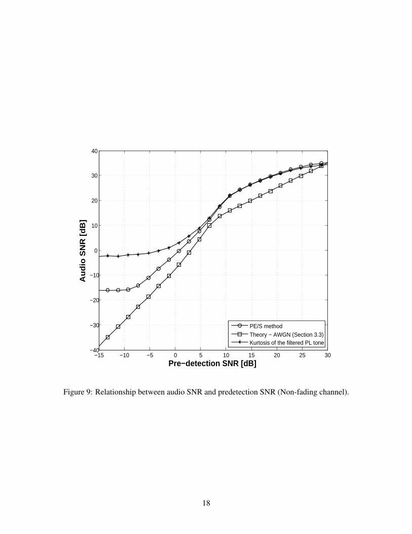
Now we add the process of FM modulation and demodulation to this test case as shown in Figure 2.The channel is assumed to be AWGN with no fading. In equation (3), the message signal m(t)consists of only PL tone with frequency fpl = 180 Hz and amplitude Apl = 1. Also m(t) = 0 fort < 0 s. The amplitude of the carrier, Ac is varied to get a predetection SNR range from −16 dBto 31 dB. We have selected the 138–144 MHz VHF-Hi band for FM transmission. In accordancewith TIA-603B analog FM requirement for maximum deviation and bandwidth [9, 10], we setthe maximum frequency deviation ∆f , and the bandwidth of IF filter, B, to 5 kHz and 17 kHzrespectively. Figure 8 shows the power spectral density (PSD) of the noiseless FM signal.

In Figure 9, we plot the audio SNR as a function of predetection SNR using the PE/S method,the kurtosis method, and the theoretical result. Since the channel is stationary, following from theanalysis done in Section 4.1.1, a reasonable integration times for the PE/S method and the kurtosismethod would be 100 ms. It is observed that the PE/S and kurtosis methods are in close agreementwith each other for predetection SNR > 5 dB. The PE/S and kurtosis curves have nearly sameslope as the theoretical curve and follows it with a 1–5 dB offset, for predetection SNR range from0 dB to 30 dB.

We conclude this section by noting the possibility to use PE/S or kurtosis method to determineaudio SNR and then to use Figure 9 to calibrate from that to the theoretical result.

12

−35 −30 −25 −20 −15 −10 −5 0 5 10−35

−30

−25

−20

−15

−10

−5

0

5

10

Actual SNR [dB]

Estim

ated

SN

R [d

B]

Perfect estimatePE/S methodKurtosis of the noisy sinusoid

Figure 4: Plot of experimental SNR against actual SNR of a noisy sinusoid. Integration time is5 ms.

13

−35 −30 −25 −20 −15 −10 −5 0 5 10−35

−30

−25

−20

−15

−10

−5

0

5

10

Actual SNR [dB]

Estim

ated

SN

R [d

B]



14

−35 −30 −25 −20 −15 −10 −5 0 5 10−35

−30

−25

−20

−15

−10

−5

0

5

10

Actual SNR [dB]

Est

imat

ed S

NR

[dB

]



15

−35 −30 −25 −20 −15 −10 −5 0 5 10−35

−30

−25

−20

−15

−10

−5

0

5

10

Actual SNR [dB]

Estim

ated

SN

R [d

B]



16

Figure 8: Power spectrum of noiseless FM signal described in Section 4.1.2.

17

−15 −10 −5 0 5 10 15 20 25 30−40

−30

−20

−10

0

10

20

30

40


Au

dio

SN

R [

dB

]

PE/S methodTheory − AWGN (Section 3.3)Kurtosis of the filtered PL tone

Figure 9: Relationship between audio SNR and predetection SNR (Non-fading channel).

18

4.1.3 Including effects of Rayleigh fading channel

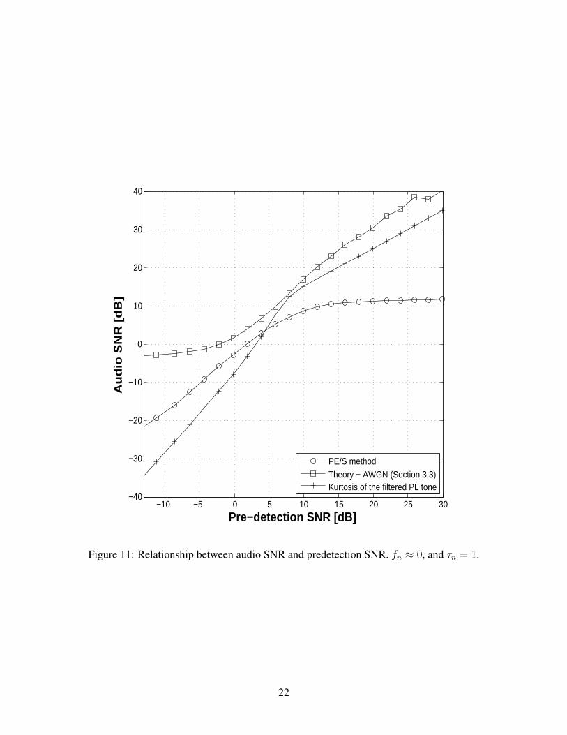
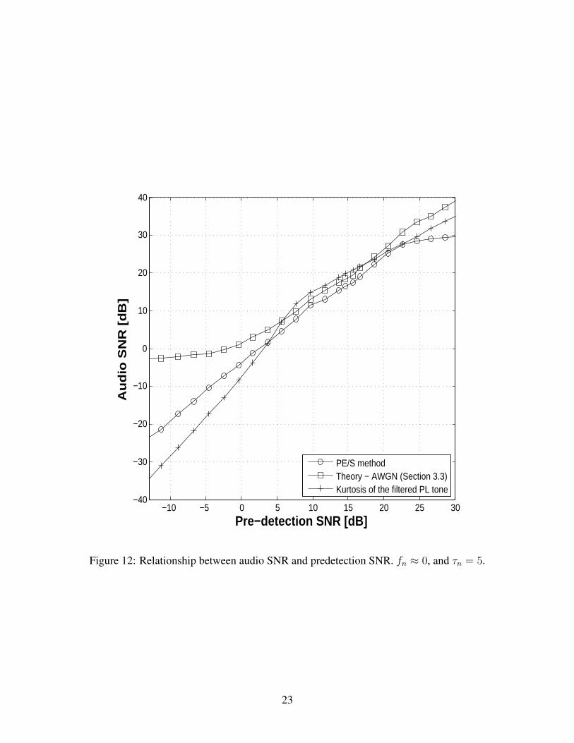
Finally we repeat the test case of Section 4.1.2 but now with a time-varying Rayleigh fading chan-nel. Before equation (4) can be used to simulate the Rayleigh fading environment, the parametersof the Jakes model must be determined. No is set to 16 and the parameter θn is randomly and uni-formly distributed between −π to π. For the following analysis, we coin a term called normalizedDoppler spread, fn = fd/fd,max, where fd is the Doppler spread for a given f and v, and fd,max isthe maximum Doppler spread corresponding to f = 860 MHz and v = 29 m/s. Let τn = τ/τnullrepresent the normalized integration time. Here, τ is the selected integration time for the receivedsignal and τnull = c/(2fv) is the time interval between two consecutive signal nulls.

Consider the best case fading scenario (described in Section 4.1.1) with fn ≈ 0. Figures 10–12 show the audio SNR as a function of predetection SNR using the PE/S method, the kurtosismethod, and the theoretical result (AWGN) for τn = 0.09, 1, and 5 respectively. Now considerthe worst case fading scenario with fn = 1. Figures 13– 15 show the audio SNR as a function ofpredetection SNR using the PE/S method, the kurtosis method, and the theoretical result (AWGNand Rayleigh fading [5]) for τn = 0.93, 9.3, and 93 respectively.

The performance of the PE/S and kurtosis methods for the above cases are summarized in Fig-ure 16. We measured the mean absolute deviation of the PE/S and kurtosis curves from the theo-retical result for a predetection SNR range from 5 dB to 25 dB. It is observed that as the integrationtime is increased from a value much lower than the null-fading period to the null-fading period, thedeviation of the PE/S result from the theoretical result increases by a few dB. However on makingthe integration time much larger than the null-fading period, the deviation actually decreases sig-nificantly since the deep fades get averaged out. Based on the same logic, the kurtosis result alsogets fairly close to theoretical result at higher integration times.

We conclude that although the agreement between the theoretical and simulation results is notvery good, it gets better at sufficiently high values of τn. For a given fn and τn, the disagreementbetween the results can be predicted in a qualitative sense.

4.2 Actual LMR Signals

4.2.1 Control Experiment

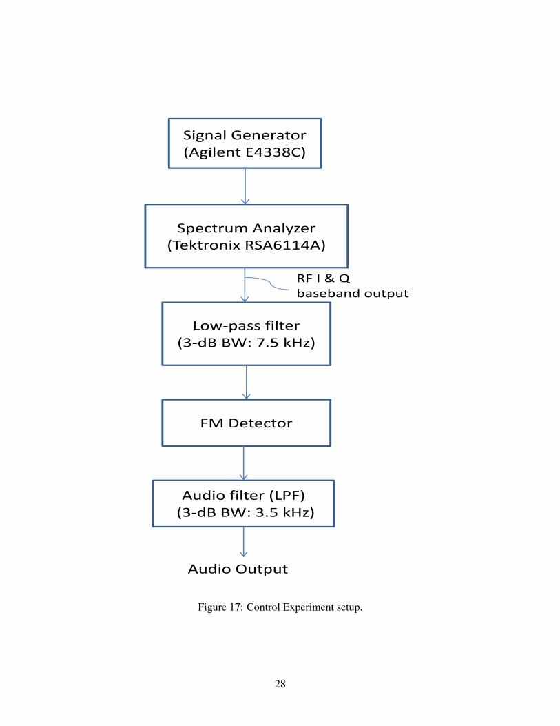
Having tested the two experimental techniques using the simulations, we now compare these meth-ods through a control experiment, where all the system parameters are known and under our con-trol. The experimental setup is shown in Figure 17. We generated an FM signal using AgilentE4438C ESG vector signal generator by modulating a sinusoidal carrier at 453.2 MHz using a123 Hz PL tone (no voice audio). The maximum frequency deviation is set to 4 kHz. The signalgenerator is directly connected to Tektronix RSA6114A spectrum analyzer. The spectrum ana-lyzer has a “RF IQ vs. Time” measurement option. We used this option to record the RF I and

19

Q baseband data to a PC. On the PC, we passed the recorded RF data through a Chebyshev FIRlow-pass filter with 3-dB bandwidth (B/2) set to 7.5 kHz. The order of the filter is 850 taps. Wethen measured the predetection SNR by measuring the total (signal+noise) power when the signalgenerator is on and the noise power when there is no transmission. The filtered RF signal is thendemodulated using a FM detector which is same as in Section ??. The output of the detector ispassed through an audio filter which is a Chebyshev FIR low-pass filter of order 803 taps and with3-dB bandwidth (W ) set to 3.5 kHz. The audio SNR is then measured using the PE/S method. Theexperiment is then repeated for different values of carrier power, to get a predetection SNR rangefrom −12 dB to 35 dB.

Figure 18 shows the resulting plot of the audio SNR as a function of predetection SNR, comparingit to the experimental result. For the experimental result, we have used PE/S method to determinethe audio SNR. Since the transmitter is directly connected to the receiver through a coaxial cable,this ensures that the channel is stationary (fn = 0). It was observed that on increasing the inte-gration time from 50 ms to 100 ms, the audio SNR increased by nearly 1.5 dB. Further increasein integration time from 100 ms to 200 ms resulted in quite small (about 0.2 dB) increase in audioSNR. So increasing integration time beyond 100 ms does not result in significant change in audioSNR. Hence a reasonable integration time would be 100 ms. We observe that the experimentalresult is in close agreement with the simulation (PE/S) result. Since the channel is stationary, wecompare our result to Figure 9 in Section 4.1.2 and find that the results are similar.

We conclude that for a stationary channel both the PE/S and kurtosis methods give quite accurateresults for predetection SNR between 5 dB and 25 dB.

4.2.2 Actual Signals

We now compare these techniques using an actual LMR signal. We recorded an audio signal bytuning our ICOM IC-PCR1500 radio receiver to a local UHF-band police transmission. Figure 19shows the average PSD of the received audio signal. It consists of the message signal and a PL toneat 162.2 Hz. The dynamic spectrum of the captured signal is shown earlier in Figure 1. Figure 20lists the audio SNR computed using PE/S and kurtosis methods for different integration times. Weobserve that increasing the integration time from 50 ms to 100 ms increases the audio SNR byroughly 2 dB. However further increasing the integration time to 200 ms results in a dip of 1 dB.Hence a reasonable integration time for both the methods would be 100 ms. For 100 ms integrationtime, the PE/S and kurtosis methods give audio SNR values as 32.8 dB and 32.7 dB respectively.Referring to Figure 9, we observe that corresponding to our experimental audio SNR value, thesimulation results for PE/S and kurtosis methods are fairly close. Since the experimental audioSNR values using PE/S and kurtosis method are also nearly equal, this proves the correctness ofthe PE/S and kurtosis methods.

20

−10 −5 0 5 10 15 20 25 30−40

−30

−20

−10

0

10

20

30

40


Au

dio

SN

R [d

B]


Figure 10: Relationship between audio SNR and predetection SNR. fn ≈ 0, and τn = 0.09.

21

−10 −5 0 5 10 15 20 25 30−40

−30

−20

−10

0

10

20

30

40


Au

dio

SN

R [

dB

]


Figure 11: Relationship between audio SNR and predetection SNR. fn ≈ 0, and τn = 1.

22

−10 −5 0 5 10 15 20 25 30−40

−30

−20

−10

0

10

20

30

40


Au

dio

SN

R [d

B]


Figure 12: Relationship between audio SNR and predetection SNR. fn ≈ 0, and τn = 5.

23

−15 −10 −5 0 5 10 15 20 25 30

−40

−30

−20

−10

0

10

20

30

40


Aud

io S

NR

[dB

]

PE/S methodTheory − AWGN (Section 3.3)Kurtosis of the filtered PL tone Theory − Rayleigh fading [5]

Figure 13: Relationship between audio SNR and predetection SNR. fn = 1, and τn = 0.93.

24

−15 −10 −5 0 5 10 15 20 25 30−40

−30

−20

−10

0

10

20

30

40


Aud

io S

NR

[dB

]

PE/S methodTheory − AWGN (Section 3.3)Kurtosis of the filtered PL toneTheory − Rayleigh fading [5]

Figure 14: Relationship between audio SNR and predetection SNR. fn = 1, and τn = 9.3.

25

−15 −10 −5 0 5 10 15 20 25 30−40

−30

−20

−10

0

10

20

30


Aud

io S

NR

[dB

]

PE/S methodTheory − AWGN (Section 3.3)Kurtosis of the filtered PL toneTheory − Rayleigh fading [5]

Figure 15: Relationship between audio SNR and predetection SNR. fn = 1, and τn = 93.

26

Doppler shift, normalized to worst case Doppler shift (f = 860 MHz, v = 27 m/s)

Integration time, normalized to the null-fading period (c/2fv)

Mean absolute deviation from the theoretical result (AWGN for fn =0 , Rayleigh fading for fn = 1) for the pre-detection SNR range : 5-25 dB

PE/S Kurtosis

0 0.09 5.32 dB 6.1 dB

1 7.7 dB 4.4 dB

5 2.3 dB 1.65 dB

1 0.93 10 dB 14.6dB

9.3 8.9 dB 13.1 dB

93 6.2 dB 9.81 dB

Figure 16: Effect of different fading characteristics and integration time on the performance ofPE/S and kurtosis methods.

27

Signal Generator

(Agilent E4338C)

Spectrum Analyzer

(Tektronix RSA6114A)

RF I & Q baseband output

Low‐pass filter (3‐dB BW: 7.5 kHz)

FM Detector

Audio filter (LPF) (3‐dB BW: 3.5 kHz)

Audio Output

Figure 17: Control Experiment setup.

28

−10 −5 0 5 10 15 20 25 30 35−20

−10

0

10

20

30

40


Au

dio

SN

R [d

B]

PE/S methodControl experimentKurtosis of the filtered PL tone

Figure 18: Relationship between audio SNR and predetection SNR using simulations and controlexperiment (Non-fading channel).

29

0 500 1000 1500 2000 2500 3000 3500

−90

−80

−70

−60

−50

−40

−30

Frequency [Hz]

Po

we

r S

pe

ctru

m [

dB

pe

r 5

.4 H

z]

PL tone

Figure 13: Power spectrum of the recorded audio signal with integration time of 0.01 s

22

Figure 19: Power spectrum of the recorded audio signal with integration time of 10 ms.

Integration time Audio SNR PE/S method Kurtosis method

50 ms 30.9 dB 30.7 dB 100 ms 32.8 dB 32.7 dB 200 ms 31.6 dB 31.3 dB

Figure 20: Effect of integration time on the performance of PE/S and kurtosis methods as appliedto an actual LMR signal.

30

5 Conclusion

From the simulation studies and experimental results, we conclude that under stationary channelconditions, the PE/S and kurtosis methods are in close agreement with each other for predetectionSNR > 5 dB and integration time ≥ 100 ms. For SNR < 5 dB, PE/S performs better than kurtosismethod. The offset between the two results increases with decreasing predetection SNR, with anasymptotic offset of nearly 14 dB. Under fading conditions, it is observed that as the integrationtime is increased from a value much lower than the null-fading period to the null-fading period, thedeviation of the PE/S and kurtosis results from the theoretical result increases by few dB. Howeveron making the integration time much larger than the null-fading period, the deviation actuallydecreases as the fading behavior get averaged out. In general, at low SNR values, the kurtosisresult flattens out earlier than the PE/S curve. This is because PE/S is statistically optimum whereas kurtosis is not. Hence we conclude that it is possible to estimate FM audio quality from PL toneanalysis over a wide range of conditions.

References

[1] Project web site, “Antenna Systems for Multiband Mobile & Portable Radio.” VirginiaTech., http://www.ece.vt.edu/swe/asmr/.

[2] P. Dent, G. Bottomley, and T. Croft, “Jakes fading model revisited,” Electronics Letters, vol.29, pp. 1162-1163, June 1993.

[3] K. Lee, Coherent Mitigation of Radio Frequency Interference in 10-100 MHz. PhD thesis,Virginia Tech., 2008.

[4] R. Matzner and F. Englberger, “An snr estimation algorithm using fourth-order moments,”in Proc. IEEE International Symposium on Information Theory, p. 119, July 1994.

[5] W. C. Jakes, ed., Microwave Mobile Communications. Piscataway, NJ: IEEE press 1993,ch. 4.

[6] B. R. Davis, “FM Noise with Fading Channels and Diversity”, IEEE Trans. Comm. Tech.,COM-19, No. 6, Part II, December 1971, pp. 1189-1199.

[7] S. O. Rice, “Statistical Properties of a Sine Wave Plus Random Noise,” Bell System Tech. J.27, pp. 109-157, January 1948.

[8] T. S. Rappaport, Wireless Communications: Principles & Practice, Prentice Hall, New Jer-sey, 1996.

31

http://www.ece.vt.edu/swe/asmr/

[9] Telecommunications Industry Association, “TIA Standard: Land Mobile FM or PM – Com-munications Equipment – Measurement and Performance Standards”, TIA-603-C, Decem-ber 2004.

[10] B. Z. Kobb, Wirless Spectrum Finder, McGraw-Hill, 2001.

32

Date post:	19-Apr-2018
Category:	Documents
Upload:	lymien
View:	215 times
Download:	1 times

Characterization of LMR Analog FM Audio Quality … of LMR Analog FM Audio Quality Using PL Tone...

Documents