11TH INTERNATIONAL SYMPOSIUM ON PARTICLE IMAGE VELOCIMETRY - PIV15Santa Barbara, California, September 14-16, 2015

Characterization of the Trilobite Hydrodynamic Particle Separation Microchip withµPIV

E. J. Mossige1,3, A. Jensen1 and M. M. Mielnik2

1 Department of Mathematics, University of Oslo, Oslo, Norway, endrejm@math.uio.no

2 Sintef, Oslo, Norway

3 Trilobite Microsystems, Kristiansand, Norway

ABSTRACT

A hydrodynamic micro particle separator has been tested by means of streakline visualizations and Particle Image Velocimetry (PIV) fordifferent flow configurations. By adjusting the pressure drop and the Reynolds number, it is possible to determine the thickness of a flowlayer that ends up as permeate. The results of the streakline visualizations show that the permeate flow thickness decreases with decreasingpressure drop between the inlet and the permeate outlet. Increasing the Reynolds number has the same effect.

An ensemble averaged PIV method was used to extract the velocity fields from the image data. By visual inspection of the velocity vectorplots, it was found that the location of the stagnation points on the separator separator depend on the Reynolds number.

1. Introduction

Particle separation is important in many applications, ranging from industrial process applications to medical diagnostics. Commonseparation criteria are: size, density, charge, shape and deformability. Combinations of these, such as a combination of size and deformabilityfor particle separation, are also used. Still, size based separation is the most common separation criterion.

For industrial applications, conventional separation methods are most common. These are filtration, sedimentation and centrifugation.Dead-end filters are the most common industrial filters. In a dead-end filter, only particles smaller than the pore size can pass through thefilter. Large particles are collected in the filter, forming a cake that reduces the effective pore size. Eventually, the filter clogs and has to bechanged or cleaned.

In miniaturized systems applications, such as lab-on-a-chip systems, one usually distinguish between discrete and continuous particleseparation[1]. In the former case, particles are separated one by one, whereas in the latter case, they are separated in a continuous manner,enabling e.g. high throughput.

In continuous hydrodynamic separation, also known as passive separation, the separation of particles is performed with no external forcefield to manipulate the migration of particles. Only hydrodynamic forces act on the particles. Therefore, these types of systems have certainadvantages over other types of separation methods, such as electrophoresis and flow cytometry. These advantages include: scalability, highthroughput and ease of implementation on chips for complete micro total analysis systems [1]. Another advantage is integrability into largerprocessing systems with both upstream and downstream processes. Unfortunately, continuous hydrodynamic separation methods sufferfrom low pureness of the processed particle streams and poor handling of liquids with high particle concentrations. Some hydrodynamicseparation technologies, such as microfilters, are also prone to clogging.

Microfilters can be divided into two main types. In the first type the side channels are tangent to the main channel. This is known ascrossflow filtration. The side channel width is either made smaller than the smallest particle in the suspension or large enough to allow forparticles below a threshold dimension to enter [2]. These types of filters are easy to manufacture, but suffer from clogging. To reduce thetendency to clog, [3]suggested a method to increase the shear force tangent to the main channel, at the side channel inlets. In the othertype of microfiltration, one takes advantage of the fact that particles have a tendency to follow the stream which has the highest flow rate,i.e. one takes advantage of the Zweifach-Fung effect[2]. This method was first reported by [4], where they successfully separated polymermicrospheres based on the sphere diameter. In addition, the method was verified for selective enrichment of leukocytes from blood withoutsigns of clogging. This method is now commonly used to concentrate blood samples.

Other passive separation technologies include inertial microfluidics, obstacle induced separation and hydrophoresis[2]. In inertial microfluidics,a force balance on a particle is used to collect particles at lateral positions based on their size. Inertial microfluidics could be used to separate

cells based on their deformability as well as on their size[5]. A separation geometry where in a micropillar array, each row of pillars isshifted laterally compared the upstream one was presented by [6]. Small particles are not subject to any lateral displacement because theyfaithfully follow their initial streamline. Larger particles, on the other hand, migrate laterally because they get associated with streamlinesthat are shifted horizontally compared to their initial streamline. This method is known as obstacle induced separation. It is possibleto move particles by a pressure field induced by three dimensional micro-obstacles, i.e. the obstacle height is smaller than the channelheight. In this micro separation technique known as hydrophoresis, the resulting pressure field generates a transversal flow which movesthe particles to distinct positions. In an article on design principles, [7] found channel width to be the most important geometric parameterfor hydrophoretic performance.

A Trilobite separator is presented in this paper which aims to separate particles based on their size. A large particle generally has differentinertia than a small particle and the hydrodynamic force from the flow on the two particles is therefore generally not the same. In thisarticle, this technique to separate particles is called hydrodynamic particle separation and it is the working principle of the separator.

By the authors’ knowledge, little work is done on analysis of the flow field inside these microseparators. This study uses passive tracerparticles to extract the flow field using an ensemble averaged PIV method.

2. Geometry and Working Principle

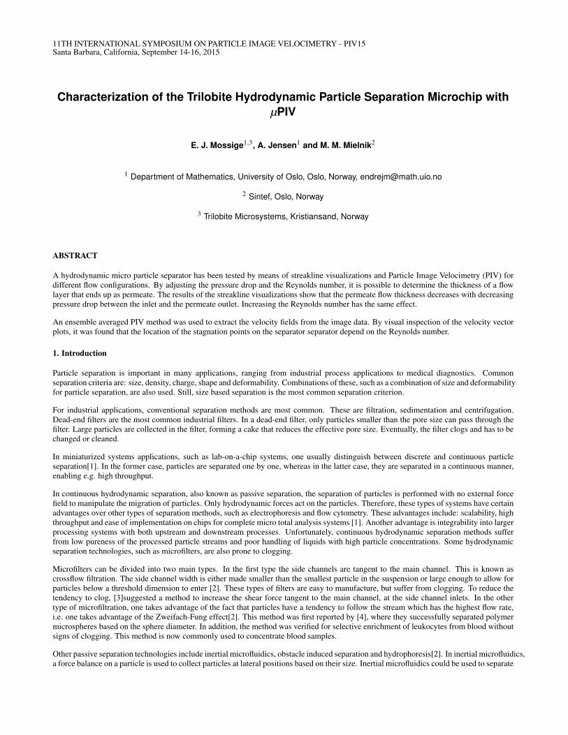
The Trilobite microchip in Figure 1 (a) consists of an inlet, a permeate outlet, and a second outlet downstream interconnected by microfluidicchannels. The trilobite shaped separation unit is located in the center of the main channel. It consists of a bluff body, which serves to guidethe bulk flow of fluid and particles, turbine blade shaped pillars and a permeate outlet. The flow that enters the gaps between the pillars andends up in the oval outlet of Figure 1 (a) is called the permeate flow and has thickness δ, see Figure 1 (b). The pillars serve to guide thepermeate flow onto the permeate outlet.

Now consider a small, spherical, rigid tracer particle with nominal diameter dp and density matched to that of the surrounding fluid.Consider also a larger particle with the same properties except the diameter, Dp>dp. The two particles are subject to the same undisturbed,stationary flow, i.e. the flow field is undisturbed by particles and does not change in time. For low Reynolds number flows, the two particlescannot be separated when they are released from the same position in the flow. This is because they will follow the same streamline ofthe undisturbed flow. Therefore, the Trilobite separator requires Re>1 to separate the two particles described above. When the Reynoldsnumber is sufficiently high, large particles inside the permeate flow layer δ in Figure 1 (b) migrate across the streamlines of the undisturbedflow. If the particle migrate more than a length δ in the wall normal direction, the entire particle is in the accelerated flow region. When theparticle eventually exits through the second outlet downstream, see Figure 1 (a), it has been successfully separated from the small tracerparticle with diameter dp which was released from the same position in the permeate flow. Flow unaffected by the separation unit is denotedas the free flow.

Branching channels, including the calibration channel, guide the flow between inlet, main channel and outlet.

Inlet OutletPermeate Outlet

30 mm

10 mm0.5 mm

1.5 mmBluff body

Pillars

Calibration channel Main channelBranchingchannels

(a) The hydrodynamic particle separation microchip. The trilobite shaped separation unit is located inthe center of the channel. Channel height is 90 µm. Inlet and permeate outlet are pressure regulated.The outlet downstream is an atmospheric pressure outlet.Permeate outlet, pillars and bluff body not to scale.

(b) Working principle of the trilobite shapedseparation unit: Large blue particles can beseparated from the small particles even wheninside δ because they have different inertia.

Figure 1: Illustration and working principle of the microfluidic chip.

3. Experimental Setup and Post Processing

The lab experiments consisted of two parts: calibration of the experimental setup and measurements of the flow around the particleseparator. The microchip seen in Figure 1 was used for both calibration measurements and measurements of the flow around the separator.A schematic of the experimental setup is shown in Figure 2.

A pressure feedback system from Fluigent was used to drive the flow. The pressure system produces a pulseless flow with relative error

less than 0.1%CV. A scale from Mettler Toledo was used to measure the flow rate by sampling the weight at 1Hz and plotting against time.For the measurements of the flow around the separator, inlet and permeate outlet were pressure regulated, and connected to the pressurisedreservoirs. For the calibration, only the inlet reservoir was pressurised and the permeate outlet was plummed. In both cases, the outletdownstream was an atmospheric pressure outlet. To dampen flow transients, a long tubing from the inlet reservoir to the chip inlet wasused. Different lengths were tested to find the required minimum length. The tube inner diameter d was 0.25 mm. Based on the bulkvelocity of the fluid, the kinematic viscosity, and the channel height 2h, the Reynolds number for the calibration measurements was 5.Housing made from PMMA connected the inlet and outlets of the chip to the tubing. Tubing and housing were connected via flangelessfittings from IDEX.

Microscope with CCD camera

Pressure controller and pressurised reservoirs

Pressurised air

Scale with reservoir

Cam

era

Optical ArmBeam Expander

µchip

PC with framegrabberand pressure controllersoftware

Delay Box

Nd:YAG laser

Lase

r 1

Lase

r 2

Input 1

Flash 1

Figure 2: Experimental setup of the PIV system for measurements of the particle separation microchip.

An upright Olympus BX43 microscope with a water immersion objective from Olympus with M=25, NA=1.05 and an adjustible cover glasscorrection between 0 and 0.23 mm was used in the experiments. The cover glass correction was set to 0.17 mm for these experiments. Inorder to avoid a distorted representation of the point spread function associated with an illuminated fluorescent particle, it is advantageousthat the sample medium, in this case water, and the immersion medium of the objective be the same, see e.g. [8]. For the streaklinevisualizations, a dry 10x, NA = 0.25 objective was used.

A double pulsed Litron npiv Nd:YAG laser with built in attenuator and wavelength 532 nm was used as light source. This laser has adouble cavity which enables a short time difference ∆T between two successive pulses. This time difference was set using a delay box. Aninternal time constant inside the delay box marked the lower limit of ∆T. In order for the laser radiance to be stable, it has to be operatedat maximum power. There is a time delay from the when the laser is triggered to the actual lasing, depending on the output power. Thistime delay is 148 µs for Laser 1 and 156 µs for Laser 2 when operated at maximum power. An optical arm from ILA was aligned with thelight source. The optical arm was connected to a custom made microscope connector with adjustible light expanding optics that was alsoconnected to the microscope in the other end. The purpose of the light expander is to expand the laser light beam, whose frontal area isonly 1 mm2, to fill the entire area of the microscope objective. With the pulse width being only 8 ns, any possibility of particle streaks inthe images is removed.

Sequence of laser events:1) Laser 1 is triggered by its internal trigger and sends a trigger signal to the camera and the delay box. Laser 1 pulses after an internal timedelay that depends on the its output power.2) A trigger signal is sent from the flash output of the delay box to the external trigger input on Laser 2. The time delay is set on the delaybox plus an internal time constant is the time delay between the two laser pulses. A Gain Detector from Thorlabs (PDA100A) was used tomeasure the actual time difference ∆T between the two laser pulses. For the calibration measurements and the low velocity measurementsof the separator, ∆T=61.8 µs. For the higher flowrate measurements of the separator, ∆T=20.8 µs.

3) Laser 2 pulses after the internal time delay.

Tracer particles were of type Fluorospheres from Life Technologies with nominal diameter dp equal to 1 µm and with excitation andemission maxima at λex =540nm and λem 560 nm, respectively. These particles were chosen to match well with the wavelength of the laser.Images were captured with a 14bit pco.4000 CCD chip camera, mounted to the microscope with a Nikon F-mount. An efficient way toincrease the signal to noise ratio on a CCD chip is to reduce the amount of background current, which is noise. Therefore, the interlinetransfer CCD chip is cooled to -10◦C. With this camera it is possible to take two images with time difference as low as the time differencebetween the two laser pulses, ∆T . The 9 µm side length of the square pixels makes a good compromise between photon statistics and spatialresolution. When viewed through the 25x-objective, a 1 µm particle is resolved by M ·dp/∆xpixel = 25 · 1µm /(9µm/pixel) = 2.8 pixels.This means that the particle image is sufficiently resolved by the CCD pixels. The particle image diameter de is the diameter of a focusedparticle as observed through a microscope[9]. The diameter of the point-spread function dps f due to diffraction is proportional to M and

λem and inversely proportional to NA, dps f ∝ Mλem/NA. It contributes to de via de =√

d2ps f +d2

g , where dg = Mdp is the geometrical

contribution. For the 25x water immersion objective with NA = 1.05, de ≈ 29.8µm, which in pixels is de,pix ≈ de/∆xpix = 29.8µm/9µm= 3.3 pixels. Because the algorithm to find the interrogation peak uses 3 pixels across the particle diameter, the minimum required particleimage diameter is 3. With de= 3.3, this requirement is fulfilled.

It was of interest to study the flow around the separator with minimal influence from inlets and outlets as well as from side walls. Therefore,the main channel is as much as 30 mm long and 10 mm wide, while the trilobite shaped separation unit is only 1.5 mm long and 0.5 mmwide. From silicon wafers, dry etching was used to etch out the channels and the centered separation unit structures to a depth of 90 µm.

To enhance the wetting abilities of the liquid in the channels, the silicon wavers were oxidized to create a thin hydrophilic siliconedioxide film. A 0.30 mm glass slide is bonded to the chip for sealing and viewing purposes. To withstand the high pressures requiredin hydrodynamic separation, a cover glass thicker than standard 0.17 mm thick cover glass was chosen.

Destilled water at standard conditions was the working fluid in these experiments. Surfactant Triton-X from Sigma Aldrich was added tothe liquid to increase the wetting abilities.

One of the differences between PIV measurements for macroscopic systems and microscopic systems is the influence from particles outsidethe measurement plane for the latter, i.e. the focal plane of the objective. One way to reduce the influence from particles outside the focalplane is to reduce the number of particles in the fluid, see e.g. [10]. To fulfill the requirement that the particles in an interrogation spotbe uniformily distributed[11], one uses averaging techniques, which is a way to syntethically seed the domain with particles. One suchaveraging technique is ensemble averaging, which has advantages over other types of averaging techniques, such as velocity averaging, see[12]. One of the advantages is the reduction of noise, provided that the flow is relatively steady. Another reason is fast convergence of thevelocity field. For these reasons, an in-house made ensemble PIV algorithm was used to extract the velocity fields from the raw image data.A total of 50 image pairs were used in the algorithm to calculate each velocity field.

Window size was 128 pixels and with 75 % overlap, each subwindow ∆x was 32 pixels wide. Each subwindow is therefore 11.5 µm wide,which is the spatial resolution. Therefore, 2 velocity vectors resolve the gap between the pillars.

4. Calibration and Validation

The calibration channel is 500 µm wide, 1500 µm long and 90 µm, see Figure 1. Images were captured in a 400 µm test section halfwaydownstream the calibration channel away from entrence effects, where the flow profile is fully delevoped. When the Reynolds number issufficiently high that the flow has inertia, the characteristic length scales as Re · h, and the entrance length is l ≈ Re ·h/24 [13]. This meansthat the flow is fully developed in the test section for Re up to about 400. Based on the viscosity and density of water at 25◦C, the channelheight and the flow rate, the Reynolds number was 5 for the calibration.

From the channel width, height, kinematic viscosity and the flowrate, the pressure required to overcome the fluidic resistance in therectangular channel was calculated, see [14]. The analytical flow profile is then found by using the pressure drop in an expression for thestreamwise velocity component. The systematic error of the massflow between runs is 1%.

Images were captured in the midplane between the bottom and the top of the channel as well as ±1/6 and ±2/6 channel depths away fromthe midplane. A vertical stepping wheel was used to step between the different planes in the out-of-plane direction with 1 µm resolution.

As the cover lid is 0.30 mm and the objective has cover glass correction for only 0.17 mm, 130 µm of the glass thickness is not correctedfor. Therefore, light rays are refracted at the interface between the different media which normally leads to spherical aberations. Theseaberations result in a distorted representation of the point spread function and the result is that a particle appear elongated in the transversaldirection, see e.g. [8]. The thickness of the slice around the focal plane that contribute to the velocity measurements is commonly referredto as the measurement depth[15]. The measurement depth has contributions from diffraction, geometrical optics and the particle size.Spherical aberations due to unsufficient cover glass correction might lead to an increased measurement depth compared to the case wherethe entire cover glass thickness is corrected for.

y [-

]

-1

-0.8

-0.6

-0.4

-0.2

0

0.2

0.4

0.6

0.8

1

0 0.2 0.4 0.6 0.8 1U [-]

Uana for z = 45 um (middle)Uana for z = 60 umUana for z = 75 umU Measurements for z=45U Measurements for z=60U Measurements for z=30U Measurements for z=75U Measurements for z=15

Figure 3: Streamwise velocities at the midplane, halfway between the channel floor and the glass lid, and at depths 1/6 and 2/6 away fromthe middle. The results show good agreement for planes 1/6 away from the middle. At the midplane, the experiments measure 95% of theanalytical velocity. All velocities are scaled by the maximum of the analytical solution.

The comparison between measured flow profiles and analytical flow profiles is presented in Figure 3. At the midplane, the experimentallymeasured streamwise velocity component is 95% of the analytical velocity. As the flow profile reaches a maximum at the midplane, allcontributions from particles in the out-of-plane direction away from the midplane are negative contributions. This is why the measuredvelocities are lower than the actual flow velocities.

There is a discrepancy between the velocities above and below the midplane; velocities are higher for measurement planes closer to theobjective. This discrepancy is either due the flow profile being asymmetric about the midplane, or it is due to spherical aberations becausethe entire cover glass thickness is not corrected for. From the description of the lab setup and geometry of the calibration channel, asymmetric flow profile seems more likely than an asymmetric one. This leaves spherical aberations as the most likely explanation of thesediscrepancies.

The best match between the analytical solution and the measured velocties is found at ±1/6 channel depths away from the midplane. Incontrast to the midplane velocity measurements, both negative and positive velocity contributions from particles away from the focal planecontribute to these measurements. The negative velocity contributions cancel out the positive velocity contributions and the result is goodagreement between the measured velocities and the actual velocities.

5. Visualization and Measurements of the Flow Field around the Separator

Streakline visualizations obtained using passive tracer particles were performed for low Reynolds number flows as well as for flows withReynolds numbers up to 20. This range of Reynolds numbers was chosen to compare an inertia free or almost inertia free flows with toflows with some influence from inertia.

PIV measurements were performed at middepth at downstream tip of the separator (downstream) and at the side of the separator (upstream).Since the flow is symmetric, measurements were only performed on one side of the structure. Measurements were performed for 2<Re<20and the results for Re = 2 and Re = 20 are presented.

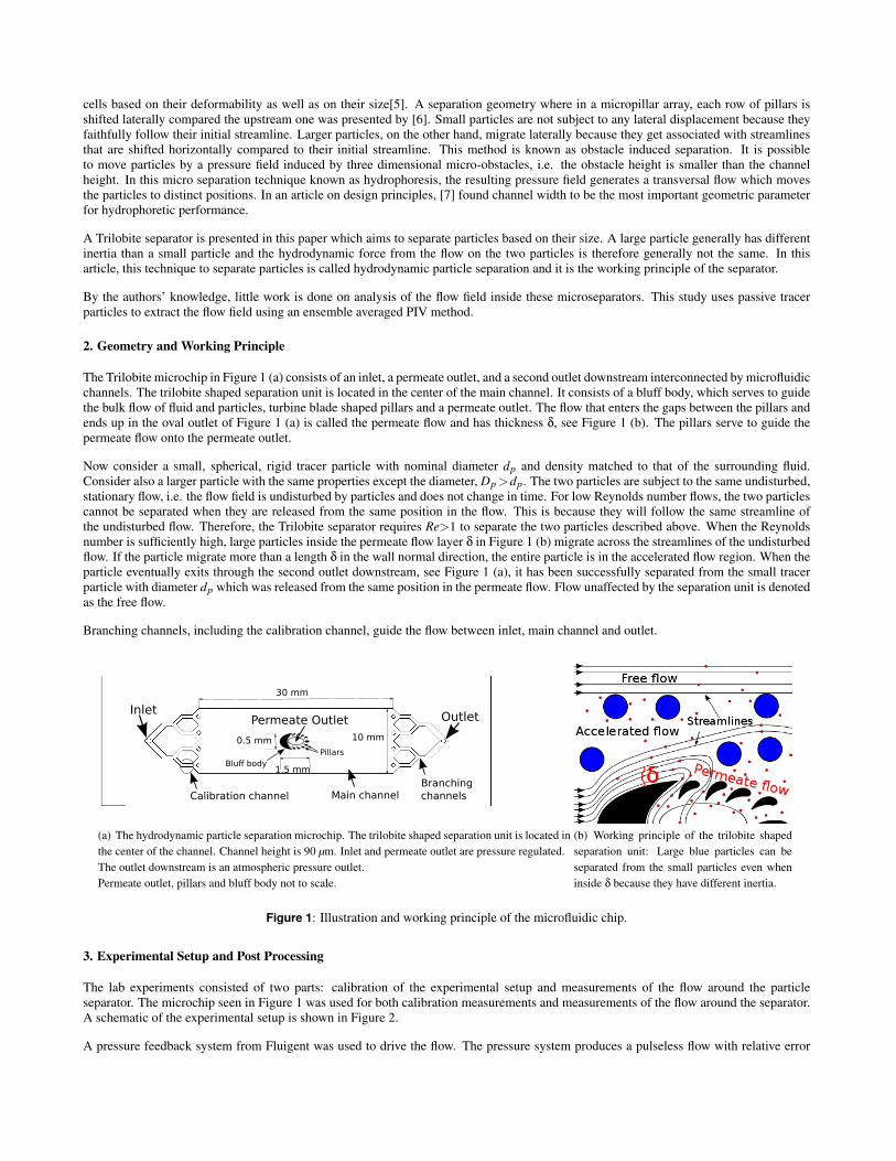
The results of the streakline visualizations show that the separator could be operated in two different modes. For low pressure drop ∆pbetween the inlet and the permeate outlet, the saddle point moves to the downstream tip of the separator. Permeate flow thickness δ thereforedecreases with decreasing pressure drop ∆p. When the pressure drop is increased, the saddle point moves downstream, see Figure 4, and δ

increases. The permeate flow thickness δ is then several times the width of the trilobite shaped separation unit and is larger than the imagewidth. The separator is not able to separate large particles from small particles here because of the strong suction force exerted by thepermeate outlet.

Streakline visualizations show that δ decreases with increasing Re. Therefore, the two tuning parameters that determine δ are ∆p and Re.

(a) Low ∆p results in asaddle point on the downstream tip of the structure. The permeateflow layer thickness δ is about 1/4 of the width of the trilobite shapedseparation unit.

(b) Higher ∆p, results in a saddle point on the right end of the image.

Figure 4: Streaklines obtained using passive tracer particles for Re< 1 show that ∆p could be used to tune the permeate flow. An increasein ∆p results in saddle point that moves downstream and thus a larger δ. Flow is from left to right. Exposure time is 10 seconds.

Velocity vectors from the downstream tip of the separator show the same, yet a more detailed view, as the streakline visualizations in Figure4: the difference between the two operating modes when the separator is operated at low Reynolds number; the saddle point close to thestructure for low ∆P and saddle point farther downstream for higher ∆P, see Figure 5. In the latter case, the strong suction force from thepermeate outlet accelerates the flow in this direction. The saddle point is in this case on the left hand side of the image.

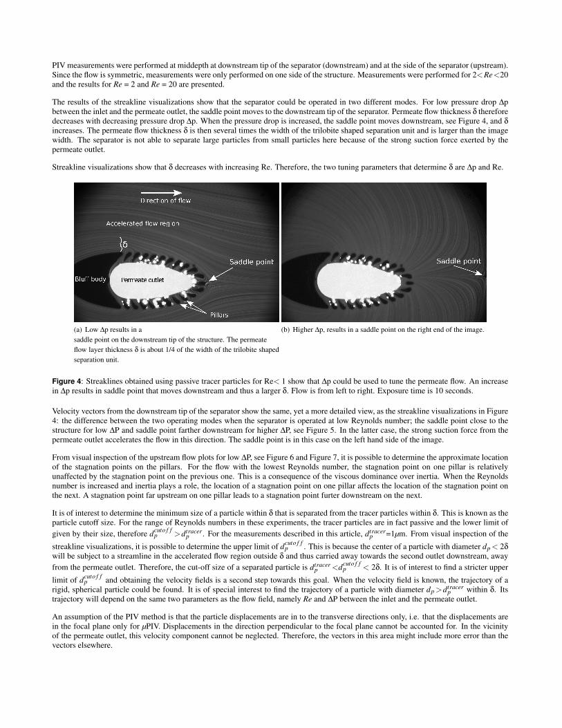
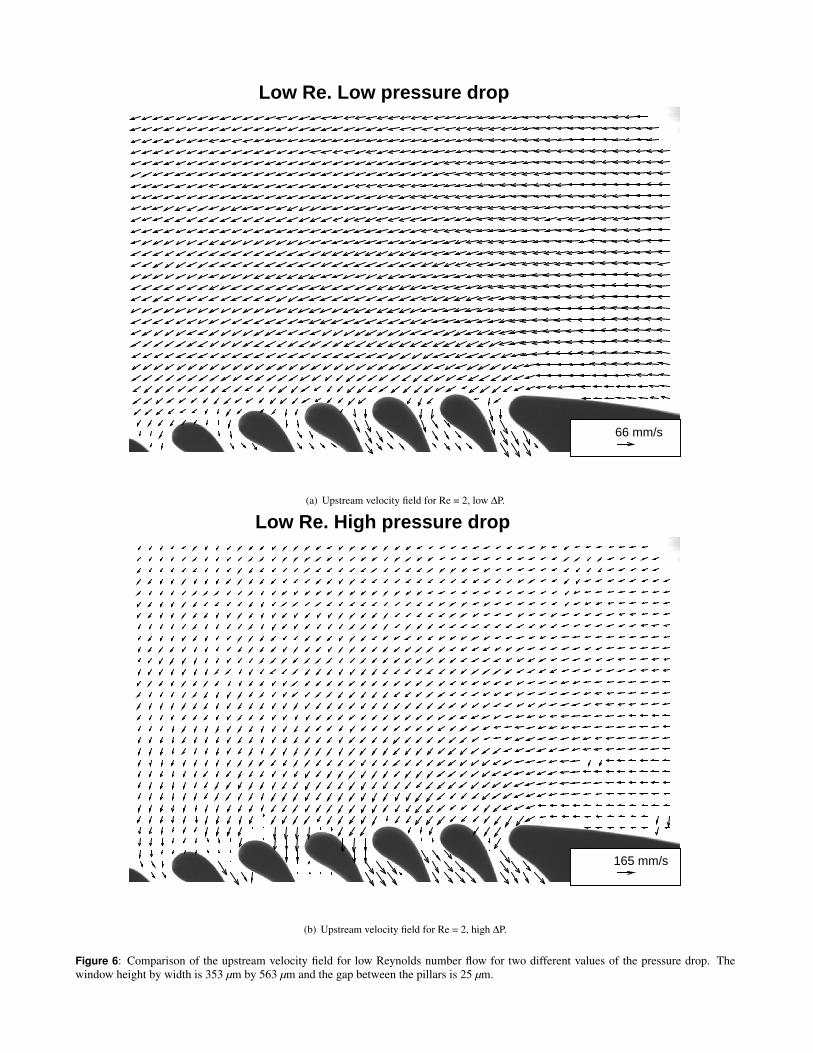
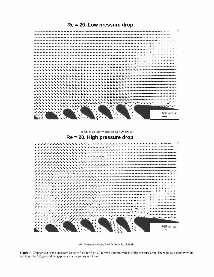
From visual inspection of the upstream flow plots for low ∆P, see Figure 6 and Figure 7, it is possible to determine the approximate locationof the stagnation points on the pillars. For the flow with the lowest Reynolds number, the stagnation point on one pillar is relativelyunaffected by the stagnation point on the previous one. This is a consequence of the viscous dominance over inertia. When the Reynoldsnumber is increased and inertia plays a role, the location of a stagnation point on one pillar affects the location of the stagnation point onthe next. A stagnation point far upstream on one pillar leads to a stagnation point furter downstream on the next.

It is of interest to determine the minimum size of a particle within δ that is separated from the tracer particles within δ. This is known as theparticle cutoff size. For the range of Reynolds numbers in these experiments, the tracer particles are in fact passive and the lower limit ofgiven by their size, therefore dcuto f f

p >dtracerp . For the measurements described in this article, dtracer

p =1µm. From visual inspection of the

streakline visualizations, it is possible to determine the upper limit of dcuto f fp . This is because the center of a particle with diameter dp< 2δ

will be subject to a streamline in the accelerated flow region outside δ and thus carried away towards the second outlet downstream, awayfrom the permeate outlet. Therefore, the cut-off size of a separated particle is dtracer

p <dcuto f fp < 2δ. It is of interest to find a stricter upper

limit of dcuto f fp and obtaining the velocity fields is a second step towards this goal. When the velocity field is known, the trajectory of a

rigid, spherical particle could be found. It is of special interest to find the trajectory of a particle with diameter dp>dtracerp within δ. Its

trajectory will depend on the same two parameters as the flow field, namely Re and ∆P between the inlet and the permeate outlet.

An assumption of the PIV method is that the particle displacements are in to the transverse directions only, i.e. that the displacements arein the focal plane only for µPIV. Displacements in the direction perpendicular to the focal plane cannot be accounted for. In the vicinityof the permeate outlet, this velocity component cannot be neglected. Therefore, the vectors in this area might include more error than thevectors elsewhere.

29 mm/s29 mm/s

Low Re. Low pressure drop

(a) Downstream velocity field for Re = 2, low ∆P.

147 mm/s147 mm/s

Low Re. High pressure drop

(b) Downstream velocity field for Re = 2, high ∆P. Vectors length is doubled to enhance visibility of vectors around the saddle point.

Figure 5: Comparison of the downstream velocity field for low Reynolds number flow for two different values of the pressure drop. Thewindow height by width is 353 µm by 563 µm and the gap between the pillars is 25 µm.

66 mm/s

Low Re. Low pressure drop

(a) Upstream velocity field for Re = 2, low ∆P.

165 mm/s

Low Re. High pressure drop

(b) Upstream velocity field for Re = 2, high ∆P.

Figure 6: Comparison of the upstream velocity field for low Reynolds number flow for two different values of the pressure drop. Thewindow height by width is 353 µm by 563 µm and the gap between the pillars is 25 µm.

406 mm/s

Re = 20. Low pressure drop

(a) Upstream velocity field for Re = 20, low ∆P.

769 mm/s

Re = 20. High pressure drop

(b) Upstream velocity field for Re = 20, high ∆P.

Figure 7: Comparison of the upstream velocity field for Re = 20 for two different values of the pressure drop. The window height by widthis 353 µm by 563 µm and the gap between the pillars is 25 µm.

6. Conclusion

By means of streakline visualizations and PIV measurements the flow field for two different operational modes of the Trilobite separatorwas obtained. The two operational modes of the separator are: saddle point close to the downstream tip of the structure and saddle pointfurther downstream away from the permeate outlet. The saddle point position is determined by ∆P between the inlet and the permeate outletand determines, together with the Reynolds number, the width of the permeate flow layer δ. The cutoff size of a particle to be separatedfrom the smaller tracer particles inside δ could be found from the flow field and should be subject to further work.

7. Acknowledgements

Thanks to Trilobite Microsystems A/S for granting and thanks to the microfluidic lab at the Department for Mathematics at the University ofOslo (UiO) for facilities. Thanks to Johannes Helm at the Department of Molecular Medicine at UiO for letting us use the water immersionobjective. Also, thanks to the Norwegian Research Council and the NORFAB infrastructure project for partial support of fabrication of themicrochannel structures.

REFERENCES

[1] Pamme, Nicole “Continuous flow separations in microfluidic devices” Lab Chip (2007) pp. 1644-1659

[2] Lenshof, Andreas and Laurell, Thomas “Continuous separation of cells and particles in microfluidic systems” Chem. Soc. Rev. (2010)pp. 1203-1217

[3] Mielnik, Michal M. and Ekatpure, Rahul P. and Saetran, Lars R. and Schonfeld, Friedhelm “Sinusoidal crossflow microfiltrationdevice-experimental and computational flowfield analysis” Lab Chip (2005) pp. 897-903

[4] Yamada, Masumi and Seki, Minoru “Hydrodynamic filtration for on-chip particle concentration and classification utilizingmicrofluidics” Lab Chip (2005) pp. 1233-1239

[5] Hur, Soojung Claire and Henderson-MacLennan, Nicole K. and McCabe, Edward R. B. and Di Carlo, Dino “Deformability-based cellclassification and enrichment using inertial microfluidics” Lab Chip (2011) pp. 912-920

[6] Huang, Lotien Richard and Cox, Edward C. and Austin, Robert H. and Sturm, James C. “Continuous Particle Separation ThroughDeterministic Lateral Displacement” Science (2004) pp. 987-990

[7] HSeungjeong Song and Sungyoung Choi “Design rules for size-based cell sorting and sheathless cell focusing by hydrophoresis”Journal of Chromatography A (2013) pp. 191-196

[8] Microscopy U “Water Immersion Objectives” http://www.microscopyu.com/articles/optics/waterimmersionobjectives.html (2015)

[9] Santiago, J. G. and Wereley, S. T. and Meinhart, C. D. and Beebe, D. J. and Adrian, R. J. “A particle image velocimetry system formicrofluidics” Experiments in Fluids (1998) pp. 316-319

[10] Meinhart, C. D. and Wereley, S. T. and Gray, M. H. B. “Volume illumination for two-dimensional particle image velocimetry”Measurement Science and Technology (2000) pp. 809

[11] Sveen, J. Kristian and Cowen, Edwin A. “QUANTITATIVE IMAGING TECHNIQUES AND THEIR APPLICATION TO WAVYFLOWS” In PIV and Water Waves (2004)

[12] Meinhart, C. D. and Wereley, S. T. and Santiago, J. G. “PIV measurements of a microchannel flow” Experiments in Fluids (1999) pp.414-419

[13] Bruus, H. “Acustophoresis” in Short Course 2 at MicroTAS (2013) pp. 40-41

[14] White, Frank M. “Viscous fluid flow” (1991)

[15] C D Meinhart and S T Wereley and M H B Gray “Volume illumination for two-dimensional particle image velocimetry” MeasurementScience and Technology (2000) pp. 809