242
CHARACTERIZATION OF UNBOUND GRANULAR LAYERS IN FLEXIBLE PAVEMENTS RESEARCH REPORT ICAR - 502-3 Sponsored by the Aggregates Foundation for Technology, Research and Education
CHARACTERIZATION OF UNBOUND GRANULAR LAYERS IN FLEXIBLE PAVEMENTS
RESEARCH REPORT ICAR - 502-3
Sponsored by the Aggregates Foundation
for Technology, Research and Education
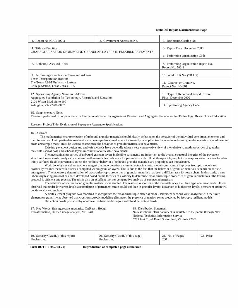
Technical Report Documentation Page
1. Report No.ICAR/502-3
2. Government Accession No.
3. Recipient's Catalog No. 5. Report Date: December 2000
4. Title and Subtitle CHARACTERIZATION OF UNBOUND GRANULAR LAYERS IN FLEXIBLE PAVEMENTS
6. Performing Organization Code 7. Author(s): Alex Adu-Osei
8. Performing Organization Report No. Report No. 502-3 10. Work Unit No. (TRAIS)
9. Performing Organization Name and Address Texas Transportation Institute The Texas A&M University System College Station, Texas 77843-3135
11. Contract or Grant No. Project No. 404001 13. Type of Report and Period Covered Final: December 2000
12. Sponsoring Agency Name and Address Aggregates Foundation for Technology, Research, and Education 2101 Wison Blvd, Suite 100 Arlington, VA 22201-3062
14. Sponsoring Agency Code
15. Supplementary Notes Research performed in cooperation with International Center for Aggregates Research and Aggregates Foundation for Technology, Research, and Education.
Research Project Title: Evaluation of Superpave Aggregate Specifications 16. Abstract The mathematical characterization of unbound granular materials should ideally be based on the behavior of the individual constituent elements and their interaction. Until particulate mechanics are developed to a level where it can easily be applied to characterize unbound granular materials, a nonlinear and cross-anisotropic model must be used to characterize the behavior of granular materials in pavements.
Existing pavement design and analysis methods have generally taken a very conservative view of the relative strength properties of granular materials used as base and subbase layers in conventional flexible pavements.
The mechanical properties of unbound granular layers in flexible pavements are important to the overall structural integrity of the pavement structure. Linear elastic analysis can be used with reasonable confidence for pavements with full depth asphalt layers, but it is inappropriate for unsurfaced or thinly surfaced flexible pavements unless the nonlinear behavior of unbound granular materials are properly taken into account.
Work done by several researchers suggest that incorporating a cross-anisotropic elastic model significantly improves isotropic models and drastically reduces the tensile stresses computed within granular layers. This is due to the fact that the behavior of granular materials depends on particle arrangement. The laboratory determination of cross-anisotropic properties of granular materials has been a difficult task for researchers. In this study, a new laboratory testing protocol has been developed based on the theories of elasticity to determine cross-anisotropic properties of granular materials. The testing protocol is efficient and precise. The test is also an excellent tool for comparative analysis of compacted materials.
The behavior of four unbound granular materials was studied. The resilient responses of the materials obey the Uzan type nonlinear model. It was observed that under low stress levels accumulation of permanent strain could stabilize in granular layers. However, at high stress levels, permanent strain will continuously accumulate.
A finite element program was modified to incorporate the cross-anisotropic material model. Pavement sections were analyzed with the finite element program. It was observed that cross-anisotropic modeling eliminates the presence of tension zones predicted by isotropic resilient models.
Deflection bowls predicted by nonlinear resilient models agree with field deflection bowls. 17. Key Words: fine aggregate angularity, CAR test, Hough Transformation, Unified image analysis, VDG-40,
18. Distribution Statement No restrictions. This document is available to the public through NTIS: National Technical Information Service 5285 Port Royal Road, Springfield, Virginia 22161
19. Security Classif.(of this report) Unclassified
20. Security Classif.(of this page) Unclassified
21. No. of Pages 260
22. Price
Form DOT F 1700.7 (8-72) Reproduction of completed page authorized
CHARACTERIZATION OF UNBOUND GRANULAR LAYERS
IN FLEXIBLE PAVEMENTS
by
Alex Adu-Osei Graduate Research Assistant
Texas A&M University
Report No 502-3
Project No. 404001 Research Report Title: Structural Characteristics of Unbound Aggregate
Bases to Meet AASHTO Design Requirements
Sponsored by Aggregates Foundation for Technology, Research and Education
December 2001
Texas A&M University TEXAS TRANSPORTATION INSTITUTE
College Station, Texas 77840 MS 3135
DISCLAIMER The contents of this report reflect the views of the authors, who are responsible for the facts and the accuracy of the data presented herein. The contents do not necessarily reflect the official views or policies of the International Center for Aggregate Research (ICAR), Texas Transportation Institute (TTI), or Texas A&M University. The report does not constitute a standard, specification, or regulation, nor is it intended for construction, bidding, or permit purposes.
ii
iii
TABLE OF CONTENTS Chapter Page I INTRODUCTION ........................................................................................1 1.1 Problem Statement .................................................................................1 1.2 Objectives...............................................................................................3 1.3 Outline of Dissertation ...........................................................................3 II LITERATURE REVIEW ..............................................................................6 2.1 Characterization of Unbound Granular Materials ..................................7 2.2 Repeated Load Triaxial Testing .............................................................8 2.3 Behavior of Unbound Granular Layers in Pavements ...........................9 2.4 Resilient Behavior Modeling of Unbound Granular Materials ............12 2.4.1 Confining Pressure Model.........................................................15 2.4.2 k-θ Model ..................................................................................16 2.4.3 Uzan Model ...............................................................................16 2.4.4 Lytton Model.............................................................................17 2.4.5 Contour Model ..........................................................................19 2.5 Permanent Deformation Models ..........................................................21 2.5.1 Hyperbolic Model .....................................................................23 2.5.2 VESYS Model...........................................................................24 2.5.3 Exponential/ Log N Model........................................................23 2.5.4 Ohio State University (OSU) Model .........................................25 2.5.5 Texas A&M Model ...................................................................25 2.5.6 Rutting Rate (RR) Model ..........................................................26 2.5.7 Yield Surface Model .................................................................27 2.5.8 Shakedown Model.....................................................................28 2.6 Analysis of Pavements with Unbound Granular Materials ..................29 III DEVELOPMENT OF ANISOTROPIC RESILIENT MODEL AND LABORATORY TESTING.........................................................................31 3.1 Background ..........................................................................................31 3.2 Constitutive Model ...............................................................................36 3.2.1 Orthogonal Planes of Elastic Symmetry ...................................37 3.2.2 Anisotropic Work Potential.......................................................40 3.3 Testing Protocol ...................................................................................41 3.3.1 Triaxial Compression Regime...................................................43 3.3.2 Triaxial Shear Regime...............................................................44
iv
TABLE OF CONTENTS (Cont’d) Chapter Page 3.3.3 Triaxial Extension Regime................................................................45 3.4 System Identification Method ..............................................................46 IV LABORATORY TESTING.........................................................................53 4.1 Equipment ............................................................................................53 4.2 Materials...............................................................................................56 4.3 Sample Size ..........................................................................................58 4.3.1 Stress Distribution in a Cylindrical Sample ..............................62 4.3.2 Preliminary Testing ...................................................................66 4.4 Preparation of Samples.........................................................................68 4.4.1 Compaction Methods ................................................................69 4.4.1.1 Impact Compaction .....................................................69 4.4.1.2 Static Compaction .......................................................70 4.4.1.3 Kneading Compaction.................................................70 4.4.1.4 Vibratory Compaction.................................................70 4.4.1.5 Shear Gyratory Compaction........................................71 4.5 Resilient Testing Protocol ....................................................................74 4.6 Permanent Deformation Testing ..........................................................76 V LABORATORY TEST RESULTS AND ANALYSIS ...............................79 5.1 General ..................................................................................................79 5.2 Resilient.................................................................................................82 5.2.1 Regression Analysis .................................................................106 5.2.2 Compaction Results..................................................................110 5.3 Permanent Deformation ......................................................................115 5.3.1 Accelerated Rutting Parameters ...............................................123 VI DEVELOPMENT OF FINITE ELEMENT PROGRAM...........................127 6.1 Background .........................................................................................127 6.2 Finite Element Formulation ................................................................129 6.3 Pavement Analysis ..............................................................................133 6.3.1 Constitutive Models .................................................................141 6.3.2 Layer Thickness .......................................................................144 6.3.3 Subgrade Modulus....................................................................144 VII FIELD VALIDATION OF RESILIENT RESPONSE...............................147
v
TABLE OF CONTENTS (Cont’d) CHAPTER Page 7.1 Background .........................................................................................147 7.2 Data Analysis ......................................................................................153 VIII CONCLUSIONS AND RECOMMENDATIONS.......................................157 8.1 Conclusions .........................................................................................157 8.2 Recommendations ...............................................................................158 REFERENCES...............................................................................................................161 APPENDIX A TABLES OF AVERAGE RESILIENT STRAIN .............................171 APPENDIX B TABLES OF MODULI AND POISSON’S RATIO ........................195 APPENDIX C VERTICAL AND HORIZONTAL STRESS DISTRIBUTION.............................................................................219
1
CHAPTER I
INTRODUCTION
Pavements are civil engineering structures used for the purpose of carrying
vehicular traffic safely and economically. Since the first hot mixed asphalt was placed
on Pennsylvania Avenue in Washington, D.C., in 1876, flexible pavements have
increased to 94% of the 12.9 million lane kilometers (8 million lane miles) paved roads
in the U.S. (FHWA, 1990).
A conventional flexible pavement consists of a prepared subgrade or foundation
and layers of subbase, base and surface courses (AASHTO 1993). The layers are
selected to spread traffic loads to a level that can be withstood by the subgrade without
failure. The surface course consists of a mixture of mineral aggregates cemented by a
bituminous material. The base and subbase course usually consists of unbound granular
materials. In flexible pavements, and especially for thinly surfaced pavements, the
unbound granular layers serve as major structural components of the pavement system.
1.1 Problem Statement
Existing and past pavement design procedures have generally taken a very
conservative view of the relative strength properties of unbound granular materials.
There has been a recent move towards the use of mechanistic-empirical approaches to
design and analyze pavement structures.
The format of this dissertation follows that of the Journal of Transportation Engineering
of the American Society of Civil Engineers.
2
Conventional flexible pavements have been analyzed as layered elastic systems
resting on a homogeneous semi-infinite half-space. The development of the layered
elastic system solution started when Boussinesq (1885) solved for the stress, strain and
displacement in a semi-infinite linear elastic homogeneous half-space due to a point load
acting on the surface. Burmister (1943) developed a true layered elastic theory for a two-
layer system and extended it to a three-layer system (Burmister, 1945). With the advent
of computers, the theory has been applied to multilayer system with any number of
layers with specified moduli and Poisson’s ratios.
The mechanical properties of unbound granular layers in flexible pavements are
important to the overall structural integrity of the pavement structure. The resilient
(elastic) properties of unbound granular materials are non-linear and stress dependent
(Hicks and Monismith, 1971; Uzan, 1985).
Linear elastic analysis can be used with reasonable confidence for pavements
with full depth asphalt layers, but it is inappropriate for unsurfaced or thinly surfaced
flexible pavements unless the nonlinear behavior of unbound granular materials are
properly taken into account (Brown, 1996). To account for the nonlinear behavior of
unbound granular materials, the layers are usually subdivided into sub-layers to
accommodate variation in resilient modulus caused by the change in stress which occur
with depth as a result of both traffic and overburden loads. There are different sub-
layering methods available for assigning moduli to granular materials. The sub-layering
methods depend on the design method or pavement structure and are totally different
from each other (Wardle et. al., 1998). This multiple layered elastic process can account
for variation in vertical stress but cannot effectively account for variation in lateral or
horizontal stresses. Due to the non-linear behavior of unbound granular materials, and
the variation of vertical and horizontal stresses within a pavement profile, the finite
element method has recently been preferred to analyze pavements over the layered
elastic method (Brown, 1996).
Due to the large amount of computer time and storage required of most finite
element method programs, they have been used primarily for research analysis instead of
3
routine design. With the advent of faster and larger memory computers, it has become
possible to use finite element method programs to analyze pavements on personal
computers.
One of the problems encountered by researchers developing finite element
method programs for pavement systems with compacted unbound granular materials
concerns the tendency for horizontal stresses to be computed in the granular layers.
Since unbound granular materials have negligible tensile strength aside from that
induced by suction and particle interlock, adjustments are usually applied to avoid
predicting false failure conditions in the granular layers (Brown, 1996).
Recent developments in pavement materials research suggest that directional or
anisotropic elastic modeling can reduce and even reverse horizontal tensile stresses
predicted in unbound granular layers with isotropic elastic properties (Tutumluer, 1995).
However, the determination of cross-anisotropic elastic properties using a conventional
triaxial setup is difficult.
1.2 Objectives
The main objectives of this study are to:
• identify and assess the most accurate models used to characterize unbound granular
layers which can be effectively incorporated into a layered (non-linear) elastic or
finite element model
• develop improved characterization protocols and models to provide a more accurate
assessment of the contribution of unbound granular layers to the overall structural
integrity of flexible pavements
• evaluate the revised characterization model to aggregate variables through a
laboratory study and assess the impact of these variables on performance.
1.3 Outline of Dissertation
This dissertation consists of eight chapters. An extensive literature survey on the
characterization of unbound granular materials is included in Chapter II. The literature
review summarizes existing laboratory, analysis, resilient modeling and permanent
4
deformation modeling used to characterize the behavior of unbound granular materials in
flexible pavements. Based on the findings of the literature review, nonlinear cross-
anisotropic resilient modeling was identified to be the best available model to
characterize granular materials.
The development of a new laboratory testing protocol to determine the nonlinear
cross-anisotropic resilient response of unbound granular materials is presented in
Chapter III. The testing protocol involves applying dynamic stress regimes within static
stress levels and measuring material response (strains). The measured strains are used as
input into a system identification method to determine five stress dependent cross-
anisotropic properties of unbound granular materials.
A comprehensive laboratory test matrix was developed to study the resilient and
permanent deformation behavior of four granular materials. Chapter IV includes
description of the laboratory characterization phase of this study. The laboratory test
results are presented and discussed in Chapter V. The effect of moisture, gradation, and
material type on the deformational response of granular materials are also discussed.
A finite element program was modified to include cross-anisotropic material
modeling in pavement layers. Chapter VI contains the development and modifications
made to the finite element program. The finite element program was used to analyze
resilient pavement response for 27 different pavement sections. Pavement response in
the form of stress distributions was obtained for different material models. Chapter VI
also discusses the pavement sections analyzed and evaluates the effect of different
material models on the distribution of stresses within the pavement sections.
Chapter VII presents field validation of the resilient response. The pavement
sections and data collection methods are detailed in this chapter. Falling Weight
Deflectometer and Multi-Depth Deflectometer data were used to backcalculate material
properties of two pavement sections. Comparisons were made between field deflection
bowls and deflection bowls predicted by different material models using the finite
element program.

5
The major findings of this research are outlined in Chapter VIII.
Recommendations are also made in this chapter for future research.
6
CHAPTER II
LITERATURE REVIEW
Unbound granular materials are multi-phase materials comprised of aggregate
particles, air voids and water. The mathematical characterization of unbound granular
materials should ideally be based on the behavior of the individual constituent elements
and their interaction. This calls for the use of particulate mechanics techniques to
characterize the behavior of unbound granular materials. However, such an approach can
be rather complex and would not be particularly suitable in pavement engineering
applications. As faster computers become available, particulate mechanics becomes a
more suitable means to characterize the behavior of unbound granular materials. Also,
since the scale of practical interest is in the range of tens to hundreds of feet, the
microscopic effects of unbound granular materials can be averaged and treated as a
continuum (Chen and Mizuno, 1990).
The mechanical behavior of unbound granular materials, like soils, is influenced
by factors such as density, stress history, void ratio, temperature, time, and pore water
pressure. It is difficult to adequately incorporate these factors in a simple mathematical
model and then to implement the model realistically into a computer-based numerical
analysis, within the framework of continuum mechanics.
Existing pavement design and analysis methods rely on empirical procedures
developed through long-term experience with specific types of pavement structure and a
limited number of types of pavement construction material under limited conditions.
These empirical methods have generally taken a very conservative view of the relative
strength properties of granular materials used as base and subbase layers in conventional
flexible pavements.
Use of empirical models should be limited to the conditions on which they are
based and cannot usually account for changes in loading and environmental conditions.
There has been a recent emphasis on the use of mechanistic-empirical approaches to
design and analyze pavement structures. In mechanistic-empirical procedures, models
7
based on physics and engineering principles are used to predict pavement response. This
is adjusted, or calibrated, to fit observed performance, or empirical data. Understanding
the behavior of pavement materials and their accurate characterization are important to
the successful implementation of any mechanistic-empirical procedure.
2.1 Characterization of Unbound Granular Materials
The purpose of laboratory methods is to subject a representative pavement
material sample to an environment (consisting of simulated traffic loading and
environmental conditioning) that closely simulates field conditions. The general stress
regime experienced by an element of material within a pavement structure as a result of
a moving wheel load on the surface consists of pulses of vertical and horizontal stresses
accompanied by a double pulse of shear stress. Also, the principal stresses in an element
of pavement material rotate with the approach and departure of a wheel load (Lekarp et
al., 2000).
Laboratory testing equipment must be capable of applying a load which
accurately simulates the effects of traffic. For pavements, this could demand complex
facilities. However, laboratory testing methods must also be simple and repeatable
enough so that highway agencies can perform them routinely and quickly acquire
necessary material parameters.
It has been reported that a close match to field conditions can be obtained by the
use of a Hollow Cylinder Apparatus (Alavi, 1992, Chan et al 1994), with which the
rotation of principal stresses can be accommodated. The use of a Hollow Cylinder
Apparatus (HCA) is complex and has only been used for research. However, simpler
testing protocols exist which involve the use of stress invariants and which express stress
regimes in terms of octahedral shear and normal stresses (Brown, 1996). The invariant
approach has been applied in conjunction with repeated load triaxial testing to
characterize the response of granular materials in recent years. The deformation of
unbound granular materials under repeated traffic loading is defined by a resilient
response which is important for the load carrying ability of the pavement and a
8
permanent strain response, which characterizes rutting and long-term pavement
deformation (Lekarp et. al., 2000).
Granular material base and subbase layers are generally partially saturated in
pavements. Varying the moisture regime in laboratory triaxial test specimens is
straightforward, and the effects of moisture changes on material response parameters can
be easily measured. Appropriate models can be constructed from the results. Pappin et.
al. (1992) showed that the resilient response modeled for dry granular material is equally
applicable to saturated and partially saturated conditions, provided the principle of
effective stress is observed. In practice, although laboratory modeling of moisture
effects is readily accomplished, estimation of the effective stress state in a pavement
granular layer in the field may not be straightforward (Brown, 1996).
2.2 Repeated Load Triaxial Testing
The study of the mechanical properties of unbound granular materials calls for a
test in which principal stresses and strains that span the range of expected conditions can
be evaluated so that extrapolations used by structural models are kept to a minimum. The
most convenient standard test, which allows for the direct measurement of principal
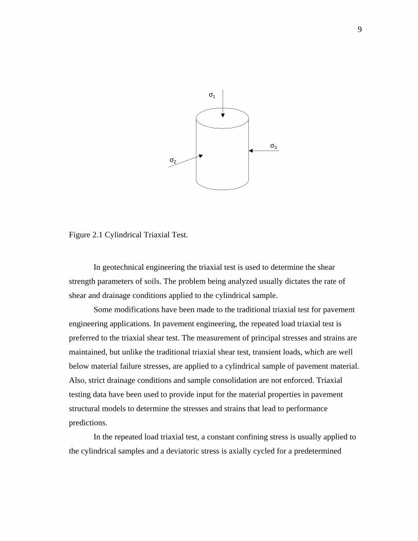
stresses and strains, is the cylindrical triaxial test (Figure 2.1). The shape of the sample
required is simple and practical for both field representation and easy laboratory
preparation. The minor principal stress, σ3, and intermediate principal stress, σ2, are
equal to the confining stress applied to the sample. The triaxial test has been used with
notable success in the field of geotechnical engineering and its principles have been
extended to the field of pavement engineering.
9
σ1
σ3
σ2
Figure 2.1 Cylindrical Triaxial Test.
In geotechnical engineering the triaxial test is used to determine the shear
strength parameters of soils. The problem being analyzed usually dictates the rate of
shear and drainage conditions applied to the cylindrical sample.
Some modifications have been made to the traditional triaxial test for pavement
engineering applications. In pavement engineering, the repeated load triaxial test is
preferred to the triaxial shear test. The measurement of principal stresses and strains are
maintained, but unlike the traditional triaxial shear test, transient loads, which are well
below material failure stresses, are applied to a cylindrical sample of pavement material.
Also, strict drainage conditions and sample consolidation are not enforced. Triaxial
testing data have been used to provide input for the material properties in pavement
structural models to determine the stresses and strains that lead to performance
predictions.
In the repeated load triaxial test, a constant confining stress is usually applied to
the cylindrical samples and a deviatoric stress is axially cycled for a predetermined
10
number of times. Allen (1973) used variable confining stresses and reported higher
values of Poisson’s ratio compared to the constant confining stress.
The transient loads are chosen so that they best represent typical stress conditions
within a pavement. Charts are available that can be used to select the cycle of a transient
load (Barksdale, 1971). A typical transient load consists of a 1.0-second cycle sinusoidal
load consisting of 0.1-second load duration and a 0.9-second rest. This load cycle was
established to simulate the application of traffic loads on the pavement (Barksdale,
1971).
The repeated load triaxial test has been used extensively to study the behavior of
unbound granular materials, despite its inability to simulate the rotation of principal
stresses associated with shear stress reversal under a rolling wheel load. Allen (1973)
conducted triaxial tests in which the chamber confining pressure was varied
simultaneously with the deviator stress. While the technique did not account for the
rotation of principal planes, it attempted to better simulate conditions under a moving
wheel load. Stress pulse duration was 0.15 seconds for the primary test series. Results
of the variable confining pressure tests yielded slightly lower values of the resilient
modulus than did the constant confining pressure tests. However, the difference was not
constant and did not appear to be significant. Using a Hollow Cylinder Apparatus
(HCA), Chan (1990) demonstrated that resilient strains were unaffected by the rotation
of principal stress phenomenon. He also showed that the principal planes of strain
remained coincident with those of stress. These findings support the use of an invariant
approach for pavement analysis and the use of relatively simple resilient strain models
derived from triaxial tests rather than a more complex apparatus such as the HCA.
There has been extensive work in the development of the repeated load triaxial test
in both Europe and North America. The test has been used in the U.S. since the 1950's
(Seed et al., 1955). The American Association of State Highway and Transportation
Officials (AASHTO) have adopted three procedures for measuring the resilient modulus
of granular materials in the past. The recent AASHTO standard procedure (AASHTO
T294-94; “Resilient Modulus of Unbound Granular Base/Subbase Materials and
11
Subgrade Soils” - SHRP Protocol P46) includes method for measuring axial
deformations on the specimen using externally mounted Linear Variable Differential
Transducers (LVDTs). The procedure does not provide methods for measuring the
lateral/radial strains. Also, confining stresses are not cycled and only deviator stresses
are cycled.
Other researchers (Nazarian, 1996 and Tutumluer, 1998) have recommended
changes to AASHTO T-294-94 to include measurement of lateral strains and specimen
conditioning. In Europe, a triaxial apparatus was developed at Nottingham University
(Boyce 1976) which has a system for cycling both deviator and confining stresses. Pore
water pressure is also measured during the test. Details of the Nottingham apparatus are
outlined in Boyce (1976), Pappin (1979), Boyce et. al. (1976), and Brown et. al. (1989).
It can be seen that a single testing protocol has not been universally adopted.
For pavement applications the strains measured in a repeated load triaxial test are
separated into elastic or resilient part, for resilient modulus, and a plastic part, for
permanent deformation (Lekarp et. al., 2000).
2.3 Behavior of Unbound Granular Layers in Pavements
Consolidation, distortion and attrition occur when a granular material deforms
under load (Lekarp, et. al. 2000). The response of an element of granular material in a
pavement depends on its stress history, the current stress level, and the degree of
saturation. Granular materials are not elastic but experience some non-recoverable
deformation after each load application. In the case of transient loads, and after the first
few load applications, the increment of non-recoverable deformation is much smaller
compared to the increment of resilient/recoverable deformation. This resilient behavior
of granular layers is the main justification for using elastic theory to analyze their
response to traffic loads (Brown, 1996). The engineering parameter generally used to
characterize this behavior is resilient modulus (MR). The resilient modulus is obtained
from repeated load triaxial tests, and it is calculated based on the axial recoverable strain
under repeated axial loads.
12
The nonlinear stress-strain relationship of unbound aggregates at strain levels
existing in pavements has been represented through the application of stress-dependent
models of the resilient modulus and Poisson’s ratio. The factors affecting the resilient
modulus and Poisson’s ratio have been studied by many researchers including Hicks
(1970), Hicks and Monismith (1971), Allen (1973), Uzan (1985), Barksdale and Itani
(1989) and Sweere (1990). Factors identified to influence the resilient modulus and
Poisson’s ratio of unbound granular materials include stress levels, density, gradation,
moisture, stress history, aggregate type and particle shape. Lekarp et. al (2000) provided
an extensive literature review on resilient modeling and factors affecting the resilient
properties of unbound granular materials. Although researchers seem to agree on the
influence of stress and moisture on modulus, there are conflicting reports on the other
factors.
Moduli variations due to moisture changes can be quantified in the laboratory.
Anticipated seasonal variations in moisture content of granular layers must be included
in the design process, so that appropriate laboratory derived model can be used properly.
The term “resilient” has a precise meaning. It refers to that portion of the energy
that is put into a material while it is being loaded that is completely recovered when it is
unloaded. As noted in the SHRP A-005 project (Report A357), the Poisson’s ratio of a
resilient material is also stress dependent and is tied to the same material constants as the
resilient modulus. The importance of this fact is that immediately beneath a tire load, an
unbound aggregate generates its own lateral confining pressure and becomes very stiff,
almost as if it were forming a moving vertical column that travels along immediately
beneath the load (Lytton, 1998). How large the confining pressure and how stiff the
aggregate base becomes depend strongly upon how large the Poisson’s ratio becomes.
Contrary to linear elastic materials in which the Poisson’s ratio cannot rise above 0.5, in
unbound aggregate bases, the Poisson’s ratio has been measured in the laboratory and
the field to be above 0.5 (Allen, 1973). This is possible because both the resilient
modulus and the Poisson’s ratio depend upon the stress level instead of being
independent of it as in a linearly elastic material.
13
A Poisson’s ratio of 0.5 means that when a load is applied to a material it may
change in shape but not in volume. A Poisson’s ratio less than 0.5 mean that when a
material is loaded in compression, it may change in shape but it also decreases in volume
(consolidation). A Poisson’s ratio larger than 0.5 means that the material may change in
shape, but it will also increase in volume (dilate). It is this tendency to increase in
volume under load, dilatancy, which makes unbound granular base layers so useful in a
pavement structure (Lytton, 1998). When a collection of particles (aggregate) is loaded,
the individual particles will try to wedge or rotate past the other particles. If the particles
have been well compacted, this wedging and rotating action will force the particle apart,
causing the overall volume to change.
This volume change will occur even if all of the particles are spheres, that is ,
perfectly round (Lytton, 1998). A different amount of volume change will occur if the
particles are oblong or flat or plate shaped. Naturally, if the volume change depends
upon the shape of the particles, then the Poisson’s ratio depends on their shape.
Similarly, the range and distribution of the individual particle sizes also affect what the
Poisson’s ratio will be under different states of stress (Lytton, 1998). The impact of
particle shape and gradation on the Poisson’s ratio and the effect of the Poisson’s ratio
on the performance of unbound aggregates in a pavement under load should be
accommodated by granular material constitutive models in mechanistic pavement
design.
Unbound granular materials like most geologic materials exhibit anisotropic
behavior. During compaction, some anisotropy is induced in the granular layers before
traffic loads impose further anisotropy. After incorporating anisotropic elastic modeling
in the GT-PAVE finite element code, Tutumluer (1995) reported that cross-anisotropic
elastic modeling can predict the behavior of unbound granular layers better than
isotropic elastic model. The significance of this directional-dependent nature of the
modulus and Poisson’s ratio will be discussed in detail later.
14
2.4 Resilient Behavior Modeling of Unbound Granular Materials
Resilient response of unbound granular materials is usually characterized by
resilient modulus and Poisson’s ratio or by shear and bulk modulus. For repeated load
triaxial tests with constant confining stress, the resilient modulus and Poisson’s ratio are
defined as (Lekarp et. al., 2000):
1
31 )(ε
σσ∆ −=RM (2.1)
1
3εεν −= (2.2)
where;
MR = Resilient modulus,
ν = Resilient Poisson’s ratio,
σ1 = Major principal or axial stress,
σ3 = Minor principal or confining stress,
ε1 = Major principal or axial resilient strain, and
ε3 = Minor principal or radial resilient strain.
For repeated load triaxial test with variable confining stress, resilient modulus
and Poisson’s ratio are defined as (Lekarp et. al., 2000):
33311
31312)(
)2()(σ∆εσσ∆ε
σσ∆σσ∆−+
+−=RM (2.3)
)(2 31133
1131σσ∆εεσ∆
εσ∆εσ∆ν+−
−= (2.4)
Many researchers have used laboratory data to model the nonlinear stress-
dependence of resilient modulus and Poisson’s ratio. The following discussion of
selected models is intended to highlight the importance of stress levels to describe the
resilient behavior of unbound granular materials.
15
2.4.1 Confining Pressure Model
Seed et al., (1967) subjected sand and gravel, both saturated and dry, to repeated
load triaxial testing and expressed the results in the form:
231k
R kM σ= (2.5)
where k1 and k2 are regression constants. They used Equation 2.5 with success to predict
the deflections in prototype pavements.
2.4.2 k-θ Model
A practical nonlinear description of the resilient modulus of unbound granular
materials was reported by Hicks and Monismith (1971) and implemented in the
AASHTO Guide for the Design of Pavement Structures. The resilient modulus was
described as depending upon the sum of the principal stresses (Equation 2.6).
21k
R kM θ= (2.6)
where θ = sum of principal stresses or first stress invariant (σ1 + 2σ3).
Equation 2.6 has become the most common representation of the resilient
modulus, relating effects of the state of stress to layer stiffness for use in pavement
design. Allen (1973) compared the results from constant confining pressure triaxial tests
with those from variable confining pressure tests. Similar results were obtained from
each test type, although constant confining pressure conditions yielded higher values for
Poisson’s ratio. The data showed that Equation 2.6 fit the data better than Equation 2.5.
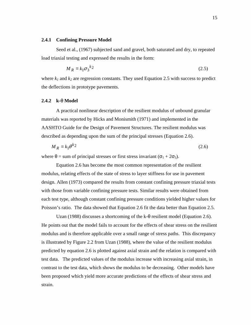
Uzan (1988) discusses a shortcoming of the k-θ resilient model (Equation 2.6).
He points out that the model fails to account for the effects of shear stress on the resilient
modulus and is therefore applicable over a small range of stress paths. This discrepancy
is illustrated by Figure 2.2 from Uzan (1988), where the value of the resilient modulus
predicted by equation 2.6 is plotted against axial strain and the relation is compared with
test data. The predicted values of the modulus increase with increasing axial strain, in
contrast to the test data, which shows the modulus to be decreasing. Other models have
been proposed which yield more accurate predictions of the effects of shear stress and
strain.
16
Figure 2.2 Test Results versus Modulus/Strain Relation from Equation 2.6 [after Uzan
(1988)].
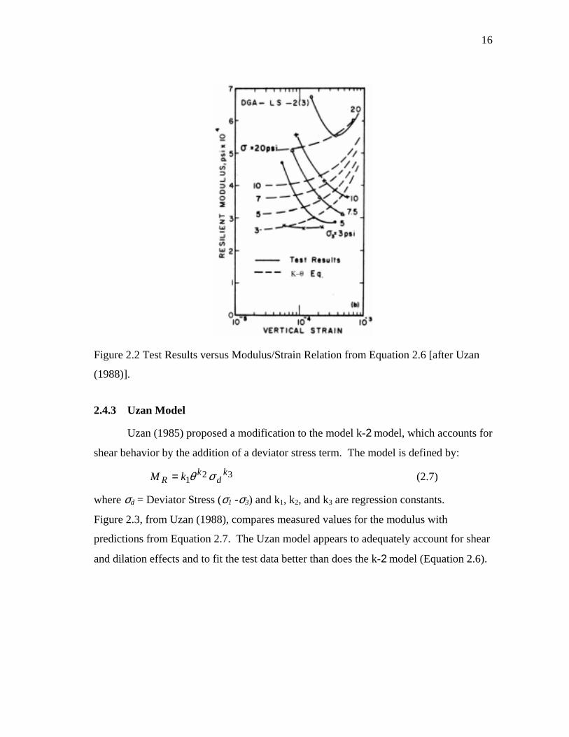
2.4.3 Uzan Model
Uzan (1985) proposed a modification to the model k-2 model, which accounts for
shear behavior by the addition of a deviator stress term. The model is defined by:
321k
dk
R kM σθ= (2.7)
where σd = Deviator Stress (σ1 -σ3) and k1, k2, and k3 are regression constants.
Figure 2.3, from Uzan (1988), compares measured values for the modulus with
predictions from Equation 2.7. The Uzan model appears to adequately account for shear
and dilation effects and to fit the test data better than does the k-2 model (Equation 2.6).
17
Figure 2.3 Experimental Results Compared to Uzan Model. [After Uzan (1988)].
Witczak and Uzan (1988) modified Equation 2.7 by replacing the deviator stress
term with octahedral shear stress and non-dimensionalized the model (Equation 2.8) to
facilitate easy conversion between different units. The Uzan model has been accepted as
a universal material model for pavement materials and has become popular in routine
pavement analysis.
331
1
k
a
octk
aaR PP
IPkM
=
τ (2.8)
where;
I1= First stress invariant (sum of principal stresses),
τoct = Octahedral shear stress, and
Pa = Atmospheric pressure.
18
2.4.4 Lytton Model
Lytton (1995) argues that unbound granular materials in pavements are normally
unsaturated and applied the principles of unsaturated soil mechanics to the Uzan model.
To determine the effective resilient properties of unsaturated granular materials Lytton
(1995) added a suction term to the Uzan model and expressed the resilient modulus as:
3241
132
11
33 k
a
octk
aaR
k
a
octk
a
maR PP
kIPkMorPP
fhIPkM
−=
−=
ττθ
(2.9)
where
θ = Volumetric water content,
hm = matric suction,
f = function of the volumetric water content, and
k4 = θ fhm .
2.4.5 Contour Model
The nonlinear stress-strain behavior of unbound granular materials have also
been modeled by decomposing both stresses and strains into volumetric and shear
components (Boyce, 1976). Brown and Papin (1981) modified the contour model
originally developed by Boyce (1976) to account for stress path effects. The model uses
bulk and shear moduli to describe material properties. Equations 2.10, 2.11, and 2.12
are used to calculate volumetric and shear strains.
1
2111 11 I
PPI
K o
dk
oiv
−
=
− σβε (2.10)
d
k
oiq P
IG
σε12
13
1−
= (2.11)
311
12
11
12
22
123
1 kdk
o
dk
oiq l
IPI
IPI
G
−
=
σσε∆ (2.12)
19
where
Ki and Gi are initial bulk and shear moduli,
I1 = σ1 + σ2 + σ3,
σd = σ1 -σ3,
po = reference pressure,
I11, σd1 and I12, σd2 are I1 and σd at stress states 1 and 2 respectively,
1 = (∆I12 + ∆σd
2)½, and
β, k1, k2 , and k3 are statistical material constants. This model yields accurate
values for the resilient modulus over a wide range of stress paths. However, since the
model requires determination of four material constants, laboratory and analytical
procedures may be too complicated for routine design use (Tutumluer, 1995). Other
models based on the contour models have also been proposed (Jouve et al., 1987; Thom,
1988; Sweere, 1990).
A review of the literature reveals that while the Uzan type of model is highly
favored in the U.S., the bulk and shear moduli models are popular in Europe.
The resilient Poisson’s ratio has also been modeled to depend on stress levels by
a few researchers. Hicks and Monismith (1971) observed that the resilient Poisson’s
ratio increases with decreasing confining pressure and used a third-order polynomial to
describe resilient Poisson ratio (Equation 2.13).
3
3
12
3
1
3
1
+
+
+=
σσ
σσ
σσν DCBA (2.13)
where A, B, C and D are regression coefficients.
Lytton et al. (1993) derived a partial differential equation based on
thermodynamic principles to relate the resilient Poisson’s ratio with stress (Equation
2.14).
+−+
+=
∂∂+
∂∂
21
2/2
321
2/2
3
11/2
61
311
32
I
k
J
k
I
k
J
kIIJ
ννν (2.14)
20
where
J2/ is second stress invariant of the deviatoric stress tensor, and
Ki are the regression coefficients from the Uzan model.
The solution to this partial differential equation led to two more regression coefficients
including the three coefficients from the Uzan model. This model was termed the k1-k5
model. There are infinite number of solutions to this partial differential equation. Lytton
et al. observed from laboratory data that for pavement materials, the particular solution
can be expressed as:
−++
+−+−
−
+−=+
/3
/3
2/3
/3
/3
22/
322
2
/332/
32514 ,2
1,2
)3(2
3)( kkkBkkkkBk
yx
yxyxuk vvk
k
kkkkkkν
(2.15)
where
x = I1,
y = J2/ ,
u1 = 3y-x2,
Bv(c,d) is the incomplete Beta function,
K3/ = k3 / 2,
k1, k2, k3 are regression coefficients determined from the Uzan model, and
k4, k5 are new regression coefficients.
2.5 Permanent Deformation Models
Resilience characteristics of paving materials are most important in fatigue
cracking analyses. However, predictive procedures for rutting in flexible pavements
require the assessment of the permanent deformation potential of granular layers.
Energy is put into a material when it is loaded. The resilient energy is that part of
the applied energy that can be recovered when the material is unloaded. The rest of the
energy that is not recovered is capable of doing work on the material. In unbound
aggregates, most of the work goes into permanent strain that accumulates with repeated
loading and unloading. It is this accumulating permanent strain in an aggregate base

21
course that creates rutting. Rutting is made up of two parts, permanent volumetric
compression and permanent lateral shearing movements. An unbound aggregate base
course contributes to both of these (Lytton, 1998).
The criterion of mechanistic design methods for flexible pavements are usually to
control the resilient tensile strain at the bottom of the asphalt layer in order to limit
fatigue damage and resilient vertical compressive strain at the top of the subgrade for
overall pavement rutting. Rutting (permanent deformation) in granular base and subbase
layers is generally assumed to be negligible. This assumption is not always true because
serious rutting can occur within the granular base and subbase layers if they are not
properly designed, constructed or characterized (Park, 2000). Repeated load triaxial
tests are capable of characterizing both the resilient and permanent deformation
behaviors of unbound granular materials. The measurement of permanent deformation
characteristics of unbound aggregates has received relatively less experimental attention
than resilient modulus, although some notable contributions have been made. This is
partly because the experiments are inherently destructive and require many specimens to
be tested compared to the lower stress level, essentially non-destructive, resilient strain
tests (Lekarp et. al., 2000). Aggregate characteristics including shape, angularity,
surface texture, and roundness have an important influence on the resilient and
permanent deformation response of an unbound aggregate (Barksdale, 1991). The
permanent deformation accumulation in an unbound aggregate also depends on the stress
level as well as the stress history. Moisture content, principal stress rotation and density
also affect the accumulation of plastic strains in unbound granular materials (Lekarp, et.
al., 2000). Like resilient behavior, the importance of applied stress is strongly
emphasized in the literature. Permanent strain is related directly to deviator stress and
inversely to confining stress. Many researchers have demonstrated that insignificant
permanent deformation develops at low stress levels. Limiting the repeated stresses to
about 60% of the triaxial shear strength of a granular material limits permanent
deformation to acceptable levels. Thompson (1998) states that permanent deformation is
primarily related to ultimate shear strength and not resilient modulus. Lekarp and
22
Dawson (1996) argue that failure in granular materials under repeated loading is a
gradual process and not a sudden collapse as in static failure tests.
Barksdale (1972) observed after studying the behavior of granular materials that
a 5% decrease in density was accompanied by an average of 185% increase in plastic
strain. Allen (1973) reported a reduction in total plastic strain of 80% in crushed
limestone and 22% in gravel as the specimen density was increased from Proctor to
modified Proctor density.
The flow theory of plasticity has been used with much success in the
geotechnical engineering field to predict plastic strains in soils. Several researchers
(Mroz et al., 1978; Dafalias et al, 1982; Desai et al., 1986) have worked in the
development of isotropic and anisotropic hardening models to predict the behavior of
soils under cyclic and monotonic loading.
In pavement engineering, several researchers have studied the permanent
deformation characteristics of unbound granular materials and proposed simpler models
to characterize them. Plastic strains are usually related to the number of load applications
or stress condition. The following discussion examines models for characterizing the
permanent deformation behavior of unbound aggregates.
2.5.1 Hyperbolic Model
The hyperbolic plastic stress-strain model developed by Duncan and Chang is
suitable for predicting plastic deformation properties over a very wide range of stress
states under static loading only. The hyperbolic model relates confining stress, cohesion,
angle of internal friction, and ratio of measured strength to ultimate hyperbolic strength.
The model is expressed as:
−
+
−=)sin1(
1)sincos(2
1331
2 φφσφσ
σσε
CR
kfd
kd
p (2.16)
where,
εp = Axial plastic strain,
k1σ3 k2 = Relationship defining the initial tangent modulus as a function of
23
Confining pressure with k1 and k2 as constants,
C = Cohesion,
φ = Angle of internal friction, and
Rf = Ratio of measured strength to ultimate hyperbolic strength.
Barksdale (1972) used the hyperbolic model to fit experimental data for different
material types and number of load repetitions.
2.5.2 VESYS Model
The VESYS computer program (FHWA, 1978) incorporated a method for
predicting the rut depth in a pavement. This method is based on the assumption that the
permanent strain is proportional to the resilient strain by:
αεµε −= NNp )( (2.17)
where
εp(N) = permanent or plastic strain due to single load or Nth application,
ε = the elastic/resilient strain at the 200th repetition,
N = the number of load application,
µ = Parameter representing the constant of proportionality between permanent and
elastic strain, and
α = Parameter indicating the rate of decrease in permanent strain with number of load
applications.
2.5.3 Exponential/ Log N Model
The most commonly used model for characterizing permanent deformation
behavior of granular material was developed by Lentz and Baladi (1981). They
indicated that the change in permanent strain is large during the first few cycles and then
gradually decreases as load repetitions continue. The accumulation of permanent
deformation in an unbound aggregate can be expressed as:
NbaorAN pb
p loglog +== εε (2.18)
where:
24
N = number of repeated load application,
εp = permanent strain,
a and b = experimentally determined factors, and
A = Antilog of a.
2.5.4 Ohio State University (OSU) Model
Researchers from Ohio State University (OSU) proposed a permanent deformation
prediction model for the Ohio Department of Transportation (Majidzadeh, 1991). The
OSU model is:
mp ANN
=ε
(2.19)
where
εp and N are as defined above
A = experimental constant dependent on material and state of stress conditions; and
m = experimental constant depending on material type.
If the b term from the exponential/log N model is known, m is equal to b-1.
Various data indicate that for reasonable stress states (considerably below material
failure strength), the b term for soils and unbound granular materials is generally within
the range of 0.12 to 0.2. The lower values are for soils. The A term is variable and
depends on material type, repeated stress state, and factors influencing material shear
strength.
2.5.5 Texas A&M Model
Tseng and Lytton (1986) characterized permanent deformation in pavement
materials with a three-parameter model as: βρεε
−=
Nop exp (2.20)
where
εp = Permanent axial strain, and
ε0, β, and ρ = material parameters.
25
The material parameters are different for each material and also depend upon test
conditions such as confining and deviator stresses and density.
2.5.6 Rutting Rate (RR) Model
Thompson and Naumann (1993) introduced the rate of rutting (RR) model and
validated it by analyzing the AASHO road test data. The rate of rutting is given by:
BNA
NRDRR == (2.21)
where:
RR = Rutting Rate,
RD = Rut depth, inches, and
A, B = terms developed from field calibration testing data and information.
Thompson (1993) indicated that stable pavement rutting trends were related to estimated
pavement structure responses, particularly the Subgrade Stress Ratio (SSR). He
summarized that since stress ratio is a valid indicator of rutting potential, the factors
influencing the stress state and strength of the in-situ granular materials are important for
characterizing permanent deformation of granular materials. Garg and Thompson
(1997) used equation (2.21) to determine rutting potential in MnRoad bases and
subbases. They reported the parameter, A, to be a function of the material shear strength
and recommended determining shear strength from results of the rapid shear test
performed with a confining pressure of 15 psi. Thompson (1998) states that the
University of Illinois testing protocol for evaluating granular base/subbase materials
includes this type of shear testing for categorizing rutting potential. Prior to rapid shear
testing, this specimen is conditioned by application of 1000 repetitions of 310-kPa (45-
psi) deviator stress at 103-kPa (15-psi) confining pressure. Conditioning at lower stress
ratios appeared to be insufficient for establishing rutting potential. The University of
Illinois procedure adequately differentiated among aggregates with excellent to
inadequate rutting resistance (Thompson (1998)).

26
2.5.7 Yield Surface Model
Bonaquist and Witczak (1998) developed a method for incorporating permanent
deformation of unbound granular base and subbase layers in the design of conventional
flexible pavements. This method employs the use of yield surfaces from a flow theory
model as design criteria for limiting permanent deformations in granular layers. The
model is based on a hierarchical approach for constitutive modeling of geologic
materials (Desai 1986). The model consists of a series of yield surfaces that expand with
increasing plastic strains.
The yield surfaces define the magnitude of permanent deformation occurring on
the first cycle of loading. Bonaquist and Witczak used the exponential type model to fit
a set of repeated load triaxial test data and observed that the permanent strain at a load
cycle is related to the permanent strain induced on the first cycle and the number of load
cycles:
iNN
ξξ 06.11= (2.22)
where:
ξN = Permanent strain for load cycle N;
N = number of load cycles; and
ξi = permanent strain for the first load cycle.
The accumulated permanent strain is then the sum of the permanent strain on
each cycle as given by:
∑ ∑
== ip
Nξξε 06.1
1 (2.23)
where Σξ is the accumulated permanent strain.
Thus, minimizing the first-cycle permanent deformation strain provides a
reasonable criterion for minimizing the permanent deformation throughout the life of the
pavement. The concept used in developing this model is consistent with the flow theory
of plasticity. Bonaquist and Witzak (1997) used the isotropic hardening model in the
development of Equation 2.23. However, for repetitive action of loads when hysteric
27
phenomena are of essential importance, the anisotropic hardening model would be more
appropriate.
2.5.8 Shakedown Model
At low levels of stress the accumulation of permanent deformation with load
application eventually reaches a stable asymptotic value. At high stresses, however,
permanent deformation is likely to accumulate continuously with load repetition,
resulting in eventual failure (Lekarp, et. al., 2000). This has raised the possibility of the
existence of critical stress level separating the stable and failure conditions in a
pavement.
Some researchers (Sharp and Booker, 1984; Raad et al., 1989) have developed
computational procedures for pavement analysis based on the so-called shakedown
theory. The shakedown theory states that, a pavement will develop a progressive
accumulation of permanent deformation under repeated loading if the magnitude of the
applied loads exceeds a limiting value, called the shakedown load. On the other hand, if
the applied loads are lower than the shakedown limit, a stable accumulation of
permanent deformation will be developed and the response of the pavement will be
resilient under additional load applications.
The shakedown theory is usually applied to the whole pavement structure. Using
repeated load triaxial tests on different granular materials, Lekarp and Dawson (1998)
according to Lekarp et al., (2000), applied the principles of shakedown theory and
derived an expression for permanent strain (Equation 2.24).
bd
o
p
Ia
PLN
max1
)(
=
σε (2.24)
where;
L = stress path, and
a, b are material properties.
28
2.6 Analysis of Pavements with Unbound Granular Materials
Conventional flexible pavements are usually analyzed as elastic layered systems
resting on a homogeneous semi-infinite half-space. The wheel load applied on the
surface of the pavement is considered as a uniform load distributed over a circular area
where the contact pressure is taken as the tire pressure (Huang, 1993).
Several computer programs based on the Burmister’s (1845) layered elastic theory
have been developed over the years for analyzing pavement systems. One of the earliest
and best known is the CHEVRON program develop by the Chevron Research Company
(Warren and Dieckmann, 1963). The program was modified by the Asphalt Institute in
the DAMA program to account for non-linear elastic behavior of granular materials
(Hwang and Witczak, 1979). Another well-publicized program is BISAR developed by
Shell, which considers not only vertical loads but also horizontal loads (De Jong et al.,
1973). The University of California, Berkeley (Kopperman et al., 1986) also developed
a program called ELSYM5. This program has become very popular in the U.S. and is
used by many highway agencies for routine flexible pavement design. A recent addition
to the layered elastic computer programs is CIRCLY (Wardle et al., 1998). The latest
version, CIRCLY4 was programmed in windows environment and it can automatically
divide layers into sub-layers for material non-linearity. It is the only layered elastic
computer program that incorporates granular material anisotropy.
The limitation of the layered elastic is that elastic moduli must be constant within
each horizontal layer and thus, the method cannot effectively deal with material non-
linearity exhibited by unbound granular materials. The layered elastic process can
account for variation in vertical stress through the iteration approach but cannot
effectively account for variation in lateral stresses. Since the variation of lateral stresses
within a pavement profile is as important as the variation of vertical stresses, the finite
element method (FEM) has recently been preferred to analyze pavements.
A number of computer programs have been developed based on the finite element
method that accommodates nonlinear stress-strain models. Due to the large amount of
computer time and storage required of most finite element method programs, they have
29
not been used for routine design purposes. With the advent of faster and larger memory
computers, it has become possible to use finite element method programs to analyze
pavements on personal computers.
Work done by some researchers (Jouve and Elhannani; 1993, Tutumluer and
Barksdale; 1995, Tutumuluer and Thompson; 1996) have suggested that incorporating
anisotropic behavior of granular materials significantly improves models and drastically
reduces the tensile stresses computed within granular layers. Some finite element
programs have incorporated anisotropic modeling to characterize the behavior of
unbound granular materials. However, the laboratory determination of anisotropic
properties of unbound granular materials has been a difficult task for researchers. One of
the research objectives of this study is the development of a reliable laboratory protocol
to determine the anisotropic properties of granular materials.
30
CHAPTER III
DEVELOPMENT OF ANISOTROPIC RESILIENT MODEL AND
LABORATORY TESTING
3.1 Background
One of the problems encountered in the analysis of flexible pavement systems
with compacted unbound granular layers is the tendency for horizontal stresses to be
computed in the granular layers. If the models were precise, this situation (false failure)
would not occur, because granular materials have negligible tensile strength. Work done
by several researchers (Jouve and Elhannani, 1993; Tutumluer, 1995; Tutumuluer and
Thompson, 1997; Hornych et al., 1998) has suggested that incorporating cross-
anisotropic behavior of granular materials significantly improves isotropic models and
drastically reduces the tensile stresses computed within granular layers.
An unbound granular layer in a flexible pavement provides load distribution
through aggregate interlock. The load transfer is achieved through compression and
shear forces among the particles. Because tensile forces can not be transferred from
particle to particle, when such forces act in the horizontal direction, the behavior of the
granular layer is significantly affected by a directional dependency of material stiffness
which can be accommodated by using anisotropic approach (Tutumluer, 1995).
The word anisotropy is a synthesis of the Greek word anisos, which means
unequal, and tropos, which means manner. As the derivation of the word indicates, it
means in general a different (unequal) manner of response. The mechanical properties of
an anisotropic elastic material depend on direction.
The behavior of granular layers, like most geologic materials, depends on particle
arrangement which is usually determined by aggregate characteristics, construction
methods, and loading conditions. An apparent anisotropy is induced in an unbound
granular layer during construction, becoming stiffer in the vertical direction than in the
horizontal direction even before traffic loads impose further anisotropy. Tutumuluer and
31
Thompson (1997) indicated that the non-linear anisotropic approach can effectively
account for the dilative behavior of unbound granular layers observed under wheel loads
and the effects of compaction induced residual stresses. The main advantage of using
anistropic modeling in unbound granular layers is the drastic reduction or elimination of
significant tensile stresses generally predicted by using an isotropic approach.
Barksdale, Brown and Chan (1989) observed from instrumented test sections that
a linear cross-anisotropic modeling of unbound granular base is equal to or better than
more complicated nonlinear isotropic models for predicting general pavement response.
A cross-anisotropic representation has different material properties in the vertical and
horizontal directions. The conventional isotropic models have the same material
properties in all directions.
Tutumluer (1995) developed a finite element computer program (GT-PAVE) to
predict the resilient response of flexible pavements. The program accounts for:
• Material non-linearity,
• Horizontal residual stresses due to initial compaction, and
• Correction of tensile stresses at the bottom of unbound granular layers obtained in
isotropic elastic analysis.
Finite element predictions of response variables such as stress, strain, and
deformation at different locations in the pavement were compared to the results obtained
from experiments with full-scale test sections. The comparison shows very good
agreement when a non-linear elastic analysis is performed with cross-anisotropic
material behavior in the unbound granular layers (Tutumluer, 1995).
A cross-anisotropic representation of the unbound granular layers was shown to
reduce the predicted tensile stresses from isotropic elastic analysis in these layers by up
to 75%. Tutumluer (1995) observed that using 15% of the vertical resilient modulus as
the horizontal resilient modulus was necessary to correctly predict the horizontal and
vertical measured strain in the unbound granular base. A constant Poisson’s ratio was
assumed for the analysis.
32
Porter et. al.(1999) characterized granular layers as cross-anisotropic in the
CIRCLY computer program and observed that measured deflection bowls were narrower
than those estimated from elastic layer analysis with isotropic characterization. After
performing a finite element method (FEM) analysis, Porter obtained similar response
when granular materials were modeled as non-linear (stress-dependent) isotropic and
linear anisotropic. Upon recommendations from Porter et. al. (1999) The National
Association of Australian State Road Authorities (NAASRA) adopted a modular ratio
(Ex/Ey) of 0.5 for unbound granular layers in their Guide to the Structural Design of
Road Pavements. NAASRA also assumes that vertical and horizontal Poisson’s ratios
are the same.
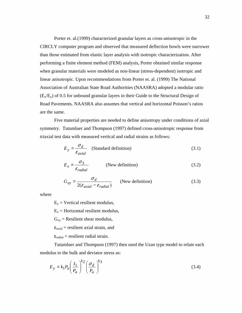
Five material properties are needed to define anisotropy under conditions of axial
symmetry. Tutumluer and Thompson (1997) defined cross-anisotropic response from
triaxial test data with measured vertical and radial strains as follows:
axial
dyE
εσ
= (Standard definition) (3.1)
radialxE
εσ 3= (New definition) (3.2)
)(2 radialaxial
dxyG
εεσ−
= (New definition) (3.3)
where
Ey = Vertical resilient modulus,
Ex = Horizontal resilient modulus,
Gxy = Resilient shear modulus,
εaxial = resilient axial strain, and
εradial = resilient radial strain.
Tutumluer and Thompson (1997) then used the Uzan type model to relate each
modulus to the bulk and deviator stress as:
321
1
k
a
dk
aay PP
IPkE
=
σ (3.4)
33
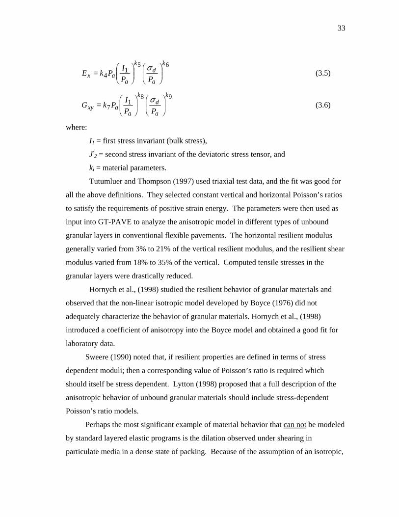
651
4
k
a
dk
aax PP
IPkE
=
σ (3.5)
981
7
k
a
dk
aaxy PP
IPkG
=
σ (3.6)
where:
I1 = first stress invariant (bulk stress),
J/2 = second stress invariant of the deviatoric stress tensor, and
ki = material parameters.
Tutumluer and Thompson (1997) used triaxial test data, and the fit was good for
all the above definitions. They selected constant vertical and horizontal Poisson’s ratios
to satisfy the requirements of positive strain energy. The parameters were then used as
input into GT-PAVE to analyze the anisotropic model in different types of unbound
granular layers in conventional flexible pavements. The horizontal resilient modulus
generally varied from 3% to 21% of the vertical resilient modulus, and the resilient shear
modulus varied from 18% to 35% of the vertical. Computed tensile stresses in the
granular layers were drastically reduced.
Hornych et al., (1998) studied the resilient behavior of granular materials and
observed that the non-linear isotropic model developed by Boyce (1976) did not
adequately characterize the behavior of granular materials. Hornych et al., (1998)
introduced a coefficient of anisotropy into the Boyce model and obtained a good fit for
laboratory data.
Sweere (1990) noted that, if resilient properties are defined in terms of stress
dependent moduli; then a corresponding value of Poisson’s ratio is required which
should itself be stress dependent. Lytton (1998) proposed that a full description of the
anisotropic behavior of unbound granular materials should include stress-dependent
Poisson’s ratio models.
Perhaps the most significant example of material behavior that can not be modeled
by standard layered elastic programs is the dilation observed under shearing in
particulate media in a dense state of packing. Because of the assumption of an isotropic,
34
homogeneous material, traditional layered elastic programs can only accommodate
materials with Poisson’s ratio below 0.5. For most granular materials, a fixed Poisson’s
ratio is normally used. A typical value of Poisson’s ratio lies within the range 0.30 to
0.40. However, when a material dilates, Poisson’s ratios can be as high as 1.20 or higher
(Crockford et al., 1990; Uzan et al, 1992; Allen, 1973). This tendency to dilate is caused
by the motion of particles that tend to roll over one another when a shearing stress is
applied. Most researchers agree that dense graded granular materials start to dilate when
the principal stress ratio exceeds a certain value. Allen (1973) expressed the relationship
between Poisson’s ratio and stress state. Chen and Saleeb (1982), Lade and Nelson
(1987) derived relationships between the Poisson’s ratio and the resilient modulus based
on thermodynamic constraints.
Although there is strong evidence in the literature that nonlinear cross-
anisotropic elastic models are superior to isotropic models in characterizing granular
materials, it has been extremely difficult to determine the cross-anisotropic material
properties of unbound granular materials using the conventional triaxial setup. To obtain
the cross-anisotropic parameters of granular materials, a truly triaxial setup with multi-
axial devices must be used instead of the conventional cylindrical triaxial setup. The
truly triaxial device permits application of three independent principal stresses on six
faces of a cubical specimen of a material.
Graham et al., (1983) proposed a mathematical technique using elasticity theory
to determine anisotropic material parameters from triaxial test data. The technique
proposed by Graham et al., (1983) is not suitable for unbound granular materials because
the material is assumed to be linearly elastic.
Tutumluer et al., (2000) modified the standard AASHTO 294-94 to determine
cross-anisotropic parameters of several granular materials. In the modified test,
Tutumluer et al., (2000) used both triaxial compression and extension tests. The stress
states recommended in AASHTO 294-94 is maintained but the principal stresses are
interchanged after each triaxial compression, to induce a triaxial extension. This way,
35
there is enough data to determine the vertical and horizontal moduli. However, the
resilient shear modulus cannot be determined from the modified AASHTO 294-94 test.
One the objective of this study is to develop an improved testing protocol based
on traditional elasticity theories. The developments of anisotropic resilient model and
testing method for unbound granular materials are discussed in the following sections.
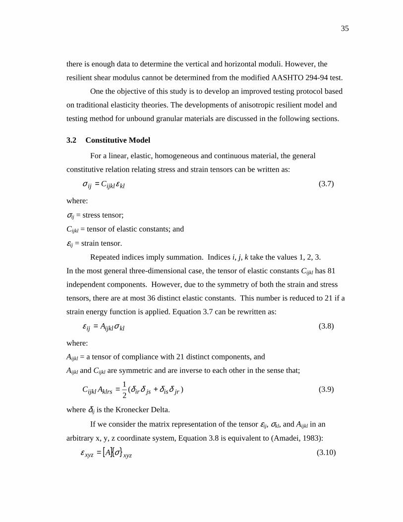
3.2 Constitutive Model
For a linear, elastic, homogeneous and continuous material, the general
constitutive relation relating stress and strain tensors can be written as:
klijklij C εσ = (3.7)
where:
σij = stress tensor;
Cijkl = tensor of elastic constants; and
εij = strain tensor.
Repeated indices imply summation. Indices i, j, k take the values 1, 2, 3.
In the most general three-dimensional case, the tensor of elastic constants Cijkl has 81
independent components. However, due to the symmetry of both the strain and stress
tensors, there are at most 36 distinct elastic constants. This number is reduced to 21 if a
strain energy function is applied. Equation 3.7 can be rewritten as:
klijklij A σε = (3.8)
where:
Aijkl = a tensor of compliance with 21 distinct components, and
Aijkl and Cijkl are symmetric and are inverse to each other in the sense that;
)(21
jrisjsirklrsijkl AC δδδδ += (3.9)
where δij is the Kronecker Delta.
If we consider the matrix representation of the tensor εij, σkl, and Aijkl in an
arbitrary x, y, z coordinate system, Equation 3.8 is equivalent to (Amadei, 1983):
[ ] xyzxyz A σε = (3.10)
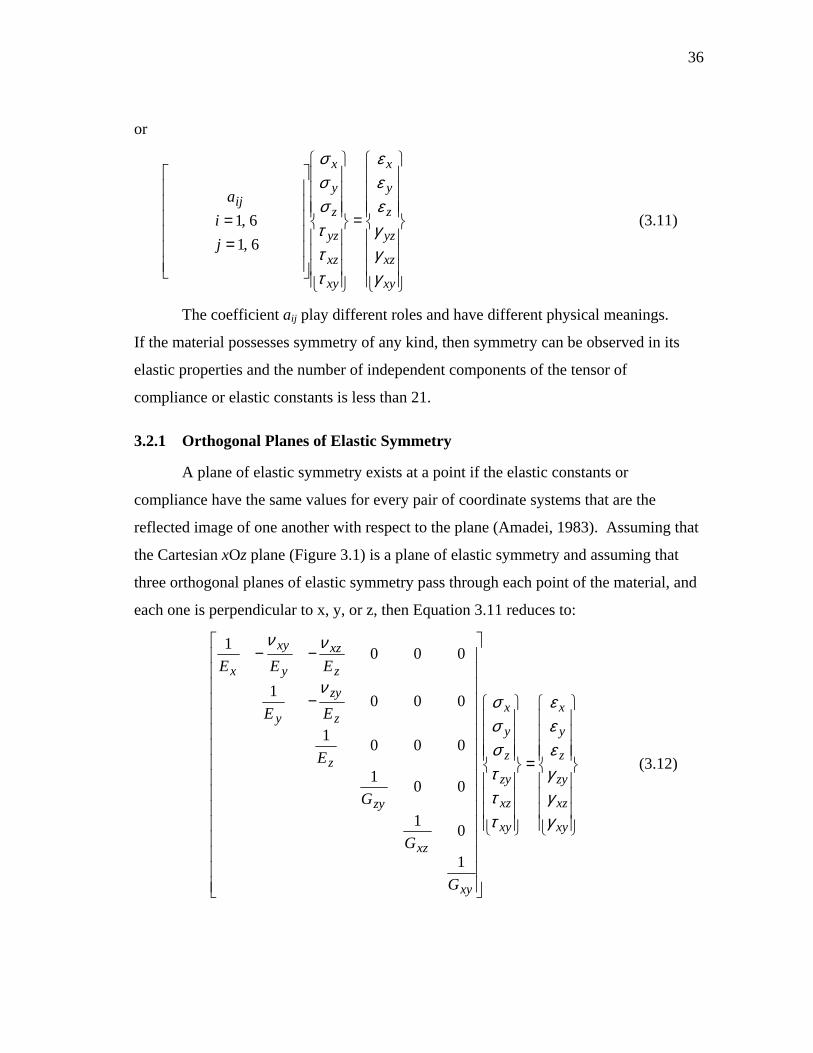
36
or
=
==
xy
xz
yz
z
y
x
xy
xz
yz
z
y
x
ij
ji
a
γγγεεε
τττσσσ
6,16,1 (3.11)
The coefficient aij play different roles and have different physical meanings.
If the material possesses symmetry of any kind, then symmetry can be observed in its
elastic properties and the number of independent components of the tensor of
compliance or elastic constants is less than 21.
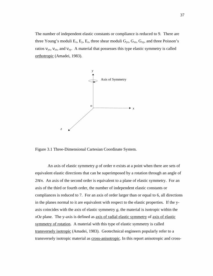
3.2.1 Orthogonal Planes of Elastic Symmetry
A plane of elastic symmetry exists at a point if the elastic constants or
compliance have the same values for every pair of coordinate systems that are the
reflected image of one another with respect to the plane (Amadei, 1983). Assuming that
the Cartesian xOz plane (Figure 3.1) is a plane of elastic symmetry and assuming that
three orthogonal planes of elastic symmetry pass through each point of the material, and
each one is perpendicular to x, y, or z, then Equation 3.11 reduces to:
=
−
−−
xy
xz
zy
z
y
x
xy
xz
zy
z
y
x
xy
xz
zy
z
z
zy
y
z
xz
y
xy
x
G
G
G
E
EE
EEE
γγγεεε
τττσσσ
ν
νν
1
01
001
0001
0001
0001
(3.12)
37
The number of independent elastic constants or compliance is reduced to 9. There are
three Young’s moduli Ex, Ey, Ez, three shear moduli Gyz, Gxz, Gxy, and three Poisson’s
ratios νyx, νzx, and νzy. A material that possesses this type elastic symmetry is called
orthotropic (Amadei, 1983).
x
y
z
o
Axis of Symmetry
Figure 3.1 Three-Dimensional Cartesian Coordinate System.
An axis of elastic symmetry g of order n exists at a point when there are sets of
equivalent elastic directions that can be superimposed by a rotation through an angle of
2π/n. An axis of the second order is equivalent to a plane of elastic symmetry. For an
axis of the third or fourth order, the number of independent elastic constants or
compliances is reduced to 7. For an axis of order larger than or equal to 6, all directions
in the planes normal to it are equivalent with respect to the elastic properties. If the y-
axis coincides with the axis of elastic symmetry g, the material is isotropic within the
xOz plane. The y-axis is defined as axis of radial elastic symmetry of axis of elastic
symmetry of rotation. A material with this type of elastic symmetry is called
transversely isotropic (Amadei, 1983). Geotechnical engineers popularly refer to a
transversely isotropic material as cross-anisotropic. In this report anisotropic and cross-
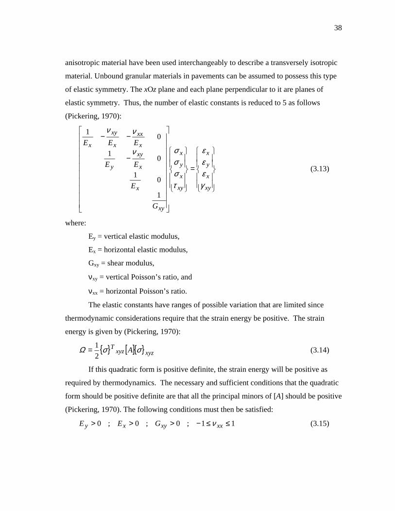
38
anisotropic material have been used interchangeably to describe a transversely isotropic
material. Unbound granular materials in pavements can be assumed to possess this type
of elastic symmetry. The xOz plane and each plane perpendicular to it are planes of
elastic symmetry. Thus, the number of elastic constants is reduced to 5 as follows
(Pickering, 1970):
=
−
−−
xy
x
y
x
xy
x
y
x
xy
x
x
xy
y
x
xx
x
xy
x
G
E
EE
EEE
γεεε
τσσσν
νν
1
01
01
01
(3.13)
where:
Ey = vertical elastic modulus,
Ex = horizontal elastic modulus,
Gxy = shear modulus,
νxy = vertical Poisson’s ratio, and
νxx = horizontal Poisson’s ratio.
The elastic constants have ranges of possible variation that are limited since
thermodynamic considerations require that the strain energy be positive. The strain
energy is given by (Pickering, 1970):
[ ] xyzxyzT A σσΩ
21= (3.14)
If this quadratic form is positive definite, the strain energy will be positive as
required by thermodynamics. The necessary and sufficient conditions that the quadratic
form should be positive definite are that all the principal minors of [A] should be positive
(Pickering, 1970). The following conditions must then be satisfied:
11;0;0;0 ≤≤−>>> xxxyxy GEE ν (3.15)
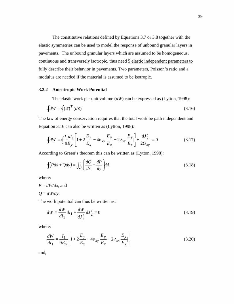
39
The constitutive relations defined by Equations 3.7 or 3.8 together with the
elastic symmetries can be used to model the response of unbound granular layers in
pavements. The unbound granular layers which are assumed to be homogeneous,
continuous and transversely isotropic, thus need 5 elastic independent parameters to
fully describe their behavior in pavements. Two parameters, Poisson’s ratio and a
modulus are needed if the material is assumed to be isotropic.
3.2.2 Anisotropic Work Potential
The elastic work per unit volume (dW) can be expressed as (Lytton, 1998):
∫ ∫= )()( εσ ddW T (3.16)
The law of energy conservation requires that the total work be path independent and
Equation 3.16 can also be written as (Lytton, 1998):
02
24219
/211 =+
−−+=∫ ∫
xyx
yxx
x
yxy
x
y
y GdJ
EE
EE
EE
EdII
dW νν (3.17)
According to Green’s theorem this can be written as (Lytton, 1998):
( )∫ ∫∫
−=+
AdA
dydP
dxdQQdyPdx (3.18)
where:
P = dW/dx, and
Q = dW/dy.
The work potential can thus be written as:
0/2/
21
1=+= dJ
dJdWdI
dIdWdW (3.19)
where:
−−+=
x
yxx
x
yxy
x
y
y EE
EE
EE
EI
dIdW νν 2421
91
1 (3.20)
and,
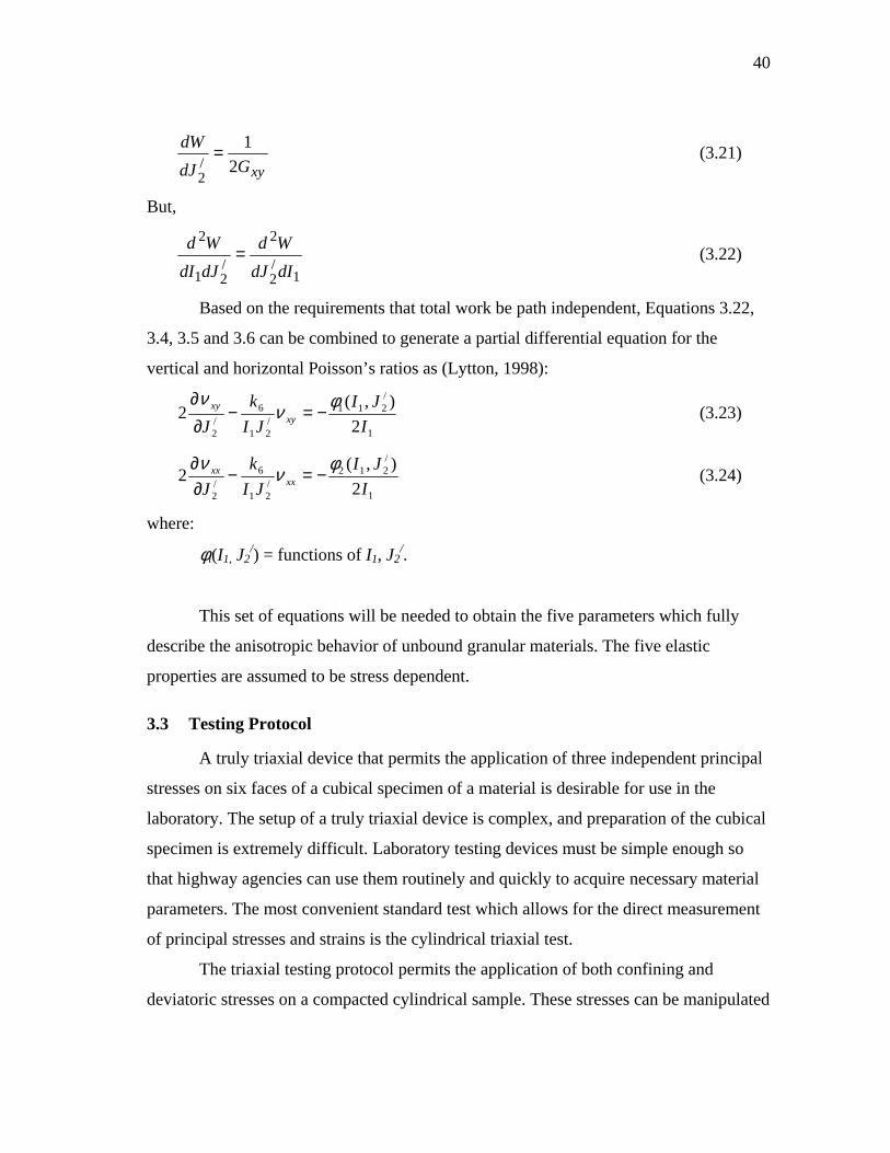
40
xyGdJdW
21
/2
= (3.21)
But,
1/2
2
/21
2
dIdJWd
dJdIWd = (3.22)
Based on the requirements that total work be path independent, Equations 3.22,
3.4, 3.5 and 3.6 can be combined to generate a partial differential equation for the
vertical and horizontal Poisson’s ratios as (Lytton, 1998):
1
/211
/21
6/2 2
),(2I
JIJI
kJ xy
xy φνν
−=−∂∂
(3.23)
1
/212
/21
6/2 2
),(2I
JIJI
kJ xx
xx φνν−=−
∂∂
(3.24)
where:
φi(I1, J2/) = functions of I1, J2
/.
This set of equations will be needed to obtain the five parameters which fully
describe the anisotropic behavior of unbound granular materials. The five elastic
properties are assumed to be stress dependent.
3.3 Testing Protocol
A truly triaxial device that permits the application of three independent principal
stresses on six faces of a cubical specimen of a material is desirable for use in the
laboratory. The setup of a truly triaxial device is complex, and preparation of the cubical
specimen is extremely difficult. Laboratory testing devices must be simple enough so
that highway agencies can use them routinely and quickly to acquire necessary material
parameters. The most convenient standard test which allows for the direct measurement
of principal stresses and strains is the cylindrical triaxial test.
The triaxial testing protocol permits the application of both confining and
deviatoric stresses on a compacted cylindrical sample. These stresses can be manipulated
41
to obtain a variety of stress combinations. The direction of the principal stresses (σ1, σ2,
and σ3) and strains (ε1, ε2, and ε3) are forced to coincide, and this allows for simple
analysis. The particular order of the principal stresses as major, intermediate, and minor
stresses depends on the type of triaxial test performed.
The stress tensor, T in a triaxial test is given by:
=
3
1
2
000000
σσ
σT (3.25)
where:
σ1, σ2 , and σ3 are the principal stresses.
Let directions 1, 2, and 3 be equal to y, x, z in the Cartesian coordinates system,
respectively, then the stress tensor can be expressed as:
=
z
y
xT
σσ
σ
000000
(3.26)
In a conventional triaxial test on compacted cylindrical samples, the intermediate
and minor principal stresses (σ2, and σ3) are the same and the stress tensor becomes:
=
x
y
xT
σσ
σ
000000
(3.27)
This simplification unfortunately reduces the number of equations in Equation
3.13 from 4 to 3. Also, since the shear stress and strain (τxy, and γxy) can not be measured
in a cylindrical triaxial set up, only 2 equations are available to solve for 4 of the 5
material properties of a cross-anisotropic elastic material (Equation 3.28).
=
−−
−−
y
x
x
y
x
x
xy
yx
xyx
xx
x
xy
x
EEE
EEE
ε
ε
σσσ
νν
νν
1
1
(3.28)
42
Equation 3.28 can be written in stress-strain incremental form as:
=
−−
−−
y
x
x
y
x
x
xy
yx
xyx
xx
x
xy
x
EEE
EEE
ε∆
ε∆
σ∆σ∆σ∆
νν
νν
1
1
(3.29)
To numerically solve for the five anisotropic elastic properties, a new testing
protocol was developed. A programmed loading sequence involving ten stress states that
represent typical stresses within unbound granular layers in pavements is used in the
testing protocol. Three different triaxial regimes were established and implemented
within each stress state in the development of the new testing protocol. The following
assumptions were made in developing the testing protocol:
• The elastic moduli obey the Uzan (1988) model,
• The non-linear tangential moduli are smooth functions of the isotropic stress
invariants (Equations 3.4, 3.5, 3.6),
• Variations of these tangential moduli are negligible within infinitesimal changes in
stress at a particular stress state,
• The material is assumed to behave linearly elastic within a small excursion of
stresses.
The three triaxial regimes implemented within each stress state are discussed in
the following sections.
3.3.1 Triaxial Compression Regime
In this test regime, a sample is loaded statically to a target stress state (axial
stress σy, and radial stress, σx). Then radial stress is kept constant while the axial stress is
dynamically cycled in stress increments of ∆σy. Equation 3.29 can then be expressed as:
=
−−
−−
cy
cx
cx
cy
cx
x
xy
yx
xyx
xx
x
xy
x
EEE
EEE
ε∆
ε∆
σ∆σ∆σ∆
νν
νν
1
1
(3.30)
43
where:
∆εxc is a change in radial strain due to an infinitesimal change in axial stress
∆σyc in triaxial compression,
∆εyc is a change in axial strain due to an infinitesimal change in axial stress ∆σy
c
in triaxial compression, and
∆σxc = 0
3.3.2 Triaxial Shear Regime
After a sample is loaded to a static stress state (axial stress σy, and radial stress
σx), a small dynamic axial stress increment of ∆σyS is applied to the sample while the
radial stress is reduced by a small change in dynamic stress of ∆σxS such that:
sy
sx σ∆σ∆
21−= (3.31)
and,
=
−−
−−
sy
sx
sx
sy
sx
x
xy
yx
xyx
xx
x
xy
x
EEE
EEE
ε∆
ε∆
σ∆σ∆σ∆
νν
νν
1
1
(3.32)
The change in first stress invariant, ∆I1 is zero:
021221 =−=+= s
ysy
sx
syI σ∆σ∆σ∆σ∆∆ (3.33)
The change in second invariant of the deviatoric stress tensor, ∆J/2 is given by:
)(31/
2sx
sy
sJ σ∆σ∆∆ −= (3.34)
Substituting Equation 3.31 into 3.34,
2/2 )(
43 s
ysJ σ∆∆ = (3.35)
44
The change in strain energy, ∆ES is given by:
)(21 s
xsx
sy
sy
sx
sx
sE ε∆σ∆ε∆σ∆ε∆σ∆∆ ++= (3.36)
Substituting Equation 3.31 into 3.36 yields,
)(21 s
xsy
sy
sE ε∆ε∆σ∆∆ += (3.37)
But from Equation 3.17 and since the change in first stress invariant, ∆I1, is zero, the
change in strain energy can be written as:
xy
sGJ
E2
/2∆
∆ = (3.38)
Substituting Equations 3.35 and 3.37 into 3.38 yields,
)(43
sx
sy
sy
xyGε∆ε∆
σ∆
−= (3.39)
Thus the triaxial shear regime can be used to determine the shear modulus, Gxy at any
stress state by Equation 3.39.
3.3.3 Triaxial Extension Regime
In this triaxial regime, the static axial stress, σy is reduced by a small change in
dynamic stress, ∆σye while the radial stress, ∆σx is increased by a small dynamic stress
of ∆σxe . Thus, the net change in stress state is in an extension mode but the principal
stresses are not reversed. Here, Equation 3.29 is expressed as:
=
−−
−−
ey
ex
ex
ey
ex
x
xy
yx
xyx
xx
x
xy
x
EEE
EEE
ε∆
ε∆
σ∆σ∆σ∆
νν
νν
1
1
(3.40)
where:
∆εxe is a change in radial strain due to an infinitesimal change in axial stress ∆σy
c
and radial stress ∆σxe, and

45
∆εyc is a change in axial strain due to an infinitesimal change in axial stress ∆σy
c
and radial stress ∆σxe.
The stresses applied and the strains obtained from the three stress regimes
described are used in a system identification scheme to determine the five cross-
anisotropic parameters.
3.4 System Identification Method
The objective of the system identification (SID) process is to estimate the system
characteristics using only input and output data from the system to be identified (Wang
and Lytton, 1993). The simplest method for representing the behavior of a physical
process is to model it with a mathematical representation, for example Equation 3.29.
The model is said to be ‘identified’ when the error between the model and the real
process is minimized to some level. Otherwise the model must be modified until the
desired level of agreement is achieved.
Figure 3.2 is a schematic diagram of the SID procedure. The model response, Yk,
is compared to the actual response of the system, Y, and the error, e, between the two is
used to adjust the parameters of the model by means of an algorithm, which optimizes
some prescribed criterion.
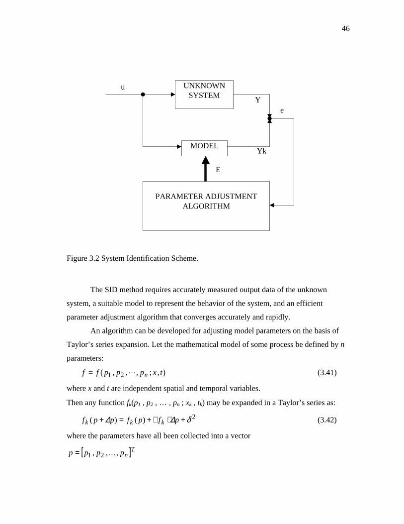
46
UNKNOWNSYSTEM
MODEL
PARAMETER ADJUSTMENTALGORITHM
E
e
uY
Yk
Figure 3.2 System Identification Scheme.
The SID method requires accurately measured output data of the unknown
system, a suitable model to represent the behavior of the system, and an efficient
parameter adjustment algorithm that converges accurately and rapidly.
An algorithm can be developed for adjusting model parameters on the basis of
Taylor’s series expansion. Let the mathematical model of some process be defined by n
parameters:
),;,,,( 21 txpppff nL= (3.41)
where x and t are independent spatial and temporal variables.
Then any function fk(p1 , p2 , … , pn ; xk , tk) may be expanded in a Taylor’s series as:
2)()( δ∆∆ +⋅∇+=+ pfpfppf kkk (3.42)
where the parameters have all been collected into a vector
[ ]Tnpppp ,,, 21 K=
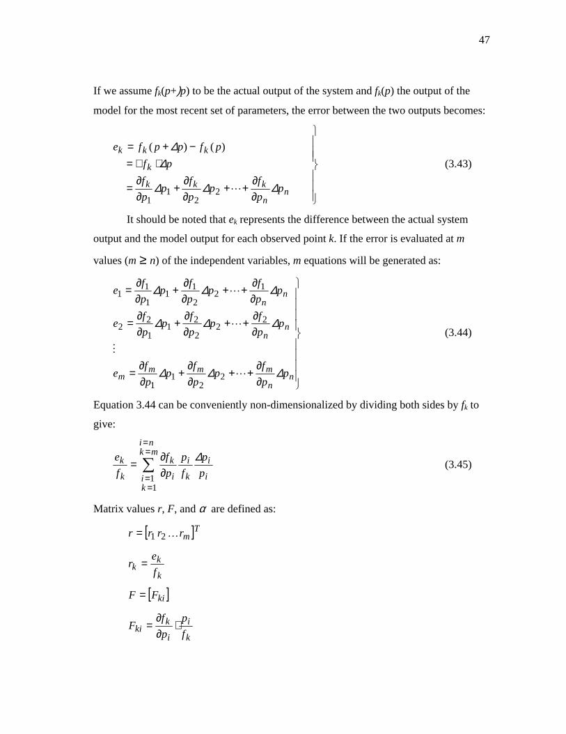
47
If we assume fk(p+)p) to be the actual output of the system and fk(p) the output of the
model for the most recent set of parameters, the error between the two outputs becomes:
∂∂
++∂∂
+∂∂
=
⋅∇=−+=
nn
kkk
k
kkk
ppf
ppf
ppf
pfpfppfe
∆∆∆
∆∆
L22
11
)()( (3.43)
It should be noted that ek represents the difference between the actual system
output and the model output for each observed point k. If the error is evaluated at m
values (m ≥ n) of the independent variables, m equations will be generated as:
∂∂
++∂∂
+∂∂
=
∂∂
++∂∂
+∂∂
=
∂∂
++∂∂
+∂∂
=
nn
mmmm
nn
nn
ppf
ppf
ppf
e
ppfp
pfp
pfe
ppfp
pfp
pfe
∆∆∆
∆∆∆
∆∆∆
L
M
L
L
22
11
22
2
21
1
22
12
2
11
1
11
(3.44)
Equation 3.44 can be conveniently non-dimensionalized by dividing both sides by fk to
give:
∑==
== ∂
∂=
mkni
ki i
i
k
i
i
k
k
kpp
fp
pf
fe
11
∆ (3.45)
Matrix values r, F, and α are defined as:
[ ]Tmrrrr K21=
k
kk f
er =
[ ]kiFF =
k
i
i
kki f
ppf
F ⋅∂∂
=
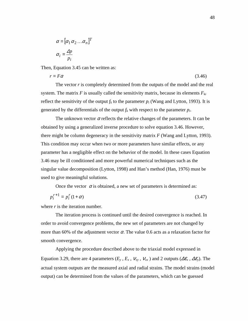
48
[ ]Tnαααα K21=
i
i pp∆α =
Then, Equation 3.45 can be written as:
αFr = (3.46)
The vector r is completely determined from the outputs of the model and the real
system. The matrix F is usually called the sensitivity matrix, because its elements Fki
reflect the sensitivity of the output fk to the parameter pi (Wang and Lytton, 1993). It is
generated by the differentials of the output fk with respect to the parameter pi.
The unknown vector α reflects the relative changes of the parameters. It can be
obtained by using a generalized inverse procedure to solve equation 3.46. However,
there might be column degeneracy in the sensitivity matrix F (Wang and Lytton, 1993).
This condition may occur when two or more parameters have similar effects, or any
parameter has a negligible effect on the behavior of the model. In these cases Equation
3.46 may be ill conditioned and more powerful numerical techniques such as the
singular value decomposition (Lytton, 1998) and Han’s method (Han, 1976) must be
used to give meaningful solutions.
Once the vector α is obtained, a new set of parameters is determined as:
)1(1 α+=+ ri
ri pp (3.47)
where r is the iteration number.
The iteration process is continued until the desired convergence is reached. In
order to avoid convergence problems, the new set of parameters are not changed by
more than 60% of the adjustment vector α. The value 0.6 acts as a relaxation factor for
smooth convergence.
Applying the procedure described above to the triaxial model expressed in
Equation 3.29, there are 4 parameters (Ey , Ex , νxy , νxx ) and 2 outputs (∆εx , ∆εy). The
actual system outputs are the measured axial and radial strains. The model strains (model
output) can be determined from the values of the parameters, which can be guessed
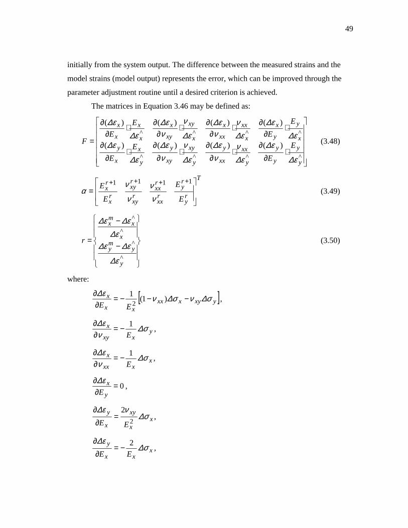
49
initially from the system output. The difference between the measured strains and the
model strains (model output) represents the error, which can be improved through the
parameter adjustment routine until a desired criterion is achieved.
The matrices in Equation 3.46 may be defined as:
⋅∂
∂⋅
∂∂
⋅∂
∂⋅
∂∂
⋅∂
∂⋅
∂∂
⋅∂
∂⋅
∂∂
=
^^^^
^^^^
)()()()(
)()()()(
y
y
y
y
y
xx
xx
y
y
xy
xy
y
y
x
x
yx
y
y
x
x
xx
xx
x
x
xy
xy
x
x
x
x
x
EE
EE
EE
EE
F
ε∆
ε∆
ε∆ν
νε∆
ε∆
ννε∆
ε∆
ε∆ε∆
ε∆ε∆
νν
ε∆ε∆
νν
ε∆ε∆
ε∆
(3.48)
T
ry
ry
rxx
rxx
rxy
rxy
rx
rx
E
E
E
E
=
++++ 1111
νν
ν
να (3.49)
−
−
=
^
^
^
^
y
ymy
x
xmx
r
ε∆
ε∆ε∆ε∆
ε∆ε∆
(3.50)
where:
[ ]yxyxxxxx
x
EEσ∆νσ∆νε∆
−−−=∂∂
)1(12 ,
yxxy
xE
σ∆νε∆ 1−=
∂∂
,
xxxx
xE
σ∆νε∆ 1−=
∂∂
,
0=∂∂
y
xEε∆
,
xx
xy
x
y
EEσ∆
νε∆2
2=
∂∂
,
xxx
y
EEσ∆
ε∆ 2−=∂
∂,
50
0=∂∂
xx
y
νε∆
,
yyy
y
EEσ∆
ε∆2
1−=∂∂
,
∆εxm = measured (actual system) radial strain,
∆εym = measured (actual system) axial strain,
∆εx^ = calculated (model) radial strain, and
∆εy^ = calculated (model) axial strain.
In order to generate enough elements in the sensitivity matrix (F) and to control
row degeneracy, the three stress regimes (triaxial-compression, -shear, and -extension)
were combined to give one F-matrix and one r-matrix at each stress state. Thus, at each
stress state, Equation 3.46 can be rewritten as:
161446 XXX
rrr
FFF
TE
TS
TC
TE
TS
TC
=
α (3.51)
where:
FTC = the sensitivity matrix for triaxial compression regime,
FTS = the sensitivity matrix for triaxial shear regime,
FTE = the sensitivity matrix for triaxial extension regime,
rTC = the r-vector for triaxial compression regime,
rTS = the r-vector for triaxial shear regime, and
rTE = the r-vector for triaxial extension regime.
At a particular stress state, Equation 3.51 is needed by the parameter adjustment
algorithm to determine vertical and horizontal moduli, as well as the vertical and
horizontal Poisson’s ratios. The shear modulus can be determined from Equation 3.39.
51
CHAPTER IV
LABORATORY TESTING
4.1 Equipment
The triaxial test cell was used for testing samples in this study. Triaxial testing
data have been traditionally used to provide input for the material properties in pavement
structural models. The triaxial test has been used with notable success in the field of
geotechnical engineering for applications such as earthquake and tunnel modeling as
well as pavements.
Tests are performed on materials to establish their engineering properties and
these properties are then used in a structural model to determine the stresses and strains
that lead to performance predictions. By setting boundary conditions in the structural
model, it is not necessary for a material property test to exactly mimic the field
condition. However, the testing should, if practical, span a range of expected conditions
so that extrapolations used by the structural model are kept to a minimum.
In the past, the traditional fluid-filled geotechnical type triaxial cell, that enables
confining pressure to be applied to a specimen while a range of vertical loads are
applied, has been the major apparatus used in this type of testing. However, the amount
of time and attention to detail necessary to set up and carry out tests with this equipment
make it unsuitable for production use in the field for Quality-Control/Quality-Assurance
purposes (QC/QA). One other problem associated with the traditional triaxial cell is that
the membrane around the sample is secured to top and bottom platens with rubber bands
(O-rings). This assembly system induces high shear stresses at the top and bottom of
samples tested. To eliminate this problem, it is highly encouraged that sample sizes be
maintained at a 2.0 height to diameter ratio.
In this study, the Rapid Triaxial Testing (RaTT) cell system developed by
Industrial Process Controls (IPC) Melbourne, Australia, was used for testing. The RaTT
cell system is based on a concept that was conceived in Texas Transportation Institute
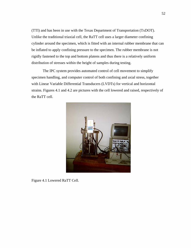
52
(TTI) and has been in use with the Texas Department of Transportation (TxDOT).
Unlike the traditional triaxial cell, the RaTT cell uses a larger diameter confining
cylinder around the specimen, which is fitted with an internal rubber membrane that can
be inflated to apply confining pressure to the specimen. The rubber membrane is not
rigidly fastened to the top and bottom platens and thus there is a relatively uniform
distribution of stresses within the height of samples during testing.
The IPC system provides automated control of cell movement to simplify
specimen handling, and computer control of both confining and axial stress, together
with Linear Variable Differential Transducers (LVDTs) for vertical and horizontal
strains. Figures 4.1 and 4.2 are pictures with the cell lowered and raised, respectively of
the RaTT cell.
Figure 4.1 Lowered RaTT Cell.
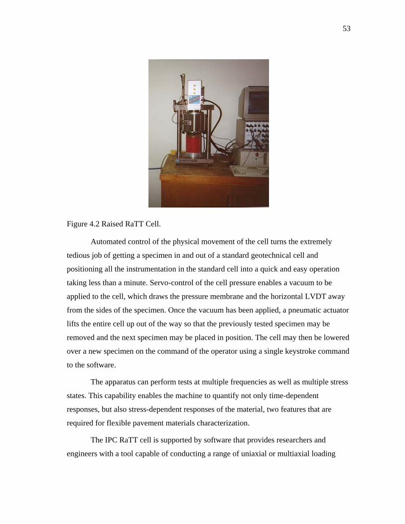
53
Figure 4.2 Raised RaTT Cell.
Automated control of the physical movement of the cell turns the extremely
tedious job of getting a specimen in and out of a standard geotechnical cell and
positioning all the instrumentation in the standard cell into a quick and easy operation
taking less than a minute. Servo-control of the cell pressure enables a vacuum to be
applied to the cell, which draws the pressure membrane and the horizontal LVDT away
from the sides of the specimen. Once the vacuum has been applied, a pneumatic actuator
lifts the entire cell up out of the way so that the previously tested specimen may be
removed and the next specimen may be placed in position. The cell may then be lowered
over a new specimen on the command of the operator using a single keystroke command
to the software.
The apparatus can perform tests at multiple frequencies as well as multiple stress
states. This capability enables the machine to quantify not only time-dependent
responses, but also stress-dependent responses of the material, two features that are
required for flexible pavement materials characterization.
The IPC RaTT cell is supported by software that provides researchers and
engineers with a tool capable of conducting a range of uniaxial or multiaxial loading
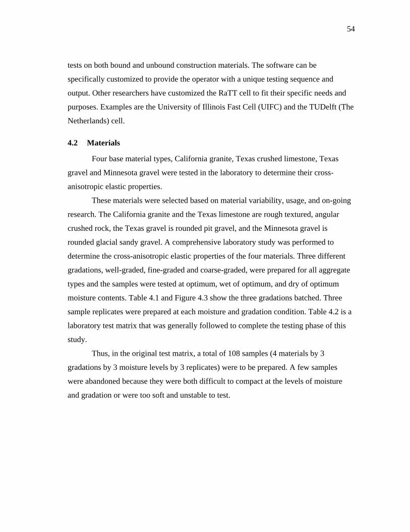
54
tests on both bound and unbound construction materials. The software can be
specifically customized to provide the operator with a unique testing sequence and
output. Other researchers have customized the RaTT cell to fit their specific needs and
purposes. Examples are the University of Illinois Fast Cell (UIFC) and the TUDelft (The
Netherlands) cell.
4.2 Materials
Four base material types, California granite, Texas crushed limestone, Texas
gravel and Minnesota gravel were tested in the laboratory to determine their cross-
anisotropic elastic properties.
These materials were selected based on material variability, usage, and on-going
research. The California granite and the Texas limestone are rough textured, angular
crushed rock, the Texas gravel is rounded pit gravel, and the Minnesota gravel is
rounded glacial sandy gravel. A comprehensive laboratory study was performed to
determine the cross-anisotropic elastic properties of the four materials. Three different
gradations, well-graded, fine-graded and coarse-graded, were prepared for all aggregate
types and the samples were tested at optimum, wet of optimum, and dry of optimum
moisture contents. Table 4.1 and Figure 4.3 show the three gradations batched. Three
sample replicates were prepared at each moisture and gradation condition. Table 4.2 is a
laboratory test matrix that was generally followed to complete the testing phase of this
study.
Thus, in the original test matrix, a total of 108 samples (4 materials by 3
gradations by 3 moisture levels by 3 replicates) were to be prepared. A few samples
were abandoned because they were both difficult to compact at the levels of moisture
and gradation or were too soft and unstable to test.
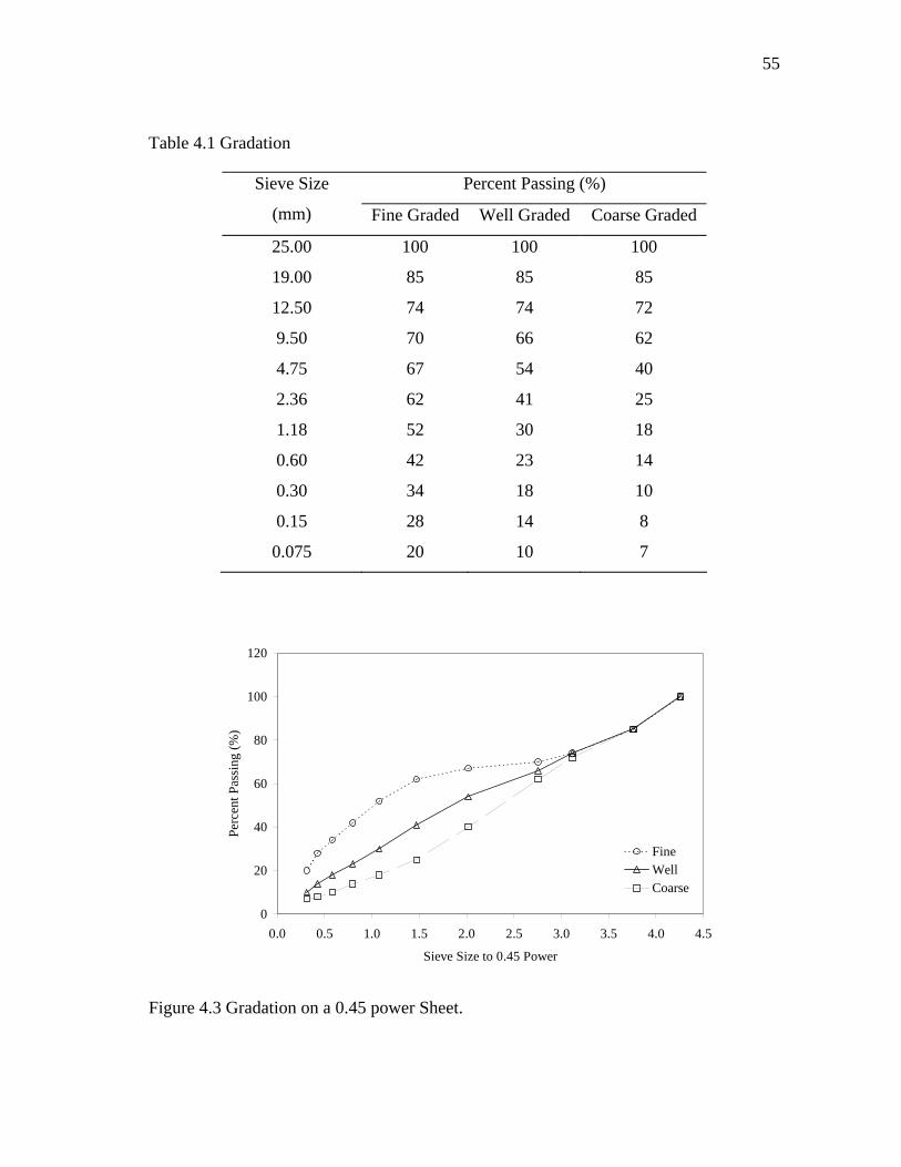
55
Table 4.1 Gradation
Percent Passing (%) Sieve Size
(mm) Fine Graded Well Graded Coarse Graded
25.00 100 100 100
19.00 85 85 85
12.50 74 74 72
9.50 70 66 62
4.75 67 54 40
2.36 62 41 25
1.18 52 30 18
0.60 42 23 14
0.30 34 18 10
0.15 28 14 8
0.075 20 10 7
0
20
40
60
80
100
120
0.0 0.5 1.0 1.5 2.0 2.5 3.0 3.5 4.0 4.5
Sieve Size to 0.45 Power
Perc
ent P
assi
ng (%
)
FineWellCoarse
Figure 4.3 Gradation on a 0.45 power Sheet.
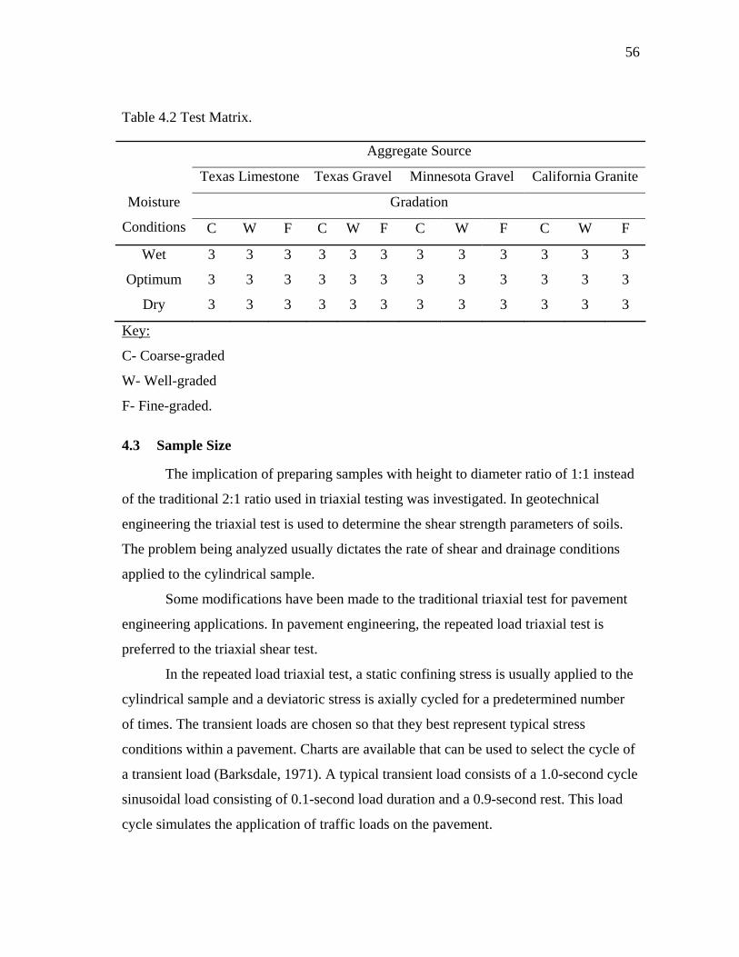
56
Table 4.2 Test Matrix.
Aggregate Source
Texas Limestone Texas Gravel Minnesota Gravel California Granite
Gradation Moisture
Conditions C W F C W F C W F C W F
Wet 3 3 3 3 3 3 3 3 3 3 3 3
Optimum 3 3 3 3 3 3 3 3 3 3 3 3
Dry 3 3 3 3 3 3 3 3 3 3 3 3
Key:
C- Coarse-graded
W- Well-graded
F- Fine-graded.
4.3 Sample Size
The implication of preparing samples with height to diameter ratio of 1:1 instead
of the traditional 2:1 ratio used in triaxial testing was investigated. In geotechnical
engineering the triaxial test is used to determine the shear strength parameters of soils.
The problem being analyzed usually dictates the rate of shear and drainage conditions
applied to the cylindrical sample.
Some modifications have been made to the traditional triaxial test for pavement
engineering applications. In pavement engineering, the repeated load triaxial test is
preferred to the triaxial shear test.
In the repeated load triaxial test, a static confining stress is usually applied to the
cylindrical sample and a deviatoric stress is axially cycled for a predetermined number
of times. The transient loads are chosen so that they best represent typical stress
conditions within a pavement. Charts are available that can be used to select the cycle of
a transient load (Barksdale, 1971). A typical transient load consists of a 1.0-second cycle
sinusoidal load consisting of 0.1-second load duration and a 0.9-second rest. This load
cycle simulates the application of traffic loads on the pavement.
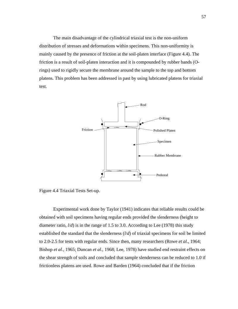
57
The main disadvantage of the cylindrical triaxial test is the non-uniform
distribution of stresses and deformations within specimens. This non-uniformity is
mainly caused by the presence of friction at the soil-platen interface (Figure 4.4). The
friction is a result of soil-platen interaction and it is compounded by rubber bands (O-
rings) used to rigidly secure the membrane around the sample to the top and bottom
platens. This problem has been addressed in past by using lubricated platens for triaxial
test.
Rod
Polished Platen
Specimen
Rubber Membrane
O-Ring
Pedestal
Friction
Figure 4.4 Triaxial Tests Set-up.
Experimental work done by Taylor (1941) indicates that reliable results could be
obtained with soil specimens having regular ends provided the slenderness (height to
diameter ratio, l/d) is in the range of 1.5 to 3.0. According to Lee (1978) this study
established the standard that the slenderness (l/d) of triaxial specimens for soil be limited
to 2.0-2.5 for tests with regular ends. Since then, many researchers (Rowe et al., 1964;
Bishop et al., 1965; Duncan et al., 1968; Lee, 1978) have studied end restraint effects on
the shear strength of soils and concluded that sample slenderness can be reduced to 1.0 if
frictionless platens are used. Rowe and Barden (1964) concluded that if the friction
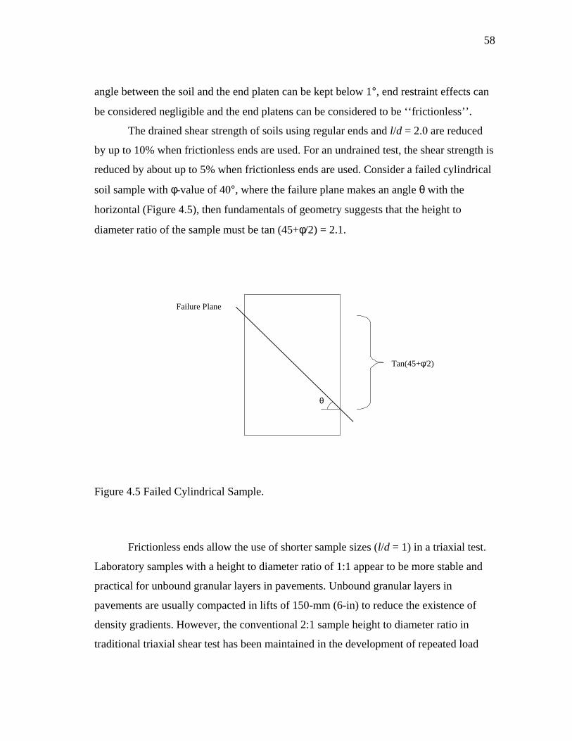
58
angle between the soil and the end platen can be kept below 1°, end restraint effects can
be considered negligible and the end platens can be considered to be ‘‘frictionless’’.
The drained shear strength of soils using regular ends and l/d = 2.0 are reduced
by up to 10% when frictionless ends are used. For an undrained test, the shear strength is
reduced by about up to 5% when frictionless ends are used. Consider a failed cylindrical
soil sample with φ-value of 40°, where the failure plane makes an angle θ with the
horizontal (Figure 4.5), then fundamentals of geometry suggests that the height to
diameter ratio of the sample must be tan (45+φ/2) = 2.1.
Failure Plane
Tan(45+φ/2)
θ
Figure 4.5 Failed Cylindrical Sample.
Frictionless ends allow the use of shorter sample sizes (l/d = 1) in a triaxial test.
Laboratory samples with a height to diameter ratio of 1:1 appear to be more stable and
practical for unbound granular layers in pavements. Unbound granular layers in
pavements are usually compacted in lifts of 150-mm (6-in) to reduce the existence of
density gradients. However, the conventional 2:1 sample height to diameter ratio in
traditional triaxial shear test has been maintained in the development of repeated load
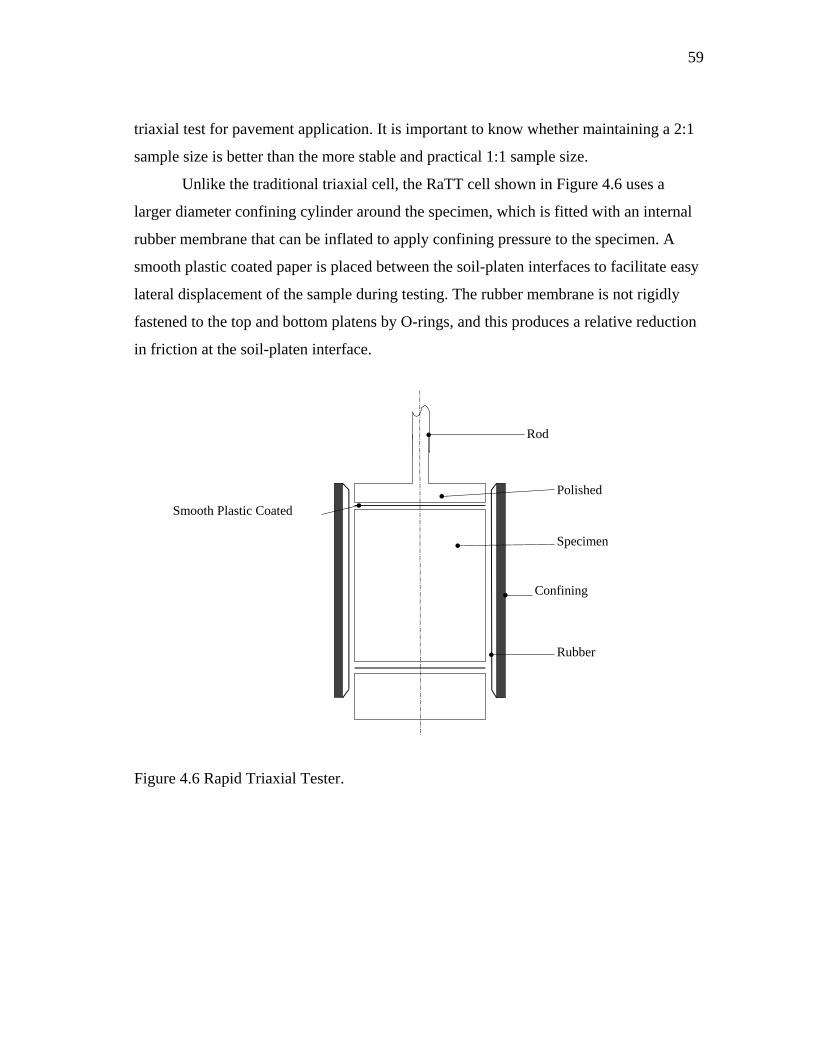
59
triaxial test for pavement application. It is important to know whether maintaining a 2:1
sample size is better than the more stable and practical 1:1 sample size.
Unlike the traditional triaxial cell, the RaTT cell shown in Figure 4.6 uses a
larger diameter confining cylinder around the specimen, which is fitted with an internal
rubber membrane that can be inflated to apply confining pressure to the specimen. A
smooth plastic coated paper is placed between the soil-platen interfaces to facilitate easy
lateral displacement of the sample during testing. The rubber membrane is not rigidly
fastened to the top and bottom platens by O-rings, and this produces a relative reduction
in friction at the soil-platen interface.
Rod
Polished
Specimen
Rubber
Confining
Smooth Plastic Coated
Figure 4.6 Rapid Triaxial Tester.
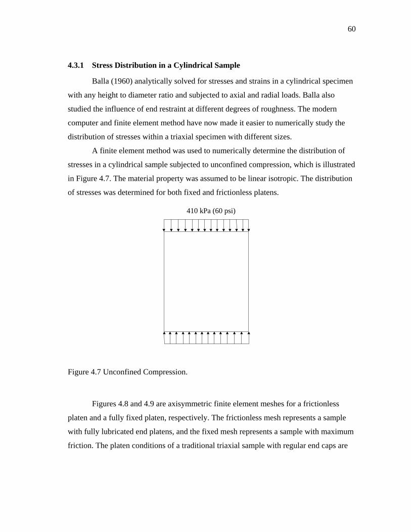
60
4.3.1 Stress Distribution in a Cylindrical Sample
Balla (1960) analytically solved for stresses and strains in a cylindrical specimen
with any height to diameter ratio and subjected to axial and radial loads. Balla also
studied the influence of end restraint at different degrees of roughness. The modern
computer and finite element method have now made it easier to numerically study the
distribution of stresses within a triaxial specimen with different sizes.
A finite element method was used to numerically determine the distribution of
stresses in a cylindrical sample subjected to unconfined compression, which is illustrated
in Figure 4.7. The material property was assumed to be linear isotropic. The distribution
of stresses was determined for both fixed and frictionless platens.
410 kPa (60 psi)
Figure 4.7 Unconfined Compression.
Figures 4.8 and 4.9 are axisymmetric finite element meshes for a frictionless
platen and a fully fixed platen, respectively. The frictionless mesh represents a sample
with fully lubricated end platens, and the fixed mesh represents a sample with maximum
friction. The platen conditions of a traditional triaxial sample with regular end caps are
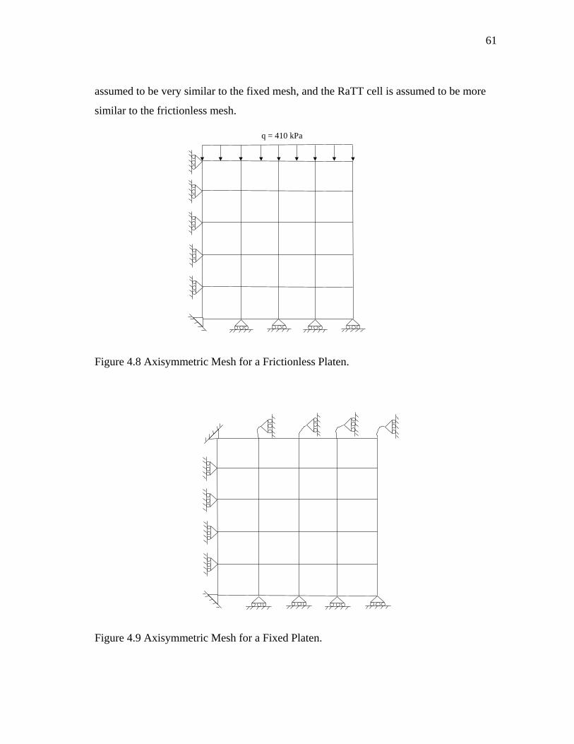
61
assumed to be very similar to the fixed mesh, and the RaTT cell is assumed to be more
similar to the frictionless mesh.
q = 410 kPa
Figure 4.8 Axisymmetric Mesh for a Frictionless Platen.
Figure 4.9 Axisymmetric Mesh for a Fixed Platen.
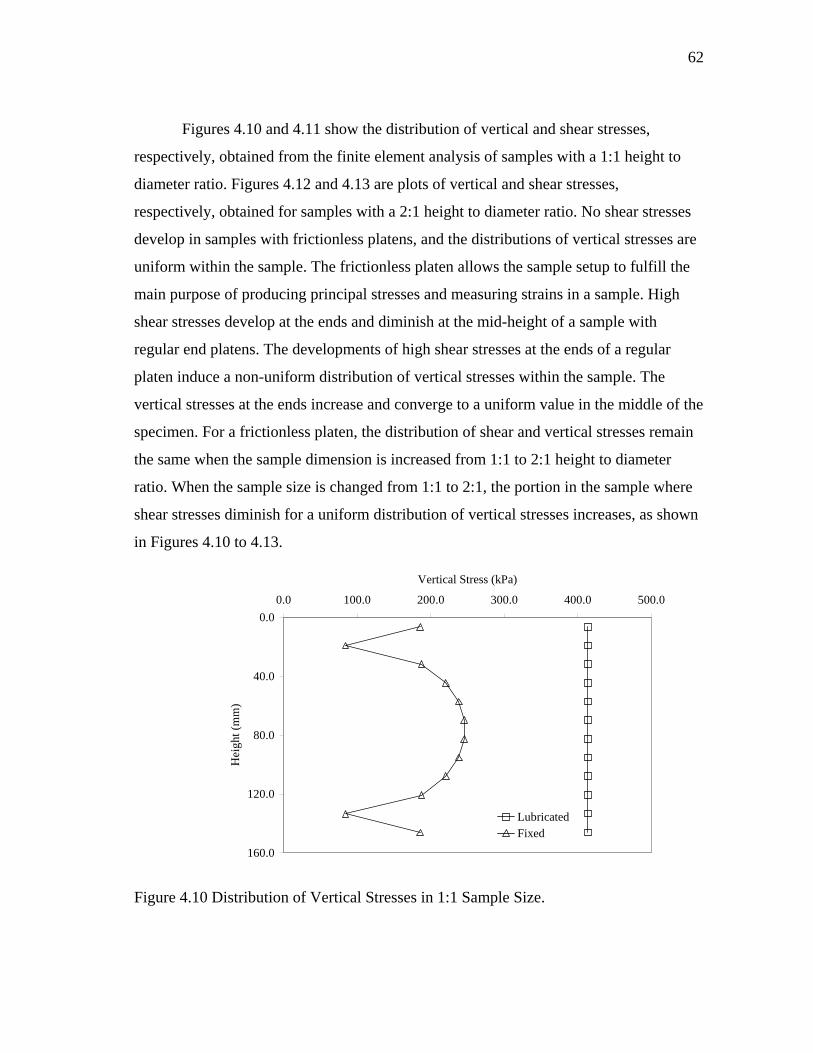
62
Figures 4.10 and 4.11 show the distribution of vertical and shear stresses,
respectively, obtained from the finite element analysis of samples with a 1:1 height to
diameter ratio. Figures 4.12 and 4.13 are plots of vertical and shear stresses,
respectively, obtained for samples with a 2:1 height to diameter ratio. No shear stresses
develop in samples with frictionless platens, and the distributions of vertical stresses are
uniform within the sample. The frictionless platen allows the sample setup to fulfill the
main purpose of producing principal stresses and measuring strains in a sample. High
shear stresses develop at the ends and diminish at the mid-height of a sample with
regular end platens. The developments of high shear stresses at the ends of a regular
platen induce a non-uniform distribution of vertical stresses within the sample. The
vertical stresses at the ends increase and converge to a uniform value in the middle of the
specimen. For a frictionless platen, the distribution of shear and vertical stresses remain
the same when the sample dimension is increased from 1:1 to 2:1 height to diameter
ratio. When the sample size is changed from 1:1 to 2:1, the portion in the sample where
shear stresses diminish for a uniform distribution of vertical stresses increases, as shown
in Figures 4.10 to 4.13.
0.0
40.0
80.0
120.0
160.0
0.0 100.0 200.0 300.0 400.0 500.0
Vertical Stress (kPa)
Hei
ght (
mm
)
LubricatedFixed
Figure 4.10 Distribution of Vertical Stresses in 1:1 Sample Size.
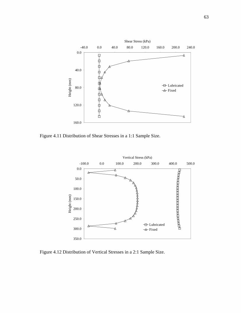
63
0.0
40.0
80.0
120.0
160.0
-40.0 0.0 40.0 80.0 120.0 160.0 200.0 240.0
Shear Stress (kPa)
Hei
ght (
mm
)
LubricatedFixed
Figure 4.11 Distribution of Shear Stresses in a 1:1 Sample Size.
0.0
50.0
100.0
150.0
200.0
250.0
300.0
350.0
-100.0 0.0 100.0 200.0 300.0 400.0 500.0
Vertical Stress (kPa)
Hei
ght (
mm
)
LubricatedFixed
Figure 4.12 Distribution of Vertical Stresses in a 2:1 Sample Size.
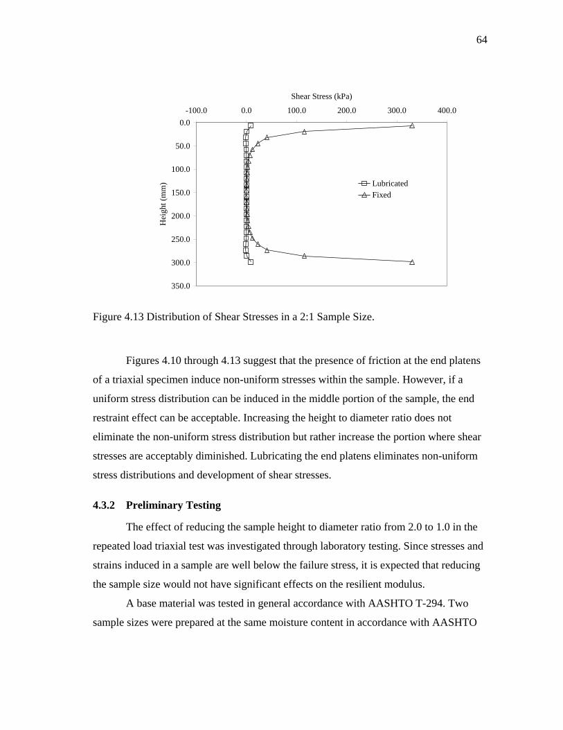
64
0.0
50.0
100.0
150.0
200.0
250.0
300.0
350.0
-100.0 0.0 100.0 200.0 300.0 400.0
Shear Stress (kPa)
Hei
ght (
mm
) LubricatedFixed
Figure 4.13 Distribution of Shear Stresses in a 2:1 Sample Size.
Figures 4.10 through 4.13 suggest that the presence of friction at the end platens
of a triaxial specimen induce non-uniform stresses within the sample. However, if a
uniform stress distribution can be induced in the middle portion of the sample, the end
restraint effect can be acceptable. Increasing the height to diameter ratio does not
eliminate the non-uniform stress distribution but rather increase the portion where shear
stresses are acceptably diminished. Lubricating the end platens eliminates non-uniform
stress distributions and development of shear stresses.
4.3.2 Preliminary Testing
The effect of reducing the sample height to diameter ratio from 2.0 to 1.0 in the
repeated load triaxial test was investigated through laboratory testing. Since stresses and
strains induced in a sample are well below the failure stress, it is expected that reducing
the sample size would not have significant effects on the resilient modulus.
A base material was tested in general accordance with AASHTO T-294. Two
sample sizes were prepared at the same moisture content in accordance with AASHTO
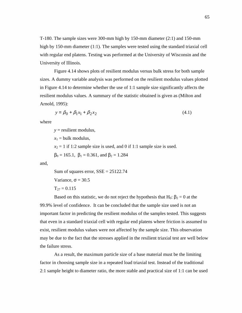
65
T-180. The sample sizes were 300-mm high by 150-mm diameter (2:1) and 150-mm
high by 150-mm diameter (1:1). The samples were tested using the standard triaxial cell
with regular end platens. Testing was performed at the University of Wisconsin and the
University of Illinois.
Figure 4.14 shows plots of resilient modulus versus bulk stress for both sample
sizes. A dummy variable analysis was performed on the resilient modulus values plotted
in Figure 4.14 to determine whether the use of 1:1 sample size significantly affects the
resilient modulus values. A summary of the statistic obtained is given as (Milton and
Arnold, 1995):
22110 xxy βββ ++= (4.1)
where
y = resilient modulus,
x1 = bulk modulus,
x2 = 1 if 1:2 sample size is used, and 0 if 1:1 sample size is used.
β0 = 165.1, β1 = 0.361, and β2 = 1.284
and,
Sum of squares error, SSE = 25122.74
Variance, σ = 30.5
T27 = 0.115
Based on this statistic, we do not reject the hypothesis that H0: β2 = 0 at the
99.9% level of confidence. It can be concluded that the sample size used is not an
important factor in predicting the resilient modulus of the samples tested. This suggests
that even in a standard triaxial cell with regular end platens where friction is assumed to
exist, resilient modulus values were not affected by the sample size. This observation
may be due to the fact that the stresses applied in the resilient triaxial test are well below
the failure stress.
As a result, the maximum particle size of a base material must be the limiting
factor in choosing sample size in a repeated load triaxial test. Instead of the traditional
2:1 sample height to diameter ratio, the more stable and practical size of 1:1 can be used
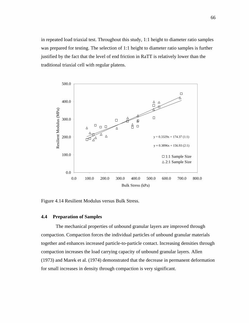
66
in repeated load triaxial test. Throughout this study, 1:1 height to diameter ratio samples
was prepared for testing. The selection of 1:1 height to diameter ratio samples is further
justified by the fact that the level of end friction in RaTT is relatively lower than the
traditional triaxial cell with regular platens.
y = 0.3329x + 174.37 (1:1)
y = 0.3896x + 156.93 (2:1)
0.0
100.0
200.0
300.0
400.0
500.0
0.0 100.0 200.0 300.0 400.0 500.0 600.0 700.0 800.0
Bulk Stress (kPa)
Res
ilien
t Mod
ulus
(MPa
)
1:1 Sample Size2:1 Sample Size
Figure 4.14 Resilient Modulus versus Bulk Stress.
4.4 Preparation of Samples
The mechanical properties of unbound granular layers are improved through
compaction. Compaction forces the individual particles of unbound granular materials
together and enhances increased particle-to-particle contact. Increasing densities through
compaction increases the load carrying capacity of unbound granular layers. Allen
(1973) and Marek et al. (1974) demonstrated that the decrease in permanent deformation
for small increases in density through compaction is very significant.
67
The laboratory compaction characteristics of unbound granular materials are
important to the behavior and performance of a flexible pavement. Three different
compaction methods; impact, vibratory and gyratory shear were investigated in this
study to determine their effects on the anisotropic properties of unbound granular
materials. For each compaction method, two different compactive efforts were
investigated.
4.4.1 Compaction Methods
There are five major compaction methods that are commonly used to fabricate
unbound aggregate specimens for laboratory testing. These methods are briefly
described below (Milberger et. al., 1966).
4.4.1.1 Impact Compaction
The first scientific approach to determine laboratory compaction characteristics
of soils is credited to R.R Proctor (1933). His procedure was slightly revised and
adopted as a standard by the American Association of State Highway Officials in 1939
(AASHTO Designation: T-99). It was later modified to allow higher compaction effort
(AASHTO Designation: T-180). In these methods, the sample is compacted in a rigid
mold by dropping a hammer of known weight from a specified height. One of the main
disadvantages of the impact compaction method is that aggregate orientation and
distribution are dissimilar to that achieved in field compaction. As a result, it is difficult
to achieve reproducible results, and there are some disparities in the stress-strain
distributions predicted in the pavement structure based on the laboratory-derived
resilient moduli. The primary variables that can be controlled in impact compaction are
the weight of the hammer, the height of hammer drop, and the number of blows per
layers. If any of these are increased to achieve high densities at low moisture contents,
much of the additional compactive energy is spent in degrading the material rather than
in compacting it.
68
4.4.1.2 Static Compaction
As the name suggests, samples are compacted in a rigid mold by applying static
compressive stresses to plungers on one or both ends of a specimen. There is no standard
method for applying this method to unbound granular materials. The compaction
characteristics and particle orientation achieved by this method do not reproduce field
compaction. Also, friction between the particles and the mold walls tend to produce
significant density gradients within the sample (Milberger et. al., 1966).
4.4.1.3 Kneading Compaction
Conventional field compaction equipment such as the sheepsfoot and rubber-
tired rollers apply loads with little or no impact, but they produce some kneading action.
According to Milberger et. al. (1966) the California Highway Department developed a
mechanical kneading laboratory compactor in 1937. A revised design of this compactor
was adopted in a standard procedure (AASHO T-173). This method of compaction is not
widely used by highway agencies. Although particle distribution and orientation closely
matches field compaction, some hand finishing is required to prepare samples for testing
in the laboratory (Milberger et. al., 1966).
4.4.1.4 Vibratory Compaction
In this method, the material is confined in a rigid mold, and a surcharge weight is
placed on the surface of the material. Either the wall of the mold is tapped or the entire
mold is placed on a vibrating mechanism. Vibratory compaction has been successfully
applied to the compaction of dry cohesionless soils, primarily sands. The advent of hand
held vibratory equipment has increased the use of vibratory compaction methods for
preparing unbound granular material specimens. Here, layers of material, usually 50-mm
(2-in layers), are compacted to predetermined densities using hand held vibrators in a
rigid mold. Material degradation is reduced using vibratory compaction (Milberger et.
al., 1966).
69
4.4.1.5 Shear Gyratory Compaction
In the early 1940's the Texas Highway Department began compacting specimens
by gyratory shear action (Milberger et. al., 1966). In this method a known stress is
applied to a sample in a rigid mold after the mold has been inclined at an angle. The
mold is rotated at an angle with a stress applied to the sample until the desired density is
achieved. Application of gyratory compaction to asphalt concrete mixtures was one of
the major contributions of the Strategic Highway Research Program (SHRP). This
method is also widely used in Texas to compact unbound granular materials and
bituminous-stabilized bases. The Texas Department of Transportation (TxDOT) has a
standard procedure (Test Method Tex-126-E) for compacting unbound granular and
bituminous base materials with a gyratory compactor. The applied stress and time or
number of gyrations can be varied to achieve a desired density at specific moisture
contents. Researchers at Texas Transportation Institute (Moore and Milberger 1968)
investigated the issue of density gradient, and it was concluded that if the sample height
to diameter ratio is kept below about 1.4, a uniformly compacted specimen is generally
achieved.
Figure 4.15 shows a picture of the gyratory compactor. The development and
validation of the gyratory compactor for use in molding unbound granular materials can
be found in Milberger and Dunlop (1966) and Moore and Milberger (1968). According
to Milberger and Dunlop (1966) the particle distribution and orientation in samples
compacted with the gyratory compaction method closely matches field compaction.
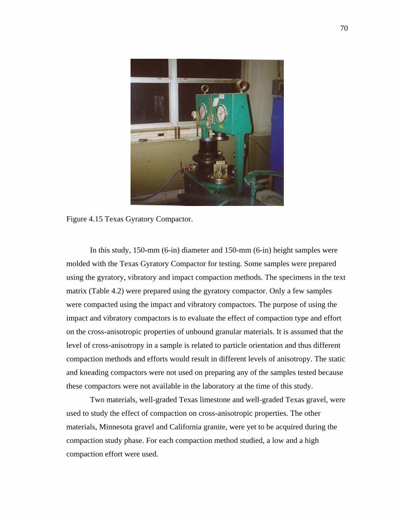
70
Figure 4.15 Texas Gyratory Compactor.
In this study, 150-mm (6-in) diameter and 150-mm (6-in) height samples were
molded with the Texas Gyratory Compactor for testing. Some samples were prepared
using the gyratory, vibratory and impact compaction methods. The specimens in the text
matrix (Table 4.2) were prepared using the gyratory compactor. Only a few samples
were compacted using the impact and vibratory compactors. The purpose of using the
impact and vibratory compactors is to evaluate the effect of compaction type and effort
on the cross-anisotropic properties of unbound granular materials. It is assumed that the
level of cross-anisotropy in a sample is related to particle orientation and thus different
compaction methods and efforts would result in different levels of anisotropy. The static
and kneading compactors were not used on preparing any of the samples tested because
these compactors were not available in the laboratory at the time of this study.
Two materials, well-graded Texas limestone and well-graded Texas gravel, were
used to study the effect of compaction on cross-anisotropic properties. The other
materials, Minnesota gravel and California granite, were yet to be acquired during the
compaction study phase. For each compaction method studied, a low and a high
compaction effort were used.
71
Samples prepared with the impact compaction method were compacted in
general accordance with AASHTO T-180, using a 4.54-kg hammer and a 457-mm drop.
The samples with high compaction effort were prepared by applying either 50 blows per
50-mm thick layers, and the samples with low compaction effort were compacted using
25 blows per 50-mm thick layers.
For the vibratory compaction method, the higher compaction effort samples were
prepared in three lifts (50-mm thick per lift). A hand vibrator was used to compact each
lift until AASHTO T-180 density was achieved. The lower compaction effort samples
were prepared in two lifts (75-mm thick) until 90% of the AASHTO T-180 density was
achieved.
Samples prepared with a high compaction effort using the gyratory compaction
method were fabricated by applying 275-kPa pressure on samples inclined at 3° and
gyrated for 60 seconds. Lower compaction effort samples were prepared by applying
137-kPa pressure on samples inclined at 3° and gyrated for 45 seconds. The gyratory
compactor was set to a constant speed of 30 gyrations per minute. Three lifts of the
specimen were compacted statically and then the entire specimens were compacted
dynamically. After compaction, the top of the samples was leveled with the same
pressure applied during gyrations.
The specimens prepared with the impact and gyratory compaction methods were
tested with the Rapid Triaxial Tester (RaTT) using the testing protocol developed in this
project in which the anisotropic properties of an unbound granular material are
backcalculated using system identification. Details of the testing protocol are discussed
in Section 4.5. The specimens prepared with the vibratory compaction method were
tested with the University of Illinois FastCell (UIFC). The differences between these two
triaxial cells are the mode of application of confining pressure and the range of linear
variable differential transformers (LVDTs). The RaTT uses air for confinement and the
UIFC uses oil. Also, the LVDTs on the UIFC have a wider deflection range and need to
be adjusted for small and large deflections.
72
4.5 Resilient Testing Protocol
The stresses used in the triaxial testing were chosen to represent the stress
conditions induced in a typical base layer of a flexible pavement by traffic loads. The
testing protocol itself involves a programmed loading sequence employing ten static
stress states. At each static stress state, small dynamic changes in stresses are applied to
obtain three triaxial stress regimes such that the net stress changes represent triaxial
compression, triaxial shear, and triaxial extension. The resilient axial and radial strains
are determined for each stress regime and implemented in the system identification
scheme to backcalculate the five anisotropic elastic properties at that particular stress
state.
Before each test is started, the specimen is mounted in the RaTT cell as described
in the operator’s test procedure manuals (IPC, 1998). The loading sequence is outlined in
the following steps:
1. A mounted sample is loaded to a static stress state (axial stress σy, and confining
stress σx, shown as static stress in Table 4.3). The confining stress is then kept
constant while the axial stress is given a small dynamic stress increment of ∆σy,
shown as triaxial compression in Table 4.3. The incremental loading is applied
for 25 repetitions until a stable resilient strain is achieved. A cycle of loading
consists of 1.5 seconds loading followed by 1.5 seconds rest period. Since the
RaTT cell uses air for confinement, the loading cycle was selected to allow for
easy application of variable confinement.
2. At the same static stress state (σx, σy) as in step 1, the axial stress is changed by a
small dynamic stress increment of ∆σy for 25 repetitions as before, while the
radial stress is reduced by ∆σx such that the change in the first stress invariant
(∆I1) is zero in each load cycle. This is shown as triaxial shear in Table 4.3.
3. At the same controlled static stress state (σx, σy) as in step 1, the axial stress is
reduced by a small amount, ∆σy, while the radial stress is increased by ∆σx. Thus,
the net change in stress state is in an extension mode but the principal stresses are
73
not reversed. The dynamic stresses are applied for 25 repetitions as before until
stable resilient strains are achieved. This is shown as triaxial extension in Table
4.3.
4. These steps are repeated for the ten different stress states shown in Table 4.3. At
each stress state, the resilient axial and radial strains are measured for use as
input into the SID scheme.
At the frequencies tested (1.5 seconds loading and 1.5 seconds rest), it takes about
one and a half hours to complete testing on one sample at all ten stress states. The
measured axial and radial strains at each stress state are used as input to the parameter
adjustment routine, Equation 3.51, of the system identification scheme. A computer
program was developed that systematically backcalculates the five anisotropic elastic
material properties based on the SID method.
After each resilient test, part of the sample is tested for soil potential (suction) in
general accordance with ASTM designation D-5298-94. The moisture content of each
sample was determined before and after the resilient test in accordance with ASTM D
2216-92.
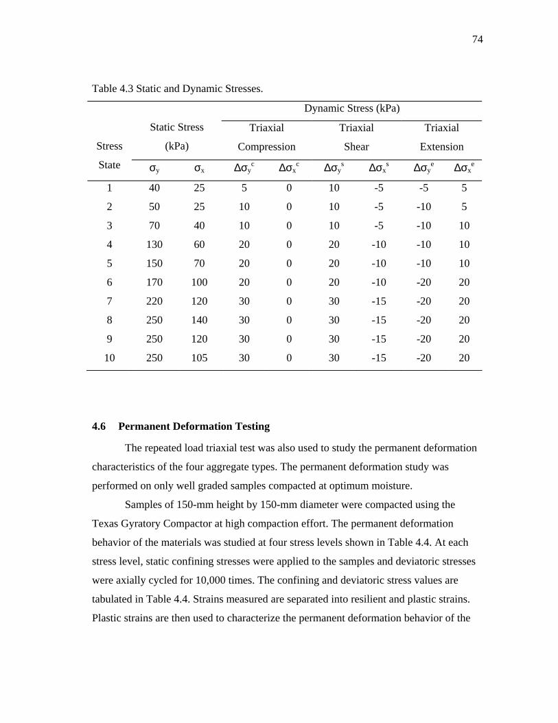
74
Table 4.3 Static and Dynamic Stresses.
Dynamic Stress (kPa)
Static Stress
(kPa)
Triaxial
Compression
Triaxial
Shear
Triaxial
Extension
Stress
State σy σx ∆σyc ∆σx
c ∆σys ∆σx
s ∆σye ∆σx
e
1 40 25 5 0 10 -5 -5 5
2 50 25 10 0 10 -5 -10 5
3 70 40 10 0 10 -5 -10 10
4 130 60 20 0 20 -10 -10 10
5 150 70 20 0 20 -10 -10 10
6 170 100 20 0 20 -10 -20 20
7 220 120 30 0 30 -15 -20 20
8 250 140 30 0 30 -15 -20 20
9 250 120 30 0 30 -15 -20 20
10 250 105 30 0 30 -15 -20 20
4.6 Permanent Deformation Testing
The repeated load triaxial test was also used to study the permanent deformation
characteristics of the four aggregate types. The permanent deformation study was
performed on only well graded samples compacted at optimum moisture.
Samples of 150-mm height by 150-mm diameter were compacted using the
Texas Gyratory Compactor at high compaction effort. The permanent deformation
behavior of the materials was studied at four stress levels shown in Table 4.4. At each
stress level, static confining stresses were applied to the samples and deviatoric stresses
were axially cycled for 10,000 times. The confining and deviatoric stress values are
tabulated in Table 4.4. Strains measured are separated into resilient and plastic strains.
Plastic strains are then used to characterize the permanent deformation behavior of the
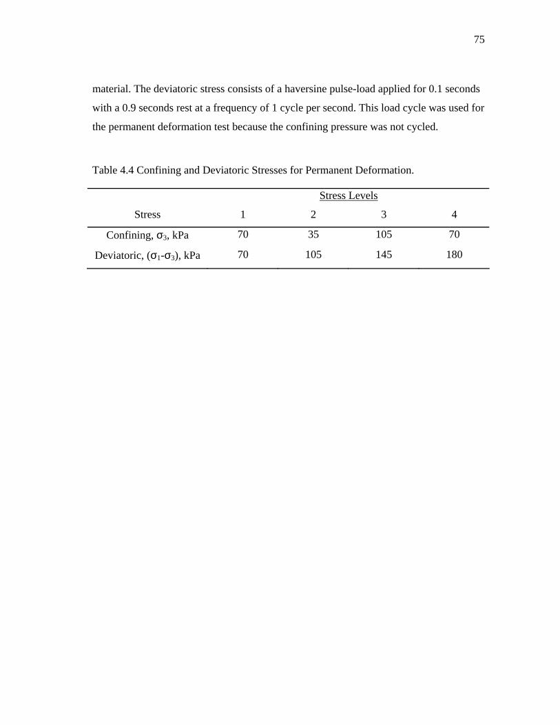
75
material. The deviatoric stress consists of a haversine pulse-load applied for 0.1 seconds
with a 0.9 seconds rest at a frequency of 1 cycle per second. This load cycle was used for
the permanent deformation test because the confining pressure was not cycled.
Table 4.4 Confining and Deviatoric Stresses for Permanent Deformation.
Stress Levels
Stress 1 2 3 4
Confining, σ3, kPa 70 35 105 70
Deviatoric, (σ1-σ3), kPa 70 105 145 180
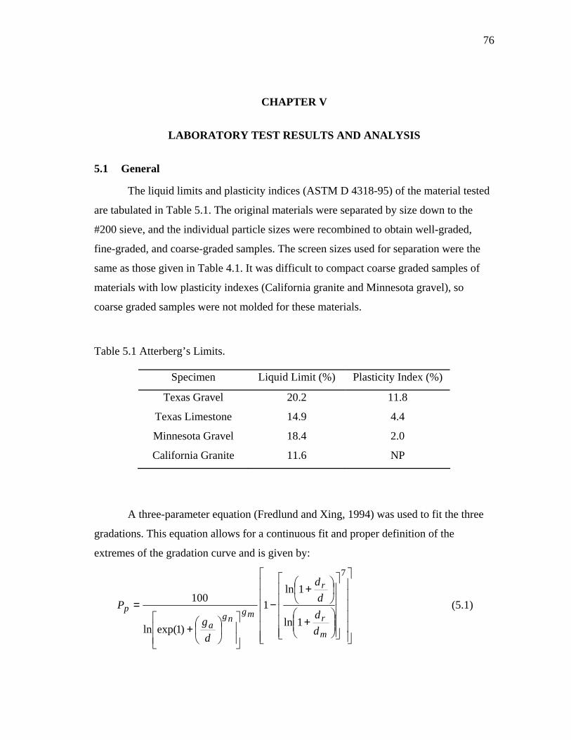
76
CHAPTER V
LABORATORY TEST RESULTS AND ANALYSIS
5.1 General
The liquid limits and plasticity indices (ASTM D 4318-95) of the material tested
are tabulated in Table 5.1. The original materials were separated by size down to the
#200 sieve, and the individual particle sizes were recombined to obtain well-graded,
fine-graded, and coarse-graded samples. The screen sizes used for separation were the
same as those given in Table 4.1. It was difficult to compact coarse graded samples of
materials with low plasticity indexes (California granite and Minnesota gravel), so
coarse graded samples were not molded for these materials.
Table 5.1 Atterberg’s Limits.
Specimen Liquid Limit (%) Plasticity Index (%)
Texas Gravel 20.2 11.8
Texas Limestone 14.9 4.4
Minnesota Gravel 18.4 2.0
California Granite 11.6 NP
A three-parameter equation (Fredlund and Xing, 1994) was used to fit the three
gradations. This equation allows for a continuous fit and proper definition of the
extremes of the gradation curve and is given by:
+
+
−
+
=
7
1ln
1ln1
)1exp(ln
100
m
r
r
mgng
a
p
dddd
dg
P (5.1)
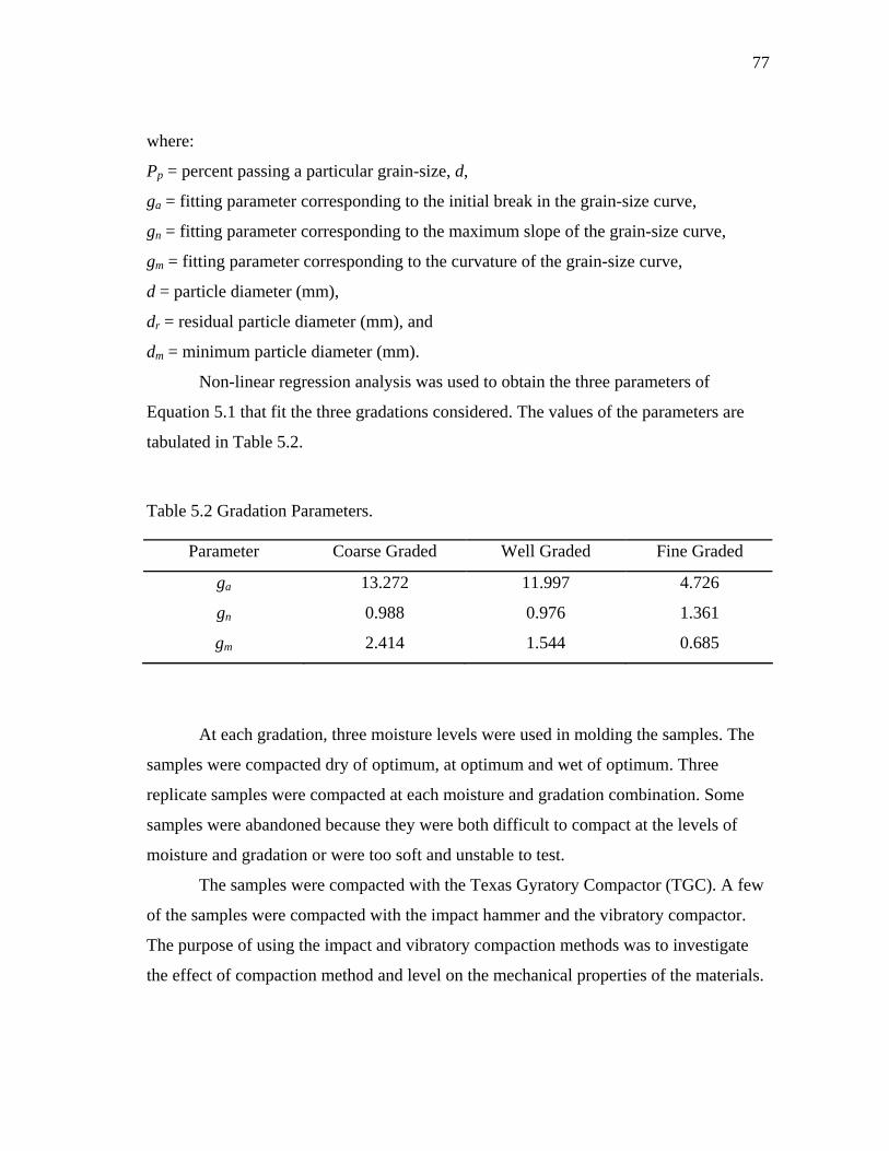
77
where:
Pp = percent passing a particular grain-size, d,
ga = fitting parameter corresponding to the initial break in the grain-size curve,
gn = fitting parameter corresponding to the maximum slope of the grain-size curve,
gm = fitting parameter corresponding to the curvature of the grain-size curve,
d = particle diameter (mm),
dr = residual particle diameter (mm), and
dm = minimum particle diameter (mm).
Non-linear regression analysis was used to obtain the three parameters of
Equation 5.1 that fit the three gradations considered. The values of the parameters are
tabulated in Table 5.2.
Table 5.2 Gradation Parameters.
Parameter Coarse Graded Well Graded Fine Graded
ga 13.272 11.997 4.726
gn 0.988 0.976 1.361
gm 2.414 1.544 0.685
At each gradation, three moisture levels were used in molding the samples. The
samples were compacted dry of optimum, at optimum and wet of optimum. Three
replicate samples were compacted at each moisture and gradation combination. Some
samples were abandoned because they were both difficult to compact at the levels of
moisture and gradation or were too soft and unstable to test.
The samples were compacted with the Texas Gyratory Compactor (TGC). A few
of the samples were compacted with the impact hammer and the vibratory compactor.
The purpose of using the impact and vibratory compaction methods was to investigate
the effect of compaction method and level on the mechanical properties of the materials.
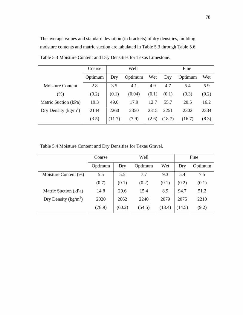
78
The average values and standard deviation (in brackets) of dry densities, molding
moisture contents and matric suction are tabulated in Table 5.3 through Table 5.6.
Table 5.3 Moisture Content and Dry Densities for Texas Limestone.
Coarse Well Fine
Optimum Dry Optimum Wet Dry Optimum Wet
Moisture Content
(%)
2.8
(0.2)
3.5
(0.1)
4.1
(0.04)
4.9
(0.1)
4.7
(0.1)
5.4
(0.3)
5.9
(0.2)
Matric Suction (kPa) 19.3 49.0 17.9 12.7 55.7 20.5 16.2
Dry Density (kg/m3) 2144
(3.5)
2260
(11.7)
2350
(7.9)
2315
(2.6)
2251
(18.7)
2302
(16.7)
2334
(8.3)
Table 5.4 Moisture Content and Dry Densities for Texas Gravel.
Coarse Well Fine
Optimum Dry Optimum Wet Dry Optimum
Moisture Content (%) 5.5
(0.7)
5.5
(0.1)
7.7
(0.2)
9.3
(0.1)
5.4
(0.2)
7.5
(0.1)
Matric Suction (kPa) 14.8 29.6 15.4 8.9 94.7 51.2
Dry Density (kg/m3) 2020
(78.9)
2062
(60.2)
2240
(54.5)
2079
(13.4)
2075
(14.5)
2210
(9.2)
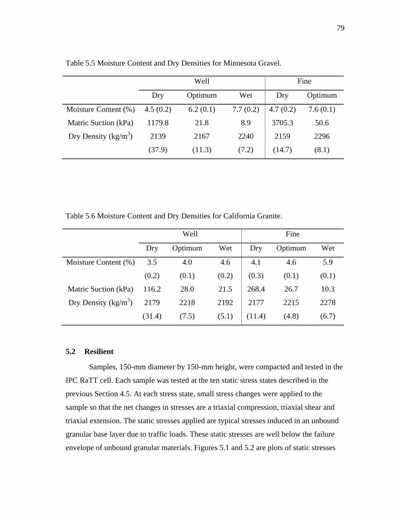
79
Table 5.5 Moisture Content and Dry Densities for Minnesota Gravel.
Well Fine
Dry Optimum Wet Dry Optimum
Moisture Content (%) 4.5 (0.2) 6.2 (0.1) 7.7 (0.2) 4.7 (0.2) 7.6 (0.1)
Matric Suction (kPa) 1179.8 21.8 8.9 3705.3 50.6
Dry Density (kg/m3) 2139
(37.9)
2167
(11.3)
2240
(7.2)
2159
(14.7)
2296
(8.1)
Table 5.6 Moisture Content and Dry Densities for California Granite.
Well Fine
Dry Optimum Wet Dry Optimum Wet
Moisture Content (%) 3.5
(0.2)
4.0
(0.1)
4.6
(0.2)
4.1
(0.3)
4.6
(0.1)
5.9
(0.1)
Matric Suction (kPa) 116.2 28.0 21.5 268.4 26.7 10.3
Dry Density (kg/m3) 2179
(31.4)
2218
(7.5)
2192
(5.1)
2177
(11.4)
2215
(4.8)
2278
(6.7)
5.2 Resilient
Samples, 150-mm diameter by 150-mm height, were compacted and tested in the
IPC RaTT cell. Each sample was tested at the ten static stress states described in the
previous Section 4.5. At each stress state, small stress changes were applied to the
sample so that the net changes in stresses are a triaxial compression, triaxial shear and
triaxial extension. The static stresses applied are typical stresses induced in an unbound
granular base layer due to traffic loads. These static stresses are well below the failure
envelope of unbound granular materials. Figures 5.1 and 5.2 are plots of static stresses
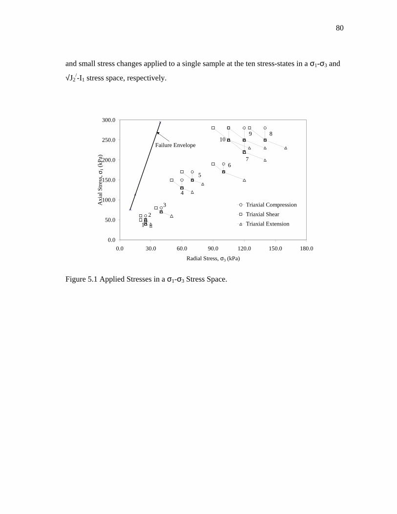
80
and small stress changes applied to a single sample at the ten stress-states in a σ1-σ3 and
√J2/-I1 stress space, respectively.
0.0
50.0
100.0
150.0
200.0
250.0
300.0
0.0 30.0 60.0 90.0 120.0 150.0 180.0
Radial Stress, σ3 (kPa)
Axi
al S
tress
, σ1 (
kPa)
Triaxial CompressionTriaxial ShearTriaxial Extension
9 8
76
5
4
3
2
1
10Failure Envelope
Figure 5.1 Applied Stresses in a σ1-σ3 Stress Space.
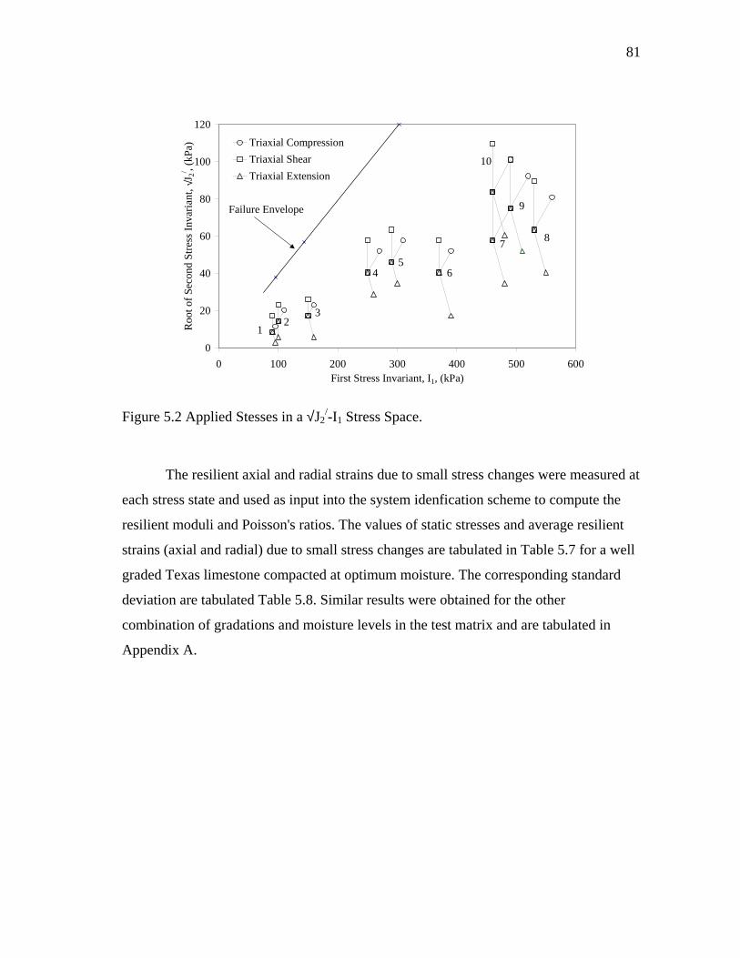
81
0
20
40
60
80
100
120
0 100 200 300 400 500 600First Stress Invariant, I1, (kPa)
Roo
t of S
econ
d St
ress
Inva
riant
, √J 2
/ , (kP
a) Triaxial CompressionTriaxial ShearTriaxial Extension
8
9
10
7
65
4
32
1
Failure Envelope
Figure 5.2 Applied Stesses in a √J2/-I1 Stress Space.
The resilient axial and radial strains due to small stress changes were measured at
each stress state and used as input into the system idenfication scheme to compute the
resilient moduli and Poisson's ratios. The values of static stresses and average resilient
strains (axial and radial) due to small stress changes are tabulated in Table 5.7 for a well
graded Texas limestone compacted at optimum moisture. The corresponding standard
deviation are tabulated Table 5.8. Similar results were obtained for the other
combination of gradations and moisture levels in the test matrix and are tabulated in
Appendix A.
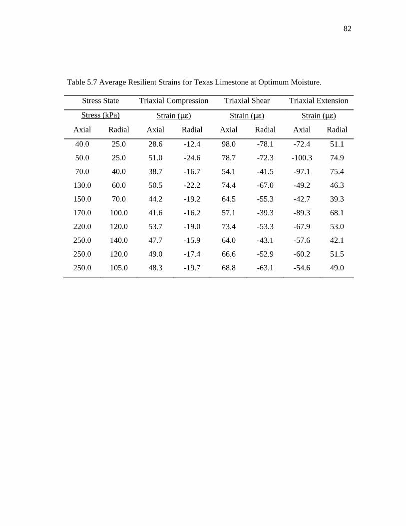
82
Table 5.7 Average Resilient Strains for Texas Limestone at Optimum Moisture.
Stress State Triaxial Compression Triaxial Shear Triaxial Extension
Stress (kPa) Strain (µε) Strain (µε) Strain (µε)
Axial Radial Axial Radial Axial Radial Axial Radial
40.0 25.0 28.6 -12.4 98.0 -78.1 -72.4 51.1
50.0 25.0 51.0 -24.6 78.7 -72.3 -100.3 74.9
70.0 40.0 38.7 -16.7 54.1 -41.5 -97.1 75.4
130.0 60.0 50.5 -22.2 74.4 -67.0 -49.2 46.3
150.0 70.0 44.2 -19.2 64.5 -55.3 -42.7 39.3
170.0 100.0 41.6 -16.2 57.1 -39.3 -89.3 68.1
220.0 120.0 53.7 -19.0 73.4 -53.3 -67.9 53.0
250.0 140.0 47.7 -15.9 64.0 -43.1 -57.6 42.1
250.0 120.0 49.0 -17.4 66.6 -52.9 -60.2 51.5
250.0 105.0 48.3 -19.7 68.8 -63.1 -54.6 49.0

83
Table 5. 8 Standard Deviation of Resilient Strains for Texas Limestone at Optimum
Moisture Content.
Stress State Triaxial Compression Triaxial Shear Triaxial Extension
Stress (kPa) Standard Deviation Standard Deviation Standard Deviation
Axial Radial Axial Radial Axial Radial Axial Radial
40.0 25.0 0.6 0.4 1.0 0.3 1.2 0.4
50.0 25.0 3.0 1.8 6.2 11.1 7.7 9.7
70.0 40.0 1.7 1.3 3.7 4.6 5.5 5.5
130.0 60.0 1.8 1.6 4.7 6.8 4.2 4.2
150.0 70.0 0.7 0.8 4.4 6.3 1.4 3.0
170.0 100.0 2.8 0.6 4.0 2.8 4.7 3.3
220.0 120.0 2.0 2.1 4.7 6.4 6.5 3.8
250.0 140.0 1.9 1.3 3.9 4.6 4.4 3.9
250.0 120.0 1.9 1.0 2.2 4.2 2.5 3.4
250.0 105.0 2.9 2.4 5.4 11.0 3.7 7.2
The measured axial and radial resilient strains are the actual system outputs of
the system identification method. The measured resilient strains act as a nerve center of
the parameter adjustment algorithm of the SID scheme. Therefore, it is very important to
obtain accurate measurements of the resilient strains. In this study, the resilient strains
were measured with externally mounted Linear Variable Differential Transducers
(LVDTs). The LVDTs used are very sensitive to changes in deflection and were suitable
for this study. Two LVDTs each were used to measure axial and radial resilient strains,
respectively and the results are reported as the mean value of these measurements.
A computer program was developed to determine the anisotropic resilient
properties of each sample in the test matrix at the ten stress states using the system
identification method. Figure 5.3 is a schematic of the program structure for the system
identification method. The input parameters include the static and dynamic stresses and
84
the axial and radial resilient strains. Initial values of the five anisotropic resilient
properties are then computed from the dynamic stresses and measured strains. The
computed initial properties are then used to calculate the model output (calculated
strains) from Equations 3.30, 3.32 and 3.40.
The sensitivity matrices F and the r-vectors can then be obtained from Equations
3.48 and 3.50, respectively, for the three triaxial regimes. The three F matrices and three
r-vectors are then combined to obtain one F matrix and one r-vector (Equation 3.51).
The α-vector is then determined from Equation 3.46 and used to compute a new set of
model properties. If the initial values of the five anisotropic properties are precise they
will be equivalent to the new set of model properties and the measured strains, and
calculated strains will also be equivalent to each other. When this occurs, the system is
termed ‘identified’. The criterion for identification is based on the components of the α-
vector. In this study, the criterion is 1%, and this means that the system and model
properties are equivalent whenever the difference between the measured and calculated
strains is less than 1% of the calculated strain. If the 1% criterion is not satisfied, a new
set of model output is calculated and the iteration process is continued until the desired
criterion is reached.
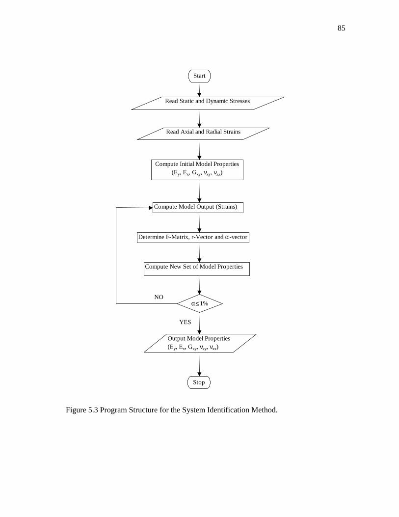
85
Read Static and Dynamic Stresses
Read Axial and Radial Strains
Compute Initial Model Properties(Ey, Ex, Gxy, νxy, νxx)
Compute Model Output (Strains)
Determine F-Matrix, r-Vector and α -vector
α ≤ 1%
Compute New Set of Model Properties
Output Model Properties(Ey, Ex, Gxy, νxy, νxx)
Stop
Start
NO
YES
Figure 5.3 Program Structure for the System Identification Method.
86
As an example, consider the strains obtained at the first stress state for a well-
graded Texas crushed limestone at optimum moisture content (Table 5.7).
Step 1 Input Data
Static Axial Stress, σy = 40.0 kPa
Static Radial Stress, σx = 25.0 kPa
Dynamic Change in Axial Stress for Triaxial Compression, ∆σyc, = 5 kPa
Dynamic Change in Radial Stress for Triaxial Compression, ∆σxc, = 0 kPa
Dynamic Change in Axial Stress for Triaxial Shear, ∆σys, = 10 kPa
Dynamic Change in Radial Stress for Triaxial Shear, ∆σxs, = -5 kPa
Dynamic Change in Axial Stress for Triaxial Extension, ∆σye, = -5 kPa
Dynamic Change in Radial Stress for Triaxial Extension, ∆σxe, = 5 kPa
Axial Resilient Strain for Triaxial Compression, ∆εyc = 28.6E-06
Radial Resilient Strain for Triaxial Compression, ∆εxc = -12.4E-06
Axial Resilient Strain for Triaxial Shear, ∆εys = 98.0E-06
Radial Resilient Strain for Triaxial Shear, ∆εxs = -78.1E-06
Axial Resilient Strain for Triaxial Extension, ∆εye = -72.4E-06
Radial Resilient Strain for Triaxial Extension, ∆εxe = 51.1E-06
Step 2 Initial Model Parameters:
kPaE
E cy
cy
y 17.174825066.28
0.5 =−
==ε∆
σ∆
kPaE
E sx
sx
x 49.64020061.78
0.5 =−−
−==ε∆σ∆
kPaE
G sx
sy
sy
xy 44.4258906)1.780.98(
1043
)(43 =
−+=
−=
ε∆ε∆
σ∆
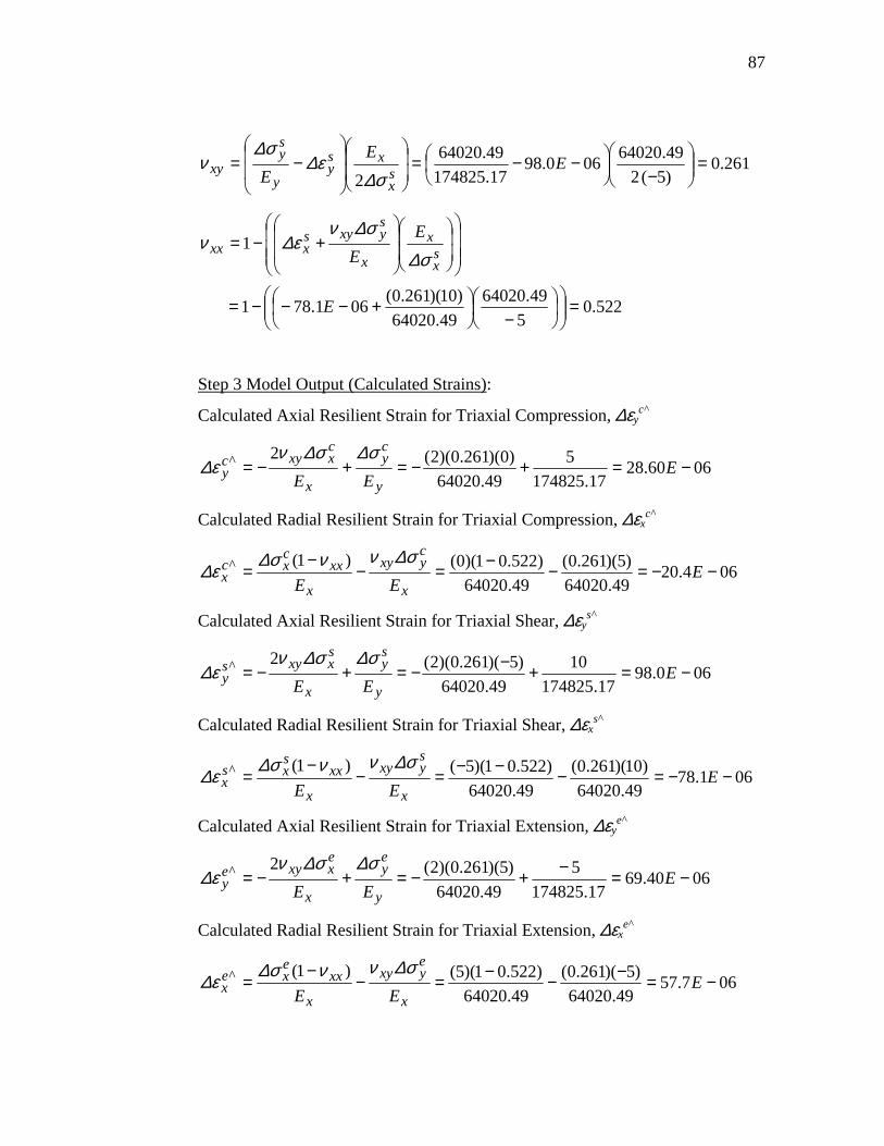
87
261.0)5(249.64020060.98
17.17482549.64020
2=
−
−−=
−= E
EE s
x
xsy
y
sy
xyσ∆
ε∆σ∆
ν
522.05
49.6402049.64020
)10)(261.0(061.781
1
=
−
+−−−=
+−=
E
EE s
x
x
x
syxys
xxxσ∆
σ∆νε∆ν
Step 3 Model Output (Calculated Strains):
Calculated Axial Resilient Strain for Triaxial Compression, ∆εyc^
0660.2817.174825
549.64020
)0)(261.0)(2(2^ −=+−=+−= EEE y
cy
x
cxxyc
yσ∆σ∆ν
ε∆
Calculated Radial Resilient Strain for Triaxial Compression, ∆εxc^
064.2049.64020
)5)(261.0(49.64020
)522.01)(0()1(^ −−=−−=−−
= EEE x
cyxy
x
xxcxc
xσ∆ννσ∆ε∆
Calculated Axial Resilient Strain for Triaxial Shear, ∆εys^
060.9817.174825
1049.64020
)5)(261.0)(2(2^ −=+−−=+−= EEE y
sy
x
sxxys
yσ∆σ∆ν
ε∆
Calculated Radial Resilient Strain for Triaxial Shear, ∆εxs^
061.7849.64020
)10)(261.0(49.64020
)522.01)(5()1(^ −−=−−−=−−
= EEE x
syxy
x
xxsxs
xσ∆ννσ∆ε∆
Calculated Axial Resilient Strain for Triaxial Extension, ∆εye^
0640.6917.174825
549.64020
)5)(261.0)(2(2^ −=−+−=+−= EEE y
ey
x
exxye
yσ∆σ∆ν
ε∆
Calculated Radial Resilient Strain for Triaxial Extension, ∆εxe^
067.5749.64020
)5)(261.0(49.64020
)522.01)(5()1(^ −=−−−=−−
= EEE x
eyxy
x
xxexe
xσ∆ννσ∆ε∆
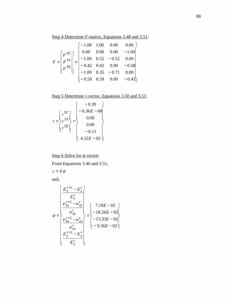
88
Step 4 Determine F-matrix, Equations 3.48 and 3.51:
−−−−
−−−−
−−
=
=
41.000.059.059.000.071.035.000.158.000.042.042.0
00.052.052.000.100.100.000.000.0
00.000.000.100.1
TE
TS
TC
FFF
F
Step 5 Determine r-vector, Equations 3.50 and 3.51:
−−
−−−
=
=
0232.411.0
00.000.0
0836.639.0
E
E
rrr
rTE
TS
TC
Step 6 Solve for α-vector:
From Equations 3.46 and 3.51,
αFr =
and,
−−−−−−
−
=
−
−
−
−
=
+
+
+
+
0236.90233.130226.18
0219.7
1
1
1
1
EEE
E
E
EE
E
EE
ry
ry
ry
rxx
rxx
rxx
rxy
rxy
rxy
rx
rx
rx
ννν
ν
νν
α
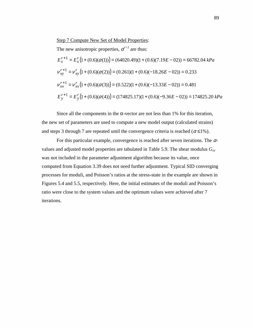
89
Step 7 Compute New Set of Model Properties:
The new anisotropic properties, αr+1 are thus:
( ) kPaEEE rx
rx 04.66782))0219.7)(6.0(1)(49.64020())1()(6.0(11 =−+=+=+ α
( ) 233.0))0226.18)(6.0(1)(261.0())2()(6.0(11 =−−+=+=+ Erxy
rxy ανν
( ) 481.0))0233.13)(6.0(1)(522.0())3()(6.0(11 =−−+=+=+ Erxx
rxx ανν
( ) kPaEEE ry
ry 20.174825))0236.9)(6.0(1)(17.174825())4()(6.0(11 =−−+=+=+ α
Since all the components in the α-vector are not less than 1% for this iteration,
the new set of parameters are used to compute a new model output (calculated strains)
and steps 3 through 7 are repeated until the convergence criteria is reached (α ≤1%).
For this particular example, convergence is reached after seven iterations. The α-
values and adjusted model properties are tabulated in Table 5.9. The shear modulus Gxy
was not included in the parameter adjustment algorithm because its value, once
computed from Equation 3.39 does not need further adjustment. Typical SID converging
processes for moduli, and Poisson’s ratios at the stress-state in the example are shown in
Figures 5.4 and 5.5, respectively. Here, the initial estimates of the moduli and Poisson’s
ratio were close to the system values and the optimum values were achieved after 7
iterations.
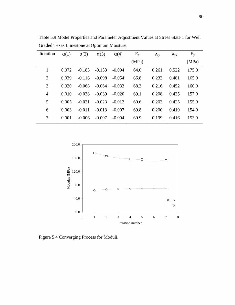
90
Table 5.9 Model Properties and Parameter Adjustment Values at Stress State 1 for Well
Graded Texas Limestone at Optimum Moisture.
Iteration α(1) α(2) α(3) α(4) Ex
(MPa)
νxy νxx Ey
(MPa)
1 0.072 -0.183 -0.133 -0.094 64.0 0.261 0.522 175.0
2 0.039 -0.116 -0.098 -0.054 66.8 0.233 0.481 165.0
3 0.020 -0.068 -0.064 -0.033 68.3 0.216 0.452 160.0
4 0.010 -0.038 -0.039 -0.020 69.1 0.208 0.435 157.0
5 0.005 -0.021 -0.023 -0.012 69.6 0.203 0.425 155.0
6 0.003 -0.011 -0.013 -0.007 69.8 0.200 0.419 154.0
7 0.001 -0.006 -0.007 -0.004 69.9 0.199 0.416 153.0
0.0
40.0
80.0
120.0
160.0
200.0
0 1 2 3 4 5 6 7 8
Iteration number
Mod
ulus
(MPa
)
ExEy
Figure 5.4 Converging Process for Moduli.
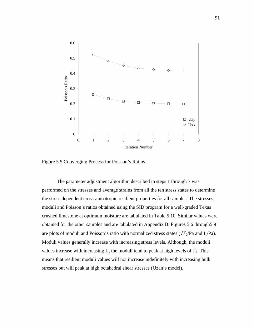
91
0
0.1
0.2
0.3
0.4
0.5
0.6
0 1 2 3 4 5 6 7 8
Iteration Number
Pois
son'
s Rat
io
UxyUxx
Figure 5.5 Converging Process for Poisson’s Ratios.
The parameter adjustment algorithm described in steps 1 through 7 was
performed on the stresses and average strains from all the ten stress states to determine
the stress dependent cross-anisotropic resilient properties for all samples. The stresses,
moduli and Poisson’s ratios obtained using the SID program for a well-graded Texas
crushed limestone at optimum moisture are tabulated in Table 5.10. Similar values were
obtained for the other samples and are tabulated in Appendix B. Figures 5.6 through5.9
are plots of moduli and Poisson’s ratio with normalized stress states (√J/2/Pa and I1/Pa).
Moduli values generally increase with increasing stress levels. Although, the moduli
values increase with increasing I1, the moduli tend to peak at high levels of J/2. This
means that resilient moduli values will not increase indefinitely with increasing bulk
stresses but will peak at high octahedral shear stresses (Uzan’s model).
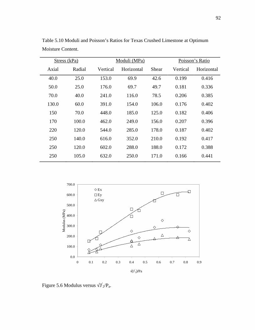
92
Table 5.10 Moduli and Poisson’s Ratios for Texas Crushed Limestone at Optimum
Moisture Content.
Stress (kPa) Moduli (MPa) Poisson’s Ratio
Axial Radial Vertical Horizontal Shear Vertical Horizontal
40.0 25.0 153.0 69.9 42.6 0.199 0.416
50.0 25.0 176.0 69.7 49.7 0.181 0.336
70.0 40.0 241.0 116.0 78.5 0.206 0.385
130.0 60.0 391.0 154.0 106.0 0.176 0.402
150 70.0 448.0 185.0 125.0 0.182 0.406
170 100.0 462.0 249.0 156.0 0.207 0.396
220 120.0 544.0 285.0 178.0 0.187 0.402
250 140.0 616.0 352.0 210.0 0.192 0.417
250 120.0 602.0 288.0 188.0 0.172 0.388
250 105.0 632.0 250.0 171.0 0.166 0.441
0.0
100.0
200.0
300.0
400.0
500.0
600.0
700.0
0 0.1 0.2 0.3 0.4 0.5 0.6 0.7 0.8 0.9
√(J/2)/Pa
Mod
ulus
(MPa
)
ExEyGxy
Figure 5.6 Modulus versus √J/2/Pa.
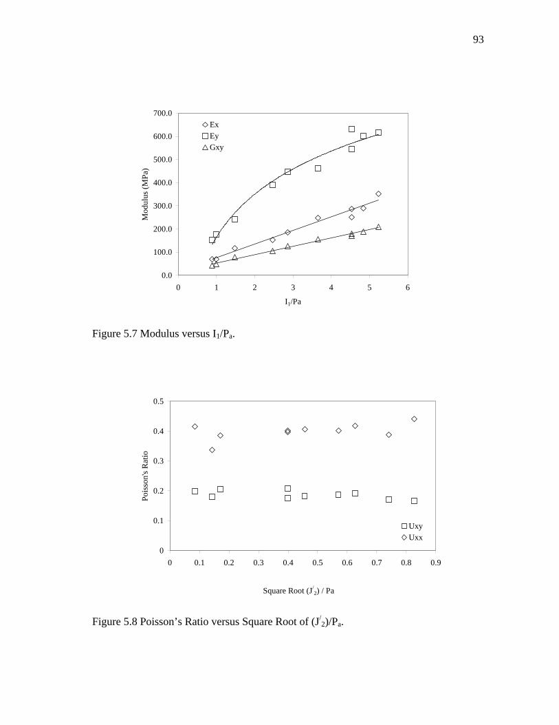
93
0.0
100.0
200.0
300.0
400.0
500.0
600.0
700.0
0 1 2 3 4 5 6
I1/Pa
Mod
ulus
(MPa
)
ExEyGxy
Figure 5.7 Modulus versus I1/Pa.
0
0.1
0.2
0.3
0.4
0.5
0 0.1 0.2 0.3 0.4 0.5 0.6 0.7 0.8 0.9
Square Root (J/2) / Pa
Pois
son'
s Rat
io
UxyUxx
Figure 5.8 Poisson’s Ratio versus Square Root of (J/2)/Pa.
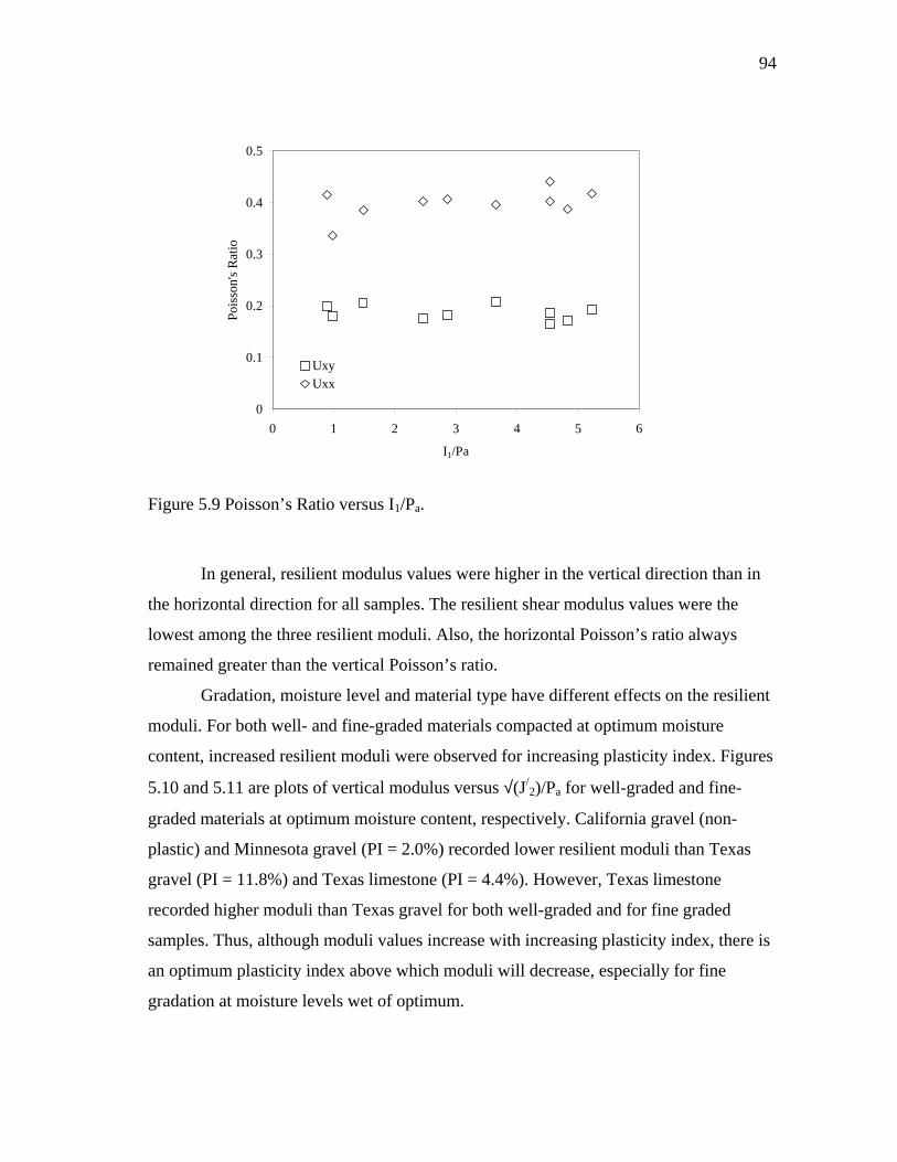
94
0
0.1
0.2
0.3
0.4
0.5
0 1 2 3 4 5 6
I1/Pa
Pois
son'
s Rat
io
UxyUxx
Figure 5.9 Poisson’s Ratio versus I1/Pa.
In general, resilient modulus values were higher in the vertical direction than in
the horizontal direction for all samples. The resilient shear modulus values were the
lowest among the three resilient moduli. Also, the horizontal Poisson’s ratio always
remained greater than the vertical Poisson’s ratio.
Gradation, moisture level and material type have different effects on the resilient
moduli. For both well- and fine-graded materials compacted at optimum moisture
content, increased resilient moduli were observed for increasing plasticity index. Figures
5.10 and 5.11 are plots of vertical modulus versus √(J/2)/Pa for well-graded and fine-
graded materials at optimum moisture content, respectively. California gravel (non-
plastic) and Minnesota gravel (PI = 2.0%) recorded lower resilient moduli than Texas
gravel (PI = 11.8%) and Texas limestone (PI = 4.4%). However, Texas limestone
recorded higher moduli than Texas gravel for both well-graded and for fine graded
samples. Thus, although moduli values increase with increasing plasticity index, there is
an optimum plasticity index above which moduli will decrease, especially for fine
gradation at moisture levels wet of optimum.
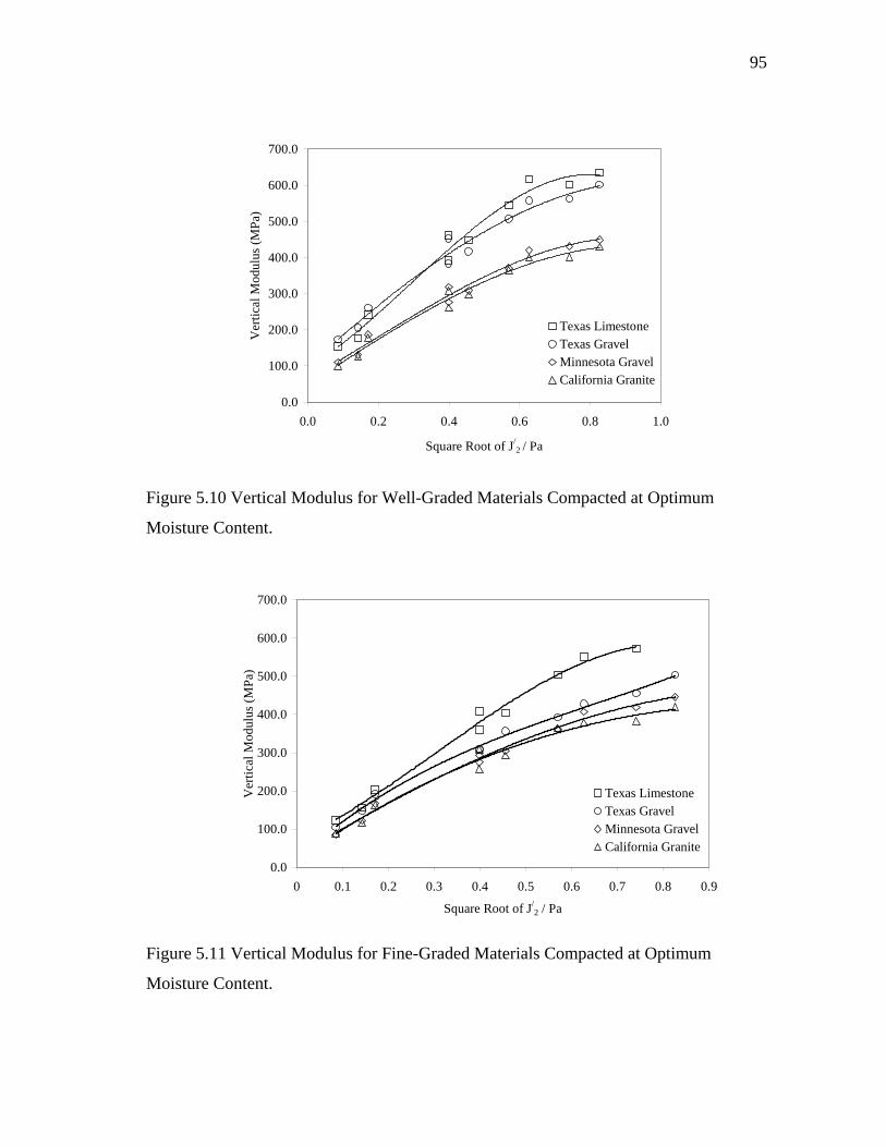
95
0.0
100.0
200.0
300.0
400.0
500.0
600.0
700.0
0.0 0.2 0.4 0.6 0.8 1.0
Square Root of J/2 / Pa
Ver
tical
Mod
ulus
(MPa
)
Texas LimestoneTexas GravelMinnesota GravelCalifornia Granite
Figure 5.10 Vertical Modulus for Well-Graded Materials Compacted at Optimum
Moisture Content.
0.0
100.0
200.0
300.0
400.0
500.0
600.0
700.0
0 0.1 0.2 0.3 0.4 0.5 0.6 0.7 0.8 0.9
Square Root of J/2 / Pa
Ver
tical
Mod
ulus
(MPa
)
Texas LimestoneTexas GravelMinnesota GravelCalifornia Granite
Figure 5.11 Vertical Modulus for Fine-Graded Materials Compacted at Optimum
Moisture Content.
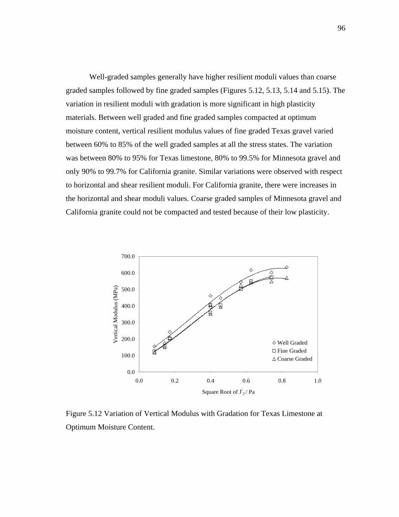
96
Well-graded samples generally have higher resilient moduli values than coarse
graded samples followed by fine graded samples (Figures 5.12, 5.13, 5.14 and 5.15). The
variation in resilient moduli with gradation is more significant in high plasticity
materials. Between well graded and fine graded samples compacted at optimum
moisture content, vertical resilient modulus values of fine graded Texas gravel varied
between 60% to 85% of the well graded samples at all the stress states. The variation
was between 80% to 95% for Texas limestone, 80% to 99.5% for Minnesota gravel and
only 90% to 99.7% for California granite. Similar variations were observed with respect
to horizontal and shear resilient moduli. For California granite, there were increases in
the horizontal and shear moduli values. Coarse graded samples of Minnesota gravel and
California granite could not be compacted and tested because of their low plasticity.
0.0
100.0
200.0
300.0
400.0
500.0
600.0
700.0
0.0 0.2 0.4 0.6 0.8 1.0
Square Root of J/2 / Pa
Ver
tical
Mod
ulus
(MPa
)
Well GradedFine GradedCoarse Graded
Figure 5.12 Variation of Vertical Modulus with Gradation for Texas Limestone at
Optimum Moisture Content.
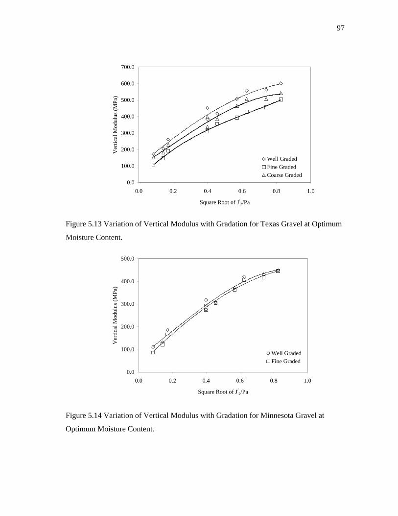
97
0.0
100.0
200.0
300.0
400.0
500.0
600.0
700.0
0.0 0.2 0.4 0.6 0.8 1.0
Square Root of J/2/Pa
Ver
tical
Mod
ulus
(MPa
)
Well GradedFine GradedCoarse Graded
Figure 5.13 Variation of Vertical Modulus with Gradation for Texas Gravel at Optimum
Moisture Content.
0.0
100.0
200.0
300.0
400.0
500.0
0.0 0.2 0.4 0.6 0.8 1.0
Square Root of J/2/Pa
Ver
tical
Mod
ulus
(MPa
)
Well GradedFine Graded
Figure 5.14 Variation of Vertical Modulus with Gradation for Minnesota Gravel at
Optimum Moisture Content.
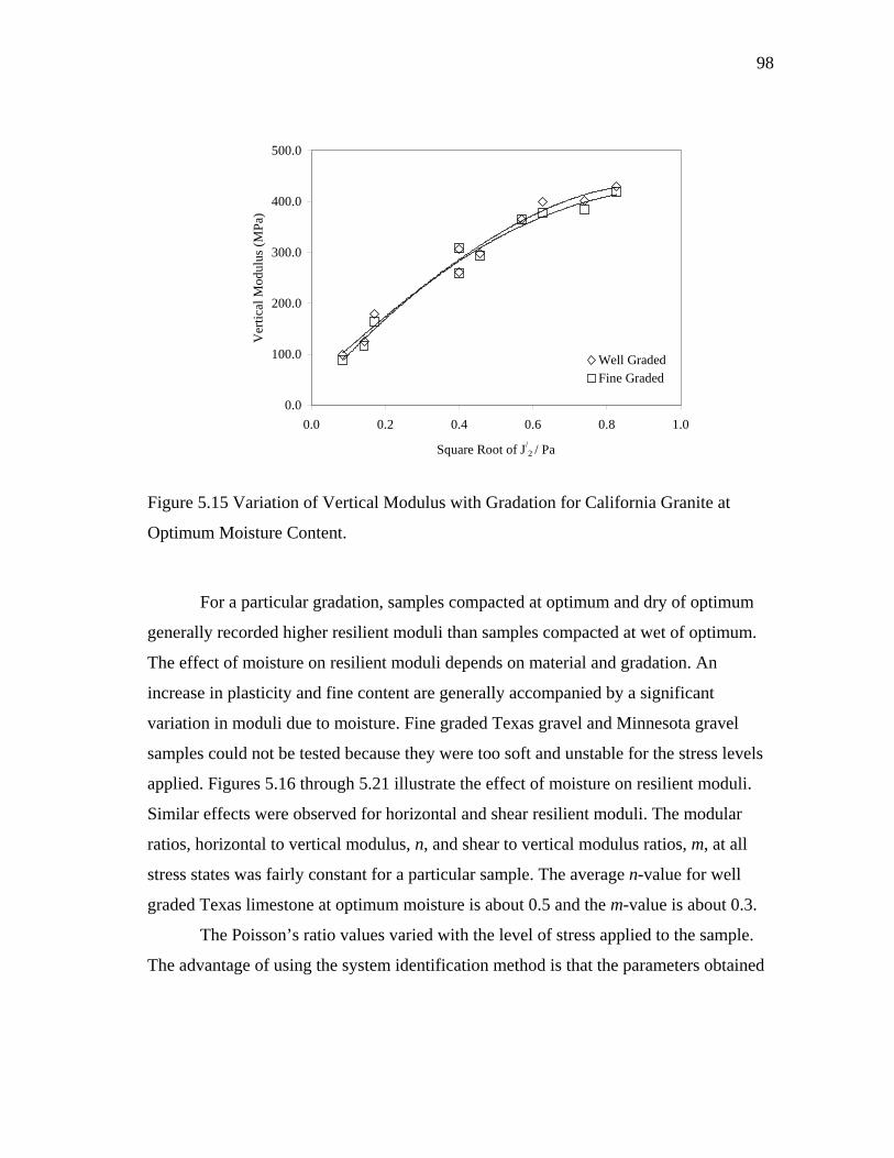
98
0.0
100.0
200.0
300.0
400.0
500.0
0.0 0.2 0.4 0.6 0.8 1.0
Square Root of J/2 / Pa
Ver
tical
Mod
ulus
(MPa
)
Well GradedFine Graded
Figure 5.15 Variation of Vertical Modulus with Gradation for California Granite at
Optimum Moisture Content.
For a particular gradation, samples compacted at optimum and dry of optimum
generally recorded higher resilient moduli than samples compacted at wet of optimum.
The effect of moisture on resilient moduli depends on material and gradation. An
increase in plasticity and fine content are generally accompanied by a significant
variation in moduli due to moisture. Fine graded Texas gravel and Minnesota gravel
samples could not be tested because they were too soft and unstable for the stress levels
applied. Figures 5.16 through 5.21 illustrate the effect of moisture on resilient moduli.
Similar effects were observed for horizontal and shear resilient moduli. The modular
ratios, horizontal to vertical modulus, n, and shear to vertical modulus ratios, m, at all
stress states was fairly constant for a particular sample. The average n-value for well
graded Texas limestone at optimum moisture is about 0.5 and the m-value is about 0.3.
The Poisson’s ratio values varied with the level of stress applied to the sample.
The advantage of using the system identification method is that the parameters obtained
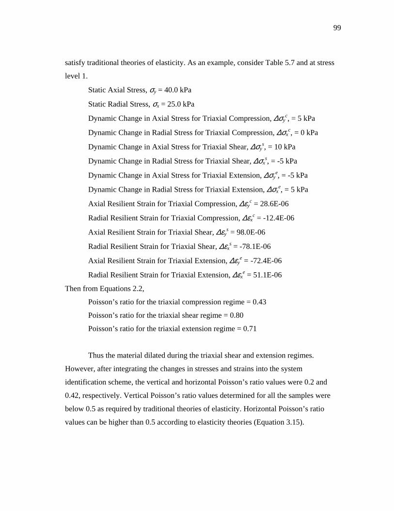
99
satisfy traditional theories of elasticity. As an example, consider Table 5.7 and at stress
level 1.
Static Axial Stress, σy = 40.0 kPa
Static Radial Stress, σx = 25.0 kPa
Dynamic Change in Axial Stress for Triaxial Compression, ∆σyc, = 5 kPa
Dynamic Change in Radial Stress for Triaxial Compression, ∆σxc, = 0 kPa
Dynamic Change in Axial Stress for Triaxial Shear, ∆σys, = 10 kPa
Dynamic Change in Radial Stress for Triaxial Shear, ∆σxs, = -5 kPa
Dynamic Change in Axial Stress for Triaxial Extension, ∆σye, = -5 kPa
Dynamic Change in Radial Stress for Triaxial Extension, ∆σxe, = 5 kPa
Axial Resilient Strain for Triaxial Compression, ∆εyc = 28.6E-06
Radial Resilient Strain for Triaxial Compression, ∆εxc = -12.4E-06
Axial Resilient Strain for Triaxial Shear, ∆εys = 98.0E-06
Radial Resilient Strain for Triaxial Shear, ∆εxs = -78.1E-06
Axial Resilient Strain for Triaxial Extension, ∆εye = -72.4E-06
Radial Resilient Strain for Triaxial Extension, ∆εxe = 51.1E-06
Then from Equations 2.2,
Poisson’s ratio for the triaxial compression regime = 0.43
Poisson’s ratio for the triaxial shear regime = 0.80
Poisson’s ratio for the triaxial extension regime = 0.71
Thus the material dilated during the triaxial shear and extension regimes.
However, after integrating the changes in stresses and strains into the system
identification scheme, the vertical and horizontal Poisson’s ratio values were 0.2 and
0.42, respectively. Vertical Poisson’s ratio values determined for all the samples were
below 0.5 as required by traditional theories of elasticity. Horizontal Poisson’s ratio
values can be higher than 0.5 according to elasticity theories (Equation 3.15).
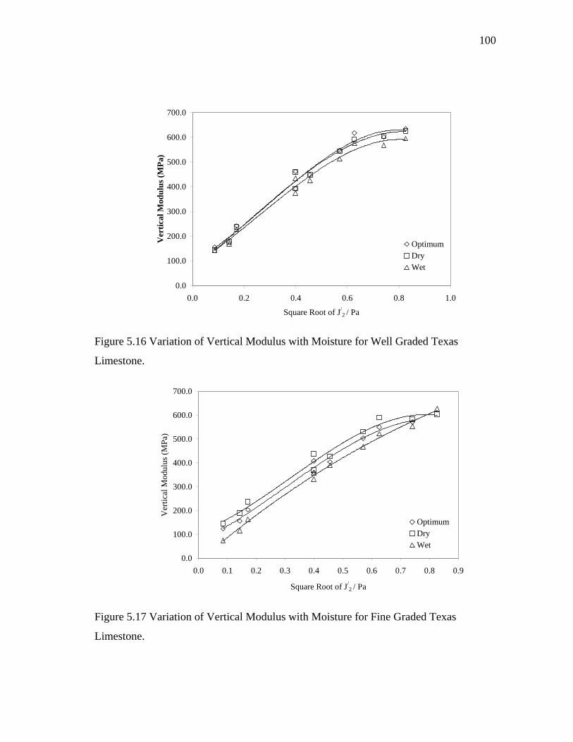
100
0.0
100.0
200.0
300.0
400.0
500.0
600.0
700.0
0.0 0.2 0.4 0.6 0.8 1.0
Square Root of J/2 / Pa
Ver
tical
Mod
ulus
(MPa
)
OptimumDryWet
Figure 5.16 Variation of Vertical Modulus with Moisture for Well Graded Texas
Limestone.
0.0
100.0
200.0
300.0
400.0
500.0
600.0
700.0
0.0 0.1 0.2 0.3 0.4 0.5 0.6 0.7 0.8 0.9
Square Root of J/2 / Pa
Ver
tical
Mod
ulus
(MPa
)
OptimumDryWet
Figure 5.17 Variation of Vertical Modulus with Moisture for Fine Graded Texas
Limestone.
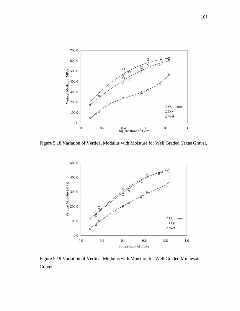
101
0.0
100.0
200.0
300.0
400.0
500.0
600.0
700.0
0 0.2 0.4 0.6 0.8 1Square Root of J/
2/Pa
Ver
tical
Mod
ulus
(MPa
)
OptimumDryWet
Figure 5.18 Variation of Vertical Modulus with Moisture for Well Graded Texas Gravel.
0.0
100.0
200.0
300.0
400.0
500.0
0.0 0.2 0.4 0.6 0.8 1.0Square Root of J/
2/Pa
Ver
tical
Mod
ulus
(MPa
)
OptimumDryWet
Figure 5.19 Variation of Vertical Modulus with Moisture for Well Graded Minnesota
Gravel.
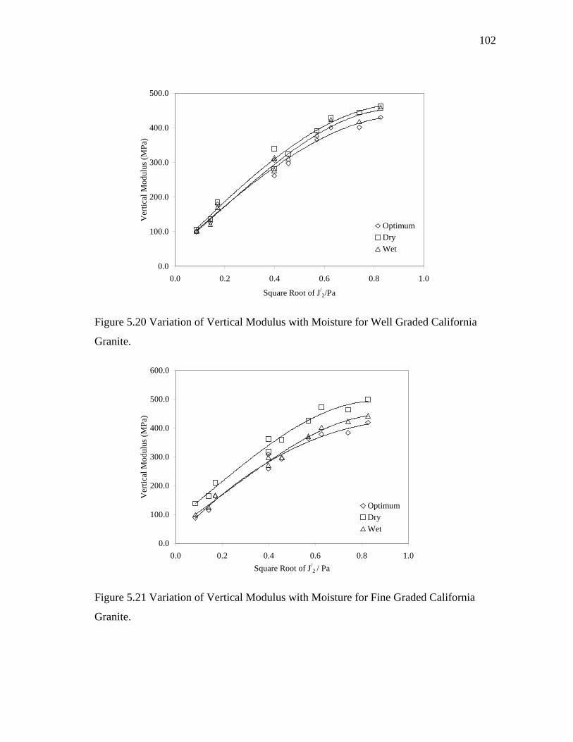
102
0.0
100.0
200.0
300.0
400.0
500.0
0.0 0.2 0.4 0.6 0.8 1.0
Square Root of J/2/Pa
Ver
tical
Mod
ulus
(MPa
)
OptimumDryWet
Figure 5.20 Variation of Vertical Modulus with Moisture for Well Graded California
Granite.
0.0
100.0
200.0
300.0
400.0
500.0
600.0
0.0 0.2 0.4 0.6 0.8 1.0Square Root of J/
2 / Pa
Ver
tical
Mod
ulus
(MPa
)
OptimumDryWet
Figure 5.21 Variation of Vertical Modulus with Moisture for Fine Graded California
Granite.
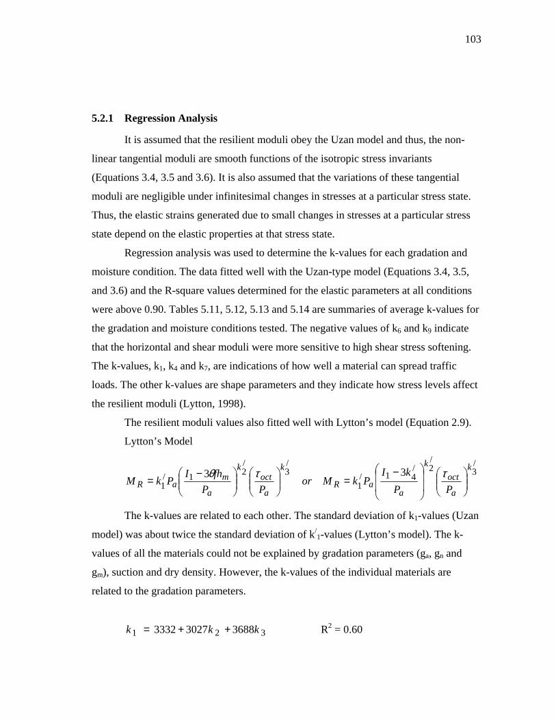
103
5.2.1 Regression Analysis
It is assumed that the resilient moduli obey the Uzan model and thus, the non-
linear tangential moduli are smooth functions of the isotropic stress invariants
(Equations 3.4, 3.5 and 3.6). It is also assumed that the variations of these tangential
moduli are negligible under infinitesimal changes in stresses at a particular stress state.
Thus, the elastic strains generated due to small changes in stresses at a particular stress
state depend on the elastic properties at that stress state.
Regression analysis was used to determine the k-values for each gradation and
moisture condition. The data fitted well with the Uzan-type model (Equations 3.4, 3.5,
and 3.6) and the R-square values determined for the elastic parameters at all conditions
were above 0.90. Tables 5.11, 5.12, 5.13 and 5.14 are summaries of average k-values for
the gradation and moisture conditions tested. The negative values of k6 and k9 indicate
that the horizontal and shear moduli were more sensitive to high shear stress softening.
The k-values, k1, k4 and k7, are indications of how well a material can spread traffic
loads. The other k-values are shape parameters and they indicate how stress levels affect
the resilient moduli (Lytton, 1998).
The resilient moduli values also fitted well with Lytton’s model (Equation 2.9).
Lytton’s Model
/3
/2/
41/1
/3
/21/
133 k
a
octk
aaR
k
a
octk
a
maR PP
kIPkMor
PPfhI
PkM
−=
−=
ττθ
The k-values are related to each other. The standard deviation of k1-values (Uzan
model) was about twice the standard deviation of k/1-values (Lytton’s model). The k-
values of all the materials could not be explained by gradation parameters (ga, gn and
gm), suction and dry density. However, the k-values of the individual materials are
related to the gradation parameters.
321 368830273332 kkk ++= R2 = 0.60
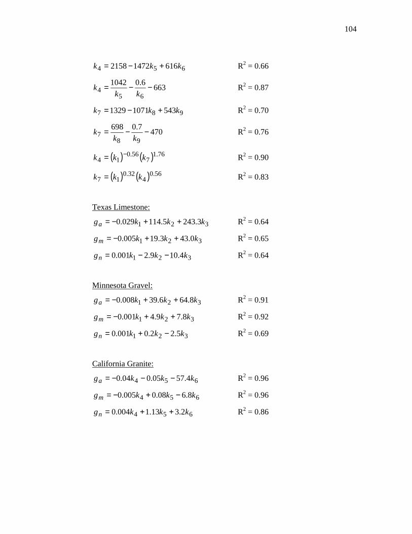
104
654 61614722158 kkk +−= R2 = 0.66
6636.01042
654 −−=
kkk R2 = 0.87
987 54310711329 kkk +−= R2 = 0.70
4707.0698
987 −−=
kkk R2 = 0.76
( ) ( ) 76.17
56.014 kkk −= R2 = 0.90
( ) ( ) 56.04
32.017 kkk = R2 = 0.83
Texas Limestone:
321 3.2435.114029.0 kkkga ++−= R2 = 0.64
321 0.433.19005.0 kkkgm ++−= R2 = 0.65
321 4.109.2001.0 kkkgn −−= R2 = 0.64
Minnesota Gravel:
321 8.646.39008.0 kkkga ++−= R2 = 0.91
321 8.79.4001.0 kkkgm ++−= R2 = 0.92
321 5.22.0001.0 kkkgn −+= R2 = 0.69
California Granite:
654 4.5705.004.0 kkkga −−−= R2 = 0.96
654 8.608.0005.0 kkkgm −+−= R2 = 0.96
654 2.313.1004.0 kkkgn ++= R2 = 0.86
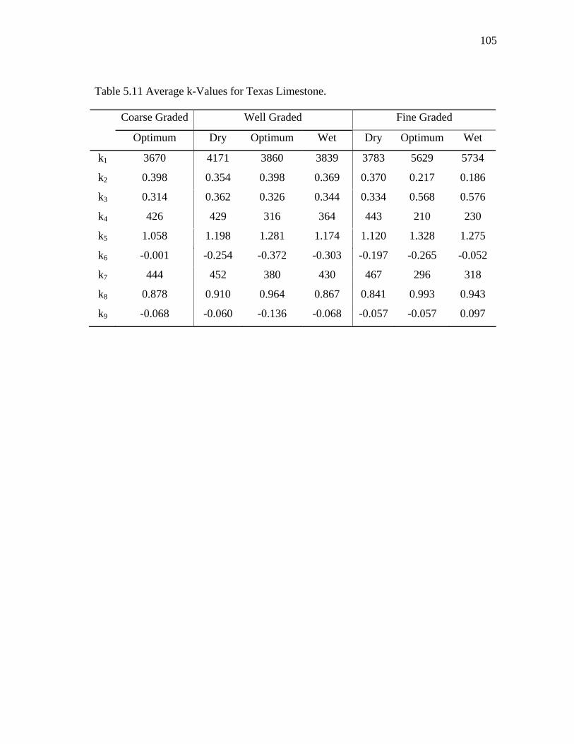
105
Table 5.11 Average k-Values for Texas Limestone.
Coarse Graded Well Graded Fine Graded
Optimum Dry Optimum Wet Dry Optimum Wet
k1 3670 4171 3860 3839 3783 5629 5734
k2 0.398 0.354 0.398 0.369 0.370 0.217 0.186
k3 0.314 0.362 0.326 0.344 0.334 0.568 0.576
k4 426 429 316 364 443 210 230
k5 1.058 1.198 1.281 1.174 1.120 1.328 1.275
k6 -0.001 -0.254 -0.372 -0.303 -0.197 -0.265 -0.052
k7 444 452 380 430 467 296 318
k8 0.878 0.910 0.964 0.867 0.841 0.993 0.943
k9 -0.068 -0.060 -0.136 -0.068 -0.057 -0.057 0.097
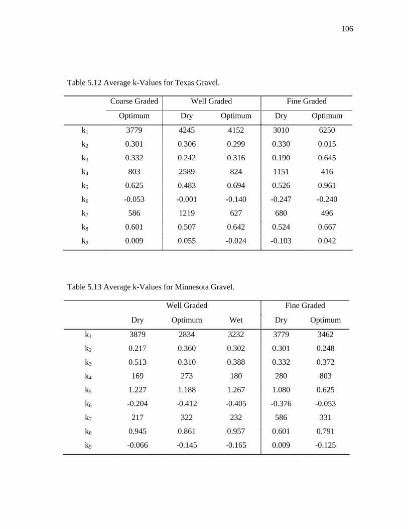
106
Table 5.12 Average k-Values for Texas Gravel.
Coarse Graded Well Graded Fine Graded
Optimum Dry Optimum Dry Optimum
k1 3779 4245 4152 3010 6250
k2 0.301 0.306 0.299 0.330 0.015
k3 0.332 0.242 0.316 0.190 0.645
k4 803 2589 824 1151 416
k5 0.625 0.483 0.694 0.526 0.961
k6 -0.053 -0.001 -0.140 -0.247 -0.240
k7 586 1219 627 680 496
k8 0.601 0.507 0.642 0.524 0.667
k9 0.009 0.055 -0.024 -0.103 0.042
Table 5.13 Average k-Values for Minnesota Gravel.
Well Graded Fine Graded
Dry Optimum Wet Dry Optimum
k1 3879 2834 3232 3779 3462
k2 0.217 0.360 0.302 0.301 0.248
k3 0.513 0.310 0.388 0.332 0.372
k4 169 273 180 280 803
k5 1.227 1.188 1.267 1.080 0.625
k6 -0.204 -0.412 -0.405 -0.376 -0.053
k7 217 322 232 586 331
k8 0.945 0.861 0.957 0.601 0.791
k9 -0.066 -0.145 -0.165 0.009 -0.125
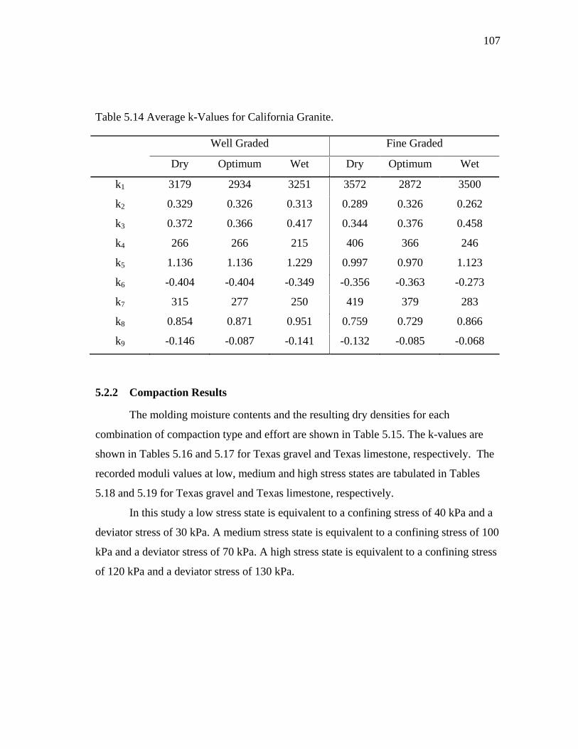
107
Table 5.14 Average k-Values for California Granite.
Well Graded Fine Graded
Dry Optimum Wet Dry Optimum Wet
k1 3179 2934 3251 3572 2872 3500
k2 0.329 0.326 0.313 0.289 0.326 0.262
k3 0.372 0.366 0.417 0.344 0.376 0.458
k4 266 266 215 406 366 246
k5 1.136 1.136 1.229 0.997 0.970 1.123
k6 -0.404 -0.404 -0.349 -0.356 -0.363 -0.273
k7 315 277 250 419 379 283
k8 0.854 0.871 0.951 0.759 0.729 0.866
k9 -0.146 -0.087 -0.141 -0.132 -0.085 -0.068
5.2.2 Compaction Results
The molding moisture contents and the resulting dry densities for each
combination of compaction type and effort are shown in Table 5.15. The k-values are
shown in Tables 5.16 and 5.17 for Texas gravel and Texas limestone, respectively. The
recorded moduli values at low, medium and high stress states are tabulated in Tables
5.18 and 5.19 for Texas gravel and Texas limestone, respectively.
In this study a low stress state is equivalent to a confining stress of 40 kPa and a
deviator stress of 30 kPa. A medium stress state is equivalent to a confining stress of 100
kPa and a deviator stress of 70 kPa. A high stress state is equivalent to a confining stress
of 120 kPa and a deviator stress of 130 kPa.
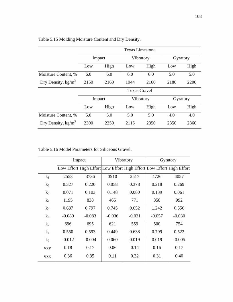
108
Table 5.15 Molding Moisture Content and Dry Density.
Texas Limestone
Impact Vibratory Gyratory
Low High Low High Low High
Moisture Content, % 6.0 6.0 6.0 6.0 5.0 5.0
Dry Density, kg/m3 2150 2160 1944 2160 2180 2200
Texas Gravel
Impact Vibratory Gyratory
Low High Low High Low High
Moisture Content, % 5.0 5.0 5.0 5.0 4.0 4.0
Dry Density, kg/m3 2300 2350 2115 2350 2350 2360
Table 5.16 Model Parameters for Siliceous Gravel.
Impact Vibratory Gyratory
Low Effort High Effort Low Effort High Effort Low Effort High Effort
k1 2553 3736 3910 2517 4726 4057
k2 0.327 0.220 0.058 0.378 0.218 0.269
k3 0.071 0.103 0.148 0.080 0.139 0.061
k4 1195 838 465 771 358 992
k5 0.637 0.797 0.745 0.652 1.242 0.556
k6 -0.089 -0.083 -0.036 -0.031 -0.057 -0.030
k7 696 695 621 559 500 754
k8 0.550 0.593 0.449 0.638 0.799 0.522
k9 -0.012 -0.004 0.060 0.019 0.019 -0.005
νxy 0.18 0.17 0.06 0.14 0.16 0.17
νxx 0.36 0.35 0.11 0.32 0.31 0.40
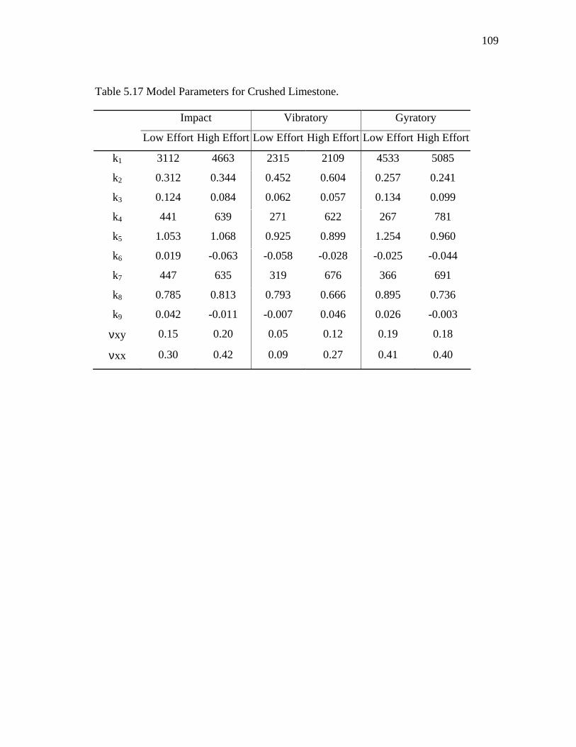
109
Table 5.17 Model Parameters for Crushed Limestone.
Impact Vibratory Gyratory
Low Effort High Effort Low Effort High Effort Low Effort High Effort
k1 3112 4663 2315 2109 4533 5085
k2 0.312 0.344 0.452 0.604 0.257 0.241
k3 0.124 0.084 0.062 0.057 0.134 0.099
k4 441 639 271 622 267 781
k5 1.053 1.068 0.925 0.899 1.254 0.960
k6 0.019 -0.063 -0.058 -0.028 -0.025 -0.044
k7 447 635 319 676 366 691
k8 0.785 0.813 0.793 0.666 0.895 0.736
k9 0.042 -0.011 -0.007 0.046 0.026 -0.003
νxy 0.15 0.20 0.05 0.12 0.19 0.18
νxx 0.30 0.42 0.09 0.27 0.41 0.40
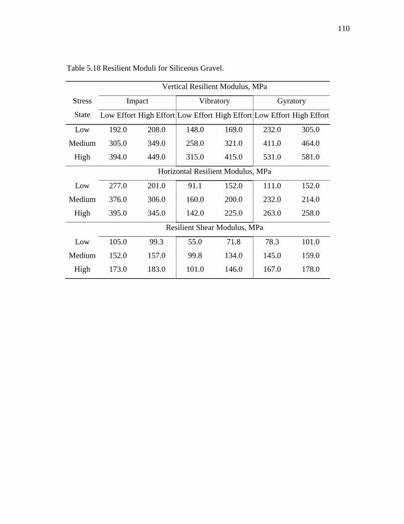
110
Table 5.18 Resilient Moduli for Siliceous Gravel.
Vertical Resilient Modulus, MPa
Impact Vibratory Gyratory Stress
State Low Effort High Effort Low Effort High Effort Low Effort High Effort
Low 192.0 208.0 148.0 169.0 232.0 305.0
Medium 305.0 349.0 258.0 321.0 411.0 464.0
High 394.0 449.0 315.0 415.0 531.0 581.0
Horizontal Resilient Modulus, MPa
Low 277.0 201.0 91.1 152.0 111.0 152.0
Medium 376.0 306.0 160.0 200.0 232.0 214.0
High 395.0 345.0 142.0 225.0 263.0 258.0
Resilient Shear Modulus, MPa
Low 105.0 99.3 55.0 71.8 78.3 101.0
Medium 152.0 157.0 99.8 134.0 145.0 159.0
High 173.0 183.0 101.0 146.0 167.0 178.0
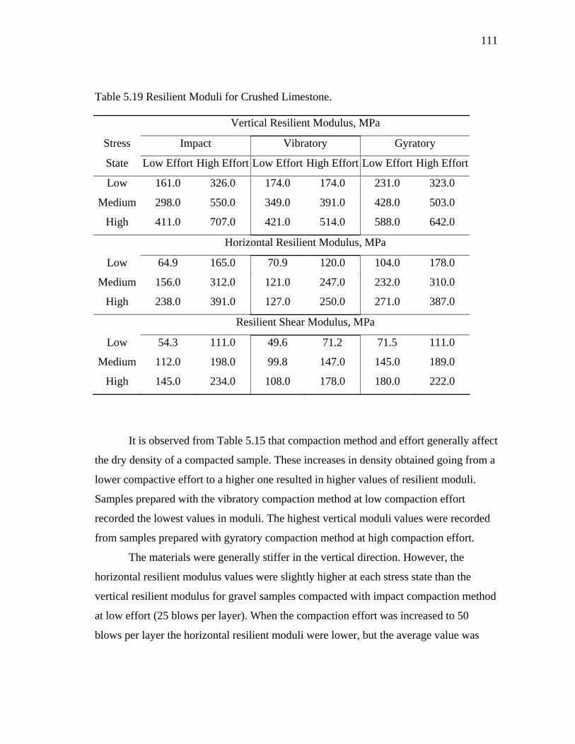
111
Table 5.19 Resilient Moduli for Crushed Limestone.
Vertical Resilient Modulus, MPa
Stress Impact Vibratory Gyratory
State Low Effort High Effort Low Effort High Effort Low Effort High Effort
Low 161.0 326.0 174.0 174.0 231.0 323.0
Medium 298.0 550.0 349.0 391.0 428.0 503.0
High 411.0 707.0 421.0 514.0 588.0 642.0
Horizontal Resilient Modulus, MPa
Low 64.9 165.0 70.9 120.0 104.0 178.0
Medium 156.0 312.0 121.0 247.0 232.0 310.0
High 238.0 391.0 127.0 250.0 271.0 387.0
Resilient Shear Modulus, MPa
Low 54.3 111.0 49.6 71.2 71.5 111.0
Medium 112.0 198.0 99.8 147.0 145.0 189.0
High 145.0 234.0 108.0 178.0 180.0 222.0
It is observed from Table 5.15 that compaction method and effort generally affect
the dry density of a compacted sample. These increases in density obtained going from a
lower compactive effort to a higher one resulted in higher values of resilient moduli.
Samples prepared with the vibratory compaction method at low compaction effort
recorded the lowest values in moduli. The highest vertical moduli values were recorded
from samples prepared with gyratory compaction method at high compaction effort.
The materials were generally stiffer in the vertical direction. However, the
horizontal resilient modulus values were slightly higher at each stress state than the
vertical resilient modulus for gravel samples compacted with impact compaction method
at low effort (25 blows per layer). When the compaction effort was increased to 50
blows per layer the horizontal resilient moduli were lower, but the average value was
112
80% of the vertical modulus as compared to 46%-60% in the case of the other
compaction methods and efforts. The degree of anisotropy is defined as the ratio of
horizontal to vertical modulus. It is assumed that the degree of anisotropy is related to
particle orientation in the unbound granular material. Thus, the induced anisotropy by
the impact compaction method was not significant. Samples compacted with the
vibratory compaction method recorded unusually low Poisson's ratios. This may be due
to the differences in LVDT range between RaTT and UIFC as mentioned earlier.
The non-linear anisotropic properties (k-values) are useful in determining
pavement response with a finite element code. The anisotropic model generally reduces
and/or reverses the horizontal tensile stresses predicted in the base course with isotropic
elastic properties. Although using impact compaction results in acceptable densities,
distribution and orientation of individual particles makes the material to behave like an
isotropic material. The orientation of particles in a compacted unbound granular material
is important to its load carrying capabilities. Further study needs to be done to establish
how the compaction methods considered are related to compaction levels achieved in the
field. Field cores of unbound granular materials should be obtained and tested in the
laboratory to confirm the observations made on compaction methods.
5.3 Permanent Deformation
The repeated load triaxial test was used to study the permanent deformation
characteristics of the four aggregate types. The permanent deformation study was
performed only on well graded samples compacted at optimum moisture.
Samples, 150-mm in height by 150-mm diameter, were compacted using the
Texas Gyratory Compactor with the high compaction effort. One sample was prepared
for each stress level because this test is destructive in nature. The permanent deformation
behavior of the materials was studied at four stress levels. At each stress level, static
confining stresses were applied to the samples and deviatoric stresses were axially
cycled for 10,000 times. A haversine pulse-load was applied for 0.1 seconds with a 0.9
seconds rest at a frequency of 1 cycle per second.
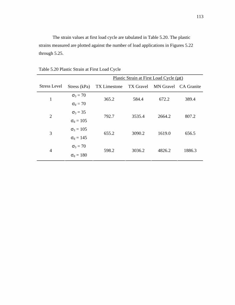
113
The strain values at first load cycle are tabulated in Table 5.20. The plastic
strains measured are plotted against the number of load applications in Figures 5.22
through 5.25.
Table 5.20 Plastic Strain at First Load Cycle
Plastic Strain at First Load Cycle (µε)
Stress Level Stress (kPa) TX Limestone TX Gravel MN Gravel CA Granite
σ3 = 70 1
σd = 70 365.2 584.4 672.2 389.4
σ3 = 35 2
σd = 105 792.7 3535.4 2664.2 807.2
σ3 = 105 3
σd = 145 655.2 3090.2 1619.0 656.5
σ3 = 70 4
σd = 180 598.2 3036.2 4826.2 1886.3
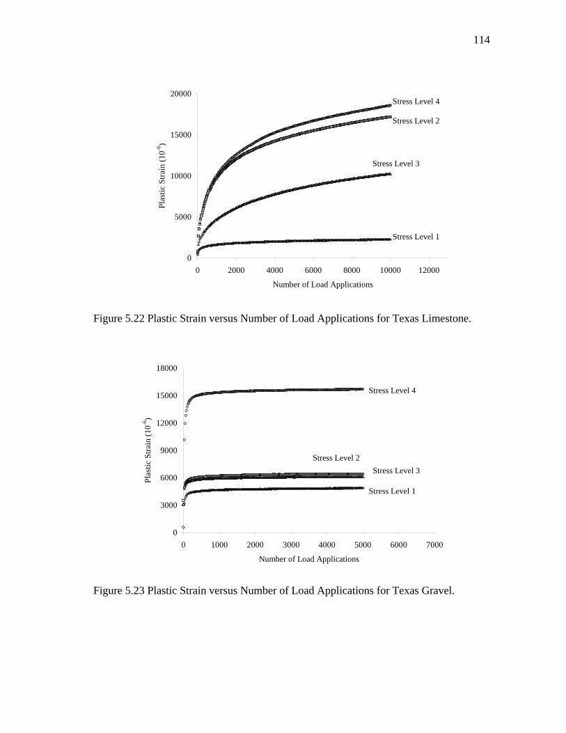
114
0
5000
10000
15000
20000
0 2000 4000 6000 8000 10000 12000
Number of Load Applications
Plas
tic S
train
(10-6
)
Stress Level 1
Stress Level 2
Stress Level 3
Stress Level 4
Figure 5.22 Plastic Strain versus Number of Load Applications for Texas Limestone.
0
3000
6000
9000
12000
15000
18000
0 1000 2000 3000 4000 5000 6000 7000
Number of Load Applications
Plas
tic S
train
(10-6
)
Stress Level 4
Stress Level 2Stress Level 3
Stress Level 1
Figure 5.23 Plastic Strain versus Number of Load Applications for Texas Gravel.
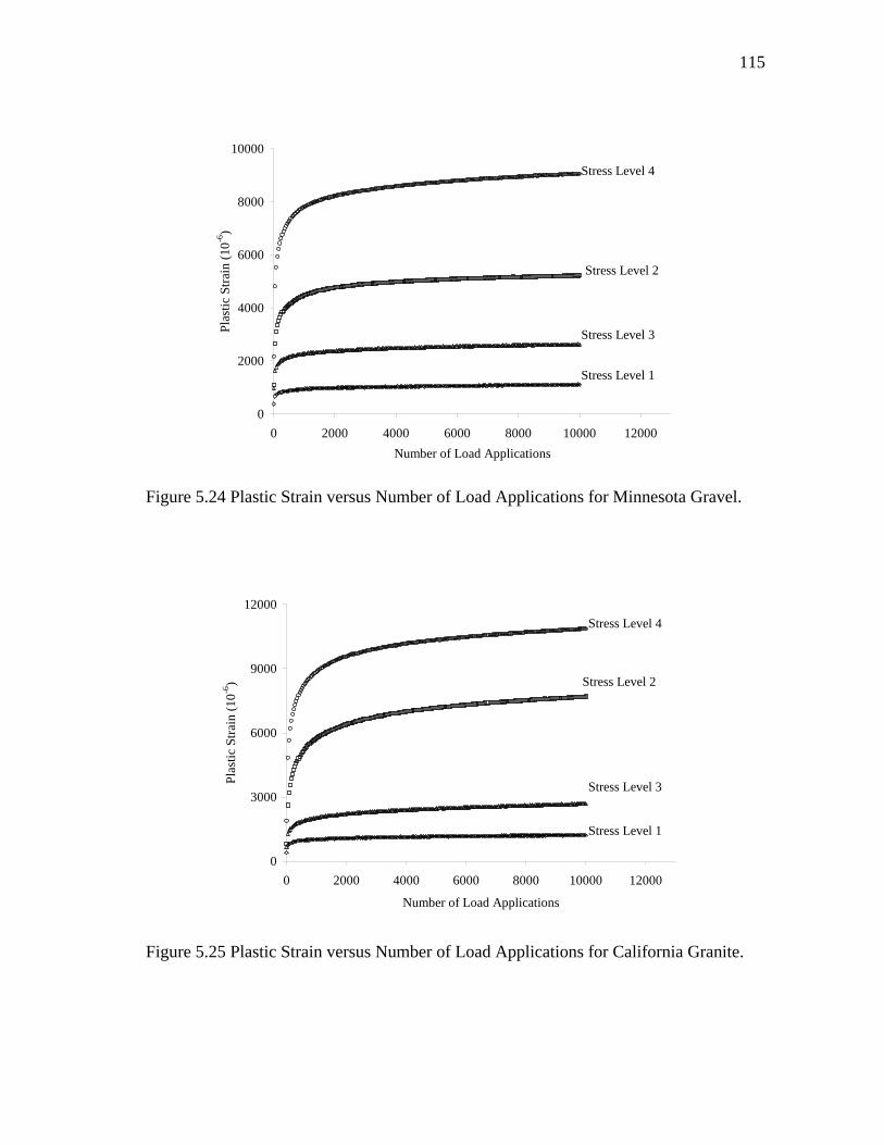
115
0
2000
4000
6000
8000
10000
0 2000 4000 6000 8000 10000 12000Number of Load Applications
Plas
tic S
train
(10-6
)
Stress Level 4
Stress Level 2
Stress Level 3
Stress Level 1
Figure 5.24 Plastic Strain versus Number of Load Applications for Minnesota Gravel.
0
3000
6000
9000
12000
0 2000 4000 6000 8000 10000 12000
Number of Load Applications
Plas
tic S
train
(10-6
)
Stress Level 4
Stress Level 2
Stress Level 3
Stress Level 1
Figure 5.25 Plastic Strain versus Number of Load Applications for California Granite.
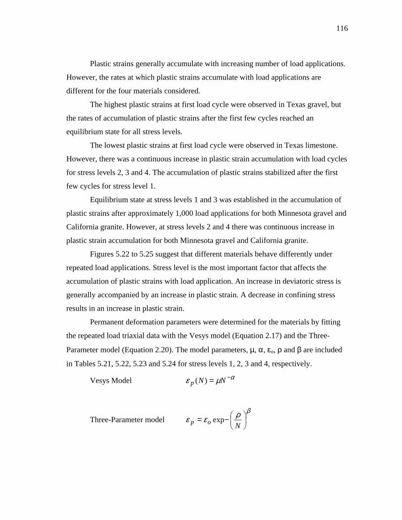
116
Plastic strains generally accumulate with increasing number of load applications.
However, the rates at which plastic strains accumulate with load applications are
different for the four materials considered.
The highest plastic strains at first load cycle were observed in Texas gravel, but
the rates of accumulation of plastic strains after the first few cycles reached an
equilibrium state for all stress levels.
The lowest plastic strains at first load cycle were observed in Texas limestone.
However, there was a continuous increase in plastic strain accumulation with load cycles
for stress levels 2, 3 and 4. The accumulation of plastic strains stabilized after the first
few cycles for stress level 1.
Equilibrium state at stress levels 1 and 3 was established in the accumulation of
plastic strains after approximately 1,000 load applications for both Minnesota gravel and
California granite. However, at stress levels 2 and 4 there was continuous increase in
plastic strain accumulation for both Minnesota gravel and California granite.
Figures 5.22 to 5.25 suggest that different materials behave differently under
repeated load applications. Stress level is the most important factor that affects the
accumulation of plastic strains with load application. An increase in deviatoric stress is
generally accompanied by an increase in plastic strain. A decrease in confining stress
results in an increase in plastic strain.
Permanent deformation parameters were determined for the materials by fitting
the repeated load triaxial data with the Vesys model (Equation 2.17) and the Three-
Parameter model (Equation 2.20). The model parameters, µ, α, εo, ρ and β are included
in Tables 5.21, 5.22, 5.23 and 5.24 for stress levels 1, 2, 3 and 4, respectively.
Vesys Model αµε −= NNp )(
Three-Parameter model βρεε
−=
Nop exp
117
Table 5.21 Permanent Deformation Parameters for Stress Level 1.
Model TX Limestone TX Gravel MN Gravel CA Granite
Parameter Vesys Model
µ 560.7 3051.9 532.3 570.3
α -0.152 -0.053 -0.080 -0.083
Three-Parameter Model
εo 8415.9 55018.0 1938.7 2184.5
ρ 160.7 E03 5.6 61.6 87.6
β 0.099 0.448 0.113 0.112
Table 5.22 Permanent Deformation Parameters for Stress Level 2.
Model TX Limestone TX Gravel MN Gravel CA Granite
Parameters Vesys Model
µ 1575.5 4837.3 2399.7 2092.2
α -0.271 -0.034 -0.087 -0.144
Three-Parameter Model
εo 65563.6 6858.5 6458.4 11788.1
ρ 32740.7 0.2 18.6 239.8
β 0.180 0.276 0.250 0.230
118
Table 5.23 Permanent Deformation Parameters for Stress Level 3.
Model TX Limestone TX Gravel MN Gravel CA Granite
Parameters Vesys Model
µ 487.9 4541.2 1356.3 854.2
α -0.332 -0.034 -0.073 -0.125
Three-Parameter Model
εo 647885.1 6457.0 3802.0 16414.2
ρ 1.85E12 0.37 10.3 158.28E6
β 0.0745 0.289 0.144 0.062
Table 5.24 Permanent Deformation Parameters for Stress Level 4.
Model TX Limestone TX Gravel MN Gravel CA Granite
Parameters Vesys Model
µ 1695.9 10702.9 4291.1 4144.9
α -0.254 -0.044 -0.083 -0.107
Three-Parameter Model
εo 36815.3 16137.6 11457.0 14775.7
ρ 3233.8 3.9 14.6 54.2
β 0.239 0.467 0.222 0.228
A small α-value indicates that the material that has low resistance to permanent
deformation (Lytton, 1998). These model parameters can be used to predict the
accumulation of permanent deformation within unbound granular layers in flexible
pavements. It is easy to determine model parameters to characterize the permanent
deformation behavior of unbound granular materials. However, the process is time
119
consuming because a new specimen has to be prepared for each stress level to eliminate
the effect of stress history.
Although the laboratory setup for characterizing permanent deformation is
simple, the levels of stresses that need to be applied must be determined accurately. This
is because stress levels, especially confining stress, have a significant impact on the rate
and magnitude of accumulation of plastic strain.
The stresses within a pavement structure can be determined by analytical
methods. Layered linear elastic methods are usually used to determine the stresses in a
pavement. The limitation of the layered elastic model is that elastic moduli must be
constant within each horizontal layer and thus, the method cannot effectively deal with
material non-linearity exhibited by unbound granular materials.
The layered elastic process can account for variation in vertical stress but cannot
effectively account for variation in lateral (confining) stresses. Since the variation of
lateral stresses within a pavement profile is as important as the variation of vertical
stresses, the finite element method (FEM) has recently been preferred to analyze
pavements. A finite element computer program was developed in this study and the
details are discussed in the next chapter.
5.3.1 Accelerated Rutting Parameters
Park (2000) developed a finite element computer program (FERUT) to predict
the accumulation of permanent deformation in granular materials. FERUT uses the
Vesys and Three Parameter models.
The formulation of the Vesys model implies that the plastic strain is an
exponential function of the number of load cycles. The Three-Parameter model states
that the plastic strain has a limit, εo, and a logarithmic rate of work hardening and also
that the plastic strain increases with the number of load applications.
One mechanism that can seriously affect the performance of unbound granular
layers is accelerated rutting due to fatigue from load repetitions. The repeated load
action of traffic does not allow the build up of pore water pressure on the soil skeleton to
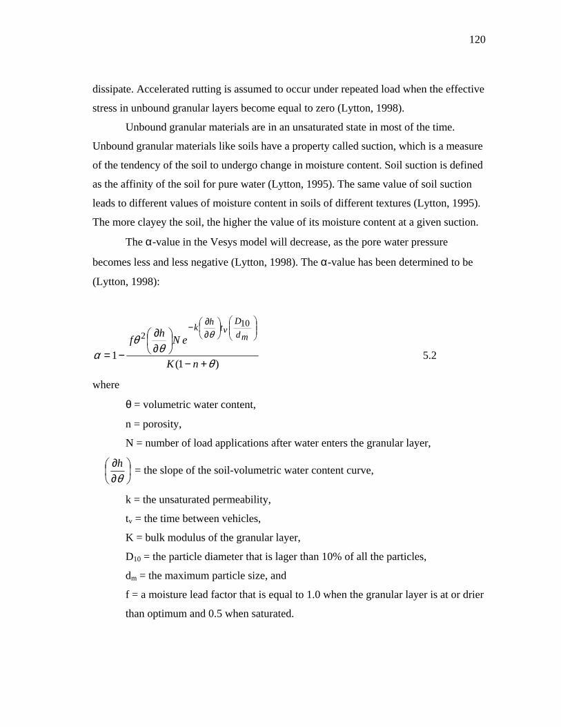
120
dissipate. Accelerated rutting is assumed to occur under repeated load when the effective
stress in unbound granular layers become equal to zero (Lytton, 1998).
Unbound granular materials are in an unsaturated state in most of the time.
Unbound granular materials like soils have a property called suction, which is a measure
of the tendency of the soil to undergo change in moisture content. Soil suction is defined
as the affinity of the soil for pure water (Lytton, 1995). The same value of soil suction
leads to different values of moisture content in soils of different textures (Lytton, 1995).
The more clayey the soil, the higher the value of its moisture content at a given suction.
The α-value in the Vesys model will decrease, as the pore water pressure
becomes less and less negative (Lytton, 1998). The α-value has been determined to be
(Lytton, 1998):
)1(1
102
θθ
θα
θ
+−
∂∂
−=
∂∂−
nK
eNhf mdD
vthk
5.2
where
θ = volumetric water content,
n = porosity,
N = number of load applications after water enters the granular layer,
∂∂θh = the slope of the soil-volumetric water content curve,
k = the unsaturated permeability,
tv = the time between vehicles,
K = bulk modulus of the granular layer,
D10 = the particle diameter that is lager than 10% of all the particles,
dm = the maximum particle size, and
f = a moisture lead factor that is equal to 1.0 when the granular layer is at or drier
than optimum and 0.5 when saturated.
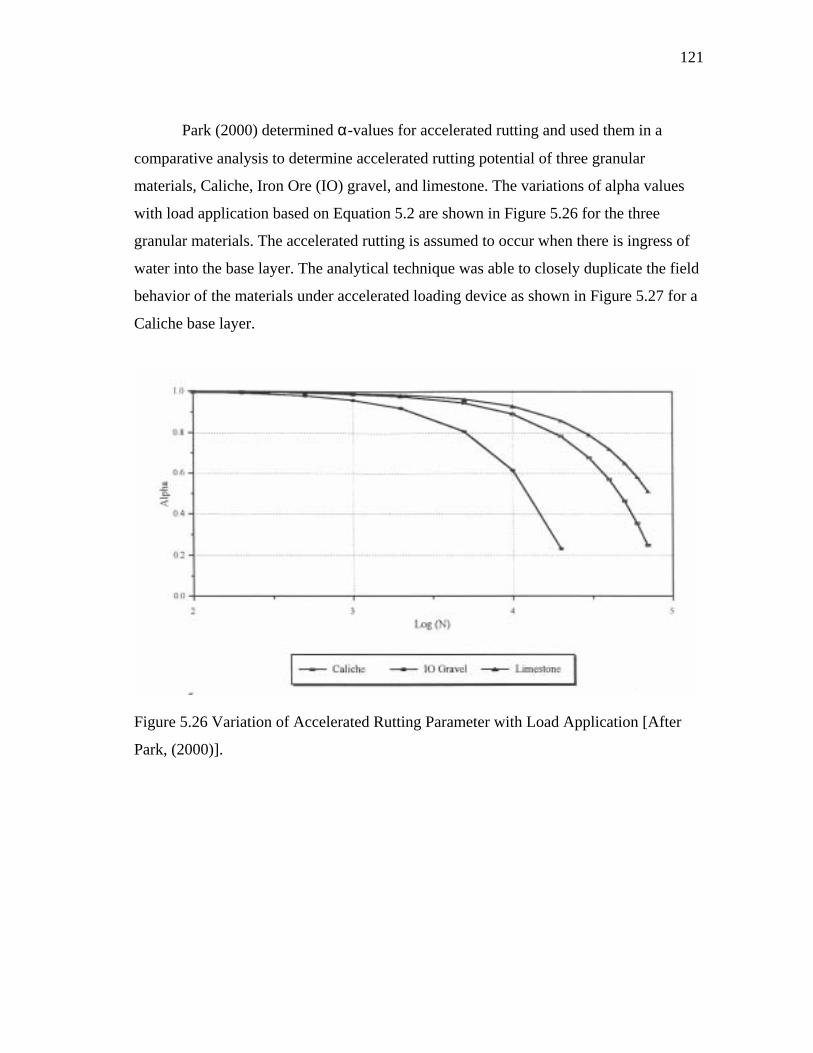
121
Park (2000) determined α-values for accelerated rutting and used them in a
comparative analysis to determine accelerated rutting potential of three granular
materials, Caliche, Iron Ore (IO) gravel, and limestone. The variations of alpha values
with load application based on Equation 5.2 are shown in Figure 5.26 for the three
granular materials. The accelerated rutting is assumed to occur when there is ingress of
water into the base layer. The analytical technique was able to closely duplicate the field
behavior of the materials under accelerated loading device as shown in Figure 5.27 for a
Caliche base layer.
Figure 5.26 Variation of Accelerated Rutting Parameter with Load Application [After
Park, (2000)].
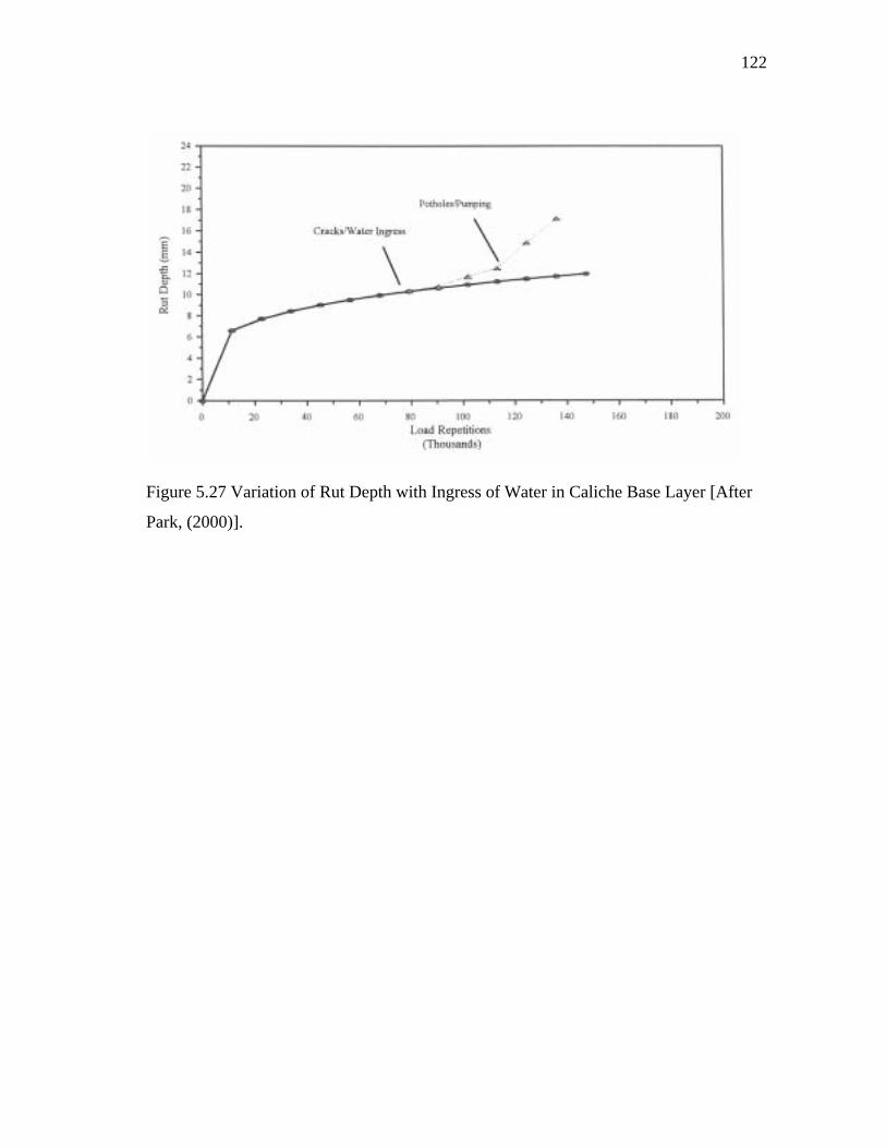
122
Figure 5.27 Variation of Rut Depth with Ingress of Water in Caliche Base Layer [After
Park, (2000)].
123
CHAPTER VI
DEVELOPMENT OF FINITE ELEMENT PROGRAM
6.1 Background
The finite element method has evolved in the past 40 years from a specialized
technique for aircraft frame analysis to a general numerical solution to a broad range of
physical problems. The historic paper written by Turner, Clough, and Topp (1956) is
credited by many for having established the method. Clough (1960) coined the term
‘finite element method’. The finite element method represents an approximate numerical
solution of a boundary-value problem described by a differential equation.
Typically engineering problems in mechanics are addressed by deriving
equations relating the variables of interest to basic principles of physics. These principles
include equilibrium, potential energy, strain energy, conservation of total energy, virtual
work, thermodynamics, conservation of mass, and many more. Finding a solution that
satisfies a differential equation throughout a region, and also yields the boundary
conditions, is a very difficult and often an impossible task for all but the most
elementary problems. The finite element method addresses this difficulty by dividing a
region into small sub-regions so that the solution within each sub-region can be
represented by a simplified function compared to that required for the entire region. The
sub-regions are joined mathematically by enforcing sub-region to sub-region boundary
compatibility while satisfying the entire region boundary requirements (Owen and
Hinton, 1980).
The finite element method is capable of including material and element non-
linearity, as well as different types of loading and interface conditions in the solution.
This highly efficient and versatile numerical technique has been applied to pavements
since the late 1960’s. However, one problem that has been identified by many
researchers (Duncan et al., 1968; Hicks, 1970) is the false prediction of horizontal tensile
stresses within unbound granular layers in flexible pavements. Unbound granular
124
materials are known to have negligible tensile strength aside from that induced by
suction and particle interlock. Therefore, they cannot accommodate the high tensile
stresses predicted. Contrary to the predicted horizontal tensile stresses, conventional
flexible pavements with granular layers have been used to carry traffic loads for decades
with a remarkable performance history.
Much research has been directed at improving pavement response models to
explain the performance of flexible pavements and to reverse the prediction of horizontal
tensile stresses in the unbound granular layers. Three primary approaches have been
used to correct the predicted horizontal tensile stresses in unbound granular layers in
flexible pavements (Tutumluer, 1995). These are:
• A no tension analysis based on stress transfer or failure envelop limitations,
• The presence of overburden and compressive residual stresses, and
• Improved constitutive models.
The stress transfer method to correct tension was proposed by Zienkiewicz et al. (1968).
In this procedure, equal compressive stresses are applied to counteract predicted
horizontal tensile stresses so that equilibrium is maintained. To improve inherent
convergence problems in the original stress transfer method, Doddihal and Pandey
(1984) modified the technique for pavements.
The Mohr-Coulomb failure envelope criterion has also been incorporated into
finite element method programs (ILLI-PAVE and MICH-PAVE) to reverse the
prediction of horizontal tensile stresses in unbound granular layers. Here, predicted
stresses are adjusted such that they remain within the Mohr-Coulomb failure envelope in
the compressive zone.
Residual compressive stresses have also been incorporated into some finite
element programs to correct predicted horizontal tensile stresses. Crockford and
Bendana (1990) and Tutumluer (1995) successfully incorporated this technique into the
TTI-PAVE and GT-PAVE finite element computer programs, respectively. It is believed
that residual stresses exist in compacted unbound granular layers. Many researchers
(Stewart et al., 1985; Uzan, 1985; Barksdale et al., 1993; Tutumluer, 1995) have
125
investigated the existence of residual stresses. The residual compressive stresses are
believed to be in the range of 13.8-kPa to 27.6-kPa (2 to 4-psi).
Some researchers have also worked on improving constitutive models used to
describe the dilation behavior of unbound granular materials. Lytton et al. (1993)
derived a differential equation describing the variation of Poisson's ratio with stress state.
The solution to this differential equation resulted in what is known as the k1-k5 model.
This model was incorporated in a finite element program (Liu, 1993) and the results
were very impressive. Cross-anisotropy has also been incorporated into finite element
programs to improve materials response in unbound granular materials (Zienkiewicz,
1966; Crockford et al., 1990; Tutumluer, 1995). After incorporating cross-anisotropic
elastic modeling in the GT-PAVE finite element code, Tutumluer (1995) reported that
cross-anisotropic elastic modeling can reduce and even reverse horizontal tensile stresses
predicted in unbound granular layers with isotropic elastic model. In his work,
Tutumluer (1995) assumed modular ratios and Poisson's ratios to satisfy strain energy
conditions.
Although the no tension correction techniques have been used successfully to
reverse predicted horizontal tensile stresses in unbound granular layers, if the
constitutive models were accurate enough, such corrections would not be necessary. This
research focused much of its attention on improving the cross-anisotropic elastic model
(Tutumluer, 1995) with stress dependent Poisson's ratios (Lytton et al., 1993; Liu, 1993).
Instead of assuming modular ratios, one of the main objectives of this study was the
development of a laboratory testing protocol for determining the anisotropic elastic
parameters of unbound granular materials. A triaxial laboratory testing protocol to
determine the five cross-anisotropic elastic parameters, which has been elusive to many
researchers until now, was developed in this study and discussed in Chapters III and IV.
6.2 Finite Element Formulation
A finite element program was developed to model a flexible pavement’s response
to traffic loads. The finite element procedures and code are derived from the elasto-
plastic formulation, originally developed by Owen and Hinton (1980). The code was
126
developed to analyze an axisymmetric problem with material non-linearity. Liu (1993)
was the first to modify the original program to analyze pavements. The modification
included mesh generation, the implementation of different constitutive models
(hypoelastic, hyperelastic, k1-k5, and elasto-plastic models), non-symmetric solutions
and the flexible boundary conditions. Park (2000) also made modifications to the code
for pavement applications. Both of these modifications included stress dependent
Poisson's ratio and non-linear analysis using load increments. The major modification
made in this research was to incorporate cross-anisotropic material properties in the code
developed by Park (2000).
The principle of virtual work can be used to formulate the finite element method.
Consider a solid body, Ω, in which the internal stresses, σ, the distributed loads per unit
volume, b, and external applied force, f, form an equilibrium field, to undergo an
arbitrary virtual displacement pattern, δ d*, which results in compatible strains, δε*, and
internal displacements, δ u*. The principle of virtual work requires that (Liu, 1993):
∫ =−−Ω
δΩδσεδ 0*)**( fddbu TTT (6.1)
The expressions for the displacements and strains within any discrete finite element are
given by (Liu, 1993):
**** dBdNu δεδδδ == (6.2)
where N is the matrix of shape functions, and B is the elastic strain matrix. Substituting
Equation 6.2 into Equation 6.1 yields:
∫ =−−Ω
δΩσδ 0*)(* fddbNBd TTTT (6.3)
The volume integration over the solid represents the sum of the individual element
contributions. Since Equation 6.3 is true for any arbitrary δd*, then (Liu, 1993);
∫ ∫ =−−Ω Ω
ΩΩσ 0bdNfdB TT (6.4)
127
Rewriting Equation 6.4 in incremental form,
∫ ∫ =−−Ω Ω
ΩΩσ 0dbdNdfddB TT (6.5)
But the incremental stress-strain relationship is given by (Liu, 1993):
CBduCd == εδσ (6.6)
where C is the material constitutive matrix. For an axisymmetric isotropic material
model, the matrix C can be written as (Tutumluer, 1995):
−−
−−
−+=
2)21(000
0)1(0)1(0)1(
)21)(1(ν
ννννννννν
ννEC (6.7)
where E is the elastic modulus and ν is the Poisson's ratio. For an axisymmetric
anisotropic material model, the C matrix is given by:
−
−+
−−
=
mPQPnPn
Pnnnnn
Pnnnnn
ACxxxyxy
xyxyxyxx
xyxyxxxy
0000)1(
0)1()(
0)()1(
2
22
22
ννννννννννν
(6.8)
where
y
xy
y
x
y
xyxx
xx
EG
m
EE
n
PQE
A
nQ
P
=
=
=
−−=
+=
)21(
)1(2νν
ν
(6.9)
Substituting Equation 6.6 into Equation 6.5 gives:
∫+=Ω
ΩdbdNdfduK TT (6.10)
128
and,
∫=Ω
ΩCBdBK TT (6.11)
In Equation 6.10, KT is the global stiffness matrix, and the displacement vector
du is the only unknown. The solution to Equation 6.5 can then be solved by conventional
matrix inversion methods. The finite element program developed uses an axisymmetric,
isoparametric 8-node elements and a 3rd order quadrature with 9 integration points
(Park, 2000). The material parameters needed for the finite element analysis are the non-
linear vertical resilient modulus k-values (k1, k2, k3), the moduli ratios (n, m) and the
value of the vertical Poisson's ratio as well as the ratio of the horizontal to vertical
Poisson's ratios. For the materials tested during this study, the moduli ratios were
different for each material but were fairly constant for a particular material at all stress
states. Based on this observation, moduli ratios were rather used as input to the finite
program instead of k1 through k9.
The vertical Poisson's ratio was assumed to be stress-dependent (Lytton et al.,
1993; Liu, 1993) as expressed by Equation (2.14):
+−+
+=
∂∂
+∂
∂21
2/2
321
2/2
3
11/2
61
311
32
I
k
J
k
I
k
J
kIIJ
xyxyxy ν
νν
A numerical solution to Equation 2.14 based on the backward difference method
was included in the finite element code by Park (2000). Park (2000) described the
numerical stepwise solution in detail.
Equation 6.5 will not generally be satisfied at any stage of computation. An
iteration algorithm is included in the program to ensure convergence. There are two
convergence criteria in the finite element program. The equilibrium criteria are based on
residual force values such that (Park, 2000):
129
TOLLER
fN
ii
N
i
ri
≤×
∑
∑
=
= 100
)(
)(
1
2
1
2ψ (6.12)
where,
N = the total number of nodal points,
r = the iteration number,
ψ = the total applied force,
f = the applied nodal force, and
TOLLER = tolerance in convergence (percent).
Park (2000) describes the equilibrium criterion in detail. In order to prevent
unreasonable predicted moduli values at low stress levels, cutoff values for both the first
stress invariant and octahedral shear stress are specified as input in the program. Also the
value of the vertical Poisson's ratio was not allowed to exceed 0.48. Although it is
common to observe Poisson's ratios above 0.5 for unbound granular materials in the
laboratory, the presence of confinement in field conditions prompted the use of 0.48 as
the maximum vertical Poisson's ratio.
The finite element program was used to analyze a set of pavement sections. The
unbound granular base layers were modeled as linear isotropic, nonlinear isotropic,
linear anisotropic and nonlinear anisotropic.
6.3 Pavement Analysis
The elasto-plastic finite element solutions have been observed to be unstable and
divergent when the friction angle of a material is greater than 50º (Liu, 1993). Since the
friction angle of unbound granular materials can be greater than 50º, the Uzan's non-
linear elastic model (Equation 2.8) was implemented in the finite element program
instead of the elasto-plastic model.
130
Uzan Model: 32
11
k
a
octk
aaR PP
IPkE
=
τ
The formulation of Equation 2.8 is general. It can easily be downgraded to a
linear elastic model when the material parameters, k2, and k3 are set to zero. Apart from
the non-linear material parameters, the modular ratios (n, m) and the ratio of horizontal
to vertical Poisson's ratio (µ) are needed as input parameters.
where:
y
xEE
n = ,
y
xy
EG
n = , and
xy
xxννµ =
A matrix of 27 different pavement sections was analyzed using the finite element
program. The pavement sections were selected to investigate the effect of layer
thicknesses and subgrade moduli on pavement response using different constitutive
models within the unbound granular base course. The pavement matrix is a combination
of 50-, 100-, and 150-mm thick hot mix asphalt (HMA) layers on 150-, 300-, and 450-
mm thick base courses resting on sub-grades with stiffness of 20.7-, 103.4-, and 206.8-
MPa. The pavement structure is shown in Figure 6.1. A standard wheel load of 40 kN
was modeled on the surface of each pavement. The loads are assumed to be uniformly
distributed over circular areas with radii of 136-mm each.
The pavements were analyzed using linear isotropic, non-linear isotropic, linear
anisotropic and non-linear anisotropic constitutive models for the base course. The base
material properties used in the analysis are those of a well-graded crushed limestone,
compacted at optimum moisture. For all the pavements analyzed in the matrix, the HMA
layers and sub-grades were assumed to be non-linear isotropic. Thus, a total of 108
computer runs were performed using the finite element program to predict the
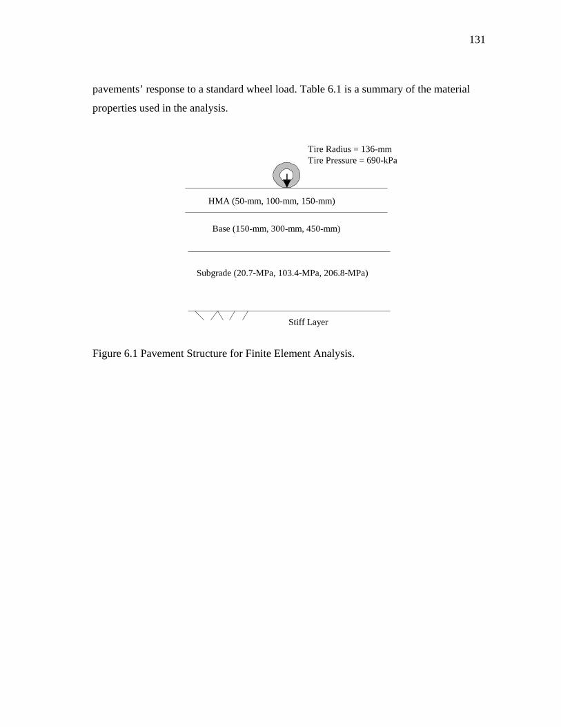
131
pavements’ response to a standard wheel load. Table 6.1 is a summary of the material
properties used in the analysis.
HMA (50-mm, 100-mm, 150-mm)
Base (150-mm, 300-mm, 450-mm)
Subgrade (20.7-MPa, 103.4-MPa, 206.8-MPa)
Tire Radius = 136-mmTire Pressure = 690-kPa
Stiff Layer
Figure 6.1 Pavement Structure for Finite Element Analysis.
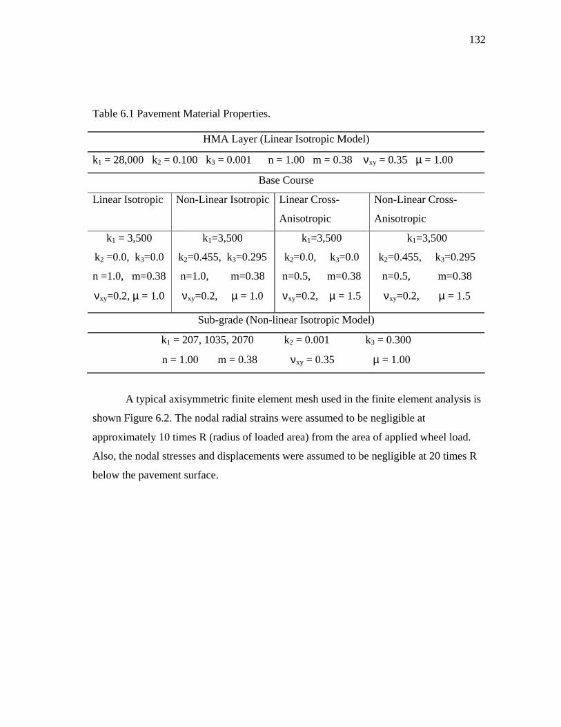
132
Table 6.1 Pavement Material Properties.
HMA Layer (Linear Isotropic Model)
k1 = 28,000 k2 = 0.100 k3 = 0.001 n = 1.00 m = 0.38 νxy = 0.35 µ = 1.00
Base Course
Linear Isotropic Non-Linear Isotropic Linear Cross-
Anisotropic
Non-Linear Cross-
Anisotropic
k1 = 3,500
k2 =0.0, k3=0.0
n =1.0, m=0.38
νxy=0.2, µ = 1.0
k1=3,500
k2=0.455, k3=0.295
n=1.0, m=0.38
νxy=0.2, µ = 1.0
k1=3,500
k2=0.0, k3=0.0
n=0.5, m=0.38
νxy=0.2, µ = 1.5
k1=3,500
k2=0.455, k3=0.295
n=0.5, m=0.38
νxy=0.2, µ = 1.5
Sub-grade (Non-linear Isotropic Model)
k1 = 207, 1035, 2070 k2 = 0.001 k3 = 0.300
n = 1.00 m = 0.38 νxy = 0.35 µ = 1.00
A typical axisymmetric finite element mesh used in the finite element analysis is
shown Figure 6.2. The nodal radial strains were assumed to be negligible at
approximately 10 times R (radius of loaded area) from the area of applied wheel load.
Also, the nodal stresses and displacements were assumed to be negligible at 20 times R
below the pavement surface.
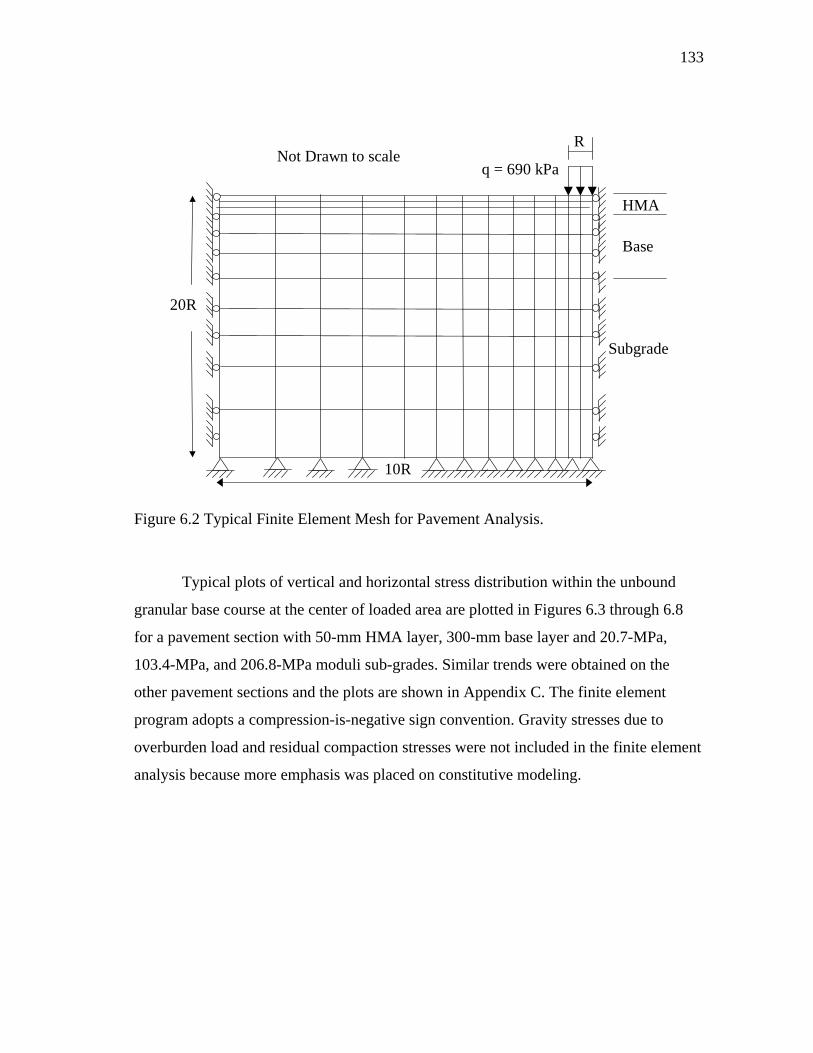
133
HMA
Base
Subgrade
Not Drawn to scaleR
20R
10R
q = 690 kPa
Figure 6.2 Typical Finite Element Mesh for Pavement Analysis.
Typical plots of vertical and horizontal stress distribution within the unbound
granular base course at the center of loaded area are plotted in Figures 6.3 through 6.8
for a pavement section with 50-mm HMA layer, 300-mm base layer and 20.7-MPa,
103.4-MPa, and 206.8-MPa moduli sub-grades. Similar trends were obtained on the
other pavement sections and the plots are shown in Appendix C. The finite element
program adopts a compression-is-negative sign convention. Gravity stresses due to
overburden load and residual compaction stresses were not included in the finite element
analysis because more emphasis was placed on constitutive modeling.
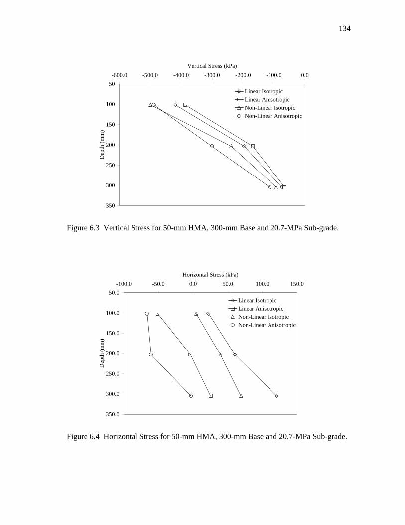
134
50
100
150
200
250
300
350
-600.0 -500.0 -400.0 -300.0 -200.0 -100.0 0.0Vertical Stress (kPa)
Dep
th (m
m)
Linear IsotropicLinear AnisotropicNon-Linear IsotropicNon-Linear Anisotropic
Figure 6.3 Vertical Stress for 50-mm HMA, 300-mm Base and 20.7-MPa Sub-grade.
50.0
100.0
150.0
200.0
250.0
300.0
350.0
-100.0 -50.0 0.0 50.0 100.0 150.0Horizontal Stress (kPa)
Dep
th (m
m)
Linear IsotropicLinear AnisotropicNon-Linear IsotropicNon-Linear Anisotropic
Figure 6.4 Horizontal Stress for 50-mm HMA, 300-mm Base and 20.7-MPa Sub-grade.
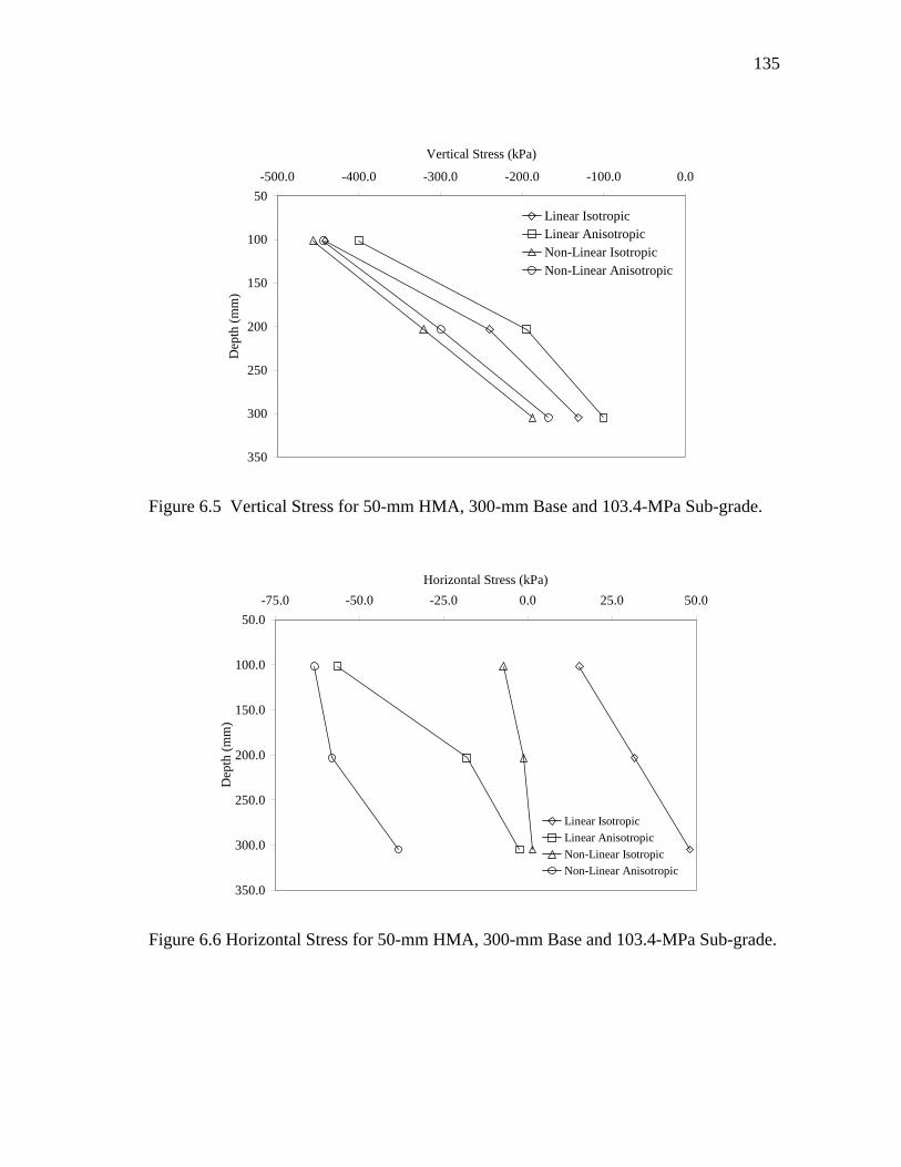
135
50
100
150
200
250
300
350
-500.0 -400.0 -300.0 -200.0 -100.0 0.0
Vertical Stress (kPa)
Dep
th (m
m)
Linear IsotropicLinear AnisotropicNon-Linear IsotropicNon-Linear Anisotropic
Figure 6.5 Vertical Stress for 50-mm HMA, 300-mm Base and 103.4-MPa Sub-grade.
50.0
100.0
150.0
200.0
250.0
300.0
350.0
-75.0 -50.0 -25.0 0.0 25.0 50.0Horizontal Stress (kPa)
Dep
th (m
m)
Linear IsotropicLinear AnisotropicNon-Linear IsotropicNon-Linear Anisotropic
Figure 6.6 Horizontal Stress for 50-mm HMA, 300-mm Base and 103.4-MPa Sub-grade.
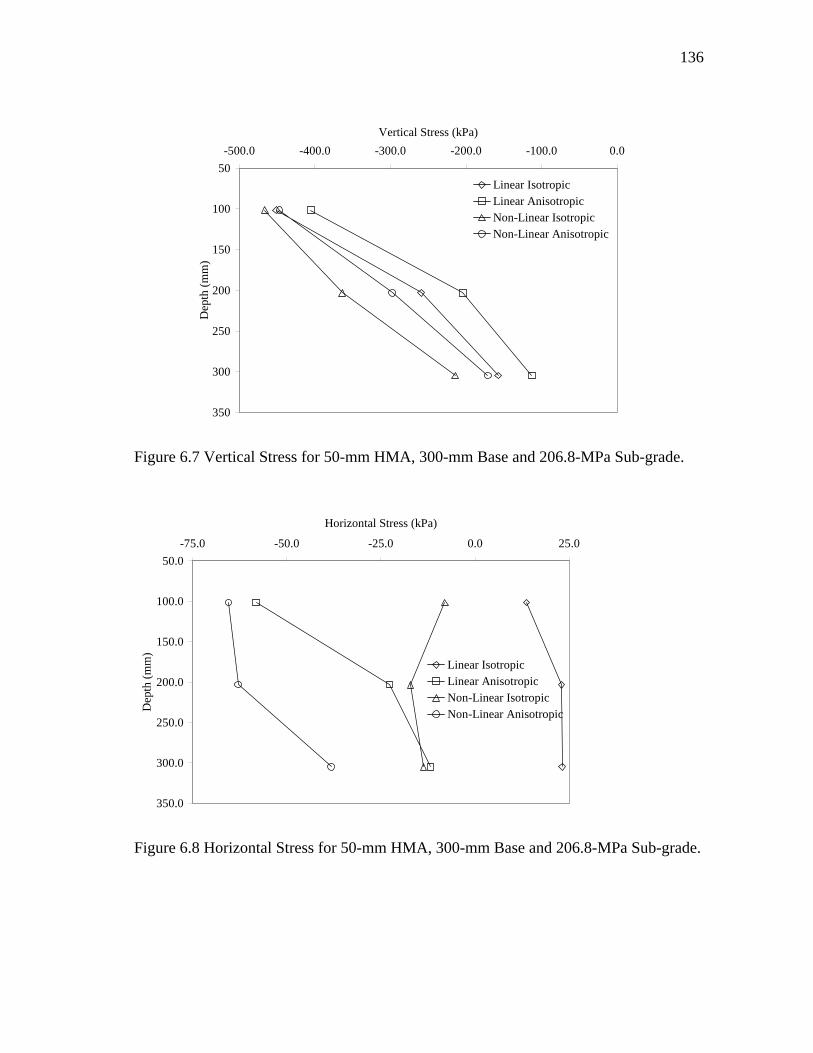
136
50
100
150
200
250
300
350
-500.0 -400.0 -300.0 -200.0 -100.0 0.0Vertical Stress (kPa)
Dep
th (m
m)
Linear IsotropicLinear AnisotropicNon-Linear IsotropicNon-Linear Anisotropic
Figure 6.7 Vertical Stress for 50-mm HMA, 300-mm Base and 206.8-MPa Sub-grade.
50.0
100.0
150.0
200.0
250.0
300.0
350.0
-75.0 -50.0 -25.0 0.0 25.0
Horizontal Stress (kPa)
Dep
th (m
m)
Linear IsotropicLinear AnisotropicNon-Linear IsotropicNon-Linear Anisotropic
Figure 6.8 Horizontal Stress for 50-mm HMA, 300-mm Base and 206.8-MPa Sub-grade.
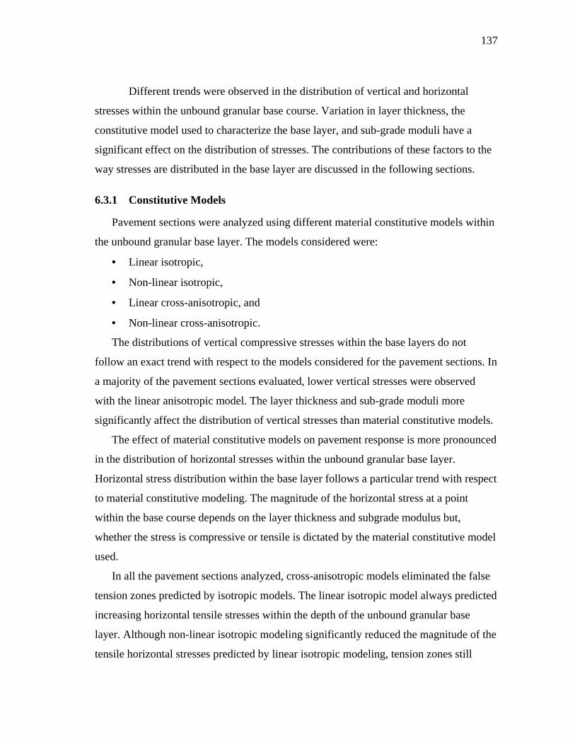
137
Different trends were observed in the distribution of vertical and horizontal
stresses within the unbound granular base course. Variation in layer thickness, the
constitutive model used to characterize the base layer, and sub-grade moduli have a
significant effect on the distribution of stresses. The contributions of these factors to the
way stresses are distributed in the base layer are discussed in the following sections.
6.3.1 Constitutive Models
Pavement sections were analyzed using different material constitutive models within
the unbound granular base layer. The models considered were:
• Linear isotropic,
• Non-linear isotropic,
• Linear cross-anisotropic, and
• Non-linear cross-anisotropic.
The distributions of vertical compressive stresses within the base layers do not
follow an exact trend with respect to the models considered for the pavement sections. In
a majority of the pavement sections evaluated, lower vertical stresses were observed
with the linear anisotropic model. The layer thickness and sub-grade moduli more
significantly affect the distribution of vertical stresses than material constitutive models.
The effect of material constitutive models on pavement response is more pronounced
in the distribution of horizontal stresses within the unbound granular base layer.
Horizontal stress distribution within the base layer follows a particular trend with respect
to material constitutive modeling. The magnitude of the horizontal stress at a point
within the base course depends on the layer thickness and subgrade modulus but,
whether the stress is compressive or tensile is dictated by the material constitutive model
used.
In all the pavement sections analyzed, cross-anisotropic models eliminated the false
tension zones predicted by isotropic models. The linear isotropic model always predicted
increasing horizontal tensile stresses within the depth of the unbound granular base
layer. Although non-linear isotropic modeling significantly reduced the magnitude of the
tensile horizontal stresses predicted by linear isotropic modeling, tension zones still
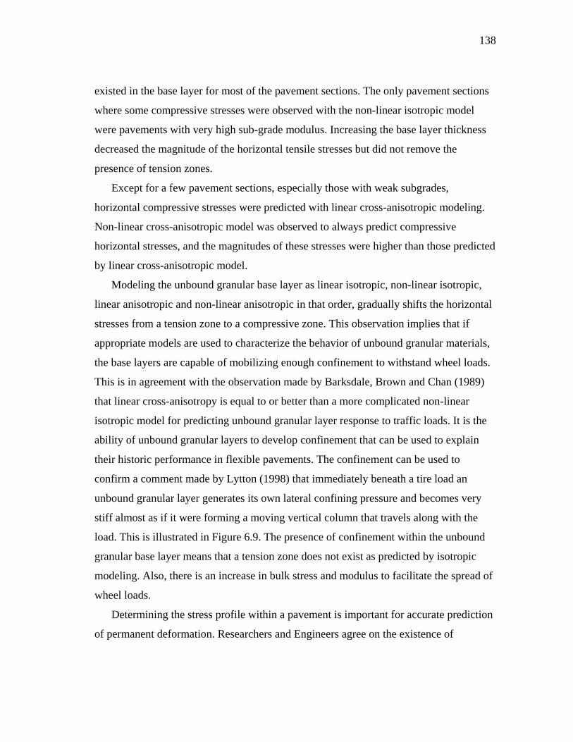
138
existed in the base layer for most of the pavement sections. The only pavement sections
where some compressive stresses were observed with the non-linear isotropic model
were pavements with very high sub-grade modulus. Increasing the base layer thickness
decreased the magnitude of the horizontal tensile stresses but did not remove the
presence of tension zones.
Except for a few pavement sections, especially those with weak subgrades,
horizontal compressive stresses were predicted with linear cross-anisotropic modeling.
Non-linear cross-anisotropic model was observed to always predict compressive
horizontal stresses, and the magnitudes of these stresses were higher than those predicted
by linear cross-anisotropic model.
Modeling the unbound granular base layer as linear isotropic, non-linear isotropic,
linear anisotropic and non-linear anisotropic in that order, gradually shifts the horizontal
stresses from a tension zone to a compressive zone. This observation implies that if
appropriate models are used to characterize the behavior of unbound granular materials,
the base layers are capable of mobilizing enough confinement to withstand wheel loads.
This is in agreement with the observation made by Barksdale, Brown and Chan (1989)
that linear cross-anisotropy is equal to or better than a more complicated non-linear
isotropic model for predicting unbound granular layer response to traffic loads. It is the
ability of unbound granular layers to develop confinement that can be used to explain
their historic performance in flexible pavements. The confinement can be used to
confirm a comment made by Lytton (1998) that immediately beneath a tire load an
unbound granular layer generates its own lateral confining pressure and becomes very
stiff almost as if it were forming a moving vertical column that travels along with the
load. This is illustrated in Figure 6.9. The presence of confinement within the unbound
granular base layer means that a tension zone does not exist as predicted by isotropic
modeling. Also, there is an increase in bulk stress and modulus to facilitate the spread of
wheel loads.
Determining the stress profile within a pavement is important for accurate prediction
of permanent deformation. Researchers and Engineers agree on the existence of
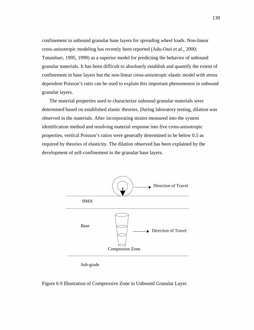
139
confinement in unbound granular base layers for spreading wheel loads. Non-linear
cross-anisotropic modeling has recently been reported (Adu-Osei et al., 2000;
Tutumluer, 1995, 1999) as a superior model for predicting the behavior of unbound
granular materials. It has been difficult to absolutely establish and quantify the extent of
confinement in base layers but the non-linear cross-anisotropic elastic model with stress
dependent Poisson’s ratio can be used to explain this important phenomenon in unbound
granular layers.
The material properties used to characterize unbound granular materials were
determined based on established elastic theories. During laboratory testing, dilation was
observed in the materials. After incorporating strains measured into the system
identification method and resolving material response into five cross-anisotropic
properties, vertical Poisson’s ratios were generally determined to be below 0.5 as
required by theories of elasticity. The dilation observed has been explained by the
development of self-confinement in the granular base layers.
Direction of Travel
Direction of Travel
HMA
Base
Sub-grade
Compresion Zone
Figure 6.9 Illustration of Compressive Zone in Unbound Granular Layer.
140
6.3.2 Layer Thickness
For a given base layer thickness and subgrade modulus, increasing the thickness
of the HMA layer decreases the magnitude of the vertical and horizontal stresses at any
point in the base layer. Similar trends were observed in increasing the base layer
thickness for a given HMA layer and sub-grade modulus.
Increasing the HMA or base layer thickness did not explain the existence of
tension or compression zone in the unbound granular base layer. Thus the design
philosophy in which the thickness of the unbound granular base layer is increased until
the tension zone, as predicted by isotropic elastic methods, diminishes is very
conservative. This design practice would result in pavement sections that are much
thicker than needed.
6.3.3 Subgrade Modulus
The subgrade moduli values of 20.7-, 103.4-, and 206.8-MPa used in this study
represent a weak, strong, and chemically stabilized subgrade, respectively. Increasing
the subgrade modulus did not significantly change the distribution of vertical stresses
within the base layer.
For a given pavement section, an increase in subgrade modulus did not
significantly change the horizontal compressive stresses predicted with the non-linear
cross-anisotropic model. However, the following were observed for the other material
models:
• Increasing the subgrade modulus shifted the few tension zones in the base layer
predicted by the linear cross-anisotropic model into compression zones.
• Increasing subgrade modulus shifted most of the tension zones in the base layer
predicted by the non-linear isotropic model into compression zones.
• Although the magnitudes of the stresses in the tension zones in the base layer
predicted by linear isotropic modeling were significantly reduced, increasing the
subgrade modulus did not remove the presence of tension zones in the base layer
141
It must also be noted that the magnitudes of the horizontal compressive stresses
predicted by the linear cross-anisotropic and non-linear isotropic models, as a result of
subgrade improvement, were still lower than the stresses predicted by the non-linear
cross-anisotropic model.
The higher compressive stresses predicted by the nonlinear cross-anisotropic
model predicts not only a stiffer base course under load but also the potential for
accelerated rutting due to ingress of water and an incremental build-up of pore water
pressure with repeated traffic loading. This tendency will be greater in those base
courses with higher percent of fines (Lytton, 1998).
142
CHAPTER VII
FIELD VALIDATION OF RESILIENT RESPONSE
7.1 Background
The cross-anisotropic resilient model developed in this study was verified with
field data collected on two pavement sections at the TTI Research Annex. The data used
in the field validation was originally collected in a study conducted by Uzan and
Scullion (1990) to verify backcalculation procedures. The pavement sections were
instrumented with Multi-Depth Deflectometers (MDD). Falling Weight Deflectometer
(FWD) loads were applied to the pavement surfaces and pavement response (deflections)
were collected. Pavement deflections were determined with the finite element program
developed in this study and compared to deflections measured in the field. The effect of
using different material models to characterize unbound granular layers on deflections
was also studied.
The National Institute for Transport and Road Research (NITRR) in South Africa
developed the MDD (Basson, 1981; Scullion et al., 1988). It is used to measure the
resilient deflection and permanent deformation in pavement layers. Figure 7.1 is a
schematic diagram of the MDD sensor. The MDD consists of modules with LVDTs that
are positioned at different depths in the pavement to measure vertical movement in the
layers. A maximum of six MDD sensors may be located in a single hole. The field
installation and calibration are described elsewhere (Basson, 1981; Scullion et al., 1988).
The two pavement sections have different layer thicknesses. Section 11 has a thin
surfacing over a thick crushed limestone base over a sandy gravel subgrade. Section 12
has a thick surface layer over a thick crushed limestone base over a sandy gravel
subgrade. The MDD anchors are located at 1.625 and 2.025 meters in the thin and thick
sections, respectively. The thin pavement had two MDD sensors and the thick pavement
had four. The pavement layer thicknesses and MDD sensor locations are shown in
Figure 7.2.
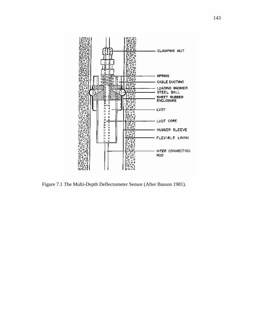
143
Figure 7.1 The Multi-Depth Deflectometer Sensor (After Basson 1981).
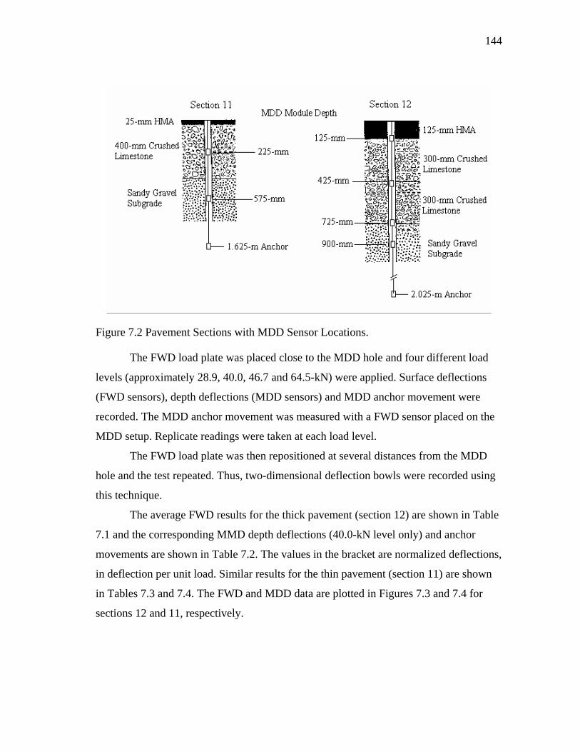
144
Figure 7.2 Pavement Sections with MDD Sensor Locations.
The FWD load plate was placed close to the MDD hole and four different load
levels (approximately 28.9, 40.0, 46.7 and 64.5-kN) were applied. Surface deflections
(FWD sensors), depth deflections (MDD sensors) and MDD anchor movement were
recorded. The MDD anchor movement was measured with a FWD sensor placed on the
MDD setup. Replicate readings were taken at each load level.
The FWD load plate was then repositioned at several distances from the MDD
hole and the test repeated. Thus, two-dimensional deflection bowls were recorded using
this technique.
The average FWD results for the thick pavement (section 12) are shown in Table
7.1 and the corresponding MMD depth deflections (40.0-kN level only) and anchor
movements are shown in Table 7.2. The values in the bracket are normalized deflections,
in deflection per unit load. Similar results for the thin pavement (section 11) are shown
in Tables 7.3 and 7.4. The FWD and MDD data are plotted in Figures 7.3 and 7.4 for
sections 12 and 11, respectively.
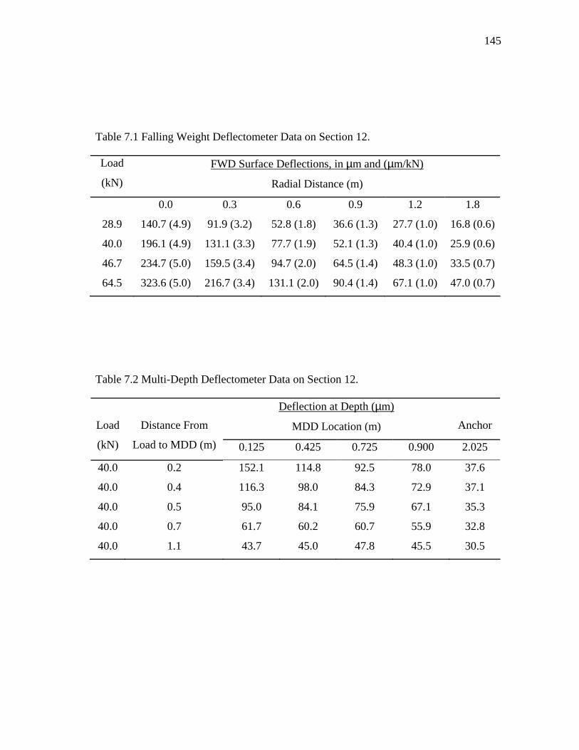
145
Table 7.1 Falling Weight Deflectometer Data on Section 12.
Load
(kN)
FWD Surface Deflections, in µm and (µm/kN)
Radial Distance (m)
0.0 0.3 0.6 0.9 1.2 1.8
28.9 140.7 (4.9) 91.9 (3.2) 52.8 (1.8) 36.6 (1.3) 27.7 (1.0) 16.8 (0.6)
40.0 196.1 (4.9) 131.1 (3.3) 77.7 (1.9) 52.1 (1.3) 40.4 (1.0) 25.9 (0.6)
46.7 234.7 (5.0) 159.5 (3.4) 94.7 (2.0) 64.5 (1.4) 48.3 (1.0) 33.5 (0.7)
64.5 323.6 (5.0) 216.7 (3.4) 131.1 (2.0) 90.4 (1.4) 67.1 (1.0) 47.0 (0.7)
Table 7.2 Multi-Depth Deflectometer Data on Section 12.
Deflection at Depth (µm)
MDD Location (m)
Anchor
Load
(kN)
Distance From
Load to MDD (m) 0.125 0.425 0.725 0.900 2.025
40.0 0.2 152.1 114.8 92.5 78.0 37.6
40.0 0.4 116.3 98.0 84.3 72.9 37.1
40.0 0.5 95.0 84.1 75.9 67.1 35.3
40.0 0.7 61.7 60.2 60.7 55.9 32.8
40.0 1.1 43.7 45.0 47.8 45.5 30.5
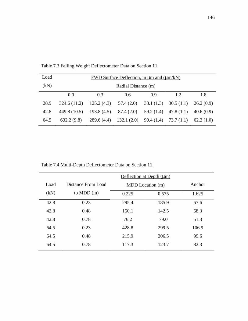
146
Table 7.3 Falling Weight Deflectometer Data on Section 11.
Load
(kN)
FWD Surface Deflection, in µm and (µm/kN)
Radial Distance (m)
0.0 0.3 0.6 0.9 1.2 1.8
28.9 324.6 (11.2) 125.2 (4.3) 57.4 (2.0) 38.1 (1.3) 30.5 (1.1) 26.2 (0.9)
42.8 449.8 (10.5) 193.8 (4.5) 87.4 (2.0) 59.2 (1.4) 47.8 (1.1) 40.6 (0.9)
64.5 632.2 (9.8) 289.6 (4.4) 132.1 (2.0) 90.4 (1.4) 73.7 (1.1) 62.2 (1.0)
Table 7.4 Multi-Depth Deflectometer Data on Section 11.
Deflection at Depth (µm)
MDD Location (m)
Anchor
Load
(kN)
Distance From Load
to MDD (m) 0.225 0.575 1.625
42.8 0.23 295.4 185.9 67.6
42.8 0.48 150.1 142.5 68.3
42.8 0.78 76.2 79.0 51.3
64.5 0.23 428.8 299.5 106.9
64.5 0.48 215.9 206.5 99.6
64.5 0.78 117.3 123.7 82.3
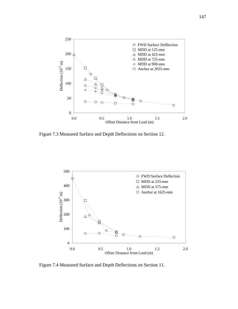
147
0
50
100
150
200
250
0.0 0.5 1.0 1.5 2.0Offset Distance from Load (m)
Def
lect
ion
(10-6
m)
FWD Surface DefllectionMDD at 125-mmMDD at 425-mmMDD at 725-mmMDD at 900-mmAnchor at 2025-mm
Figure 7.3 Measured Surface and Depth Deflections on Section 12.
0
100
200
300
400
500
0.0 0.5 1.0 1.5 2.0Offset Distance from Load (m)
Def
lect
ion
(10-6
m)
FWD Surface DeflectionMDD at 225-mmMDD at 575-mmAnchor at 1625-mm
Figure 7.4 Measured Surface and Depth Deflections on Section 11.
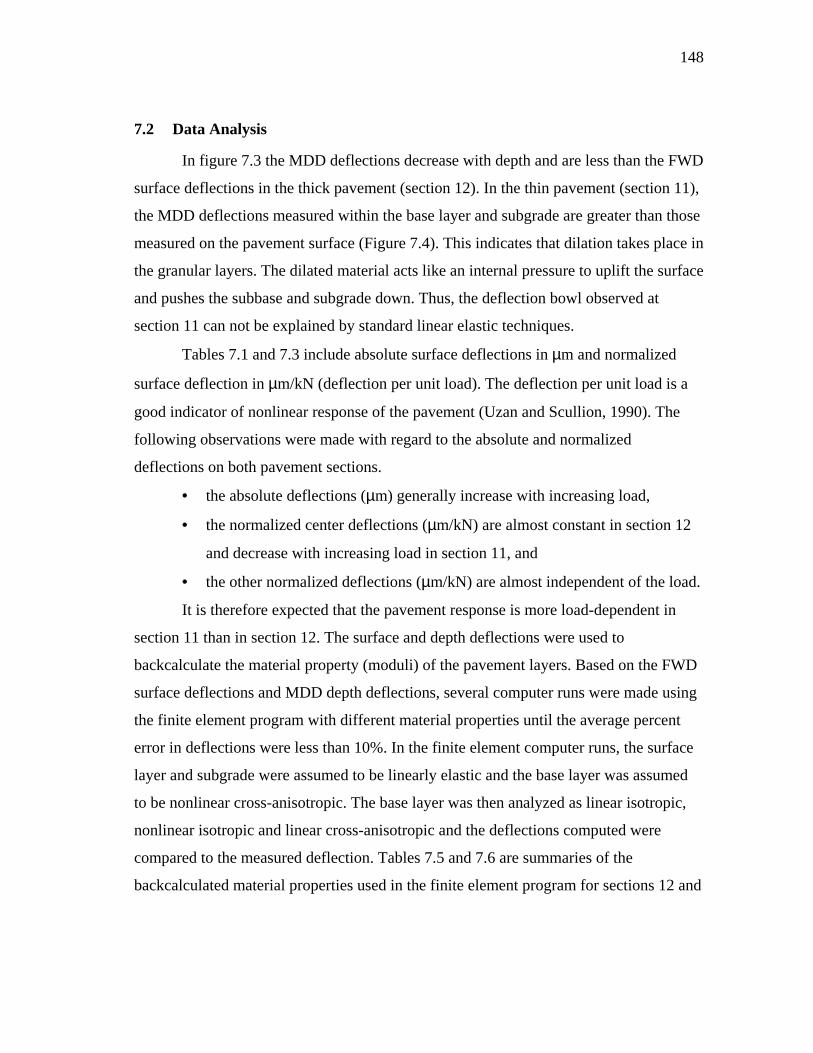
148
7.2 Data Analysis
In figure 7.3 the MDD deflections decrease with depth and are less than the FWD
surface deflections in the thick pavement (section 12). In the thin pavement (section 11),
the MDD deflections measured within the base layer and subgrade are greater than those
measured on the pavement surface (Figure 7.4). This indicates that dilation takes place in
the granular layers. The dilated material acts like an internal pressure to uplift the surface
and pushes the subbase and subgrade down. Thus, the deflection bowl observed at
section 11 can not be explained by standard linear elastic techniques.
Tables 7.1 and 7.3 include absolute surface deflections in µm and normalized
surface deflection in µm/kN (deflection per unit load). The deflection per unit load is a
good indicator of nonlinear response of the pavement (Uzan and Scullion, 1990). The
following observations were made with regard to the absolute and normalized
deflections on both pavement sections.
• the absolute deflections (µm) generally increase with increasing load,
• the normalized center deflections (µm/kN) are almost constant in section 12
and decrease with increasing load in section 11, and
• the other normalized deflections (µm/kN) are almost independent of the load.
It is therefore expected that the pavement response is more load-dependent in
section 11 than in section 12. The surface and depth deflections were used to
backcalculate the material property (moduli) of the pavement layers. Based on the FWD
surface deflections and MDD depth deflections, several computer runs were made using
the finite element program with different material properties until the average percent
error in deflections were less than 10%. In the finite element computer runs, the surface
layer and subgrade were assumed to be linearly elastic and the base layer was assumed
to be nonlinear cross-anisotropic. The base layer was then analyzed as linear isotropic,
nonlinear isotropic and linear cross-anisotropic and the deflections computed were
compared to the measured deflection. Tables 7.5 and 7.6 are summaries of the
backcalculated material properties used in the finite element program for sections 12 and
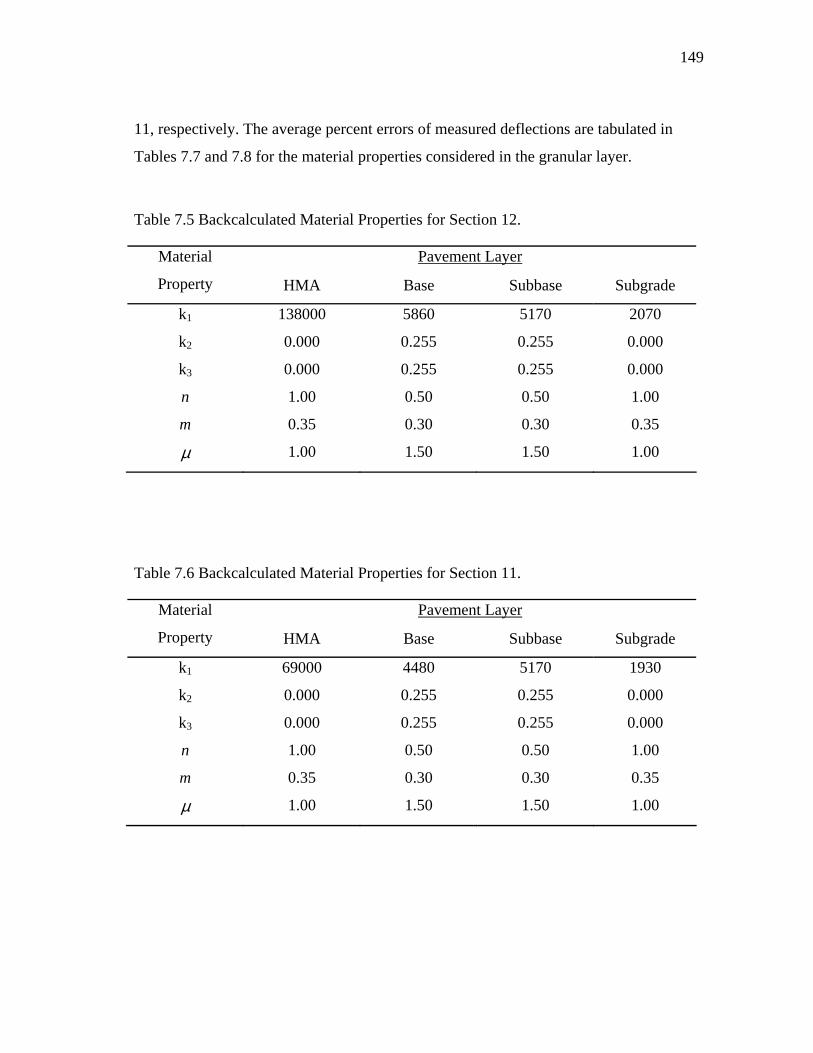
149
11, respectively. The average percent errors of measured deflections are tabulated in
Tables 7.7 and 7.8 for the material properties considered in the granular layer.
Table 7.5 Backcalculated Material Properties for Section 12.
Pavement Layer Material
Property HMA Base Subbase Subgrade
k1 138000 5860 5170 2070
k2 0.000 0.255 0.255 0.000
k3 0.000 0.255 0.255 0.000
n 1.00 0.50 0.50 1.00
m 0.35 0.30 0.30 0.35
µ 1.00 1.50 1.50 1.00
Table 7.6 Backcalculated Material Properties for Section 11.
Pavement Layer Material
Property HMA Base Subbase Subgrade
k1 69000 4480 5170 1930
k2 0.000 0.255 0.255 0.000
k3 0.000 0.255 0.255 0.000
n 1.00 0.50 0.50 1.00
m 0.35 0.30 0.30 0.35
µ 1.00 1.50 1.50 1.00
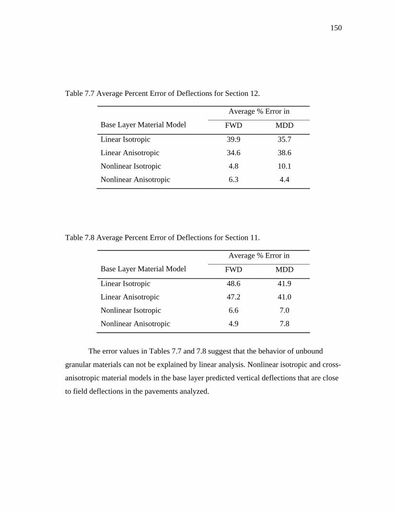
150
Table 7.7 Average Percent Error of Deflections for Section 12.
Average % Error in
Base Layer Material Model FWD MDD
Linear Isotropic 39.9 35.7
Linear Anisotropic 34.6 38.6
Nonlinear Isotropic 4.8 10.1
Nonlinear Anisotropic 6.3 4.4
Table 7.8 Average Percent Error of Deflections for Section 11.
Average % Error in
Base Layer Material Model FWD MDD
Linear Isotropic 48.6 41.9
Linear Anisotropic 47.2 41.0
Nonlinear Isotropic 6.6 7.0
Nonlinear Anisotropic 4.9 7.8
The error values in Tables 7.7 and 7.8 suggest that the behavior of unbound
granular materials can not be explained by linear analysis. Nonlinear isotropic and cross-
anisotropic material models in the base layer predicted vertical deflections that are close
to field deflections in the pavements analyzed.
151
CHAPTER VIII
CONCLUSIONS AND RECOMMENDATIONS
8.1 Conclusions
An apparent anisotropy is induced in an unbound granular layer during
construction, becoming stiffer in the vertical direction than in the horizontal direction
even before traffic loads impose further anisotropy.
Existing pavement design and analysis methods rely on empirical procedures
which have generally taken a very conservative view of the relative strength properties
of granular materials used as base and subbase layers in conventional flexible
pavements. The contribution of unbound granular layers to the overall structural
integrity of flexible pavements is significant, especially for thinly surfaced low volume
roads.
Until particulate mechanics are developed to a level where it can reasonably be
applied to characterize unbound granular materials, nonlinear and cross-anisotropic
models can be used to characterize the behavior of granular materials in pavements.
There is strong evidence in the literature that nonlinear cross-anisotropic elastic
models are superior to isotropic models in characterizing granular materials. However, it
has been extremely difficult to determine the cross-anisotropic material properties of
unbound granular materials using the conventional triaxial setup.
A laboratory testing protocol has been developed to determine the cross-
anisotropic material properties of unbound granular materials in flexible pavements. The
testing protocol was developed based on theories of elasticity. The protocol uses three
incremental stress regimes in ten stress levels to determine stress sensitivity and cross-
anisotropy. A system identification method is used as an analytical technique to compute
the five cross-anisotropic material properties. The material properties, once determined
from the testing protocol satisfy the requirements elastic work potential.
152
The testing protocol is an excellent tool for both unbound granular material
characterization and comparative analysis of materials. A compaction study on two very
different granular materials (rounded river gravel and crushed limestone) was performed
in which the aggregates were subjected to impact and gyratory shear compaction. The
level of anisotropy in a material is assumed to depend on particle orientation. The
differences in the tendency of the compaction method to produce varying levels of
particle orientation, which affects anisotropy was evident in the degree of anisotropy
measured.
Samples used in this study were compacted for height to diameter ratios of 1:1.
This is contrary to the conventional height to diameter ratios of 2:1 used in triaxial
testing. The resilient behavior of 1:1 and 2:1 samples were studied. It was observed that
difference in sample size did not significantly affect the resilient behavior of the samples
tested.
The resilient and permanent deformation behaviors of four granular materials
were studied. Material type, gradation, moisture content and stress levels affect the
deformation of granular materials. The effect of moisture on resilient moduli depends on
material type and gradation. An increase in plasticity and fine content is generally
accompanied by a significant variation in moduli due to changes in moisture content.
The moduli ratios, horizontal to vertical modulus, n, and shear to vertical
modulus ratios, m, were fairly constant for a particular material at all stress levels. The
Poisson’s ratio values varied with the level of stress applied to the sample. Instead of
using k1 through k9 coefficients to describe a granular material, the moduli and Poisson’s
ratios, together with k1, k2 and can be used. This way, there is no need to write separate
subroutines for the convergence of horizontal and shear resilient moduli in the finite
element program. Once a subroutine is written for the convergence of vertical resilient
modulus, the moduli ratios (m and n) account for the convergence of horizontal and
shear resilient moduli.
Nonlinear regression analysis was used to obtain good fits of the resilient moduli
with Uzan and Lytton models. The R-square determined for each material was above
153
0.90. Regression coefficients, which indicate how well a material can spread traffic
loads, were obtained. The regression coefficients are related.
The permanent deformation data was used to fit the Vesys and Three-Parameter
models. Model parameters, which indicate the permanent deformation potential of each
material, were obtained.
Different granular materials behave differently under repeated loading. At low
stress levels, accumulation of permanent deformation may stabilize. At high stress levels
however, plastic strains will continuously accumulate. Applied stress levels have
significant effect on how permanent strains will accumulate with repeated loading.
Although it is easy to study the permanent deformation behavior of granular materials in
the laboratory, it is important that stress levels expected in the field be applied to
laboratory samples.
Existing analytical techniques use layered elastic procedures, which fall short of
accurately predicting horizontal stresses in flexible pavements. A finite element program
was modified to incorporate nonlinear cross-anisotropic material behavior and stress
dependent Poisson’s ratio. Different pavement sections were analyzed with the finite
element program. Nonlinear cross-anisotropic modeling was observed to predict self-
confinement within granular layers.
The resilient model was validated with data collected form the field. Finite
element runs were performed on pavement sections and it was observed that linear
elastic modeling was not adequate to explain the behavior unbound granular layers. The
errors in measured pavement deflections predicted using nonlinear cross-anisotropic and
isotropic models in the base layers were less than 10%.
8.2 Recommendations
In the development of the testing protocol it was assumed that the material would
behave linearly elastic under small stress changes. The stress changes used in the stress
regimes were small and do not simulate the stress path under a moving wheel load. It is
recommended that larger stress changes be used and compared to the small changes used
in this study.
154
Further testing needs to be done on other granular materials to confirm the
general-purpose nature of the system identification method to analyze laboratory data.
More instrumented pavement sections need to be built to obtain a large field
database for further validation of the finite element program. Existing modulus
backcalculation methods use linear layered elastic techniques. It is extremely difficult to
use finite element methods to backcalculate layer material properties. Further research
needs to be done to incorporate material non-linearity in backcalculation methods to
account for the behavior of unbound granular layers.
Further study needs to be done to establish how the compaction methods
considered are related to compaction levels achieved in the field. Undisturbed field cores
of unbound granular materials must be obtained and tested in the laboratory to confirm
the material properties and the observations made on compaction methods.
155
REFERENCES
American Association of State and Highway Officials (AASHTO). (1993). “AASHTO
Guide for Design of Pavement Structures.” American Association of State and
Highway Officials Washington DC.
Adu-Osei, A., Lytton, R. L. and Little D. N. (2000). “System Identification Method for
Determining the Anisotropic Resilient Properties of Unbound Aggregates.”
Unbound Aggregates in Roads (UNBAR5) Symposium, University of Nottingham,
England, June 21-23, 2000.
Alavi, S. H. (1992). “Viscoelastic and Permanent Deformation Characteristics of
Asphalt-Aggregate Mixes Tested as Hollow Cylinders and Subjected to Dynamic
Axial and Shear Loads.” Ph.D. Thesis, University of California, Berkely, CA.
Allen, J. J. (1973). “The effects of Non-Constant Lateral Pressures on Resilient
Response of Granular Materials.” Ph.D. Dissertation. University of Illinois at
Urbana-Champaign, Il.
Allen, J. J. and Thompson, M. R. (1974). “Resilient Response of Granular Materials
Subjected to Time Dependent Lateral Stresses.” Transportation Research Record
510, Transportation Research Board, Washington, DC, 173-182.
Alvin, R. G. and Ulery, H. H. (1962). “Tabulated Values for Determining the Complete
Pattern of Stresses, Strains and Deflections Beneath A Uniform Circular Load on a
Homogeneous Half Space.” Bulletin 342, Highway Research Board, 1-13.
Amadei, B. (1983). “Rock Anisotropy and the Theory of Stress Measurements.” Lecture
Notes in Engineering; 2. Springer-Verlag.
Barksdale, R. D. (1971). “Compressive Pulse Times in Flexible Pavements for Use in
Dynamic Testing.” Highway Research Record No. 345, Highway Research Board,
National Research Council, Washington, DC.
Barksdale, R. D. (1972). “Laboratory Evaluation of Rutting in Base Course Materials.”
Proceedings, 3rd International Conference on the Structural Design of Asphalt
Pavements, Vol. 1, Ann Arbor, MI, 161-174.
156
Barksdale, R. D. (1991). “The Aggregate Handbook.” National Stone Association,
Washington D.C. Mercury Publishing Services, MD.
Barksdale, R. D. and Alba, J. L. (1993). “Laboratory Determination of Resilient
Modulus for Flexible Pavement Design.” Interim Report No. 2, NCHRP,
Transportation Research Board, National Research Council, Washington, DC.
Barksdale, R. D., Brown, S. F. and Chan, F. (1989). “Potential Benefits of Geosynthetics
in Flexible Pavements.” NCHRP Report 315, Transportation Research Council,
Washington, DC.
Bishop, A. W. and Green, G. E. (1965). “The Influence of End Restraint on the
Compression Strength of a Cohesionless Soil.” Geotechnique, Vol. 15, No. 3, 243-
265.
Boussinesq, J. (1885). “Application des Potentiels a L’etude de L’equilibre et du
Mouvement des Solids Elastiques.” Gauthier-Villars, Paris.
Boyce, J. R. (1976). “The Behavior of a Granular Material Under Repeated Load.” Ph.D.
Thesis, University of Nottingham, Department of Civil Engineering, U.K.
Boyce, J. R., Brown, S. F. and Pell, P. S. (1976). “The resilient Behaviour of a Granular
Material Under Repeated Loading.” Proceedings, Australia Road Research Board,
28, 8-19.
Brown, S. F. (1996). “Soil Mechanics in Pavement Engineering.” Geotechnique Vol. 46,
No. 3, 383-426.
Brown, S. F., O’Reilly, M. P., and Pappin, J. W. (1989). “A Repeated Load Triaxial
Apparatus for granular Materials.” Unbound Aggregates in Roads, London,
Butterworth, 143-158.
Burmister, D. M. (1943). “The Theory of Stresses and Displacements in Layered
Systems and Applications to the Design of Airport Runways.” Proceedings,
Highway Research Board, Vol. 23, 126-144.
157
Burmister, D. M. (1945). “The General Theory of Stresses and Displacements in
Layered Soil Systems.” Journal of Applied Physics, Vol. 16, 84-94, 126-127, 296-
302.
Chan, F. W. K. (1990). “Permanent Deformation Resistance of Granular Layers in
Pavements.” Ph.D. Thesis, University of Nottingham, UK.
Chan, F. K. and Brown, S. F. (1994). “Significance of Principal Stress Rotation in
Pavements.” Proceedings, 13th International Conference on Soil Mechanics and
Foundation Engineering, Delhi, Vol. 4, 1823-1826.
Chen, W. F. and Mizuno, E. (1990). “Nonlinear Analysis in Soil Mechanics.”
Developments in Geotechnical Engineering, Vol. 53, Elsevier, New York, NY.
Clough, R. W. (1960). “The Finite Element Method in Plane Stress Analysis.”
Proceedings, 2nd Conference on Electronic Computation, ASCE.
Crockford, W. W., Bendana, L. J., Yang, W. S., Rhee, S. K. and Senadheera, S. P.
(1990). “Modeling Stress and Strain States in Pavement Structures Incorporation
Thick Granular Layers.” Final Report, Texas transportation Institute, College
Station, Texas.
De Jong, D. L., Peatz, M. G. F. and Korswagen, A. R. (1973). “Computer Program
Bisar, Layered Systems Under Normal and Tangential Loads.” Konin Klijke Shell-
Laboratorium, Amsterdam, External Report AMSR.0006.73.
Doddihal, S. R. and Pandey, B. B. (1984). “Stresses in Full Depth Granular Pavements.”
Transportation Research Record No. 954, Transportation Research Board, National
Research Council, Washington, DC, 94-100.
Duncan, J. M. and Dunlop, P. (1968). “The Significance of Cap and Base Restraint.”
Journal of the Soil Mechanics and Foundations Division, ASCE, Vol. 94, SM1,
271-290.
Duncan, J. M., Monismith C. L. and Wilson, E. L. (1968). “Finite Element Analysis of
Pavements.” Highway Research Record No. 228, Highway Research Board,
Washington, DC, 18-33.
158
FHWA, Highway Statistics. (1990). Federal Highway Administration, Superintendent of
Documents, U.S. Government Printing Office, Washington, D.C.
Foster, C. R. and Alvin, R. G. (1958). “Development of Multiple-Wheel CBR Design
Criteria.” Journal of the Soil Mechanics and Foundation Division, ASCE, Vol. 84,
No. SM2, May, 1647-1 to 1647-12.
Fredlund, D. G. and Xing, A. (1994). “Equations for the Soil-Water Characteristic
Curve.” Canadian Geotechnical Journal, 31, 521-532.
Garg, N. and Thompson, M.R., (1997), “Triaxial Characterization of Mn/Road Granular
Materials.” Transportation Reserach Record, 76th Annual Meeting, Washington,
D.C.
Han, T. M. (1976). “A Numerical Solution for the Initial Value Problem of Rigid
Differential Equation.” Science Sinaca.
Hicks, R. G. and Monismith, C. L. (1971). “Factors Influencing the Resilient Properties
of Granular Materials.” Transportation Research Record 345, Transportation
Research Board, National Research Council, Washington, DC, 15-31.
Hicks, R.G. (1970). “Factors Influencing the Resilient Properties of Granular Materials.”
Ph.D. Dissertation, University of California, Berkeley, CA.
Hornych, P., Kazai, A. and Piau, J. M. (1998). “Study of the Resilient Behaviour of
Unbound Granular Materials.” Proceedings, 5th International Conference on the
Bearing Capacity of Roads and Airfields, R. S. Nordal and G. Rafsdal, Vol. 3, 1277-
1287.
Huang, Y. H. (1993). “Pavement Analysis and Design.” 1st Edition, Prentice Hall,
Englewood Cliffs, NJ.
Hwang, D. and Witczak, M. W. (1979). “Program DAMA (Chevron) User’s Manual.”
Department of Civil Engineering, University of Maryland, MD.
Industrial Process Control (IPC). (1998). “Universal Testing machine Manual.
Australia.”
159
Kopperman, S., Tiller, G. and Tseng, M. (1986). “ELSYM5, Interactive Microcomputer
Vertion, User’s Manual.” Report No. FHWA-TS-87-206, Federal Highway
Administration, Washington, DC.
Lee, K. L. and Frank J. Vernese. (1978). “End Restraint Effects on Cyclic Triaxial
Strength of Sand.” Journal of the Geotechnical Division, ASCE, GT6, 705-719.
Lekarp, F., Isaacson, U. and Dawson, A. (2000). “State of the Art. I: Resilient Response
of Unbound Aggregates.” Journal of Transportation Engineering, ASCE, Vol. 126,
No. 1, 66-75.
Lekarp, F., Isaacson, U. and Dawson, A. (2000). “State of the Art. II: Permanent Strain
Response of Unbound Aggregates.” Journal of Transportation Engineering, ASCE,
Vol. 126, No. 1, 76-83.
Lekarp, F., Richardson, I. R., and Dawson, A. (1996). “Influence on Permanent
Deformation Behavior of Unbound Granular Materials.” Transportation Research
Record 1547, TRB, National Research Council, Washington D.C.
Lentz, R. W. and Baladi, G. Y. (1981). “Constitutive Equation for Permanent Strain of
Sand Subjected to Cyclic Loading.” Transportation Research Record, No. 810,
Transportation Research Board, National Research Council, Washington, D.C, 50-
53.
Liu, M. (1993). “Numerical Prediction of Pavement Distress with Geotechnical
Constitutive Laws.” Ph.D. Dissertation, Texas A&M University, College Station,
Texas.
Lytton, R. L. (1998). “Personal Communication.” Department of Civil Engineering,
Texas A&M University, College Station, TX.
Lytton, R. L. (1995). “Foundations and Pavements on Unsaturated Soils.” 1st
International Conference on Unsaturated Soils. Paris.
Lytton, R. L., Uzan, J., Fernando, E., Roque, R., Hiltunen, D., & Stoffels, S. M. (1993).
“Development and Validation of Performance Prediction Models and Specifications
for Asphalt Binders and Paving Mixes.” Strategic Highway Research Program,
SHRP A-357, National Research Council, Washington, DC.
160
Marek, C. R., and Jones, T. R., Jr. (1974). “Compaction-An Essential Ingredient for
Good Base Performance.” Proceedings, Conference on Utililization of Graded
Aggregate Base Materials in Flexible Pavements, Oak Brook, IL.
Milberger, L. J. and Dunlop, W. A. (1966). “A Gyratory Compactor for Molding Large
Diameter Triaxial Specimens of Granular Materials.” Texas Transportation Institute
Report No. 99-2.
Milton, J. S., and Arnold, J. C. (1995). “Introduction to Probability and Statistics:
Principles and Applications for Engineering and Computing Sciences.” McGraw-
Hill, Inc. New York, NY.
Moore, W. M. and Milberger, L. J. (1968). “Evaluation of the TTI Gyratory
Compactor.” Texas Transportation Institute Report No. 99-3.
National Association of Australian State Road Authorities (1987). “A Guide to the
Structural Design of Road Pavements.” Australia.
Nazarian, S., Pezo, R., Melarkode, S. and Picornell, M. (1996). “Testing Methodology
for Resilient Modulus of Base Materials.” Transportation Research Record 1547,
TRB, National Research Council, Washington DC.
Owen, D. R. J. and Hinton, E. (1980). “Finite Elements in Plasticity: Theory and
Practice.” Pineridge Press, Swansea, U.K.
Pappin, J. W. (1979). “Charateristics of a Granular Material for Pavement Analysis.”
Ph.D. Thesis, University of Nottingham, Department of Civil Engineering, U.K.
Park, S. W. (2000). “Evaluation of Accelerated Rut Development in Unbound Pavement
Foundations and Load Limits on Load-Zoned Pavements.” Ph.D. Dissertation,
Texas A&M University, College Station, Texas.
Pickering, D. J. (1970). “Anisotropic Elsactic Parameters for Soil.” Geotechnique 20,
No. 3, 271-276.
Porter, D. W. (1999). “Technical Basis of the 1992 Austroads pavement Design Guide
(Flexible Pavements) .” ARRB Transport Research No. RC7095-2, Australia.
161
Raad, L., Weichert, D. and Haidar, A. (1989). “Shakedown and Fatigue of Pavements
with Granular Bases.” Transportation Research Record 1227, Transportation
Research Board, Washington D.C. 159-172.
Rowe, P. W. and Barden, L. (1964). “Importance of Free Ends in Triaxial Testing.”
Journal of the Soil Mechanics and Foundations Division, ASCE, SM1, 1-27.
Scullion, T., Uzan, J., Yazdani, J. I. And Chan, P. (1988). “Field Evaluation of the
Multi-Depth Deflectometers.” Texas Transportation Institute Research Report 1123-
2, College Station, Texas.
Seed, H. B., Chan, C. K. and Monismith, C. L. (1955). “Effects of Repeated Loading on
the Strength and Deformation of Compacted Clay.” Proceedings, Highway
Research Board, 34, Washington, DC, 541-558.
Sharp, R. W. and Booker, J. R. (1984). “Shakedown of Pavements Under Moving
Surface Loads.” Journal of Transportation Engineering, ASCE, Vol. 110, No.1, 1-
14.
Stewart, E. H., Selig, E. T. and Norman-Gregory, G. H. (1985). “Failure Criteria and
Lateral Stresses in Track Foundations.” Transportation Research Record No. 1022,
Transportation Research Board, National Research Council, Washington, DC, 59-
64.
Sweere, G. T. H. (1990). “Unbound Granular Bases for Roads.” Ph.D. Dissertation,
Delft University of Technology, The Netherlands.
Taylor, D. W. (1941). “7th Progress Report on Shear Strength to U.S. Engineers.”
Massachusetts Institute of Technology.
Texas Department of Transportation. (1995). “Molding, Testing, and Evaluation of
Bituminous Black Base Materials.” TXDOT Manual of Testing Procedures, Test
Method Tex-126-E.
Thompson, M.R. (1998). “State-of-the-Art: Unbound Base Performance.” Proceedings,
6th Annual Symposium, International Center for Aggregates Research.
162
Thompson, M. R., and Nauman D. (1993). “Rutting Rate Analyses of the AASHO Road
Test Flexible Pavements.” Transportation Research Record 1384, TRB, National
Research Council, Washington D.C.
Turner, M. J., Clough, R. W., Martin, H. C. and Topp, L. J. (1956). “Stiffness and
Deflection Analysis of Complex Structures.” Journal of Aeronautical Sciences, Vol.
23, No. 9, 805-823.
Tutumluer, E. (2000). “Directional Dependency of Aggregate Stiffnesses: An Indicator
of Granular Base Performance.” Proceedings, 8th Annual Symposium of
International Center for Aggregate Research, Denver, CO, April 12-14.
Tutumluer, E. (1995). “Predicting Behavior of Flexible Pavements with Granular
Bases.” Ph.D. Thesis, Georgia Institute of Technology, GA.
Tutumluer, E. (1998). “Anisotropic Behavior of Unbound Aggregate Bases.”
Proceedings, 6th Annual Symposium, International Center for Aggregate Research,
St. Louis, MO.
Tutumluer, E., Thompson, M. R. (1997). “Anisotropic modelling of Granular Bases in
Flexible Pavements.” Transportation Research Record, No. 1577. Transportation
Research Board, National Research Council, Washington, DC.
Uzan J. (1992). “Resilient Characterisation of Pavement Materials.” International
Journal for Numerical and Analytical Methods in Geomechanics, Vol. 16.
Uzan, J. and Scullion, T. (1990). “Verification of Backcalculation Procedures.” 3rd
International Conference on Bearing Capacity of Roads and Airfields.
Trondheheim, Norway, 447-458.
Uzan, J. (1985). “Characterization of Granular Material.” Transportation Research
Record 1022, TRB, National Research Council, Washington DC, 52-59.
Wang, F. & Lytton R. L. (1993). “System Identification Method for Backcalculating
Pavement Layer Properties.” Transportation Research Record 1384, TRB, National
Research Council, Washington, DC, 1-7.
163
Wardle, L. J. and Rodway, B. (1998). “Recent Developments in Flexible Aircraft
Pavement Design Using Layered Elastic Method.” 3rd International Conference on
Road and Airfield Pavement Technology. Beijing, China.
Wardle, L. J (1986) “Computer Program CIRCLY, User’s Manual.” MINCAD Systems
Pty Ltd, Richmond, Australia.
Warren, H. and Dieckman, W. L. (1963). “Numerical Computation of Stresses and
Strains in a Multiple-Layer Asphalt Pavement System.” International Report,
Chevron Research Corporation, Richmond, CA.
Witczak, M. W. & Uzan, J. (1988). “The Universal Airport Pavement Design System
Report I of V: Granular Material Characterisation.” University of Maryland,
Department of Civil Engineering, MD.
Zienkiewicz, O. C., Cheung, Y. K. and Stagg, K. G. (1966). “Particular Reference to
Problems of Rock Mechanics.” Journal of Strain Analysis, Vol. 1, No.2. 172-182.
Zienkiewicz, O. C., Valliappan, S. and King, I. P. (1968). “Stress Analysis of Rock as a
No Tension Material.” Geotechnique, Vol. 18, 56-66.
164
APPENDIX A
TABLES OF AVERAGE RESILIENT STRAIN
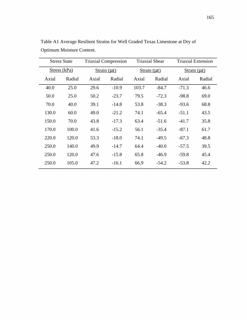
165
Table A1 Average Resilient Strains for Well Graded Texas Limestone at Dry of
Optimum Moisture Content.
Stress State Triaxial Compression Triaxial Shear Triaxial Extension
Stress (kPa) Strain (µε) Strain (µε) Strain (µε)
Axial Radial Axial Radial Axial Radial Axial Radial
40.0 25.0 29.6 -10.9 103.7 -84.7 -71.3 46.6
50.0 25.0 50.2 -23.7 79.5 -72.3 -98.8 69.0
70.0 40.0 39.1 -14.8 53.8 -38.3 -93.6 68.8
130.0 60.0 49.0 -21.2 74.1 -65.4 -51.1 43.5
150.0 70.0 43.8 -17.3 63.4 -51.6 -41.7 35.8
170.0 100.0 41.6 -15.2 56.1 -35.4 -87.1 61.7
220.0 120.0 53.3 -18.0 74.1 -49.5 -67.3 48.8
250.0 140.0 49.9 -14.7 64.4 -40.0 -57.5 39.5
250.0 120.0 47.6 -15.8 65.8 -46.9 -59.8 45.4
250.0 105.0 47.2 -16.1 66.9 -54.2 -53.8 42.2
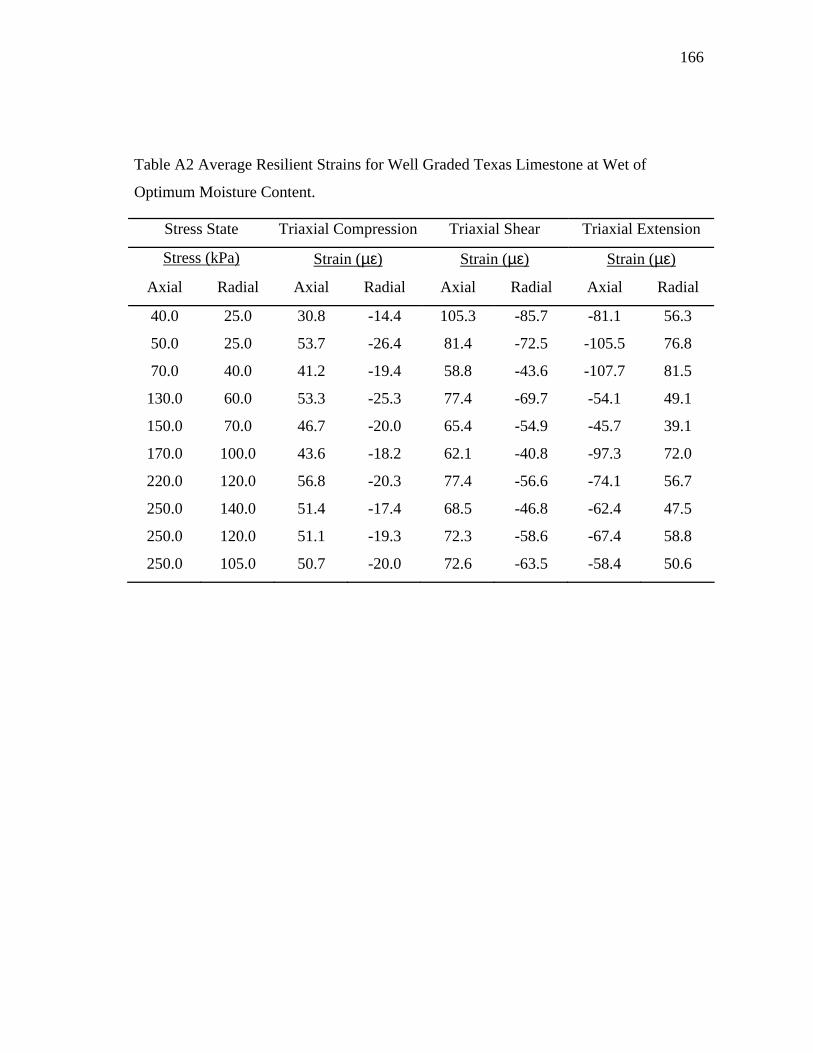
166
Table A2 Average Resilient Strains for Well Graded Texas Limestone at Wet of
Optimum Moisture Content.
Stress State Triaxial Compression Triaxial Shear Triaxial Extension
Stress (kPa) Strain (µε) Strain (µε) Strain (µε)
Axial Radial Axial Radial Axial Radial Axial Radial
40.0 25.0 30.8 -14.4 105.3 -85.7 -81.1 56.3
50.0 25.0 53.7 -26.4 81.4 -72.5 -105.5 76.8
70.0 40.0 41.2 -19.4 58.8 -43.6 -107.7 81.5
130.0 60.0 53.3 -25.3 77.4 -69.7 -54.1 49.1
150.0 70.0 46.7 -20.0 65.4 -54.9 -45.7 39.1
170.0 100.0 43.6 -18.2 62.1 -40.8 -97.3 72.0
220.0 120.0 56.8 -20.3 77.4 -56.6 -74.1 56.7
250.0 140.0 51.4 -17.4 68.5 -46.8 -62.4 47.5
250.0 120.0 51.1 -19.3 72.3 -58.6 -67.4 58.8
250.0 105.0 50.7 -20.0 72.6 -63.5 -58.4 50.6

167
Table A3 Average Resilient Strains for Fine Graded Texas Limestone at Optimum
Moisture Content.
Stress State Triaxial Compression Triaxial Shear Triaxial Extension
Stress (kPa) Strain (µε) Strain (µε) Strain (µε)
Axial Radial Axial Radial Axial Radial Axial Radial
40.0 25.0 36.7 -24.6 137.7 -163.3 -123.2 119.6
50.0 25.0 57.1 -36.9 93.1 -111.4 -133.6 126.0
70.0 40.0 44.1 -24.3 67.6 -65.5 -150.6 143.1
130.0 60.0 54.1 -30.6 88.4 -103.0 -64.1 70.3
150.0 70.0 48.0 -24.2 75.2 -79.7 -53.4 55.8
170.0 100.0 45.6 -21.2 66.5 -54.6 -120.1 104.7
220.0 120.0 57.3 -25.6 85.1 -75.4 -83.8 75.7
250.0 140.0 53.3 -20.6 74.5 -59.7 -70.5 59.7
250.0 120.0 50.6 -22.4 75.6 -74.0 -73.3 73.6
250.0 105.0 48.8 -23.1 74.8 -84.0 -63.2 65.1
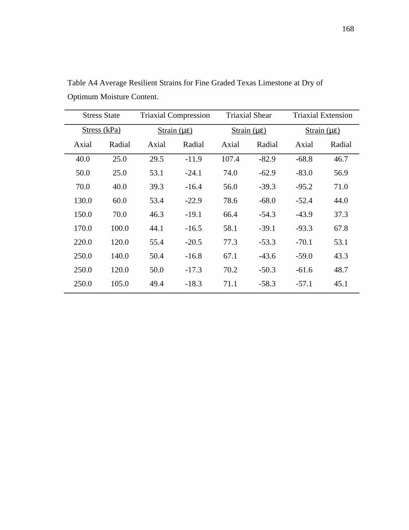
168
Table A4 Average Resilient Strains for Fine Graded Texas Limestone at Dry of
Optimum Moisture Content.
Stress State Triaxial Compression Triaxial Shear Triaxial Extension
Stress (kPa) Strain (µε) Strain (µε) Strain (µε)
Axial Radial Axial Radial Axial Radial Axial Radial
40.0 25.0 29.5 -11.9 107.4 -82.9 -68.8 46.7
50.0 25.0 53.1 -24.1 74.0 -62.9 -83.0 56.9
70.0 40.0 39.3 -16.4 56.0 -39.3 -95.2 71.0
130.0 60.0 53.4 -22.9 78.6 -68.0 -52.4 44.0
150.0 70.0 46.3 -19.1 66.4 -54.3 -43.9 37.3
170.0 100.0 44.1 -16.5 58.1 -39.1 -93.3 67.8
220.0 120.0 55.4 -20.5 77.3 -53.3 -70.1 53.1
250.0 140.0 50.4 -16.8 67.1 -43.6 -59.0 43.3
250.0 120.0 50.0 -17.3 70.2 -50.3 -61.6 48.7
250.0 105.0 49.4 -18.3 71.1 -58.3 -57.1 45.1

169
Table A5 Average Resilient Strains for Fine Graded Texas Limestone at Wet of
Optimum Moisture Content.
Stress State Triaxial Compression Triaxial Shear Triaxial Extension
Stress (kPa) Strain (µε) Strain (µε) Strain (µε)
Axial Radial Axial Radial Axial Radial Axial Radial
40.0 25.0 58.1 -53.6 226.4 -343.1 -479.5 545.4
50.0 25.0 69.9 -60.8 121.1 -190.1 -249.9 291.7
70.0 40.0 52.6 -37.3 88.4 -105.6 -279.0 295.6
130.0 60.0 58.0 -37.9 98.8 -137.3 -80.5 98.6
150.0 70.0 49.5 -29.4 81.8 -105.3 -64.1 77.2
170.0 100.0 50.3 -27.1 76.6 -73.3 -165.7 155.7
220.0 120.0 59.9 -30.8 94.8 -97.7 -105.8 103.3
250.0 140.0 55.2 -24.6 80.8 -75.5 -85.4 78.0
250.0 120.0 51.8 -25.2 79.0 -87.4 -82.9 89.8
250.0 105.0 47.5 -25.3 75.5 -94.6 -65.6 73.6

170
Table A6 Average Resilient Strains for Coarse Graded Texas Limestone at Optimum
Moisture Content.
Stress State Triaxial Compression Triaxial Shear Triaxial Extension
Stress (kPa) Strain (µε) Strain (µε) Strain (µε)
Axial Radial Axial Radial Axial Radial Axial Radial
40.0 25.0 34.9 -11.0 113.5 -84.1 -82.9 51.5
50.0 25.0 59.2 -24.1 87.7 -73.7 -109.7 69.2
70.0 40.0 44.1 -16.0 61.6 -42.3 -102.1 72.1
130.0 60.0 55.4 -21.4 78.8 -68.8 -54.0 48.3
150.0 70.0 49.4 -18.1 68.6 -56.6 -47.3 41.3
170.0 100.0 47.3 -15.2 61.2 -40.1 -92.0 67.9
220.0 120.0 60.4 -18.6 76.6 -55.0 -58.2 44.6
250.0 140.0 53.8 -16.7 71.6 -46.5 -63.2 48.4
250.0 120.0 53.5 -16.8 71.2 -53.8 -63.6 54.9
250.0 105.0 52.7 -17.8 71.8 -60.1 -58.4 48.8
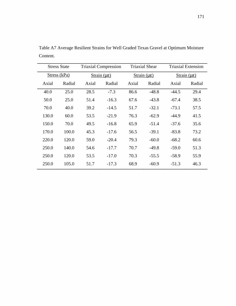
171
Table A7 Average Resilient Strains for Well Graded Texas Gravel at Optimum Moisture
Content.
Stress State Triaxial Compression Triaxial Shear Triaxial Extension
Stress (kPa) Strain (µε) Strain (µε) Strain (µε)
Axial Radial Axial Radial Axial Radial Axial Radial
40.0 25.0 28.5 -7.3 86.6 -48.8 -44.5 29.4
50.0 25.0 51.4 -16.3 67.6 -43.8 -67.4 38.5
70.0 40.0 39.2 -14.5 51.7 -32.1 -73.1 57.5
130.0 60.0 53.5 -21.9 76.3 -62.9 -44.9 41.5
150.0 70.0 49.5 -16.8 65.9 -51.4 -37.6 35.6
170.0 100.0 45.3 -17.6 56.5 -39.1 -83.8 73.2
220.0 120.0 59.0 -20.4 79.3 -60.0 -68.2 60.6
250.0 140.0 54.6 -17.7 70.7 -49.8 -59.0 51.3
250.0 120.0 53.5 -17.0 70.3 -55.5 -58.9 55.9
250.0 105.0 51.7 -17.3 68.9 -60.9 -51.3 46.3

172
Table A8 Average Resilient Strains for Well Graded Texas Gravel at Dry of Optimum
Moisture Content.
Stress State Triaxial Compression Triaxial Shear Triaxial Extension
Stress (kPa) Strain (µε) Strain (µε) Strain (µε)
Axial Radial Axial Radial Axial Radial Axial Radial
40.0 25.0 24.6 -3.8 60.7 -21.8 -34.5 13.1
50.0 25.0 39.8 -7.4 47.8 -19.4 -47.3 16.8
70.0 40.0 32.6 -6.0 37.0 -14.3 -47.4 23.6
130.0 60.0 45.7 -9.6 57.5 -28.5 -32.1 19.9
150.0 70.0 40.2 -9.0 52.2 -23.3 -28.6 17.9
170.0 100.0 38.6 -7.7 44.5 -19.4 -55.9 33.1
220.0 120.0 54.2 -9.0 63.8 -28.5 -53.5 29.5
250.0 140.0 48.5 -8.6 56.5 -25.6 -46.0 27.7
250.0 120.0 48.6 -7.6 57.1 -26.8 -44.2 28.7
250.0 105.0 48.3 -7.8 56.3 -28.4 -43.0 22.6
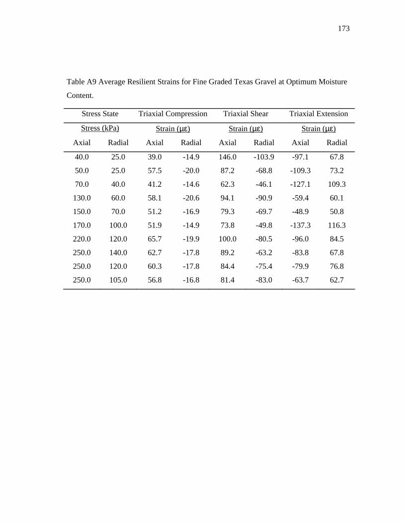
173
Table A9 Average Resilient Strains for Fine Graded Texas Gravel at Optimum Moisture
Content.
Stress State Triaxial Compression Triaxial Shear Triaxial Extension
Stress (kPa) Strain (µε) Strain (µε) Strain (µε)
Axial Radial Axial Radial Axial Radial Axial Radial
40.0 25.0 39.0 -14.9 146.0 -103.9 -97.1 67.8
50.0 25.0 57.5 -20.0 87.2 -68.8 -109.3 73.2
70.0 40.0 41.2 -14.6 62.3 -46.1 -127.1 109.3
130.0 60.0 58.1 -20.6 94.1 -90.9 -59.4 60.1
150.0 70.0 51.2 -16.9 79.3 -69.7 -48.9 50.8
170.0 100.0 51.9 -14.9 73.8 -49.8 -137.3 116.3
220.0 120.0 65.7 -19.9 100.0 -80.5 -96.0 84.5
250.0 140.0 62.7 -17.8 89.2 -63.2 -83.8 67.8
250.0 120.0 60.3 -17.8 84.4 -75.4 -79.9 76.8
250.0 105.0 56.8 -16.8 81.4 -83.0 -63.7 62.7
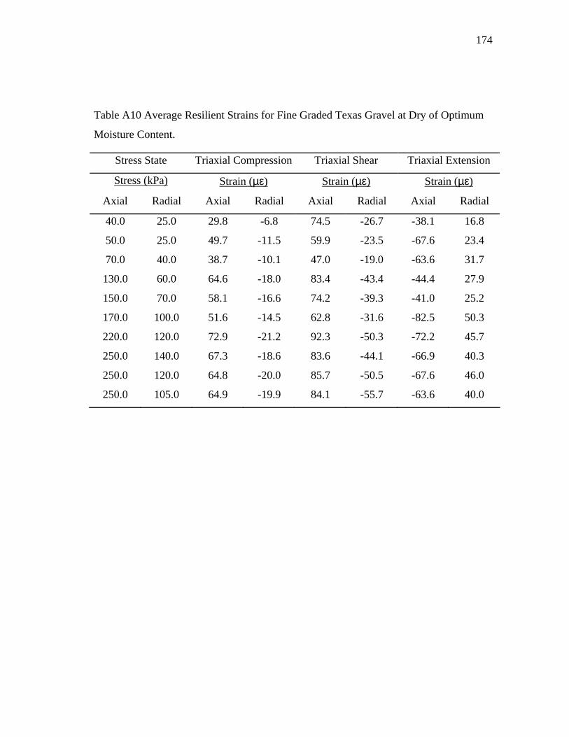
174
Table A10 Average Resilient Strains for Fine Graded Texas Gravel at Dry of Optimum
Moisture Content.
Stress State Triaxial Compression Triaxial Shear Triaxial Extension
Stress (kPa) Strain (µε) Strain (µε) Strain (µε)
Axial Radial Axial Radial Axial Radial Axial Radial
40.0 25.0 29.8 -6.8 74.5 -26.7 -38.1 16.8
50.0 25.0 49.7 -11.5 59.9 -23.5 -67.6 23.4
70.0 40.0 38.7 -10.1 47.0 -19.0 -63.6 31.7
130.0 60.0 64.6 -18.0 83.4 -43.4 -44.4 27.9
150.0 70.0 58.1 -16.6 74.2 -39.3 -41.0 25.2
170.0 100.0 51.6 -14.5 62.8 -31.6 -82.5 50.3
220.0 120.0 72.9 -21.2 92.3 -50.3 -72.2 45.7
250.0 140.0 67.3 -18.6 83.6 -44.1 -66.9 40.3
250.0 120.0 64.8 -20.0 85.7 -50.5 -67.6 46.0
250.0 105.0 64.9 -19.9 84.1 -55.7 -63.6 40.0

175
Table A11 Average Resilient Strains for Coarse Graded Texas Gravel at Optimum
Moisture Content.
Stress State Triaxial Compression Triaxial Shear Triaxial Extension
Stress (kPa) Strain (µε) Strain (µε) Strain (µε)
Axial Radial Axial Radial Axial Radial Axial Radial
40.0 25.0 31.8 -10.6 93.5 -60.0 -54.1 35.0
50.0 25.0 54.0 -17.2 71.1 -50.1 -77.0 45.8
70.0 40.0 42.6 -14.7 54.0 -36.5 -83.4 66.8
130.0 60.0 59.9 -25.6 86.8 -83.2 -55.9 56.8
150.0 70.0 52.7 -19.9 72.2 -63.7 -46.0 46.4
170.0 100.0 50.0 -20.1 65.6 -50.7 -103.4 93.3
220.0 120.0 64.2 -23.8 87.6 -70.8 -80.6 75.2
250.0 140.0 59.7 -20.8 79.5 -61.1 -70.5 63.9
250.0 120.0 58.7 -21.4 81.5 -68.8 -71.6 72.4
250.0 105.0 56.9 -20.5 79.6 -69.2 -59.7 57.5

176
Table A12 Average Resilient Strains for Well Graded Minnesota Gravel at Optimum
Moisture Content.
Stress State Triaxial Compression Triaxial Shear Triaxial Extension
Stress (kPa) Strain (µε) Strain (µε) Strain (µε)
Axial Radial Axial Radial Axial Radial Axial Radial
40.0 25.0 42.3 -18.2 131.6 -121.9 -98.4 80.7
50.0 25.0 68.5 -37.9 111.7 -121.4 -140.7 121.2
70.0 40.0 49.2 -23.7 75.2 -67.9 -136.0 122.1
130.0 60.0 70.5 -36.5 114.1 -120.5 -76.3 80.3
150.0 70.0 64.6 -29.7 96.8 -95.7 -62.3 66.7
170.0 100.0 61.8 -25.9 84.5 -66.6 -128.7 112.5
220.0 120.0 79.1 -31.6 113.4 -92.3 -103.1 90.9
250.0 140.0 71.3 -27.1 98.0 -75.9 -85.8 75.3
250.0 120.0 68.8 -29.4 99.8 -93.3 -88.8 91.8
250.0 105.0 67.9 -32.0 101.7 -108.9 -81.2 84.1
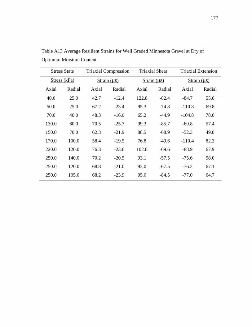
177
Table A13 Average Resilient Strains for Well Graded Minnesota Gravel at Dry of
Optimum Moisture Content.
Stress State Triaxial Compression Triaxial Shear Triaxial Extension
Stress (kPa) Strain (µε) Strain (µε) Strain (µε)
Axial Radial Axial Radial Axial Radial Axial Radial
40.0 25.0 42.7 -12.4 122.8 -82.4 -84.7 55.0
50.0 25.0 67.2 -23.4 95.3 -74.8 -110.8 69.8
70.0 40.0 48.3 -16.0 65.2 -44.9 -104.8 78.0
130.0 60.0 70.5 -25.7 99.3 -85.7 -60.8 57.4
150.0 70.0 62.3 -21.9 88.5 -68.9 -52.3 49.0
170.0 100.0 58.4 -19.5 76.8 -49.6 -110.4 82.3
220.0 120.0 76.3 -23.6 102.8 -69.6 -88.9 67.9
250.0 140.0 70.2 -20.5 93.1 -57.5 -75.6 58.0
250.0 120.0 68.8 -21.0 93.0 -67.5 -76.2 67.1
250.0 105.0 68.2 -23.9 95.0 -84.5 -77.0 64.7
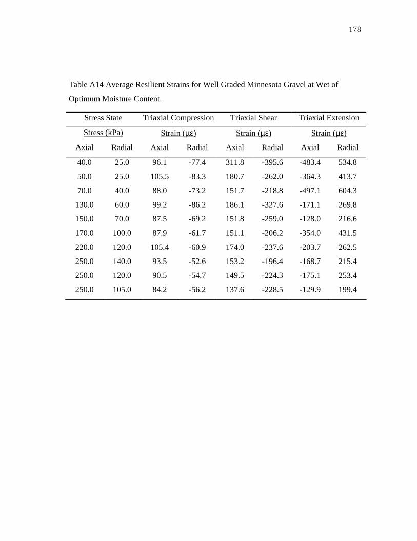
178
Table A14 Average Resilient Strains for Well Graded Minnesota Gravel at Wet of
Optimum Moisture Content.
Stress State Triaxial Compression Triaxial Shear Triaxial Extension
Stress (kPa) Strain (µε) Strain (µε) Strain (µε)
Axial Radial Axial Radial Axial Radial Axial Radial
40.0 25.0 96.1 -77.4 311.8 -395.6 -483.4 534.8
50.0 25.0 105.5 -83.3 180.7 -262.0 -364.3 413.7
70.0 40.0 88.0 -73.2 151.7 -218.8 -497.1 604.3
130.0 60.0 99.2 -86.2 186.1 -327.6 -171.1 269.8
150.0 70.0 87.5 -69.2 151.8 -259.0 -128.0 216.6
170.0 100.0 87.9 -61.7 151.1 -206.2 -354.0 431.5
220.0 120.0 105.4 -60.9 174.0 -237.6 -203.7 262.5
250.0 140.0 93.5 -52.6 153.2 -196.4 -168.7 215.4
250.0 120.0 90.5 -54.7 149.5 -224.3 -175.1 253.4
250.0 105.0 84.2 -56.2 137.6 -228.5 -129.9 199.4
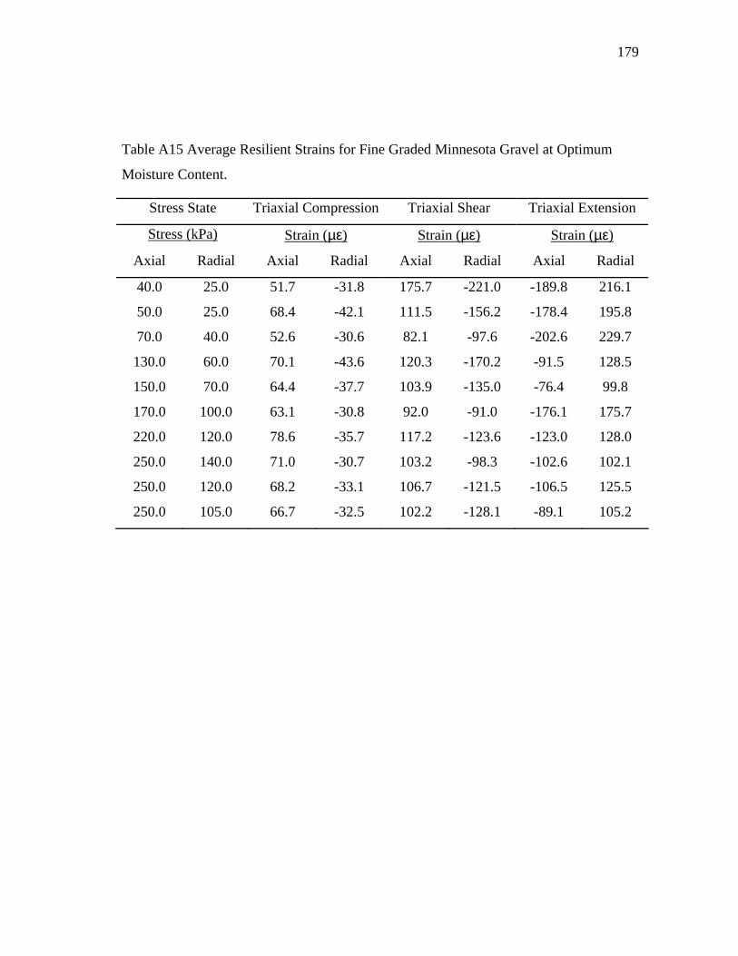
179
Table A15 Average Resilient Strains for Fine Graded Minnesota Gravel at Optimum
Moisture Content.
Stress State Triaxial Compression Triaxial Shear Triaxial Extension
Stress (kPa) Strain (µε) Strain (µε) Strain (µε)
Axial Radial Axial Radial Axial Radial Axial Radial
40.0 25.0 51.7 -31.8 175.7 -221.0 -189.8 216.1
50.0 25.0 68.4 -42.1 111.5 -156.2 -178.4 195.8
70.0 40.0 52.6 -30.6 82.1 -97.6 -202.6 229.7
130.0 60.0 70.1 -43.6 120.3 -170.2 -91.5 128.5
150.0 70.0 64.4 -37.7 103.9 -135.0 -76.4 99.8
170.0 100.0 63.1 -30.8 92.0 -91.0 -176.1 175.7
220.0 120.0 78.6 -35.7 117.2 -123.6 -123.0 128.0
250.0 140.0 71.0 -30.7 103.2 -98.3 -102.6 102.1
250.0 120.0 68.2 -33.1 106.7 -121.5 -106.5 125.5
250.0 105.0 66.7 -32.5 102.2 -128.1 -89.1 105.2
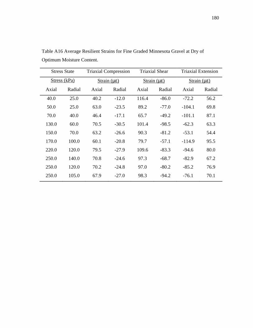
180
Table A16 Average Resilient Strains for Fine Graded Minnesota Gravel at Dry of
Optimum Moisture Content.
Stress State Triaxial Compression Triaxial Shear Triaxial Extension
Stress (kPa) Strain (µε) Strain (µε) Strain (µε)
Axial Radial Axial Radial Axial Radial Axial Radial
40.0 25.0 40.2 -12.0 116.4 -86.0 -72.2 56.2
50.0 25.0 63.0 -23.5 89.2 -77.0 -104.1 69.8
70.0 40.0 46.4 -17.1 65.7 -49.2 -101.1 87.1
130.0 60.0 70.5 -30.5 101.4 -98.5 -62.3 63.3
150.0 70.0 63.2 -26.6 90.3 -81.2 -53.1 54.4
170.0 100.0 60.1 -20.8 79.7 -57.1 -114.9 95.5
220.0 120.0 79.5 -27.9 109.6 -83.3 -94.6 80.0
250.0 140.0 70.8 -24.6 97.3 -68.7 -82.9 67.2
250.0 120.0 70.2 -24.8 97.0 -80.2 -85.2 76.9
250.0 105.0 67.9 -27.0 98.3 -94.2 -76.1 70.1

181
Table A17 Average Resilient Strains for Well Graded California Granite at Optimum
Moisture Content.
Stress State Triaxial Compression Triaxial Shear Triaxial Extension
Stress (kPa) Strain (µε) Strain (µε) Strain (µε)
Axial Radial Axial Radial Axial Radial Axial Radial
40.0 25.0 47.1 -18.8 148.0 -130.4 -97.4 76.6
50.0 25.0 70.4 -32.9 107.9 -112.2 -141.3 110.1
70.0 40.0 49.7 -19.9 73.7 -62.6 -131.6 111.7
130.0 60.0 76.0 -35.9 113.2 -120.8 -76.3 82.2
150.0 70.0 67.5 -31.3 98.6 -97.3 -65.7 68.4
170.0 100.0 63.0 -23.9 88.0 -68.7 -134.7 111.9
220.0 120.0 79.7 -30.7 113.5 -92.8 -103.6 90.0
250.0 140.0 72.1 -24.8 101.3 -75.7 -90.9 75.6
250.0 120.0 73.0 -26.7 102.7 -88.3 -91.7 88.6
250.0 105.0 69.6 -29.7 103.5 -103.5 -84.1 81.8

182
Table A18 Average Resilient Strains for Well Graded California Granite at Dry of
Optimum Moisture Content.
Stress State Triaxial Compression Triaxial Shear Triaxial Extension
Stress (kPa) Strain (µε) Strain (µε) Strain (µε)
Axial Radial Axial Radial Axial Radial Axial Radial
40.0 25.0 40.4 -11.0 118.8 -84.4 -90.2 61.1
50.0 25.0 62.5 -20.9 90.2 -77.5 -120.5 77.9
70.0 40.0 46.8 -15.0 64.5 -47.0 -116.3 92.5
130.0 60.0 66.7 -24.1 99.8 -96.8 -65.8 66.2
150.0 70.0 62.0 -25.4 88.5 -77.4 -54.8 58.7
170.0 100.0 56.0 -18.2 74.4 -54.7 -112.9 96.5
220.0 120.0 73.5 -23.0 100.5 -77.9 -90.6 78.6
250.0 140.0 67.5 -19.4 89.8 -64.9 -78.2 67.7
250.0 120.0 64.5 -21.4 91.0 -77.8 -79.5 79.5
250.0 105.0 66.3 -25.2 91.6 -87.9 -72.9 70.7

183
Table A19 Average Resilient Strains for Well Graded California Granite at Wet of
Optimum Moisture Content.
Stress State Triaxial Compression Triaxial Shear Triaxial Extension
Stress (kPa) Strain (µε) Strain (µε) Strain (µε)
Axial Radial Axial Radial Axial Radial Axial Radial
40.0 25.0 42.0 -16.2 140.4 -124.8 -108.5 82.8
50.0 25.0 67.8 -33.2 111.3 -117.5 -155.8 124.0
70.0 40.0 52.2 -21.7 76.0 -64.1 -142.5 123.2
130.0 60.0 70.1 -32.9 109.5 -111.9 -74.0 76.5
150.0 70.0 62.1 -25.7 92.7 -91.3 -62.0 64.9
170.0 100.0 60.5 -20.9 82.2 -61.6 -127.9 106.7
220.0 120.0 75.2 -27.3 108.2 -87.2 -98.7 85.9
250.0 140.0 69.4 -23.5 93.7 -71.8 -83.4 72.6
250.0 120.0 68.0 -25.2 100.8 -88.2 -88.7 85.8
250.0 105.0 66.2 -28.3 97.6 -97.6 -77.5 76.2
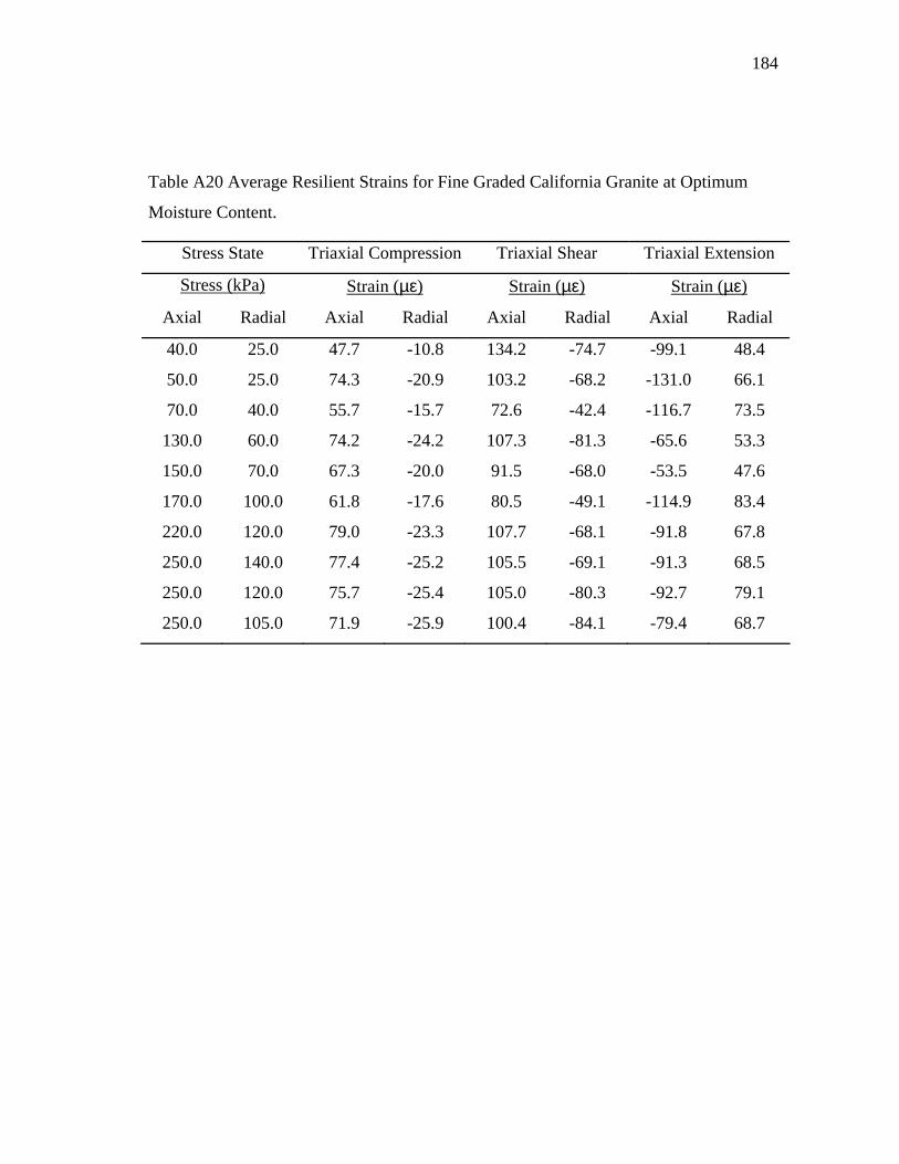
184
Table A20 Average Resilient Strains for Fine Graded California Granite at Optimum
Moisture Content.
Stress State Triaxial Compression Triaxial Shear Triaxial Extension
Stress (kPa) Strain (µε) Strain (µε) Strain (µε)
Axial Radial Axial Radial Axial Radial Axial Radial
40.0 25.0 47.7 -10.8 134.2 -74.7 -99.1 48.4
50.0 25.0 74.3 -20.9 103.2 -68.2 -131.0 66.1
70.0 40.0 55.7 -15.7 72.6 -42.4 -116.7 73.5
130.0 60.0 74.2 -24.2 107.3 -81.3 -65.6 53.3
150.0 70.0 67.3 -20.0 91.5 -68.0 -53.5 47.6
170.0 100.0 61.8 -17.6 80.5 -49.1 -114.9 83.4
220.0 120.0 79.0 -23.3 107.7 -68.1 -91.8 67.8
250.0 140.0 77.4 -25.2 105.5 -69.1 -91.3 68.5
250.0 120.0 75.7 -25.4 105.0 -80.3 -92.7 79.1
250.0 105.0 71.9 -25.9 100.4 -84.1 -79.4 68.7

185
Table A21 Average Resilient Strains for Fine Graded California Granite at Dry of
Optimum Moisture Content.
Stress State Triaxial Compression Triaxial Shear Triaxial Extension
Stress (kPa) Strain (µε) Strain (µε) Strain (µε)
Axial Radial Axial Radial Axial Radial Axial Radial
40.0 25.0 33.6 -9.2 93.8 -62.1 -61.7 43.0
50.0 25.0 54.7 -15.1 72.4 -55.6 -91.4 53.9
70.0 40.0 42.9 -11.9 55.7 -36.9 -91.4 68.4
130.0 60.0 62.2 -21.7 87.8 -71.7 -52.2 50.7
150.0 70.0 55.1 -18.6 77.7 -59.8 -45.3 42.5
170.0 100.0 53.2 -15.4 66.7 -45.7 -98.8 80.5
220.0 120.0 68.2 -20.5 93.2 -64.4 -78.3 64.3
250.0 140.0 62.2 -17.6 81.8 -54.1 -70.1 54.8
250.0 120.0 63.0 -18.6 84.7 -66.0 -71.6 64.3
250.0 105.0 61.8 -22.0 83.7 -75.2 -65.4 59.7
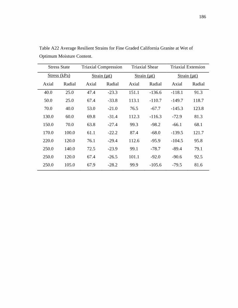
186
Table A22 Average Resilient Strains for Fine Graded California Granite at Wet of
Optimum Moisture Content.
Stress State Triaxial Compression Triaxial Shear Triaxial Extension
Stress (kPa) Strain (µε) Strain (µε) Strain (µε)
Axial Radial Axial Radial Axial Radial Axial Radial
40.0 25.0 47.4 -23.3 151.1 -136.6 -118.1 91.3
50.0 25.0 67.4 -33.8 113.1 -110.7 -149.7 118.7
70.0 40.0 53.0 -21.0 76.5 -67.7 -145.3 123.8
130.0 60.0 69.8 -31.4 112.3 -116.3 -72.9 81.3
150.0 70.0 63.8 -27.4 99.3 -98.2 -66.1 68.1
170.0 100.0 61.1 -22.2 87.4 -68.0 -139.5 121.7
220.0 120.0 76.1 -29.4 112.6 -95.9 -104.5 95.8
250.0 140.0 72.5 -23.9 99.1 -78.7 -89.4 79.1
250.0 120.0 67.4 -26.5 101.1 -92.0 -90.6 92.5
250.0 105.0 67.9 -28.2 99.9 -105.6 -79.5 81.6
187
APPENDIX B
TABLES OF MODULI AND POISSON’S RATIO
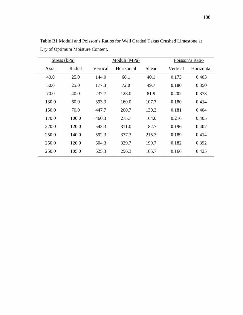
188
Table B1 Moduli and Poisson’s Ratios for Well Graded Texas Crushed Limestone at
Dry of Optimum Moisture Content.
Stress (kPa) Moduli (MPa) Poisson’s Ratio
Axial Radial Vertical Horizontal Shear Vertical Horizontal
40.0 25.0 144.0 68.1 40.1 0.173 0.403
50.0 25.0 177.3 72.0 49.7 0.180 0.350
70.0 40.0 237.7 128.0 81.9 0.202 0.373
130.0 60.0 393.3 160.0 107.7 0.180 0.414
150.0 70.0 447.7 200.7 130.3 0.181 0.404
170.0 100.0 460.3 275.7 164.0 0.216 0.405
220.0 120.0 543.3 311.0 182.7 0.196 0.407
250.0 140.0 592.3 377.3 215.3 0.189 0.414
250.0 120.0 604.3 329.7 199.7 0.182 0.392
250.0 105.0 625.3 296.3 185.7 0.166 0.425
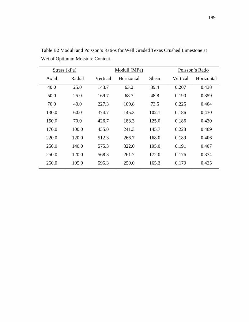
189
Table B2 Moduli and Poisson’s Ratios for Well Graded Texas Crushed Limestone at
Wet of Optimum Moisture Content.
Stress (kPa) Moduli (MPa) Poisson’s Ratio
Axial Radial Vertical Horizontal Shear Vertical Horizontal
40.0 25.0 143.7 63.2 39.4 0.207 0.438
50.0 25.0 169.7 68.7 48.8 0.190 0.359
70.0 40.0 227.3 109.8 73.5 0.225 0.404
130.0 60.0 374.7 145.3 102.1 0.186 0.430
150.0 70.0 426.7 183.3 125.0 0.186 0.430
170.0 100.0 435.0 241.3 145.7 0.228 0.409
220.0 120.0 512.3 266.7 168.0 0.189 0.406
250.0 140.0 575.3 322.0 195.0 0.191 0.407
250.0 120.0 568.3 261.7 172.0 0.176 0.374
250.0 105.0 595.3 250.0 165.3 0.170 0.435

190
Table B3 Moduli and Poisson’s Ratios for Fine Graded Texas Crushed Limestone at
Optimum Moisture Content.
Stress (kPa) Moduli (MPa) Poisson’s Ratio
Axial Radial Vertical Horizontal Shear Vertical Horizontal
40.0 25.0 124.0 33.6 25.3 0.185 0.402
50.0 25.0 156.3 44.5 36.9 0.175 0.325
70.0 40.0 203.3 72.8 56.8 0.202 0.319
130.0 60.0 360.0 102.2 78.7 0.166 0.390
150.0 70.0 404.3 131.3 97.0 0.167 0.384
170.0 100.0 407.7 179.0 124.0 0.203 0.354
220.0 120.0 503.7 204.7 140.7 0.183 0.392
250.0 140.0 549.7 256.3 168.0 0.182 0.394
250.0 120.0 571.7 210.0 151.0 0.166 0.362
250.0 105.0 211.3 232.3 142.3 0.152 0.412

191
Table B4 Moduli and Poisson’s Ratios for Fine Graded Texas Crushed Limestone at Dry
of Optimum Moisture Content.
Stress (kPa) Moduli (MPa) Poisson’s Ratio
Axial Radial Vertical Horizontal Shear Vertical Horizontal
40.0 25.0 145.7 69.8 39.4 0.191 0.421
50.0 25.0 189.3 75.5 55.6 0.182 0.455
70.0 40.0 237.0 124.3 78.7 0.218 0.390
130.0 60.0 368.7 153.0 102.3 0.182 0.434
150.0 70.0 428.0 189.3 124.3 0.186 0.425
170.0 100.0 437.3 245.7 154.7 0.208 0.411
220.0 120.0 531.0 284.3 172.3 0.202 0.420
250.0 140.0 589.7 345.7 203.3 0.198 0.424
250.0 120.0 581.7 307.7 187.0 0.186 0.395
250.0 105.0 602.3 274.0 174.0 0.174 0.442
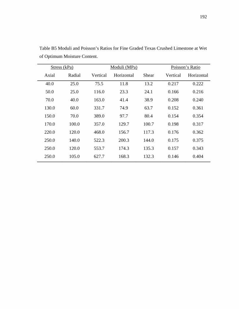
192
Table B5 Moduli and Poisson’s Ratios for Fine Graded Texas Crushed Limestone at Wet
of Optimum Moisture Content.
Stress (kPa) Moduli (MPa) Poisson’s Ratio
Axial Radial Vertical Horizontal Shear Vertical Horizontal
40.0 25.0 75.5 11.8 13.2 0.217 0.222
50.0 25.0 116.0 23.3 24.1 0.166 0.216
70.0 40.0 163.0 41.4 38.9 0.208 0.240
130.0 60.0 331.7 74.9 63.7 0.152 0.361
150.0 70.0 389.0 97.7 80.4 0.154 0.354
170.0 100.0 357.0 129.7 100.7 0.198 0.317
220.0 120.0 468.0 156.7 117.3 0.176 0.362
250.0 140.0 522.3 200.3 144.0 0.175 0.375
250.0 120.0 553.7 174.3 135.3 0.157 0.343
250.0 105.0 627.7 168.3 132.3 0.146 0.404

193
Table B6 Moduli and Poisson’s Ratios for Coarse Graded Texas Crushed Limestone at
Optimum Moisture Content.
Stress (kPa) Moduli (MPa) Poisson’s Ratio
Axial Radial Vertical Horizontal Shear Vertical Horizontal
40.0 25.0 119.3 67.7 38.1 0.171 0.369
50.0 25.0 151.3 70.1 46.6 0.177 0.355
70.0 40.0 208.0 117.7 72.3 0.203 0.380
130.0 60.0 351.0 149.7 101.8 0.167 0.384
150.0 70.0 394.0 180.7 120.0 0.169 0.380
170.0 100.0 407.0 244.7 148.3 0.190 0.381
220.0 120.0 526.0 281.0 171.3 0.173 0.467
250.0 140.0 543.7 327.0 190.7 0.187 0.382
250.0 120.0 547.7 283.7 180.3 0.164 0.355
250.0 105.0 570.0 262.7 171.0 0.160 0.415
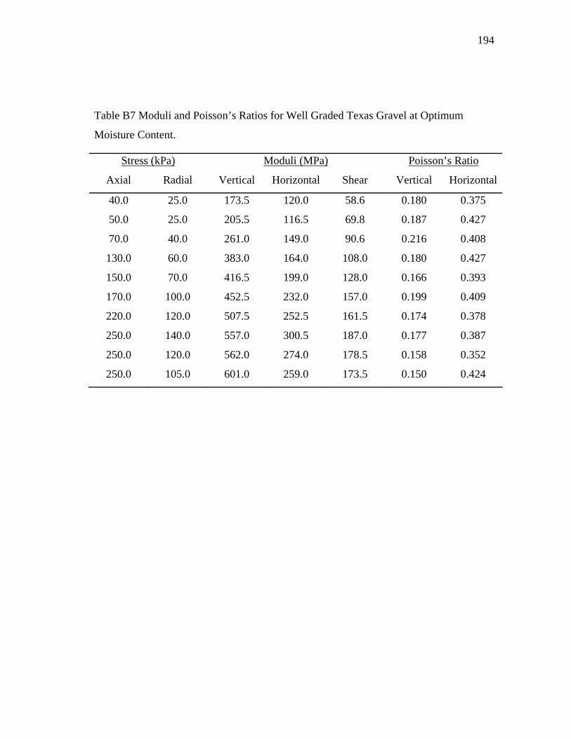
194
Table B7 Moduli and Poisson’s Ratios for Well Graded Texas Gravel at Optimum
Moisture Content.
Stress (kPa) Moduli (MPa) Poisson’s Ratio
Axial Radial Vertical Horizontal Shear Vertical Horizontal
40.0 25.0 173.5 120.0 58.6 0.180 0.375
50.0 25.0 205.5 116.5 69.8 0.187 0.427
70.0 40.0 261.0 149.0 90.6 0.216 0.408
130.0 60.0 383.0 164.0 108.0 0.180 0.427
150.0 70.0 416.5 199.0 128.0 0.166 0.393
170.0 100.0 452.5 232.0 157.0 0.199 0.409
220.0 120.0 507.5 252.5 161.5 0.174 0.378
250.0 140.0 557.0 300.5 187.0 0.177 0.387
250.0 120.0 562.0 274.0 178.5 0.158 0.352
250.0 105.0 601.0 259.0 173.5 0.150 0.424

195
Table B8 Moduli and Poisson’s Ratios for Well Graded Texas Gravel at Dry of
Optimum Moisture Content.
Stress (kPa) Moduli (MPa) Poisson’s Ratio
Axial Radial Vertical Horizontal Shear Vertical Horizontal
40.0 25.0 195.0 250.0 90.9 0.200 0.453
50.0 25.0 250.0 264.0 112.0 0.198 0.429
70.0 40.0 305.0 333.0 146.0 0.199 0.425
130.0 60.0 434.0 368.0 174.0 0.180 0.392
150.0 70.0 489.0 450.0 199.0 0.204 0.382
170.0 100.0 519.0 493.0 235.0 0.188 0.389
220.0 120.0 537.0 533.0 244.0 0.165 0.348
250.0 140.0 612.0 583.0 274.0 0.167 0.351
250.0 120.0 607.0 572.0 268.0 0.148 0.304
250.0 105.0 621.0 555.0 266.0 0.148 0.406

196
Table B9 Moduli and Poisson’s Ratios for Well Graded Texas Gravel at Wet of
Optimum Moisture Content.
Stress (kPa) Moduli (MPa) Poisson’s Ratio
Axial Radial Vertical Horizontal Shear Vertical Horizontal
40.0 25.0 48.2 25.6 14.3 0.160 0.212
50.0 25.0 88.1 36.1 26.1 0.140 0.250
70.0 40.0 106.0 50.5 36.9 0.145 0.109
130.0 60.0 240.0 82.9 59.7 0.138 0.362
150.0 70.0 261.0 135.0 83.1 0.125 0.250
170.0 100.0 238.0 121.0 85.4 0.155 0.132
220.0 120.0 294.0 198.0 115.0 0.162 0.169
250.0 140.0 318.0 298.0 142.0 0.152 0.053
250.0 120.0 376.0 464.0 188.0 0.152 0.174
250.0 105.0 470.0 546.0 238.0 0.118 0.406

197
Table B10 Moduli and Poisson’s Ratios for Fine Graded Texas Gravel at Optimum
Moisture Content.
Stress (kPa) Moduli (MPa) Poisson’s Ratio
Axial Radial Vertical Horizontal Shear Vertical Horizontal
40.0 25.0 104.0 56.1 30.0 0.193 0.348
50.0 25.0 147.0 76.6 48.1 0.162 0.236
70.0 40.0 192.0 107.0 69.2 0.180 0.168
130.0 60.0 308.0 123.0 81.1 0.137 0.299
150.0 70.0 356.0 157.0 101.0 0.141 0.278
170.0 100.0 310.0 199.0 121.0 0.165 0.147
220.0 120.0 393.0 202.0 125.0 0.147 0.259
250.0 140.0 428.0 251.0 148.0 0.159 0.289
250.0 120.0 455.0 210.0 141.0 0.134 0.280
250.0 105.0 504.0 201.0 137.0 0.119 0.332

198
Table B11 Moduli and Poisson’s Ratios for Fine Graded Texas Gravel at Dry of
Optimum Moisture Content.
Stress (kPa) Moduli (MPa) Poisson’s Ratio
Axial Radial Vertical Horizontal Shear Vertical Horizontal
40.0 25.0 172.0 192.0 74.1 0.266 0.571
50.0 25.0 196.0 208.0 90.0 0.239 0.502
70.0 40.0 255.0 253.0 114.0 0.251 0.487
130.0 60.0 319.0 238.0 118.0 0.213 0.486
150.0 70.0 356.0 260.0 132.0 0.215 0.501
170.0 100.0 392.0 304.0 159.0 0.219 0.463
220.0 120.0 422.0 300.0 158.0 0.212 0.483
250.0 140.0 457.0 340.0 176.0 0.211 0.485
250.0 120.0 466.0 304.0 165.0 0.205 0.455
250.0 105.0 478.0 281.0 161.0 0.190 0.513
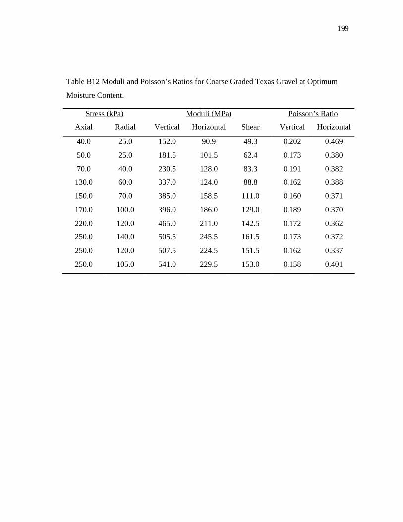
199
Table B12 Moduli and Poisson’s Ratios for Coarse Graded Texas Gravel at Optimum
Moisture Content.
Stress (kPa) Moduli (MPa) Poisson’s Ratio
Axial Radial Vertical Horizontal Shear Vertical Horizontal
40.0 25.0 152.0 90.9 49.3 0.202 0.469
50.0 25.0 181.5 101.5 62.4 0.173 0.380
70.0 40.0 230.5 128.0 83.3 0.191 0.382
130.0 60.0 337.0 124.0 88.8 0.162 0.388
150.0 70.0 385.0 158.5 111.0 0.160 0.371
170.0 100.0 396.0 186.0 129.0 0.189 0.370
220.0 120.0 465.0 211.0 142.5 0.172 0.362
250.0 140.0 505.5 245.5 161.5 0.173 0.372
250.0 120.0 507.5 224.5 151.5 0.162 0.337
250.0 105.0 541.0 229.5 153.0 0.158 0.401
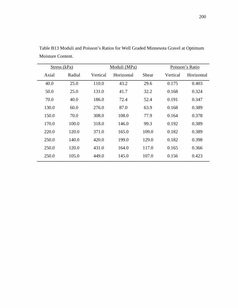
200
Table B13 Moduli and Poisson’s Ratios for Well Graded Minnesota Gravel at Optimum
Moisture Content.
Stress (kPa) Moduli (MPa) Poisson’s Ratio
Axial Radial Vertical Horizontal Shear Vertical Horizontal
40.0 25.0 110.0 43.2 29.6 0.175 0.403
50.0 25.0 131.0 41.7 32.2 0.168 0.324
70.0 40.0 186.0 72.4 52.4 0.191 0.347
130.0 60.0 276.0 87.0 63.9 0.168 0.389
150.0 70.0 308.0 108.0 77.9 0.164 0.378
170.0 100.0 318.0 146.0 99.3 0.192 0.389
220.0 120.0 371.0 165.0 109.0 0.182 0.389
250.0 140.0 420.0 199.0 129.0 0.182 0.398
250.0 120.0 431.0 164.0 117.0 0.165 0.366
250.0 105.0 449.0 145.0 107.0 0.156 0.423

201
Table B14 Moduli and Poisson’s Ratios for Well Graded Minnesota Gravel at Dry of
Optimum Moisture Content.
Stress (kPa) Moduli (MPa) Poisson’s Ratio
Axial Radial Vertical Horizontal Shear Vertical Horizontal
40.0 25.0 106.0 65.4 36.6 0.178 0.385
50.0 25.0 137.0 69.1 44.1 0.168 0.336
70.0 40.0 192.0 110.0 68.2 0.188 0.354
130.0 60.0 282.0 122.0 81.1 0.160 0.380
150.0 70.0 318.0 151.0 95.3 0.170 0.371
170.0 100.0 333.0 198.0 119.0 0.198 0.394
220.0 120.0 383.0 221.0 131.0 0.180 0.388
250.0 140.0 422.0 267.0 149.0 0.186 0.386
250.0 120.0 428.0 229.0 140.0 0.165 0.354
250.0 105.0 438.0 189.0 125.0 0.155 0.420

202
Table B15 Moduli and Poisson’s Ratios for Well Graded Minnesota Gravel at Wet of
Optimum Moisture Content.
Stress (kPa) Moduli (MPa) Poisson’s Ratio
Axial Radial Vertical Horizontal Shear Vertical Horizontal
40.0 25.0 47.3 10.6 10.6 0.209 0.281
50.0 25.0 75.3 17.1 16.9 0.166 0.186
70.0 40.0 102.0 19.3 20.2 0.193 0.242
130.0 60.0 195.0 30.2 29.2 0.142 0.314
150.0 70.0 226.0 37.9 36.5 0.136 0.303
170.0 100.0 206.0 45.6 42.0 0.170 0.282
220.0 120.0 268.0 63.4 54.7 0.145 0.299
250.0 140.0 304.0 77.0 64.4 0.149 0.305
250.0 120.0 312.0 66.7 60.2 0.135 0.281
250.0 105.0 361.0 67.3 61.5 0.127 0.358

203
Table B16 Moduli and Poisson’s Ratios for Fine Graded Minnesota Gravel at Optimum
Moisture Content.
Stress (kPa) Moduli (MPa) Poisson’s Ratio
Axial Radial Vertical Horizontal Shear Vertical Horizontal
40.0 25.0 85.9 21.9 18.9 0.169 0.287
50.0 25.0 122.0 30.6 28.0 0.142 0.208
70.0 40.0 166.0 46.6 41.7 0.174 0.245
130.0 60.0 275.0 60.2 51.6 0.143 0.314
150.0 70.0 304.0 75.5 62.8 0.148 0.344
170.0 100.0 293.0 105.0 82.0 0.176 0.318
220.0 120.0 362.0 123.0 93.4 0.157 0.341
250.0 140.0 407.0 154.0 112.0 0.166 0.355
250.0 120.0 418.0 127.0 98.6 0.150 0.320
250.0 105.0 446.0 123.0 97.7 0.138 0.373
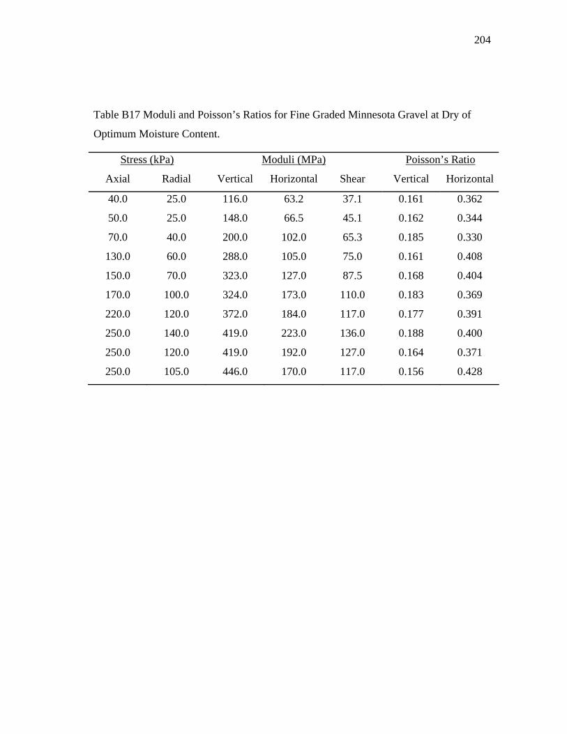
204
Table B17 Moduli and Poisson’s Ratios for Fine Graded Minnesota Gravel at Dry of
Optimum Moisture Content.
Stress (kPa) Moduli (MPa) Poisson’s Ratio
Axial Radial Vertical Horizontal Shear Vertical Horizontal
40.0 25.0 116.0 63.2 37.1 0.161 0.362
50.0 25.0 148.0 66.5 45.1 0.162 0.344
70.0 40.0 200.0 102.0 65.3 0.185 0.330
130.0 60.0 288.0 105.0 75.0 0.161 0.408
150.0 70.0 323.0 127.0 87.5 0.168 0.404
170.0 100.0 324.0 173.0 110.0 0.183 0.369
220.0 120.0 372.0 184.0 117.0 0.177 0.391
250.0 140.0 419.0 223.0 136.0 0.188 0.400
250.0 120.0 419.0 192.0 127.0 0.164 0.371
250.0 105.0 446.0 170.0 117.0 0.156 0.428
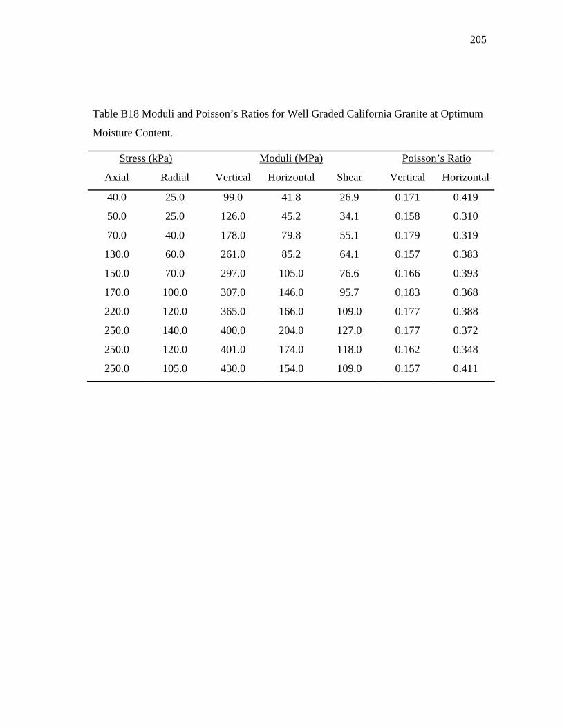
205
Table B18 Moduli and Poisson’s Ratios for Well Graded California Granite at Optimum
Moisture Content.
Stress (kPa) Moduli (MPa) Poisson’s Ratio
Axial Radial Vertical Horizontal Shear Vertical Horizontal
40.0 25.0 99.0 41.8 26.9 0.171 0.419
50.0 25.0 126.0 45.2 34.1 0.158 0.310
70.0 40.0 178.0 79.8 55.1 0.179 0.319
130.0 60.0 261.0 85.2 64.1 0.157 0.383
150.0 70.0 297.0 105.0 76.6 0.166 0.393
170.0 100.0 307.0 146.0 95.7 0.183 0.368
220.0 120.0 365.0 166.0 109.0 0.177 0.388
250.0 140.0 400.0 204.0 127.0 0.177 0.372
250.0 120.0 401.0 174.0 118.0 0.162 0.348
250.0 105.0 430.0 154.0 109.0 0.157 0.411
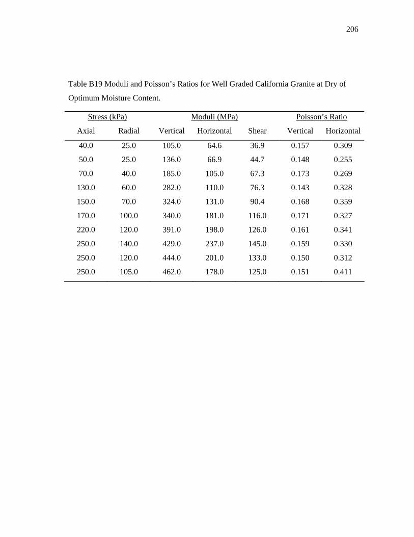
206
Table B19 Moduli and Poisson’s Ratios for Well Graded California Granite at Dry of
Optimum Moisture Content.
Stress (kPa) Moduli (MPa) Poisson’s Ratio
Axial Radial Vertical Horizontal Shear Vertical Horizontal
40.0 25.0 105.0 64.6 36.9 0.157 0.309
50.0 25.0 136.0 66.9 44.7 0.148 0.255
70.0 40.0 185.0 105.0 67.3 0.173 0.269
130.0 60.0 282.0 110.0 76.3 0.143 0.328
150.0 70.0 324.0 131.0 90.4 0.168 0.359
170.0 100.0 340.0 181.0 116.0 0.171 0.327
220.0 120.0 391.0 198.0 126.0 0.161 0.341
250.0 140.0 429.0 237.0 145.0 0.159 0.330
250.0 120.0 444.0 201.0 133.0 0.150 0.312
250.0 105.0 462.0 178.0 125.0 0.151 0.411

207
Table B20 Moduli and Poisson’s Ratios for Well Graded California Granite at Wet of
Optimum Moisture Content.
Stress (kPa) Moduli (MPa) Poisson’s Ratio
Axial Radial Vertical Horizontal Shear Vertical Horizontal
40.0 25.0 101.0 44.0 28.3 0.166 0.354
50.0 25.0 122.0 43.7 32.8 0.158 0.261
70.0 40.0 170.0 75.9 53.5 0.185 0.311
130.0 60.0 276.0 93.4 67.8 0.163 0.375
150.0 70.0 311.0 114.0 81.5 0.155 0.349
170.0 100.0 313.0 161.0 104.0 0.178 0.341
220.0 120.0 381.0 178.0 115.0 0.172 0.365
250.0 140.0 424.0 211.0 136.0 0.170 0.370
250.0 120.0 418.0 179.0 119.0 0.159 0.339
250.0 105.0 457.0 163.0 115.0 0.157 0.417
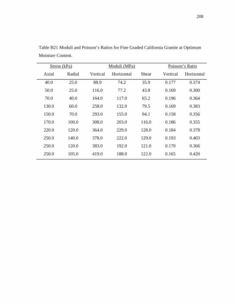
208
Table B21 Moduli and Poisson’s Ratios for Fine Graded California Granite at Optimum
Moisture Content.
Stress (kPa) Moduli (MPa) Poisson’s Ratio
Axial Radial Vertical Horizontal Shear Vertical Horizontal
40.0 25.0 88.9 74.2 35.9 0.177 0.374
50.0 25.0 116.0 77.2 43.8 0.169 0.300
70.0 40.0 164.0 117.0 65.2 0.196 0.364
130.0 60.0 258.0 132.0 79.5 0.169 0.383
150.0 70.0 293.0 155.0 94.1 0.158 0.356
170.0 100.0 308.0 203.0 116.0 0.186 0.355
220.0 120.0 364.0 229.0 128.0 0.184 0.378
250.0 140.0 378.0 222.0 129.0 0.193 0.403
250.0 120.0 383.0 192.0 121.0 0.170 0.366
250.0 105.0 419.0 188.0 122.0 0.165 0.420

209
Table B22 Moduli and Poisson’s Ratios for Fine Graded California Granite at Dry of
Optimum Moisture Content.
Stress (kPa) Moduli (MPa) Poisson’s Ratio
Axial Radial Vertical Horizontal Shear Vertical Horizontal
40.0 25.0 138.0 86.2 48.1 0.170 0.363
50.0 25.0 164.0 92.1 58.6 0.144 0.280
70.0 40.0 210.0 134.0 80.9 0.170 0.297
130.0 60.0 318.0 145.0 94.0 0.162 0.361
150.0 70.0 359.0 175.0 109.0 0.166 0.364
170.0 100.0 362.0 212.0 133.0 0.167 0.334
220.0 120.0 425.0 242.0 143.0 0.171 0.357
250.0 140.0 471.0 283.0 166.0 0.173 0.363
250.0 120.0 463.0 236.0 149.0 0.152 0.337
250.0 105.0 498.0 209.0 142.0 0.154 0.421

210
Table B23 Moduli and Poisson’s Ratios for Fine Graded California Granite at Dry of
Optimum Moisture Content.
Stress (kPa) Moduli (MPa) Poisson’s Ratio
Axial Radial Vertical Horizontal Shear Vertical Horizontal
40.0 25.0 99.0 37.9 26.1 0.197 0.443
50.0 25.0 124.0 46.7 33.5 0.171 0.272
70.0 40.0 166.0 72.6 52.0 0.173 0.312
130.0 60.0 272.0 91.6 65.6 0.153 0.338
150.0 70.0 298.0 108.0 75.9 0.157 0.353
170.0 100.0 299.0 147.0 96.6 0.177 0.311
220.0 120.0 372.0 162.0 108.0 0.170 0.354
250.0 140.0 402.0 195.0 127.0 0.163 0.350
250.0 120.0 422.0 170.0 117.0 0.159 0.330
250.0 105.0 442.0 151.0 110.0 0.146 0.398
211
APPENDIX C
VERTICAL AND HORIZONTAL STRESS DISTRIBUTION
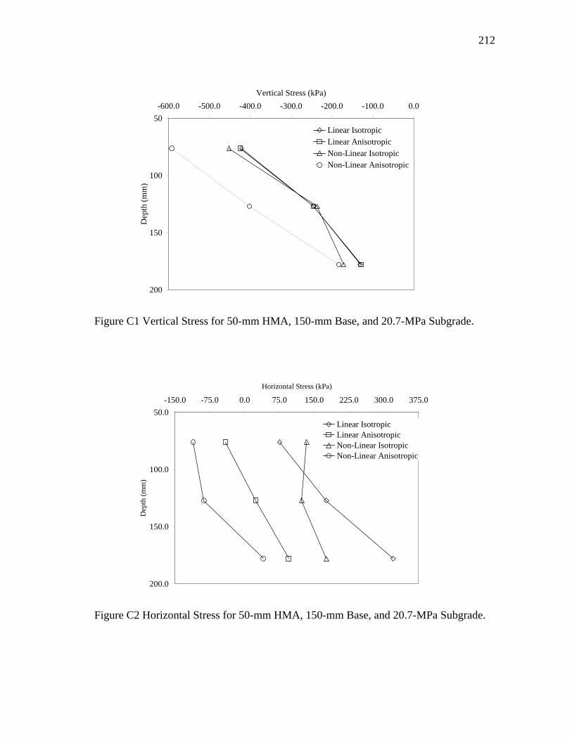
212
50
100
150
200
-600.0 -500.0 -400.0 -300.0 -200.0 -100.0 0.0Vertical Stress (kPa)
Dep
th (m
m)
Linear IsotropicLinear AnisotropicNon-Linear IsotropicNon-Linear Anisotropic
Figure C1 Vertical Stress for 50-mm HMA, 150-mm Base, and 20.7-MPa Subgrade.
50.0
100.0
150.0
200.0
-150.0 -75.0 0.0 75.0 150.0 225.0 300.0 375.0
Horizontal Stress (kPa)
Dep
th (m
m)
Linear IsotropicLinear AnisotropicNon-Linear IsotropicNon-Linear Anisotropic
Figure C2 Horizontal Stress for 50-mm HMA, 150-mm Base, and 20.7-MPa Subgrade.
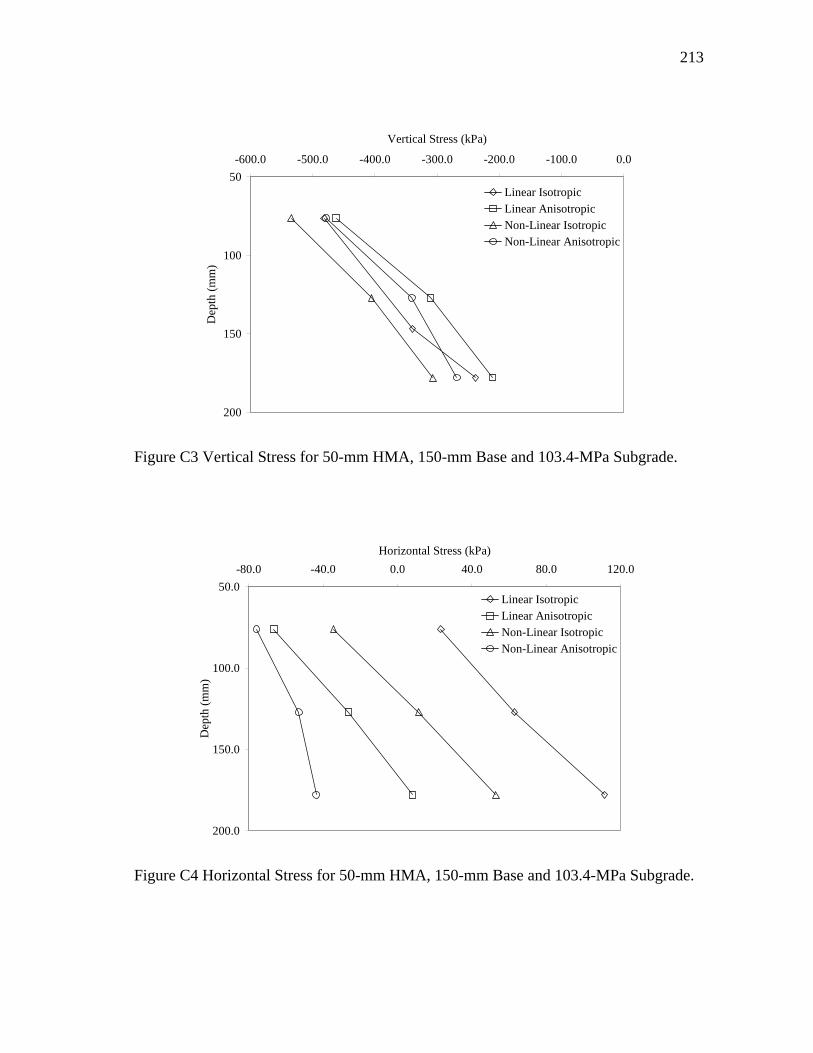
213
50
100
150
200
-600.0 -500.0 -400.0 -300.0 -200.0 -100.0 0.0
Vertical Stress (kPa)
Dep
th (m
m)
Linear IsotropicLinear AnisotropicNon-Linear IsotropicNon-Linear Anisotropic
Figure C3 Vertical Stress for 50-mm HMA, 150-mm Base and 103.4-MPa Subgrade.
50.0
100.0
150.0
200.0
-80.0 -40.0 0.0 40.0 80.0 120.0Horizontal Stress (kPa)
Dep
th (m
m)
Linear IsotropicLinear AnisotropicNon-Linear IsotropicNon-Linear Anisotropic
Figure C4 Horizontal Stress for 50-mm HMA, 150-mm Base and 103.4-MPa Subgrade.
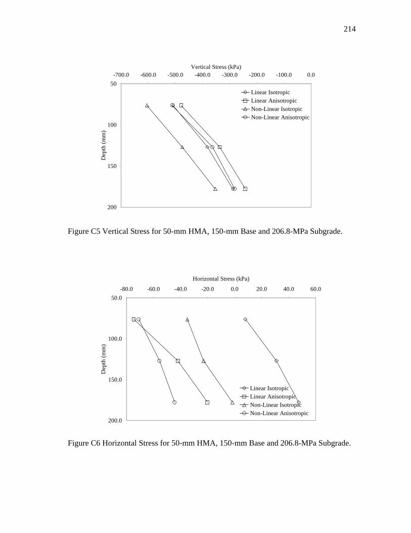
214
50
100
150
200
-700.0 -600.0 -500.0 -400.0 -300.0 -200.0 -100.0 0.0Vertical Stress (kPa)
Dep
th (m
m)
Linear IsotropicLinear AnisotropicNon-Linear IsotropicNon-Linear Anisotropic
Figure C5 Vertical Stress for 50-mm HMA, 150-mm Base and 206.8-MPa Subgrade.
50.0
100.0
150.0
200.0
-80.0 -60.0 -40.0 -20.0 0.0 20.0 40.0 60.0
Horizontal Stress (kPa)
Dep
th (m
m)
Linear IsotropicLinear AnisotropicNon-Linear IsotropicNon-Linear Anisotropic
Figure C6 Horizontal Stress for 50-mm HMA, 150-mm Base and 206.8-MPa Subgrade.
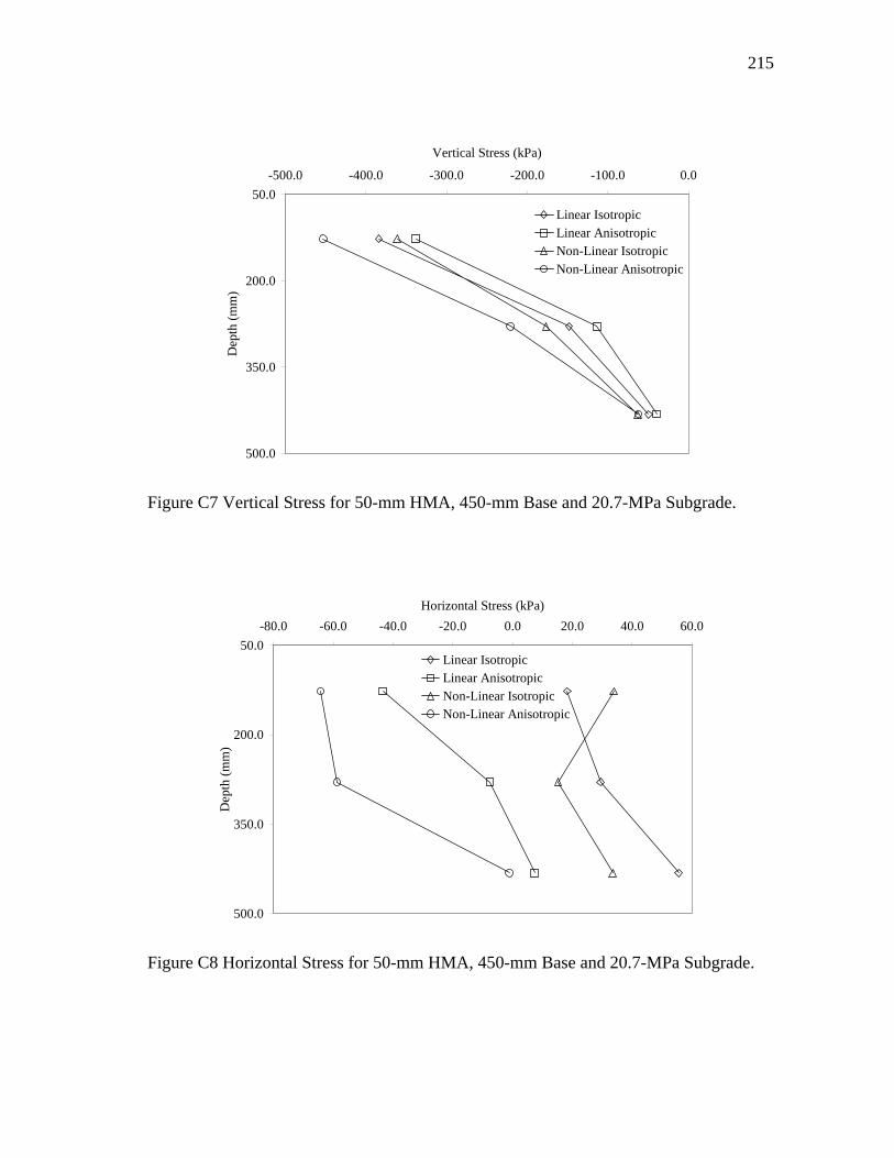
215
50.0
200.0
350.0
500.0
-500.0 -400.0 -300.0 -200.0 -100.0 0.0
Vertical Stress (kPa)
Dep
th (m
m)
Linear IsotropicLinear AnisotropicNon-Linear IsotropicNon-Linear Anisotropic
Figure C7 Vertical Stress for 50-mm HMA, 450-mm Base and 20.7-MPa Subgrade.
50.0
200.0
350.0
500.0
-80.0 -60.0 -40.0 -20.0 0.0 20.0 40.0 60.0Horizontal Stress (kPa)
Dep
th (m
m)
Linear IsotropicLinear AnisotropicNon-Linear IsotropicNon-Linear Anisotropic
Figure C8 Horizontal Stress for 50-mm HMA, 450-mm Base and 20.7-MPa Subgrade.
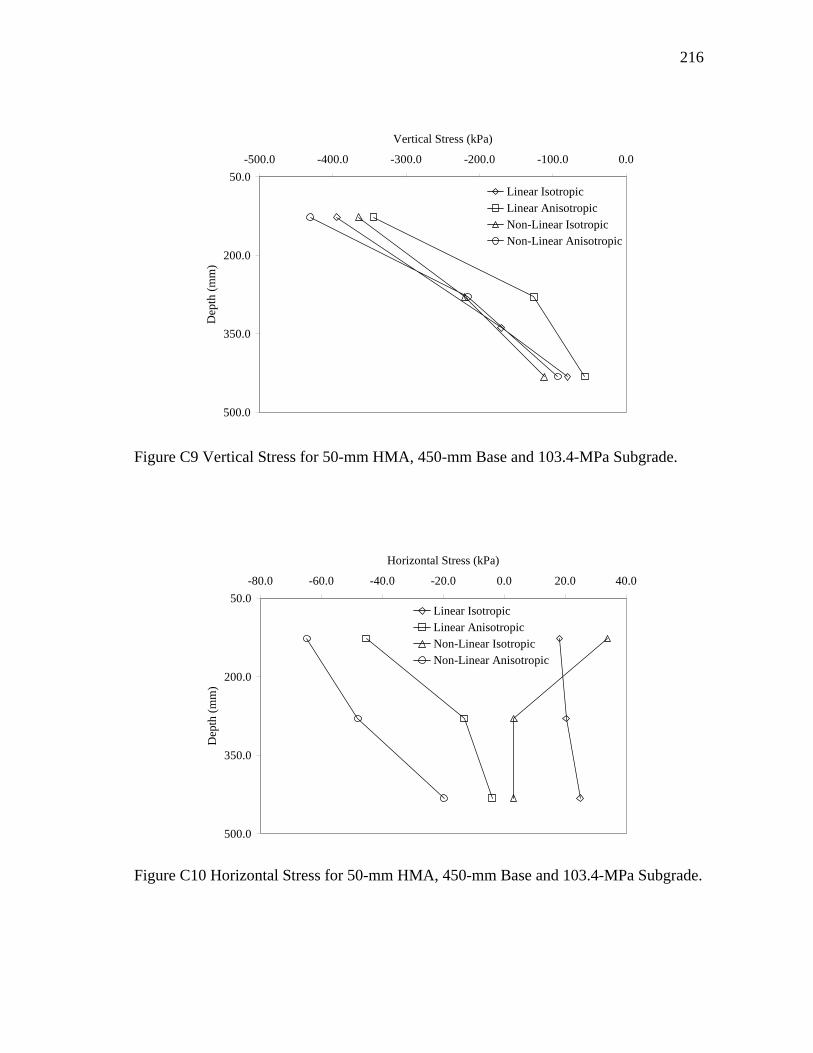
216
50.0
200.0
350.0
500.0
-500.0 -400.0 -300.0 -200.0 -100.0 0.0
Vertical Stress (kPa)
Dep
th (m
m)
Linear IsotropicLinear AnisotropicNon-Linear IsotropicNon-Linear Anisotropic
Figure C9 Vertical Stress for 50-mm HMA, 450-mm Base and 103.4-MPa Subgrade.
50.0
200.0
350.0
500.0
-80.0 -60.0 -40.0 -20.0 0.0 20.0 40.0
Horizontal Stress (kPa)
Dep
th (m
m)
Linear IsotropicLinear AnisotropicNon-Linear IsotropicNon-Linear Anisotropic
Figure C10 Horizontal Stress for 50-mm HMA, 450-mm Base and 103.4-MPa Subgrade.
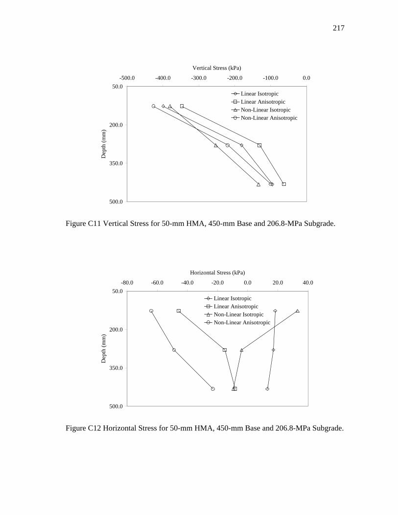
217
50.0
200.0
350.0
500.0
-500.0 -400.0 -300.0 -200.0 -100.0 0.0
Vertical Stress (kPa)
Dep
th (m
m)
Linear IsotropicLinear AnisotropicNon-Linear IsotropicNon-Linear Anisotropic
Figure C11 Vertical Stress for 50-mm HMA, 450-mm Base and 206.8-MPa Subgrade.
50.0
200.0
350.0
500.0
-80.0 -60.0 -40.0 -20.0 0.0 20.0 40.0
Horizontal Stress (kPa)
Dep
th (m
m)
Linear IsotropicLinear AnisotropicNon-Linear IsotropicNon-Linear Anisotropic
Figure C12 Horizontal Stress for 50-mm HMA, 450-mm Base and 206.8-MPa Subgrade.
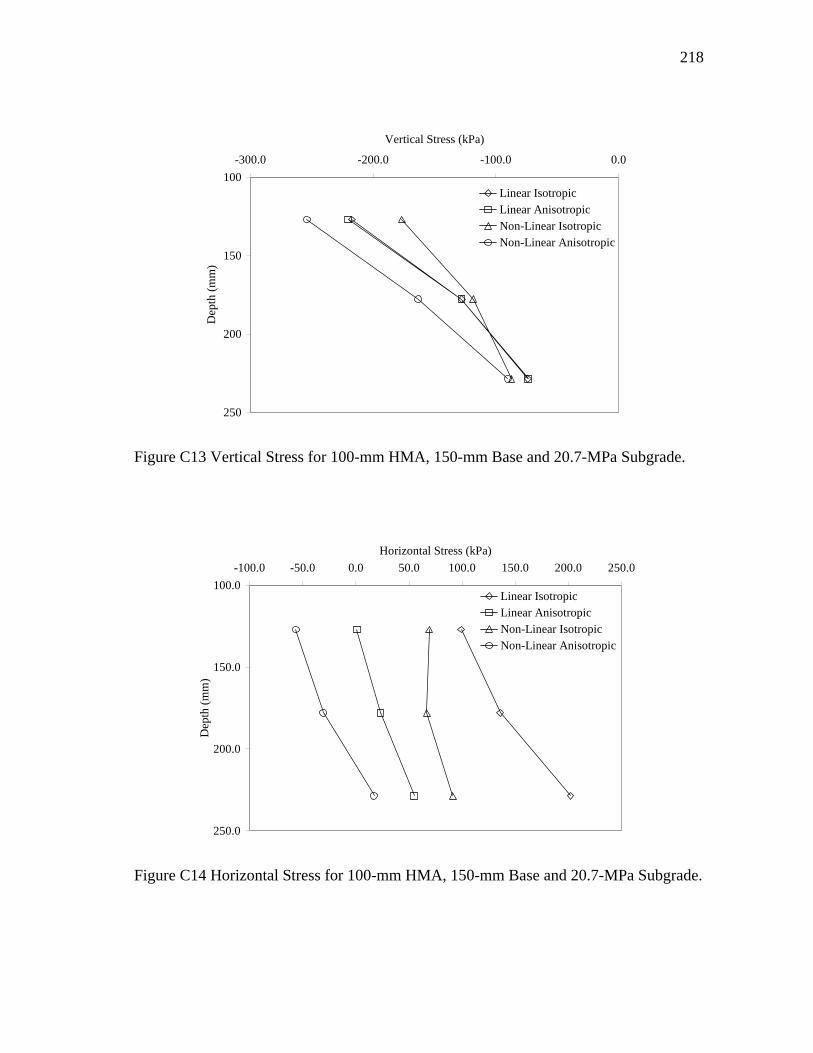
218
100
150
200
250
-300.0 -200.0 -100.0 0.0
Vertical Stress (kPa)
Dep
th (m
m)
Linear IsotropicLinear AnisotropicNon-Linear IsotropicNon-Linear Anisotropic
Figure C13 Vertical Stress for 100-mm HMA, 150-mm Base and 20.7-MPa Subgrade.
100.0
150.0
200.0
250.0
-100.0 -50.0 0.0 50.0 100.0 150.0 200.0 250.0Horizontal Stress (kPa)
Dep
th (m
m)
Linear IsotropicLinear AnisotropicNon-Linear IsotropicNon-Linear Anisotropic
Figure C14 Horizontal Stress for 100-mm HMA, 150-mm Base and 20.7-MPa Subgrade.
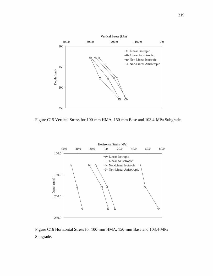
219
100
150
200
250
-400.0 -300.0 -200.0 -100.0 0.0
Vertical Stress (kPa)
Dep
th (m
m)
Linear IsotropicLinear AnisotropicNon-Linear IsotropicNon-Linear Anisotropic
Figure C15 Vertical Stress for 100-mm HMA, 150-mm Base and 103.4-MPa Subgrade.
100.0
150.0
200.0
250.0
-60.0 -40.0 -20.0 0.0 20.0 40.0 60.0 80.0Horizontal Stress (kPa)
Dep
th (m
m)
Linear IsotropicLinear AnisotropicNon-Linear IsotropicNon-Linear Anisotropic
Figure C16 Horizontal Stress for 100-mm HMA, 150-mm Base and 103.4-MPa
Subgrade.
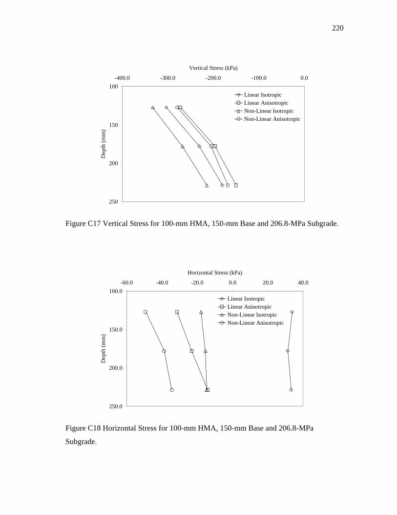
220
100
150
200
250
-400.0 -300.0 -200.0 -100.0 0.0
Vertical Stress (kPa)
Dep
th (m
m)
Linear IsotropicLinear AnisotropicNon-Linear IsotropicNon-Linear Anisotropic
Figure C17 Vertical Stress for 100-mm HMA, 150-mm Base and 206.8-MPa Subgrade.
100.0
150.0
200.0
250.0
-60.0 -40.0 -20.0 0.0 20.0 40.0
Horizontal Stress (kPa)
Dep
th (m
m)
Linear IsotropicLinear AnisotropicNon-Linear IsotropicNon-Linear Anisotropic
Figure C18 Horizontal Stress for 100-mm HMA, 150-mm Base and 206.8-MPa
Subgrade.
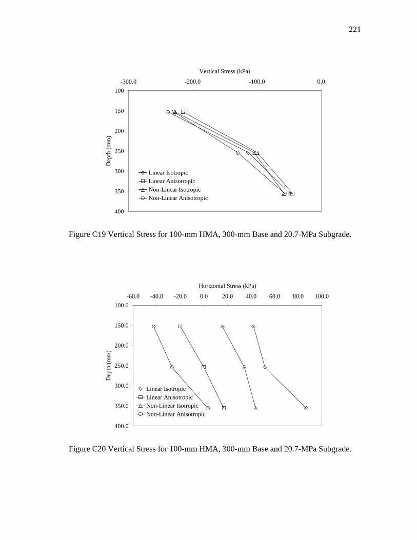
221
100
150
200
250
300
350
400
-300.0 -200.0 -100.0 0.0
Vertical Stress (kPa)
Dep
th (m
m)
Linear IsotropicLinear AnisotropicNon-Linear IsotropicNon-Linear Anisotropic
Figure C19 Vertical Stress for 100-mm HMA, 300-mm Base and 20.7-MPa Subgrade.
100.0
150.0
200.0
250.0
300.0
350.0
400.0
-60.0 -40.0 -20.0 0.0 20.0 40.0 60.0 80.0 100.0
Horizontal Stress (kPa)
Dep
th (m
m)
Linear IsotropicLinear AnisotropicNon-Linear IsotropicNon-Linear Anisotropic
Figure C20 Vertical Stress for 100-mm HMA, 300-mm Base and 20.7-MPa Subgrade.
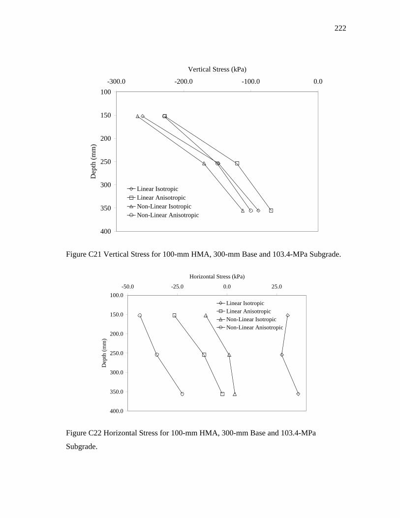
222
100
150
200
250
300
350
400
-300.0 -200.0 -100.0 0.0
Vertical Stress (kPa)
Dep
th (m
m)
Linear IsotropicLinear AnisotropicNon-Linear IsotropicNon-Linear Anisotropic
Figure C21 Vertical Stress for 100-mm HMA, 300-mm Base and 103.4-MPa Subgrade.
100.0
150.0
200.0
250.0
300.0
350.0
400.0
-50.0 -25.0 0.0 25.0
Horizontal Stress (kPa)
Dep
th (m
m)
Linear IsotropicLinear AnisotropicNon-Linear IsotropicNon-Linear Anisotropic
Figure C22 Horizontal Stress for 100-mm HMA, 300-mm Base and 103.4-MPa
Subgrade.
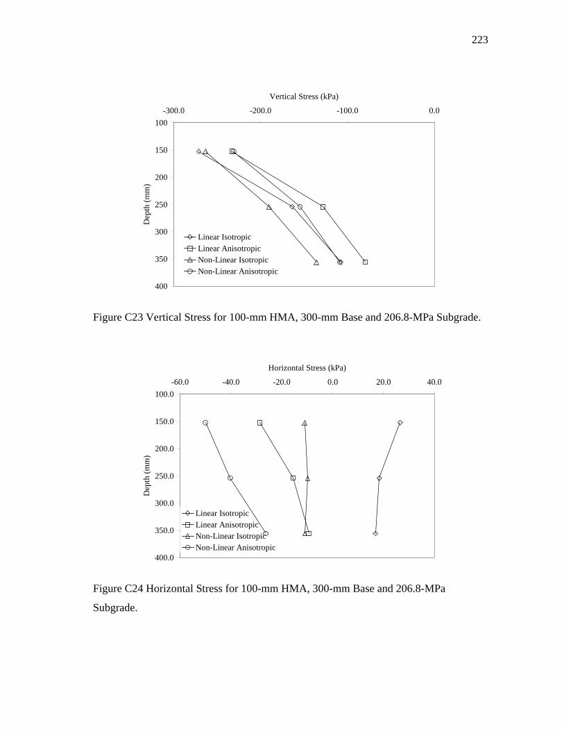
223
100
150
200
250
300
350
400
-300.0 -200.0 -100.0 0.0
Vertical Stress (kPa)
Dep
th (m
m)
Linear IsotropicLinear AnisotropicNon-Linear IsotropicNon-Linear Anisotropic
Figure C23 Vertical Stress for 100-mm HMA, 300-mm Base and 206.8-MPa Subgrade.
100.0
150.0
200.0
250.0
300.0
350.0
400.0
-60.0 -40.0 -20.0 0.0 20.0 40.0
Horizontal Stress (kPa)
Dep
th (m
m)
Linear IsotropicLinear AnisotropicNon-Linear IsotropicNon-Linear Anisotropic
Figure C24 Horizontal Stress for 100-mm HMA, 300-mm Base and 206.8-MPa
Subgrade.
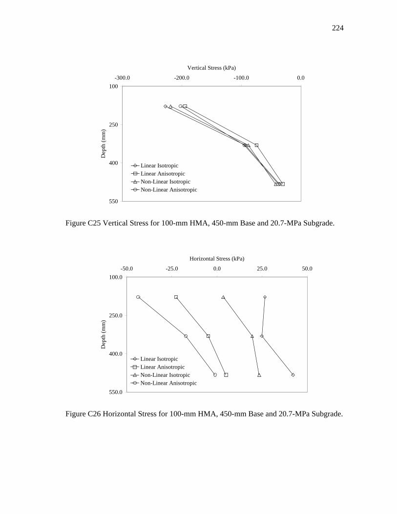
224
100
250
400
550
-300.0 -200.0 -100.0 0.0
Vertical Stress (kPa)
Dep
th (m
m)
Linear IsotropicLinear AnisotropicNon-Linear IsotropicNon-Linear Anisotropic
Figure C25 Vertical Stress for 100-mm HMA, 450-mm Base and 20.7-MPa Subgrade.
100.0
250.0
400.0
550.0
-50.0 -25.0 0.0 25.0 50.0
Horizontal Stress (kPa)
Dep
th (m
m)
Linear IsotropicLinear AnisotropicNon-Linear IsotropicNon-Linear Anisotropic
Figure C26 Horizontal Stress for 100-mm HMA, 450-mm Base and 20.7-MPa Subgrade.

225
100
250
400
550
-300.0 -200.0 -100.0 0.0
Vertical Stress (kPa)
Dep
th (m
m)
Linear IsotropicLinear AnisotropicNon-Linear IsotropicNon-Linear Anisotropic
Figure C27 Vertical Stress for 100-mm HMA, 450-mm Base and 103.4-MPa Subgrade.
100.0
250.0
400.0
550.0
-50.0 -25.0 0.0 25.0 50.0
Horizontal Stress (kPa)
Dep
th (m
m)
Linear IsotropicLinear AnisotropicNon-Linear IsotropicNon-Linear Anisotropic
Figure C28 Horizontal Stress for 100-mm HMA, 450-mm Base and 103.4-MPa
Subgrade.
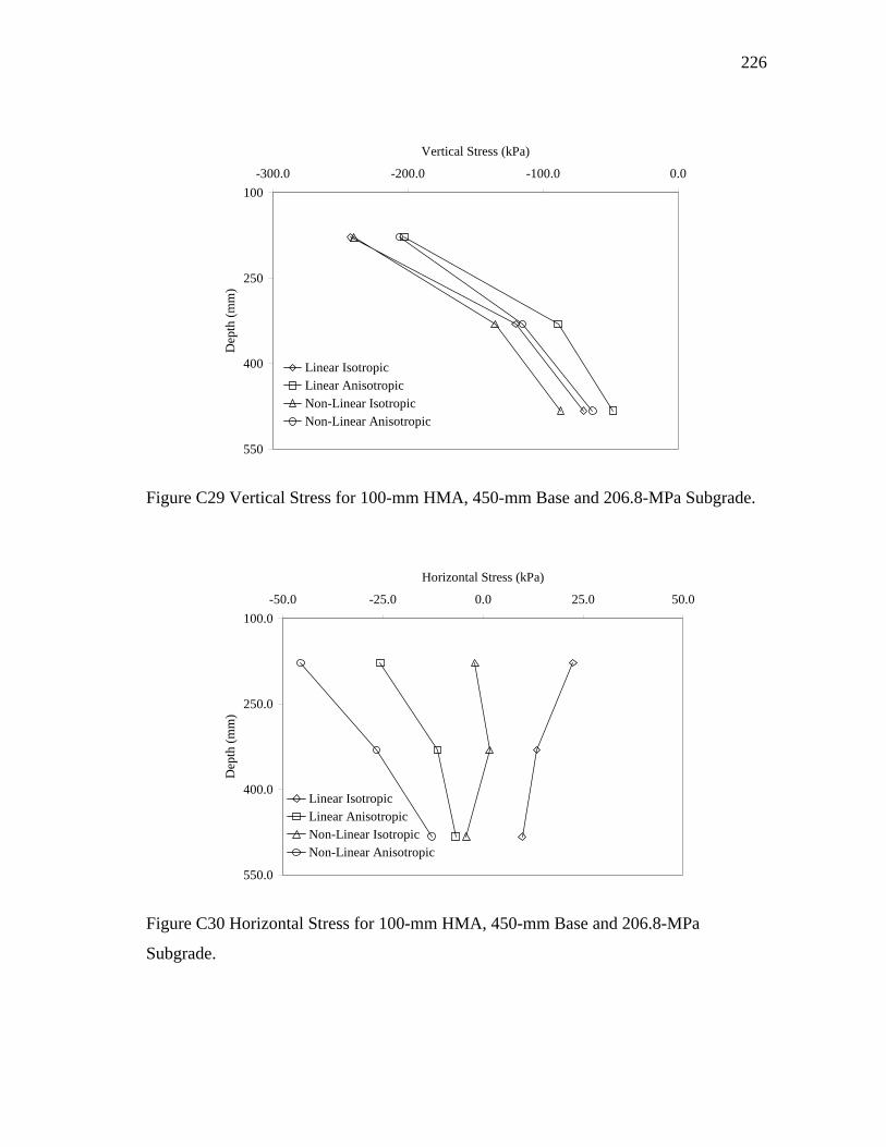
226
100
250
400
550
-300.0 -200.0 -100.0 0.0
Vertical Stress (kPa)
Dep
th (m
m)
Linear IsotropicLinear AnisotropicNon-Linear IsotropicNon-Linear Anisotropic
Figure C29 Vertical Stress for 100-mm HMA, 450-mm Base and 206.8-MPa Subgrade.
100.0
250.0
400.0
550.0
-50.0 -25.0 0.0 25.0 50.0
Horizontal Stress (kPa)
Dep
th (m
m)
Linear IsotropicLinear AnisotropicNon-Linear IsotropicNon-Linear Anisotropic
Figure C30 Horizontal Stress for 100-mm HMA, 450-mm Base and 206.8-MPa
Subgrade.
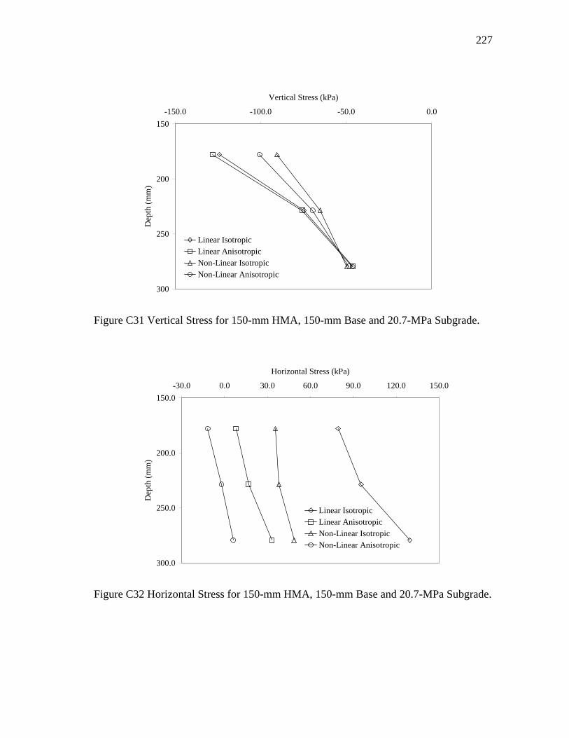
227
150
200
250
300
-150.0 -100.0 -50.0 0.0
Vertical Stress (kPa)
Dep
th (m
m)
Linear IsotropicLinear AnisotropicNon-Linear IsotropicNon-Linear Anisotropic
Figure C31 Vertical Stress for 150-mm HMA, 150-mm Base and 20.7-MPa Subgrade.
150.0
200.0
250.0
300.0
-30.0 0.0 30.0 60.0 90.0 120.0 150.0
Horizontal Stress (kPa)
Dep
th (m
m)
Linear IsotropicLinear AnisotropicNon-Linear IsotropicNon-Linear Anisotropic
Figure C32 Horizontal Stress for 150-mm HMA, 150-mm Base and 20.7-MPa Subgrade.
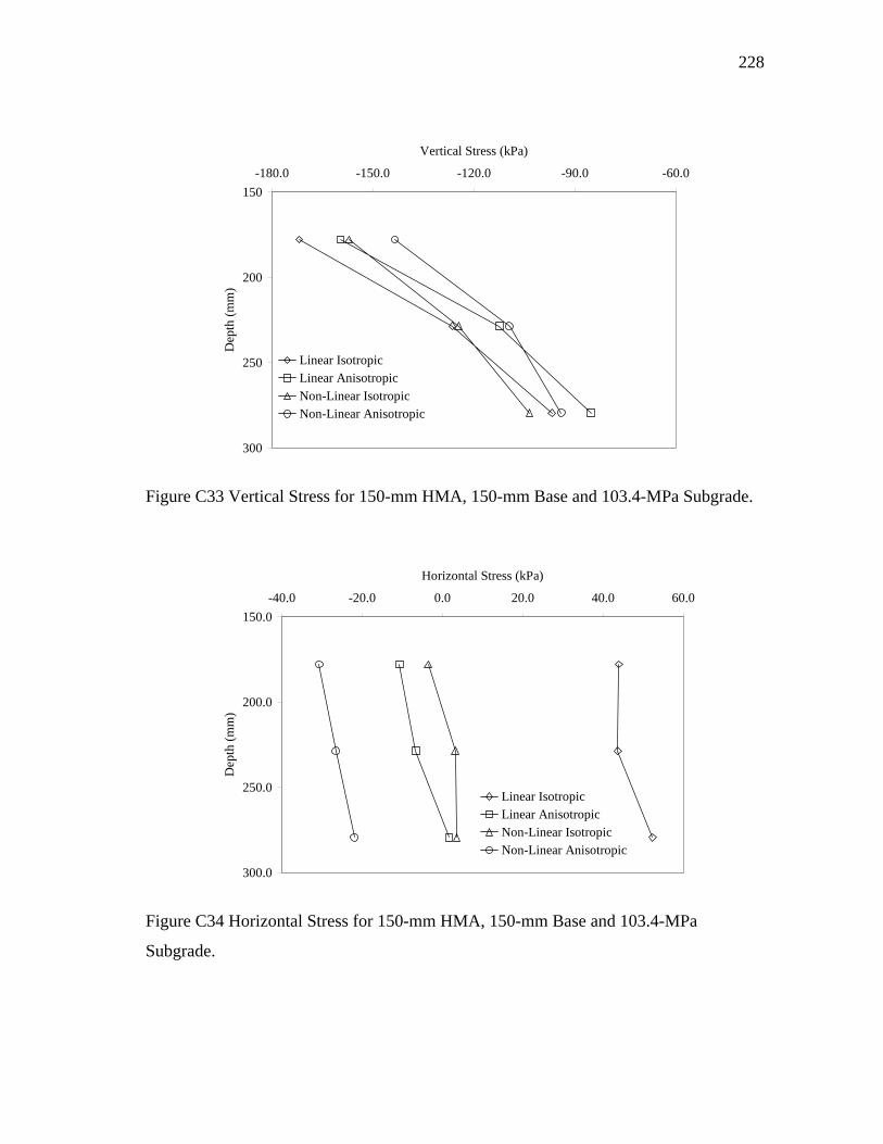
228
150
200
250
300
-180.0 -150.0 -120.0 -90.0 -60.0
Vertical Stress (kPa)
Dep
th (m
m)
Linear IsotropicLinear AnisotropicNon-Linear IsotropicNon-Linear Anisotropic
Figure C33 Vertical Stress for 150-mm HMA, 150-mm Base and 103.4-MPa Subgrade.
150.0
200.0
250.0
300.0
-40.0 -20.0 0.0 20.0 40.0 60.0
Horizontal Stress (kPa)
Dep
th (m
m)
Linear IsotropicLinear AnisotropicNon-Linear IsotropicNon-Linear Anisotropic
Figure C34 Horizontal Stress for 150-mm HMA, 150-mm Base and 103.4-MPa
Subgrade.
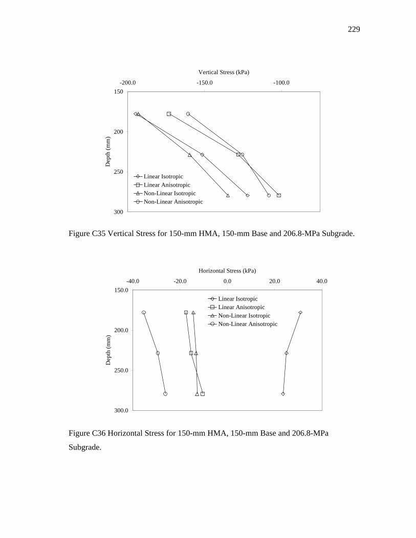
229
150
200
250
300
-200.0 -150.0 -100.0
Vertical Stress (kPa)
Dep
th (m
m)
Linear IsotropicLinear AnisotropicNon-Linear IsotropicNon-Linear Anisotropic
Figure C35 Vertical Stress for 150-mm HMA, 150-mm Base and 206.8-MPa Subgrade.
150.0
200.0
250.0
300.0
-40.0 -20.0 0.0 20.0 40.0
Horizontal Stress (kPa)
Dep
th (m
m)
Linear IsotropicLinear AnisotropicNon-Linear IsotropicNon-Linear Anisotropic
Figure C36 Horizontal Stress for 150-mm HMA, 150-mm Base and 206.8-MPa
Subgrade.
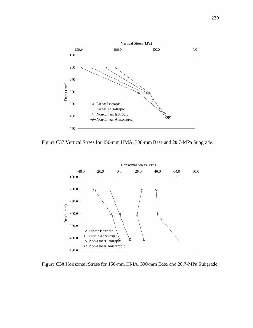
230
150
200
250
300
350
400
450
-150.0 -100.0 -50.0 0.0
Vertical Stress (kPa)
Dep
th (m
m)
Linear IsotropicLinear AnisotropicNon-Linear IsotropicNon-Linear Anisotropic
Figure C37 Vertical Stress for 150-mm HMA, 300-mm Base and 20.7-MPa Subgrade.
150.0
200.0
250.0
300.0
350.0
400.0
450.0
-40.0 -20.0 0.0 20.0 40.0 60.0 80.0
Horizontal Stress (kPa)
Dep
th (m
m)
Linear IsotropicLinear AnisotropicNon-Linear IsotropicNon-Linear Anisotropic
Figure C38 Horizontal Stress for 150-mm HMA, 300-mm Base and 20.7-MPa Subgrade.
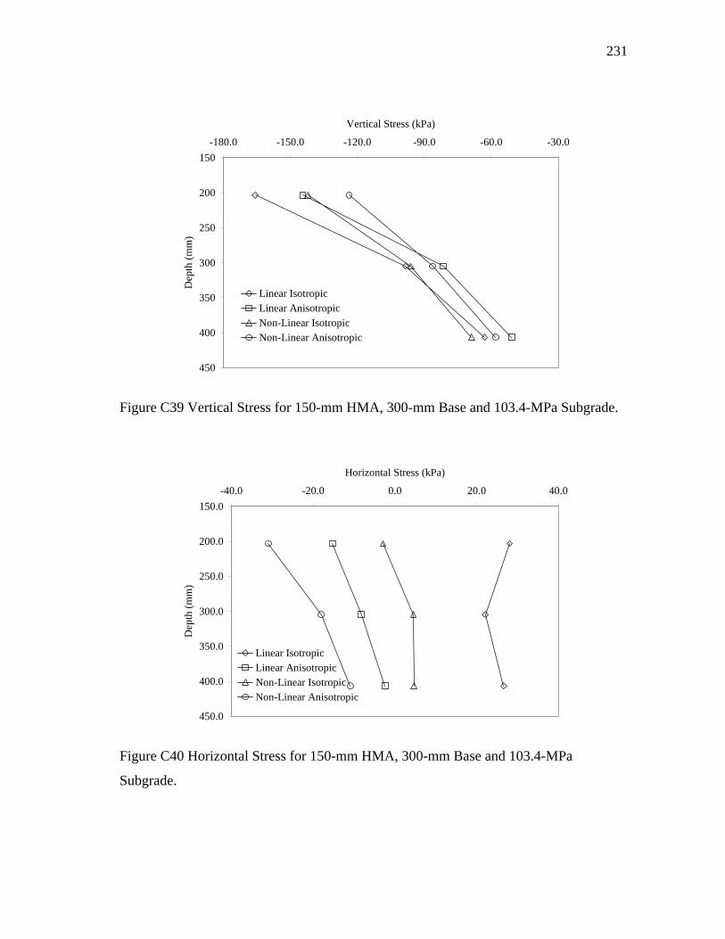
231
150
200
250
300
350
400
450
-180.0 -150.0 -120.0 -90.0 -60.0 -30.0
Vertical Stress (kPa)
Dep
th (m
m)
Linear IsotropicLinear AnisotropicNon-Linear IsotropicNon-Linear Anisotropic
Figure C39 Vertical Stress for 150-mm HMA, 300-mm Base and 103.4-MPa Subgrade.
150.0
200.0
250.0
300.0
350.0
400.0
450.0
-40.0 -20.0 0.0 20.0 40.0
Horizontal Stress (kPa)
Dep
th (m
m)
Linear IsotropicLinear AnisotropicNon-Linear IsotropicNon-Linear Anisotropic
Figure C40 Horizontal Stress for 150-mm HMA, 300-mm Base and 103.4-MPa
Subgrade.

232
150
200
250
300
350
400
450
-200.0 -150.0 -100.0 -50.0
Vertical Stress (kPa)
Dep
th (m
m)
Linear IsotropicLinear AnisotropicNon-Linear IsotropicNon-Linear Anisotropic
Figure C41 Vertical Stress for 150-mm HMA, 300-mm Base and 206.8-MPa Subgrade.
150.0
200.0
250.0
300.0
350.0
400.0
450.0
-40.0 -20.0 0.0 20.0
Horizontal Stress (kPa)
Dep
th (m
m)
Linear IsotropicLinear AnisotropicNon-Linear IsotropicNon-Linear Anisotropic
Figure C42 Horizontal Stress for 150-mm HMA, 300-mm Base and 206.8-MPa
Subgrade.
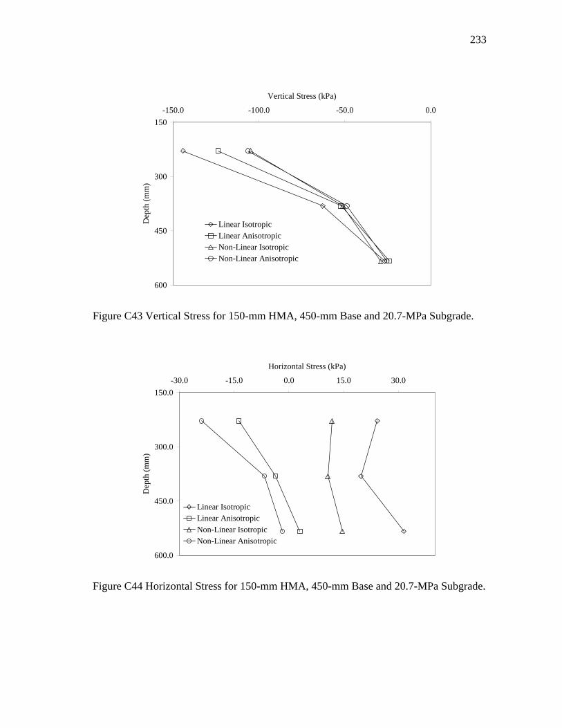
233
150
300
450
600
-150.0 -100.0 -50.0 0.0
Vertical Stress (kPa)
Dep
th (m
m)
Linear IsotropicLinear AnisotropicNon-Linear IsotropicNon-Linear Anisotropic
Figure C43 Vertical Stress for 150-mm HMA, 450-mm Base and 20.7-MPa Subgrade.
150.0
300.0
450.0
600.0
-30.0 -15.0 0.0 15.0 30.0
Horizontal Stress (kPa)
Dep
th (m
m)
Linear IsotropicLinear AnisotropicNon-Linear IsotropicNon-Linear Anisotropic
Figure C44 Horizontal Stress for 150-mm HMA, 450-mm Base and 20.7-MPa Subgrade.
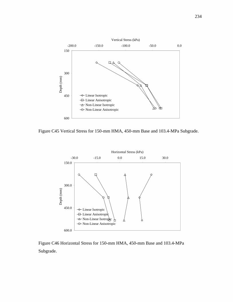
234
150
300
450
600
-200.0 -150.0 -100.0 -50.0 0.0
Vertical Stress (kPa)
Dep
th (m
m)
Linear IsotropicLinear AnisotropicNon-Linear IsotropicNon-Linear Anisotropic
Figure C45 Vertical Stress for 150-mm HMA, 450-mm Base and 103.4-MPa Subgrade.
150.0
300.0
450.0
600.0
-30.0 -15.0 0.0 15.0 30.0
Horizontal Stress (kPa)
Dep
th (m
m)
Linear IsotropicLinear AnisotropicNon-Linear IsotropicNon-Linear Anisotropic
Figure C46 Horizontal Stress for 150-mm HMA, 450-mm Base and 103.4-MPa
Subgrade.
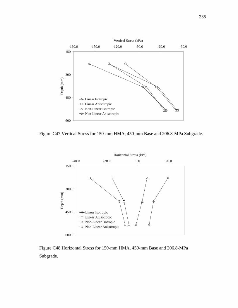
235
150
300
450
600
-180.0 -150.0 -120.0 -90.0 -60.0 -30.0
Vertical Stress (kPa)
Dep
th (m
m)
Linear IsotropicLinear AnisotropicNon-Linear IsotropicNon-Linear Anisotropic
Figure C47 Vertical Stress for 150-mm HMA, 450-mm Base and 206.8-MPa Subgrade.
150.0
300.0
450.0
600.0
-40.0 -20.0 0.0 20.0
Horizontal Stress (kPa)
Dep
th (m
m)
Linear IsotropicLinear AnisotropicNon-Linear IsotropicNon-Linear Anisotropic
Figure C48 Horizontal Stress for 150-mm HMA, 450-mm Base and 206.8-MPa
Subgrade.


