ECOHYDROLOGYEcohydrol. (2010)Published online in Wiley Online Library(wileyonlinelibrary.com) DOI: 10.1002/eco.187

Characterizing ecohydrological and biogeochemicalconnectivity across multiple scales: a new conceptual

framework

Lixin Wang,1* Chris Zou,2 Frances O’Donnell,1 Stephen Good,1 Trenton Franz,1

Gretchen R. Miller,3 Kelly K. Caylor,1 Jessica M. Cable4 and Barbara Bond5

1 Department of Civil and Environmental Engineering, Princeton University, Princeton, NJ 08544, USA2 Department of Natural Resource Ecology and Management, Oklahoma State University, Stillwater, OK, USA

3 Department of Civil Engineering, Texas A&M University, College Station, TX, USA4 International Arctic Research Center, University of Alaska, Fairbanks, AK, USA

5 Department of Forest Ecosystems and Society, Oregon State University, Corvallis, OR 97331, USA

ABSTRACT

The connectivity of ecohydrological and biogeochemical processes across time and space is a critical determinant of ecosystemstructure and function. However, characterizing cross-scale connectivity is a challenge due to the lack of theories and modellingapproaches that are applicable at multiple scales and due to our rudimentary understanding of the magnitude and dynamicsof such connectivity. In this article, we present a conceptual framework for upscaling quantitative models of ecohydrologicaland biogeochemical processes using electrical circuit analogies and the Thevenin’s theorem. Any process with a feasiblelinear electrical circuit analogy can be represented in larger scale models as a simplified Thevenin equivalent. The Theveninequivalent behaves identically to the original circuit, so the mechanistic features of the model are maintained at largerscales. We present three case applications: water transport, carbon transport, and nitrogen transport. These examples showthat Thevenin’s theorem could be a useful tool for upscaling models of interconnected ecohydrological and biogeochemicalsystems. It is also possible to investigate how disruptions in micro-scale connectivity can affect macro-scale processes. Theutility of the Thevenin’s theorem in environmental sciences is somewhat limited, because not all processes can be representedas linear electrical circuits. However, where it is applicable, it provides an inherently scalable and quantitative framework fordescribing ecohydrological connectivity. Copyright 2010 John Wiley & Sons, Ltd.

KEY WORDS carbon cycling; electrical circuit; nitrogen cycling; nutrient cycling; scaling; soil-plant-atmosphere continuum;Thevenin’s theorem; watershed

Received 12 August 2010; Accepted 17 November 2010

INTRODUCTION

Connectivity has different definitions in various disci-plines. For example, in population studies, connectivity isthe degree to which the landscape facilitates or impedesmovement among resource patches (Taylor et al., 1993;Tischendorf and Fahrig, 2000); in network communica-tion, connectivity refers to the status that network remainsconnected so that information collected by sensor nodescan be relayed back to data sinks or controllers (Zhangand Hou, 2005). Recently, the connectivity concept hasbeen applied to various physical processes within andamong ecosystems to better understand system dynam-ics at large scales (Peters et al., 2006), although it is notaccurately defined in ecosystem studies. The working def-inition of connectivity in this article is the connections inecological or hydrological processes that appear withinor among different spatial scales.

The abiotic media that connect environmental systemsinclude carbon, water, nutrients, energy, and momentum,

* Correspondence to: Lixin Wang, Department of Civil and Environmen-tal Engineering, Princeton University, Princeton, NJ 08544, USA.E-mail: lixinw@princeton.edu

as well as the interactions among them (Austin et al.,2004; Wang et al., 2009). One of the major advantagesof studying connectivity in physical processes is to under-stand the cross-scale interactions. For example, howdo variations of ribulose-1,5-bisphosphate carboxylase-oxygenase (RuBisCo) function in C3 and C4 plants affectlandscape scale CO2 fluxes. This knowledge will signif-icantly improve our system predictions at larger scalebased on information from smaller scales (Peters et al.,2004). However, quantifying cross-scale connectivity isstill a major challenge due largely to the lack of theoriesand modelling approaches that are applicable at multiplescales. Analogical models offer a potential approach forquantifying cross-scale connectivity, which simulate thebehaviours of complex physical systems using laws andtheorems known to control component processes. Suchmodels have been successfully applied to simulate flowsof matter and energy in environmental systems. A well-known example of analogical modelling in environmentalscience is the parallel between Ohm’s law for electric cur-rent flow (Honert, 1948) and Darcy’s law (phenomeno-logically derived constitutive equation that describes the

Copyright 2010 John Wiley & Sons, Ltd.

L. WANG et al.

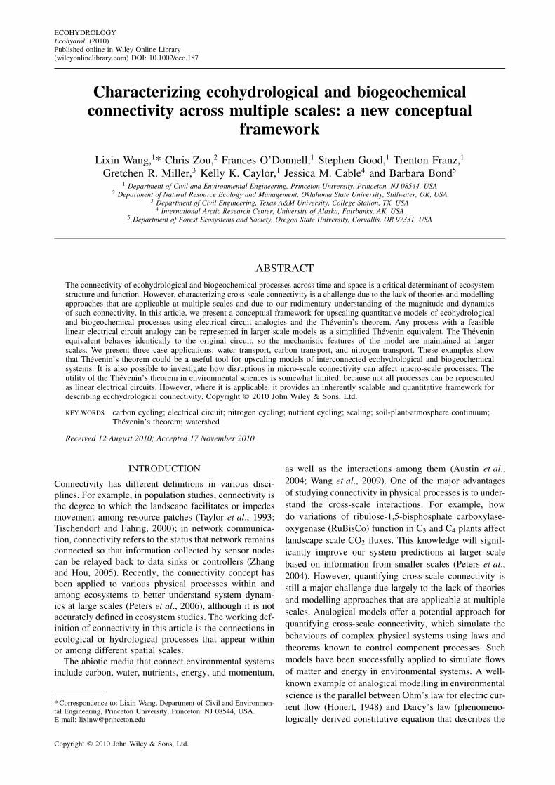
Figure 1. An example of application of Thevenin’s theorem to simplify electrical circuit. R1 to R7 are resistors, V1 and V2 are voltage source, andI1 and I2 are current source. RT and VT are the corresponding Thevenin equivalents solved based on the Thevenin’s theorem.

flow of a fluid through a porous medium) for groundwa-ter flow (Dingman, 2008). The description of biophysicalprocesses with electrical circuit theory has many otherapplications in the environmental sciences, including themodelling of evapotranspiration as the resistance termsin the Penman–Monteith equation (Jones, 1992).

In this article, we formulate analogical models that areable to connect biophysical processes acting at differ-ent scales through a consistent framework. The paradigmmay provide insight into landscape connectivity as well asinteractions between micro- and macro-scale ecohydro-logical and biogeochemical processes. Specifically, ourobjective is to evaluate the applicability of using electricalcircuit analogies and the Thevenin’s theorem to upscaleconnectivity in a quantitative manner. Although the theo-rem has been applied in electrical circuit theory for overa century, its application in the environmental sciences isrelatively new (Campbell, 2003).

The Thevenin’s theorem is used to simplify electricalcircuits. It states that any linear combination of voltagesources, current sources, and resistances can be equiva-lently represented by one resistor in series with one volt-age source (Dorf and Svoboda, 2006). Therefore, ecosys-tem processes with linear electrical analogies could berepresented by their Thevenin equivalents in larger scalemodels. This allows detailed interactions at a small scaleto be represented simply when scaling up. The represen-tation of hydrological systems with electrical analogieshas a long history in the environmental sciences (e.g.resistance terms in Penman–Monteith equation). TheThevenin’s theorem would provide new opportunities forusing electrical analogies to systematically describe andquantify connectivity should this framework prove to bepractically achievable over a wide range of processes.

Thevenin’s theorem: concept and principles

A key set of theorems from electrical circuit theory arethe Thevenin’s and Norton’s theorems that allow for

linear circuits of resistors, current sources, and voltagesources of any size and configuration with two terminalsto be represented by a single resistor and a single voltagesource in series (Thevenin’s theorem) or a single resistorand a single current source in parallel (Norton’s theorem)(Boylestad, 1982). The simplified ‘equivalent circuit’behaves exactly as the larger circuit from the voltagepoint of the connecting terminals (Dorf and Svoboda,2006) (Figure 1). Campbell (2003) applied Thevenin’stheorem to an electrical circuit model of sensible andlatent heat flux from plant canopies, representing theflux of enthalpy and isothermal latent heat with asingle resistor and voltage source for each componentflux. In this work, we demonstrate the broad potentialuse of the Thevenin’s theorem to represent differentecological/hydrological processes (e.g. root water uptakeand carbon fixation at cell level) at small scales witha simplified equivalent circuit, then subsequently usethese equivalent circuits as building blocks of analogynetworks representing processes at larger scales (e.g.watershed scale leaching). In this fashion, we are ableto maintain representation of process at the micro-scalewhen modelling at the macro-scale.

Application of the Thevenin’s theorem involves twosteps. First, the two terminals are connected with anopen circuit, and the voltage across the open connectionis calculated as the Thevenin equivalent voltage (Vth).Second, any independent sources are deactivated andthe Thevenin resistance (Rth) is found through circuitresistance reduction. The Thevenin equivalent circuit isthen made of one ideal voltage source (Vth) in series witha single resistor (Rth). More complicated cases involvingindependent and dependent sources may also be resolvedinto a Thevenin equivalent circuit, and the reader isdirected to introductory circuit analysis texts for furtherinformation (Boylestad, 1982; Dorf and Svoboda, 2006).In the event that the particular configuration of the circuitin question is not known, the Thevenin equivalent may

Copyright 2010 John Wiley & Sons, Ltd. Ecohydrol. (2010)

CHARACTERIZE CONNECTIVITY ACROSS SCALES

Table I. Electrical analogies to ecohydrological and biogeochemical parameters and the corresponding units.

Water Carbon Nitrogen

Voltage (V) Water potential difference, (Pa)

Concentration difference of carboncompounds (mol/m3)

Concentration difference ofnitrogen compounds (mol/m3)

Current (I) Mass flow through system, Q(kg/m2/s)

Carbon flux density (mol/m2/s) Nitrogen flux density (mol/m2/s)

Resistance (R) Resistance to water movementthrough soil pores, plantxylem, and theleaf–atmosphere interface(kg/m2/ Pa)

Impedance to carbon flow of a linkin the system (s/m)

Impedance to nitrogen flow of alink in the system (s/m)

still be determined. For example, in the laboratory, avariable resistor and voltmeter can be connected to theterminals of the circuit in question, and a series of voltagemeasurements are then taken for different resistor values.Voltage is then plotted as a function of resistance, and aline fit to the data. The slope of this line is then Vth andthe intercept is Rth (Dorf and Svoboda, 2006).

In the following sections, we evaluate the applicabilityof the Thevenin’s theorem to three processes acrossmultiple scales: water transport, carbon transport, andnitrogen transport.

Case applications

Case I—water transport in plant, hillslope and water-shed. Water transport processes define critical ecohydro-logical interactions and connections. Substantial progresshas been made in terms of understanding how water fluxand transport affects ecological processes and vegetationdynamics and vice versa. The integrated understandingof ecohydrological interactions and connections at multi-ple scales will help solve issues related to land use, landcover, and climate changes, which remain a challengingtask. Such a challenge is neither trivial nor unique toecohydrology. Transport of water follows physical rulesalthough its description is typically empirical. Compli-cated interactions and connectivity between ecologicaland hydrological processes at multiple scales may bedescribed and quantified using physical principles. In thissection, we first illustrate the ecohydrological interactionsat the plant, hillslope, and watershed levels using elec-trical circuit analogy based on our current understandingof water transport and then connect these processes atdifferent levels through the Thevenin’s theorem. In thetheorem, the analogy of current is represented by waterflux, which is driven by the gradient of water potentialand regulated by biotic attributes and processes (such asvegetation functional type and leaf area index) or by abi-otic processes (such as topography, flow path, and atmo-spheric condition). In this system, we can say I D V/Rby Ohm’s law, which leads to the following analogies(Table I):

ž Voltage (V) is a change in potential energy, representedhere by the water potential difference (), in units ofpressure (Pa).

ž Resistance (R) is the degree at which an object opposesflow through itself; represented here as the resistanceto water movement through soil pores, plant xylem,and the leaf–atmosphere interface. It is in units ofkg/m2/s/Pa, as shown in Dewar (2002).

ž Current (I) is the flow of mass through a system,represented as water flux (q) per unit area per time,in units of mass per unit area per time (kg/m2/s).

This exercise will not only provide an example ofpossibly using the Thevenin’s theorem to quantify con-nectivity across scales but also will illustrate the way ofhow water cycling connects at each scale using electricalcircuit analogy.

Plant and soil level

Water transport in plants has been widely investigatedin ecophysiology (Philip, 1966; Kramer, 1974; Tyreeand Ewers, 1991; Kramer and Boyer, 1995) and is wellsummarized by the soil-plant-atmospheric continuum(SPAC) concept (Jarvis et al., 1981; Tuzet et al., 2003).The SPAC is still one of the best frameworks to describethe water transport pathway and connectivity between thesoil and atmosphere, and the electrical analogy diagramof SPAC can be described in Figure 2.

As shown in Figure 2(a), with respect to the plantresistor, all water flow is driven by potential gradientsbetween the soil and atmosphere and the atmosphere basi-cally serves as a ground. Soil moisture [Isoil moisture(P,T,Soil, Vege)] is a current source, which is a functionof precipitation after accounting for interception lossesby canopy and litter, temperature, soil properties, andvegetation properties. Soil moisture here is assumed tobe a steady-state variable at small time scale to meetthe circuit analogy requirement. The soil water poten-tial, soil���, is a function of volumetric water content(m3 m�3). Volumetric water content and water potential(pressure) can be related through the soil water retentioncurves for different soil texture classes (Clapp and Horn-berger, 1978; Cosby et al., 1984) or using databases ofpedotransfer functions like Rosetta (Schaap et al., 2001).The root potential in the soil, root��, �, Cions�, is a func-tion of root density, root water content, and ion con-centration (Fitter and Hay, 1987). The resistance to rootwater flow is represented by Rroot (s/m). Next, water

Copyright 2010 John Wiley & Sons, Ltd. Ecohydrol. (2010)

L. WANG et al.

Figure 2. Diagram of electric circuit analogy for water movement at different scales. For plant resistor, soil��� is the soil water potential; Isoil moisture(P,T, Soil, Vege) is the current source from soil moisture; root��, �, Cions� is the root potential in the soil; xylem(g, species) is the xylem waterpotential; leaves(species) is the leaf water potential; Rstomata is the stomata resistance; atm��, e, T� is the atmospheric potential; for soil resistor,soil��� is the soil water potential; Revap is the resistance of flows from evaporation, including water loss from interception by the canopy, litter,and soil evaporation from the surface; Irain��, P, T� is current source of water from rainfall; atm��, e, T� is the atmospheric potential; for hillsoperesistor, Rplant (dashed box) and Rsoil (dashed box) are the Thevenin equivalents of plants and soil; Roverland flow is the resistances of overland surfaceflow; Runsat is the resistance of flow due to the shallow unsaturated subsurface zone; Rsatzone is the resistance of flow from the saturated subsurface;stream(z, vel) is the stream channel water potential. For watershed resistor, Rhillslope (dashed boxes) is the Thevenin equivalent of hillslope; stream(z,vel) is the stream channel water potential which is a function of the elevation and velocity of the stream; Rchannel is the resistance of flow due to

channel characteristics, such as length and travel time; watershed(z, vel)is the watershed potential.

flows through the xylem where the xylem water poten-tial, xylem(g, species), is primarily determined by heightalong the tree stem and is regulated by the gravitationalpotential, g (m s�2), and frictional resistance along thestem. The resistance to water flow through the xylemvessels is Rxylem, which is often represented by xylemconductance Cxylem D 1/Rxylem. The leaf water potential,leaves(species), is a function of leaf water content andconcentration of ions in leaves. The Penman–Monteithformulation is commonly used to calculate the stomatalregulation of water flux (Monteith, 1966; Campbell andNorman, 1998). The resistance to flow regulated by the

stomata, Rstomata, is primarily a function of vapour pres-sure deficit (VPD), CO2 concentration, plant species, andother factors. We note that this and the xylem resistanceare the only variable resistors along the plant water trans-port pathway (e.g. the only resistor explicitly controlledby plant physiology). The atmospheric water potential,atm��, e, T�, is a function of water vapour density, watervapour pressure, and temperature. The advection and con-centration of water can lead to high relative humidityand subsequent low flow of water from the plant to theatmosphere. The atmospheric water potential is calcu-lated as atm D RT ln�e/eo� where R is the gas constant,

Copyright 2010 John Wiley & Sons, Ltd. Ecohydrol. (2010)

CHARACTERIZE CONNECTIVITY ACROSS SCALES

8Ð31 J K�1 mol�1;T is the air temperature in Kelvin; eis the water vapour pressure; eo is the saturation watervapour pressure at temperature T; e/eo is the fractionalrelative humidity; and the resulting value is in Pa. Theresistance of flow at the plant canopy scale, Rcan, is thesum of aerodynamic resistance to momentum transfer andthe stomatal resistance.

Our current ability to quantify each process varies.Some processes such as the water potential differencerequired for moving water up a certain height of tree[( xylem�g�] are well understood and can be readilyquantified. For example, Miller et al. (2010) modifiedDarcy’s law and calculated Px—the maximum theo-retical change in potential associated with overcominggravity and the frictional resistance of the stem in orderto reach a leaf at a given height above the ground as:

Px D �wz

(q

KsC g10�6

)�1�

where �w is the density of water, 999 kg m3; z is thelength of the stem segment from the measurement pointto the leaf height, in m; qmax is the maximum rate of sapascent in the xylem measured by the sap flow sensors,in m s�1; Ks is the hydraulic conductivity of the stem,in kg s�1 m�1 MPa�1; g is the gravitational accelerationconstant, 9Ð81 m s�2; and 10�6 converts from Pa to MPa.However, other fundamental processes such as landscapescale partition of evaporation and transpiration (e.g. therelative contributions; Wang et al., 2010) are less wellunderstood, even with many theoretical values.

Similar to the plant resistor, for soil resistor (Fig-ure 2(b)), all water flow is driven by potential gradientsbetween the soil and atmosphere. soil��� is a functionof volumetric water content (m3 m�3). atm��, e, T�, theatmospheric water potential, is a function of water vapourdensity, water vapour pressure, and temperature. Revap,the resistance to flow from evaporation, includes resis-tance to water loss from interception by the canopy, litter,and also resistance to water loss from surface soil. Suchresistance is primarily a function of VPD, temperatureand soil properties including water content, temperatureand diffusivity, etc. Irain��, P, T� is current source ofwater from rainfall and is a function of water vapourdensity, pressure, and temperature in the atmosphere.Rainfall could be related to larger scale phenomena suchas teleconnections (ENSO, DMI, etc.), inter-tropical con-vergence zone, and/or topography. Rainfall is often rep-resented as a stochastic variable with some underlyingstatistical process (Rodriguez-Iturbe and Porporato, 2004;Laio et al., 2006; Katul et al., 2007). Rainfall here isassumed to be a steady-state variable (e.g. mean monthly,seasonal, or annual) to meet the circuit analogy require-ment. For the current framework, the rainfall inputsand soil moisture are time-averaged (e.g. monthly andannual). The rainfall inputs may need to be modifiedfurther for pulse-driven ecosystems, those with grow-ing seasons out-of-sync with precipitation and those withdeep convection processes. The transient nature of soil

moisture may also need to be taken into account, whichis critical in ‘flashy (pulse-driven)’ semi-arid ecosystems(Vereecken et al., 2008; Wang et al., 2009).

Plot/hillslope level

Building upon the plant and soil level information(Figure 2(a) and (b)), we incorporate the Theveninequivalents from the plant and soil level into a largerscale—the plot or hillslope level (Figure 2(c)). This is thescale at which ecosystem flux measurements are made,typically using the eddy-covariance technique. The link-age between plant–soil and hillslope scales using theThevenin equivalents provides potential opportunity tocorrelate ecosystem water flux and variations in plantfunctional types at smaller scale. As shown in Figure 2(c)for hillslope scale, water accumulates on the hillslopesand flows into the stream channel through various con-nections at different fluxes depending on the resistances.Surface roughness and vegetation patchiness result innumerous surface flowpaths (Ludwig et al., 2002). Waterthat infiltrates into the soil leaves the hillslope at differenttimes and depths, depending on the soil type and ero-sional processes (Lohse and Dietrich, 2005). In addition,soil macropores may exhibit threshold behaviour withincreasing soil moisture and can potentially create shortcircuits in the system leading to large and rapid fluxesof water (Leonard and Rajot, 2001; Weiler and Naef,2003). In the diagram, atm��, R, T� is the atmosphericpotential at the plant boundary layer. atm is a func-tion of density, pressure, and temperature. Rplant (dashedbox) and Revap (dashed box) are the Thevenin equivalentsfrom smaller scale. The plant equivalent could include anumber of different plant resistors in parallel such as dif-ferent plant resistances by C3, C4, or Crassulacean acidmetabolism plants, different functional groups, grasses,trees, succulents, or a breakdown by species within func-tional groups. The soil water potential, soil�z, ��, is afunction of volumetric water content and gravitationalpotential (such as the elevation difference between thetop of the hillslope and the stream channel). Roverland flow

is the resistance to overland surface flow and is a functionof surface roughness and topography. Resistance calcula-tions may be related to roughness coefficients quantifiedthrough the Manning’s equation for open channel flow.Runsat is the resistance of flow due to the shallow unsatu-rated subsurface zone and is a function of water content,soil properties, and connectivity of the hillslope. Rsatzone

is the resistance of flow from the saturated subsurface andis a function of soil and rock properties and equal to theinverse of saturated hydraulic conductivity. The streamchannel water potential, stream�z, vel�, is a function ofthe elevation gradient and velocity of the stream.

Watershed level

As shown in Figure 2(d), atm��, R, T�, the atmosphericpotential, is a function of density, pressure, and tem-perature at the plant boundary layer. Rhillslope (dashedboxes) is the Thevenin equivalent found from the hill-slope level using Thevenin’s theory. These Thevenin

Copyright 2010 John Wiley & Sons, Ltd. Ecohydrol. (2010)

L. WANG et al.

equivalents could include a number of different streamresistors in a branching series network. The stream chan-nel water potential, stream�z, vel�, is a function of theelevation and velocity of the stream. The channel resis-tance, Rchannel, is the resistance of flow due to channelcharacteristics, such as length, travel time, and couldbe related to Bernoulli equations by linking flow speedand pressure. These stream channels refer to the streamsnot included in the hillslope scale. We could include afeedback to the atmosphere from transmission losses ifdesired. The watershed potential, watershed�z, vel�, is afunction of elevation and velocity. Continuing in thismanner, the extensions to regional or continental scaleswhich are represented by a series of connected watershedsare possible.

The watershed level incorporates the models from sev-eral hillslopes and multiple order streams, each withits own characteristics (Figure 2(d)). This helps accountfor spatial heterogeneity in landscape features that affectwater movement. The accuracy of incorporating the rivernetworks and hillslope vegetation distribution into theelectrical analogy at watershed scale could be improvedby better understanding of the organizational rules. Forexample, the spatial structure of channel networks dis-plays power law behaviour indicating a dynamic self-organizing of the network (Rinaldo et al., 1998). In addi-tion, the structure of basin vegetation types (Caylor et al.,2005) and species distribution patterns (Franz et al.,2010) have been shown to organize in dryland ecosys-tems based on a resource trade-off hypothesis (Cayloret al., 2009). Combining the principle of resource trade-offs with simple water balance models (such as the onepresented above) may provide a tractable mathematicalframework for understanding and explaining the emer-gent properties of dryland ecosystems across differentscales affected by both ‘eco’ and ‘hydro’ processes.

To illustrate the applicability of using the Thevenin’stheorem to explore across-scale interactions, we solvethe electrical analogies at each level and apply it to avery simplified scenario: the effect of shrub encroachmenton the hillslope scale water budget. In this case, weassume shrub encroachment will have two major effects:reduced evaporation (increase in Revap) and more wateruptake by trees (decrease in Rplant). We show that thechanges at plant and soil scale will reduce the hillslopescale water flow (Figure 3). This is of course a ratheroversimplified scenario, but it shows that with improvedparameterization of the current, voltage source, andresistors, we could potentially quantify the across-scalewater dynamics and interactions using the Thevenin’stheorem.

Case II—carbon cycling in cells, leaves, and plants.Plants assimilate carbon dioxide through a series ofinterconnected biochemical and biophysical pathwaysthat operate at sub-cellular to organismal scales but arethe basis of large-scale processes, such as agriculturalproductivity and biosphere carbon flux. The assimilationmodels used to analyse and make predictions about

Figure 3. Response of water flow (current) to shrub encroachment athillslope scale. In this simplified scenario, we assume shrub encroachmentwill have two major effects: reduced evaporation (increase in Revap) andmore water uptake by trees (decrease in Rplant) at individual plant and

soil scale.

these processes generally rely on empirical relationshipsbased on coarse spatial averages of vegetation parameters(Monteith, 1977; Collatz et al., 1991) that do not accountfor small-scale interactions and heterogeneities.

In this section, the electrical circuit analogy is extendedto carbon flow through ecosystems leading to a mechanis-tic model of plant carbon assimilation that can be scaledusing the Thevenin’s theorem. The movement of carbonoccurs along concentration differences (voltage differ-ences) and through the activity of carbon-fixing enzymesand active transport in plants (voltage sources). The con-nectivity of these pathways is determined by the plantattributes and the availability of light, water, and nutrients(resistances). Carbon flow (current) is equal to photo-synthesis rate at the cell to leaf scale and net primaryproductivity (NPP) at the ecosystem scale. The followinganalogies are used (Table I):

ž Voltage (V) is the concentration difference of carboncompounds in units of concentration (mol/m3).

ž Current (I) is carbon flux density (mol/m2/s).ž Resistance (R) is the impedance to carbon flow of a

link in the system (s/m) such that I D V/R.

We present electrical circuit analogies for a C3 and aC4 plants at the cell, leaf, and plant scale, showing whereproperties of the circuit can be connected to physiologicalmeasurements. By solving the circuits, we are able toanalyse how disruptions to the connectivity of the systemimposed by light and water limitation will differentiallyaffect C3 and C4 plants. We use the Thevenin’s theoremto upscale the circuits and infer how NPP is related tothe proportion of C3 and C4 plants in a landscape underdifferent water and light conditions.

Cell scale

The conversion of CO2 to organic compounds is the resultof the Calvin cycle, a series of reactions occurring in the

Copyright 2010 John Wiley & Sons, Ltd. Ecohydrol. (2010)

CHARACTERIZE CONNECTIVITY ACROSS SCALES

chloroplasts of photosynthetic cells. Carbon fixation isan energetically unfavourable process and requires inputsof energy from the light reactions of photosynthesis aswell as catalysis by the enzyme RuBisCo (Calvin, 1959).RuBisCo can also catalyse a reaction with oxygen and ini-tiate the photorespiratory cycle, which consumes energybut does not fix carbon (Ogren, 1984). The Calvin cycleis the same in C3 and C4 plants. C4 plants differ in thatthey have a mechanism for preventing photorespiration,though it has an energetic cost (Ehleringer and Monson,1993).

Figure 4(a) shows the electrical analogies for the pho-tosynthetic pathways and cells of C3 and C4 plants.The CO2 is introduced to the carbon fixation path-way, which is the same in C3 and C4 plants, atpoint A where RuBisCo catalyses its addition to thefive-carbon compound ribulose 1,5-bisphosphate (RuBP),initiating the series of reactions. The availability ofenergy from the light reactions as adenosine triphos-phate (ATP) and nicotinamide adenine dinucleotide phos-phate (NADPH) is represented as resistances, which goto infinity in the absence of light. In the C3 plant,RuBP may also be converted into a three-carbon inter-mediary compound without the incorporation of CO2.ATP is required for the regeneration of RuBP. Expres-sions for the RuBP carboxylation and oxygenation rates,given by VSRuBisCo/RCO2 and VSRuBisCo/RO2, were devel-oped by Farquhar (1979). The necessary rate parametershave been determined in vitro using isotopic fractionationmethods for a number of plant species (Tcherkez et al.,2006 and references therein).

The Thevenin equivalents of the photosynthetic path-ways can be used as components of circuit analogies forphotosynthetic cells. In the C3 cell, CO2 reaches the car-bon fixation system by diffusion through the cell andchloroplast membranes. The resistances associated withdiffusion of CO2 within the cells and across cell andorganelle membranes are equal to the inverses of thediffusion coefficients that have been determined exper-imentally (Evans and Caemmerer, 1996; Gorton et al.,2003) multiplied by the diffusion path length. The C4

circuit encompasses two cells, with a strong diffusionbarrier between them (Ludwig et al., 1998). The first is amesophyll cell where CO2 binds with phosphoenolpyru-vate (PEP) to form a four-carbon organic compound ina reaction catalysed by the enzyme PEP carboxylase thatrequires ATP. The compound is exported to a bundlesheath cell where it is converted back into PEP andCO2 that can be assimilated. The carbon compound pro-duced by the photosynthetic system is respired by thecell, stored as starch, or exported from the cell.

The mechanisms of light and nutrient limitation of pho-tosynthesis operate at the cell scale as shortages of energyfrom the light reactions and nutrient-rich compounds suchas RuBisCo reduce carbon fixation rates. These limita-tions can be imposed on the photosynthetic pathways inthe model and the change on carbon flux through the pho-tosynthetic cell observed. We simulated the effect of light

limitation on the C3 and C4 photosynthetic cells by solv-ing the circuits for a range of ATP and NADPH resistancevalues (Figure 5(a)). At low resistances (high light avail-ability), the inefficiency associated with photorespirationleads to lower carbon fluxes in the C3 photosynthetic cell,but as energy from the light reactions becomes scarce, theenergetic requirements of C4 photosynthesis is limiting.

Leaf scale

CO2 reaches the photosynthetic cells by diffusing throughstomata on the leaf surface, the intercellular airspaces,and the cell membranes. Circuit analogies are widelyused in describing the diffusion of CO2 and watervapour into and out of leaves (Monteith, 1977), withthe ease of flow through components of the systemgenerally expressed as resistances (or conductances, theinverse). We coupled the established resistance modelto the Thevenin equivalents of the photosynthetic cells.Active transport of photosynthate into the phloem fortranslocation to other parts of the plant also occurs inthe leaves, and that is modelled here. Leaves provide theconnection between CO2 in the atmosphere and carbonin plant biomass, which is interrupted when plants closetheir stomata to avoid water stress.

Figure 4(b) shows the electrical analogy for a leaf withC3 or C4 photosynthetic cells. CO2 must diffuse throughthe boundary layer, stomata, and intercellular airspacein series. Stomatal resistance is the largest barrier toCO2 diffusion between the atmosphere and fixation inthe chloroplasts (Taiz and Zeiger, 2006). The resistancesin the model can be related to measured resistance values(expressed in s/m) or empirical estimates of stomatalresistance. The photosynthetic cells in the model areconnected to the intercellular airspace in parallel. Thecells do not need to be identical, so it is possibleto account for heterogeneity in cell attributes such asRuBisCo abundance and light availability.

Leaves are assumed to be photosynthate sources. Thecarbon compounds produced by the photosynthetic cellsare actively transported into the companion cells ofthe phloem sieve tubes. Phloem loading concentratesphotosynthate in the phloem sap, and the voltage sourceassociated with this process should reproduce measuredconcentration photosynthate in phloem sap (Doering-Saad et al., 2002).

Diffusion of CO2 into leaves via the stomata isinevitably accompanied by the diffusion of water vapourout of the leaf. When water availability is low, plants willincrease stomatal resistance to avoid losing water. Theeffect of water stress on leaf photosynthesis rates canbe investigated by solving for the Thevenin equivalentcurrent of the leaf circuit analogy for different stomatalresistance values (Figure 5(b)). Increasing stomatal resis-tance results in a decrease in intercellular CO2 concentra-tions. As the abundance of CO2 decreases relative to theabundance of oxygen, photorespiration rates increase andthe photosynthesis rate of the C3 plant decreases morequickly than that of the C4 plant (Berry and Downton,1982).

Copyright 2010 John Wiley & Sons, Ltd. Ecohydrol. (2010)

L. WANG et al.

Figure 4. Diagram of electric circuit analogy for plant carbon assimilation. In this diagram, there are nodes, voltage sources, and resistances. For nodes,(RuBP) is ribulose 1,5-bisphosphate, (3PGA) is 3-phosphoglycerate, (1,3BPGA) is 1,3-bisphosphoglycerate, (G3P) is glyceraldehyde-3-phosphate,(G3P)e is exported glyceraldehyde-3-phosphate, (G3P)r is glyceraldehyde-3-phosphate for regeneration of RuBP, (CO2)c, (CO2)l, and (CO2)s arecarbon dioxide in the cytoplasm, lumen, and stroma, (Glycine) and (Serine) are glycine and serine, intermediates in the photorespiratory pathway,(1,3BPGA) is 1,3-bisphosphoglycerate, (Starch) is carbon stored as starch in the chloroplast, (Sucrose) is carbon available as sucrose for cellularrespiration and export to the phloem, (CO2)a, (CO2)b.l. and (CO2)i are carbon dioxide in the atmosphere, leaf boundary layer, and intercellularspace, (N.R. Sugars) is non-reducing sugars in the phloem companion cells, (Biomass)a is non-leaf aboveground biomass, (Biomass)b is belowgroundbiomass. For voltage sources, VSRuBisCO represents the enzyme ribulose 1,5-bisphosphate carboxylase–oxygenase (RuBisCO) catalyzing the reactionbetween CO2 (introduced at point A) or oxygen with RuBP, VSstarch is the production of starch in the chloroplast, catalysed by ADP-glucosepyrophosphorylase, VSsucrose is the production of sucrose for cellular respiration and export to the phloem, catalysed by sucrose phosphate synthetase,VSp.l. is the phloem loading, the active transport of sucrose from photosynthetic cells to phloem companion cells, VSb.f. is the transport of sugar bybulk flow in the phloem, VSpu�a and VSpu�b are phloem unloading into aboveground and belowground biomass. For resistances, RATP and RNAPHare the resistances associated with the production of ATP and NADPH by the light reactions. These go to infinity in the absence of light, Rst�1and Rst�5 are resistances imposing a 5 : 1 stoichiometric ratio between carbon exported from the stroma and carbon used in the regeneration ofRuBP, Rt.m. is the resistance associated with diffusion across the thylakoid membrane, Rch.m. is the resistance associated with diffusion across thechloroplast membrane, RATP and RNAPH are the resistances associated with the production of ATP and NADPH by respiration, RCO2 and RO2 arethe resistances associated with the bonding of RuBisCo with carbon dioxide and oxygen, Rmit and Rper are the resistances associated with diffusionthrough the mitochondria and peroxisomes, Rglyc is the resistance regulating the rate of glycolysis of starch to G3P, Rresp is the resistance regulatingthe rate of conversion of sucrose to carbon dioxide by cellular respiration, Rb.l is the resistance associated with diffusion of carbon dioxide throughthe leaf boundary layer, Rs is the resistance associated with diffusion of carbon dioxide through the stomata, Rc.m. is the resistance associated withdiffusion of carbon dioxide across the cell membrane, Rs.t. is the resistance associated with movement through the phloem sieve elements, Rgrowth isthe resistance regulating the rate of conversion of sucrose into plant tissues, Rmort is the resistance regulating the rate of conversion of plant tissue

into detritus through mortality.

Copyright 2010 John Wiley & Sons, Ltd. Ecohydrol. (2010)

CHARACTERIZE CONNECTIVITY ACROSS SCALES

Plant scale

Carbon moves through the plant from sources in theleaves to sinks in aboveground and belowground non-photosynthetic tissues. We represent leaves in the modelby their Thevenin equivalents, and heterogeneity relatedto canopy position and leaf size can be incorporated.Sugars are transported from the leaves via bulk flow inthe phloem and unloaded at sink tissues. The mechanismsbehind these processes are still a topic of debate andactive research. The model framework used here issufficiently general that adjusting the parameter valuescould accommodate both active and passive models ofphloem transport. For the circuit analogy to work, wemust assume that the sources and sinks are in steady state.To analyse NPP at the ecosystem scale, multiple plantswith different characteristics can be put into a circuit inseries.

Figure 4(c) shows the electrical circuit analogy for aplant with multiple leaves. The leaves with the lowestnumbers are farthest from the centre of the tree. Amore complex branching structure could be introducedby changing the pathways along which the F terminals ofthe leaves are connected. According to the pressure-flowmodel of phloem translocation (Munch, 1930), phloemloading at the source tissues generates a negative solutepotential, increasing the turgor pressure of the cells,and unloading at the sink tissues generates a positivesolute potential, decreasing turgor pressure. Water movesfrom high pressure to low pressure with some resistancefrom the membranes separating sieve tube elementsand moving sugars by advection. The voltage sourcesassociated with bulk flow and resistance associated withsieve tubes should generate a current that agrees withmeasured phloem mass transfer rates (Peuke et al., 2001).

The circuits for multiple plants with different attributescan be connected in series to simulate an ecosystem,with current through the parallel circuit analogous toNPP. We solved circuits representing ecosystems withcombinations of C3 and C4 plants under water-limited(high stomatal resistance) and light-limited (low ATP andNADPH availability) conditions (Figure 5(c)). Our analy-sis shows, using the electrical circuit analogy scaled withthe Thevenin’s theorem, how decreases in the connectiv-ity of small-scale carbon assimilation pathways translateinto changes in ecosystem scale carbon dynamics.

Case III—nitrogen transport in plant, plant–soil andhillslope level . In this case application, we will illus-trate the nitrogen transport across different scales:plant, plant–soil, and hillslope levels. Similar to formersections, we construct a hierarchy of electric analogiesfor each level based on current understanding of nitro-gen transport. We will solve the diagrams at the firsttwo levels (plant and plant–soil) to indicate cross-scaleinteractions. In all the nitrogen transport diagrams, thefollowing analogies are used (Table I):

ž Voltage (V) is the concentration difference of nitrogencompounds in units of concentration (mol/m3).

Figure 5. (a) Response of carbon flow (current) through C3 and C4photosynthetic cells over a range of values for the resistance associatedwith energy inputs from the light reactions of photosynthesis. Highresistance values are associated with light limitation. (b) Carbon flow(current) through C3 and C4 leaves over a range of values for stomatalresistance. High resistance values are associated with water limitation.(c) Carbon flow (current) through varying assemblages of plant circuitsconnected in parallel. Plants in the water-limited system have highstomatal resistance and low resistances associated with ATP and NADPHavailability. The light-limited system has low stomatal resistance and high

resistances associated with ATP and NADPH availability.

ž Current (I) is nitrogen flux density (mol/m2/s).ž Resistance (R) is the impedance to nitrogen flow of a

link in the system (s/m).

Copyright 2010 John Wiley & Sons, Ltd. Ecohydrol. (2010)

L. WANG et al.

This exercise aims to demonstrate another exampleof using the Thevenin’s theorem to upscale connectivityinteraction to different scales, as long as the interactionsare well represented in the electrical analogy circuits.

Plant scale

Nitrogen plays a critical role in plant growth, as itis required for the synthesis of amino acids, proteins,and DNA. Nitrogen transport within plants is ultimatelydriven by the demand from leaf photosynthesis enzymesand compounds, e.g. RuBisCo and chlorophyll. About5–30% of RuBisCo (depends on plant functional types)and 6% of chlorophyll are composed of nitrogen, bymass. The form of nitrogen that is transported from theassimilatory root to the shoot has been found to varywidely among higher plants (McClure and Israel, 1979).Nitrate, amino acids, amides, and ureides all have beenreported as principal forms of nitrogen in the xylem sapof various plants (Bollard, 1957; McClure and Israel,1979; Kato, 1981). Nitrogen can also be transported in thephloem, but it is normally in the form of amino acids andamides. Nitrate (NO3

�) can be incorporated into organiccompounds in both root and leaf tissue, whereas ammonia(NH4

C) is only synthesized into amino acids in the roottissues near the site of uptake to avoid toxic accumulation(Engels and Marschner, 1995). As a result, ammoniumis rarely seen in xylem sap. The plant nitrogen transportprocess within xylem is simplified by Figure 6(a). In thisdiagram, Vxylem and Vleaf are nitrogen pools in xylemand leaves. VSplant demand is the voltage source associatedwith plant nitrogen demand at leaves, which is thedriven force of nitrogen transport. RNH3 is the resistanceassociated with ammonium fraction transport in xylems,RNO3 is the resistance associated with nitrate transport inxylem, and Rorganic nitrogen is the resistance associated withorganic nitrogen (e.g. ureide and glutamine) transport inxylem. All the voltage and resistance terms are species-specific or even developmental stage-specific, but theyare quantifiable, and as long as there are parameter inputs,they could be simplified into a Thevenin equivalent.

Plant–soil scale

Nitrogen transport within plants could be simplified asa Thevenin equivalent (Rplant) and placed into plant–soilscale. In this scale, plants take up nitrogen (e.g. NH4

and NO3, dissolved organic nitrogen) from soils; thesenitrogen compounds are assimilated inside roots/shootsand transported to various organs for assimilation. Asorganic nitrogen uptake usually only occurs in extremelynitrogen-limited situations (Chapin et al., 2002), the plantnitrogen uptake in this article focuses on only inorganicnitrogen (mainly ammonium and nitrate) uptake. EitherNH4

C or NO3� can dominate the inorganic N pool of

an ecosystem; for example, in most mature undisturbedforests, the soil inorganic N pools are dominated byNH4

C (Kronzucker et al., 1997). In well-aerated agri-cultural soils or frequently disturbed sites, NO3

� is theprincipal inorganic N source (Brady and Weil, 1999). The

plant nitrogen transport process within plant–soil scaleis simplified by Figure 6(b). As it shows, the RNO3 uptake

is the resistance associated with nitrate uptake in roots,which is a function of soil moisture in many model rep-resentations (Porporato et al., 2003; Wang et al., 2009).The VSammonium uptake is the voltage source associatedwith plant ammonium uptake. Plant ammonium uptakeis a voltage source because ammonium is a cation andits uptake depends on active transport mechanisms, e.g.again energy and concentration gradient. The assimilationof NH4

C is more energetically efficient when comparedto NO3

�, because NH4C can be directly incorporated into

glutamate via an NH4C assimilation pathway. Nitrate,

on the other hand, must first be modified via a reduc-tion pathway before assimilation (Engels and Marschner,1995). In addition to ammonium and nitrate uptake fromsoil, biological nitrogen fixation converts atmospherenitrogen (Vatmosphere) into ammonia, providing a sourcefor plant nitrogen. The VSatmosphere nitrogen is the voltagesource associated with nitrogen fixation as nitrogen fixa-tion process is strongly against energy gradient. The plantnitrogen (Vleaf), including both leaf and root nitrogen,will go to soil through litterfall and root decompositionand eventually go into soil organic nitrogen pool (VSOM).Soil organic nitrogen will be mineralized into ammoniumpool (Vammonium) and nitralized into nitrate pool (Vnitrate).The Rmin and Rnitrification are resistances associated withmineralization and nitrification process. Soil nitrate pool(Vnitrate) is also connected to atmosphere nitrogen pool(Vatmosphere) through denitrification process (Rdenitrification),which is controlled by soil water content, nitrate concen-tration, microbe species, and abundance.

Hillslope scale

Building upon the plant–soil level model, we incor-porate multiple Thevenin equivalents (e.g. multipleplant–soil interactive systems) into a larger scale—thehillslope level. Hillslope scale nitrogen transport issimplified as in Figure 6(c). At the hillslope level,besides the similar processes at plant–soil scale, thenitrogen transport includes atmospheric nitrogen depo-sition (Rnitrogen deposition) and the subsequent nitrogen lossincluding surface runoff (Rsurface runoff) and groundwaterleaching (Rgroundwater leaching). This is no doubt a simplifiednitrogen transport representation at the hillslope level, butit captures the essential components of nitrogen transfor-mation processes. Most importantly, this representationincorporates the Thevenin equivalents of plant–soil leveland could be simplified into Thevenin equivalent, andused for larger scales (e.g. watershed scale).

As mentioned in the previous section, both inorganicnitrogen (e.g. nitrate) and organic nitrogen (e.g. aminoacids, amides, and ureides) can serve as principal forms ofnitrogen in the xylem sap. We solve circuits representingindividual plant scale and plant–soil scale to indicate thecross-scale interactions (Figure 7). Our analysis shows, ifwe hold everything else constant, that higher percentageof nitrogen flow in inorganic form at individual level

Copyright 2010 John Wiley & Sons, Ltd. Ecohydrol. (2010)

CHARACTERIZE CONNECTIVITY ACROSS SCALES

Figure 6. Diagram of electric circuit analogy for nitrogen transport at plant level (a), plant–soil level (b), and hillslope level (c). For plant level,Vxylem and Vleaf are nitrogen pool in xylem and leaves, RNH3 is the resistance associated with ammonium fraction transport in xylems, RNO3 isthe resistance associated with nitrate transport in xylem and Rorganic nitrogen is the resistance associated with organic nitrogen transport in xylem.VSplant demand is the voltage source associated with plant nitrogen demand at leaves. For plant–soil level, Vammonium, Vnitrate, VSOM, and Vatmosphereare nitrogen pools in ammonium, nitrate, soil organic matter, and atmospheric components, Rnitrateuptake is the resistance associated with nitrateuptake in roots, VSammouniumuptake is the voltage source associated with plant ammonium uptake, Rmin, Rdenitrification, and Rnitrification are resistancesassociated with mineralization, denitrification, and nitrification processes, VSnitrogen fixation is the voltage source associated with nitrogen fixation, Rplant(dashed box) is the Thevenin equivalent from plant scale. For hillslope level, Vatmosphere is nitrogen pool in atmospheric component, Rnitrogen deposition,Rsurface runoff, and Rgroundwater leaching are the resistances associated with atmospheric nitrogen deposition, surface runoff, and groundwater leaching,

Rplant�soil (dashed box) is the Thevenin equivalent from the plant–soil scale.

leads to higher overall nitrogen flow at plant–soil level(Figure 7).

SUMMARY AND FUTURE DIRECTIONS

We demonstrate the possibility of using Thevenin’s the-orem connecting three different ecosystem processes

across scales: water transport, carbon transport, and nitro-gen transport. Though preliminary, these examples showthat the Thevenin’s theorem could be successfully usedfor upscaling connectivity for various ecohydrologicaland biogeochemical processes. The Thevenin’s theoremprovides the ability to represent complex environmentalprocesses with a simplified circuit and allows for straight-forward combinations of the Thevenin equivalents that

Copyright 2010 John Wiley & Sons, Ltd. Ecohydrol. (2010)

L. WANG et al.

Figure 7. Response of nitrogen flow (current) over a range of resistancevalues at plant–soil level, which are associated with NO3 and organic

nitrogen transport at individual plant scale.

are developed at one scale (e.g. a Thevenin equivalentcircuit for a single plant) to simulate processes at a largerscale (e.g. combination of equivalent plant circuits form-ing a circuit representing a hillslope). As the Theveninequivalent behaves identically to that of the original cir-cuit, any mechanistic representation is maintained whenmoving to larger scales. The influence and connectivityof elements at the micro-level on resultant processes atthe macro-level may then be investigated.

The limitations of using Thevenin’s theorem forupscaling connectivity lie in: (1) the ability to accuratelyrepresent ecosystem processes using electrical analogiesand (2) the applicability of the Thevenin’s theorem onlyto linear circuits. Nonlinearity is a common phenomenonin biophysical processes, e.g. the stomata response tovariations of soil moisture may not be linear. The firstlimitation may be alleviated as our understanding of dif-ferent ecosystem processes improves and the second lim-itation could be potentially bypassed by breaking downnonlinear circuits into smaller linear ones or by lineariz-ing over finite ranges of behaviour. In addition, for small-scale complex processes where underlying mechanismsare not fully understood, the Thevenin equivalents maystill be developed using a technique similar to that ofthe laboratory procedure for measuring voltages with avariable resistor (cf. section of the Thevenin’s theoremconcept and principles).

Future work will include refining the electrical ana-logue of different ecosystem processes and better param-eterization of the voltage, resistor, and current sources.For example, the resistor terms at plant and soil scale aregenerally well quantified in many systems, but they aremuch less known for the hillslope and watershed scales.In addition, each process (e.g. water and nitrogen) is pre-sented as a separated electrical analogy for simplicity.However, across water-limited arid and semi-arid envi-ronments, it has been long recognized that pulsed waterevents strongly impact the biogeochemical cycling of var-ious elements (Austin et al., 2004). For example, smallrainfall events in drylands will promote ‘hot moments’

of increased CO2 (the birch effect) and NOx production.In addition, the spatial heterogeneity of arid environ-ments leads to ‘hot spot’ locations (e.g. under the treecanopies, or in riparian zones) where reaction rates aredisproportionately high relative to the surrounding matrix(Schlesinger et al., 1990; McClain et al., 2003; Raviet al., 2009). As a further step for describing and under-standing ecosystem processes, water, carbon, and nitro-gen transport may need to be explicitly combined into oneframework when the processes are intimately linked, e.g.photosynthesis from sub-cellular level to canopy scale.

ACKNOWLEDGMENTS

LW acknowledges the financial support from an NSFCAREER award to K. Caylor (EAR 847368). BBacknowledges support from the National Science Foun-dation (DEB-0416060). The clarity and strength of thisarticle have been improved by the detailed commentsfrom two anonymous reviewers.

REFERENCES

Austin AT, Yahdjian L, Stark JM, Belnap J, Porporato A, Norton U,Ravetta DA, Schaeffer SM. 2004. Water pulses and biogeochemicalcycles in arid and semiarid ecosystems. Oecologia 141: 221–235.

Berry J, Downton J. 1982. Environmental regulation of photosynthesis.In Photosynthesis. Volume II. Development, Carbon Metabolism, andProductivity , Govindjee (eds). Academic Press: New York; 263–343.

Bollard E. 1957. Translocation of organic nitrogen in the xylem.Australian Journal of Biological Sciences 10: 292–301.

Boylestad R. 1982. In Introductory Circuit Analysis , Charles E (ed).Merrill Publishing Company: Upper Saddle River, NJ.

Brady NC, Weil RR. 1999. The Nature and Properties of Soil . PrenticeHall: Upper Saddle River, NJ.

Calvin M. 1959. Energy reception and transfer in photosynthesis. Reviewof Modern Physics 31: 147–156.

Campbell G. 2003. Modeling sensible and latent heat transport in cropand residue canopies. Agronomy Journal 95: 1388–1392.

Campbell G, Norman J. 1998. An Introduction to EnvironmentalBiophysics . Springer: New York.

Caylor KK, Manfreda S, Rodriguez-Iturbe I. 2005. On the coupledgeomorphological and ecohydrological organization of river basins.Advances in Water Resources 28: 69–86.

Caylor KK, Scanlon TM, Rodriguez-Iturbe I. 2009. Ecohydrologicaloptimization of pattern and processes in water-limited ecosystems: atrade-off-based hypothesis. Water Resources Research 45: 15.

Chapin F, Matson P, Mooney H. 2002. Principles of TerrestrialEcosystem Ecology . Springer-Verlag: New York.

Clapp R, Hornberger G. 1978. Empirical equations for some soilhydraulic properties. Water Resource Research 14: 601–604.

Collatz C, Ball J, Grivet C, Berry J. 1991. Physiological and environ-mental regulation of stomatal conductance, photosynthesis, and tran-spiration: a model that includes a laminar boundary layer. Agriculturaland Forest Meteorology 54: 107–136.

Cosby B, Hornberger G, Clapp R, Ginn T. 1984. A statistical explorationof the relationships of soil moisture characteristics to the physicalproperties of soils. Water Resource Research 20: 682–690.

Dewar R. 2002. The Ball-Berry-Leuning and Tardieu-Davies stomatalmodels: synthesis and extension within a spatially aggregated pictureof guard cell function. Plant Cell and Environment 25: 1383–1398.

Dingman S. 2008. Physical Hydrology . Waveland Press, Inc.Doering-Saad C, Newbry H, Bale J, Pritchard J. 2002. Use of aphid

stylectomy and RT-PCR for the detection of transporter mRNAs insieve elements. Journal of Experimental Botany 53: 631–637.

Dorf R, Svoboda J. 2006. Introduction to Electric Circuits . John Wileyand Sons, Inc: Hoboken, NJ.

Ehleringer J, Monson R. 1993. Evolutionary and ecological aspects ofphotosynthetic pathway variation. Annual Review of Ecological Systems24: 411–439.

Copyright 2010 John Wiley & Sons, Ltd. Ecohydrol. (2010)

CHARACTERIZE CONNECTIVITY ACROSS SCALES

Engels C, Marschner H. 1995. Plant uptake and utilization of nitrogen.In Nitrogen Fertilization in the Environment . Bacon P (ed). Woodlotsand Wetlands Pty. Ltd: Sydney; 41–81.

Evans J, Caemmerer Sv. 1996. Carbon dioxide diffusion inside leaves.Plant Physiology 110: 339–346.

Farquhar GD. 1979. Models describing the kinetics of ribulosebiphosphate carboxylase–oxygenase. Archives of Biochemistry andBiophysics 2: 456–468.

Fitter A, Hay R. 1987. Environmental Physiology of Plants . AcademicPress: San Diego, CA.

Franz T, Caylor K, Nordbotten J, Rodriguez-Itubre I, Celia M. 2010.An ecohydrological approach to predicting regional woody speciesdistribution patterns in dryland ecosystems. Advances in WaterResources 33: 215–230. DOI: 210.1016/j.advwatres.2009.1012.1003.

Gorton H, Herbert S, Vogelmann T. 2003. Photoacoustic analysisindicates that chloroplast movement does not alter liquid-phase CO2diffusion in leaves of Alocasia brisbanensi . Plant Physiology 132:1529–1539.

Honert TH. 1948. Water transport in plants as a catenary process.Discussions of the Faraday Society 3: 146–153.

Jarvis P, Edwards W, Talbot H. 1981. Models of plant and crop wateruse. In Mathematics and Plant Physiology . Rose DA and Charles-Edwards DA (eds). Academic Press: London; 151–194.

Jones H. 1992. Plants and Microclimate. Cambridge University Press:New York, NY.

Kato T. 1981. Major nitrogen compounds transported in xylem vesselsfrom roots to top in Citrus trees. Physiologia Plantarum 52: 275–279.

Katul G, Porporato A, Oren R. 2007. Stochastic dynamics of plant–waterinteractions. Annual Review of Ecology Evolution and Systematics 38:767–791.

Kramer P, Boyer J. 1995. Water Relations of Plants and Soils . AcademicPress: San Diego, CA.

Kramer PJ. 1974. Fifty years of progress in water relations research. PlantPhysiology 54: 463–471.

Kronzucker H, Siddiqi M, Glass A. 1997. Conifer root discriminationagainst soil nitrate and the ecology of forest succession. Nature 385:59–61.

Laio F, D’Odorico P, Ridolfi L. 2006. An analytical model to relate thevertical root distribution to climate and soil properties. GeophysicalResearch Letters 33: L18401. DOI: 18410.11029/12006GL027331.

Leonard J, Rajot JL. 2001. Influence of termites on runoff and infiltration:quantification and analysis. Geoderma 104: 17–40.

Lohse KA, Dietrich WE. 2005. Contrasting effects of soil developmenton hydrological properties and flow paths. Water Resources Research41: 17.

Ludwig JA, Eager RW, Bastin GN, Chewings VH, Liedloff AC. 2002. Aleakiness index for assessing landscape function using remote sensing.Landscape Ecology 17: 157–171.

Ludwig M, Caemmerer Sv, Price G, Badger M, Furbank R. 1998.Expression of tobacco carbonic anhydrase in the C4 dicot Flaveriabidentis leads to increased leakiness of the bundle sheath anda defective CO2 concentrating mechanism. Plant Physiology 117:1071–1082.

McClain ME, Boyer EW, Dent CL, Gergel SE, Grimm NB, Groff-man PM, Hart SC, Harvey JW, Johnston CA, Mayorga E, McDow-ell WH, Pinay G. 2003. Biogeochemical hot spots and hot momentsat the interface of terrestrial and aquatic ecosystems. Ecosystems 6:301–312.

McClure PR, Israel DW. 1979. Transport of nitrogen in the xylem ofsoybean plants. Plant Physiology 64: 411–416.

Miller G, Chen X, Rubin Y, Ma S, Baldocchi D. 2010. Groundwateruptake by woody vegetation in a semi-arid oak savanna. WaterResources Research 46: W10503. DOI: 10.1029/2009WR008902.

Monteith J. 1966. Photosynthesis and transpiration of crops. ExperimentalAgriculture 2: 1–14.

Monteith J. 1977. Climate and the efficiency of crop production inBritain. Philosophical Transactions of the Royal Society of London B281: 277–294.

Munch E. 1930. Die Stoffbewegungen in der Pflanze. Gustav Fischer:Jena, Germany.

Ogren W. 1984. Photorespiration: pathways, regulation and modification.Annual Review of Plant Physiology 35: 415–422.

Peters D, Pielke SR, Bestelmeyer B, Allen C, Munson-McGee S,Havstad K. 2004. Cross-scale interactions, nonlinearities, andforecasting catastrophic events. Proceedings National Academy ofSciences, USA 101: 15130–15135.

Peters DPC, Bestelmeyer BT, Herrick JE, Fredrickson EL, Monger HC,Havstad KM. 2006. Disentangling complex landscapes: new insightsinto arid and semiarid system dynamics. Bioscience 56: 491–502.

Peuke A, Rokitta M, Zimmermann U, Schreiber L, Haase A. 2001.Simultaneous measurement of water flow velocity and solute transportin xylem and phloem of adult plants of Ricinus communis over a dailytime course by nuclear magnetic resonance spectrometry. Plant Celland Environment 24: 491–503.

Philip JR. 1966. Plant water relations: some physical aspects. AnnualReview of Plant Physiology 17: 245–268.

Porporato A, D’Odorico P, Laio F, Rodriguez-Iturbe I. 2003. Soilmoisture controls on the nitrogen cycle I: modeling scheme. Advancesin Water Resources 26: 45–58.

Ravi S, D’Odorico P, Wang L, White CS, Okin GS, Macko SA,Collins SL. 2009. Post-fire resource redistribution in desert grasslands:a possible negative feedback on land degradation. Ecosystems 12:434–444.

Rinaldo A, Rodriguez-Iturbe I, Rigon R. 1998. Channel networks.Annual Review of Earth and Planetary Sciences 26: 289–327.

Rodriguez-Iturbe I, Porporato A. 2004. Ecohydrology of Water-ControlledEcosystems . Cambridge University Press: New York; 442.

Schaap MG, Leij FJ, van Genuchten MT. 2001. ROSETTA: a computerprogram for estimating soil hydraulic parameters with hierarchicalpedotransfer functions. Journal of Hydrology 251: 163–176.

Schlesinger WH, Reynolds JF, Cunningham GL, Huenneke LF, Jar-rell WM, Virginia RA, Whitford WG. 1990. Biological feedbacks inglobal desertification. Science 247: 1043–1048.

Taiz L, Zeiger E. 2006. Plant Physiology . Sinauer: Sunderland, MA.Taylor P, Fahrig L, Henein K, Merriam G. 1993. Connectivity is a vital

element of landscape structure. Oikos 68: 571–573.Tcherkez G, Farquhar G, Andrews T. 2006. Despite slow catalysis and

confused substrate specificity, all ribulose bisphosphate carboxylasesmay be nearly perfectly optimized. Proceedings of the NationalAcademy of Sciences, USA 103: 7246–7251.

Tischendorf L, Fahrig L. 2000. On the usage and measurement oflandscape connectivity. Oikos 90: 7–19.

Tuzet A, Perrier A, Leuning R. 2003. A coupled model of stomatalconductance, photosynthesis and transpiration. Plant Cell andEnvironment 26: 1097–1116.

Tyree MT, Ewers FW. 1991. The hydraulic architecture of trees and otherwoody plants. New Phytologist 119: 345–360.

Vereecken H, Huisman JA, Bogena H, Vanderborght J, Vrugt JA,Hopmans JW. 2008. On the value of soil moisture measurementsin vadose zone hydrology: a review. Water Resources Research 44:W00D06. doi:10.1029/2008WR006829.

Wang L, Caylor KK, Villegas JC, Barron-Gafford GA, Breshears DD,Huxman TE. 2010. Evapotranspiration partitioning with woody plantcover: assessment of a stable isotope technique. Geophysical ResearchLetters 37: L09401. DOI: 09410.01029/02010GL043228.

Wang L, D’Odorico P, Manzoni S, Porporato A, Macko S. 2009. Carbonand nitrogen dynamics in southern African savannas: the effect ofvegetation-induced patch-scale heterogeneities and large scale rainfallgradients. Climatic Change 94: 63–76.

Weiler M, Naef F. 2003. Simulating surface and subsurface initiation ofmacropore flow. Journal of Hydrology 273: 139–154.

Zhang H, Hou J. 2005. Maintaining sensing coverage and connectivityin large sensor networks. Ad Hoc and Sensor Wireless Networks 1:89–124.

Copyright 2010 John Wiley & Sons, Ltd. Ecohydrol. (2010)