University of Kentucky University of Kentucky UKnowledge UKnowledge Theses and Dissertations--Plant and Soil Sciences Plant and Soil Sciences 2018 CHARACTERIZING NITROGEN LOSS AND GREENHOUSE GAS CHARACTERIZING NITROGEN LOSS AND GREENHOUSE GAS FLUX ACROSS AN INTENSIFICATION GRADIENT IN DIVERSIFIED FLUX ACROSS AN INTENSIFICATION GRADIENT IN DIVERSIFIED VEGETABLE SYSTEMS VEGETABLE SYSTEMS Debendra Shrestha University of Kentucky, [email protected]Author ORCID Identifier: https://orcid.org/0000-0002-4594-078X Digital Object Identifier: https://doi.org/10.13023/etd.2018.460 Right click to open a feedback form in a new tab to let us know how this document benefits you. Right click to open a feedback form in a new tab to let us know how this document benefits you. Recommended Citation Recommended Citation Shrestha, Debendra, "CHARACTERIZING NITROGEN LOSS AND GREENHOUSE GAS FLUX ACROSS AN INTENSIFICATION GRADIENT IN DIVERSIFIED VEGETABLE SYSTEMS" (2018). Theses and Dissertations-- Plant and Soil Sciences. 111. https://uknowledge.uky.edu/pss_etds/111 This Doctoral Dissertation is brought to you for free and open access by the Plant and Soil Sciences at UKnowledge. It has been accepted for inclusion in Theses and Dissertations--Plant and Soil Sciences by an authorized administrator of UKnowledge. For more information, please contact [email protected].
Transcript
University of Kentucky University of Kentucky
UKnowledge UKnowledge
Theses and Dissertations--Plant and Soil Sciences Plant and Soil Sciences
2018
CHARACTERIZING NITROGEN LOSS AND GREENHOUSE GAS CHARACTERIZING NITROGEN LOSS AND GREENHOUSE GAS
FLUX ACROSS AN INTENSIFICATION GRADIENT IN DIVERSIFIED FLUX ACROSS AN INTENSIFICATION GRADIENT IN DIVERSIFIED
VEGETABLE SYSTEMS VEGETABLE SYSTEMS
Debendra Shrestha University of Kentucky, [email protected] Author ORCID Identifier:
https://orcid.org/0000-0002-4594-078X Digital Object Identifier: https://doi.org/10.13023/etd.2018.460
Right click to open a feedback form in a new tab to let us know how this document benefits you. Right click to open a feedback form in a new tab to let us know how this document benefits you.
Recommended Citation Recommended Citation Shrestha, Debendra, "CHARACTERIZING NITROGEN LOSS AND GREENHOUSE GAS FLUX ACROSS AN INTENSIFICATION GRADIENT IN DIVERSIFIED VEGETABLE SYSTEMS" (2018). Theses and Dissertations--Plant and Soil Sciences. 111. https://uknowledge.uky.edu/pss_etds/111
This Doctoral Dissertation is brought to you for free and open access by the Plant and Soil Sciences at UKnowledge. It has been accepted for inclusion in Theses and Dissertations--Plant and Soil Sciences by an authorized administrator of UKnowledge. For more information, please contact [email protected].
1.1 Sustainable intensification in vegetable systems .................................................... 1 1.1.1 Fertilizers ........................................................................................................ 3 1.1.2 Irrigation ......................................................................................................... 5 1.1.3 Crop rotation and managed fallow periods ..................................................... 6 1.1.4 Effect of intensification on yields ................................................................... 8
1.2 Nitrogen dynamics in vegetable cropping systems ............................................... 11 1.2.1 N cycling and retention ................................................................................. 11 1.2.2 N leaching in vegetable cropping system ..................................................... 12 1.2.3 Trace gas emissions ...................................................................................... 13
1.3 Simulation modelling in vegetable production systems ....................................... 15
CHAPTER 2. NITROGEN LOSS AND GREENHOUSE GAS FLUX ACROSS AN INTENSIFICATION GRADIENT IN DIVERSIFIED VEGETABLE ROTATIONS .... 19
2.3 Results ................................................................................................................... 28 2.3.1 Time series data ............................................................................................ 28
2.3.1.1 Low input system .................................................................................. 28 2.3.1.2 Conventional system ............................................................................. 29 2.3.1.3 High tunnel system ............................................................................... 30
2.3.2 Cumulative CO2 and N2O fluxes .................................................................. 31 2.3.3 Yield and yield scaled GWP ......................................................................... 32
2.4 Discussion ............................................................................................................. 32 2.4.1 Soil mineral N ............................................................................................... 32
v
2.4.2 Soil water content measurements.................................................................. 34 2.4.3 Trace gases .................................................................................................... 35 2.4.4 Harvested crop yields .................................................................................... 36 2.4.5 Sustainable intensification of horticultural systems ..................................... 37
3.2 Materials and methods .......................................................................................... 50 3.2.1 Research sites ................................................................................................ 50 3.2.2 Cropping systems description ....................................................................... 50 3.2.3 Measured data ............................................................................................... 51 3.2.4 Model description ......................................................................................... 52 3.2.5 Model input, calibration and validation ........................................................ 55
3.3 Results and discussion .......................................................................................... 58 3.3.1 Soil temperature ............................................................................................ 58 3.3.2 Soil water content ......................................................................................... 58 3.3.3 Soil nitrate content ........................................................................................ 59 3.3.4 Nitrous oxide emissions ................................................................................ 62 3.3.5 Crop yield and biomass ................................................................................. 66 3.3.6 Model simulated outputs through the soil profile ......................................... 67
3.5 Tables and figures ................................................................................................. 69
CHAPTER 4. CHARACTERIZING THE SUSTAINABILITY OF INTENSIFICATION IN VEGETABLE SYSTEMS ........................................................................................... 82
4.2 Materials and methods .......................................................................................... 83 4.2.1 Cropping systems .......................................................................................... 84
4.2.1.1 Low input system (LI) ......................................................................... 84 4.2.1.2 Community supported agriculture system (CSA) ................................. 85 4.2.1.3 Movable high tunnel system (MOV) .................................................... 86 4.2.1.4 Conventional system (CONV) .............................................................. 86 4.2.1.5 High tunnel system (HT) ...................................................................... 87
4.2.2 Model crops and management ...................................................................... 88 4.2.3 Soil sampling ................................................................................................ 89
vi
4.2.4 Yield and plant biomass sampling ................................................................ 89
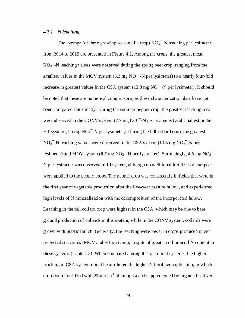
4.3 Results and discussion .......................................................................................... 90 4.3.1 Fresh vegetable yield .................................................................................... 90 4.3.2 N leaching ..................................................................................................... 91 4.3.3 Soil mineral N content .................................................................................. 92 4.3.4 N uptake relative to fertilization ................................................................... 93
VITA ............................................................................................................................... 129
vii
LIST OF TABLES Table 2.1 Initial soil conditions at study depths of three study agroecosystems. ............. 39
Table 2.2 Management characterization of three study agroecosystems, as characterized by cropping system duration, and tillage, nutrient and irrigation input intensities........... 40
Table 2.3 Crop timing and fertilizer rates in three study agroecosystems. Timing of the crop rotation is detailed by planting date (PD) to final termination date (TD) by primary tillage or crop removal. ..................................................................................................... 41
Table 2.4 Spearman rank correlation values for N2O flux and soil mineral nitrogen (NO3¯-N and NH4
+-N) and soil temperature, and carbon dioxide flux and soil temperature in three study vegetable production systems. ............................................... 42
Table 3.1 Measured soil bulk density (BD) and texture and calibrated saturated hydraulic conductivity (Ksat), saturation (θs), 1/3 bar (θ1/3), 15 bar (θ15) and residual (θr) soil water content ............................................................................................................................... 69
Table 3.2 Measured and simulated daily average temperature, R2 and RMSE values of soil temperature (ST) in Conventional (CONV), High Tunnel Organic (HT), and Low Input (LI) system during 2014-2016. ................................................................................ 70
Table 3.3 Measured and simulated average, R2 and RMSE values of volumetric soil water content in Conventional (CONV), High Tunnel Organic (HT), and Low Input (LI) system during 2014-2016. ............................................................................................................. 71
Table 3.4 Measured and simulated average, R2 and RMSE values of soil NO3¯-N content in Conventional (CONV), High Tunnel Organic (HT), and Low Input (LI) system during 2014-2016. ........................................................................................................................ 72
Table 3.5 Measured and simulated cumulative N2O-N flux during each crop period, R2
and RMSE values in Conventional (CONV), High Tunnel Organic (HT), and Low Input (LI) system during 2014-2016. ......................................................................................... 73
Table 3.6 Measured and simulated crop yield during the cropping season 2014-2016. ... 74
Table 3.7 Simulated soil N processes and loss pathways from 100 cm soil profile in three vegetable systems.............................................................................................................. 75
Table 4.1 Fertility and irrigation management for model crops in the five study systems............................................................................................................................................ 96
Table 4.2 Mean marketable (USDA grades 1&2) fresh yield of pepper, beet and collard from 2014, 2015 and 2016 in the five study systems. ...................................................... 98
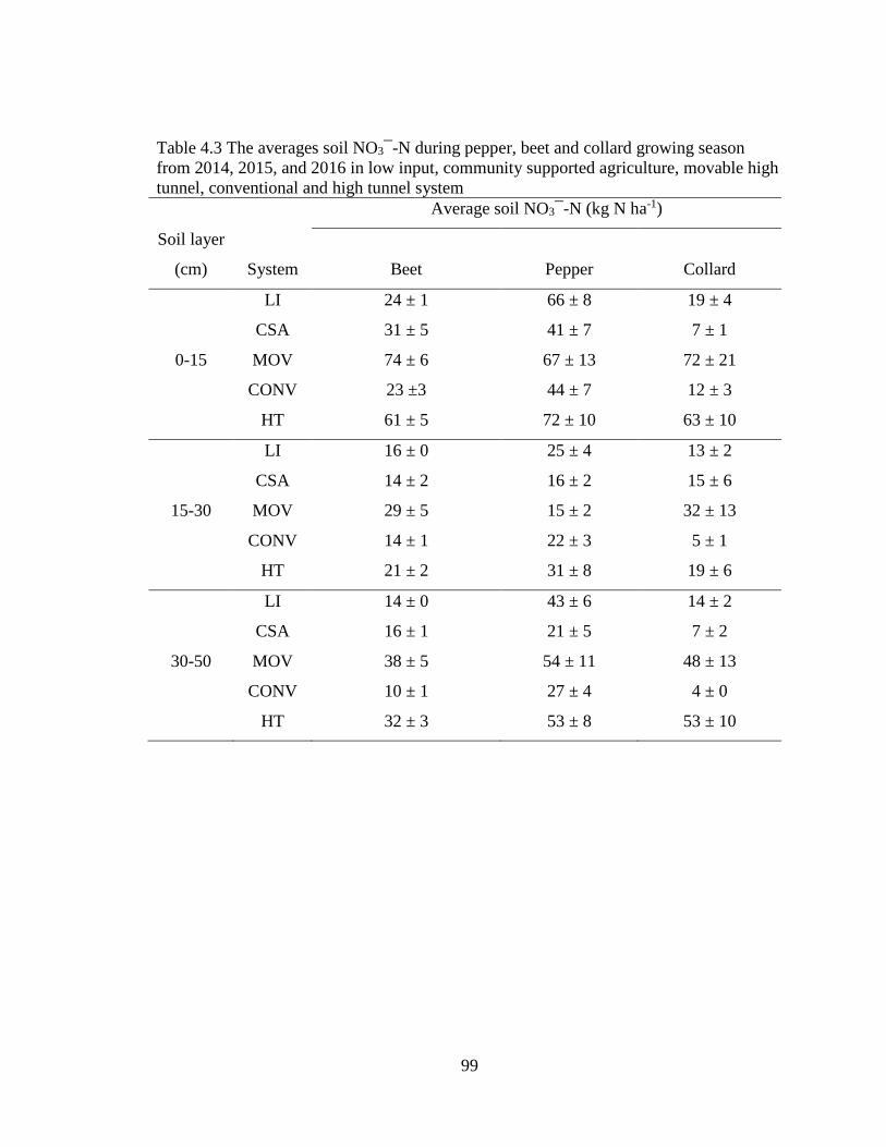
Table 4.3 The averages soil NO3¯-N during pepper, beet and collard growing season from 2014, 2015, and 2016 in low input, community supported agriculture, movable high tunnel, conventional and high tunnel system .................................................................... 99
Table 4.4 The Average crop N uptake and N fertilizer applied in five systems. ............ 100
viii
LIST OF FIGURES
Figure 2.1 Time series data from the Low Input (LI) system from 2014 – 2016, including CO2 and N2O flux, soil water content and precipitation, and soil NH4
+-N and NO3¯-N, total mineral N extracted from ion exchange resin bags, and leaching measured via ion exchange resin lysimeters. ................................................................................................ 43 Figure 2.2 Time series data from the Conventional (CONV) system from 2014 – 2016, including CO2 and N2O flux, soil water content and precipitation, and soil NH4
+-N and NO3¯-N, total mineral N extracted from ion exchange resin bags, and leaching measured via ion exchange resin lysimeters. .................................................................................... 44 Figure 2.3 Time series data from the High Input Organic (HT) system from 2014 – 2016, including CO2 and N2O flux, soil water content and precipitation, and soil NH4
+-N and NO3¯-N, total mineral N extracted from ion exchange resin bags, and leaching measured via ion exchange resin lysimeters. .................................................................................... 45 Figure 2.4 Systems-level comparison of (a) Cumulative greenhouse gas (GHG) emission, (b) Crop yield, (c) Yield-scaled global warming potential (GWP), and (d) Crop N uptake in the 2014-2016 crop rotation. ......................................................................................... 46 Figure 3.1 Measured and simulated soil water content at (a) 10 cm (b) 30 cm and (c) 50 cm and (d) soil temperature at 10 cm in Conventional System (CONV) during the year 2014-2016. ........................................................................................................................ 76 Figure 3.2 Measured and simulated soil water content at (a) 10 cm (b) 30 cm and (c) 50 cm and (d) soil temperature at 10 cm in High Tunnel Organic System (HT) during the year 2014-2016. ................................................................................................................ 77 Figure 3.3 Measured and simulated soil water content at (a) 10 cm (b) 30 cm and (c) 50 cm and (d) soil temperature at 10 cm in Low Input System (LI) during the year 2014-2016................................................................................................................................... 78 Figure 3.4 Measured and simulated soil NO3¯-N in layer (a) 0-15 cm (b) 15-30 cm (c) 30-50 cm and (d) N2O emission in the Conventional System (CONV) during the year 2014-2016. ........................................................................................................................ 79 Figure 3.5 Measured and simulated soil NO3¯-N in layer (a) 0-15 cm (b) 15-30 cm (c) 30-50 cm and (d) N2O emission in the High Tunnel Organic System (HT) during the year 2014-2016. ........................................................................................................................ 80 Figure 3.6 Measured and simulated soil NO3¯-N in layer (a) 0-15 cm (b) 15-30 cm (c) 30-50 cm and (d) N2O emission in Low Input System (LI) during the year 2014-2016. . 81 Figure 4.1 Overview of five model farming systems representing a gradient of intensification, as characterized by timing of production and fallow periods, tillage frequency, and nutrient inputs......................................................................................... 101 Figure 4.2 Mean NO3-N per lysimeter values in model crops in the five study systems from 2014, 2015 and 2016 .............................................................................................. 102
1
CHAPTER 1. INTRODUCTION
1.1 Sustainable intensification in vegetable systems
Meeting society’s growing need for food while minimizing harm to the natural
resource base upon which food production depends has been characterized as the
collective “grand challenge” for agriculture (Foley et al., 2011). There is broad
understanding that this challenge must be met largely on existing agricultural lands, and
through managing natural resources more efficiently than they are currently (FAO, 2011;
Tilman et al., 2011). Sustainable intensification invokes environmental goals such as
optimizing the use of external inputs (Matson et al., 1997; Pretty 1997, 2008), increasing
rates of internal nutrient recycling, decreasing nutrient loss (Gliessman, 2007), and
closing yield gaps (Mueller et al., 2012; Pradhan et al., 2015; Wezel et al., 2015). To
date, intensification efforts have focused largely on staple grain systems, but efforts to
sustainably intensify fruit and vegetable production systems are particularly timely due to
a suite of economic and environmental factors.
Similar to all sectors of crop and livestock production, global vegetable
production has increased substantially in the past 50 years, with rising population growth
and intensification of agricultural production systems (FAOSTAT, 2018). The five-fold
increase observed in global vegetable yields since 1961 is a function of both increasing
production area and increasing productivity on existing lands in production. This increase
is largely due to conversion of lands from staple grain production to high-value specialty
crops, particularly in small-holder farming areas experiencing declining grain prices
(Weinberger and Lumpkin, 2007). The dual trends of diversification into vegetable
production and intensifying production systems has been particularly strong in Asia,
2
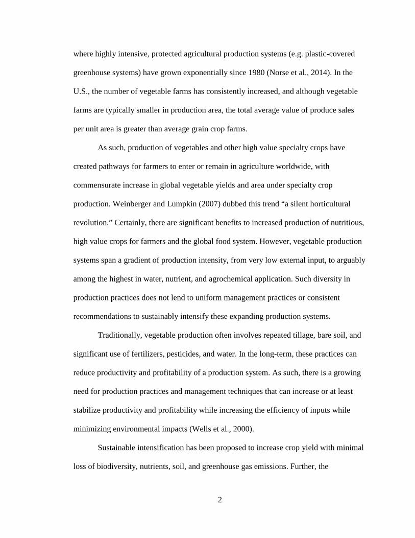
where highly intensive, protected agricultural production systems (e.g. plastic-covered
greenhouse systems) have grown exponentially since 1980 (Norse et al., 2014). In the
U.S., the number of vegetable farms has consistently increased, and although vegetable
farms are typically smaller in production area, the total average value of produce sales
per unit area is greater than average grain crop farms.
As such, production of vegetables and other high value specialty crops have
created pathways for farmers to enter or remain in agriculture worldwide, with
commensurate increase in global vegetable yields and area under specialty crop
production. Weinberger and Lumpkin (2007) dubbed this trend “a silent horticultural
revolution.” Certainly, there are significant benefits to increased production of nutritious,
high value crops for farmers and the global food system. However, vegetable production
systems span a gradient of production intensity, from very low external input, to arguably
among the highest in water, nutrient, and agrochemical application. Such diversity in
production practices does not lend to uniform management practices or consistent
recommendations to sustainably intensify these expanding production systems.
Traditionally, vegetable production often involves repeated tillage, bare soil, and
significant use of fertilizers, pesticides, and water. In the long-term, these practices can
reduce productivity and profitability of a production system. As such, there is a growing
need for production practices and management techniques that can increase or at least
stabilize productivity and profitability while increasing the efficiency of inputs while
minimizing environmental impacts (Wells et al., 2000).
Sustainable intensification has been proposed to increase crop yield with minimal
loss of biodiversity, nutrients, soil, and greenhouse gas emissions. Further, the
3
sustainability of the production systems should also be associated with temporal and
spatial stability of yield as it relates to changes key soil properties (Schrama et al., 2018).
Agricultural intensification and the resulting increases in yields have mainly been
attributed to intensive irrigation practices, agrochemical inputs and intensive tillage. Due
to problems of environmental degradation and perceived public health risk, there is
growing interest in alternative farming systems including organic (no synthetic fertilizer
and pesticide use) and low-input farming systems, which are being explored as ways to
improve overall soil health, agricultural sustainability, and environmental quality (Poudel
et al., 2002). However, more study of alternative production systems is needed to
understand how input use and production practices in these systems affect environmental
factors (Clark and Tilman, 2017). In the sections below, the literature regarding particular
aspects of agricultural intensification are reviewed, including nutrient and irrigation use,
use of fallow periods, and their effects on yield.
1.1.1 Fertilizers
Fertilizer use in vegetable crops is routine. For example, 98 percent of tomato
production area was fertilized in the US in 2010 at the rate of 160 kg N ha-1 (USDA
NASS, 2011). This is relatively high rate in comparison to other agricultural systems (e.g.
small grains, forages, etc.) in the U.S. However, it pales in comparison to excessive rates
applied in horticultural systems in input-intensive regions in the world. For example, N
fertilizer use has been documented to be as high as 1000 kg ha-1 in covered vegetable
areas of China (Zhu et al., 2005; Ju et al., 2007). Although increased N fertilization rates
within a certain range have been shown to directly correlate to increases in crop yields in
certain crop families (e.g. cole crops, Congreves et al., 2015), the effect of increased
4
fertilizer rates may be negated by the greater influence of climate (temperature and
precipitation) on crop yield. A recent study by Cui et al. (2018) demonstrated a 7.8-9.5
Mg ha-1 increase in grain yield with enhanced management practice, while at the same
time reducing N fertilizer application (kg N per unit area) by 8.5-15.6 %. Further, a 23-35
% decrease in reactive N losses (N2O emission, NH3 volatilization, NO3¯ leaching) and
19-29 % reduction in greenhouse gas emission were achieved (Cui et al., 2018). The
efficiency of fertilizer uptake by crop plants, particularly N fertilizers, and the
environmental fate of fertilizer losses vary by the nature of the fertilizer. Mineral N
fertilizer is commonly applied in mineral (inorganic) form as urea and solutions of urea
and ammonium nitrate, with urea being most readily volatilized as ammonia (Battye et
al., 1994). The use of “complete” fertilizer (containing N-P-K) is also common in
vegetable production (Blatt and McRae, 1988), with the N component of these fertilizers
generally consisting of urea and ammoniacal N.
In low-input and organic systems there is greater reliance on organic N sources,
such as manures, composts, and byproducts of animal and plant processing industries
(Gaskell and Smith, 2007). These are used in combination with crop rotations that often
include annual and perennial cover crops or forages. Internal N cycling in these systems
more closely mimic natural systems (Dawson et al., 2008). Compost, a source of plant
nutrients, is also commonly used in organic and conventional vegetable production
systems. In organic production systems, compost use is typically augmented with organic
fertilizers during peak production and late season at periods of peak crop N demand
(Gaskell and Smith, 2007). However, the uncertainty of nutrient content and availability
in these biological amendments can lead to over or under-fertilization, build up and
5
leaching of nutrients, or lack of synchrony between nutrient supply and plant uptake
(Drinkwater and Snapp, 2007). It is necessary to understand how organic inputs and their
management influence the temporal dynamics of soil inorganic N availability in the
context of the farming system to balance the essential soil functions of providing crop
fertility while reducing N losses to the environment (Norris and Congreves, 2018).
1.1.2 Irrigation
Vegetables are often irrigated. Surface and sub-surface drip irrigation has been
increasingly used to irrigate vegetable crops around the world. Relative to other methods
of irrigation such as flood, furrow or sprinkler irrigation systems, drip irrigation has
greater water use efficiency than other water application methods (Darwish et al., 2003).
Drip irrigation has been consistently shown to increase crop yield and water use
efficiency in vegetable production systems (e.g. Singadhupe et al., 2003; Yaghi et al.,
2013). Drip irrigation provides water directly to the plant root zone, and when coupled
with practices that supply water in small quantity but frequent application, generally
produces higher ratios of yield per unit area and yield per unit volume of water than
typical surface or sprinkler systems (Darwish et al., 2003). In rain-protected agriculture
systems, including high tunnels, all water is supplied via irrigation. Drip irrigation is the
recommended irrigation method in these systems. Although all crop water is supplied via
irrigation, the use of water is often reduced compared to irrigated open field production
due to evapotranspiration loss (Fernandez et al., 2007). Some of the greatest growth in
vegetable production systems has been in the use of such protected culture systems which
include the use of greenhouses and polyethylene tunnels (e.g. high tunnels, hoop houses)
in which vegetables are grown in-ground in a semi-controlled environment. Growth in
6
horticultural crops produced in protected culture rose by 44% from 2009 to 2014 (USDA
NASS, 2014). This pales in comparison to the adoption of protected agriculture in China,
which accounts for 90% of global greenhouse structures (Chang et al., 2013) through
rapid intensification of the agriculture sector since the 1980’s (Norse and Ju, 2015). Yield
in the protected agriculture can be twice as high as that over open culture (Chang et al.,
2013). High tunnels are also commonly used to produce high value crops. With proper
planning and management techniques, high tunnels can optimize yields, increase fruit
quality, and provide season extension opportunities for high-value vegetable crops
(O’Connell et al., 2012). Generally, high tunnels provide the opportunity for earlier crop
planting and earlier harvest compared to open field conditions. O’Connell et al. (2012)
reported similar yield in the first year and 33 % more tomato yield in the second year in
high tunnels compared to open field conditions.
1.1.3 Crop rotation and managed fallow periods
Crop rotation is a key strategy to control environmental stresses and improve crop
performance in conventional and organic vegetable systems. However, the need for
biological inputs to replace synthetic inputs, and an emphasis on soil organic matter
management in organic production drive organic growers to adopt major changes
compared to their conventional counterparts. Higher cover crop diversity, frequent cover
crop rotation, use of legume crops, and intercropping are more common in low input and
organic farming. The increased complexity and diversity of crop rotations are likely to
provide strong environmental benefits and enhanced ecosystem services (Barbieri et al.,
2017), although more study of how the elements of rotation, tillage, cover crop use, and
fertilizers/amendments interact is needed.
7
Cover crops, such as annual grasses or legumes, are often included between
vegetable crops to prevent erosion, provide organic matter and nutrients for subsequent
crops and minimize leaching (Thorup-Kristensen et al., 2003; Robacer et al., 2016).
Although cover crops are not able to provide enough total N for a high N-demanding
vegetable crop, or mineralize in synchrony with plant N demand (Drinkwater and Snapp,
2007) they may still increase the net economic returns (Muramoto et al., 2011) by
trapping N otherwise lost. In temperate regions, cool season cover crops are most
common, and are planted in the late summer or early fall, after harvest of warm season
vegetables. They are terminated in the subsequent spring prior to planting. They may also
be used in other temporal windows in the rotation vegetable systems. For example short-
season summer cover crops provide weed suppression and nutrients for fall-planted
vegetable crops (Creamer and Baldwin, 2000).
The interaction between cover crops (managed fallow) and the subsequent crop
fertility regime affects the nature and magnitude of nutrient input losses in
agroecosystems. Shelton et al. (2018) quantified N loss via leaching, NH3 volatilization,
N2O emissions, and N retention in plant and soil pools of corn agroecosystems in
Kentucky. Cover crop species and fertilization schemes affect N loss and availability in
corn systems and dominant N loss pathways varied by season. NO3¯-N leaching was the
primary loss pathway during the cover crop growing season, especially in treatments
using leguminous monocultures (hairy vetch only), while N loss via N2O-N and NH3-N
emissions was dominant during the corn growing season. Nitrogen contribution of
legume-grass cover crop mixture into fertilizer application rates may reduce N loss
without sacrificing yield (Han et al., 2017).
8
Pasture-crop rotations, which utilize a multiple year period of grazed pasture
fallow followed by crop production, are popular in Argentina, Brazil, and Uruguay
(Garcia-Prechac et al., 2004) and have significant effects on soil properties. Soil
aggregate stability increases quickly by including pasture in the rotation with crops, due
to the combination of a) the absence of tillage operation during the pasture cycle; (b) the
dense and fibrous grass root systems that promote aggregation (Haynes et al., 1991). The
combined use of cropping and pasture in rotation results in reduced soil erosion
compared to continuous cropping (Garcia-Prechac et al., 2004). Agricultural soils benefit
from the re-introducing perennial grasses and legumes into the crop field by gaining
organic matter and strengthening their capacity for long-term productivity and
environmental resiliency (Franzluebers et al., 2014). Crop-pasture rotation systems, as
reported by Franzluebbers et al. (2014) exist in the US in some integrated livestock and
crop production systems. Perennial forages in pasture add organic matter to soil, provide
soil C sequestration, improve nutrient cycling, and support biological diversity.
1.1.4 Effect of intensification on yields
Intensification packages such as drip irrigation and plastic mulch have been
generally found to increase crop yield while increasing water use efficiency. Singadhupe
et al. (2003) reported 3.7-12.5% increases in tomato fruit yield, 31-37% water savings,
and 8-11% increase in N uptake by plants by using drip irrigation system in tomato crops.
Similar results have been found in potato (Zhang et al., 2017), and a suite of other crops.
Intensification packages in vegetable systems can involve significant nutrient, water,
plastic, and pesticide inputs. The net effects of these efforts have increased yields and
decreased labor, improved nutrient and water use (Steffaneli et al., 2010), and reduced N
9
losses to the environment, even when viewed relative to other intensified production
systems, such as row crop agriculture systems (Goulding, 2000). Yield improvements
through careful and efficient management of crop nutrients and water, precision farming,
less intensive tillage could reduce future greenhouse gas emissions rather than clearing
the lands for crop production (Burney et al., 2010).
The effects of intensification on crop yields has also been framed in the context of
farm management philosophies or certifications. Specifically, organic and conventional
systems have been compared as proxies for low and high intensity systems, respectively
(e.g. Seufert et al., 2012). Examining the effect of these systems-level comparisons has
been the subject of several recent meta-analyses of yield and ecosystems services in these
systems. Relative yield stability (i.e., yield stability per unit yield produced) was higher
in conventionally managed fields by 15% compared to organically managed fields
(Knapp and van der Heijden, 2018). However, compared to conventional agriculture,
organic agriculture generally had a positive effect on a range of environmental benefits,
including above and belowground biodiversity, soil carbon stocks and soil quality.
Similarly, de Ponti et al. (2012) reported 20% lower yield in organic systems compared to
conventional systems. However, the difference in crop yield between organic systems
and conventional systems were highly site specific; such as, in rain-fed legumes and
perennials on weakly acidic to weakly alkaline soil, the yield difference was below 5 %
(Seufert et al., 2012; Kniss et al., 2016). Kniss et al. (2016) also concluded that organic to
conventional yield ratios vary widely among crops. In an analysis of organic yield data
collected from over 10,000 organic farmers representing nearly 800,000 hectares of
organic farmland in the United States, their results demonstrated that the organic yield
10
average for all crops was 80% of conventional yield. Yield of organically produced cereal
crops maize and barley was 65% and 76% of conventional yield, respectively. Organic
squash, snap bean, sweet maize, and peach yields were not statistically different from
conventional yields. Despite consistency in the literature indicating that crop yields in
organic production are generally lower than conventional production, a meta-analysis of a
global dataset by Crowder and Reganold (2015) suggested the price premiums for
organic products may offset the lower yield with respect to net economic returns.
Recent meta-analyses (Garbach et al., 2016; Ponisio et al., 2015) identified
organic systems as exemplars of systems that frequently experience significant gaps in
actualized yield relative to potential yield (yield gaps). In these systems, relatively minor
increases in inputs and subtle modifications of management practices can offer the
potential of substantial yield increases, if these practices correct critically limiting
production factors (Foley et al., 2011). Such yield gaps are most pronounced in low-input
organic systems, attributed to the relatively low N concentration in biologically-based
amendments. However, correcting yield gaps in organic systems in ways that minimize
environmental impact may not strictly be a function of increasing inputs. Organic
vegetable production may include very intensive practices, such as year-round cropping
with lack of fallow periods, heavy irrigation and fertilization, and the use of protected
agriculture systems such as plastic covered greenhouses or high tunnels. The
simplification of these systems as binary components masks the diverse management
practices and input intensity within any given system, be they organic or conventional.
Vegetable production systems are highly diversified, and the soil plant water
balance, nutrient uptake and variability between vegetable crops within a system and
11
among the production systems have been poorly addressed (Gary et al., 1998). The
mechanisms and interaction of biotic and abiotic factors driving nutrient losses in
vegetable production systems have yet to be fully elucidated. With this general framing
of sustainable intensification in vegetable production systems in mind, this dissertation
focuses on the N dynamics related to intensification in diversified vegetable production
systems. In the sections below, the literature on N cycling in these systems from
empirical studies and simulation modeling literature is reviewed.
1.2 Nitrogen dynamics in vegetable cropping systems
1.2.1 N cycling and retention
The N cycle in agroecosystems includes assimilation, mineralization,
Table 2.2 Management characterization of three study agroecosystems, as characterized by cropping system duration, and tillage, nutrient and irrigation input intensities. Agricultural System
Cash Crop Production (typical months/year)
Tillage Frequency (approx. depth in m)
Nutrient Input Regime
Irrigation Method
Low Input Organic (LI)
8-9 Semi-annual soil preparation with primary inversion tillage (0.30 m), Secondary soil preparation with disc (0.20 m). In-season weed control via sweep cultivation (0.15 m).
Five-year fallow prior to cropping cycle, annual cool-season cover crop between cash crops.
Drip irrigation in plasticulture beds applied at the time of planting. Bare ground crops depended only on precipitation.
Conventional (CONV)
8-9 Semi-annual soil preparation with a soil spader (historically inversion tillage, 30 cm), secondary soil preparation with disc (0.20 m). In season weed control via sweep cultivation (0.10 m).
Annual cool-season cover crop between cash crops, Synthetic fertilizer applied pre-plant and split-application via fertigation in long-season crops.
Drip-irrigated.
Organic High Tunnel (HT)
12 Quarterly secondary tillage with rototiller (0.20 m). In season weed control via surface cultivation (0.05 m) with hand tools.
Table 2.3 Crop timing and fertilizer rates in three study agroecosystems. Timing of the crop rotation is detailed by planting date (PD) to final termination date (TD) by primary tillage or crop removal. Crop Rotation 2014 2015-2016 2016 System
Sweet pepper (Capsicum annum L., ‘Aristotle’)
Head lettuce (Letuca sativa, ‘Dov’)
Table beets (Beta Vulgaris, ‘Red Ace’)
Collards (Brassica oleracea var. medullosa, ‘Champion’)
Beans (Phaseolus vulgaris, ‘Provider’)
Low Input Organic (LI) PD to TD 14 May – 9 Sept -- 8 June – 3 Sept 11 Oct – 23 March 28 May – 4 Aug
Conventional (CONV)
PD to TD 20 May – 1 Aug -- 24 April – 7 Aug 19 Aug – 26 Feb 7 May – 26 July
Fertilizer
78 kg N ha-1 at planting on 20 May; split application of 9 kg N ha-1 on 29 May, 8 June, 16 June, 20 June, 27 June, 9 July
-- 56 kg N ha-1 at planting on 24 April
56 kg N ha-1 at planting on 19 Aug; split application of 9 kg N ha-1 on 8 Sept, 15 Sept, 22 Sept, 28 Sept, 2 Oct
56 kg N ha-1 at planting on 16 May
Organic High Tunnel (HT)
PD to TD 22 April – 29 July 15 Sept – 21 Nov 12 March – 12 June 25 Sept – 26 Feb 28 April – 8 July
Fertilizer
Horse manure compost equiv. to 24 ton ha-1, 45 kg N ha-1 of pelleted organic fertilizer (5-4-3) at planting
Same as for Sweet pepper
Same as for Sweet pepper
Same as for Sweet pepper
Same as for Sweet pepper
42
Table 2.4 Spearman rank correlation values for N2O flux and soil mineral nitrogen (NO3¯-N and NH4
+-N) and soil temperature, and carbon dioxide flux and soil temperature in three study vegetable production systems.
Environmental Variables
N2O
Low Input Organic Conventional High Tunnel
Soil mineral N
(0-15 cm) r = 0.30 r = 0.08 r = 0.20
Soil mineral N
(15-30 cm) r = 0.14 r = 0.02 r = 0.32
Soil mineral N
(30-50 cm) r = 0.28 r = 0.12 r = 0.13
CO2 r = 0.46 r = 0.26 r = 0.16
Soil temperature
(⁰C, 10 cm)
r = 0.35 r = 0.07 r = 0.15
CO2
r = 0.80 r = 0.55 r = 0.55
43
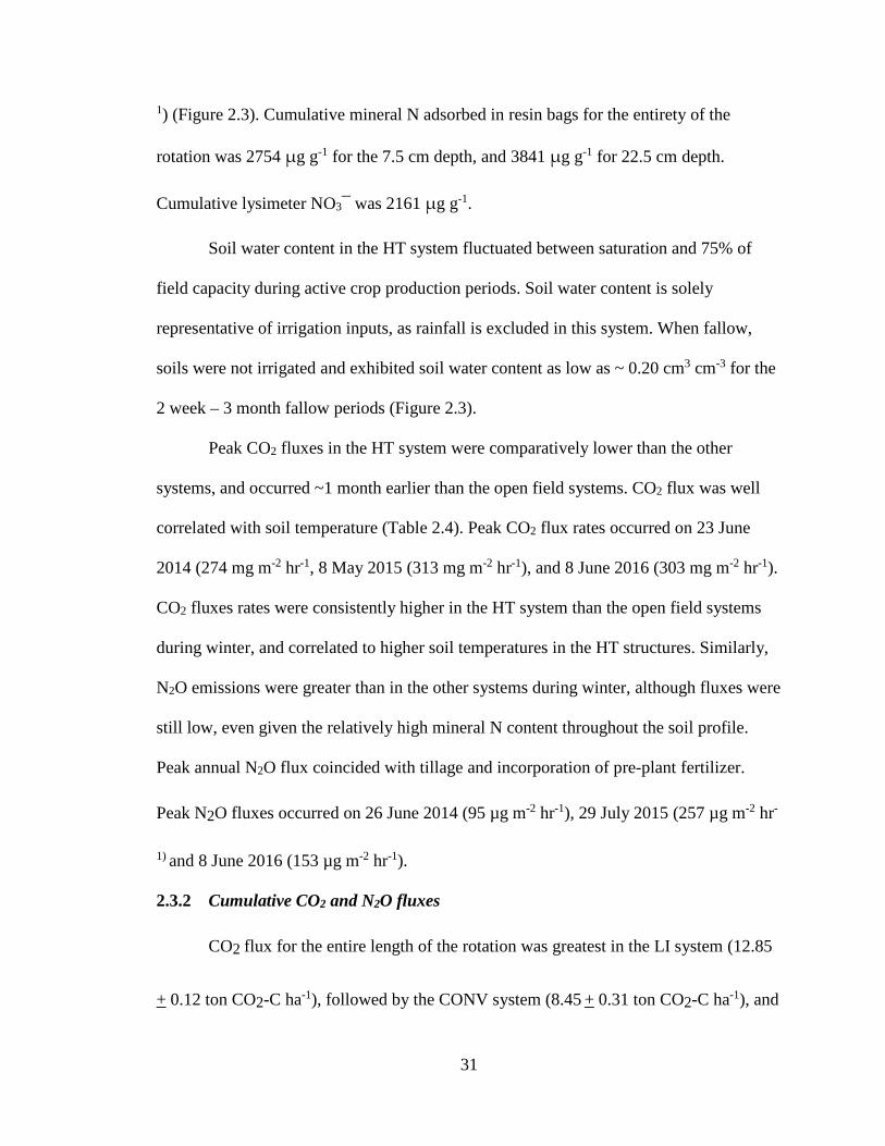
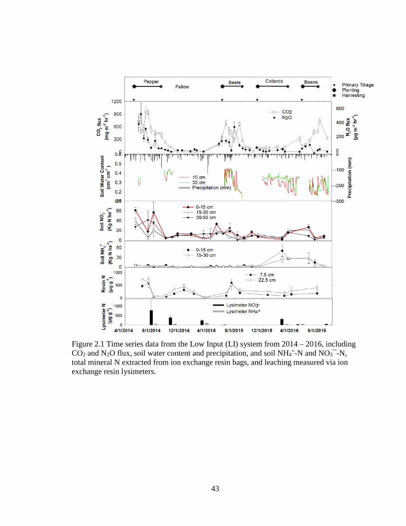
Figure 2.1 Time series data from the Low Input (LI) system from 2014 – 2016, including CO2 and N2O flux, soil water content and precipitation, and soil NH4
+-N and NO3¯-N, total mineral N extracted from ion exchange resin bags, and leaching measured via ion exchange resin lysimeters.
44
Figure 2.2 Time series data from the Conventional (CONV) system from 2014 – 2016, including CO2 and N2O flux, soil water content and precipitation, and soil NH4
+-N and NO3¯-N, total mineral N extracted from ion exchange resin bags, and leaching measured via ion exchange resin lysimeters.
45
Figure 2.3 Time series data from the High Input Organic (HT) system from 2014 – 2016, including CO2 and N2O flux, soil water content and precipitation, and soil NH4
+-N and NO3¯-N, total mineral N extracted from ion exchange resin bags, and leaching measured via ion exchange resin lysimeters.
46
*Yield Scaled GWP of LI beets (7.2 ±0.6) not included in graph for better view.
Figure 2.4 Systems-level comparison of (a) Cumulative greenhouse gas (GHG) emission, (b) Crop yield, (c) Yield-scaled global warming potential (GWP), and (d) Crop N uptake in the 2014-2016 crop rotation.
47
CHAPTER 3. USING RZWQM2 TO SIMULATE NITROGEN DYNAMICS AND NITROUS OXIDE EMISSIONS IN VEGETABLE PRODUDUCTION SYSTEMS
3.1 Introduction
Vegetable production area has increased consistently in the U.S, from 1949 to
2014 (USDA NASS, 2014). Although production area is expanding, the body of literature
on the effect of vegetable production on soil processes, greenhouse gas emissions, and
nutrient leaching is limited (Zhang et al., 2018). This is due, in part, to highly variable
production practices due to variability in crop choice, input and management intensity,
and the adoption of diverse conservation practices (Rezaei Rashti et al., 2015). Inorganic
fertilizers, cover crops, manure, and compost are sources of N, necessary for crop
production. However, increased N application significantly contributes to air and water
pollution and global warming (Galloway et al., 2004).
Agricultural soils contribute approximately 60% to total anthropogenic emissions
of N2O (Lokupitiya and Paustian, 2006), a potent greenhouse gas with global warming
potential 298 times greater than CO2 (IPCC, 2014). Primary source of N pollution to
groundwater and water bodies is from agricultural soils applied with N fertilizers (Tilman
et al., 2011). Although smaller in production area relative to staple grain crops, vegetable
production systems are often fertilized with higher rate of N fertilizer (Rosenstock and
Tomich, 2016) and most often irrigated. These inputs are likely driving the increased
N2O emissions and NO3¯ leaching losses that have been reported from vegetable
production systems (Liptzin and Dahlgren, 2016; Xu et al., 2016).
High temporal and spatial variability of fluxes in gases such as N2O fluxes (Fang
et al., 2015) makes it difficult to quantify emissions across variable agricultural
48
production systems. Further, process-based models allow an opportunity to simulate soil
N and C dynamics (Ma et al., 2012), predict N2O emissions (Fang et al., 2015) and crop
production (Jiang et al., 2019; Uzoma et al., 2015). However, the majority of process-
based models have been developed for grain crop and pasture-based systems, and many
do not incorporate production methods and technologies common in vegetable
production.
For example, the use of plastic mulches is one of the components of intensive
production of vegetable crops, which continues to grow worldwide (Lament, 1993). Drip
irrigation in conjunction with plastic mulch reduces evaporation from mulched soil and
decreases irrigation requirements. Drip irrigation has been increasingly used to irrigate
vegetable crops globally and reported to have greater water use efficiency compared to
flood, furrow or sprinkler irrigation methods (Darwish et al., 2003). Vegetable production
in protected agriculture systems, in which covered structures exclude rainfall are also
increasingly common world-wide. In the US, the use of high tunnels, which are passively
heated and ventilated structures with crops grown in-ground production is also increasing
(USDA NASS, 2014). These semi-controlled environments are protected from rainfall
and typically have higher temperatures than the open field, allowing for extension of the
growing season of warm season crops and production throughout the winter season in
many temperate climates. However, these temperature and moisture regimes differ
substantially from the open field. In such protected structures, as with many of the
vegetable production technologies and practices mentioned above affect soil temperature
and soil water dynamics, which are major drivers of soil N dynamics and other
agroecosystem processes. Many of these technologies and production practices are
49
difficult to simulate in process-based models developed for open field grain or forage
systems.
Root Zone Water Quality Model 2 (RZWQM2) is a comprehensive ecosystem model
that simulates soil water, temperature, N and C dynamics and crop yield (Ahuja et al.,
2000). RZWQM2 has been extensively applied to better understand soil water, soil N and
C dynamics, N leaching, and crop yield in agronomic crop production systems such as
corn, wheat, and soybean (Ma et al., 2007; Malone et al., 2007; Yu et al., 2006).
RZWQM2 has not been widely used in vegetable production systems, save a notable
exception by Cameira et al. (2014), who used the model to study water and N budgets for
organically and conventionally managed urban vegetable gardens. However, recent
additions to the model by Fang et al. (2014) incorporated the Simultaneous Heat and
Water (SHAW) (Flerchinger and Saxton, 1989) model in to RZWQM. The updated
RZWQM2 can be used to simulate soil water and temperature under plastic mulch, a
common vegetable production technique. Drip irrigation is also supported by the model,
as are a number of vegetable crops, making RZWQM2 an ideal candidate for evaluating
for its ability to simulate a wide variety of vegetable production systems.
RZWQM2 require detailed input data for weather, soil physical, chemical and
hydraulic information, and agronomic management to run the model (Malone et al.,
2004; Gillette et al., 2018). Provided with this information and appropriately calibrated
and validated, RZWQM has been used widely to simulate NO3¯ leaching (Yu et al., 2006;
Gillette et al., 2018; Jiang et al., 2019). Further, Fang et al. (2015) combined the nitrous
oxide emission (NOE) model and DAYCENT model and incorporated them into
RZWQM to simulate N2O emissions, and then it has been used to simulate N2O emission
50
by other researchers (Gillette et al., 2017, 2018; Jiang et al., 2019). As such, RZWQM2 is
a strong process-based model to help researchers better understand the soil water, N
dynamics and N leaching across the complex array of crop management, fertilizer use,
crop rotation, and tillage frequency characteristic of vegetable production systems. The
objective of this study was to simulate soil water, N2O emission, soil NO3¯-N processes,
and crop yield in diversified vegetable rotations that include a variety of common
vegetable production practices.
3.2 Materials and methods
3.2.1 Research sites
This three-year rotational study was initiated in early spring 2014 in two sites in
central Kentucky with Maury silt loam soil (a fine, mixed, active, mesic Typic
Paleudalfs). Each system contained six replicate plots. Details about research sites for this
chapter was utilized from previous chapter. Initial soil conditions for each system are
listed in Table 2.1.
3.2.2 Cropping systems description
The three vegetable production systems utilized in this study were characterized
by fallow periods, tillage intensity, and irrigation and nutrient inputs. They are presented
in Table 2.3. Additional management and input descriptions are provided in Shrestha et
al. (2018). The Conventional system (CONV) consisted of a winter wheat (Triticum
aestivum L.) cover crop during winter 2014, planted in late fall and terminated with
tillage in early spring (Table 2.3), followed by vegetables.
The Organic High Tunnel system (HT) consisted of three, replicated unheated 9.1
m x 22 m greenhouse structures. Horse manure compost and granular organic fertilizer
51
(Harmony 5-4-3, BioSystems, LLC, Blacksburg, VA) were incorporated into soil at a rate
of 67 kg N ha-1 before planting each crop. Details about amount and timing of fertilizer
application are presented in Table 2.3. All crops were drip irrigated.
The Low Input Organic system (LI) consisted of a long-term rotation of a five-
year mixed grass/legume pasture followed by a three-year rotation of annual crops. No
supplemental fertilizer was added, and drip irrigation was used exclusively for pepper.
Irrigation was applied only if precipitation was insufficient at critical stages of crop
development. Both the HT and LI systems were certified organic under the US National
Organic Program Guidelines (USDA, 2018).
3.2.3 Measured data
Soil, plant and N2O flux sampling methods are presented in detail in Shrestha et
al. (2018). Briefly, soils were sampled monthly at 0-15 cm, 15-30, and 30-50 cm depths
for mineral N (NH4+ and NO3¯) from six replicate plots. On each sampling date, three
cores were taken per plot at each depth, homogenized, and bulked for a single analysis
per plot. N2O flux was sampled bi-weekly (excluding periods when the ground was
frozen) using a FTIR-based field gas analyzer (Gasmet DX4040, Gasmet Technologies
Oy, Helsinki, Finland). The static chamber method (Parkin and Venterea, 2010) was
used, with rectangular stainless-steel chambers (16.4 cm x 52.7 cm x 15.2 cm) installed in
each plot. Gas fluxes were calculated by using the following equation (Iqbal, 2013):
(𝐹𝐹) = 𝛥𝛥𝛥𝛥𝛥𝛥𝛥𝛥
𝑉𝑉𝐴𝐴
𝜌𝜌
Where F is the gas flux rate (mg m−2 h−1), ΔC/Δt indicates the increase/decrease
of gas concentration (C) in the chamber over time (t), V is the chamber volume (m3), A is
the chamber cross-sectional surface area (m2), 𝜌𝜌 denotes the gas density at 25°C.
52
Cumulative gas fluxes were estimated by interpolating trapezoidal integration of flux
versus time between sampling dates and calculating the area under the curve (Venterea et
al., 2011).
Soil water potential was measured using granular matrix (Watermark) sensors
(Irrometer Co., Riverside, CA) installed at three depths in the soil profile (10, 30, and 50
cm depths), with one sensor per depth, for a total of three per plot. Watermark sensor data
was transmitted continuously via wireless transmitters to a data logger (Watermark
Monitor 900M, Irrometer, Co., Riverside, CA), with readings logged each time when the
water potential changed. Soil temperature was measured at the time of N2O flux
measurement with digital soil thermometer inserting at of 10 cm depth from soil surface.
Fresh vegetable yields were measured from the entire plot area of 13.5 m2 from
each of the plots. Pepper fruits, collard leaves and green beans were harvested at multiple
times as the harvestable portion reached marketable stage, and table beets were harvested
once, as roots reached marketable size. Plant C and N content were analyzed from a
subsample plant material collected from each plot at the final biomass harvest. Final
biomass samples were dried at 60 ⁰C until a constant mass was achieved, homogenized
on a Wiley Mill (Thomas Scientific, Swedesboro, NJ), and a subsample ground on a
roller mill (C.Z-22072, U.S. Stoneware, East Palestine, OH). One plant sample from each
plot for each crop was analyzed for percent C and N on an elemental analyzer (Thermo
Scientific FlashSmart, CE Elantech, Lakewood, NJ).
3.2.4 Model description
RZWQM2 is a one-dimensional agricultural system model, which simulates
mineralization and immobilization of crop residues, mineralization of soil N,
53
volatilization, nitrification, and denitrification (Ahuja et al, 2000). Soil water content,
nutrient leaching and crop yield are also simulated. The agricultural management input
options are crop and crop cultivar selection, planting date, manure and fertilizer
application, tillage, irrigation and pesticide application (Ma et al., 2012). Brooks–Corey
equations are used to relate volumetric soil water content (θ) and soil suction head (h)
(Ma et al., 2012). The potential evaporation and crop transpiration are described by the
Shuttle-Wallace equation. Fang et al. (2014) incorporated the simultaneous Heat and
Water (SHAW) (Flerchinger and Saxton, 1989) model into RZWQM (Ahuja et al., 2000),
and used to simulate surface energy balance and canopy temperature along with crop
growth and production in different climate and cropping seasons. RZ-SHAW model was
able to quantify the effect of crop growth on the energy balance under different
agronomic management practices. RZWQM2 provides soil water content, root
distribution, soil evaporation, soil transpiration, leaf area index, and plant height at each
time step to SHAW and then SHAW provides soil ice content, updated soil water content
due to ice and freezing, and soil temperature to RZWQM (Fang et al., 2014). RZWQM2
provides soil evaporation (AE), which is used by SHAW to compute the energy balance
of the surface soil layer by forcing water vapor flux from the soil surface, and therefore
latent heat flux, to equal the soil evaporation (Fang et al., 2014). Soil heat flow and
temperature in the soil matrix, considering convective heat transfer by liquid and latent
heat transfer by vapor for freezing soil is given by
54
where Cs and T are volumetric heat capacity (J kg-1 K-1) and temperature (°C) of the soil,
ρi is density of ice (kg m-3), θi is volumetric ice content (m3m-3), Kt(s) is soil thermal
conductivity (W m-1K-1), ρl is density of water, cl is specific heat capacity of water (J kg-1
K-1), θi is liquid water flux (m s-1), qv is water vapor flux (kg m-2 s-1), Lf is latent heat of
fusion (335,000 J kg-1) and ρv is vapor density (kg m-3) within the soil (Fang et al., 2014).
The N2O emission algorithm in RZWQM2, as described in Fang et al. (2015), was
partly taken from the DAYCENT model (Parton et al., 1998; Del Grosso et al., 2000) and
Nitrous Oxide Emission (NOE) model (Henault et al., 2005). N2O emission from
nitrification (N2O_nit) is calculated as following (Del Grosso et al., 2000) and presented
below:
where FrN2O-Nit is the fraction of nitrification for N2O emissions, and 0.02 was used as the
default value in DAYCENT (Del Grosso et al., 2000; Parton et al., 2001); FSWnit is the
soil water factor for the oxygen availability effect on N2O emission during nitrification
(Khalil et al., 2004) taken from the NOE model.
N2O emission from denitrification (N2Oden) is calculated as following (Del Grosso et al.,
2000):
N2Oden=FrN2O-den × Rden
FrN2O-den=1
1+RNO-N2O+RNO-N2O
N2Onit=FrN2O-nit × FSWnit R
nit
FSW_nit=0.4 WFPS -1.04
WFPS+1.04
55
where FrN2O-den is the fraction of denitrification for N2O emissions; RNO- N2O is the ratio of
NO to N2O; RN2-N2O is the ratio of N2 to N2O; [NO3] is soil NO3¯-N; D is gas diffusivity
in soil (Davidson and Trumbore, 1995); WFPS is water filled pore space.
3.2.5 Model input, calibration and validation
Weather input data for the CONV and LI systems, including daily minimum and
maximum air temperature, wind speed and direction, shortwave radiation and relative
humidity were entered as daily summary data local to the research sites (KYMESONET,
2018). Daily precipitation data for LI was taken from a Georgetown-Scott County
Regional Airport, Scott county (8 km from research site) downloaded from NOAA
(NOAA, 2018). For the HT system, daily maximum, minimum temperature and relative
humidity values were summarized from data loggers measuring on 15-minute intervals,
mounted 2 m high in the center of the structures (WatchDog B102, Spectrum
Technologies, Aurora, IL). The calculation of daily solar radiation inside tunnels was
taken from VegSyst V2 model (Gallardo et al., 2016) and calculated as the product of
solar radiation outside and tunnel plastic roof transmissivity:
SRin = SRout x τ
RNO-N2O=4+9 tan-1{0.75π (10 D-1.86)}
π
RN2-N2O= max {0.16 k1, k1 exp (-0.8 [NO3]
[CO2])} max (0.1, 0.015 WFPS 100-0.320)
k1= max (1.5, 358.4-350 D)
56
τ for double layer polyethylene sheet for high tunnel = 0.7 (Biernbaum, 2013)
where SRin is the incoming solar radiation, SRout is the outgoing solar radiation, and τ is
the transmissivity of polyethylene sheet cover on high tunnel. RZ-SHAW model was
used for pepper in 2014 in all three system and only in CONV collard, as these crops
were grown under black plastic mulch (Plastic emissivity - 0.95, albedo - 0.05 and
transmissivity - 0.86), RZWQM2 was used for the other crops.
Model simulations were done for each crop separately. For pepper, the model was
started on April 1st, 2014 and ended on 10th September 2014 in all systems. Final soil C,
N pools from the pepper were used to initialize the model for the following crops. Model
simulation for cover crop in CONV, lettuce in HT and fallow in the LI system was started
on 11th September 2014. Starting date for model run for beet, collard and bean were 1st
March 2015, 16th August 2015 and 1st March 2016 in all systems. The cumulative N2O
emissions were calculated for each crop season separately. Soil bulk density was
measured from field samples (Table 3.1), while soil texture data and soil water content at
1/3 and 15 bar of soil (Table 3.1) were obtained from USDA NRCS Web soil survey
(Web Soil Survey, 2018), and calibrated in CONV system (Table 3.1). Saturated
hydraulic conductivity, soil water content at 1/3 bar and 15 bar for the 50 cm depth were
calibrated in relation to the measured soil water content in the CONV system; and then
followed by calibration at 30 cm and 10 cm soil depth. Initial values for fast and slow
residue pools; slow, medium and fast soil humus pools; and microbial pools were
calculated based on measured soil carbon data (Table 3.1) by conducting a “warm up”
run (to get stable soil residue and microbial pool) for 10 years under current weather and
management practices for the CONV and HT system. Initial carbon pool for the LI
57
system were obtained by running the grass module to mimic the pasture production
system (Feng et al., 2015). Model default values were used for soil chemistry data. Crop
parameters were calibrated with the measured yield component data from CONV system
and validated by HT and LI system. For the pepper crop, the crop parameters were
obtained from DSSAT pepper variety ‘Capistrano’, as plant height, leaf structure and
fruit type were similar to pepper variety ‘Aristotle’. For bean, dry bean variety ‘Andean
Habit 1’ was chosen, as plant characteristics were close to variety ‘Provider’. For the
table beet, the DSSAT sugar beet var ‘SVRR1142E’ was chosen and we modified the
crop parameters G2 leaf expansion rate during stage 3 to 130 cm2 cm-2 day-1, G3 Root
tuber growth rate to 14.5 g m-2 day-1 and plant biomass at half of maximum height to 9.07
g plant-1 (Tei et al., 1996). The DSSAT cabbage variety ‘990001 Tastie 4’parameter was
modified to simulate the collard crop. The specific leaf area of cultivar under standard
growth conditions (SLAVR) was modified to 80 cm2 g-1 (Uzun and Kar, 2004) and
maximum size of full leaf (three leaves) (SIZLF) was measured, 350 cm2. The HT system
included an additional crop in the rotation, due to the year-round production capacity of
the system. The DSSAT cabbage crop parameters; SLAVR modified to 100 cm2 g-1 (Tei
et al., 1996) and SIZLF modified to 250 cm2, as measured to simulate a lettuce crop. The
model performance in simulating the soil water, soil NO3¯, N2O emissions and crop
biomass was evaluated by root mean square error (RMSE) and coefficient of
determination (R2).
58
3.3 Results and discussion
3.3.1 Soil temperature
RZWQM2 simulated soil temperature was compared with the measured values
(Table 3.2). In all cropping systems, RZWQM2 underestimated the soil temperature for
all crops except for peppers, which were grown under black plastic mulch. In the CONV
system, RZWQM2 underestimated average soil temperature (Figure 3.1 (d)) by 3, 2.3, 0.2
and 1.5 °C during the cover crop, beet, collard and bean growing seasons, respectively. In
the HT system, RZWQM2 underestimated average soil temperature by 7.6, 3.6, 3.8 and
2.5 °C during lettuce, beet, collard and bean growing season, and shown in Figure 3.2(d).
Similarly, the average soil temperatures were underestimated by 4.3, 0.9, 4.4 and 3.3 °C
during fallow, beet, collard and bean growing seasons, respectively in LI system. The
underestimation might be related to timing of temperature measurement; as soil
temperatures were measured during the day time, while the model simulated the
temperature values as an average of daily temperature (Jiang et al., 2019). The R2 and
RMSE values ranged from 0.43-0.86 and 1.22-3.68 °C in CONV; 0.63-0.86 and 1.26-
3.15 °C in HT; 0.24-0.93 and 1.93-3.55 °C in LI system (Table 3.2).
3.3.2 Soil water content
The simulated soil water content in three different layers (15 cm, 30 cm and 50
cm) were evaluated using measured values for CONV, HT and LI systems (Table 3.3).
The simulated water contents in different soil layers showed reasonably good agreement
with measured soil water (Table 3.3). The model overestimated the soil water content
values at 10 cm and 30 cm during pepper and collard green growing season in all systems
and values were close to the measured value at the layer 50 cm. It should be noted that
59
pepper and collard were grown in a raised bed, while other crops were grown in a flat
bed. In the CONV system, RZWQM2 was able to simulate soil water well during pepper,
and beet growing seasons, but collard and bean were not well simulated at 30 cm depth
(Figure 3.1). RZWQM2 was able to simulate soil water content well in the HT system
except for the collard growing season (Figure 3.2), where the R2 values were lower than
0.33 for all soil layers. RZWQM2 was able to simulate the soil water in the LI system
well (Figure 3.3), as R2 values are more than 0.65 in all cases except for bean growing
season (Table 3.3). The lower agreement between the simulated and measured soil water
values in the CONV and LI systems might be related to additional water uptake by
weeds, which were neither simulated nor measured. R2 values may be lower during the
overwinter grown collard in the CONV and HT systems, as the soil water sensors used
tend to record lower soil water content values during freezing soil conditions.
3.3.3 Soil nitrate content
The simulated soil NO3¯-N content in three different layers (0-15 cm, 15-30 cm
and 30-50 cm) were compared using measured values for CONV, HT, and LI systems
(Table 3.4). During the pepper growing season, RZWQM2 underestimated the soil NO3¯-
N content in all systems in all three soil layers. In the CONV system, the model was able
to simulate soil NO3¯-N well during the cover crop, beet and bean growing seasons
(Figure 3.4(a), 3.4(b), 3.4(c)), showing the R2 values ranging from 0.38 to 0.97 (Table
3.4). However, there was not good agreement between simulated values and the
measured values during pepper and collard growing season in the CONV system. It
should be noted that the pepper and collard in the CONV system were grown under black
plastic mulch in an approximately 15 cm high raised beds spaced ~ 1m apart, with the
60
field consisting of a series of such plastic-covered raised beds. Initial fertilizer was
broadcast evenly over the field prior to raising the beds. However, subsequent fertilizer
was applied with drip irrigation during the growing season, which narrowed the fertilizer
application to the soil water pattern dispersed by the drip irrigation. The model simulated
soil NO3¯-N well during the cover crop, beet, and bean portion of the rotation, where the
crops were planted in flat bed and the row-to-row distance was small (Table 3.4). The
largest difference between RZWQM2 simulated and field measured soil NO3¯-N values
were in CONV pepper, a system in which the standard best management practice in the
growing region is to split the fertilizer application between pre-plant and in-season
fertigation. In this practice, 2/3 of the fertilizer is applied during the growing season
weekly (though this may be more frequent) at a commercially-recommended rate. The
measured values were taken from samples within the middle 50% of the bed, which may
have a greater concentration of NO3¯-N than the edges of the bed. From our results, we
could say that the model simulated soil NO3¯-N well in beet and bean in all systems,
which were grown in flat bed conditions and in which the row to row distances were
lower than pepper and collard.
In the HT system, soil NO3¯-N values in the 0-15 cm layer were poorly simulated
throughout the rotation (Figure 3.5a), with R2 values below 0.29 (Table 3.4). This might
be attributed to the high denitrification N loss and N immobilization, despite high
simulated mineralization (Table 3.7). However, the model was able to simulate the soil
NO3¯-N reasonably well at 15-30 cm soil layer (Figure 3.5b). The model did not do well
(R2 < 0.03) in simulating soil NO3¯-N content in the 30-50 cm layer during pepper,
lettuce and beans growing season. The inability of the RZWQM2 model to simulate the
61
soil NO3¯-N content in the upper 15 cm of soil in the high tunnel grown vegetable system
might be associated with the source of fertilizer used, tillage intensity, soil temperature
and moisture regime. In the HT system, only organic fertilizer and horse manure compost
were used to fertilize the vegetable crops in all cropping seasons. A small tiller which
turns over only the top 10 cm of soil, was used; concurrently, almost all fertilizer applied
to crops remains in the top 10 cm. As some researchers reported, N decomposition,
denitrification, and nitrification processes are not straightforward in organic manure
applied soil (Chen et al., 2013), and resulted in differences in timing and the amount of
simulated and observed soil NO3¯-N under high tunnels. RZWQM2 simulated results
showed continuous N mineralization and denitrification process during the fallow period
in HT system, that simulated loss (the major contribution being from denitrification), and
resulted in decreased simulated soil NO3¯-N concentration present in soil during fallow
period. Cassman and Munns (1980) reported that there is significant interactive effect of
soil water and temperature on N mineralization. Sharp decline in net N mineralization
occurs between 0.3 and 2-bar and thereafter it decreases gradually over the 2- to 10-bar
range at all temperatures (Cassman and Munns, 1980). Reduced soil microbial activity
could be expected in fallow periods without irrigation in the high tunnels (Knewtson et
al., 2012), which are protected from rainfall, and are only irrigated during the crop
growing period. Despite having higher soil temperature in the tunnel, a driver of
microbial activities in soil, is overridden by the reduced organic decomposition when
moisture is a limiting factor (Knewtson et al., 2012). Nitrate leaching was also
significantly reduced from greenhouse grown vegetables in elevated temperature
62
conditions, which led to higher NO3¯ concentrations in greenhouse condition than in
open field conditions.
In the LI system, simulated soil NO3¯-N values in the surface layer (0-15 cm)
were not in good agreement with the observed values throughout the rotation, with R2
values below 0.10 and RMSE values ranging between 4.59 to 31.82 kg ha-1 during crop
growing seasons (Table 3.4). However, the simulated 15-30 cm soil NO3¯-N content
were in good agreement with the measured values, except for the bean growing season.
The simulated soil NO3¯-N content values at 30-50 cm depth were in excellent agreement
with the measured values showing the R2 values more than 0.70 for all crops except
collard (R2 = 0.18) and pepper and, RMSE values ranging between 2.09 – 4.24 kg ha-1
(Table 3.4).
3.3.4 Nitrous oxide emissions
The measured and simulated cumulative N2O-N emissions during each cropping
season in CONV, HT and LI system are presented in Table 3.5 and daily N2O fluxes are
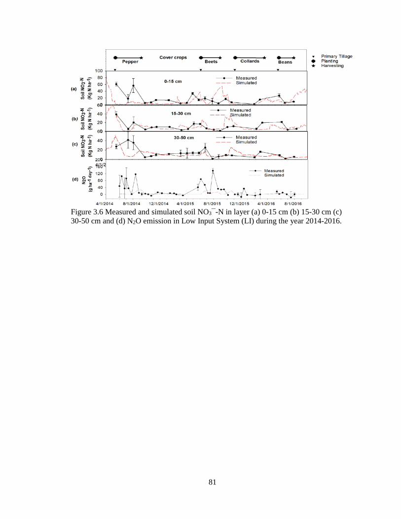
shown in Figure 3.4(d) for CONV, Figure 3.5(d) for HT and Figure 3.6(d) for LI system.
In the CONV system, RZWQM2 simulated the cumulative N2O-N emission well from
2014 to 2016, while the model generally overestimated fluxes in HT system and
underestimated fluxes in LI system the total N2O-N emission throughout the crop
rotation.
In the CONV system, observed cumulative N2O-N emissions were 0.25, 0.29,
1.10, 0.25, and 0.93 kg N2O-N ha-1 during pepper, cover crop, beet, collard and bean
growing season, while the simulated N2O-N emissions were 0.74,0.10, 0.67, 0.62 and
0.68 0.96 kg N2O-N ha-1 during pepper, cover crop, beet, collard and bean growing
63
season (Table 3.5). For the CONV system, RZWQM2 reliably simulated the N2O
emissions, showing the R2 values 0.36 to 0.78 except for cover crop and RMSE values
between 0.90 to 6.83 g N2O-N ha-1 day-1. RZWQM2 overestimated the emission during
the pepper and collard growing season while underestimating emission during cover crop,
beet and bean growing season. It should be noted that the pepper and collard were grown
under plastic mulch. The model was able to reliably simulate the peaks of N2O emission
in the CONV system (Figure 3.4(d)) but simulated higher fluxes than measured just after
the tillage and incorporation of fertilizer after pepper planting. The better simulation of
magnitude and timing of soil NO3¯-N and N2O fluxes in the CONV system might be
related to the source of N, and the spatial pattern of synthetic N fertilizer application.
Fang et al. (2015) and Gillette et al. (2017) also reported good agreement between
RZWQM2 simulated and measured N2O emissions from synthetic N fertilizer field
with/without tillage. In the CONV system, the overestimation of N2O during the pepper
(which were grown under plastic mulch) growing season might be related to the
overestimation of soil temperature. Kim et al. (2014) also reported greater simulated N2O
emissions than measured values with radish grown under plastic mulch and fertilized
with 50-150 kg N ha-1.
In the HT system, the measured cumulative N2O-N emissions were 0.59, 0.39,
0.69, 1.20 and 1.59 kg N2O-N ha-1, whereas simulated values were 2.11,0.45, 0.71, 1.42
and 3.03 kg N2O-N ha-1, during the pepper, cover crop, beet, collard and bean growing
season (Table 3.5). In the HT systems, RZWQM2 simulated cumulative N2O-N
emissions were close to measured values during the lettuce, beet and collard growing
season, but overestimated the cumulative N2O-N emission during the pepper and bean
64
portions of the rotation. This overestimation of the N2O-N emission in high tunnels might
be related to the simulation of higher peaks just after fertilizer application. In general,
simulations underestimated the soil NO3¯-N content but overestimated soil N2O
emissions. There are various practices that may not be well simulated in RZWQM2 that
contribute to this discrepancy. First, high tunnels are structures that exclude rainfall from
the growing environment. As such, water for crops was provided exclusively by
irrigation; soil temperature and moisture dynamics vary from the open field conditions in
which the model was developed and is typically used. Irrigation inputs were applied via
drip irrigation, as discussed above. Finally, this system utilized compost applications
prior to crop planting, which may mineralize at rates greater than predicted in the
simulation. The net effects of these discrepancies resulted in a variation in timing of
denitrification and nitrification and other N processes between simulated and observed
conditions in high tunnels. These issues are demonstrated in simulation results such as
those shown in Figure 3.5(d), which show N2O peaks on August 11th, 2014 and August
20th, 2015, that were larger than the measured values, and which contributed largely to
the cumulative fluxes in the HT system. RZWQM2 simulated higher N2O emissions in
the HT system, but lower N2O emissions in the HT were observed in our work. Most of
the literatures showed that N2O fluxes increased exponentially with increasing soil
moisture, temperature and NO3¯ content and decreases with reduced soil moisture
content (Dobbie et al., 1999). The algorithms for N2O emission, adopted by Fang et al.
(2015) to incorporate into RZWQM2 model, are based on soil water content, soil
temperature, and soil N content. The interactive effect of changed temperature and soil
moisture content on N2O emissions varies with different agro-ecosystems with different
65
agricultural management. Decreased N2O emissions indicated might be attributed to an
overriding effect of dry soil moisture conditions on N2O emissions in N-fertilized
vegetable soil even though enough soil N substrate was present (Xu et al., 2016). Warmer
and drier conditions, as in high tunnels, could affect both the population abundance and
community structure of nitrifiers and denitrifiers in the vegetable soil (Xu et al., 2016).
In the LI system (Table 3.5), the measured N2O-N emissions were 2.73, 0.13,
1.38, 0.98 and 0.39 kg N2O-N ha-1, whereas the RZWQM2 simulated values were 0.36,
0.12, 0.22, 0.41 and 0.14 kg N2O-N ha-1 during the pepper, cover crop, beet, collard and
bean growing seasons, respectively (Table 3.5). RZWQM2 underestimated the
cumulative N2O-N emission for all crop in the LI system. The plots in the LI system were
converted from rotational grazing pasture into crop fields to grow vegetable in 2014. At
the start of the crop in 2014, we observed large peaks of N2O flux but that decreased in
subsequent years. The model could not simulate the large peaks at the starting of the
planting season in 2014. The first month after pepper planting was the major contributor
to the overall observed emission in LI system, which contributed 25 % of observed
cumulative emission during entire cropping period from 2014 to 2016. Pinto et al. (2004)
reported high N2O flux after tillage operations followed by rapid reduction in perennial
grasslands. The RZWQM2 model estimated the N2O emission based on the existing soil
N content and the soil water content. The role of crop residue on N2O emission is
complex and is not taken into account by RZWQM2. The addition of the crop residue not
only supply the N for N2O production, it also enhanced oxygen depletion by stimulating
microbial respiration and promoted anaerobic conditions for denitrification and N2O
production (Chen et al., 2013). In a laboratory study by Kravchenko et al. (2017),
66
gravimetric soil water content of the plant residue (separated from soil-residue mixture)
exceeded gravimetric soil water content of soil from soil residue mixture by a factor of 4-
10, accelerated N2O emission. Deng et al. (2013) reported the significantly increased N2O
emission from soil from vegetable production systems after addition of the organic
matter. In LI, the simulated N2O emissions were lower than the measured values. The
simulated N leaching from LI vegetables were higher than from the other two systems.
The major simulated N leaching loss in LI systems were contributed by the fallow period
and the collard growing period. Elevated N leaching was reported by Evanylo et al.
(2008) during winter when soil is without an actively growing crop and precipitation
exceeds evaporation. Simulation results also showed the 60 and 74 kg ha-1 of mineralized
N during the fallow period and collard in LI system. The higher N leaching from the crop
field converted from pasture might be attributed to underestimating mineralized N from
residues and higher infiltration rate (Evanylo et al., 2008).
3.3.5 Crop yield and biomass
The measured and simulated crop yield on dry matter basis in CONV, HT and LI
systems are shown in Table 3.6. RZWQM2 was reliably able to estimate the pepper, beet
and bean yield in all systems. Collard yield were overestimated, as we did not sample
total plant biomass at each green leaf harvesting, rather only harvestable yield, whereas
the model included all the leaves on the plant. Measured beet yields were low due to
weed pressure in LI system. Collard yields were low due to low seasonal temperatures
during the collard growing season, which was expected and is well simulated by
RZWQM2. Green bean yields were overestimated by RZWQM2 in the LI system
67
compared to the measured yield, which may be due to model not accounting for N uptake
by weeds during bean growing season.
3.3.6 Model simulated outputs through the soil profile
The simulated soil N mineralization, immobilization as well as denitrification,
runoff, seepage and emission losses of N from the 100 cm soil profile from each crop
growing season from CONV, HT and LI system are presented in Table 3.7. In LI system,
The N simulated seepage losses were higher during the fallow period and crop growth
failure during beets (due to weed pressure) and collards (due to very low temperature
during early growth). This shows the lack of growth of plant not only results in loss of
crop yield, but also leads to the losses of N from the field.
3.4 Conclusion
RZWQM2 was selected for this purpose due to recent modifications to
accommodate vegetable production and for its widespread use in simulating soil N and C
processes, and provision to simulate soil water and temperature under plastic mulch. Our
results suggest that RZWQM2 may effectively simulate soil temperature, soil water and
N dynamics and vegetable yields grown for crops grown on bare ground (e.g. beet,
collard and bean). RZWQM2 underestimated the soil temperature for all crops except for
pepper, which were grown under black plastic mulch. RZWQM2 simulated soil NO3¯-N
content reasonably well during beet, collard and bean growing seasons in CONV and LI
systems, but could not simulate well during pepper crops which were grown under plastic
mulch. RZWQM2 simulated cumulative N2O emission from 2014 to 2016 reasonably
well compared to field measured values in the CONV system, while the model
overestimated it in the HT system and underestimated it in the LI system. Crop yields
68
were simulated well in all systems. RZWQM2 simulated soil water content well in
CONV, HT, and LI vegetable systems. Although vegetable systems are very complex in
terms of the crop use, fertilizer use, crop rotation, tillage frequency, the use of a well
calibrated model helps researchers better understand the soil N dynamics and leaching.
69
3.5 Tables and figures
Table 3.1 Measured soil bulk density (BD) and texture and calibrated saturated hydraulic conductivity (Ksat), saturation (θs), 1/3 bar (θ1/3), 15 bar (θ15) and residual (θr) soil water content
Uncalibrated Calibrated
Soil depth (cm)
BD Sand Silt Clay Ksat θ1/3 θ15
Ksat θ1/3 θ15 θs θr
(g cm-3) % % % cm hr-1 (cm3 cm-3) cm hr-1 (cm3 cm-3) (cm3 cm-3)
Table 3.2 Measured and simulated daily average temperature, R2 and RMSE values of soil temperature (ST) in Conventional (CONV), High Tunnel Organic (HT), and Low Input (LI) system during 2014-2016.
Table 3.3 Measured and simulated average, R2 and RMSE values of volumetric soil water content in Conventional (CONV), High Tunnel Organic (HT), and Low Input (LI) system during 2014-2016.
10 cm 30 cm 50 cm
Cropping system Crops Mes Sim RMSE R2 Mes Sim RMSE R2 Mes Sim RMSE R2
Table 3.4 Measured and simulated average, R2 and RMSE values of soil NO3¯-N content in Conventional (CONV), High Tunnel Organic (HT), and Low Input (LI) system during 2014-2016. Cropping System 0-15 cm 15-30 cm 30-50 cm Crops Mes Sim RMSE R2 Mes Sim RMSE R2 Mes Sim RMSE R2 kg N ha-1 kg N ha-1 kg N ha-1 Pepper 107 13 89.19 0.34 67 10 37.50 0.54 76 10 43.13 0.27
Figure 3.1 Measured and simulated soil water content at (a) 10 cm (b) 30 cm and (c) 50 cm and (d) soil temperature at 10 cm in Conventional System (CONV) during the year 2014-2016.
77
Figure 3.2 Measured and simulated soil water content at (a) 10 cm (b) 30 cm and (c) 50 cm and (d) soil temperature at 10 cm in High Tunnel Organic System (HT) during the year 2014-2016.
78
Figure 3.3 Measured and simulated soil water content at (a) 10 cm (b) 30 cm and (c) 50 cm and (d) soil temperature at 10 cm in Low Input System (LI) during the year 2014-2016.
79
Figure 3.4 Measured and simulated soil NO3¯-N in layer (a) 0-15 cm (b) 15-30 cm (c) 30-50 cm and (d) N2O emission in the Conventional System (CONV) during the year 2014-2016.
80
Figure 3.5 Measured and simulated soil NO3¯-N in layer (a) 0-15 cm (b) 15-30 cm (c) 30-50 cm and (d) N2O emission in the High Tunnel Organic System (HT) during the year 2014-2016.
81
Figure 3.6 Measured and simulated soil NO3¯-N in layer (a) 0-15 cm (b) 15-30 cm (c) 30-50 cm and (d) N2O emission in Low Input System (LI) during the year 2014-2016.
82
CHAPTER 4. CHARACTERIZING THE SUSTAINABILITY OF INTENSIFICATION IN VEGETABLE SYSTEMS
4.1 Introduction
Sustainable intensification, and related concepts, are increasingly being advocated
as frameworks to reconcile needs for increasing agricultural yields with maintaining
environmental integrity (Wezel et al., 2015). Agricultural input efficiency (AIE) has been
proposed as a holistic metric to evaluate agriculture’s environmental impact relative to
yields (e.g. Robertson and Swinton, 2005; Clark and Tilman, 2017). Measured as the
amount of food produced per unit of input, AIE has utility in evaluating the point at
which when additional inputs do not equate to additional yields, and subsequently are
linked to impacts on the environment (Clark and Tilman, 2017). AIE has been used as a
unifying concept for discussions linking input:output efficiencies to the broader impacts
of agriculture on the environment, including energy use, land use, nutrient impact on
waterways, and greenhouse gas emissions (Clark and Tilman, 2017). Among these,
nitrogen (N) losses from agricultural systems to the environment have been considered
the most problematic (e.g. Robertson and Swinton, 2005). The nitrogen use efficiency
(NUE) of a cropping system can be increased by achieving greater N uptake efficiency
from applied N and reducing the amount of N lost from soil organic and inorganic N
pools (Cassman et al., 2002).
Sustainable agriculture-oriented vegetable production systems, whether managed
according to an environmentally-minded certification (e.g. USDA organic, etc.) or
utilizing conservation-minded best practices are managed with explicit intention to
minimize environmental impact while optimizing yields. However, evaluating NUE, and
AIE more generally in such alternative systems is lacking (Clark and Tilman, 2017).
83
Historically system comparisons have been binary, pitting conventional vs. organic (e.g.
Seufert et al., 2012), or greenhouse vs. open field (Clark and Tilman, 2017). However,
specific production practices related to the intensity of production systems are highly
variable, even among sustainable and organic vegetable production systems.
A finer-scale understanding of how organic inputs and their management in the context
of the farming system influences the temporal dynamics of soil inorganic N availability is
needed to balance the essential soil functions of providing crop fertility while reducing N
losses to the environment (Norris and Congreves, 2018).This work aims to characterize
AIE, specifically NUE and the N dynamics driving uptake and losses, across a gradient of
sustainable vegetable production systems utilized in the mid-southern region of the US.
Intensification in these systems is characterized by fertilization, water use, tillage, and
use of fallow periods. Such data offer the opportunity to evaluate the “trade-offs”
between specific environmental impacts and yield, utilizing model crops produced in the
spring, summer, and fall.
4.2 Materials and methods
Three model crops, representing typical crops grown seasonally in the region, were
studied for three years in each of five production systems, beginning in early spring, 2014
(Table 4.1). The five systems spanned two sites in central Kentucky with Maury silt loam
soil (a fine, mixed, active, mesic Typic Paleudalfs); 1) The University of Kentucky
Horticulture Research Farm (UK HRF) in Lexington, KY (37°58'29"N, 84°32'05"W); 2)
a local organic farm in Scott County, Kentucky (38°13'20"N, 84°30'38"W). Both farms
are in the central Bluegrass region of Kentucky, with similar rainfall, temperature, and
soil type (annual precipitation of 1209, 1475 and 1011 mm; average air temperature of 12
84
ºC, 13.3 ºC and 14.2 ºC in 2014, 2015 and 2016, respectively). Each system contained
three replicate plots measuring 9 m x 0.75m.
4.2.1 Cropping systems
The five vegetable production systems were selected to represent a gradient of
intensification, as characterized by duration of fallow periods, tillage intensity, irrigation,
and fertilization (Figure 4.1). General management aspects of each of these systems are
described below.
4.2.1.1 Low input system (LI)
The LI system is based on an 8-year rotation consisting of a five-year period of
mixed grass/legume pasture that is rotationally grazed or cut for hay for grass-finished
beef and calf production. After the five-year fallow period, the pasture was broken with
deep inversion plowing, disking and surface rototilling to transition fields into a three-
year rotation of annual crops. No supplemental fertilizer was added, and drip irrigation
was provided only for the pepper crop. Crops produced on bare ground received only
natural rainfall and no supplemental irrigation. Tillage and fertilizer for model crops are
detailed in Table 4.1. For the past 15 years, the farm has grown diversified organic
vegetables in the annual crop portion of the rotation, after transitioning from two
generations of conventional tobacco production in a similar rotation. This system is
representative of a low external input commercial organic vegetable farming system, and
is a working partner farm marketing a diversity of organic vegetable crops and animal
products through local market channels.
85
4.2.1.2 Community supported agriculture system (CSA)
The CSA system is characterized by the seasonal production of vegetable crops
with inclusion of cover crops once per year in rotation. The rotation involves production
of over 40 different vegetable crops, grown in a rotation based on alternation of botanical
families. Vegetable crops were supplied with 25 ton ha-1 compost one time per year, in
the Fall, typically followed by a cool season (Winter) cover crop. A granular, manure-
based organic fertilizer (Nature Safe 10-2-8, Darling Ingredients, Irvine, TX) applied at
the time of planting to bring the crop fertility to the commercial production recommended
fertilizer rate (UK Cooperative Extension Service, 2014) using a nutrient budget
approach which accounts for roughly for the nutrient contribution of the compost
additions and legume cover crop. All crops were irrigated with sub-surface drip
irrigation. All crops were drip irrigated in every 2-3 days interval in summer and 3-4 days
interval in winter season depending on rainfall. Annual primary tillage using a rotary
spader (Imants, ImantsUSA, Perkiomenville, PA) was used to incorporate cover crop
residue and prepare fields, followed by frequent shallow cultivation utilizing ground-
driven rolling basket weeders or finger weeders for weed control. Tillage and fertilization
for model crops are detailed in Table 4.1. This system is representative of a medium-
scale, input- and mechanization-intensive commercial organic vegetable farming
operation utilizing best management practices for open-field organic production. This is a
working demonstration and education farm on the UK Horticulture Research Farm site,
marketing a diversity of organic vegetable crops primarily through a community
supported agriculture program.
86
4.2.1.3 Movable high tunnel system (MOV)
Movable high tunnels are full size (9.1 m x 22 m) passive solar greenhouses made
of steel framing with a polyethylene film coating that are moved once per year (see High
Tunnel system for additional description). MOV structures were rotated through a series
of three positions such that crops are grown under the cover of the structure for one year
continuously, then the structures were moved, and cropped area is planted into legume
and cereal cover crops for two years. After 2 years, tunnels moved back to previous place
to grow organic vegetable crops. In the MOV system, 24 ton ha-1 horse manure compost
and 45 kg N ha-1 of pelleted organic fertilizer (Harmony 5-4-3, BioSystems, LLC,
Blacksburg, VA) were applied in to soil before planting each crop. Irrigation in the MOV
system was via drip irrigation, as the plastic cover over the structure excluded all rainfall.
All crops were drip irrigated in every 2-3 days interval in summer and 3-4 days interval
in winter season. Tillage and fertilization for model crops are detailed in Table 4.1. This
system is representative of an alternative production system for organic high tunnel
production focused on maintaining soil health and reducing disease incidence in these
typically production-intensive systems.
4.2.1.4 Conventional system (CONV)
The CONV system consisted of a winter wheat (Triticum aestivum) cover crop
terminated by mowing and tillage in early spring utilizing a rotary spader, followed by
seasonal annual vegetable production. Fertilization included complete, balanced mineral
fertilizers (Miller 19-19-19, Miller Chemical and Fertilizer, Hanover, PA) applied pre-
plant and in-season, split-application of calcium nitrate fertilizer (13-0-0, PureCal, Master
Plant-Prod Inc., Brampton, ON) via fertigation when required for the crop as per
87
commercial vegetable production recommendations for the study region (UK
Cooperative Extension Service, 2014). All crops were drip irrigated in every 2-3 days
interval in summer and 3-4 days interval in winter season depending on rainfall. Tillage
and fertilization for model crops are detailed in Table 4.1. This system is representative
of an input-intensive conventional vegetable production system utilizing best
management practices.
4.2.1.5 High tunnel system (HT)
The HT consisted of three, replicated static unheated 9.1 m x 22 m steel structures
with polyethylene film covering. As is typical for management of these structures, crops
are grown in soil without supplemental heat or light, and are only passively ventilated
through manual opening of doors and side curtains. High tunnel systems are “season
extending” technologies used in specialty crop production, allowing for lengthening the
growing season of warm-season crops by approximately one month each in the spring
and fall, and allowing for production of cool-season vegetables throughout the winter in
the study region. Also typical to these systems, cover crops were not used, as these
intensive production systems often are used to produce of high value crops at times when
market premiums are captured through early or late season production. As such, fallow
periods are not considered economically efficient unless they address a production issue,
such as pathogen or pest management. All crop residues were removed from the system
to minimize pathogen presence. In the HT system, 24 ton ha-1 horse manure compost
(Wet mass) and 45 kg N ha-1 of pelleted organic fertilizer (Harmony 5-4-3, BioSystems,
LLC, Blacksburg, VA) was applied to soil before planting each crop. Supplemental
fertigation with liquid organic fertilizer (Brown’s Fish Fertilizer 2-3-1, C.R. Brown
88
Enterprises, Andrews, NC) was applied in-season only to the sweet pepper crop, at
flowering and heavy fruit set (twice total) at the recommended rate constituting an
additional 28 kg N ha-1 at each fertigation event. Irrigation in the HT system was via drip
irrigation, as the plastic cover over the structure excluded all rainfall. All crops were drip
irrigated in every 2-3 days interval in summer and 3-4 days interval in winter season.
Tillage and fertilizer inputs for model crops are detailed in Table 4.1. The system is
representative of year-round, organic high tunnel production systems that are input- and
production-intensive.
4.2.2 Model crops and management
Model crops were selected based upon crops that would be representative of
production practices in each model system (Table 4.1). As this project takes a systems
approach, timing of production varies slightly between systems, particularly between the
open field systems (LI, CSA and CONV) and the protected agriculture systems (MOV
and HT). Model crops were selected representing spring, summer, and fall production;
and collard greens (Brassica oleracea L. var. medullosa, ‘Champion’), respectively.
Three plots measuring 13.5 m2 each were randomly assigned within crop rows in each of
the systems. Rows were located in fields consisting of diversified vegetables in the LI
and CSA systems, with adjacent rows in plants of the same botanical family and/or
management regime. Fields in the CONV system were monocultures of the model crop.
Rows in the HT and MOV systems were within diversified tunnel systems consisting of
varies of crops being grown for season extension purposes. Model crops were in different
fields/rows each year, following the rotation scheme representative of each system.
89
4.2.3 Soil sampling
Soils were sampled monthly at 0-15, 15-30, and 30-50 cm depths for mineral N
(NH4+ and NO3¯). On each sampling date, three cores were taken per plot at each depth,
homogenized, and bulked for a single analysis per plot. Fresh soil samples were kept
refrigerated (~ 4.4⁰ C) until processing, passed through a 2 mm sieve and processed
within 24 h of sampling. Soil mineral N was extracted from a 5 g subsample of fresh soil
in 20 ml of 1M KCl (Rice et al., 1984) and analyzed via microplate spectrophotometer
(Epoch, BioTek Instruments, Inc., Winooski, VT), after NO3¯ was reduced using a
cadmium reduction device (ParaTechs Co., Lexington, KY) (Crutchfield and Grove,
2011). Nitrate leaching was assessed using ion exchange resin (IER) lysimeters placed
below the plant rooting zone (50 cm depth). IER lysimeters were constructed from PVC
tubing after the method of Susfalk and Johnson (2002), using 2 teaspoonfuls of resin per
lysimeter. IER lysimeters were replaced every three months, and once recovered,
disassembled, with resin mineral N extracted using 100 ml of 2M KCl in the method as
described above.
4.2.4 Yield and plant biomass sampling
Fresh vegetable yields for each system were measured from the entire plot area
from each plot. Yields represent marketable yield for each system, which includes all
direct market quality yields for the LI and CSA systems, and combined USDA grade 1
and 2 for each crop in the MOV, HT and CONV systems. Sweet pepper fruit, collard
leaves and beans were harvested at multiple times as the harvestable portion reached
marketable stage, and table beets were harvested once, as roots reached marketable size.
Plant biomass samples were collected from 2, 0.25 m2 samples per plot at the end of the
90
growing season, dried at 60⁰ C until a constant mass was achieved. Dried samples were
homogenized on a Wiley Mill and a subsample ground on a jar mill (U.S. Stoneware,
East Palestine, OH). Crop plant samples were analyzed for C and N content via elemental
analysis (Flash EA 1112, CE Elantech Inc., Lakewood, CA).
4.3 Results and discussion
4.3.1 Fresh vegetable yield
The average fresh beet, pepper fruit and collard leaves yield from 2014 to 2016 in
all five systems are presented in Table 4.2. Yields were consistently higher in the MOV
system, and lowest in the LI system across all crops. The movable tunnels were moved
every year, so the crops in the MOV system benefitted from the additional N supply by
the cover crops compared to the HT system. CSA and CONV yields were not markedly
different for any crop. Beet yields may have been low in the LI system due to low stand
density, or poor germination due to lack of irrigation, compared to the other study
systems, as well as higher weed pressure. Pepper yields may have been depressed in the
LI system due to weed pressure as well. Collard greens were also consistently planted
later in the LI system than in other systems, as is typical for the management of this
production system. In this system, management preference is for extensive production
with minimal input per unit area, with overall farm yields buffered by large cropping
areas and great crop diversity to buffer low yields or a crop failure. Overall, high tunnel
yields were greater due to improved crop quality grown under the protective structures, as
well as higher planting density common in these systems.
91
4.3.2 N leaching
The average (of three growing season of a crop) NO3¯-N leaching per lysimeter
from 2014 to 2015 are presented in Figure 4.2. Among the crops, the greatest mean
NO3¯-N leaching values were observed during the spring beet crop, ranging from the
smallest values in the MOV system (3.3 mg NO3¯-N per lysimeter) to a nearly four-fold
increase in greatest values in the CSA system (12.8 mg NO3¯-N per lysimeter). It should
be noted that these are numerical comparisons, as these characterization data have not
been compared statistically. During the summer pepper crop, the greatest leaching loss
were observed in the CONV system (7.7 mg NO3¯-N per lysimeter) and smallest in the
HT system (1.5 mg NO3¯-N per lysimeter). During the fall collard crop, the greatest
NO3¯-N leaching values were observed in the CSA system (10.5 mg NO3¯-N per
lysimeter) and MOV system (6.7 mg NO3¯-N per lysimeter). Surprisingly, 4.5 mg NO3¯-
N per lysimeter was observed in LI system, although no additional fertilizer or compost
were applied to the pepper crops. The pepper crop was consistently in fields that were in
the first year of vegetable production after the five-year pasture fallow, and experienced
high levels of N mineralization with the decomposition of the incorporated fallow.
Leaching in the fall collard crop were highest in the CSA, which may be due to bare
ground production of collards in this system, while in the CONV system, collards were
grown with plastic mulch. Generally, the leaching were lower in crops produced under
protected structures (MOV and HT systems), in spite of greater soil mineral N content in
these systems (Table 4.3). When compared among the open field systems, the higher
leaching in CSA system might be attributed the higher N fertilizer application, in which
crops were fertilized with 25 ton ha-1 of compost and supplemented by organic fertilizers.
92
4.3.3 Soil mineral N content
Mean soil NO3¯-N at 0-15, 15-30 and 30-50 cm soil layer for each crop and
system are presented in Table 4.3. Mean values were calculated from monthly samples,
and averaged across the growing season for each model crop to characterize relative N
availability in the model systems. Soil surface layer (0-15 cm) values were greatest in all
crops and systems. Average soil NO3¯-N content in the 0-15 cm soil layer for the cool
season beet and collard crops was below 31 kg N ha-1 in the open field systems, whereas
values in the covered MOV and HT systems were more than 60 kg N ha-1. Average soil
NO3¯-N content in the 15-30 cm and the 30-50 cm soil layers followed similar trends as
the 0-15 cm layer.
Average soil NO3¯-N was generally greater in the pepper crop than in the beet or
collard crops, which may be attributed to greater total fertilization in each system to meet
crop demand. In all systems except for the LI system, the pepper crop received split
application of fertilizer, with several fertigation events throughout the season. The
additional fertilizer applications maintained greater soil NO3¯-N throughout the growing
season, compared to pre-plant only fertilizer application in other crops.
In the beet and collards crops, the average soil NO3¯-N content in all layers was
greater in the tunnel systems (HT and MOV) compared to open field systems (CONV,
CSA and LI). In the pepper crop, the LI, MOV, and HT systems had greater soil average
soil NO3¯-N content in all layers. The elevated NO3¯-N content in the LI systems in this
crop may be explained by the timing of the pepper in the crop rotation in the LI system.
Crops with high nutrient demand, such as pepper, are typically grown in the first year of
93
the crop portion of the eight-year rotation, immediately after incorporating the five-year
pasture fallow.
4.3.4 N uptake relative to fertilization
Total plant N uptake was calculated from the combined N content from the yield,
aboveground, and belowground plant biomass fractions. Total N inputs were calculated
from external fertilizer and compost N inputs for each system (Table 4.1). Compost N
inputs were calculated from an estimated mineralization rate of 50% of the applied
compost in the year of application (Leikam and Lamond, 2003). In the LI system, there
were no external N fertilization, and so a value of 0 was applied. Average crop N uptake
and N fertilizer applied in each system for each crop is presented in Table 4.4.
In the LI system, N uptake was greater than N applied for all crops, due to the zero
value used for the quantity of N applied. This method accounts for only external inputs in
this evaluation of efficiency, and is not reflective of total N inputs to the system. In the LI
system, pepper uptake was greater than that of beet or collards. In the CSA system, N
applied was consistently greater than crop N uptake. This may indicate that in the CSA
system, in which fertility levels are guided by commercial vegetable production
recommendations, there may be opportunities for reducing fertilization without
sacrificing yields. In the MOV system, uptake was greater than N applied, driven by high
yields relative to N fertilization. It should be noted that the two-year cover crop rotation
prior to production in the MOV systems contributed to the relatively high yields in this
system. Cover crop inputs are not accounted for using this method. In the CONV system,
crop N uptake was greater than N applied in the beet and pepper crops and was nearly
balanced in the collard crop. In the HT system, beet crop N uptake was greater than the
94
quantity of N applied, whereas the uptake and application quantities were nearly balanced
in the pepper and collard crops. Variability in crop N uptake values and the ratio of N
uptake: N applied is largely a function of variability in crop yield from year-to-year.
Many factors contribute to yield variability, including weather, crop management, and
weed control, to name a few.
4.4 Conclusion
Overall the parameters evaluated in this study allow for relative comparisons of
productivity, inputs, and efficiencies between the five study systems. The LI system
demonstrated low yields relative to the other systems, and had high soil mineral N
content and leaching in the first year after the incorporation of the pasture fallow. Soil
mineral N content and leaching decrease in subsequent years of the vegetable crop
rotation. The CSA system maintained yields and soil NO-3-N content consistent with the
CONV commercial vegetable system. However, N inputs were in excess of crop N
uptake for all model crops in the CSA system, and leaching were high during the beet and
pepper crops, which were grown in the open field. The CONV system maintained N
levels via fertigation of synthetic fertilizers and use of plastic mulches. Leaching values
were particularly high in the beet crop, in which plastic mulches were not used and the
spring season in which the crop was grown is typically cool with abundant rainfall. Crop
N uptake in the CONV system was generally greater or equal to the quantity of N
applied. In both high tunnel systems (HT and MOV), soil NO3¯-N was high throughout
the soil profile. Yield was greatest in the MOV system when compared to the other five
systems, likely due to the two-year cover crop rotation prior to production under the
MOV structures. Yields in the HT system were also greater than the open field systems.
95
These results demonstrate that there are no clear categorical ranking of systems as
characterized by input use, rotational fallow, nutrient losses, or yields. However, these
results may provide opportunities for evaluating the efficiency of fertilizer inputs to
yields. Such analyses are important metrics for assessing the sustainability of
intensification efforts in agricultural systems.
96
4.5 Tables and figures
Table 4.1 Fertility and irrigation management for model crops in the five study systems.
System Table Beets (Beta vulgaris L., ‘Red Ace’)
Sweet Pepper (Capsicum annum L., ‘Aristotle’)
Collards (Brassica oleracea L. var. medullosa, ‘Champion’)
Timing Spring crop (2014, 2015 and 2016)
Summer crop (2014, 2015 and 2016) Fall crop (2014 and 2015)
Plant Spacing
5 cm between plants in double rows per 50 cm bed, with 1 m between bed midpoints.
45 cm between plants in double rows per 75 cm bed, with 2 m between bed midpoints.
45 cm between plants in double rows per 75 cm bed, with 2 m between bed midpoints.
Low Input Organic (LI)
No compost or fertilizer No irrigation (rainfall only)
No compost or fertilizer Drip irrigation Black plastic mulch
No compost or fertilizer No irrigation (rainfall only)
Community Supported Agriculture (CSA)
25 ton ha-1 compost. 57 kg N ha-1 (2014), 67 kg N ha-1 (2015 and 2016) of organic fertilizers Sub-surface drip irrigation No mulch flat
25 ton ha-1 compost. 57 kg N ha-1 (2014), 100 N kg ha-1 (2015 and 2016) of organic fertilizers 33 kg N ha-1 of sodium nitrate (16-0-0) fertigation Sub-surface drip irrigation Black plastic mulch
25 ton ha-1 compost. 57 kg N ha-1 (2014), 67 kg N ha-1 (2015 and 2016) of organic fertilizers Sub-surface drip irrigation No mulch
97
Table 4.1 continued……………..
Movable High Tunnel system (MOV)
24 ton ha-1 horse manure compost 45 kg N ha-1 of pelleted organic fertilizer Drip irrigation Rainfall protection
24 ton ha-1 horse manure compost 45 kg N ha-1 of pelleted organic fertilizer 28 kg N ha-1 fertigation with liquid fish fertilizer Drip irrigation Rainfall protection
24 ton ha-1 horse manure compost 45 kg N ha-1 of pelleted organic fertilizer Drip irrigation Rainfall protection
Conventional system (CONV)
56 Kg N ha-1 balanced fertilizer at planting Drip irrigation
78 Kg N ha-1 balanced fertilizer at planting 60 kg N ha-1 calcium nitrate fertigation in split Drip irrigation Black plastic mulch
56 Kg N ha-1 balanced fertilizer at planting 60 kg N ha-1 calcium nitrate fertigation in split Drip irrigation Black plastic mulch
High Tunnel (HT)
24 ton ha-1 horse manure compost 45 kg N ha-1 of pelleted organic fertilizer Drip irrigation Rainfall protection
24 ton ha-1 horse manure compost 45 kg N ha-1 of pelleted organic fertilizer 28 kg N ha-1 fertigation with liquid fish fertilizer Drip irrigation Rainfall protection
24 ton ha-1 horse manure compost 45 kg N ha-1 of pelleted organic fertilizer Drip irrigation Rainfall protection
98
Table 4.2 Mean marketable (USDA grades 1&2) fresh yield of pepper, beet and collard from 2014, 2015 and 2016 in the five study systems. System Fresh crop yield (kg ha-1)
Beet Pepper Collard
LI 9,686±2350 19,637±806 3,524±356
CSA 30,681±2491 35,395±4427 25,819±1286
MOV 54,224±3972 56,130±3341 47,843±3634
CONV 28,933±4219 30,860±985 32,076±1126
HT 35,223±3642 44,936±3197 36,145±1864
99
Table 4.3 The averages soil NO3¯-N during pepper, beet and collard growing season from 2014, 2015, and 2016 in low input, community supported agriculture, movable high tunnel, conventional and high tunnel system
Average soil NO3¯-N (kg N ha-1)
Soil layer
(cm) System Beet Pepper Collard
LI 24 ± 1 66 ± 8 19 ± 4
CSA 31 ± 5 41 ± 7 7 ± 1
0-15 MOV 74 ± 6 67 ± 13 72 ± 21
CONV 23 ±3 44 ± 7 12 ± 3
HT 61 ± 5 72 ± 10 63 ± 10
LI 16 ± 0 25 ± 4 13 ± 2
CSA 14 ± 2 16 ± 2 15 ± 6
15-30 MOV 29 ± 5 15 ± 2 32 ± 13
CONV 14 ± 1 22 ± 3 5 ± 1
HT 21 ± 2 31 ± 8 19 ± 6
LI 14 ± 0 43 ± 6 14 ± 2
CSA 16 ± 1 21 ± 5 7 ± 2
30-50 MOV 38 ± 5 54 ± 11 48 ± 13
CONV 10 ± 1 27 ± 4 4 ± 0
HT 32 ± 3 53 ± 8 53 ± 10
100
Table 4.4 The Average crop N uptake and N fertilizer applied in five systems. System Beet Pepper Collard
N uptake
(kg N ha-1)
N applied
(kg N ha-1)
N uptake (kg
N ha-1)
N applied
(kg N ha-1)
N uptake
(kg N ha-1)
N applied
(kg N ha-1)
LI 41±10 0 107±2 0 13±1 0
CSA 115±9 167 164±16 200 74±3 167
MOV 171±8 145 240±12 201 179±13 145
CONV 100±22 56 148±3 138 120±4 116
HT 116±16 145 199±11 201 135±7 145
101
Figure 4.1 Overview of five model farming systems representing a gradient of intensification, as characterized by timing of production and fallow periods, tillage frequency, and nutrient inputs.
102
Figure 4.2 Mean NO3-N per lysimeter values in model crops in the five study systems from 2014, 2015 and 2016
103
CHAPTER 5. CONCLUSIONS
Chapters 2 and 3 of this dissertation quantified the soil mineral N dynamics, CO2
and N2O fluxes and characterize NO3¯ leaching from three different vegetable production
systems viz. low input organic system (LI), conventional system (CONV) and high tunnel
organic system (HT). Along with this, we calculated yield-scaled global warming
potential (GWP) for three vegetable production systems. Key loss pathways in the low
input (LI) system were via greenhouse gas fluxes, whereas in the conventional system
(CONV) they were via leaching. Although HT was expected to produce higher gas fluxes
due to greater soil mineral N content, this was not observed, although the peak timing and
basal flux patterns differed from the open field systems. Yield-scaled GWP was greater in
the LI system compared to CONV and HT system, driven both by greater fluxes as well
as lower yields. From the perspective of sustainable intensification in these three systems,
our study suggests CONV systems may benefit from reduced fertilizer inputs in
combination with irrigation management to minimize downward directed hydraulic
gradients particularly just after planting of crops; LI systems may benefit from targeted
additional fertilizer and irrigation inputs; and this work supports literature indicating the
need to examine long-term soil impacts in HT systems over longer timelines. These
results indicated that the soil mineral N content and N2O emission varied with vegetable
production systems with varied management practices. The N losses were high in LI,
although the total yield was not higher. Increasing the crop N uptake in LI system by
effectively managing weeds and targeted and timely irrigation might decrease the N2O
losses and N leaching, which was pronounced at the starting of cropping period.
104
However, such losses may be difficult to manage due to the nature of fallow conversion
to vegetable production.
In addition to this, RZWQM2 model was used to simulate soil water, N2O
emission, soil NO3¯-N processes and crop yield in diversified vegetable rotations
representing a gradient of production intensities. RZWQM2 simulated soil NO3¯-N
content reasonably well during beet, collard and bean growing seasons in CONV and LI
system, but could not simulate well during pepper crops which were grown under plastic
mulch. RZWQM2 simulated cumulative N2O emission from 2014 to 2016 was
reasonably well compared to field measured values in CONV system, while the model
overestimated in HT system and underestimated in LI system the cumulative N2O
emission. Crop yield and soil water content were simulated well in all systems. Overall,
this work contributes to key gaps in the literature characterizing environmental processes
contributing to evolution of sustainable intensification in vegetable production system.
The limitations in our study is lacking detail physiological crop growth parameters of
model crops for better simulation.
105
REFERENCES
Ahuja, L. R., K. W. Rojas, J. D. Hanson, M. J. Shaffer, and L. Ma, eds. 2000. The Root
Zone Water Quality Model. Highlands Ranch, Colo.: Water Resources
Publications.
Allaire-Leung, S.E., L. Wu, J.P. Mitchell and B.L. Sanden. 2001. Nitrate leaching and
soil nitrate content as affected by irrigation uniformity in a carrot field.
Agricultural Water Management 48: 37-50.
Barak, P., O.J. Babou, A.R. Krueger, L.A. Peterson and D.A. Laird. 1997. Effects of
long-term soil acidification due to nitrogen fertilizer inputs in Wisconsin. Plant
and Soil 197: 61–69.
Barbieri, P., S. Pellerin and T. Nesme. 2017. Comparing crop rotations between organic
and conventional farming. Scientific Reports 7: 13761.
Battye, R., W. Battye, C. Overcash and S. Fudge. 1994. Development and selection of
Wezel, A., G. Soboksa, S. McClelland, F. Delespesse and A. Boissau. 2015. The blurred
boundaries of ecological, sustainable, and agroecological intensification: a
review. Agronomy for Sustainable Development 35: 1283-1295.
Xu, X., Y. Ran, Y. Li, Q. Zhang, Y. Liu, H. Pan, X. Guan, J. Li, J. Shi, L. Dong, Z. Li, H.
Di and J. Xu. 2016. Warmer and drier conditions alter the nitrifier and denitrifier
communities and reduce N2O emissions in fertilized vegetable soils. Agriculture,
Ecosystems & Environment 231: 133-142.
Yaghi, T., A. Arslan and F. Naoum. 2013. Cucumber (Cucumis sativus, L.) water use
efficiency (WUE) under plastic mulch and drip irrigation. Agricultural Water
Management 128: 149-157.
Yu, Q., S.A. Saseendran, L. Ma, G.N. Flerchinger, T.R. Green and L.R. Ahuja. 2006.
Modeling a wheat–maize double cropping system in China using two plant
growth modules in RZWQM. Agricultural Systems 89: 457-477.
Zebarth, B.J., S. Freyman and C.G. Kowalenko. 1991. Influence of nitrogen fertilization
on cabbage yield, head nitrogen content and extractable soil inorganic nitrogen at
harvest. Canadian Journal of Plant Science 71: 1275-1280.
Zhang, J., H. Li, Y. Wang, J. Deng and L. Wang. 2018. Multiple-year nitrous oxide
emissions from a greenhouse vegetable field in China: Effects of nitrogen
management. Science of The Total Environment 616-617: 1139-1148.
Zhang, Y., F. Lin, Y. Jin, X. Wang, S. Liu and J. Zou. 2016. Response of nitric and
nitrous oxide fluxes to N fertilizer application in greenhouse vegetable cropping
systems in southeast China. Scientific Reports 6: 20700.
128
Zhang, Y.L., F.X. Wang, C.C. Shock, K.J. Yang, S.Z. Kang, J.T. Qin and S. Li. 2017.
Influence of different plastic film mulches and wetted soil percentages on potato
grown under drip irrigation. Agricultural Water Management 180: 160-171.
Zhou, X., L. Zhou, Y. Nie, Y. Fu, Z. Du, J. Shao, Z. Zheng and X. Wang. 2016. Similar
responses of soil carbon storage to drought and irrigation in terrestrial ecosystems
but with contrasting mechanisms: A meta-analysis. Agriculture, Ecosystems &
Environment 228: 70-81.
Zhu, J.H., X.L. Li, P. Christie and J.L. Li. 2005. Environmental implications of low
nitrogen use efficiency in excessively fertilized hot pepper (Capsicum frutescens
L.) cropping systems. Agriculture, Ecosystems & Environment 111: 70-80.
Zikeli, S., L. Deil and K. Moller. 2017. The challenge of imbalanced nutrient flows in
organic farming systems: A study of organic greenhouses in Southern Germany.
Agriculture, Ecosystems & Environment 244: 1-13.
Zurovec, O., B.K. Sitaula, H. Custovic, J. Zurovec and P. Dorsch. 2017. Effects of tillage
practice on soil structure, N2O emissions and economics in cereal production
under current socio-economic conditions in central Bosnia and Herzegovina. Plos
One 12: 1-22.
129
VITA
Debendra Shrestha
Education
Graduate Certificate (Applied Statistics), University of Kentucky, 2016 M.Sc. Ag (Horticulture), Tribhuvan University, Nepal, 2011. B.Sc. Agriculture, Tribhuvan University, Nepal, 2009.
Professional Positions
• Graduate Research Assistant, Department of Horticulture, Tribhuvan University from 2009 to 2011.
• Agriculture Extension Officer, Department of Agriculture/Ministry of Agriculture Development/ Government of Nepal, 2011-2014.
• Graduate Research Assistant, University of Kentucky, 2014 -2018. Publications
• Shrestha, D. 2013. Indigenous vegetables of Nepal for biodiversity and food security. International Journal of Biodiversity and Conservation, 5(3), 98-108.
• Shrestha, D., A. Srivastava, S.M. Shakya, J. Khadka and B.S Acharya. 2012.
Use of compost supplemented human urine in sweet pepper (Capsicum annuum L.) production. Scientia Horticulture, 153:8-12.
• Khadka, J. and D. Shrestha. 2012. Plant dry matter production and partitioning
of sour lime saplings fertilized with human urine. Nepalese Horticulture, 8:29-34.
Honors and Awards
• Awarded with University merit scholarship by Institute of Agriculture and Animal Science/Tribhuvan University in Bachelor of Agriculture and in Masters in Horticulture.
• International Nitrogen Initiative 2016 Travel Award