71
CONFIDENTIAL May 03, 2010 An Examination of Charges for Mobile Network Elements in Israel Report Prepared for the Israel Ministry of Communications and Ministry of Finance

CONFIDENTIAL
May 03, 2010
An Examination of Charges for Mobile Network Elements
in Israel
Report
Prepared for the Israel Ministry of Communications and Ministry of Finance

CONFIDENTIAL
Project Core Team
NERA Economic Consulting
Nigel Attenborough, Director, NERA London
Christian Dippon, Vice President, NERA San Francisco
Thomas Reynolds, Economic Consultant, NERA London
Sumit Sharma, Research Officer, NERA London
Finite State Systems
Howard Cobb, Independent Consultant, Finite State Systems Ltd., London
NERA Economic Consulting 1 Front St., Suite 2600 San Francisco, California 94111 Tel: +1 415 291 1000 Fax: +1 415 291 1020 www.nera.com NERA Economic Consulting 15 Stratford Place London W1C 1BE United Kingdom Tel: +44 20 7659 8500 Fax: +44 20 7659 8501 www.nera.com
NERA Economic Consulting i
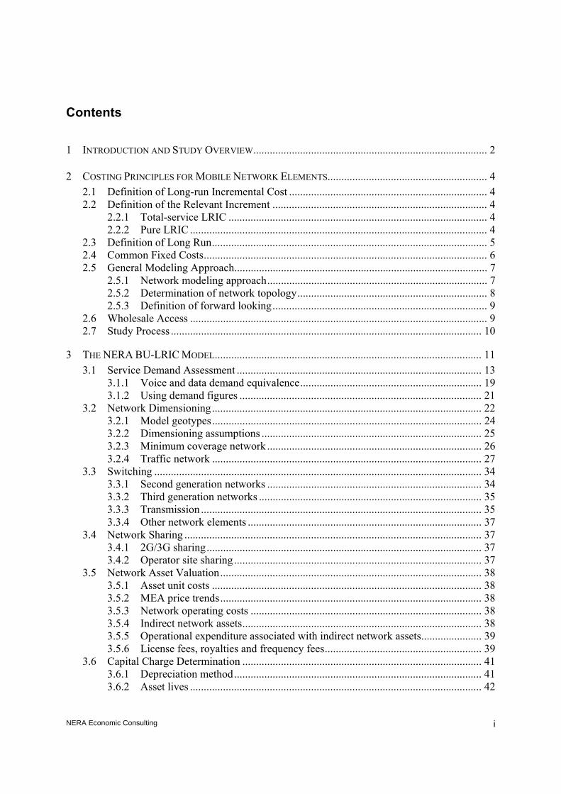
Contents
1 INTRODUCTION AND STUDY OVERVIEW..................................................................................... 2
2 COSTING PRINCIPLES FOR MOBILE NETWORK ELEMENTS.......................................................... 4 2.1 Definition of Long-run Incremental Cost ........................................................................ 4 2.2 Definition of the Relevant Increment .............................................................................. 4
2.2.1 Total-service LRIC .............................................................................................. 4 2.2.2 Pure LRIC ............................................................................................................ 4
2.3 Definition of Long Run.................................................................................................... 5 2.4 Common Fixed Costs....................................................................................................... 6 2.5 General Modeling Approach............................................................................................ 7
2.5.1 Network modeling approach................................................................................ 7 2.5.2 Determination of network topology..................................................................... 8 2.5.3 Definition of forward looking.............................................................................. 9
2.6 Wholesale Access ............................................................................................................ 9 2.7 Study Process ................................................................................................................. 10
3 THE NERA BU-LRIC MODEL................................................................................................. 11 3.1 Service Demand Assessment ......................................................................................... 13
3.1.1 Voice and data demand equivalence.................................................................. 19 3.1.2 Using demand figures ........................................................................................ 21
3.2 Network Dimensioning.................................................................................................. 22 3.2.1 Model geotypes.................................................................................................. 24 3.2.2 Dimensioning assumptions ................................................................................ 25 3.2.3 Minimum coverage network .............................................................................. 26 3.2.4 Traffic network .................................................................................................. 27
3.3 Switching ....................................................................................................................... 34 3.3.1 Second generation networks .............................................................................. 34 3.3.2 Third generation networks ................................................................................. 35 3.3.3 Transmission ...................................................................................................... 35 3.3.4 Other network elements ..................................................................................... 37
3.4 Network Sharing ............................................................................................................ 37 3.4.1 2G/3G sharing.................................................................................................... 37 3.4.2 Operator site sharing .......................................................................................... 37
3.5 Network Asset Valuation............................................................................................... 38 3.5.1 Asset unit costs .................................................................................................. 38 3.5.2 MEA price trends............................................................................................... 38 3.5.3 Network operating costs .................................................................................... 38 3.5.4 Indirect network assets....................................................................................... 38 3.5.5 Operational expenditure associated with indirect network assets...................... 39 3.5.6 License fees, royalties and frequency fees......................................................... 39
3.6 Capital Charge Determination ....................................................................................... 41 3.6.1 Depreciation method.......................................................................................... 41 3.6.2 Asset lives .......................................................................................................... 42

NERA Economic Consulting ii
3.6.3 Cost of capital .................................................................................................... 43 3.7 Calculation of Total LRIC ............................................................................................. 43 3.8 Unit LRIC Costs ............................................................................................................ 44
4 THE MODEL RESULTS .............................................................................................................. 45 4.1 Voice Termination ......................................................................................................... 45 4.2 SMS Termination........................................................................................................... 47 4.3 MMS Termination ......................................................................................................... 49 4.4 Data Termination ........................................................................................................... 51
5 POLICY RECOMMENDATION..................................................................................................... 53
APPENDIX A: MODEL SENSITIVITY ANALYSES ...........................................................................A 55
APPENDIX B: DEMAND FORECAST METHODOLOGIES ................................................................. B 57
APPENDIX C: COST OF CAPITAL CALCULATIONS ........................................................................ C 60

NERA Economic Consulting iii
Figures
FIGURE 1.1 NERA BU-LRIC MODEL SERVICES INCLUDED ............................................................ 2
FIGURE 3.1 OVERVIEW OF NERA’S BU-LRIC MODEL ................................................................. 12
FIGURE 3.2 MARKET SHARES OF OPERATORS IN ISRAEL 1999–2014(E)........................................ 14
FIGURE 3.3 PREDICTED SHARE OF 3G IN ISRAEL 2009–2014......................................................... 16
FIGURE 3.4 SMS TRAFFIC CONVERSION PROCESS ......................................................................... 18
FIGURE 3.5 MMS TRAFFIC CONVERSION PROCESS........................................................................ 19
FIGURE 3.6 WDCMA BUSY HOUR DATA CAPACITY..................................................................... 20
FIGURE 3.7 WDCMA BUSY HOUR VOICE AND DATA EQUIVALENCE............................................ 21
FIGURE 3.8 ILLUSTRATIVE SIMPLIFIED NETWORK TOPOLOGY GSM.............................................. 23
FIGURE 3.9 TRAFFIC DIMENSIONING CALCULATION...................................................................... 29
FIGURE 3.10 EXAMPLE OF GSM FREQUENCY REUSE PATTERN ..................................................... 31
FIGURE 3.11 2G TRANSMISSION AND SWITCHING NETWORK TOPOLOGY ...................................... 34
FIGURE 3.12 3G TRANSMISSION AND SWITCHING NETWORK TOPOLOGY ...................................... 35
FIGURE 3.13 ROUTING FACTOR USE NERA BU-LRIC MODEL..................................................... 44
FIGURE 4.1 NERA BU-LRIC MODEL RESULTS PER MINUTE VOICE TERMINATION 2G................ 45
FIGURE 4.2 NERA BU-LRIC MODEL RESULTS PER MINUTE VOICE TERMINATION 3G................ 46
FIGURE 4.3 NERA BU-LRIC MODEL RESULTS PER SMS TERMINATION 2G................................ 47
FIGURE 4.4 NERA BU-LRIC MODEL RESULTS PER SMS TERMINATION 3G................................ 48
FIGURE 4.5 NERA BU-LRIC MODEL RESULTS PER MMS TERMINATION 2G .............................. 49
FIGURE 4.6 NERA BU-LRIC MODEL RESULTS PER MMS TERMINATION 3G .............................. 50
FIGURE 4.7 NERA BU-LRIC MODEL RESULTS PER MB DATA TERMINATION 2G ....................... 51

NERA Economic Consulting iv
FIGURE 4.8 NERA BU-LRIC MODEL RESULTS PER MB DATA TERMINATION 3G ....................... 52
NERA Economic Consulting v
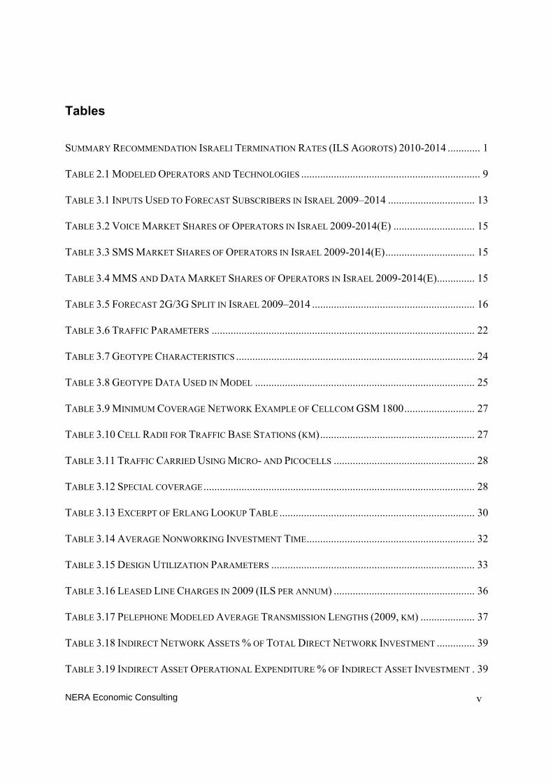
Tables
SUMMARY RECOMMENDATION ISRAELI TERMINATION RATES (ILS AGOROTS) 2010-2014 ............ 1
TABLE 2.1 MODELED OPERATORS AND TECHNOLOGIES .................................................................. 9
TABLE 3.1 INPUTS USED TO FORECAST SUBSCRIBERS IN ISRAEL 2009–2014 ................................ 13
TABLE 3.2 VOICE MARKET SHARES OF OPERATORS IN ISRAEL 2009-2014(E) .............................. 15
TABLE 3.3 SMS MARKET SHARES OF OPERATORS IN ISRAEL 2009-2014(E)................................. 15
TABLE 3.4 MMS AND DATA MARKET SHARES OF OPERATORS IN ISRAEL 2009-2014(E).............. 15
TABLE 3.5 FORECAST 2G/3G SPLIT IN ISRAEL 2009–2014 ............................................................ 16
TABLE 3.6 TRAFFIC PARAMETERS ................................................................................................. 22
TABLE 3.7 GEOTYPE CHARACTERISTICS ........................................................................................ 24
TABLE 3.8 GEOTYPE DATA USED IN MODEL ................................................................................. 25
TABLE 3.9 MINIMUM COVERAGE NETWORK EXAMPLE OF CELLCOM GSM 1800.......................... 27
TABLE 3.10 CELL RADII FOR TRAFFIC BASE STATIONS (KM)......................................................... 27
TABLE 3.11 TRAFFIC CARRIED USING MICRO- AND PICOCELLS .................................................... 28
TABLE 3.12 SPECIAL COVERAGE.................................................................................................... 28
TABLE 3.13 EXCERPT OF ERLANG LOOKUP TABLE ........................................................................ 30
TABLE 3.14 AVERAGE NONWORKING INVESTMENT TIME.............................................................. 32
TABLE 3.15 DESIGN UTILIZATION PARAMETERS ........................................................................... 33
TABLE 3.16 LEASED LINE CHARGES IN 2009 (ILS PER ANNUM) .................................................... 36
TABLE 3.17 PELEPHONE MODELED AVERAGE TRANSMISSION LENGTHS (2009, KM) .................... 37
TABLE 3.18 INDIRECT NETWORK ASSETS % OF TOTAL DIRECT NETWORK INVESTMENT .............. 39
TABLE 3.19 INDIRECT ASSET OPERATIONAL EXPENDITURE % OF INDIRECT ASSET INVESTMENT . 39

NERA Economic Consulting vi
TABLE 3.20 3G LICENSE FEES ....................................................................................................... 40
TABLE 3.21 ROYALTY RATES (%) ................................................................................................. 40
TABLE 3.22 SPECTRUM FREQUENCY FEES (ILS)............................................................................ 41
TABLE 3.23 ASSET LIVES............................................................................................................... 43
TABLE 3.24 PRETAX NOMINAL COST OF CAPITAL ISRAELI MNO 2009 ......................................... 43
TABLE 4.1 NERA BU-LRIC MODEL RESULTS PER-MINUTE VOICE TERMINATION 2009–2014 ... 46
TABLE 4.2 NERA BU-LRIC MODEL RESULTS PER SMS TERMINATION 2009–2014.................... 48
TABLE 4.3 NERA BU-LRIC MODEL RESULTS PER MMS TERMINATION 2009–2014 .................. 50
TABLE 4.4 NERA BU-LRIC MODEL RESULTS PER MB DATA TERMINATION 2009–2014 ........... 52
TABLE 5.1 VOICE (PER MINUTE) POLICY RECOMMENDATION ........................................................ 53
TABLE 5.2 SMS (PER MESSAGE) POLICY RECOMMENDATION........................................................ 54
TABLE 5.3 POLICY RECOMMENDATION SUMMARY........................................................................ 54

.הסגנון אינו מוגדר! שגיאה
NERA Economic Consulting 1
Executive Summary
NERA Economic Consulting (NERA) was commissioned by the Israel Ministry of Communications (MOC) and Ministry of Finance (MOF) to construct a bottom-up cost model to examine the charges for network elements in the mobile telephony market in Israel and, if appropriate, recommend changes to the regulated current interconnection rates.
In line with international best practices and a previous cost model constructed for the MOC and the MOF, we constructed a bottom-up LRIC model. In deriving the input values for this model, we solicited specific data from the Israeli operators, ranging from current demand information to modern equivalent asset prices, operating expenses, and price trends. We also requested market level data from the MOC, such as spectrum costs or the type and number of base transceiver stations (BTSs). Although we received some data from the operators, for many other necessary inputs to the cost model, we had to rely on international benchmark data, forecasts, or commercially and publicly available data sources. We made a conscious effort to use all the data received from the Israeli operators unless we found the data to be inconsistent with international benchmarks.
The modeling approach is documented in this report. Furthermore, we prepared a technical report that further explains the working of the NERA BU-LRIC model. The model itself is programmed in Microsoft Excel and has been submitted to the MOC and the MOF. It is accompanied with company-specific input sheets for Cellcom, Partner and Pelephone.
As we detail in this report, the principal finding of our study is that current voice and SMS termination rates are significantly above current cost levels. In the summary table below, we present the voice and SMS termination costs from 2009–2014. We recommend that the MOC set voice and SMS at average blended cost, as shown in the table below.1 Specifically, we recommend that all termination rates be symmetric in that the same rate would apply for all networks regardless of whether the network is 2G or 3G or if it terminates on Cellcom’s, Partner’s, or Pelephone’s networks.
Summary Recommendation Israeli Termination Rates (ILS Agorots)
2010-2014
2010 2011 2012 2013 2014
Voice (per minute) 4.14 3.54 3.11 2.80 2.57
SMS (per message) 0.19 0.17 0.16 0.14 0.13
1 Average blended rates represent the weighted average 2G and 3G costs for each operator, using relative
traffic proportions as weights. We then average these blended rates across all three operators to arrive at our recommended termination rates.
.הסגנון אינו מוגדר! שגיאה
NERA Economic Consulting 2
1 Introduction and Study Overview
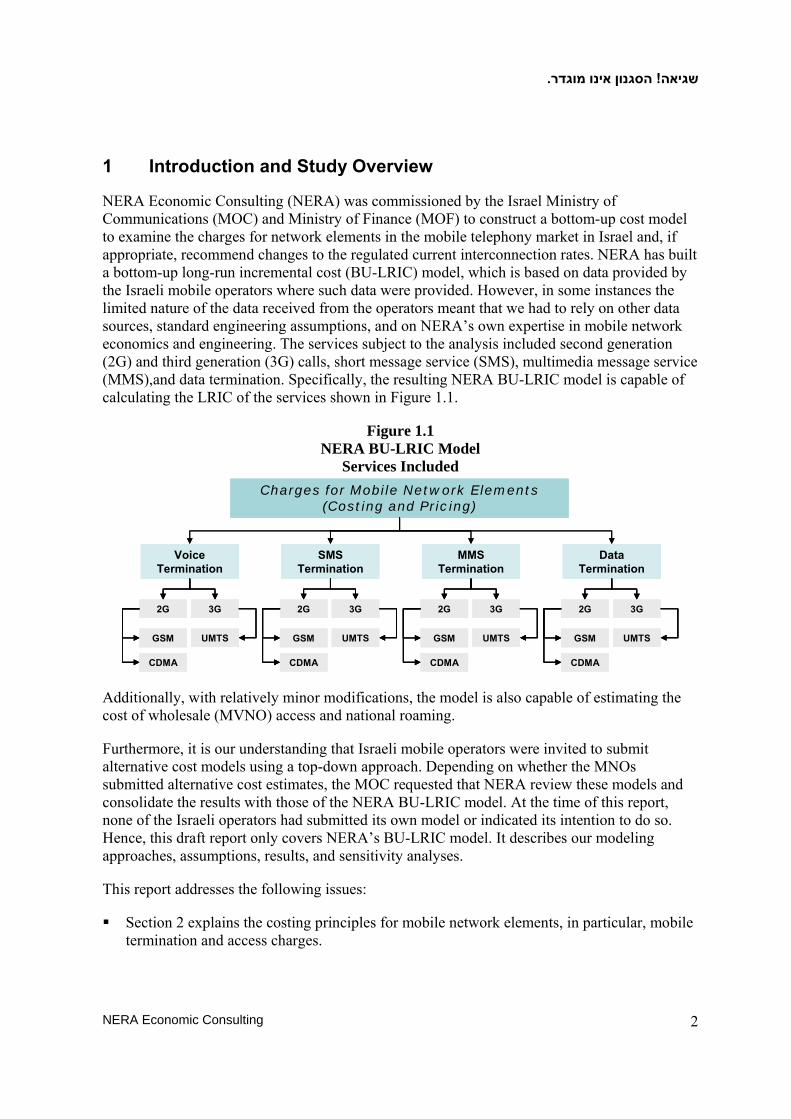
NERA Economic Consulting (NERA) was commissioned by the Israel Ministry of Communications (MOC) and Ministry of Finance (MOF) to construct a bottom-up cost model to examine the charges for network elements in the mobile telephony market in Israel and, if appropriate, recommend changes to the regulated current interconnection rates. NERA has built a bottom-up long-run incremental cost (BU-LRIC) model, which is based on data provided by the Israeli mobile operators where such data were provided. However, in some instances the limited nature of the data received from the operators meant that we had to rely on other data sources, standard engineering assumptions, and on NERA’s own expertise in mobile network economics and engineering. The services subject to the analysis included second generation (2G) and third generation (3G) calls, short message service (SMS), multimedia message service (MMS),and data termination. Specifically, the resulting NERA BU-LRIC model is capable of calculating the LRIC of the services shown in Figure 1.1.
Figure 1.1 NERA BU-LRIC Model
Services Included Charges for Mobile Network Elements
(Costing and Pricing)
2G
CDMA
3G
GSM UMTS
VoiceTermination
SMSTermination
2G
CDMA
3G
GSM UMTS
MMSTermination
2G
CDMA
3G
GSM UMTS
DataTermination
2G
CDMA
3G
GSM UMTS
Charges for Mobile Network Elements(Costing and Pricing)
2G
CDMA
3G
GSM UMTS
VoiceTermination
2G
CDMA
3G
GSM UMTS
VoiceTermination
SMSTermination
2G
CDMA
3G
GSM UMTS
SMSTermination
2G
CDMA
3G
GSM UMTS
MMSTermination
2G
CDMA
3G
GSM UMTS
MMSTermination
2G
CDMA
3G
GSM UMTS
DataTermination
2G
CDMA
3G
GSM UMTS
DataTermination
2G
CDMA
3G
GSM UMTS
Additionally, with relatively minor modifications, the model is also capable of estimating the cost of wholesale (MVNO) access and national roaming.
Furthermore, it is our understanding that Israeli mobile operators were invited to submit alternative cost models using a top-down approach. Depending on whether the MNOs submitted alternative cost estimates, the MOC requested that NERA review these models and consolidate the results with those of the NERA BU-LRIC model. At the time of this report, none of the Israeli operators had submitted its own model or indicated its intention to do so. Hence, this draft report only covers NERA’s BU-LRIC model. It describes our modeling approaches, assumptions, results, and sensitivity analyses.
This report addresses the following issues:
Section 2 explains the costing principles for mobile network elements, in particular, mobile termination and access charges.

.הסגנון אינו מוגדר! שגיאה
NERA Economic Consulting 3
Section 3 provides details of the NERA BU-LRIC model, including its methodology, input data, algorithms and equations, and scenario and sensitivity analyses.
In section 4, we present the company-specific model results.
Section 5 offers our policy recommendations, including LRIC estimates, the markup over LRIC to recover common fixed costs, and finally the mobile termination rate recommendations.
This report is accompanied by a detailed technical report and user manual.
.הסגנון אינו מוגדר! שגיאה
NERA Economic Consulting 4
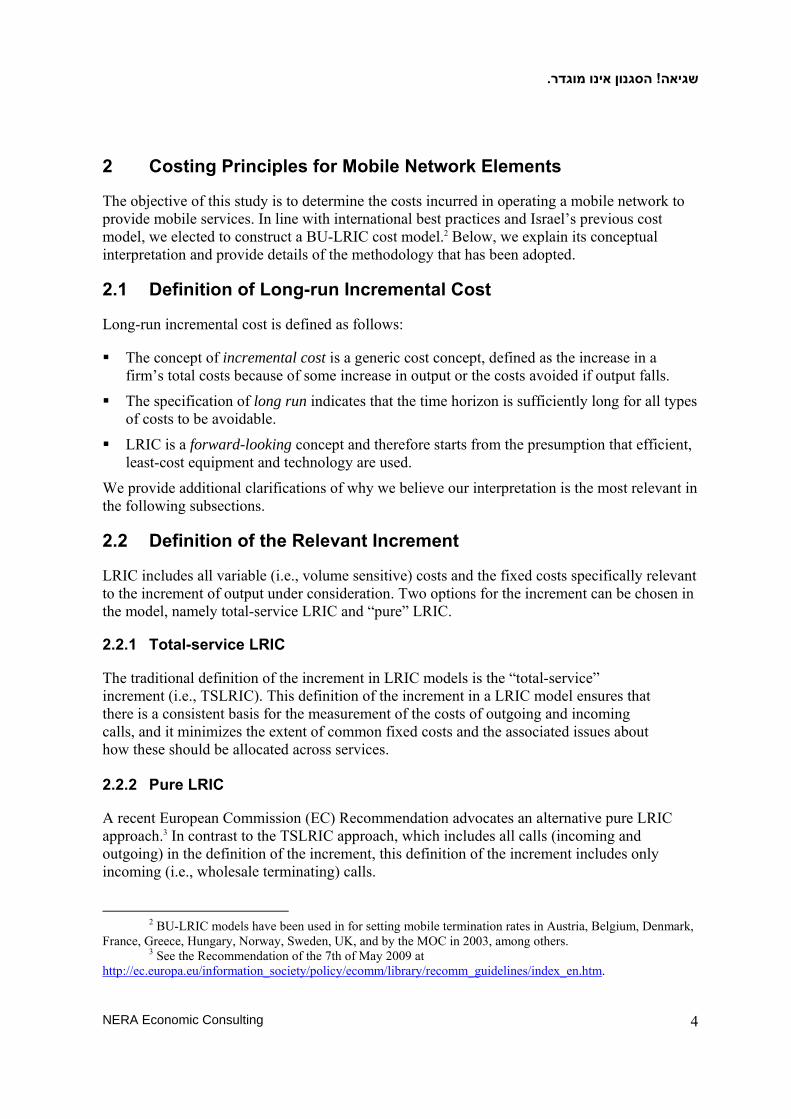
2 Costing Principles for Mobile Network Elements
The objective of this study is to determine the costs incurred in operating a mobile network to provide mobile services. In line with international best practices and Israel’s previous cost model, we elected to construct a BU-LRIC cost model.2 Below, we explain its conceptual interpretation and provide details of the methodology that has been adopted.
2.1 Definition of Long-run Incremental Cost
Long-run incremental cost is defined as follows:
The concept of incremental cost is a generic cost concept, defined as the increase in a firm’s total costs because of some increase in output or the costs avoided if output falls.
The specification of long run indicates that the time horizon is sufficiently long for all types of costs to be avoidable.
LRIC is a forward-looking concept and therefore starts from the presumption that efficient, least-cost equipment and technology are used.
We provide additional clarifications of why we believe our interpretation is the most relevant in the following subsections.
2.2 Definition of the Relevant Increment
LRIC includes all variable (i.e., volume sensitive) costs and the fixed costs specifically relevant to the increment of output under consideration. Two options for the increment can be chosen in the model, namely total-service LRIC and “pure” LRIC.
2.2.1 Total-service LRIC
The traditional definition of the increment in LRIC models is the “total-service” increment (i.e., TSLRIC). This definition of the increment in a LRIC model ensures that there is a consistent basis for the measurement of the costs of outgoing and incoming calls, and it minimizes the extent of common fixed costs and the associated issues about how these should be allocated across services.
2.2.2 Pure LRIC
A recent European Commission (EC) Recommendation advocates an alternative pure LRIC approach.3 In contrast to the TSLRIC approach, which includes all calls (incoming and outgoing) in the definition of the increment, this definition of the increment includes only incoming (i.e., wholesale terminating) calls.
2 BU-LRIC models have been used in for setting mobile termination rates in Austria, Belgium, Denmark,
France, Greece, Hungary, Norway, Sweden, UK, and by the MOC in 2003, among others. 3 See the Recommendation of the 7th of May 2009 at
http://ec.europa.eu/information_society/policy/ecomm/library/recomm_guidelines/index_en.htm.

.הסגנון אינו מוגדר! שגיאה
NERA Economic Consulting 5
The choice of increment (i.e., TSLRIC or pure LRIC) has a direct impact on the allocation of common fixed costs. Specifically, if the TSLRIC approach is selected, the resulting costs include all costs that are fixed and common to incoming and outgoing calls. As a result, the average incremental cost of call termination will lie above the marginal cost of call termination, and the remaining joint and common fixed costs will be relatively small. In this instance, the common fixed costs include the costs of the minimum coverage network, radio spectrum, and network management systems.
In contrast, if the EC’s pure LRIC approach is selected, then only the fixed costs that are specific to terminating calls (which are relatively small) are included in the incremental cost of call termination. This means that the incremental cost will approach marginal cost and hence will be lower than in the first scenario.
The implications of the pure LRIC approach for the recovery of fixed and common costs have sparked a vigorous debate.4 For example, respondents (including national regulatory authorities) have questioned the justification provided for the proposed change to a pure LRIC approach. In particular, although the EC argues for pure LRIC because it would “facilitate efficient cost recovery,” it is not clear from its proposals where common fixed costs would be recovered.
Moreover, if all service prices were set on a pure LRIC basis, common costs would not be recovered, and the company concerned would operate at a loss. Hence, if companies were forced to operate at a loss on mobile termination, they would attempt to increase prices for retail services. This, so-called waterbed effect, stands to defeat the EU’s aim of efficient cost recovery and enhanced consumer welfare. Based on these considerations, and the fact that, to our knowledge, no national regulatory authority has yet implemented MTRs based on a pure LRIC approach, we recommend that the increment include all (incoming and outgoing) calls consistent with the TSLRIC approach. Notwithstanding this, the NERA BU-LRIC model has a user-adjustable option to calculate LRICs based on either the TSLRIC or the pure LRIC approach. We discuss the sensitivity of the LRIC estimates to the choice of increment in Appendix A to this report.
2.3 Definition of Long Run
The specification of long run requires that the time horizon is sufficiently long for all types of costs to be avoidable. Alternatively, long run has been defined as:
… the time horizon within which the operator can undertake capital investment or divestment to increase or decrease the capacity of its existing productive assets. Thus a very long time horizon is observed in which all costs, including investment capital and all costs related to network capacity, are potentially variable with no fixed element.5
4 See the responses to the European Commission’s consultation process, available from
http://ec.europa.eu/information_society/policy/ecomm/library/public_consult/termination_rates/index_en.htm. 5 European Union Independent Regulators Group, “Principles of implementation and best practice
regarding FL-LRIC cost modeling,” as decided by the Independent Regulators Group, November 24, 2000, p. 6.
.הסגנון אינו מוגדר! שגיאה
NERA Economic Consulting 6
The definition of long run, which is embedded in the NERA BU-LRIC model, assumes that all costs are avoidable.
2.4 Common Fixed Costs
Common fixed costs are those costs that are not incremental to any one product or service. Consequently, they are not included in LRIC. However, as discussed above, mobile operators must recover common fixed costs to remain viable. Hence, consistent with international best practices, we recommend that LRIC be marked up to enable efficiently incurred common fixed costs to be recovered. Notwithstanding this, the NERA BU-LRIC model allows users also to run LRIC estimates without a markup for common costs.
Two main methods exist by which common fixed costs can be recovered—equi-proportional mark-up (EPMU) and Ramsey pricing. Under EPMU, common fixed costs are recovered in proportion to the incremental costs of the services. Ramsey pricing, on the other hand, recovers common fixed costs in inverse proportion to the price elasticities of demand of different services.
The U.S. Federal Communications Commission (FCC) has recognized the need to take into account those costs shared by groups of network elements and those common to all services and elements (e.g., corporate overheads). It noted that:
Because forward-looking common costs are consistent with our forward-looking, economic cost paradigm, a reasonable measure of such costs shall be included in the prices for interconnection and access to network elements.6
The FCC accepted EPMU as an appropriate basis for recovering common fixed costs but explicitly ruled out Ramsey pricing because of concerns that it might “unreasonably limit the extent of entry into local exchange markets by allocating more costs to, and thus raising the prices of, the most critical bottleneck inputs, the demand for which tends to be relatively inelastic.”7
The Independent Regulators Group (IRG), although recognizing that it was standard practice to mark up incremental costs so as to recover a reasonable share of common fixed costs, did not commit itself to, or rule out, any of the possible allocation methods. More specifically, it noted the following:
There are various methods of recovering common costs across a range of services. From an economic point of view distortion is minimized by recovery of common costs according to Ramsey Pricing. This recovers common costs from the products based on the products’ relative marginal cost of production and price elasticities. However, this method of recovering common costs requires robust and detailed information on elasticities, which is often hard to find. The alternative is to recover common costs according to an accounting rule. For example, if the common input were used to produce two separate,
6 Federal Communications Commission, FCC 96-325, August 1996, ¶ 694. 7 Ibid., ¶ 696.

.הסגנון אינו מוגדר! שגיאה
NERA Economic Consulting 7
regulated services, one simple rule would be to split the common cost equally between the two services. Another example would be to recover common costs in proportion to the incremental cost of the two services. This method of allocating costs is known as equal proportionate mark-up (EPMU).8
Given the complexity of Ramsey pricing and the difficulty of obtaining price elasticities, this method has not found widespread use. Based on these considerations, the NERA BU-LRIC model employs EPMU.
We note that estimated wholesale costs exclude retail costs as these are not relevant to providing call conveyance for interconnection. Retail costs include sales, advertising, marketing, subscriber acquisition costs, and the costs of retail subscriber billing and customer care. In some jurisdictions, a further markup is added to allow for the recovery, at least for a specified period of time, of stranded and legacy costs.
2.5 General Modeling Approach
The approach we have adopted in this analysis is commonly described as a bottom-up model. Bottom-up modeling involves the construction of an engineering model to estimate the cost of building a mobile operator’s network, assuming that all costs are avoidable (in the long run) and that the network is built using forward-looking technologies. This general approach requires that additional, more specific modeling decisions have to be made. We discuss each of these below.
2.5.1 Network modeling approach
In common with other telecommunications cost modeling studies, we use network components as the building blocks of the cost model. Specifically, the NERA BU-LRIC model derives the costs of the services based on the different components of the network, such as mobile switching centers (MSC), base transceiver stations (BTS), and base station controllers(BSC). This approach is adopted for two principal reasons. First, a component-based approach is the most practical approach as component costs can be identified more readily in a bottom-up model than other building increments (such as services or network layers). Second, and more importantly, the costs imposed on the network by different forms of usage (e.g., mobile call termination) are directly related to the components utilized by each of the services. If, for example, an operator provides 2G mobile call termination interconnection to a competitor, it must provide capacity in the tandem switch, the home location register (HLR), the MSC, the BSC, the BTS and the associated communications linkages. However, the competitor imposes no costs on the terminating operator’s general packet radio service (GPRS) data network elements.
To derive service costs based on component costs, the NERA BU-LRIC model uses so-called routing factors. Routing factors specify the average number of units of each network component used by a particular type of service. Routing factors are commonly measured by the
8 European Union Independent Regulators Group, Principles of Implementation and Best Practice Regarding
FL-LRIC Cost Modelling, November 24, 2000, p. 5
.הסגנון אינו מוגדר! שגיאה
NERA Economic Consulting 8
operators from traffic samples and are often already used as a means of establishing the cost of retail call services. In the case of interconnection services, some of the routing factors can be established almost by definition. For example, mobile call termination will make use of a one BTS, while an on-net call will make use of two BTSs.
In order to model the different technologies, as shown in Figure 1.1 above, the model uses a “wide routing factor matrix,” which includes routing factors for all the modeled technologies. The values in this matrix are based on the operators’ submissions, but where necessary (e.g., if factors were not provided or were anomalous) they have been amended and supplemented by NERA based on telecommunications engineering knowledge and principles.
2.5.2 Determination of network topology
Another issue to be considered is whether the modeled network topology mirrors the networks currently in place or whether the model assumes that forward-looking LRIC costs are based on a fully efficient operator that builds an ideal topology to match future demand levels. These two topology concepts are commonly referred to as “scorched node” and “scorched earth.” Specifically, scorched node is an approach that takes the current location and number of network nodes as the basis for the modeled network topology. Specific to the present project, modeling based on a scorched node topology would mean that the location and number of BTSs, Node Bs, BSCs, radio network controllers (RNCs), MSCs, and other equipment are given. Alternatively, scorched earth is an approach where the location and number of network nodes are determined based on an optimal network design, taking into account current and future demand levels.
Consistent with the MOC’s prior cost modeling efforts, we determined that the model should have the number of nodes that best reflects the actual networks in Israel. This “modified” scorched node approach reflects international best practices and implies that “the technology at and in between existing switching nodes is optimized to meet the demands of a forward-looking efficient operator.”9 Furthermore, such an approach takes into account:
The efficient choices of a hypothetical new entrant, which are constrained by the current and future availability and commercial conditions associated with site procurement. Therefore, it relies upon statistics about the design of the actual operators’ networks as predictors of the network design constraints faced.
Network design is complicated as it involves a very large number of factors and design parameters, not all of which are known, and this can make optimal network design uncertain.
Networks develop over time in response to changes in forecasted demand in addition to technological evolution and uncertainty—not the theoretical limits of efficiency.
9 European Union Independent Regulators Group, “Principles of implementation and best practice
regarding FL-LRIC cost modeling,” as decided by the Independent Regulators Group, November 24, 2000, p. 3.
.הסגנון אינו מוגדר! שגיאה
NERA Economic Consulting 9
2.5.3 Definition of forward looking
The forward-looking, efficient market outcome philosophy, which informs the LRIC approach, requires that the asset values in the model be valued using the costs of an efficient entrant, rather than the historic costs incurred by the incumbent mobile network operators (MNOs). In practice, this means that assets are valued based on the costs of replacing them with modern equivalent assets (MEAs). An MEA is the lowest-cost asset that serves the same function as the asset being valued. It incorporates the latest available technology and is the asset that a new entrant might be expected to employ.10 However, the model retains the flexibility to vary network capacities and traffic volumes for a set of different scenarios based on the input data from Cellcom, Partner, and Pelephone.
In compliance with the MOC’s stated goal of forecasting for a period of approximately five years starting in 2009, the NERA model forecasts MEA prices and technological development from 2009–2014, based on GSM, CDMA, and WCDMA technologies.11 Specifically, as shown in Table 2.1 below, the model produces network charges for the following operators and technologies.
Table 2.1 Modeled Operators and Technologies
Operator 2G Network 3G Network
Cellcom GSM 1800 WCDMA Release 7 dual band
Partner GSM dual band 900/1800 WCDMA Release 7 2100
Pelephone CDMA 850 WCDMA Release 7 dual band Source: NERA
As Table 2.1 shows, each existing operator uses a different 2G technology and is modeled to reflect this. Furthermore, based on the Israeli operators’ submissions and consistent with a forward-looking modeling approach, NERA has modeled all three operators as having WCDMA Release 7 3G networks. Specifically, in the case of Partner, this uses its 2100 frequency allocation. For Cellcom and Pelephone dual band assumptions are used.
2.6 Wholesale Access
The model produces network element costs which are aggregated to derive service costs. Although the model has been designed with mobile termination in mind, with relatively minor modifications this process can be extended to obtain the cost of wholesale access. Wholesale access can take the form of either MVNO access or MNO access (i.e., national roaming).
10 European Union Independent Regulators Group, “Principles of Implementation and Best Practice
Regarding FL-LRIC Cost Modelling,” 24 November 2000, p. 6 11 See “State of Israel, Ministry of Communications, Project Description: Consulting Services Regarding
Charges for Mobile Network Elements, May 2009,” and the MOC’s responses to clarification questions received from bidding consulting firms.
.הסגנון אינו מוגדר! שגיאה
NERA Economic Consulting 10
2.7 Study Process
In order to collect the necessary data for the NERA BU-LRIC model, NERA prepared a comprehensive data request form in Microsoft Excel, along with a document describing the necessary data for the model. This data request was submitted to Cellcom, Partner, Pelephone, and MIRS. Furthermore, following the submission of the data request, NERA had meetings with all incumbent mobile operators in Jerusalem to clarify any questions they might have. We also provided contact information to which questions regarding the data forms could be sent.
Partial data was submitted by the operators in several stages. NERA combined all data received and examined the data for accuracy and consistency. We also had several rounds of clarifications with some of the operators to ensure the proper understanding and use of the data. The resulting data was then used as source data for the NERA BU-LRIC model.
However, despite NERA’s comprehensive data request and efforts, considerable data were not provided by the operators. Hence, where data were not provided by the operators, or if NERA considered the data received to be inconsistent with other data, we used data from the MOC. Where no data were available from the MOC, we drew upon our previous experience of mobile costing work and employed commercially and publicly available data from other jurisdictions.

.הסגנון אינו מוגדר! שגיאה
NERA Economic Consulting 11
3 The NERA BU-LRIC Model
Most generally, the NERA BU-LRIC model involves the following tasks for each relevant technology.
1. Service demand assessment (What demand will the network serve?): This is the starting point of the NERA BU-LRIC model. It forecasts the number of subscribers and the traffic volume for each type of service during the study period (2009–2014). Company-specific demand levels are then calculated based on current and forecasted market shares.
2. Network dimensioning (What network components, size, and quantity are required?): Based on the forecast demand, the model calculates the current and future capacity of the network for each technology based on the coverage requirement, traffic distribution, quality of service, and so on. Next, the model calculates the physical quantities of components required given the capacity of each network element (e.g., the number of subscribers a home location register can serve).
3. Network asset valuation (What is the current and future cost of the network components?): Having established the required quantities of network equipment, the associated capital expenditures are calculated by applying MEA unit cost and price trends. The model also adds an allowance for indirect network assets such as buildings, vehicles, computers, and office equipment.
4. Capital charge determination (What is the annual capital charge for the network investment?): Network capital expenditures are incurred to provide mobile services. To derive the annual costs of network components and hence services, it is necessary to annualize the cost of network assets, using an appropriate depreciation method and the required return on capital.
5. Calculation of total costs (What is the total cost of operating each network element?): The model calculates operating expenditures for each type of equipment to capture the cost of network maintenance and operation and support. It then marks up the operating expenditures to allow for indirect network operating costs. The total (direct and indirect) operational expenditures are added to the capital charge to arrive at the total LRIC cost.
6. Unit LRIC costs (What are the long-run average incremental costs allocated to specific services and network elements?): In this final step, the model computes the unit LRIC cost of each service. This involves the use of routing factors. For example, the average requirements of an incoming call can be defined in terms of the number of base stations the call passes through, the number and length of the transmission links, the number of switching stages, and so on. These routing factors are then multiplied by the volume of each service. The volume-weighted routing factors, in turn, are used to allocate the cost of each of these network elements, including both capital and operating costs, in order to derive the total network cost per minute for an incoming call.
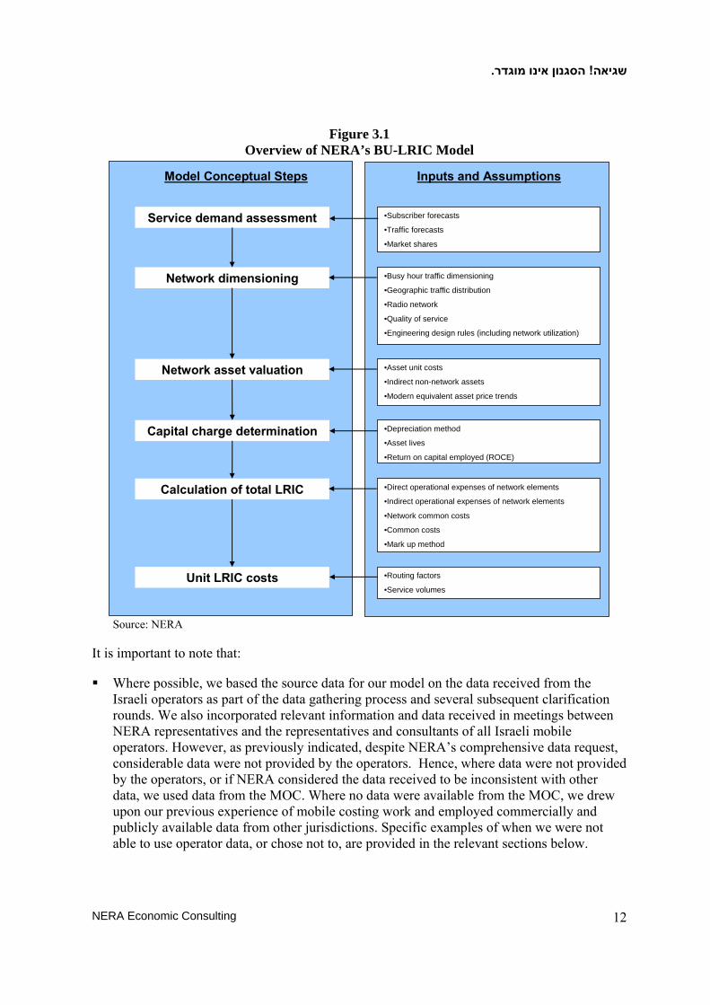
The general NERA mobile costing approach is summarized in Figure 3.1.
.הסגנון אינו מוגדר! שגיאה
NERA Economic Consulting 12
Figure 3.1 Overview of NERA’s BU-LRIC Model
Service demand assessment
Network dimensioning
Network asset valuation
Unit LRIC costs
Calculation of total LRIC
•Subscriber forecasts
•Traffic forecasts
•Market shares
•Busy hour traffic dimensioning
•Geographic traffic distribution
•Radio network
•Quality of service
•Engineering design rules (including network utilization)
•Asset unit costs
•Indirect non-network assets
•Modern equivalent asset price trends
•Direct operational expenses of network elements
•Indirect operational expenses of network elements
•Network common costs
•Common costs
•Mark up method
•Routing factors
•Service volumes
Capital charge determination •Depreciation method
•Asset lives
•Return on capital employed (ROCE)
Model Conceptual Steps Inputs and Assumptions
Source: NERA
It is important to note that:
Where possible, we based the source data for our model on the data received from the Israeli operators as part of the data gathering process and several subsequent clarification rounds. We also incorporated relevant information and data received in meetings between NERA representatives and the representatives and consultants of all Israeli mobile operators. However, as previously indicated, despite NERA’s comprehensive data request, considerable data were not provided by the operators. Hence, where data were not provided by the operators, or if NERA considered the data received to be inconsistent with other data, we used data from the MOC. Where no data were available from the MOC, we drew upon our previous experience of mobile costing work and employed commercially and publicly available data from other jurisdictions. Specific examples of when we were not able to use operator data, or chose not to, are provided in the relevant sections below.

.הסגנון אינו מוגדר! שגיאה
NERA Economic Consulting 13
The costs of an individual service cannot be modeled in isolation of other services. This is because a large number of network components are used by more than one service (for example a BTS is used to carry voice, SMS, and GPRS data services). Therefore, we have included a comprehensive set of services in the model.
The model provides a simulation of the mobile networks in Israel, but there is a limit to the number of network elements that can be reasonably modeled. Thus, we have deliberately limited the model to the most relevant and distinguishable network components rather than attempt to model every single component of a mobile network.
Where possible, we compared the quantities of network elements contained in the model with those actually in the operators’ networks.
3.1 Service Demand Assessment
The first stage in deriving LRIC costs is to estimate the amount of capacity required to handle the subscribers and market traffic volumes (i.e., the demand) in Israel during the study period. Specifically, as shown in the “1 Inputs” sheet of the NERA BU-LRIC model, we forecast the following for the period 2009–2014:
Total mobile subscribers in Israel
Operator specific mobile subscribers
Operator market shares
Annual traffic splits
Market traffic volumes
In forecasting the demand levels, NERA relied on data received from the operators, the MOC, and publicly and commercially available databases. The specific methodologies used to forecast each variable are described in Appendix B to this report.
The service demand assessment commences with forecasting the total number of mobile subscribers from 2009–2014, based on the population and mobile penetration rates in Israel. This is summarized in Table 3.1 below.
Table 3.1 Inputs Used to Forecast Subscribers in Israel
2009–2014
2009 2010 2011 2012 2013 2014
Population 7,505,503 7,639,351 7,775,586 7,914,251 8,055,388 8,199,043
Penetration 124% 126% 128% 130% 132% 134%
Percent 3G 29.5% 32.8% 36.6% 40.9% 45.9% 51.5% Source: NERA

.הסגנון אינו מוגדר! שגיאה
NERA Economic Consulting 14
Next, based on data received from the operators, we forecasted market shares which allowed us to derive the operators’ respective traffic volumes12. Specifically, we estimated the 2009 market shares based on the operators’ declarations. Market shares for 2010 were forecasted using operator-specific average-growth rates in market share between 2007 and 2009. We assumed that the MIRS market shares remain unchanged during the study period, and by 2016 a new 3G entrant will obtain 10 percent of the residential market segment and 5 percent of the business market segment. We split up market shares into voice, SMS, MMS and data market shares. We understand that these assumptions are in line with general expectations. We further assumed that the market share of the 3G entrant would come at the expense of all the other major operators with each losing an equal percentage of its market share to the entrant each year. The forecasted market shares are illustrated in Figure 3.2 and shown in Tables 3.2 to 3.4 below.
Figure 3.2 Market Shares of Operators in Israel
1999–2014(E)
0%
10%
20%
30%
40%
50%
1999 2000 2001 2002 2003 2004 2005 2006 2007 2008 2009E 2010E 2011E 2012E 2013E 2014E
Mar
ket S
hare
Cellcom Pelephone Partner MIRS 3G Entrant Source: NERA
12 Specifically, we created separate market shares for voice, SMS and also MMS and data. Due to data
limitations, we assumed the MMS and data markets followed Israel-wide market share trends, shown in Figure 3.2.

.הסגנון אינו מוגדר! שגיאה
NERA Economic Consulting 15
Table 3.2 Voice Market Shares of Operators in Israel
2009-2014(E)
2009E 2010E 2011E 2012E 2013E 2014ECellcom 33.3% 33.4% 32.8% 32.2% 31.7% 31.1%Partner 33.4% 33.4% 32.8% 32.3% 31.7% 31.1%Pelephone 28.2% 28.1% 27.6% 27.0% 26.4% 25.8%MIRS 5.1% 5.1% 5.1% 5.1% 5.1% 5.1%3G Entrant 0.0% 0.0% 1.7% 3.5% 5.2% 6.9%
Source: NERA
Table 3.3 SMS Market Shares of Operators in Israel
2009-2014(E)
2009E 2010E 2011E 2012E 2013E 2014ECellcom 31.0% 31.1% 30.5% 29.9% 29.3% 28.8%Partner 42.8% 42.9% 42.3% 41.7% 41.2% 40.6%Pelephone 21.6% 21.5% 20.9% 20.4% 19.8% 19.2%MIRS 4.6% 4.6% 4.6% 4.6% 4.6% 4.6%3G Entrant 0.0% 0.0% 1.7% 3.5% 5.2% 6.9%
Source: NERA
Table 3.4 MMS and Data Market Shares of Operators in Israel
2009-2014(E)
2009E 2010E 2011E 2012E 2013E 2014ECellcom 34.7% 34.8% 34.2% 33.6% 33.1% 32.5%Partner 32.1% 32.2% 31.6% 31.0% 30.4% 29.9%Pelephone 28.1% 28.1% 27.5% 26.9% 26.3% 25.8%MIRS 5.0% 5.0% 5.0%` 5.0% 5.0% 5.0%3G Entrant 0.0% 0.0% 1.7% 3.5% 5.2% 6.9%
Source: NERA
The operator volumes were then further disaggregated into 2G and 3G traffic volumes, using the forecasts in Table 3.5 below. Starting with the traffic splits as declared by the operators, we assumed that the proportion of traffic over each operator’s 2G network would decrease in the same proportion as the percentage of 2G subscribers in the total market. This percentage, in turn, is calculated based on the number of 3G subscribers in the total market.

.הסגנון אינו מוגדר! שגיאה
NERA Economic Consulting 16
Table 3.5 Forecast 2G/3G Split in Israel
2009–2014
2009 2010 2011 2012 2013 2014
2G 75% 71% 67% 63% 58% 52% Cellcom
3G 25% 29% 33% 37% 42% 48%
2G 51% 49% 46% 43% 39% 35% Partner
3G 49% 51% 54% 51% 61% 65%
2G 60% 57% 54% 50% 46% 41% Pelephone
3G 40% 43% 46% 50% 54% 59% Source: NERA analysis based on operator submissions
The forecasted percentage of 3G subscribers is the result of an econometric analysis based on migration patterns and other attributes of 47 countries for which data were available around the world. This model predicts the following evolution of 3G in Israel.
Figure 3.3 Predicted Share of 3G in Israel
2009–2014
0%
10%
20%
30%
40%
50%
60%
70%
80%
2008 2009 2010 2011 2012 2013 2014
Percentage 3GPercentage 2G
Source: NERA analysis
Having forecast the total number of subscribers, the market shares of different operators, and the traffic split between 2G and 3G, we forecasted the market traffic volumes. This involved

.הסגנון אינו מוגדר! שגיאה
NERA Economic Consulting 17
estimating total call minutes and total successful calls for each of the following wireless services:
Mobile to mobile – on-net
Mobile to mobile – off-net
Mobile to fixed
Mobile to international
Fixed to mobile (termination)
Other to mobile (termination)
Mobile to voicemail
Fixed to voicemail
International roaming
We also forecasted the volumes of SMS, MMS, GPRS, and WCDMA traffic. To convert SMS traffic into a voice-minute equivalent, we first determined the average size of an SMS as 154 bytes. This consists of 70 bytes for an average SMS message and 84 bytes for the network overhead for an SMS. These figures were provided by the Israeli MNOs. SMSs travel on the network’s control channels, which have a modeled capacity of 9,600 bits per seconds. There are eight bits in a byte, making a standard SMS equal to 1,232 bits. As only two of the 25 frames accommodate SMS traffic, there are 768 bits of capacity per second available for SMSs.13 Hence, a standard SMS has a voice-equivalent of 1.60 seconds.14 Stated differently, one voice minute is equivalent to 37 SMSs.15 This conversion is illustrated in the figure below.
13 (9,600 bps/25 frames)*2frames=768 bps 14 1,232 bits/768 bps=1.60 seconds 15 60 second/1.60 seconds=37.5 SMS per minute

.הסגנון אינו מוגדר! שגיאה
NERA Economic Consulting 18
Figure 3.4 SMS Traffic Conversion Process
Average size of an SMS overhead[source Israel MNO, 84 Bytes]
Average size of an SMS overhead[source Israel MNO, 84 Bytes]
Average size of an SMS data traffic[source Israel MNO, 70 Bytes]
Average size of an SMS data traffic[source Israel MNO, 70 Bytes]
Control channel sizes[source NERA, 768 bps, 2 of the 25 frames in
the 9,600 bps channel carry SMS]
Control channel sizes[source NERA, 768 bps, 2 of the 25 frames in
the 9,600 bps channel carry SMS]
Bits in a Byte [8]Bits in a Byte [8]
Seconds in a minute [60]Seconds in a minute [60]
Total size of an SMS [154 bytes]Total size of an SMS [154 bytes]
SMS equivalent to 1 voice minute [37]SMS equivalent to 1 voice minute [37]
Average size of an SMS overhead[source Israel MNO, 84 Bytes]
Average size of an SMS overhead[source Israel MNO, 84 Bytes]
Average size of an SMS data traffic[source Israel MNO, 70 Bytes]
Average size of an SMS data traffic[source Israel MNO, 70 Bytes]
Control channel sizes[source NERA, 768 bps, 2 of the 25 frames in
the 9,600 bps channel carry SMS]
Control channel sizes[source NERA, 768 bps, 2 of the 25 frames in
the 9,600 bps channel carry SMS]
Bits in a Byte [8]Bits in a Byte [8]
Seconds in a minute [60]Seconds in a minute [60]
Total size of an SMS [154 bytes]Total size of an SMS [154 bytes]
SMS equivalent to 1 voice minute [37]SMS equivalent to 1 voice minute [37]
Source: NERA
Similarly, to put MMS traffic on a common basis with other traffic, we first determined the average size of an MMS as 70,000 bytes, using data provided by the operators in Israel. This consists of 10,000 bytes for MMS overhead and 60,000 bytes for the actual MMS. An MMS travels on the network’s data channels, merging with other traffic, which is measured in megabytes. Converting total MMSs into megabytes results in 0.070 MBs (megabytes). Hence, a standard MMS is equivalent to 0.070 MBs of data traffic. This process is illustrated in the figure below.

. אינו מוגדרהסגנון! שגיאה
NERA Economic Consulting 19
Figure 3.5 MMS Traffic Conversion Process
Average size of an MMS message[source Israel MNO, 60,000 Bytes]Average size of an MMS message[source Israel MNO, 60,000 Bytes]
Average size of an MMS overhead[source NERA, 10,000 Bytes]
Average size of an MMS overhead[source NERA, 10,000 Bytes]
Total size of an MMS [70,000 bytes]Total size of an MMS [70,000 bytes]
MMS demand in Megabytes (MB) [0.070]MMS demand in Megabytes (MB) [0.070]
Source: NERA
3.1.1 Voice and data demand equivalence
Both voice and data use resources in the radio network, although once away from the radio network voice traffic and data traffic are handled and routed separately through the core network. Voice demands are expressed in minutes and calls, and data demands are expressed in megabytes. In the model, we align these two demands by applying a factor to the data demand to represent the equivalent intensity in voice minutes. The factor is derived by considering the capacity limits of a cell in terms of call minutes and in terms of megabytes of data. The relationship between the amount of call minutes that exhaust a cell’s capacity and the amount of megabytes that exhaust a cell’s capacity is the equivalence factor. The factor differs for 2G GSM, 2G CDMA 1x, and WCDMA release 7 because each of these has different voice-minute capacities and different cell data-rate capacities. We outline the specific conversion process below.
First, we establish the cell-voice capacity in Erlangs and then convert that to annual minutes. This conversion entails converting Erlangs to call minutes in the busy hour and then converting the busy hour call minutes to an annual equivalent. This gives us the annual minutes that a cell can support. Second, we establish the cell data-rate capacity after allowing for IP overheads and adjusting for the total traffic including both downlink and uplink; we then convert that to the data transmitted in a year. An example using a WCDMA Release 7 technology is shown in Figures 3.6 and 3.7 below.

.הסגנון אינו מוגדר! שגיאה
NERA Economic Consulting 20
Figure 3.6 WDCMA Busy Hour Data Capacity
Minimum channel rate in the busy hour[source MNOs, 4.5 Mbit/s]
Minimum channel rate in the busy hour[source MNOs, 4.5 Mbit/s]
Bits in a Byte [8]Bits in a Byte [8]
Seconds in an hour [3600]Seconds in an hour [3600]
Total Mbytes in the busy hour [2,260 Mbytes]Total Mbytes in the busy hour [2,260 Mbytes]
Downlink proportion [80%]Downlink proportion [80%]
IP overhead [12%]IP overhead [12%]
Source: NERA
The downlink (cell to mobile) data rate (achievable in the Israeli context using WCDMA Release 7) is approximately 4.5 Mbps in busy traffic conditions. In a busy hour, that is equivalent to 16,200 Mbps (in the busy hour). As there are eight bits in a byte, the hourly data rate is 2,025 MBs in the busy hour. Again, assuming that annual traffic is 10 busy hours on 250 busy days, this equates to annual downlink traffic of 5,062,500 MBs. We assume a downlink proportion of stated demand to be 80 percent (this is another input in the model that can be altered) and an IP overhead of 12 percent (also changeable in the assumptions). Adjusting for these two parameters, the annual demand that would exhaust a cell capacity is 5,650,112 MBs.

.הסגנון אינו מוגדר! שגיאה
NERA Economic Consulting 21
Figure 3.7 WDCMA Busy Hour Voice and Data Equivalence
WCDMA r7 cell voice capacity[source MNOs, 69 channels]
WCDMA r7 cell voice capacity[source MNOs, 69 channels]
Erlang capacity 54.64[at 1% GoS]
Erlang capacity 54.64[at 1% GoS]
Minutes in an hour [60]Minutes in an hour [60]
Total minutes in the busy hour [3,278 minutes]Total minutes in the busy hour [3,278 minutes]
Megabytes of data in busy hour[2,260]
Megabytes of data in busy hour[2,260]
Voice / data equivalence [1.45][in WCDMA r7, Israel morphology]
Voice / data equivalence [1.45][in WCDMA r7, Israel morphology]
Source: NERA
The voice channel capacity for WCDMA release 7 is assumed to be 69. (The data were provided by Israeli operators and is alterable in the model so that other assumptions can be employed if desired.) At a Grade of Service of 1 percent, 69 channels will provide a capacity of 54.639 Erlangs of carried traffic. This is equivalent to 54.639 x 60, 3,278 minutes of traffic in the busy hour. Assuming that a year is equivalent to 10 busy hours on 250 busy days, this equates to 8,195,864 minutes (when using full precision values for the Erlang traffic capacity).
The ratio between 8,195,864 voice minutes, and 5,650,112 megabytes, or 1.45, is the voice and data equivalence factor. That is, 1.45 annual voice minutes exhaust the same capacity of a cell as 1 MB of data annually.
3.1.2 Using demand figures
Based on total voice-equivalent traffic estimates, we calculated the required network capacity for each operator and technology. For Cellcom, we dimensioned an 1800 MHz GSM network and a dual band 850/2100 MHz WCDMA Release 7 network. For Partner, we dimensioned a 900/1800 MHz dual band GSM network and a 2100 MHz WCDMA network. For Pelephone, we dimensioned an 850 MHz CDMA network and a dual band 850/2100 MHz WCDMA network.
The network dimensioning process involved the following generic steps:
1. Include an allowance for unsuccessful calls (call attempts) and ringing time (call minutes) in the voice-equivalent network demand determined above.

.הסגנון אינו מוגדר! שגיאה
NERA Economic Consulting 22
2. Multiply total voice minutes and total call attempts by equipment usage factors to obtain equipment minutes (or attempts). For example, a terminating mobile call makes use of one BTS, whereas an on-net call makes use of two BTSs.
3. Use the ratio of minutes in the peak hour to minutes over the year to estimate busy hour Erlangs (BHE) and busy hour call attempts (BHCA).16
4. Use an Erlang B table together with the assumed blocking probability to estimate the number of channels required to handle the busy hour traffic, taking into account modularity.
In the data request, we asked for traffic-parameter information from the operators to use in this process. The responses are summarized in Table 3.6 below.
Table 3.6 Traffic Parameters
Parameter (units) Cellcom Partner Pelephone
Average conversation time (minutes) 1.81 1.40 1.19
Average non-conversation holding time (minutes) 0.30 0.30 0.23
Completed calls (% of all call attempts) 99.0% 56.0% 71.4%Source: Operator submissions
The operator submissions above appeared to be inconsistent. For instance, the average conversation time (minutes) varied significantly across operators and, in some cases, were inconsistent with declarations of call minutes. Consequently, we used a market value instead that was based on actual conversation minutes and call attempts in the Israeli market. Similarly, average-nonconversation holding times seemed high with Cellcom and Partner each reporting 0.3 minutes (18 seconds). Hence, we used the figure received from Pelephone instead, which is 0.23 minutes (13.8 seconds) and more in line with our experience in other countries.
Finally, completed calls (as a percentage of all call attempts) varied substantially between the different operators. With 99 percent completed calls, Cellcom’s submission appears anomalously high relative to international benchmarks, whereas Partner’s 56 percent seems low. Hence, we used Pelephone’s figure of 71.4 percent instead as it was consistent with expectations and what we have found in other countries.
3.2 Network Dimensioning
Based on demand and the engineering principles and algorithms that determine the required network capacities, the NERA model determines the number of physical units of all network elements. This network dimensioning module determines the volume of network elements required to support the given level of demand using the technology chosen. Specifically,
16 There are different theories of congestion in telephone networks, which deal with the ability of
facilities to handle loads that may be imposed on them. The Erlang B table uses a formula that calculates the number of facilities required when a maximum load is present based on the assumptions that an infinite number of sources exist, calls arrive randomly and are served in the order of arrival, blocked calls are lost, and holding times are distributed exponentially.
.הסגנון אינו מוגדר! שגיאה
NERA Economic Consulting 23
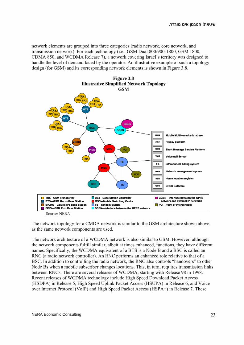
network elements are grouped into three categories (radio network, core network, and transmission network). For each technology (i.e., GSM Dual 800/900-1800, GSM 1800, CDMA 850, and WCDMA Release 7), a network covering Israel’s territory was designed to handle the level of demand faced by the operator. An illustrative example of such a topology design (for GSM) and its corresponding network elements is shown in Figure 3.8.
Figure 3.8 Illustrative Simplified Network Topology
GSM
TRX—GSM TransceiverBTS—GSM Macro Base StationMICRO—GSM Micro Base StationPICO—GSM Pico Base Station
BSc—Base Station ControllerMSC—Mobile Switching CentreTS—Tandem SwitchSGSN—interface between the GPRS network
GGSN—interface between the GPRS network and external IP networks
POI—Point of interconnect
MSC
BTS
POI
Prepay platform
Short Message Service Platform
Mobile Multi—media database
Voicemail Server
Interconnect billing system
Network management system
Home location register
TRXTRX TRX
TRXTRX TRX
BTS
TRXTRX TRX TRX
TRX TRXTRX
TRX TRX
SGSN
MSC
TS
PRP
SMS
MMS
VMS
BIL
NMS
HLR
GPR GPRS Software
TRXTRX
TRX
PICO POI
TSBSC
MICRO
BSCGGSN
TRX—GSM TransceiverBTS—GSM Macro Base StationMICRO—GSM Micro Base StationPICO—GSM Pico Base Station
BSc—Base Station ControllerMSC—Mobile Switching CentreTS—Tandem SwitchSGSN—interface between the GPRS network
GGSN—interface between the GPRS network and external IP networks
POI—Point of interconnect
MSC
BTS
POI
Prepay platform
Short Message Service Platform
Mobile Multi—media database
Voicemail Server
Interconnect billing system
Network management system
Home location register
TRXTRX TRX
TRXTRX TRX
BTS
TRXTRX TRX TRX
TRX TRXTRX
TRX TRX
SGSN
MSC
TS
PRP
SMS
MMS
VMS
BIL
NMS
HLR
GPR
PRP
SMS
MMS
VMS
BIL
NMS
HLR
GPR GPRS Software
TRXTRX
TRX
PICO POI
TSBSC
MICRO
BSCGGSN
Source: NERA
The network topology for a CMDA network is similar to the GSM architecture shown above, as the same network components are used.
The network architecture of a WCDMA network is also similar to GSM. However, although the network components fulfill similar, albeit at times enhanced, functions, they have different names. Specifically, the WCDMA equivalent of a BTS is a Node B and a BSC is called an RNC (a radio network controller). An RNC performs an enhanced role relative to that of a BSC. In addition to controlling the radio network, the RNC also controls “handovers” to other Node Bs when a mobile subscriber changes locations. This, in turn, requires transmission links between RNCs. There are several releases of WCDMA, starting with Release 98 in 1998. Recent releases of WCDMA technology include High Speed Download Packet Access (HSDPA) in Release 5, High Speed Uplink Packet Access (HSUPA) in Release 6, and Voice over Internet Protocol (VoIP) and High Speed Packet Access (HSPA+) in Release 7. These

.הסגנון אינו מוגדר! שגיאה
NERA Economic Consulting 24
later releases require upgrades to the RNCs and Node Bs. These upgrade costs are reflected in the cost model.
Although Releases 8, 9, and 10 are at various stages of the development process, the NERA BU-LRIC model dimensions WCDMA networks for Release 7. We find this to be the appropriate technology and architecture modeling choice for Israel for several reasons. First, in their submissions, the Israeli MNOs state that WCDMA Release 7 is scheduled to be deployed in 2010. Hence, it represents a forward-looking technology, consistent with the model’s objective. Second, given the continued uncertainty in the industry over Release 8 and later releases, it appears premature (and consequently controversial) to derive cost and performance estimates for these releases. Finally, the Israeli MNOs also have indicated a preference to deploy Release 10 (LTE) when it becomes available.17
3.2.1 Model geotypes
In order to tailor the modeled networks to the different levels of demand in varied geographic areas, the NERA BU-LRIC model categorizes the demand according to traffic densities in different areas (known as geotypes). The geotype information provided by the operators is shown in Table 3.7 below.
Table 3.7 Geotype Characteristics
Cellcom Partner Pelephone
Geotype Area (sq. km)
Population Area (sq. km)
Population Area (sq. km)
Population
Dense Urban - - - - 158 -
Urban 1,857 5,990,580 1,824 5,972,000 4,698 -
Suburban 3,153 836,510 24,619 1,493,000 2,844 -
Rural 16,650 18,250 - - 19,034 -
Deserted - - 1,410 - 885 -
Total 21,659 6,845,340 27,853 7,465,000 27,619 - Source: Operator submissions Note: “-” denotes no data submitted.
As can be seen, the three operators seem to have relied on different definitions of geotypes. Cellcom divided its serving area into three categories (urban, suburban, and rural), Partner used three differently defined categories of geotype (urban, suburban, deserted), and Pelephone used five geotypes. Cellcom’s data were problematic in that the area figures appeared to exclude the West Bank, although other data from Cellcom did not. Similarly, Partner’s data were difficult to incorporate as no information was provided about rural areas. Hence, we opted to rely on
17 LTE is a mobile communication system that is an evolution of the GSM and UMTS systems. It is still a 3G technology. LTE Advanced is a 4G technology.

.הסגנון אינו מוגדר! שגיאה
NERA Economic Consulting 25
Pelephone’s data, combining “dense urban” and “urban” into one geotype. The resulting geotype data, which are used in the model, are shown in Table 3.8 below. We note that, although deserted areas are taken into account, the model does not dimension for these areas as there is no traffic in this geotype.
Table 3.8 Geotype Data Used in Model
Area (km) % of Total Area % of Annual Traffic
Urban 4,856 17.6% 81.7%
Suburban 2,844 10.3% 6.8%
Rural 19,034 68.9% 11.5%
Deserted 885 3.2% 0.0%
Total 27,619 100.0% 100.0% Source: NERA analysis based on operator submissions
The size of the network in each geotype is determined by one of two drivers. Either the dimensioning is based on the coverage requirement (i.e., the number of BTSs required to provide geographic coverage), or the size is determined by the network traffic in the area (i.e., the network must provide a given level of traffic capacity for a given level of utilization).
3.2.2 Dimensioning assumptions
Network dimensioning starts with estimating the radio network required to handle demand. We assume three different cell types: macrocells, microcells, and picocells. Although the area that can be covered by each cell type depends on the immediate environment, macrocells have the largest cell radius, followed by microcells, and then picocells. For macrocells, the base station antennas are installed on a mast (greenfield) or on top of a tall building. Microcells require lower antenna heights and are typically used in urban settings. Finally, a picocell is designed to serve a very small area, such as part of a building, a street corner, or an airplane cabin. They can be used to extend coverage to indoor areas that are inaccessible to outdoor signals or to add network capacity in areas with very dense phone usage.
The objective of the model is to design a radio network configuration that meets the required level of demand. To do this, we incorporated the following assumptions in the model:
A network is rolled out to provide geographical coverage (i.e., there is only a minimum level of traffic).
Each coverage base station contains one sector, and there is a minimum of one transceiver per sector.
The minimum transceiver configuration of a macro base station is one transceiver per sector.

.הסגנון אינו מוגדר! שגיאה
NERA Economic Consulting 26
To accommodate traffic, MNOs usually have to split sites into several smaller areas to handle the density of traffic. The model tracks that process by employing the cell radii that the MNOs in Israel have found to be necessary, thus providing enough cell sites to handle the traffic. This approach has the additional benefit that the particular mix of terrain and buildings in Israel is reflected in the cell radii actually employed by the operators.
Transceivers are added to each base station in response to traffic demand until each base station is fully configured.
In the dual band networks, such as GSM 900-1800 or WCDMA 850-2100, transceivers for each band are colocated at the same base stations and additional GSM 1800 transceivers (or WCDMA 850 and 2100 transceivers) and equipment are added to provide additional traffic capacity.
Once each base station is fully configured with both GSM 900 and GSM 1800 transceivers (or WCDMA 850 and 2100 transceivers), additional base stations are added to provide additional traffic capacity.
The upper limit on the number of transceivers per base station is determined by either:
− The physical limit of the number of transceivers, which is a maximum of six transceivers per sector.
− The number of transceivers per sector that the spectrum will allow—the model derives this from the spectrum allocations and, for bands that can be used for both 2G and 3G (such as 850), after allowing for any allocation to either 2G or 3G.
2G and 3G networks for each existing MNO are modeled as if it was entering the market now at its current scale and scope of operation with either a single 3G network or both a 2G and 3G network.
3.2.3 Minimum coverage network
Based on these assumptions, the model derives a minimum coverage network. Specifically, it determines the number of base stations required to provide coverage to the area and the minimum amount of network equipment required to enable a voice call to be conveyed between any two points in the coverage area. It is important to note that the costs of the minimum coverage network are a network common cost (i.e., the minimum coverage network is required whichever services are provided. Its annualized cost is calculated and treated as a markup on the LRIC costs of the traffic network. A summary of the volumes of network elements required for the minimum coverage network for Cellcom’s GSM 1800 network is shown in Table 3.9.

.הסגנון אינו מוגדר! שגיאה
NERA Economic Consulting 27
Table 3.9 Minimum Coverage Network
Example of Cellcom GSM 1800
Network Element 2009 2010 2011 2012 2013 2014
BTS 553 553 553 553 553 553
BSC 2 2 2 2 2 2
MSC 1 1 1 1 1 1
HLR 1 1 1 1 1 1
TS 1 1 1 1 1 1 Source: NERA calculations Note: These values depend on the scenario chosen.
We also include an interconnection billing system, a point of interconnection, and spectrum license fees in the definition of the minimum coverage network, as these are required to provide voice services. The minimum network definition excludes the provision of prepaid, SMS, and GPRS data services because they would not be provided as part of the minimum coverage network requirement.
3.2.4 Traffic network
While the minimum coverage network determines the common cost component, the traffic network determines the incremental costs.
3.2.4.1 Cell radii and base station types
The cell radii for the traffic network in the NERA BU-LRIC model are summarized in Table 3.10.
Table 3.10 Cell Radii for Traffic Base Stations (km)
Geotype 2G
CDMA 850
2G GSM 900
2G GSM 1800
3G WCDMA
850
3G WCDMA
900
3G WCDMA
2100
Urban 1.5 1.5 1.5 1.5 1.5 1.3
Suburban 2.2 3.5 3.5 2.2 2.2 1.8
Rural 4.3 4.0 4.0 4.3 4.3 3.6
Highway/Railway 2.2 3.5 3.5 2.2 2.2 1.8
Tunnel etc 1.5 1.5 1.5 1.5 1.5 1.3 Source: NERA analysis
Unlike in the case of a minimum coverage network, the traffic network also includes microcells and in-building base stations. However, these are deployed only in urban and suburban areas.

.הסגנון אינו מוגדר! שגיאה
NERA Economic Consulting 28
We dimension the amount of traffic carried by these base stations using information in the operators’ submissions. As Pelephone did not provide any data in response to this request, we used for Pelephone the data provided by Partner as these data were most complete.
Table 3.11 Traffic Carried Using Micro- and Picocells
Operator Technology Microcell Picocell
2G 3% n/a Cellcom
3G 3% n/a
2G 2% 5% Partner
3G 0% 4%
2G - - Pelephone
3G - - Source: Operator submissions Note: “-” denotes no data submitted.
The proportion of different cell-site types and the way in which the equipment is mounted differs by operator. For Cellcom and Partner, the distribution of cell-site types relies on the carriers’ respective data declarations. Pelephone did not submit any data. Consequently, Pelephone’s cell-type mix is based on data received from the Ministry of Environmental Protection, which lists all cell sites in Israel based on cell-site type.
The NERA model also allows for areas of special coverage, specifically along highways or railways and in tunnels, underground, subway or metro systems. Data in response to NERA’s request on this point were received from Cellcom and Partner. However, the Cellcom “Highway/Railway” figures appeared anomalously high, so we have used those from Partner instead. Conversely, Partner provided no “Tunnel/Subway/Underground/Metro” data, so we have relied on the Cellcom figures.
Table 3.12 Special coverage
Type Coverage (km)
Highway/Railway 26
Tunnel/Subway/Underground/Metro 100 Source: NERA
3.2.4.2 Traffic capacity calculation
The traffic capacity required by each base station is determined using an Erlang B table. An Erlang is a unit of telecommunications traffic measurement, which represents the continuous use of one voice path (and thus the related traffic volume) for one hour. Erlang traffic measurements or estimates can be used to work out how many circuits are required between

.הסגנון אינו מוגדר! שגיאה
NERA Economic Consulting 29
different parts of a network or between multiple network locations. The traffic capacity (as shown in the Erlang B table) is a function of:
The number of transceivers deployed in each base station sector
The number of traffic channels per transceiver
The level of call blocking in the radio network
The model includes an assumed blocking probability of 1 percent (or P=.01) for 2G and 3G networks. This is consistent with the data submission from Cellcom and general engineering standards. An example of this traffic dimensioning calculation is shown in Figure 3.9 below.
Figure 3.9 Traffic Dimensioning Calculation
# transceivers per sector
e.g. 3 to provide maximumcapacity on the network
within the spectrum allocation
# transceivers per sector
e.g. 3 to provide maximumcapacity on the network
within the spectrum allocation
Number of channelper sector
e.g. 207
Number of channelper sector
e.g. 207
# channels per transceiver
Set to 69 channels per 3G transceiver
[typical value for WCDMA]
# channels per transceiver
Set to 69 channels per 3G transceiver
[typical value for WCDMA]
Level of radio network blocking
e.g. 1%[% of calls that cannot be made
because a radio channelis not available]
Level of radio network blocking
e.g. 1%[% of calls that cannot be made
because a radio channelis not available]
Erlangs per sectore.g. each sector can carry
184.6 Erlangs of traffic
The Erlang table is used tocalculate the amount of
traffic that can be carried byeach sector
Erlangs per sectore.g. each sector can carry
184.6 Erlangs of traffic
The Erlang table is used tocalculate the amount of
traffic that can be carried byeach sector
Erlang table look-up
# transceivers per sector
e.g. 3 to provide maximumcapacity on the network
within the spectrum allocation
# transceivers per sector
e.g. 3 to provide maximumcapacity on the network
within the spectrum allocation
Number of channelper sector
e.g. 207
Number of channelper sector
e.g. 207
# channels per transceiver
Set to 69 channels per 3G transceiver
[typical value for WCDMA]
# channels per transceiver
Set to 69 channels per 3G transceiver
[typical value for WCDMA]
Level of radio network blocking
e.g. 1%[% of calls that cannot be made
because a radio channelis not available]
Level of radio network blocking
e.g. 1%[% of calls that cannot be made
because a radio channelis not available]
Erlangs per sectore.g. each sector can carry
184.6 Erlangs of traffic
The Erlang table is used tocalculate the amount of
traffic that can be carried byeach sector
Erlangs per sectore.g. each sector can carry
184.6 Erlangs of traffic
The Erlang table is used tocalculate the amount of
traffic that can be carried byeach sector
Erlang table look-up
Source: NERA
Figure 3.9 illustrates how the NERA BU-LRIC model dimensions the traffic on one base station sector. In this example, there are three transceivers per sector. Each WCDMA transceiver on a sector can be configured for 69 voice channels. For three transceivers, there are 207 (69 x 3) channels available to accommodate the traffic. Using a blocking probability of 1 percent, the Erlang table indicates that with 207 channels, 184.6 Erlangs of traffic can be carried by the sector. As illustrated in this example, the capacity (Erlangs per sector) also depends on the number of transceivers per sector. This, in turn, is calculated using:
The level of traffic capacity required
The traffic capacity provided by the traffic network
The cap on the number of transceivers per base station resulting from either the amount of available spectrum or the physical capacity per sector (which varies depending on the technology employed)

.הסגנון אינו מוגדר! שגיאה
NERA Economic Consulting 30
The Erlang look-up table that provides the amount of traffic that can be handled for a given blocking probability and the number of available channels is based upon statistical engineering calculations. An excerpt from it is shown in Table 3.13 below.
Table 3.13 Excerpt of Erlang Lookup Table
Blocking Probabilities Channels
0.10% 0.50% 1% 2% 3% 5% 10%
0 0.00 0.00 0.00 0.00 0.00 0.00 0.00
1 0.00 0.01 0.01 0.02 0.03 0.05 0.11
2 0.05 0.11 0.15 0.22 0.28 0.38 0.60
3 0.19 0.35 0.46 0.60 0.72 0.90 1.27
4 0.44 0.70 0.87 1.09 1.26 1.52 2.05 Source: ITU
3.2.4.3 Spectrum reuse patterns
Before the traffic network can be dimensioned, it is necessary to determine not only the cell radius but also the frequency reuse pattern in the case of multifrequency networks, such as GSM. In contrast to a network with a single transmitter, a cellular network has multiple transmitters and thus the ability to reuse the same frequency in a different area. This increases the capacity in a cellular network because many subscribers can use a single frequency. In order to minimize the level of interference from reusing the same frequency, a frequency reuse pattern must be established. The frequency reuse pattern sets an upper limit on the number of transceivers that a base station sector can operate for a given amount of spectrum. This, in turn, influences the number of base stations in the network. It should be noted that WCDMA operates as a single frequency network (SFN), where each base station operates at the same frequency (or frequencies) as its neighbors; in this case, frequency reuse is 100 percent.
To determine the reuse pattern, the coverage area is depicted as a series of contiguous hexagons. Each hexagon represents the serving area of a base station, which is split into three sectors. As shown in Figure 3.10, we assume a frequency reuse pattern of 12 for GSM, which allows there to be at least one sector gap between cells that use the same frequency. This is equivalent to a base station frequency reuse of four (assuming three sectors per base station).
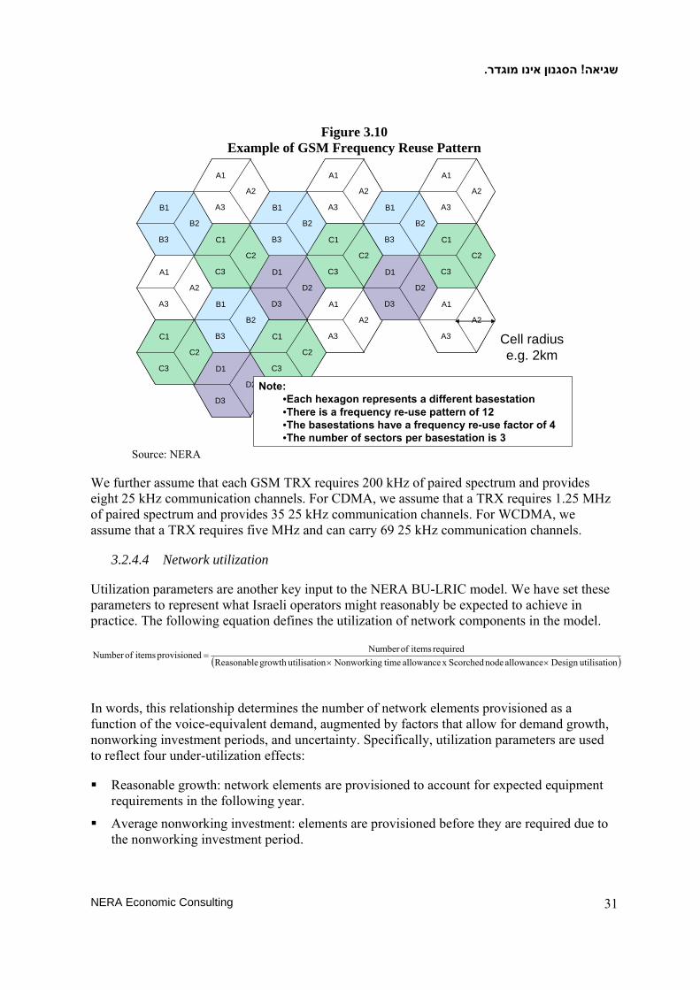
.הסגנון אינו מוגדר! שגיאה
NERA Economic Consulting 31
Figure 3.10 Example of GSM Frequency Reuse Pattern
A1
A2
A3
A1
A2
A3
D1
D2
D3
D1
D2
D3B1
B2
B3
B1
B2
B3
D1
D2
D3
D1
D2
D3
A1
A2
A3
A1
A2
A3 B1
B2
B3
B1
B2
B3 C1
C2
C3
C1
C2
C3
A1
A2
A3
A1
A2
A3
C1
C2
C3
C1
C2
C3
C1
C2
C3
C1
C2
C3
A1
A2
A3
A1
A2
A3
C1
C2
C3
C1
C2
C3
B1
B2
B3
B1
B2
B3
D1
D2
D3
D1
D2
D3
C1
C2
C3
C1
C2
C3
B1
B2
B3
B1
B2
B3
A1
A2
A3
A1
A2
A3
A1
A2
A3
A1
A2
A3
Cell radiuse.g. 2km
Note: •Each hexagon represents a different basestation•There is a frequency re-use pattern of 12•The basestations have a frequency re-use factor of 4•The number of sectors per basestation is 3
Source: NERA
We further assume that each GSM TRX requires 200 kHz of paired spectrum and provides eight 25 kHz communication channels. For CDMA, we assume that a TRX requires 1.25 MHz of paired spectrum and provides 35 25 kHz communication channels. For WCDMA, we assume that a TRX requires five MHz and can carry 69 25 kHz communication channels.
3.2.4.4 Network utilization
Utilization parameters are another key input to the NERA BU-LRIC model. We have set these parameters to represent what Israeli operators might reasonably be expected to achieve in practice. The following equation defines the utilization of network components in the model.
( )nutilisatioDesignallowancenodeScorched x allowance timeNonworkingnutilisatiogrowth ReasonablerequireditemsofNumber
dprovisioneitemsofNumber××
=
In words, this relationship determines the number of network elements provisioned as a function of the voice-equivalent demand, augmented by factors that allow for demand growth, nonworking investment periods, and uncertainty. Specifically, utilization parameters are used to reflect four under-utilization effects:
Reasonable growth: network elements are provisioned to account for expected equipment requirements in the following year.
Average nonworking investment: elements are provisioned before they are required due to the nonworking investment period.
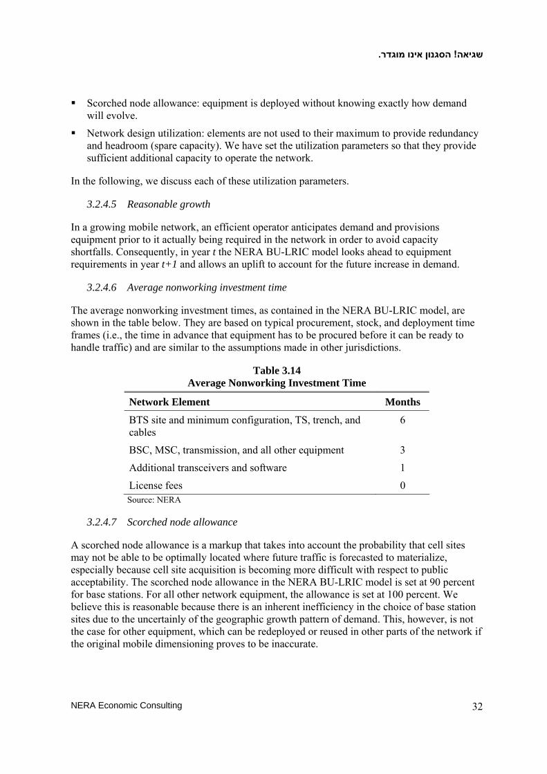
.הסגנון אינו מוגדר! שגיאה
NERA Economic Consulting 32
Scorched node allowance: equipment is deployed without knowing exactly how demand will evolve.
Network design utilization: elements are not used to their maximum to provide redundancy and headroom (spare capacity). We have set the utilization parameters so that they provide sufficient additional capacity to operate the network.
In the following, we discuss each of these utilization parameters.
3.2.4.5 Reasonable growth
In a growing mobile network, an efficient operator anticipates demand and provisions equipment prior to it actually being required in the network in order to avoid capacity shortfalls. Consequently, in year t the NERA BU-LRIC model looks ahead to equipment requirements in year t+1 and allows an uplift to account for the future increase in demand.
3.2.4.6 Average nonworking investment time
The average nonworking investment times, as contained in the NERA BU-LRIC model, are shown in the table below. They are based on typical procurement, stock, and deployment time frames (i.e., the time in advance that equipment has to be procured before it can be ready to handle traffic) and are similar to the assumptions made in other jurisdictions.
Table 3.14 Average Nonworking Investment Time
Network Element Months
BTS site and minimum configuration, TS, trench, and cables
6
BSC, MSC, transmission, and all other equipment 3
Additional transceivers and software 1
License fees 0 Source: NERA
3.2.4.7 Scorched node allowance
A scorched node allowance is a markup that takes into account the probability that cell sites may not be able to be optimally located where future traffic is forecasted to materialize, especially because cell site acquisition is becoming more difficult with respect to public acceptability. The scorched node allowance in the NERA BU-LRIC model is set at 90 percent for base stations. For all other network equipment, the allowance is set at 100 percent. We believe this is reasonable because there is an inherent inefficiency in the choice of base station sites due to the uncertainly of the geographic growth pattern of demand. This, however, is not the case for other equipment, which can be redeployed or reused in other parts of the network if the original mobile dimensioning proves to be inaccurate.
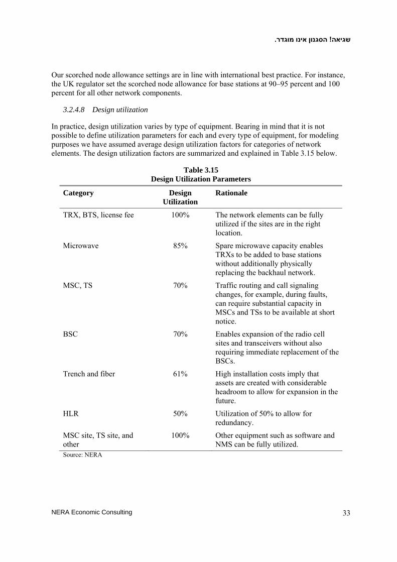
.הסגנון אינו מוגדר! שגיאה
NERA Economic Consulting 33
Our scorched node allowance settings are in line with international best practice. For instance, the UK regulator set the scorched node allowance for base stations at 90–95 percent and 100 percent for all other network components.
3.2.4.8 Design utilization
In practice, design utilization varies by type of equipment. Bearing in mind that it is not possible to define utilization parameters for each and every type of equipment, for modeling purposes we have assumed average design utilization factors for categories of network elements. The design utilization factors are summarized and explained in Table 3.15 below.
Table 3.15 Design Utilization Parameters
Category Design Utilization
Rationale
TRX, BTS, license fee 100% The network elements can be fully utilized if the sites are in the right location.
Microwave 85% Spare microwave capacity enables TRXs to be added to base stations without additionally physically replacing the backhaul network.
MSC, TS 70% Traffic routing and call signaling changes, for example, during faults, can require substantial capacity in MSCs and TSs to be available at short notice.
BSC 70% Enables expansion of the radio cell sites and transceivers without also requiring immediate replacement of the BSCs.
Trench and fiber 61% High installation costs imply that assets are created with considerable headroom to allow for expansion in the future.
HLR 50% Utilization of 50% to allow for redundancy.
MSC site, TS site, and other
100% Other equipment such as software and NMS can be fully utilized.
Source: NERA

.הסגנון אינו מוגדר! שגיאה
NERA Economic Consulting 34
3.3 Switching
3.3.1 Second generation networks
With the radio network dimensioned, this section explains how the model dimensions the transmission and switching networks. Figure 3.11 illustrates the assumed backhaul transmission network architecture for 2G networks. It includes both tandem and mobile switching layers. The points of interconnection are situated at both the MSC and TS layer.
Figure 3.11 2G Transmission and Switching Network Topology
TS TS
MSC MSC MSC
BSCBSCBSC
POI
POI POI
BSC layer
Mobile switching layer
Tandem switching layer
Source: NERA
Below, we describe the dimensioning of each of these elements.
Base station controllers: The dimensioning of the radio network results in the number of required TRXs. This in turn determines the number of BSCs, as each BSC can only support a finite number of TRXs. Specifically, we assume that a BSC can control up to 512 GSM TRXs. We further assume that BSCs are colocated with mobile switching centers and tandem switches.
Mobile switching centers: The number of MSCs is determined by BHCAs and the BHCA capacity of each MSC. The capacity of an MSC to handle BHCAs has been taken from the submission from Cellcom, which explains that its MSCs on average have a BHCA capacity of 800,000.
Tandem Switching: In order to dimension the number of TSs, NERA has estimated the number of TSs as a proportion of the number of MSCs in each network. We have used the operators’ actual ratios of MSCs to TSs to estimate these proportions, except in the case of Pelephone. For Pelephone, which did not provide data in response to NERA’s data request on this point, we used data from the other Israeli operators.

.הסגנון אינו מוגדר! שגיאה
NERA Economic Consulting 35
3.3.2 Third generation networks
Figure 3.12 below illustrates the backhaul transmission network that we have assumed for 3G networks. It includes both tandem and mobile switching layers. The points of interconnection are situated at both the MSC and TS layers.
Figure 3.12 3G Transmission and Switching Network Topology
TS TS
MSC MSC MSC
RNC RNC
POI
POI POI
RNC layer
Mobile switching layer
Tandem switching layer
RNC
Source: NERA
The dimensioning of switching in the 3G networks follows the same logic and assumptions as those used in the 2G networks.
3.3.3 Transmission
We have implemented three forms of transmission in the model, namely: leased lines, microwave, and (self provided) fixed lines.
Cellcom and Partner provided information on self-provided transmission equipment, and this “MNO specific” data can be selected in the model using the switches in cells C24 and C25 of the “Inputs” sheet. However, according to the LRIC approach, the least-cost asset should be adopted, which we believe is microwave equipment for BTS-BSC and Node B-RNC links and leased lines for other transmission links. The capacity deployed is determined by the estimated capacity required in 2009 in the 2G networks and the capacity required in 2014 in the 3G networks. The reason for this is that 2G traffic volumes fall over time and 3G traffic volumes increase over time because of the shift from 2G to 3G. Consequently, we dimension the transmission capacity to handle the maximum traffic volumes predicted by the model.

.הסגנון אינו מוגדר! שגיאה
NERA Economic Consulting 36
3.3.3.1 Leased lines
Leased lines are assumed to be available in the following capacity units: E1, E2, E3, STM-1, and STM-16. Based on operator submissions for BSC-SGSN, SGSN-GGSN, and RNC-RNC links, the model accommodates the use of Ethernet leased lines. Leased line costs were modeled based on the leased line prices offered by Bezeq. We assume that these prices remain constant in real terms per annum and note that they are not distance dependent. Table 3.16 below illustrates a selection of the figures used in the model.
Table 3.16 Leased Line Charges in 2009
(ILS per annum)
Distance E1 E2 E3 STM-1 STM-4 STM-16 GbE
1 km 13,152 37,000 102,000 174,000 294,000 497,000
10 km 13,152 37,000 102,000 174,000 294,000 497,000
49 km 13,152 37,000 102,000 174,000 294,000 497,000
199 km 13,152 37,000 102,000 174,000 294,000 497,000
499 km 13,152 37,000 102,000 174,000 294,000 497,000 Source: NERA analysis based on Bezeq data received from the MOC.
3.3.3.2 Microwave
Microwave units are assumed to be available in the following capacity units: E1, E2, E3, STM-1, and STM-16. A multi-hop factor is applied to arrive at the number of microwave units required to provide a link of the required distance. The multi-hop factor is based upon the range of the technology (assumed to be 40 km) and the distance of each of the transmission links. The average transmission lengths are based on the distances implied by the geographic coverage area of each unit of network equipment. Table 3.17 shows the estimates using the example of Pelephone.

.הסגנון אינו מוגדר! שגיאה
NERA Economic Consulting 37
Table 3.17 Pelephone Modeled Average Transmission Lengths
(2009, km)
Link type Average distance, km
BTS-BSC* 34
RNC-RNC NA (GbE standard tariff)
BSC-MSC** 34
MSC-MSC 34
MSC-TS*** 49
TS-TS 0
BSC-SGSN 45
SGSN-GGSN NA (GbE standard tariff) Source: NERA Notes: * microwave links only; ** if the BSC is collocated with the MSC, this is assumed to be zero; *** assumed to be zero due to colocation.
3.3.4 Other network elements
The derivation of the capacity required for other network elements is provided in the detailed technical documentation of the model.
3.4 Network Sharing
The model takes into account two forms of network sharing: sharing within a network of 2G and 3G assets and the sharing of sites between operators.
3.4.1 2G/3G sharing
Network assets that could be shared between 2G and 3G services include:
BTS/Node B sites
MSC sites (which also house most BSCs and RNCs)
MSC equipment (vendors can provide switches to handle both 2G and 3G traffic and signaling)
3.4.2 Operator site sharing
The model can take into account BTS/Node B site sharing between operators. Information from the MOC suggests that up to 20 percent of any operator’s sites can be shared. When the cost of these sites is shared equally with another operator, the effect is that an operator pays the full cost for only 80 percent of its sites and half the cost of the other 20 percent of its sites, resulting in a cost of only 90 percent of the total costs of the sites.

.ן אינו מוגדרהסגנו! שגיאה
NERA Economic Consulting 38
3.5 Network Asset Valuation
Having established the required quantities of network equipment, the model calculates the associated capital expenditures by applying MEA unit costs (in Israeli shekels) along with price trends. We also add an allowance for indirect network assets such as buildings, vehicles, computers, and office equipment.
3.5.1 Asset unit costs
The asset “unit costs” (i.e., prices paid for equipment) represent the 2009 MEA value expressed in Israeli shekels. A full list of these input prices is contained in the NERA BU-LRIC model in tab “1 Inputs” starting with row 749. The asset unit costs were derived based on limited cost data received from the Israeli operators and cost data incorporated in mobile LRIC models for other countries. Specifically, we relied on cost data received from MIRS, Pelephone, and Cellcom. No cost data were provided by Partner. Where cost data were not provided, we relied on average cost data incorporated in mobile LRIC models in two other countries (UK and France), the previous Israeli LRIC model, as well as our experience from other countries. We note that, where we had to rely on cost information provided in the past (i.e., previous cost models), we used the 2009 forecasted asset prices from those models.
We derived the final asset unit cost estimates by taking a simple average of all data points collected. For all assets for which we received cost information from at least one Israeli operator, we used the average of these Israeli numbers instead of the international average.
3.5.2 MEA price trends
No Israeli operator provided MEA price trends. Hence, we relied on the same data sources as described above and derived an international average. The model does not reflect possible changes in the value of the Israeli shekel during the study period relative to other currencies.
3.5.3 Network operating costs
In the absence of data from the operators, we based network operating costs on the same methodology described above. Operating expenses are calculated as the sum of direct and indirect operating expenses.
3.5.4 Indirect network assets
We add indirect network assets to the value of the direct network investment. These assets comprise nonoperational buildings (i.e., buildings that do not form part of the network but are used by network employees), vehicles, general purpose computers, and office and other equipment. In the absence of information in the requested form from the operators, the amounts are based upon NERA’s experience from previous cost modeling exercises and are shown in Table 3.18 below.
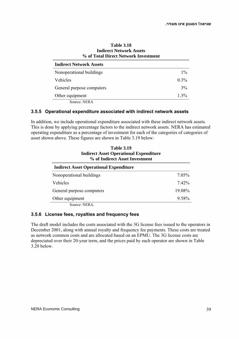
.הסגנון אינו מוגדר! שגיאה
NERA Economic Consulting 39
Table 3.18 Indirect Network Assets
% of Total Direct Network Investment
Indirect Network Assets
Nonoperational buildings 1%
Vehicles 0.3%
General purpose computers 3%
Other equipment 1.3% Source: NERA
3.5.5 Operational expenditure associated with indirect network assets
In addition, we include operational expenditure associated with these indirect network assets. This is done by applying percentage factors to the indirect network assets. NERA has estimated operating expenditure as a percentage of investment for each of the categories of categories of asset shown above. These figures are shown in Table 3.19 below:
Table 3.19 Indirect Asset Operational Expenditure
% of Indirect Asset Investment
Indirect Asset Operational Expenditure
Nonoperational buildings 7.05%
Vehicles 7.42%
General purpose computers 19.08%
Other equipment 9.58% Source: NERA.
3.5.6 License fees, royalties and frequency fees
The draft model includes the costs associated with the 3G license fees issued to the operators in December 2001, along with annual royalty and frequency fee payments. These costs are treated as network common costs and are allocated based on an EPMU. The 3G license costs are depreciated over their 20-year term, and the prices paid by each operator are shown in Table 3.20 below.
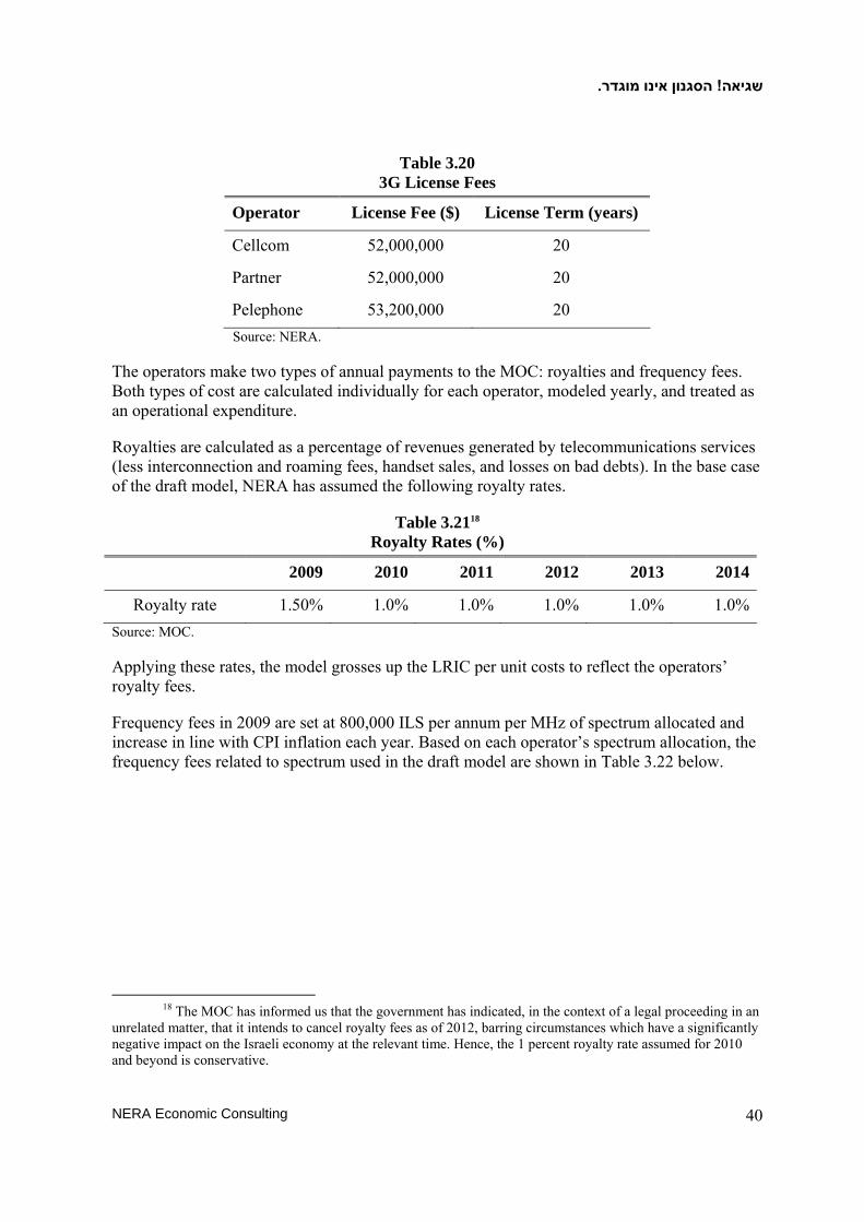
.הסגנון אינו מוגדר! שגיאה
NERA Economic Consulting 40
Table 3.20 3G License Fees
Operator License Fee ($) License Term (years)
Cellcom 52,000,000 20
Partner 52,000,000 20
Pelephone 53,200,000 20 Source: NERA.
The operators make two types of annual payments to the MOC: royalties and frequency fees. Both types of cost are calculated individually for each operator, modeled yearly, and treated as an operational expenditure.
Royalties are calculated as a percentage of revenues generated by telecommunications services (less interconnection and roaming fees, handset sales, and losses on bad debts). In the base case of the draft model, NERA has assumed the following royalty rates.
Table 3.2118 Royalty Rates (%)
2009 2010 2011 2012 2013 2014
Royalty rate 1.50% 1.0% 1.0% 1.0% 1.0% 1.0%Source: MOC.
Applying these rates, the model grosses up the LRIC per unit costs to reflect the operators’ royalty fees.
Frequency fees in 2009 are set at 800,000 ILS per annum per MHz of spectrum allocated and increase in line with CPI inflation each year. Based on each operator’s spectrum allocation, the frequency fees related to spectrum used in the draft model are shown in Table 3.22 below.
18 The MOC has informed us that the government has indicated, in the context of a legal proceeding in an
unrelated matter, that it intends to cancel royalty fees as of 2012, barring circumstances which have a significantly negative impact on the Israeli economy at the relevant time. Hence, the 1 percent royalty rate assumed for 2010 and beyond is conservative.

.הסגנון אינו מוגדר! שגיאה
NERA Economic Consulting 41
Table 3.22 Spectrum Frequency Fees (ILS)
2009 2010 2011 2012 2013 2014
Cellcom 17,600,000 18,121,695 18,564,600 9,540,357 9,773,772 10,011,858 Partner 27,200,000 28,006,257 28,690,745 29,488,375 30,209,841 30,945,744
2G
Pelephone 32,640,000 33,607,508 34,428,894 17,346,103 17,770,495 18,203,379 Cellcom 16,000,000 16,474,269 16,876,909 26,886,460 27,544,266 28,215,237 Partner 32,000,000 32,948,537 33,753,817 34,692,206 35,540,989 36,406,757
3G
Pelephone 16,000,000 16,474,269 16,876,909 35,386,050 36,251,809 37,134,892 Source: MOC and NERA calculations
In addition to the frequency fees, the operators make additional payments for microwave frequencies. The MOC has provided NERA with information on the 2009 microwave frequency fees paid by the operators and the corresponding numbers of links. From these, NERA has calculated an average fee per link (4,963 ILS in 2009) and multiplied this by the relevant numbers of links in each 2G and 3G network in the model. Microwave frequency fees are assumed to increase in line with the CPI in the same manner that spectrum frequency fees do.
3.6 Capital Charge Determination
3.6.1 Depreciation method
Once the total investment for the hypothetical, efficient, least-cost carrier with the same scale and scope of operations as the relevant actual Israeli operator has been determined, the model calculates the annualized capital charge as a percentage of investment by applying an appropriate depreciation method and the cost of capital (CoC). While we generally agree that the model should rely on economic depreciation, there are a variety of problems with its implementation—one of which is the need to forecast prices, output, and operating expenses into the distant future. Hence, the NERA BU-LRIC model currently only offers the choice of several accounting depreciation methods. However, the user can choose a method that likely approximates economic depreciation. Specifically, the NERA BU-LRIC model incorporates the following depreciation methods:
Straight-line depreciation: Under this method, assets are depreciated by a constant amount each year over their lifetimes (i.e., there is a flat depreciation schedule). The annual capital charge is:
Investment cost x (1/asset life + CoC).
Although it is a clear-cut method, straight-line depreciation has been criticized for not accurately approximating economic depreciation and for possibly leading to imperfect cost recovery in situations where asset prices change over the economic life of the asset.
Tilted straight line: Using this method, assets are depreciated each year by the current price of a new asset divided by the asset life plus a term that takes into account the change in asset price over the year. The annual capital charge in the first year is:

.הסגנון אינו מוגדר! שגיאה
NERA Economic Consulting 42
Investment cost x {(1 + annual % price change) x [1/asset life – annual % price change * remaining asset life/ asset life]} + Investment cost * CoC.
The slope of the depreciation schedule therefore depends on whether and by how much prices change.
Sum-of-the-years digits: Under this depreciation method, the annual depreciation expense is a fraction with a numerator equal to the remaining years of economic life and the denominator is equal to the sum-of-the-years of economic life. It is best demonstrated with the aid of an example:
Suppose an asset has a 10-year life. The sum-of-the-years digits is equal to 1 + 2 + 3+ … + 10 = 55. In the first year, depreciation is 10/55 of the asset value, in the second year 9/55, in the third year 8/55, and so on. As can be seen, this results in a downward sloping depreciation schedule over time.
Annuity: A normal annuity implies a constant payment covering depreciation and the cost of capital in each year of the asset’s life. At the start, this payment consists more of the cost of capital payments (for example, interest on debt) and less of depreciation costs. Towards the end of the asset life, a higher proportion of the payments are for depreciation costs and less for interest costs, so this method involves an upwards sloping depreciation schedule over time. The annual capital charge is:
Investment cost * CoC / [1-1 / (1+CoC)assetlife].
Tilted annuity: As opposed to the normal annuity explained above, a tilted annuity takes into account future trends in the price of capital equipment. Whether the depreciation schedule slopes upwards or downwards over time depends on the degree of tilt. The annual capital charge is: [Investment cost * (1+annual % price change) * (CoC- annual % price change)] / {1-[(1+annual % price change/(1+CoC)]assetlife}.
The effect of selecting different forms of depreciation is shown in sensitivity analyses presented in Appendix A.
3.6.2 Asset lives
The asset lives used in the model have been sourced from the operators’ annual reports and Form 20-F submissions. They are also consistent with NERA’s experience and assumptions in previous models. We summarize them in Table 3.23.

.הסגנון אינו מוגדר! שגיאה
NERA Economic Consulting 43
Table 3.23 Asset Lives
Asset Category Asset Life
3G license fees 20
BTS site (including installation) 15
BTS radio equipment (TRX equipment etc), BSC sites, MSC sites and TS sites (including installation), trenches and transmission cables, non-network buildings, MSC, TS, HLR, SMSC, NMS, POI, microwave links, other
10
MMSC SGSN, GGSN, transmission equipment, VMS, vehicles
7
General purpose computers 4 Sources: Israeli operator annual reports and Form 20-Fs and NERA analysis.
3.6.3 Cost of capital
NERA’s data request asked the operators for information about their cost of capital. The responses and NERA’s own estimates are shown in Table 3.24 below and detailed in Appendix C.
Table 3.24 Pretax Nominal Cost of Capital
Israeli MNO 2009
WACC Partner 9.96% Cellcom 9.37% Pelephone 9.21%
Source: NERA analysis. Note: The model uses the nominal values shown in the table as inputs and converts them to real values that are then used in the cost calculations.
The model uses the NERA estimates of pretax cost of capital for each operator, but also allows users to set their own values.
3.7 Calculation of Total LRIC
The operating costs of each network element are added to the capital charge to calculate the total cost of each network element.

.הסגנון אינו מוגדר! שגיאה
NERA Economic Consulting 44
3.8 Unit LRIC Costs
As explained above, routing factors are used to allocate costs between different services. Figure 3.13 below demonstrates the use of routing factors. We have used data submitted by the operators as the basis of the routing factors in the model and supplemented them, where necessary, with standard engineering assumptions. The detailed routing factors are contained within the model under tab “2 Routing Factor Inputs.”
Figure 3.13 Routing Factor Use
NERA BU-LRIC Model
Let:
– rik = use of network component i to produce one unit of service k
– Dk = demand for service k eg in minutes, data equivalent minutes etc
– Ci = annual cost of network component i (from previous steps)
Then:
– total use of network component i = Σ rikDk
– unit cost of network component i = Ci / Σ rikDk
– annual LRIC of service k = Σ rikDk(Ci / Σ rikDk)
Base Station (BTS)
Base Station Controller (BSC)
Mobile Switching Centre (MSC)
BTS to BSC transmission (IBT)
Call termination
On-net call Call origination
Routing factors
Costs by network element Costs by network service
Source: NERA

.הסגנון אינו מוגדר! שגיאה
NERA Economic Consulting 45
4 The Model Results
Based on the foregoing assumptions and findings, we recommend basing the LRIC cost estimates for the three operators on the following model settings:
Depreciation method: Tilted straight line
Special coverage: FALSE
Use Gigabit Ethernet (10 GbE): FALSE
Leased line discount: 0%
MNO specific backhaul (BTS): FALSE
MNO specific backhaul (Others): FALSE
Based on these settings and the given input values, the model produces LRIC estimates for voice termination, SMS, MMS, and data termination for Cellcom, Partner, and Pelephone from 2009–2014.
4.1 Voice Termination
The LRIC estimates for voice termination for Cellcom, Partner, and Pelephone are shown below. All figures are in real terms. The figure also includes the simple average cost of all three large incumbents.
Figure 4.1 NERA BU-LRIC Model Results
Per Minute Voice Termination 2G
2.0
3.0
4.0
5.0
6.0
7.0
2009 2010 2011 2012 2013 2014
Ago
rots
per
Min
ute
Cellcom Partner Pelephone Average

.הסגנון אינו מוגדר! שגיאה
NERA Economic Consulting 46
Figure 4.2
NERA BU-LRIC Model Results Per Minute Voice Termination 3G
0.0
2.0
4.0
6.0
2009 2010 2011 2012 2013 2014
Ago
rots
per
Min
ute
Cellcom Partner Pelephone Average
Table 4.1 NERA BU-LRIC Model Results Per-Minute Voice Termination
2009–2014 Voice Termination, per minute costs
2G 2009 2010 2011 2012 2013 2014Cellcom 5.03 4.29 3.98 3.81 3.69 3.78Partner 5.99 5.20 4.90 4.82 4.78 4.86Pelephone 6.18 4.92 4.45 4.12 4.20 4.45Average 5.73 4.80 4.45 4.25 4.22 4.37
3G 3.77 3.02 2.22 1.76 1.44 1.18Cellcom 4.32 2.85 2.11 1.63 1.29 1.08Partner 4.53 3.52 2.69 2.12 1.72 1.42Pelephone 4.06 3.21 2.45 1.97 1.62 1.32Average 4.30 3.19 2.42 1.90 1.54 1.27

.הסגנון אינו מוגדר! שגיאה
NERA Economic Consulting 47
4.2 SMS Termination
The LRIC estimates for SMS termination for Cellcom, Partner, and Pelephone are shown below. The figure and table also shows the simple average cost of all three large incumbents.
Figure 4.3 NERA BU-LRIC Model Results
Per SMS Termination 2G
0.0
0.2
0.4
0.6
2009 2010 2011 2012 2013 2014
Ago
rots
per
SM
S
Cellcom Partner Pelephone Average
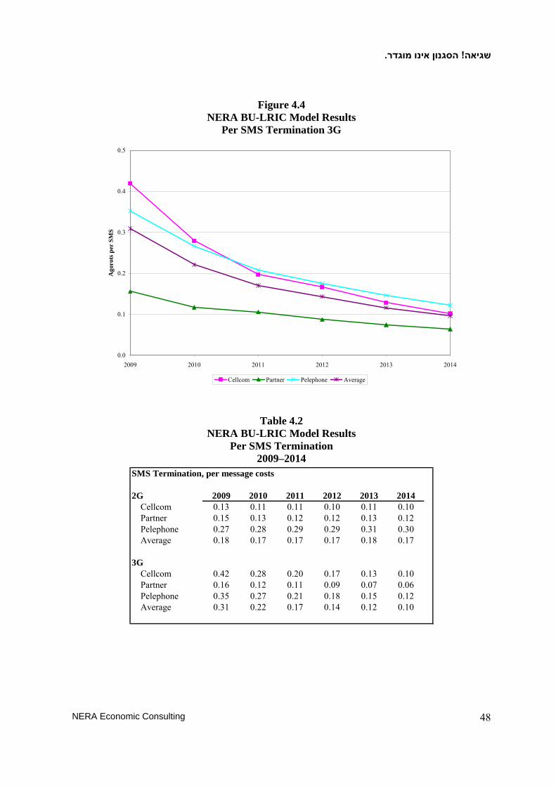
.הסגנון אינו מוגדר! שגיאה
NERA Economic Consulting 48
Figure 4.4 NERA BU-LRIC Model Results
Per SMS Termination 3G
0.0
0.1
0.2
0.3
0.4
0.5
2009 2010 2011 2012 2013 2014
Ago
rots
per
SM
S
Cellcom Partner Pelephone Average
Table 4.2
NERA BU-LRIC Model Results Per SMS Termination
2009–2014 SMS Termination, per message costs
2G 2009 2010 2011 2012 2013 2014Cellcom 0.13 0.11 0.11 0.10 0.11 0.10Partner 0.15 0.13 0.12 0.12 0.13 0.12Pelephone 0.27 0.28 0.29 0.29 0.31 0.30Average 0.18 0.17 0.17 0.17 0.18 0.17
3G 0.32 0.25 0.18 0.15 0.12 0.10Cellcom 0.42 0.28 0.20 0.17 0.13 0.10Partner 0.16 0.12 0.11 0.09 0.07 0.06Pelephone 0.35 0.27 0.21 0.18 0.15 0.12Average 0.31 0.22 0.17 0.14 0.12 0.10

.הסגנון אינו מוגדר! שגיאה
NERA Economic Consulting 49
4.3 MMS Termination
The LRIC estimates for MMS termination for Cellcom, Partner, and Pelephone are shown below.
Figure 4.5 NERA BU-LRIC Model Results
Per MMS Termination 2G
0.0
10.0
20.0
30.0
2009 2010 2011 2012 2013 2014
Ago
rots
per
MM
S
Cellcom Partner Pelephone Average
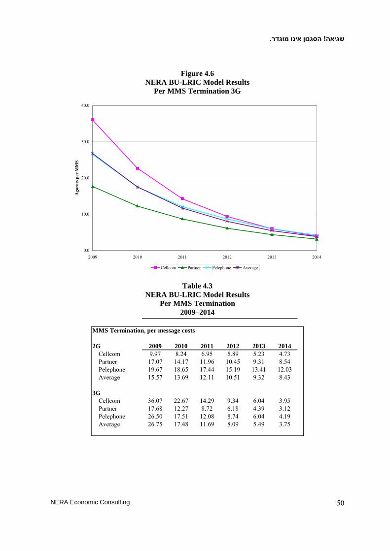
.הסגנון אינו מוגדר! שגיאה
NERA Economic Consulting 50
Figure 4.6 NERA BU-LRIC Model Results
Per MMS Termination 3G
0.0
10.0
20.0
30.0
40.0
2009 2010 2011 2012 2013 2014
Ago
rots
per
MM
S
Cellcom Partner Pelephone Average
Table 4.3 NERA BU-LRIC Model Results
Per MMS Termination 2009–2014
18.23 17.34 15.96 13.84 12.31 11.11MMS Termination, per message costs
2G 2009 2010 2011 2012 2013 2014Cellcom 9.97 8.24 6.95 5.89 5.23 4.73Partner 17.07 14.17 11.96 10.45 9.31 8.54Pelephone 19.67 18.65 17.44 15.19 13.41 12.03Average 15.57 13.69 12.11 10.51 9.32 8.43
3G 24.47 16.14 10.98 7.90 5.48 3.81Cellcom 36.07 22.67 14.29 9.34 6.04 3.95Partner 17.68 12.27 8.72 6.18 4.39 3.12Pelephone 26.50 17.51 12.08 8.74 6.04 4.19Average 26.75 17.48 11.69 8.09 5.49 3.75

.הסגנון אינו מוגדר! שגיאה
NERA Economic Consulting 51
4.4 Data Termination
The LRIC estimates for data termination for Cellcom, Partner, and Pelephone are shown below. The figure and table also shows the simple average cost of all three large incumbents.
Figure 4.7 NERA BU-LRIC Model Results Per MB Data Termination 2G
0.0
20.0
40.0
60.0
80.0
100.0
120.0
140.0
2009 2010 2011 2012 2013 2014
Ago
rots
per
dat
a M
byte
Cellcom Partner Pelephone Average
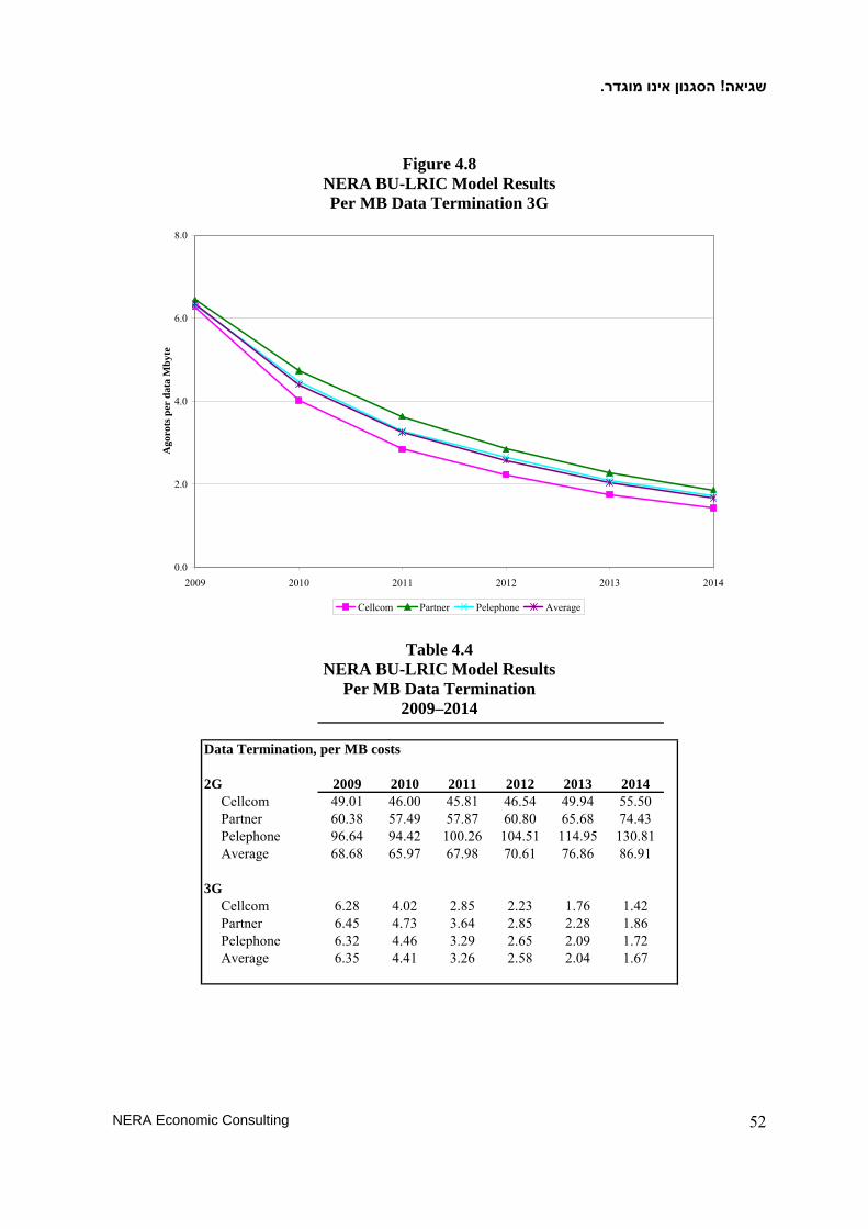
.הסגנון אינו מוגדר! שגיאה
NERA Economic Consulting 52
Figure 4.8 NERA BU-LRIC Model Results Per MB Data Termination 3G
0.0
2.0
4.0
6.0
8.0
2009 2010 2011 2012 2013 2014
Ago
rots
per
dat
a M
byte
Cellcom Partner Pelephone Average
Table 4.4 NERA BU-LRIC Model Results
Per MB Data Termination 2009–2014
89.96 88.16 95.72 101.82 114.27 132.33Data Termination, per MB costs
2G 2009 2010 2011 2012 2013 2014Cellcom 49.01 46.00 45.81 46.54 49.94 55.50Partner 60.38 57.49 57.87 60.80 65.68 74.43Pelephone 96.64 94.42 100.26 104.51 114.95 130.81Average 68.68 65.97 67.98 70.61 76.86 86.91
3G 5.89 4.14 3.00 2.43 1.94 1.61Cellcom 6.28 4.02 2.85 2.23 1.76 1.42Partner 6.45 4.73 3.64 2.85 2.28 1.86Pelephone 6.32 4.46 3.29 2.65 2.09 1.72Average 6.35 4.41 3.26 2.58 2.04 1.67

.הסגנון אינו מוגדר! שגיאה
NERA Economic Consulting 53
5 Policy Recommendation
We recommend that the MOC set MTRs for voice and SMS based on the average blended LRIC costs of the three existing mobile operators. The blended rate for an operator is the weighted average cost of its 2G and 3G LRIC, where the weights are the proportions of traffic run over its 2G and 3G networks. The blended rates for Cellcom, Partner, and Pelephone are then averaged, using a simple average. Using a simple average reflects the fact that neither MOC nor NERA has conducted an efficiency study. Hence, it cannot be readily determined that the carrier with the lowest costs (i.e., Cellcom in the case of 2009 voice LRIC) is the most efficient carrier since the operators use different technologies and/or have different frequency allocations. Similarly, it cannot be readily determined that the carrier with the highest costs (i.e., Pelephone in the case of 2009 voice LRIC) is the least efficient carrier. Rather, the differences in cost reflect the fact that each operator attempts to minimize its costs subject to different constraints, probably with different degrees of success. Hence, in order to minimize the average deviation from the (unobservable) most efficient set of costs, we recommend averaging the three carriers’ blended rates.
The specific policy recommendations, in real 2009 terms, for voice are derived and displayed in Table 5.1 and the specific recommendations for SMS are derived and displayed in Table 5.2.
Table 5.1 Voice (per minute) Policy Recommendation
Voice
Cellcom 2010 2011 2012 2013 20142G Cost 4.29 3.98 3.81 3.69 3.783G Cost 2.85 2.11 1.63 1.29 1.082G Weight 71% 67% 63% 58% 52%3G Weight 29% 33% 37% 42% 48%Blended Cost 3.88 3.37 3.00 2.67 2.48
Partner2G Cost 5.20 4.90 4.82 4.78 4.863G Cost 3.52 2.69 2.12 1.72 1.422G Weight 49% 46% 43% 39% 35%3G Weight 51% 54% 57% 61% 65%Blended Cost 4.33 3.71 3.28 2.92 2.63
Pelephone2G Cost 4.92 4.45 4.12 4.20 4.453G Cost 3.21 2.45 1.97 1.62 1.322G Weight 57% 54% 50% 46% 41%3G Weight 43% 46% 50% 54% 59%Blended Cost 4.19 3.53 3.05 2.81 2.61
Policy 4.14 3.54 3.11 2.80 2.57Recommendation

.הסגנון אינו מוגדר! שגיאה
NERA Economic Consulting 54
Table 5.2
SMS (per message) Policy Recommendation
SMS
Cellcom 2010 2011 2012 2013 20142G Cost 0.11 0.11 0.10 0.11 0.103G Cost 0.28 0.20 0.17 0.13 0.102G Weight 71% 67% 63% 58% 52%3G Weight 29% 33% 37% 42% 48%Blended Cost 0.16 0.14 0.13 0.12 0.10
Partner2G Cost 0.13 0.12 0.12 0.13 0.123G Cost 0.12 0.11 0.09 0.07 0.062G Weight 49% 46% 43% 39% 35%3G Weight 51% 54% 57% 61% 65%Blended Cost 0.12 0.11 0.10 0.10 0.08
Pelephone2G Cost 0.28 0.29 0.29 0.31 0.303G Cost 0.27 0.21 0.18 0.15 0.122G Weight 57% 54% 50% 46% 41%3G Weight 43% 46% 50% 54% 59%Blended Cost 0.27 0.25 0.24 0.22 0.20
Policy 0.19 0.17 0.16 0.14 0.13Recommendation
The policy recommendations are summarized in Table 5.3 below.
Table 5.3 Policy Recommendation Summary
2010 2011 2012 2013 2014
Voice (per minute) 4.14 3.54 3.11 2.80 2.57
SMS (per message) 0.19 0.17 0.16 0.14 0.13

Preliminary and Confidential Appendix A: Model Sensitivity Analyses
NERA Economic Consulting 55
Appendix A: Model Sensitivity Analyses Voice Termination, Blended 2G/3G LRIC costs 4.95 3.91 3.28 2.89 2.70 2.55
Unit cost (ILS agorot per voice min, SMS/MMS message or data Mbyte)Scenario Operator Depreciation Method Alternate Settings 2009 2010 2011 2012 2013 2014
1 Cellcom Tilted Straight Line 4.85 3.88 3.37 3.00 2.67 2.482 Cellcom Straight Line 4.43 3.54 3.08 2.75 2.46 2.293 Cellcom Sum of Digits 5.66 4.54 3.95 3.52 3.13 2.914 Cellcom Annuity 4.05 3.24 2.82 2.51 2.25 2.105 Cellcom Tilted Annuity 4.29 3.44 2.99 2.66 2.37 2.216 Cellcom Tilted Straight Line Special Coverage: TRUE 4.90 3.93 3.41 3.04 2.70 2.517 Cellcom Tilted Straight Line Use 10GBE: TRUE 4.86 3.89 3.38 3.01 2.68 2.498 Cellcom Tilted Straight Line Leased Line Discount: 10% 4.84 3.87 3.36 2.99 2.66 2.469 Cellcom Tilted Straight Line MNO-specific Backhaul, BTS: TRUE 5.01 4.00 3.46 3.07 2.73 2.53
10 Cellcom Tilted Straight Line MNO-specific Backhaul, Other: TRUE 6.10 5.06 4.49 4.01 3.56 3.3211 Cellcom Tilted Straight Line Pure LRIC 2.09 1.91 1.90 1.86 1.58 1.4812 Partner Tilted Straight Line 5.27 4.33 3.71 3.28 2.92 2.6313 Pelephone Tilted Straight Line 5.33 4.19 3.53 3.05 2.81 2.61
[Incumbent Average] Tilted Straight Line 5.15 4.14 3.54 3.11 2.80 2.57
SMS Termination, Blended 2G/3G LRIC costs 0.28 0.25 0.23 0.21 0.19 0.17
Unit cost (ILS agorot per voice min, SMS/MMS message or data Mbyte)Scenario Operator Depreciation Method Alternate Settings 2009 2010 2011 2012 2013 2014
1 Cellcom Tilted Straight Line 0.20 0.16 0.14 0.13 0.12 0.102 Cellcom Straight Line 0.17 0.14 0.12 0.11 0.10 0.093 Cellcom Sum of Digits 0.23 0.18 0.16 0.15 0.13 0.124 Cellcom Annuity 0.15 0.12 0.11 0.10 0.09 0.085 Cellcom Tilted Annuity 0.17 0.14 0.12 0.11 0.10 0.096 Cellcom Tilted Straight Line Special Coverage: TRUE 0.20 0.16 0.14 0.13 0.12 0.107 Cellcom Tilted Straight Line Use 10GBE: TRUE 0.20 0.16 0.14 0.13 0.12 0.108 Cellcom Tilted Straight Line Leased Line Discount: 10% 0.20 0.16 0.14 0.13 0.12 0.109 Cellcom Tilted Straight Line MNO-specific Backhaul, BTS: TRUE 0.19 0.16 0.13 0.13 0.12 0.1010 Cellcom Tilted Straight Line MNO-specific Backhaul, Other: TRUE 0.18 0.15 0.13 0.12 0.11 0.1011 Cellcom Tilted Straight Line Pure LRIC 0.03 0.01 0.01 0.03 0.03 0.0212 Partner Tilted Straight Line 0.15 0.12 0.11 0.10 0.10 0.0813 Pelephone Tilted Straight Line 0.30 0.27 0.25 0.24 0.22 0.20
[Incumbent Average] Tilted Straight Line 0.22 0.19 0.17 0.16 0.14 0.13
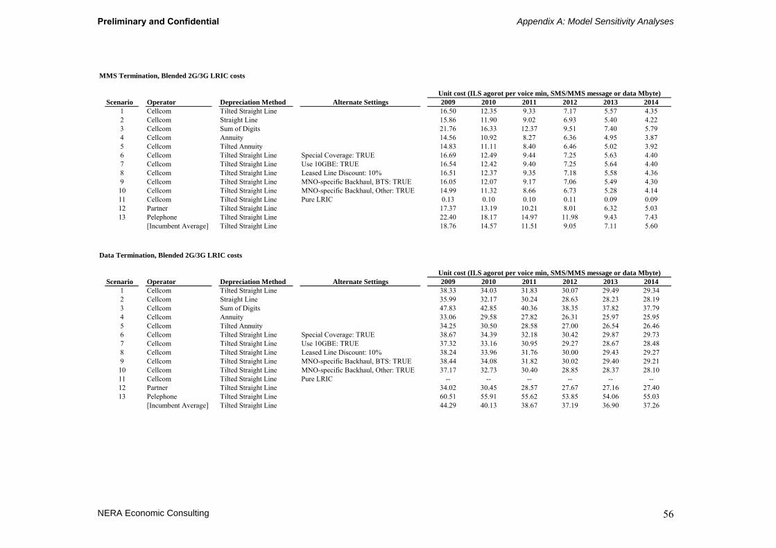
Preliminary and Confidential Appendix A: Model Sensitivity Analyses
NERA Economic Consulting 56
MMS Termination, Blended 2G/3G LRIC costs 20.73 16.82 13.67 10.88 8.63 6.82
Unit cost (ILS agorot per voice min, SMS/MMS message or data Mbyte)Scenario Operator Depreciation Method Alternate Settings 2009 2010 2011 2012 2013 2014
1 Cellcom Tilted Straight Line 16.50 12.35 9.33 7.17 5.57 4.352 Cellcom Straight Line 15.86 11.90 9.02 6.93 5.40 4.223 Cellcom Sum of Digits 21.76 16.33 12.37 9.51 7.40 5.794 Cellcom Annuity 14.56 10.92 8.27 6.36 4.95 3.875 Cellcom Tilted Annuity 14.83 11.11 8.40 6.46 5.02 3.926 Cellcom Tilted Straight Line Special Coverage: TRUE 16.69 12.49 9.44 7.25 5.63 4.407 Cellcom Tilted Straight Line Use 10GBE: TRUE 16.54 12.42 9.40 7.25 5.64 4.408 Cellcom Tilted Straight Line Leased Line Discount: 10% 16.51 12.37 9.35 7.18 5.58 4.369 Cellcom Tilted Straight Line MNO-specific Backhaul, BTS: TRUE 16.05 12.07 9.17 7.06 5.49 4.3010 Cellcom Tilted Straight Line MNO-specific Backhaul, Other: TRUE 14.99 11.32 8.66 6.73 5.28 4.1411 Cellcom Tilted Straight Line Pure LRIC 0.13 0.10 0.10 0.11 0.09 0.0912 Partner Tilted Straight Line 17.37 13.19 10.21 8.01 6.32 5.0313 Pelephone Tilted Straight Line 22.40 18.17 14.97 11.98 9.43 7.43
[Incumbent Average] Tilted Straight Line 18.76 14.57 11.51 9.05 7.11 5.60
Data Termination, Blended 2G/3G LRIC costs 56.33 52.19 53.04 52.39 53.67 55.59
Unit cost (ILS agorot per voice min, SMS/MMS message or data Mbyte)Scenario Operator Depreciation Method Alternate Settings 2009 2010 2011 2012 2013 2014
1 Cellcom Tilted Straight Line 38.33 34.03 31.83 30.07 29.49 29.342 Cellcom Straight Line 35.99 32.17 30.24 28.63 28.23 28.193 Cellcom Sum of Digits 47.83 42.85 40.36 38.35 37.82 37.794 Cellcom Annuity 33.06 29.58 27.82 26.31 25.97 25.955 Cellcom Tilted Annuity 34.25 30.50 28.58 27.00 26.54 26.466 Cellcom Tilted Straight Line Special Coverage: TRUE 38.67 34.39 32.18 30.42 29.87 29.737 Cellcom Tilted Straight Line Use 10GBE: TRUE 37.32 33.16 30.95 29.27 28.67 28.488 Cellcom Tilted Straight Line Leased Line Discount: 10% 38.24 33.96 31.76 30.00 29.43 29.279 Cellcom Tilted Straight Line MNO-specific Backhaul, BTS: TRUE 38.44 34.08 31.82 30.02 29.40 29.2110 Cellcom Tilted Straight Line MNO-specific Backhaul, Other: TRUE 37.17 32.73 30.40 28.85 28.37 28.1011 Cellcom Tilted Straight Line Pure LRIC -- -- -- -- -- --12 Partner Tilted Straight Line 34.02 30.45 28.57 27.67 27.16 27.4013 Pelephone Tilted Straight Line 60.51 55.91 55.62 53.85 54.06 55.03
[Incumbent Average] Tilted Straight Line 44.29 40.13 38.67 37.19 36.90 37.26

Preliminary and Confidential Appendix B: Demand Forecast Methodologies
NERA Economic Consulting 57
Appendix B: Demand Forecast Methodologies
Demand Variable Forecasting Method
Market SubscribersIsraeli population Forecasted using average 2004-2009 growth rate in populationMobile penetration (handset SIMs) Forecast using S-curve based on historical data from 1996 to 2009 - market close to saturation
Mobile subscribers (datacards) Forecast using average growth rate in datacard SIMs in Sweden between 2007 and 2009 and number of datacards in Israel in 2008. Datacards defined to include other devices like the recently launched ipad
Mobile penetration (handset SIMs + datacards) Calculated based on the number of handset SIMs (forecast above) plus forecast growth in data cards Percentage prepaid subscribers Forecasted using average 2004-08 growth rate (-0.9%)Percentage of GPRS subscribers Based on operator declaration of proportion of 2G subscribers that use GPRS
Percentage of 3G subscribers (handsets)Forecast based on proportion of 3G subscribers in 2008 in two early adopters of 3G technology (Japan & Korea. Forecasts in line with trends in 3G subscriber growth in Israel
Mobile subscribers (handset SIMs) Calculated: Israeli population * Mobile penetration (handset SIMs)Prepaid subscribers Calculated: Mobile handsets * % prepaidPostpaid subscribers Calculated: Mobile SIMs (handsets) * (1-%prepaid)GPRS subscribers Calculated: Mobile SIMs (handsets) * % GPRS3G handset subscribers Calculated: Mobile SIMs (handsets) * % 3G handsets2G subscribers Calculated: Mobile SIMs (handsets) - 3G handset subscribers
Market traffic volumes
Call volumes
Total M2M minutesTotal M2M minutes calculated based on M2M calling rate per subscriber forecasted using an S-curve based on 1996-2008 MOC data * Mobile SIMs (voice)
Mobile to mobile (on-net) – successful calls M2M on-net call minutes * (1/average successful on-net call duration based on operator data)
Mobile to mobile (on-net) – minutesTotal M2M minutes multiplied by average proportion of M2M calls that are on-net based on operator data
Mobile to mobile (off-net) – successful calls M2M off-net call minutes * (1/average successful off-net call duration based on operator data)Mobile to mobile (off-net) – minutes Total M2M minutes - M2M on-net minutes
Mobile to fixed – successful calls M2F call minutes * (1/average successful M2F call duration based on operator data)
Mobile to fixed – minutesTotal M2F minutes calculated based on M2F calling rate per subscriber forecasted using an S-curve based on 1996-2008 MOC data*Mobile SIMs (voice)
Mobile to international – successful calls M2Intl minutes* (1 /average successful M2Intl call duration based on operator data)Mobile to international – minutes Calculated as proportion of M2M + M2L calls that are M2Intl based on MOC data Fixed to mobile (termination) – successful calls F2M minutes * (1 / average F2M successful call duration based on operator data)
Fixed to mobile (termination) – minutesFixed subscribers forecast using constant 2004-2008 average growth rate*F2M calling rate per subscriber forecast using S-curve based on 1996-2008 data from MOC
Off-net mobile to mobile (termination) – successful calls M2M off-net termination minutes * (1 / average successful off-net to mobile termination call duration)
Off-net mobile to mobile (termination) – minutesCalculated based on average proportion of off-net mobile to mobile (termination) minutes to M2M off-net minutes
Other to mobile (termination) – successful calls Other to mobile minutes * (1 / average Intl2M call duration based on operator data)Other to mobile (termination) – minutes Calculated based on average proportion of Intl2M (termination) minutes to M2Intl minutes
Mobile to voicemail – successful callsCalculated based on average proportion of M2VM successful calls to sum of M2M on-net and off-net successful calls based on operator data
Mobile to voicemail – minutes M2VM successful calls * average M2VM call duration based on operator data
Fixed to voicemail – successful callsCalculated based on average proportion of F2VM successful calls to F2M successful calls based on operator data
Fixed to voicemail – minutes F2VM calls*average F2VM call duration based on operator data
This Appendix explains the various forecasting methods used to estimate the number of mobile subscribers and demand volumes which are used as inputs in the model. In general, we first forecast mobile subscribers and demand volumes for the Israeli market as a whole and then split these into operator level forecasts using operator market shares.

Preliminary and Confidential Appendix B: Demand Forecast Methodologies
NERA Economic Consulting 58
Demand Variable Forecasting MethodInternational roaming2G roaming on 2G- intl inbound roaming - successful calls Based on operator declarations for 2008-9 and assumed constant thereafter based on visitor trends2G roaming on 2G - intl inbound roaming - minutes Based on operator declarations for 2008-9 and assumed constant thereafter based on visitor trendsWCDMA roaming on 2G - successful calls Based on operator declarations for 2008-9 and assumed constant thereafter based on visitor trendsWCDMA roaming on 2G - minutes Based on operator declarations for 2008-9 and assumed constant thereafter based on visitor trends
SMS & MMS
Total outgoing SMS messagesMobile SIMs (handsets) * SMS messages per subscriberSMS messages per subscriber forecast based on average 2005-08 growth in SMS per subscriber in Israel
SMS messages on-net Calculated using average proportion of on-net SMS to total outgoing SMS based on operator data
SMS messages to other mobile networksCalculated using average proportion of SMS to other mobile to total outgoing SMS based on operator data
SMS messages to fixed networkCalculated using average proportion of SMS to fixed network to total outgoing SMS based on operator data
SMS messages from other networksCalculated using average proportion of SMS message from other networks to total outgoing SMS based on operator data
Total outgoing MMS messages Mobile SIMs (handsets) * MMS messages per subscriberMMS messages per subscriber forecast based on average 2005-08 growth in SMS per subscriber in Israel
MMS messages on-net Calculated using average proportion of on-net MMS to total outgoing MMS based on operator data
MMS messages to other mobile networksCalculated using average proportion of MMS to other mobile to total outgoing MMS based on operator data
MMS messages to fixed networkCalculated using average proportion of MMS to fixed network to total outgoing MMS based on operator data
MMS messages from other networksCalculated using average proportion of MMS message from other networks to total outgoing MMS based on operator data
Data
2G handset data volumeCalculated: 2G subscribers * forecast data usage per 2G subscriberData usage forecast using data provided by operators and data from UK, Portugal and Sweden
3G handset data volumeCalculated: 3G subscribers (handsets) * forecast data usage per 3G handsetData usage forecast using data provided by operators and data from UK, Portugal and Sweden
3G datacard data volumeCalculated: 3G subscribers (datacards) * forecast data usage per datacardData usage forecast using data provided by operators and data from UK, Portugal and Sweden
GPRS/EDGE service – on-net MS destinationCalculated: 2G handset data volume * GPRS/EDGE on-net MS destination data as a proportion of total 2G data from operator declarations
GPRS/EDGE service – on-net data centre destinationCalculated: 2G handset data volume * GPRS/EDGE on-net data centre destination data as a proportion of total 2G data from operator declarations
WCDMA data service – on-net MS destinationCalculated: 3G handset + datacard data volume * WCDMA on-net MS destination data as a proportion of total 3G data from operator declarations
WCDMA data service – on-net data centre destinationCalculated: 3G handset + datacard data volume * WCDMA on-net data centre destination data as a proportion of total 3G data from operator declarations
Proportion of traffic on 2G and 3GOn-net traffic % on 2GOn-net traffic % on 3GOutbound off-net traffic % on 2GOutbound off-net traffic % on 3GInbound off-net traffic % on 2GInbound off-net traffic % on 3GSMS on 2GSMS on 3G
Operator market sharesForecast using average 2007-2009 growth rate in operator market shares and increase in MIRS market share starting 2011
Operator subscribers and demand volumes For each operator, Operator market share x Market subscribers or market demand volumes
Based on 2G-3G traffic declarations made by operators and forecast assuming that the proportion of traffic carried over each operator's 2G network decreases with the forecast decrease in the proportion of 2G subscribers in the whole market.

Preliminary and Confidential Appendix B: Demand Forecast Methodologies
NERA Economic Consulting 59
Demand Variable Forecasting Method
Mobile to international – successful callsM2Intl minutes / average (M2Intl minutes per successful call) from operators
Mobile to international – minutes Sum of M2M min and M2L min *M2Intl per (M2M+M2L mins)Fixed to mobile (termination) – successful calls F2M minutes * average F2M successful call per minute
Fixed to mobile (termination) – minutes
Fixed subscriber 2008 (Telegeography), forecasted using constant 2007-2008 average growth rate*F2M min per sub, forecasted using an S-cuver based on 1996-2008 data from MOC.
Off-net mobile to mobile (termination) – successful callsM2M off-net minutes * average (off-net to mobile/M2M off-net) from operators
Off-net mobile to mobile (termination) – minutesOff-net to mobile minutes * average off-net mobile to mobile termination successful call per minute
Other to mobile (termination) – successful callsOther to mobile minutes / average (Intl2M min / successful calls) from operators
Other to mobile (termination) – minutes M2Intl minutes * average (Intl2M/M2Intl) from operators
Mobile to voicemail – successful calls(M2M on-net calls + M2M off-net calls)*average (VM2M calls/M2M calls) from operators
Mobile to voicemail – minutes M2VM calls * average (M2VM min/M2VM calls) from operatorsFixed to voicemail – successful calls L2M calls* average (L2VM calls / L2M calls) from operatorsFixed to voicemail – minutes L2VM calls*average (L2VM min/L2VM calls) from operatorsMobile data CSD – on-net MS destinationMobile data CSD – on-net data center destinationMobile data CSD – off-net (other mobile network) destinationMobile data CSD – fixed network destinationMobile data CSD – off-net incoming MS terminationMobile data CSD – off-net incoming data center termination2G roaming on 2GWCDMA roaming on 2G
SMS messages on-net
Mobile penetration * Israeli population* average SMS outgoing per sub from operators*moving four year average growth rate*average (on-net/total outgoing) from operators.
SMS messages to other mobile networksMobile penetration * Israeli population * average SMS outgoing per sub from operators*(off-net/total outgoing) from operators.
SMS messages to fixed networkMobile penetration * Israeli population * average SMS outgoing per sub from operators*(fixed/total outgoing) from operators.
SMS messages from other networksMobile penetration * Israeli population * average SMS outgoing per sub from operators*(incoming/total outgoing) from operators.
MMS messages on-net
Mobile penetration * Israeli population * average MMS outgoing per sub from operators**moving four year average growth rate*(incoming/total outgoing) from operators.
MMS messages to other mobile networksMobile penetration * Israeli population * average MMS outgoing per sub from operators*(off-net/total outoging) from operators
MMS messages to fixed networkMobile penetration * Israeli population * average MMS outgoing per sub from operators*(fixed/total outgoing) from operators.
MMS messages from other networksMobile penetration * Israeli population * average MMS outgoing per sub from operators*(incoming/total outgoing) from operators.
GPRS service – on-net MS destinationMobile penetration * Israeli population *(1- %3G)*data usage (MB) per sub (constant)*(GPRS/total 2G data) *(on-net MS/total GPRS)
GPRS service – on-net data center destinationMobile penetration * Israeli population *(1- %3G)*data usage (MB) per sub (constant)*(on-net data center/total GPRS)
GPRS service – off-net (other mobile network) destinationMobile penetration * Israeli population *(1- %3G)*data usage (MB) per sub (constant)*(GPRS/total 2G data) *(off-net destination/total GPRS)
GPRS service – fixed network destinationMobile penetration * Israeli population *(1- %3G)*data usage (MB) per sub (constant)*(GPRS/total 2G data) *(fixed network destination/total GPRS)
GPRS service – off-net incoming MS destinationMobile penetration * Israeli population *(1- %3G)*data usage (MB) per sub (constant)*(GPRS/total 2G data) *(incoming MS destination/total GPRS)
GPRS service – off-net incoming data center termination
Mobile penetration * Israeli population *(1- %3G)*data usage (MB) per sub (constant)*(GPRS/total 2G data) *(incoming data center termination/total GPRS)
EDGE data service – on-net MS destinationMobile penetration * Israeli population *(1- %3G)*data usage (MB) per sub (constant)*(EDGE/total 2G data)*(on-net MS/total GPRS)
EDGE data service – on-net data center destinationMobile penetration * Israeli population *(1- %3G)*data usage (MB) per sub (constant)*(EDGE/total 2G data)*(on-net data center/total GPRS)
EDGE data service – off-net (other mobile network) destinationMobile penetration * Israeli population *(1- %3G)*data usage (MB) per sub (constant)*(EDGE/total 2G data)*(off-net destination/total GPRS)
EDGE data service – fixed network destinationMobile penetration * Israeli population *(1- %3G)*data usage (MB) per sub (constant)*(EDGE/total 2G data)*(fixed network destination/total GPRS)
EDGE data service – off-net incoming MS destinationMobile penetration * Israeli population *(1- %3G)*data usage (MB) per sub (constant)*(EDGE/total 2G data)*(incoming MS destination/total GPRS)
EDGE data service – off-net incoming data center termination
Mobile penetration * Israeli population *(1- %3G)*data usage (MB) per sub (constant)*(EDGE/total 2G data)*(incoming data center termination/total GPRS)
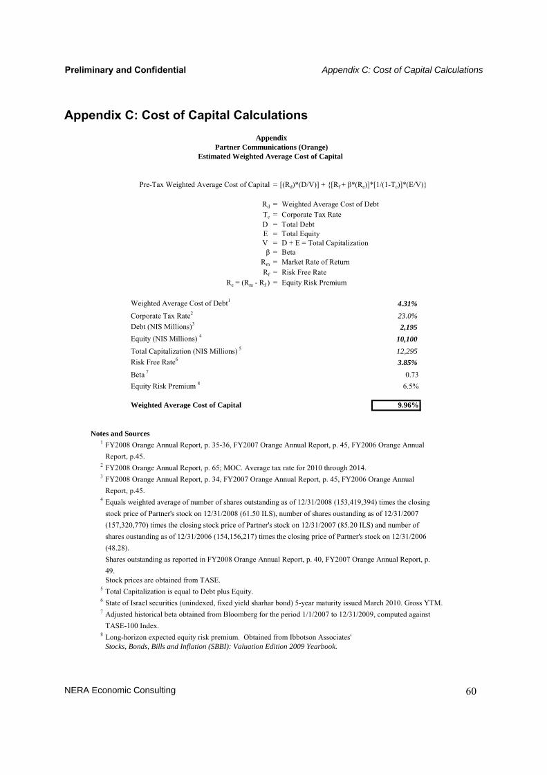
Preliminary and Confidential Appendix C: Cost of Capital Calculations
NERA Economic Consulting 60
Appendix C: Cost of Capital Calculations Appendix
Partner Communications (Orange)Estimated Weighted Average Cost of Capital
Pre-Tax Weighted Average Cost of Capital = [(Rd)*(D/V)] + {[Rf + β*(Re)]*[1/(1-Tc)]*(E/V)}
Rd = Weighted Average Cost of DebtTc = Corporate Tax RateD = Total DebtE = Total EquityV = D + E = Total Capitalizationβ = Beta
Rm = Market Rate of ReturnRf = Risk Free Rate
Re = (Rm - Rf ) = Equity Risk Premium
Weighted Average Cost of Debt1 4.31%Corporate Tax Rate2 23.0%Debt (NIS Millions)3 2,195Equity (NIS Millions) 4 10,100Total Capitalization (NIS Millions) 5 12,295Risk Free Rate6 3.85%Beta 7 0.73Equity Risk Premium 8 6.5%
Weighted Average Cost of Capital 9.96%
Notes and Sources1 FY2008 Orange Annual Report, p. 35-36, FY2007 Orange Annual Report, p. 45, FY2006 Orange Annual
Report, p.45.2 FY2008 Orange Annual Report, p. 65; MOC. Average tax rate for 2010 through 2014.3 FY2008 Orange Annual Report, p. 34, FY2007 Orange Annual Report, p. 45, FY2006 Orange Annual
Report, p.45.4 Equals weighted average of number of shares outstanding as of 12/31/2008 (153,419,394) times the closing
stock price of Partner's stock on 12/31/2008 (61.50 ILS), number of shares oustanding as of 12/31/2007(157,320,770) times the closing stock price of Partner's stock on 12/31/2007 (85.20 ILS) and number ofshares oustanding as of 12/31/2006 (154,156,217) times the closing price of Partner's stock on 12/31/2006(48.28).Shares outstanding as reported in FY2008 Orange Annual Report, p. 40, FY2007 Orange Annual Report, p.49.Stock prices are obtained from TASE.
5 Total Capitalization is equal to Debt plus Equity.6 State of Israel securities (unindexed, fixed yield sharhar bond) 5-year maturity issued March 2010. Gross YTM.7 Adjusted historical beta obtained from Bloomberg for the period 1/1/2007 to 12/31/2009, computed against
TASE-100 Index.8 Long-horizon expected equity risk premium. Obtained from Ibbotson Associates'
Stocks, Bonds, Bills and Inflation (SBBI): Valuation Edition 2009 Yearbook.
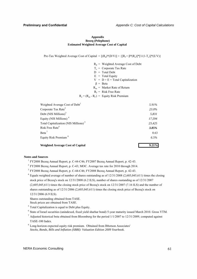
Preliminary and Confidential Appendix C: Cost of Capital Calculations
NERA Economic Consulting 61
AppendixBezeq (Pelephone)
Estimated Weighted Average Cost of Capital
Pre-Tax Weighted Average Cost of Capital = [(Rd)*(D/V)] + {[Rf + β*(Re)]*[1/(1-Tc)]*(E/V)}
Rd = Weighted Average Cost of DebtTc = Corporate Tax RateD = Total DebtE = Total EquityV = D + E = Total Capitalizationβ = Beta
Rm = Market Rate of ReturnRf = Risk Free Rate
Re = (Rm - Rf ) = Equity Risk Premium
Weighted Average Cost of Debt1 5.91%Corporate Tax Rate2 23.0%Debt (NIS Millions)3 5,831Equity (NIS Millions) 4 17,594Total Capitalization (NIS Millions) 5 23,425Risk Free Rate6 3.85%Beta 7 0.63Equity Risk Premium 8 6.5%
Weighted Average Cost of Capital 9.21%
Notes and Sources1 FY2008 Bezeq Annual Report, p. C-44-C46; FY2007 Bezeq Annual Report, p. 42-43.2 FY2008 Bezeq Annual Report, p. C-43; MOC. Average tax rate for 2010 through 2014.3 FY2008 Bezeq Annual Report, p. C-44-C46; FY2008 Bezeq Annual Report, p. 42-43.4 Equals weighted average of number of shares outstanding as of 12/31/2008 (2,605,045,611) times the closing
stock price of Bezeq's stock on 12/31/2008 (6.2 ILS), number of shares oustanding as of 12/31/2007(2,605,045,611) times the closing stock price of Bezeq's stock on 12/31/2007 (7.16 ILS) and the number ofshares outstanding as of 12/31/2006 (2,605,045,611) times the closing stock price of Bezeq's stock on12/31/2006 (6.9 ILS).Shares outstanding obtained from TASE.Stock prices are obtained from TASE.
5 Total Capitalization is equal to Debt plus Equity.6 State of Israel securities (unindexed, fixed yield sharhar bond) 5-year maturity issued March 2010. Gross YTM.7 Adjusted historical beta obtained from Bloomberg for the period 1/1/2007 to 12/31/2009, computed against
TASE-100 Index.8 Long-horizon expected equity risk premium. Obtained from Ibbotson Associates'
Stocks, Bonds, Bills and Inflation (SBBI): Valuation Edition 2009 Yearbook.

Preliminary and Confidential Appendix C: Cost of Capital Calculations
NERA Economic Consulting 62
AppendixCellcom
Estimated Weighted Average Cost of Capital
Pre-Tax Weighted Average Cost of Capital = [(Rd)*(D/V)] + {[Rf + β*(Re)]*[1/(1-Tc)]*(E/V)}
Rd = Weighted Average Cost of DebtTc = Corporate Tax RateD = Total DebtE = Total EquityV = D + E = Total Capitalizationβ = Beta
Rm = Market Rate of ReturnRf = Risk Free Rate
Re = (Rm - Rf ) = Equity Risk Premium
Weighted Average Cost of Debt1 5.12%Corporate Tax Rate2 23.0%Debt (NIS Millions)3 2,944Equity (NIS Millions) 4 10,228Total Capitalization (NIS Millions) 5 13,172Risk Free Rate6 3.85%Beta 7 0.66Equity Risk Premium 8 6.5%
Weighted Average Cost of Capital 9.37%
Notes and Sources1 FY2008 Cellcom Annual Report, p. F-24, FY2007 Cellcom Annual Report, p. 62, FY2006 Cellcom Annual
Report, p. 68.2 FY2008 Cellcom Annual Report, p. F-40; MOC. Average tax rate for 2010 through 2014.3 FY2008 Cellcom Annual Report, p. F-24, FY2007 Cellcom Annual Report, p. 62, FY2006 Cellcom Annual
Report, p. 68.4 Equals weighted average of number of shares outstanding as of 12/31/2008 (98,349,312) times the closing
stock price of Cellcom's stock on 12/31/2008 (85.25 ILS) and number of shares oustanding as of 12/31/2007(95,504,721) times the closing stock price of Cellcom's stock on 12/31/2007 (123.80 ILS).Shares outstanding as reported in FY2008 Cellcom 20-F, p. 2 and FY2007 Cellcom 20-F, p. 2.Stock prices are obtained from TASE.
5 Total Capitalization is equal to Debt plus Equity.6 State of Israel securities (unindexed, fixed yield sharhar bond) 5-year maturity issued March 2010. Gross YTM.7 Adjusted historical beta obtained from Bloomberg for the period 7/1/2007 to 12/31/2009, computed against
TASE-100 Index.8 Long-horizon expected equity risk premium. Obtained from Ibbotson Associates'
Stocks, Bonds, Bills and Inflation (SBBI): Valuation Edition 2009 Yearbook.

NERA Economic Consulting
NERA Economic Consulting 1 Front St., Suite 2600 San Francisco, California 94111 Tel: +1 415 291 1000 Fax: +1 415 291 1020 www.nera.com
NERA Economic Consulting 15 Stratford Place London W1C 1BE United Kingdom Tel: +44 20 7659 8500 Fax: +44 20 7659 8501 www.nera.com


