CHART SOLUTIONS FOR ANALYSIS OF EARTH SLOPES John H. Hunter, Department of Civil Engineering, Virginia Polytechnic Institute and

State University; and Robert L. Schuster, Department of Civil Engineering, University of Idaho

This paper compiles practical chart solutions for the slope stability prob­lem and is concerned with the use of the solutions rather than with their derivations. Authors introduced are Taylor, Bishop and Morgenstern, Morgenstern, Spencer, Hunter, and Hunter and Schuster. Many of the solu­tions introduced appeared originally in publications not commonly used by highway engineers. In addition to the working assumptions and param -eter definitions of each writer, the working charts are introduced, and example problems are included. The chart solutions cover a wide variety of conditions. They may be used to rapidly investigate preliminary de -signs and to obtain reasonable estimates of parameters for more detailed packaged computer solutions; in some cases, they may be used in the final design process.

•THE FIRST to make a valid slope stability analysis possible through use of simple charts and simple equations was Taylor (9 ). With the advent of high-speed electronic computers, other generalized solutions wilh different basic assumptions have been obtained and published. Unfortunately, these chart solutions have been published in several different sources, some of which are not commonly used by highway engineers in this country. This paper introduces several of these solutions that may prove useful and deals with how to use these solutions rather than with their derivations.

These chart solutions provide the engineer with a rapid means of determining the factor of safety during the early stages of a project when several alternative schemes are being investigated. In some cases they can be used in the final design procedure. Chart solutions such as these may very well serve as preliminary solutions for more detailed packaged computer software programs that are widely available (12).

Those chart solutions that appear to be most applicable to highway engineering prob­lems involving stability of embankment slopes and cut slopes are presented here. In addition to introducing some solutions that may be unfamiliar, this compilation pro­vides a quick means of locating various solutions so that rapid comparisons of advantages and disadvantages of each solution can be made.

The presentation of each solution includes pertinent references and contains sections on calculation techniques, working assumptions and definitions, limitations of the ap­proach, and an example problem. In each case only a sufficient number of curves have been shown to indicate the scope of the charts and to illustrate the solutions. The reader should refer to the appropriate references for greater detail.

TAYLOR SOLUTION

The solution found by Taylor (9, 10) is based on the friction circle (¢ cu·cle) method of analysis and his resulting charts are based on total stresses. Taylor made the fol­lowing assumptions for his solution:

1. A plane slope intersects horizontal planes at top and bottom. This is called a simple slope.

Sponsored by Committee on Embankments and Earth Slopes and presented at the 50th Annual Meeting . 77

78

2. The charts assume a circular trace for the failure surface.

3. The soil is an unlayered homoge­neous, isotropic material.

4. The shear strength follows Cou­lomb's Law so that s = c + ptan ¢.

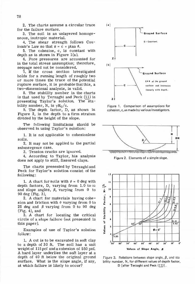
5. The cohesion, c, is constant with depth as is shown in Figure l(a).

6. Pore pressures are accounted for in the total stress assumption; therefore, seepage need not be considered.

7. If the cross section investigated holds for a running length of roughly two or more times the trace of the potential rupture surface, it is probable that this, a two-dimensional analysis, is valid.

8. The stability number in the charts is that used by Terzaghi and Peck (11) in presenting Taylor's solution. Thesta­bility number, N, is yHc/ c.

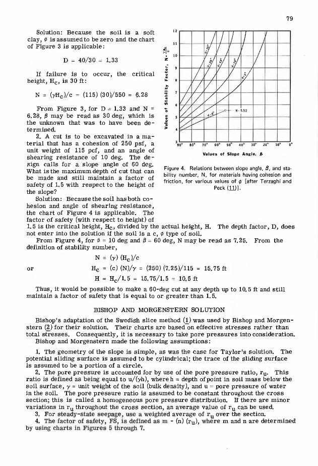
9. The depth factor, D, as shown in Figure 2, is the depth to a firm stratum divided by the height of the slope.

The following limitations should be observed in using Taylor's solution:

1. It is not applicable to cohesionless soils.

2. It may not be applied to the partial submergence case.

3. Tension cracks are ignored. 4. According to Taylor, his analysis

does not apply to stiff, fissured clays.

The charts presented by Terzaghi and Peck for Taylor's solution consist of the following:

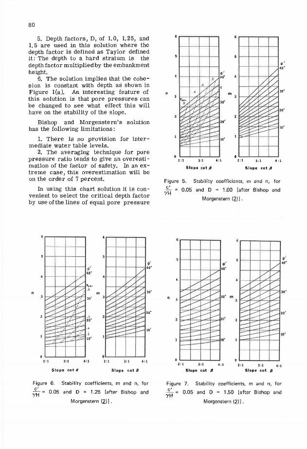
1. A chart for soils with ¢ = 0 deg with depth factors, D, varying from 1.0 to= and slope angles, {J, varying from 0 to 90 deg (Fig. 3 ),

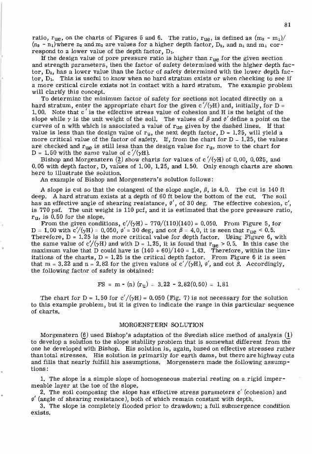
2. A chart for materials having cohe­sion and friction with ¢ varying from 0 to 25 deg and {J varying from 0 to 90 deg (Fig. 4), and

3. A chart for locating the critical cirde of a i:;lupe Iailu1·e (uul presenled in this paper).

Examples of use of Taylor's solution follow:

1. A cut is to be excavated in soft clay to a depth of 3 0 ft. The soil has a unit weight of 115 pcf and a cohesion of 550 psf. A hard layer underlies the soft layer at a depth of 40 ft below the original ground surface. What is the slope angle, if any, at which failure is likely to occur?

~Ju . z ~

!l u .. ... ~

:0 .: Ill -0

"' " .= .. >

(a)

Ground Surface

C::: Constant .

c

z

( b)

Ground Surface

C* 0 at the ground

c urfne ind lncrr-ou

linearly with depth .

z

Figure 1. Comparison of assumptions for cohesion, c, as made by various investigators.

~ ~ 7 tj· ~~~*~'*'"~~~

Figure 2. Elements of a simple slope.

12

11

10 I I I

~ wi! 0 .. • .,

!1 ii J J / ~ v VI

_.. _.. L,.../ O-m

60~ .....-n• 5.52

,,V v

rtJ~o" I

l . 85

390' 80' 70' 60' 50 40' JO ' 20 ' 10

Values of Slope Angle, 8

Figure 3. Relations between slope angla, f3, and sta­bility number, N, for different values of depth factor,

D [after Terzaghi and Peck (11)] .

Solution: Because the soil is a soft clay, ¢ is assumed to be zero and the chart of Figure 3 is applicable:

D = 40/30 = 1.33

If failure is to occur, the critical height, He, is 30 ft:

N = (yHc)/ c = (115) (30)/550 = 1,).28

~u " z .. ! u .. ... ; .a .. .. "' From Figure 3, for D = 1. 33 and N = 0

6. 28, {3 may be read as 3 0 deg, which is :: the unknown that was to have been de- .; termined. >

2. A cut is to be excavated in a ma -terial that has a cohesion of 250 psf, a

79

12

II

10

o•

Values of Slope Angle, /J, unit weight of 115 pcf, and an angle of shearing resistance of 10 deg. The de­sign calls for a slope angle of 60 deg. What is the maximum depth of cut that can be made and still maintain a factor of safety of 1. 5 with respect to the height of the slope?

Figure 4. Relations between slope angle, /3, and sta­bility number, N, for materials having cohesion and friction , for various values of ¢ [after Terzaghi and

Solution: Because the soil has both co­hesion and angle of shearing resistance, the chart of Figure 4 is applicable. The factor of safety (with respect to height) of

Peck (11)].

1. 5 is the critical height, He, divided by the actual height, H. The depth factor, D, does not enter into the solution if the soil is a c, </J type of soil.

From Figure 4, for ¢ = 10 deg and {3 = 60 deg, N may be read as 7.25. From the definition of stability number,

or

N = (y) (Hc)/c

He = (c) (N)/y = (250) (7.25)/115

H = Hc/l. 5 = 15. 75/1. 5 = 10. 5 ft

15. 75 ft

Thus, it would be possible to make a 60-deg cut at any depth up to 10. 5 ft and still maintain a factor of safety that is equal to or greater than 1. 5.

BISHOP AND MORGENSTERN SOLUTION

Bishop's adaptation of the Swedish slice method (1) was used by Bishop and Morgen­stern (2) for their solution, Their charts are based-on effective stresses rather than total stresses. Consequently, it is necessary to take pore pressures into consideration.

Bishop and Morgenstern made the following assumptions:

1. The geometry of the slope is simple, as was the case for Taylor's solution. The potential sliding surface is assumed to be cylindrical; the trace of the sliding surface is assumed to be a portion of a circle.

2. The pore pressure is accounted for by use of the pore pressure ratio, ru. This ratio is defined as being equal to u/(yh), where h = depth of point in soil mass below the soil surface, y = unit weight of the soil (bulk density), and u = pore pressure of water in the soil. The pore pressure ratio is assumed to be constant throughout the cross section; this is called a homogeneous pore pressure distribution. If there are minor variations in ru throughout the cross section, an average value of ru can be used.

3. For s teady-s tate seepage , use a weighted average of r u over the section. 4. The factor of safety, FS, is defined as m - (n) (ru), whe r e m and n are determined

by using charts in Figures 5 through 7.

80

5. Depth factors, D, of 1.0, 1.25, and 1. 5 are used in this solution where the depth factor is defined as Taylor defined it: The depth to a hard stratum is the depth factor multiplied by the embankment height.

6. The solution implies that the cohe­sion is constant with depth as shown in Figure l(a). An interesting feature of this solution is that pore pressures can be changed to see what effect this will have on the stability of the slope.

Bishop and Morgenstern's solution has the following limitations :

1. There is no provision for inter­mediate water table levels.

2. The averaging technique for pore pressure ratio tends to give an overesti­mation of the factor of safety. In an ex­treme case, this overestimation will be on the order of 7 percent.

In using this chart solution it is con­venient to select the critical depth factor by use of the lines of equal pore pressure

¢" 40"

n m 30°

30°

2 : 1 3:1 4 : 1 2 : 1 3 : 1 4 : 1

Slope cot 8 Slope cot /J

Figure 6. Stability coefficients, m and n, for c'

'YH = 0.05 and D = 1.25 [after Bishop and

Morgenstern (2.)] .

n m

o~-----2 :1 4: 1 2: 1 3: 1 4 : 1

Slope cot fl Slope cot fl

Figure 5. Stability coefficients, m and n, for c' 'YH = 0.05 and D = 1.00 [after Bishop and

Morgenstern (2)] .

¢ ' 40°

30°

m n 3

2: 1 3: 1 4 : 1 Slope cot fl Slope cot /J

Figure 7. Stability coefficients, m and n, for

c' 0.05 and D = 1.50 [after Bishop and 'YH

Morgenstern (2.)] .

81

ratio, rue, on the charts of Figures 5 and 6. The ratio, rue, is defined as (m2 - m 1 )/

(n2 - n1)where n2 and m2 are values for a higher depth factor, D2, and n1 and m 1 cor­respond to a lower value of the depth factor, D1.

If the design value of pore pressure ratio is higher than rue for the given section and strength parameters, then the factor of safety determined with the higher depth fac­tor, D2, has a lower value than the factor of safety determined with the lower depth fac­tor, D1. This is useful to know when no hard stratum exists or when checking to see if a more critical circle exists not in contact with a hard stratum. The example problem will clarify this concept.

To determine the minimum factor of safety for sections not located di rectly on a ha rd stratum, enter the appropriate chart for the given c

1/ (yH) and, initially , for D =

1. 00. Note that c' is the effective stress value of cohesion and H is the height of the slope while y is the unit weight of the soil. The values of f3 and </> ' define a point on the curves of n with which is associated a value of rue given by the dashed lines. If that value is less than the design value of ru, the next depth factor, D = 1. 2 5, will yield a more critical value of the factor of safety. If, from the chart for D = 1.25, the values are checked and rue is still less than the design value for ru, move to the chart for D = 1. 50 with the same value of c '/(yH).

Bishop and Morgenstern (2) show charts for values of c'/(yH) of 0.00, 0.025, and 0. 05 with depth factor, D, vaiUes of 1. 00, 1. 25, and 1. 50. Only enough charts are shown here to illustrate the solution.

An example of Bishop and Morgenstern's solution follows:

A slope is cut so that the cotangent of the slope angle, /3, is 4. 0. The cut is 140 ft deep. A hard stratum exists at a depth of 60 ft below the bottom of the cut. The soil has an effective angle of shearing resistance,¢', of 30 deg. The effective cohesion, c', is 770 psf. The unit weight is 110 pcf, and it is estimated that the pore pressure ratio, ru, is 0. 50 for the s lope.

From the given conditions , c'/(yH) = 770/(110)(140) = 0.050. From Figure 5, for D = 1. 00 with c'/(yH) = 0. 050, ¢' = 30 deg, and cot f3 = 4. 0, it is seen that rue < 0. 5. Therefore, D = 1.25 is the more critical value for depth factor. Using Figure 6, with the same value of c'/(yH) and with D = 1. 25, it is found that rue > 0. 5. In this case the maximum v.alue that D could have is (140 + 60)/140 = 1.43. Therefore, within the lim­itations of the charts, D = 1. 25 is the critical depth factor. From Figure 6 it is seen that m = 3. 22 and n = 2. 82 for the given values of c' / (yH ), ¢', and cot {3. Accordingly, the following factor of safety is obtained :

FS = m - (n) (ru) = 3.22 - 2.82(0.50) = 1.81

The chart for D = 1. 50 for c' / (yH) = 0. 050 (Fig. 7) is not necessary for the solution to this example problem, but it is given to indicate the range in this particular sequence of charts.

MORGENSTERN SOLUTION

Morgenstern (6) used Bishop's adaptation of the Swedish slice method of analysis (1) to develop a solution to the slope stability problem that is somewhat different from the one he developed with Bishop. His solution is, again, based on effective stresses rather than total stresses. His solution is primarily for earth dams, but there are highway cuts and fills that nearly fulfill his assumptions. Morgenstern made the following assump­tions:

1. The slope is a simple slope of homogeneous material resting on a rigid imper­meable layer at the toe of the slope.

2. The soil composing the slope has effective stress parameters c' (cohesion) and ¢'(angle of shearing resistance), both of which remain constant with depth.

3. The slope is completely flooded prior to drawdown; a full submergence condition exists.

82

4. The pore pressure ratio 7f, which is l::ii.u/ l::i,. ae11 is assumed to be unity during draw­down, and no dissipation of pore pressure occurs during drawdown.

5. The unit weight of the soil (bulk density), y, is assumed to be constant at twice the unit weight of water of 124. 8 pcf.

6. The pore pressure can be approximated by the product of the height of soil above a given point and the unit weight of water.

7. The drawdown ratio is defined as L/H where L is the amount of drawdown and H is the original height of the slope.

8. To be consistent, all assumed potential sliding circles must be tangent to the base of the section. This means that the value of H in the stability number, c'/(yH), and in L/H must be adjusted for intermediate levels of tangency (see the example problem for clarification).

Morgenstern's solution is particularly good for small dams·and consequently might be particularly applicable where a highway embankment is used as an earth dam or for flooding that might occur behind a highway fill. Another irnportant attribute of the method is that it permits partial drawdown conditions.

This method is somewhat limited by its strong orientation toward earth dams. If a core exists, it is noted that this violates the assumption of a homogeneous material. Another limitation is the assumption that the unit weight is fixed at 124. 0 pcf. Atten­tion is also called to the assumption of an impermeable base.

Morgenstern's charts cover a range of stability numbers, c'/(yH), from 0.0125 to 0. 050 and slopes of 2 :1 to 5 :1. The maximum value of ¢J

1 shown on his charts is 40 deg.

Following are some example problems using Morgenstern's method:

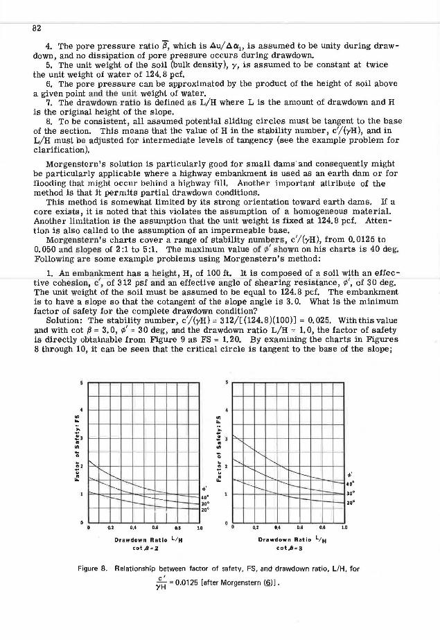
1. An embankment has a height, H, of 100 ft. It is composed of a soil with an effec­tive cohesi·on, c', of 312 psf and an effective angle of shearing resistance,¢', of 30 deg. The unit weight of the soil must be assumed to be equal to 124. 8 pcf. The embankment is to have a slope so that the cotangent of the slope angle is 3. 0. What is the minimum factor of safety for the complete drawdown condition?

Solution: The stability number, c'/(yH) = 312/[(124.8)(100)] = 0.025. With this value and with cot {3 = 3.0, ¢' = 30 deg, and the drawdown ratio L/H = 1.0, the factor of safety is directly obtainable from Figure 9 as FS = 1. 20. By examining the charts in Figures 8 through 10, it can be seen that the critical circle is tangent to the base of the slope;

"' ...

-0 .. 02 .. u :

f'-

" !'--..

"-f'--, -- :----.. I'-- r-_ r-- '--

-i-- r-- t--r--r---~ .._

I 0.2 0.4 0.6 0.8

Drawdown Ratio L;H

cot.8=2

r---,,,. 40° JO' 20•

1.0

"' ... ... .. : 3 .. "' -0 .. ! 2 u

:

"" r--....

0 0

""' .........

"" ...... ;-......, """ r--.._ 1--.. r--. '-

r-.. ......_ r--r--. t-. t--I--..___

r--~

0.2 0.4 0.6 0.8

Drawdown Ratio L;H

cot..B=3

--

¢'

40'

JO'

20•

1.0

Figure 8. Relationship between factor of safety, FS, and drawdown ratio, L/H, for c'

YH = 0.0125 [after Morgenstern (,6,)].

Ill ... .. ::­: , .. Ill -0 .. 0 z .. u if

"' ........_

-........_

......._

'- .......... ......

.......... r---- - :--_ ~i-- t--

o.z 0 .4 0 .6 0 .8

Draw down Rat Io L;H

cot ll - 2

~

<P' 40' 30' zo•

1.0

Ill ... ... ..

: 3 .. Ill -0

2 2 u .. ...

~

'" ....... ~ ""' i'--.. r---.... ,.._ ..... ......... -r--t--.._ t--

........ - - ...._ :----

0.2 0.4 0.6 0.8

Drawdown Ratio L;H cot 11~ 3

'--

-"'' 401

30'

zo•

1.0

Figure 9. Relationship between factor of safety, FS, and drawdown ratio, L/H, for c'

'YH = 0.025 [after Morgenstern 19.l] .

83

if any other tangency is assumed, H would have to be reduced. If His reduced, then the stability number is increased and this will, in all cases, result in a higher factor of safety.

2. It is now required to find the minimum factor of safety for a drawdown to mid­height of the section in the prior example.

Solution a: Considering slip circles tangential to the base of the slope, the effective height of the section, He, is equal to its actual height and the stability number remains

4 Ill ...

-0 .. ~z u

:.

"-r---..

"" I"--- ..._

0 0

['....:-...

I'-- !---... i'-..

r--~ .,;

----~ r-- _,__

40'

30'

zo• -- r-t-- ,..__

0.2- 0.4 o.& 0 .8

Drawdown Ratio L;H

cot ll= 2

~

1.0

Ill ... .. ... .. : 3 .. Ill -0

E 2 u .. ...

""' '- "!'--...

""" "-- i.......

'""' I""-.. r--.._ t---....

t---

'I'----- ........ r--"-- t--~

~1--~

o.z 0.4 0.6 0.1

Drawdown Ratio L;H

cot s ~ 3

.p' 40'

30'

zo•

1.0

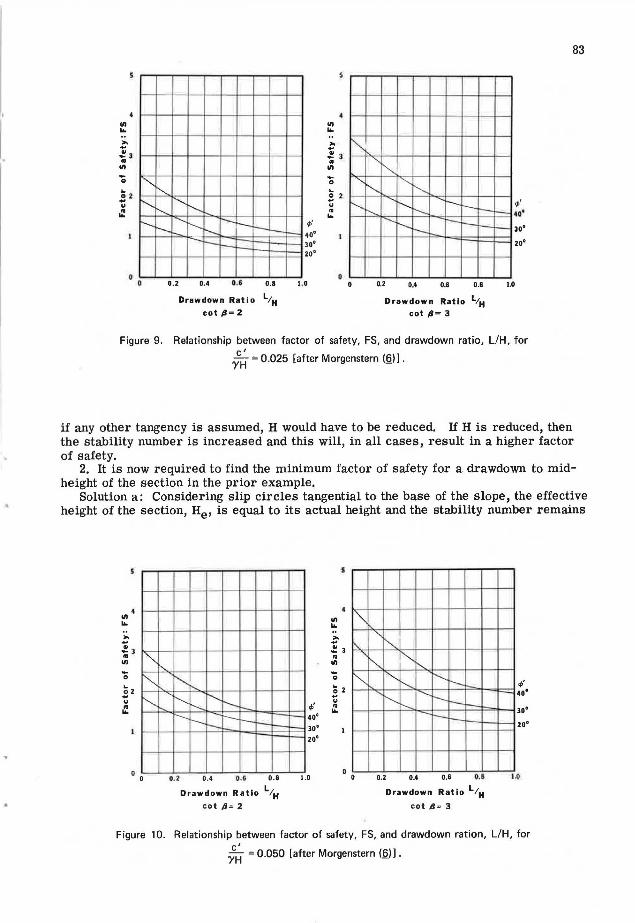
Figure 10. Relationship between factor of safety, FS, and drawdown ration, L/H, for c'

'YH = 0.050 [after Morgenstern (fil] .

unchanged as 0. 024. With this value of stability number and L/ He = 0. 50, and with other conditions remaining the same, the factor of safety may be read from Figure 9 as FS = 1. 52.

Solution b: Considering slip circles tangential to mid-height of the slope, the effec­tive height is equal to one-half the actual height so that He = H/ 2 = 100/ 2 = 50 ft. Thus c'/ (yHe) is twice that of the p revious solution or 0. 05, and L/ He = 1. 00. The minimum factor of safety, as determined by Morgenstern's solution, can be read directly from Figure 10 as FS = 1.48.

Solution c: Considering slip circles tangential to a level H/ 4 above the base of the slope, He becomes 3H/ 4 = 75 ft. Thus lhe slauilily number c'/(yHe) = 0.033, and L/He= 0. 67. The minimum factor of safety for this family must be obta ined by interpolation. From Figure 9 with c'/(yHe ) = 0.025, the factor of s afety is 1.31, and fro m Figure 10 with c'/(yHe) = 0. 05, the factor of safety is 1. 61. Interpolating linearly for c'/('YHe) = 0. 033, the minimum factor of safety for this family is 1. 31 + 0. 3 0/ 3 = 1.41.

These exampies demonstrate that for partial druwdown the critical circle may often lie above the base of the slope, and it is important to investigate several levels of tan­gency for the maximum drawdown level. In the case of complete drawdown, the mini­mum factor of safety is always associated with circles tangent to the base of the slope and the factor of safety at intermediate levels of drawdown need not be investigated. This may not be the case if the pore pressure distribution during drawdown differs sig­nificantly from that assumed by Morgenstern.

SPENCER SOLUTION

Bishop's adaptation of the Swedish slice method has been used by Spencer (8) to find a generalized solution to the slope stability problem. Spencer assumed paraliel inter­slice forces. His solution is based on effective stresses. Spencer defines the factor of safety, FS, as the quotient of shear strength available divided by the shear strength mobilized.

Spencer made the following additional assumptions and definitions for his solution:

1. The soils in the cut or embankment and underneath the slope are uniform and have similar properties.

2. The slope is simple and the potential slip surface is circular in profile. 3. A hard or firm stratum is at a great depth, or the depth factor, D, is very large. 4. The effects of tension cracks, if any, are ignored. 5. A homogeneous pore pressure distribution is assumed with the pore pressure

coefficient, ru, equal to u/{yh), where u = mean pore water pressure on base of slice, y = unit weight of the soil (bulk dens ity), and h = mean height of a slice.

6. The stability number N is defined as c'/[(FS)yHJ. 7. The mobilized angle of shearing resistance, ¢'m, is the angle whose tangent is

(tan ¢')/ FS.

Spencer's method does not prohibit the slip surface from extending below the toe. His solution permits the safe slope for an embankment of a given height to be found rapidly.

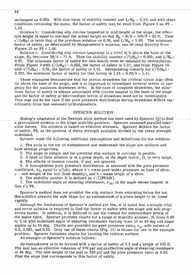
Although the limitations of Spencer's method are few, it is noted that a simple trial and error solution is required to find the factor of safety with the slope and soil prop­erties known. In addition, it is difficult to use his method for intermediate levels of the water table. Spencer provides charts for a range of stability number, N, from O. 00 to 0.12 with mobilized angle of shearing resistance varying from 10 to 40 deg and slope angles up to 34 deg. Charts are provided for pore pressure ratio , ru, with values of 0. 0, 0. 02 5, and O. 50. Only one of these charts {Fig. 11) is shown for use in the example problem. Spencer furnishes charts for locating the critical surface.

An example of Spencer's solution follows:

An embankment is to be formed with a factor of safety of 1. 5 and a height of 100 ft. The soil has an effective cohesion of 870 psf and an effective angle of shearing resistance of 26 deg. The unit weight of the soil is 120 pcf and the pore pressure ratio is 0. 50. Find the slope that corresponds to this factor of safety.

3: 1 2·: 1 15: 1

.10

-1"' u ~ .0

12 16 20 24 28 32

Slope : Decrees

Figure 11 . Relationship between stability number [- c-'- ] (FS) ?'H

and slope angle, 8, for various values of ¢fn [after Spencer {ft)].

Solution: The stability number,

N = c'/[ (FS}yH] 870/ [(1.5)(120)(100)] = 0.048

tan ¢.:n_ = (tan ¢')/FS = tan 26 deg/1. 5 = 0. 488/1. 5

tan ¢{n = 0.325 or ¢{n = 18 deg

85

Referring to Figure 11 for ru = 0. 50, the slope corresponding to a stability number of 0.48 and ¢{n = 18 deg is f3 = 18.4 deg. This corresponds approximately to a slope of 3 :1.

Linear interpolation between charts for slopes for ru values falling between the chart values is probably sufficiently accurate.

HUNTER SOLUTION

In 1968, Hunter (3) approached the slope stability problem with two assumptions that are different from the solutions previously presented in this paper. He assumed that the trace of the potential slip surface is a logarithmic spiral and the cohesion varies with depth. His charts are based on total stresses. Hunter's working assumptions and definitions follow:

1. The section of a cut is simple with constant slope, and top and bottom surfaces are horizontal.

2. The soil is saturated to the surface through capillarity. 3. The soil is normally consolidated, unfissured clay. 4. The problem is two-dimensional. 5. The shear strength can be described as s = c + p tan ¢ where c varies linearly with

depth, as is shown in Figure l(b ). It is assumed that the ratio c/p' is a constant, where p' is the effective vertical stress. Note that p' increases with depth.

6. If ¢ > 0 deg, the potential slip surface is a logarithmic spiral. If¢ = 0 deg, the potential failure surface is a circle because the logarithmic spiral degenerates into a circle for this case.

- ---- --------86

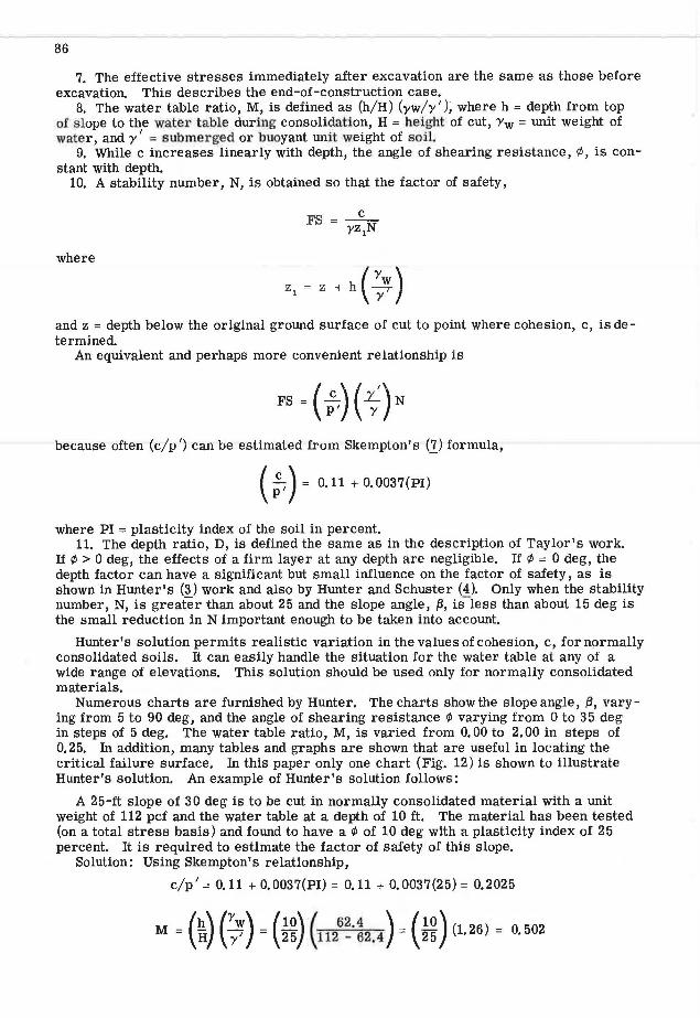
7. The effective stresses immediately after excavation are the same as those before excavation. This describes the end-of-construction case.

8. The water table ratio, M, is defined as (h/H) (yw/y' ); where h = depth from top of slope to the water table during consolidation, H = height of cut, 'Yw = unit weight of water, and y' = submerged or buoyant unit weight of soil.

9. While c increases linearly with depth, the angle of shearing resistance,¢, is con­stant with depth.

10. A stability number, N, is obtained so that the factor of safety,

where

and z = depth below the original ground surface of cut to point where cohesion, c, is de­termined

An equivalent and perhaps more convenient relationship is

because often (c/p') can be estimated from Skempton's (J_) formula,

(;,) = 0.11 +0.0037(PI)

where PI = plasticity index of the soil in percent. 11. The depth ratio, D, is defined the same as in the description of Taylor's work.

If ¢ > 0 deg, the effects of a firm layer at any depth are negligible. If ¢ = 0 deg, the depth factor can have a significant but small influence on the factor of safety, as is shown in Hunter's (3) work and also by Hunter and Schuster (4). Only when the stability number, N, is greater than about 25 and the slope angle, (3, is- less than about 15 deg is the small reduction in N important enough to be taken into account.

Hunter's solution permits realistic variation in the values of cohesion, c, for normally consolidated soils. It can easily handle the situation for the water table at any of a wide range of elevations. This solution should be used only for normally consolidated materials.

Numerous charts are furnished by Hunter. The charts show the slope angle, (3, vary­ing from 5 to 90 deg, and the angle of shearing resistance ¢ varying from 0 to 35 deg in steps of 5 deg. The water table ratio, M, is varied from O. 00 to 2. 00 in steps of 0.25. In addition, many tables and graphs are shown that are useful in locating the critical failure surface. In this paper only one chart (Fig. 12) is shown to illustrate Hunter's solution. An example of Hunter's solution follows:

A 25-ft slope of 30 deg is to be cut in normally consolidated material with a unit weight of 112 pcf and the water table at a depth of 10 ft. The material has been tested (on a total stress basis) and found to have a¢ of 10 deg with a plasticity index of 25 percent. It is required to estimate the factor of safety of this slope.

Solution: Using Skempton's relationship,

c/p' = 0.11+0.0037(PI) = 0.11 + 0.0037(25) = 0.2025

( h) ('Yw) (10) ( 62.4 ) (10) M = H ? = 25 112 - 62,4 = 25 (l. 26 ) = o. 5o2

,•

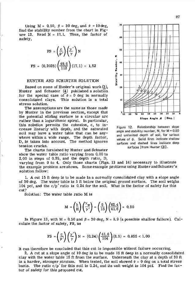
Using M = 0.50, f3 = 30 deg, and ¢ = lOdeg, find the stability number from the chart in Fig­ure 12. Read N = 17.1. Thus, the factor of safety,

FS = (0.2025) (i9i:) (17.1) = 1.52

HUNTER AND SCHUSTER SOLUTION

Based on some of Hunter's original work (3 ), Hunter and Schuster (4) published a solution for the special case oC ¢ = 0 deg in normally consolidated clays. This solution is a total stress solution.

The assumptions are the same as those made by Hunter in the previous section, except that the potential sliding surface is a circular arc rather than a logarithmic spiral. fu particular, this solution permits the cohesion, c, to in­crease linearly with depth, and the saturated soil may have a water table that can be any­where within a wide range. The depth factor, D, is taken into account. The method ignores tension cracks.

The charts furnished by Hunter and Schuster show the water table ratio varying from 0. 00 to 2.00 in steps of 0.25, and the depth ratio, D,

z . ~

10

60

50

.. 40 ... E

" z ... • ~ 30

... .. .. II)

20

10

i

~ .-

I

I I

:;1 I 1f.• v~ ~

~~ ~ "/

~ ~ f:::;::-~

J

7 I 7 J 77

7 i I } J 7 I

I/. [7 , 17 J ~ 1/

~ [)V'.. > v .

,...~ l/ c--- L.-- ..... i.--

0,0 80 70 60 50 40 JO 20 10

Slope Angle .JJ (Deg.)

87

I

Figure 12. Relationship between slope angle and stability number, N, for M = 050 and unlimited depth of soil, tor 11ario1.1s value~ of ¢ . Solid llnes indicate shallow surfaces and dashed lines indicate deep

surfaces [from Hunter(~)].

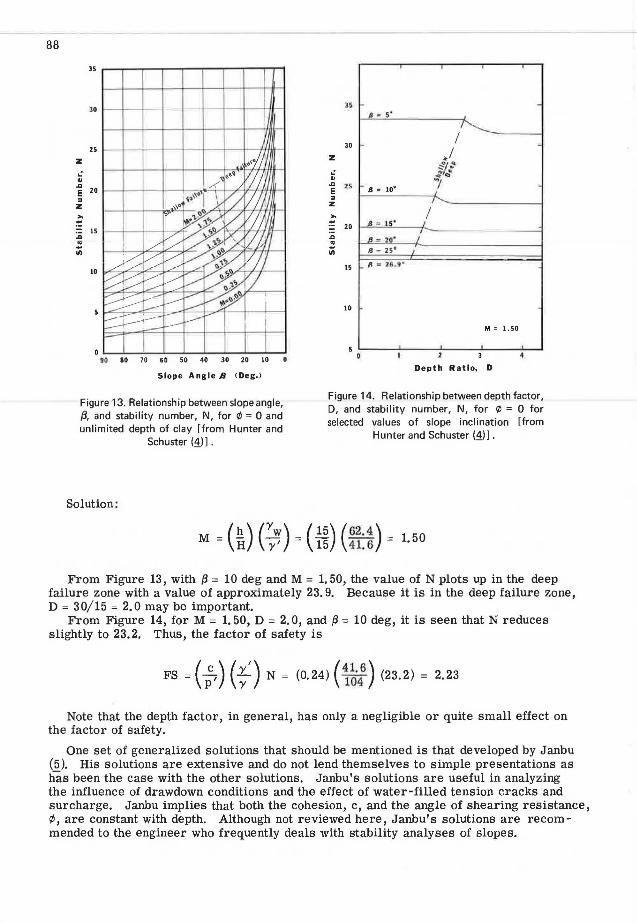
varying from 0 to 4. Only those charts (Figs. 13 and 14) necessary to illustrate the example problem are shown. Some example problems using Hunter and Schuster's solution follow:

1. A cut 15 ft deep is to be made in a normally consolidated clay with a slope angle of 30 deg. The water table is 5 ft below the original ground surface. The soil weighs 104 pcf, and the c/p / r atio is 0. 24 for the soil. What is the factor of safety for this cut?

Solution: The water table ratio Mis

M = (~) (:~) = ( ; 5) ( :;::) = 0.50

fu Figure 13, with M = 0.50 and f3 = 30 deg, N = 8. 9 (a possible shallow failure). Cal­culate the factor of safety, FS, ~s

FS = (.£..) (y') N = (0 24) (4

1.6

)(8 9) = 0.855 < 1.00 P' y • 104 .

It can therefore be concluded that this cut is impossible without failure occurring. 2. A cut at a slope angle of 10 deg is to be made 15 ft deep in a normally consolidated

clay with the water table 15 ft from the surface. Underneath the clay at a depth of 30 ft is a harder, stronger stratum. When tested, the soil showed ¢ = 0 deg on a total stress basis. The ratio c/p ' for this soil is 0.24, and its unit weight is 104 pcf. Find the fac­tor of safety for this proposed cut.

88

3S

J O

25

z .. ..

.Q

E 20

" z ... .. :a IS .. Vi

10

80 70 60 50 40 JO 20 10

Slope Angle IJ <Dec.>

Figure 13. Relationship between slope angle, {3, and stability number, N, for ¢ = 0 and unlimited depth of clay [from Hunter and

Schuster (1)] .

Solution:

'

35 - -11 • s· .

30

z

I ,_ ./

.:: .. .Q 2 S E

~ .. ' ~ .... ,_ II= 10•

7Q J

" z /'-

... I .. 20 .B: ,;a. 1-S' J

.Q

! fl)

s~ ••· I JJ = 25° J

IS ,. = 26 . 9"

10

M= I.SO

2

Depth Ratio, D

Figure 14. Relationship between depth factor, D, and stability number, N, for ¢ = 0 for selected values of slope inclination [from

Hunter and Schuster (1)] .

(h) (Yw) ( 15) (62.4) M = H ? = 15 41. 6 = 1. 5 0

From Figure 13, with f3 = 10 deg and M = 1. 50, the value of N plots up in the deep failure zone with a value of approximately 23. 9. Because it is in the deep failure zone, D = 30/ 15 = 2.0 may be important.

From Figure 14, for M = 1. 50, D = 2. O, and (3 = 10 deg, it is seen that N reduces slightly to 23.2. Thus, the factor of safety is

FS = (;,) (f) N = (0.24) ( i~46 ) (23.2) 2.23

Note that the depth factor, in general, has only a negligible or quite small effect on the factor of safety.

One set of generalized solutions that should be mentioned is that developed by Janbu (5). His solutions are extensive and do not lend themselves to simple presentations as has been the case with the other solutions. Janbu's solutions are useful in analyzing the influence of drawdown conditions and the effect of water-filled tension cracks and surcharge. Janbu implies that both the cohesion, c, and the angle of shearing resistance, ¢, are constant with depth. Although not reviewed here, Janbu's solutions are recom­mended to the engineer who frequently deals with stability analyses of slopes.

89

SUMMARY

The chart solutions developed by Taylor, Bishop and Morgenstern, Morgenstern, Spencer, Hunter, and Hunter and Schuster can be applied to a number of types of slope stability analyses. Some of the methods presented were originally developed only for cuts; some were developed especially for embankments or fills such as earth dams. Each solution presented, however, is applicable to some highway engineering situation. References have been given indicating more complex chart solutions not illustrated here, and an entry into the literature on computerized solutions has been given. Of the solutions introduced, those of Taylor, Hunter, and Hunter and Schuster are best suited to the short-term (end-of-construction) cases where pore pressures are not known and total stress parameters apply. The other methods are intended for use in long-term stability (steady seepage) cases with known effective stress parameters.

The methods make similar assumptions regarding slope geometry, two-dimensional failure, and the angle of shearing resistance being constant with depth. However, they vary considerably in assumptions regarding variation of cohesion, c, with depth, posi­tion of the water table, base conditions, drawdown conditions, and shape of the failure surface. Altogether, a wide range of conditions can be approximated by these available generalized solutions.

Each author has attempted to reduce the calculation time required to solve stability problems. The chart solutions alone may be sufficient for many highway problems; in other cases, chart solutions may save expensive computer time by providing a reason­able estimate as a starting point for computer programs that solve slope stability problems.

REFERENCES

1. Bishop, A. W. The Use of the Slip Circle in the Stability Analysis of Slopes. Geo­technique, Vol. 5, No. 1, 1955, pp. 7-17.

2. Bishop, A. W., and Morgenstern, N. Stability Coefficients for Earth Slopes. Geo­technique, Vol. 10, No. 4, 1960, pp. 129-150.

3. Hunter, J. H. Stability of Simple Cuts in Normally Consolidated Clays. PhD thesis, Dept. of Civil Engineering, Univ. of Colorado, Boulder, 1968.

4. Hunter, J. H., and Schuster, R. L. Stability of Simple Cuttings in Normally Consoli­dated Clays. Geotechnique, Vol. 18, No. 3, 1968, pp. 372-378.

5. Janbu, N. Stability Analysis of Slopes With Dimensionless Parameters. Harvard Soil Mechanics Series, No. 46, 1954, 81 pp.

6. Morgenstern, N. Stability Charts for Earth Slopes During Rapid Drawdown. Geo­technique, Vol. 13, No. 2, 1963, pp. 121-131.

7. Skempton, A. W. Discussion of "The Planning and Design of the New Hong Kong Airport." Proc. Institution of Civil Engineers, Vol. 7, 1957, pp. 305-307.

8. Spencer, E. A Method of Analysis of the Stability of Embankments Assuming Par­allel Inter-Slice Forces. Geotechnique, Vol. 17, No. 1, 1967, pp. 11-26.

9. Taylor, D. W. Stability of Earth Slopes. Jour. Boston Soc. of Civil Engineers, Vol. 24, 1937, pp. 197-246.

10. Taylor, D. W. Fundamentals of Soil Mechanics. John Wiley and Sons, Inc., New York, 1948, pp. 406-476.

11. Terzaghi, K., and Peck, R. B. Soil Mechanics in Engineering Practice. John Wiley and Sons, Inc., New York, 1967, pp. 232-254.

12. Whitman, R. V., and Bailey, W. A. Use of Computers for Slope Stability Analysis. Jour. Soil Mech. and Found. Div., ASCE, Vol. 93, No. SM4, Proc. Paper 5327, July 1967, pp. 475-498; also in ASCE "Stability and Performance of Slopes and Embankments," 1969, pp. 519-548.