188

Chemical Composition Measurements of
Cloud Condensation Nuclei and Ice Nuclei
by Aerosol Mass Spectrometry
Dissertation
zur Erlangung des Grades
�Doktor der Naturwissenschaften�
am Fachbereich Physik, Mathematik und
informatik
der Johannes Gutenberg-Universität
in Mainz
vorgelegt von
Paul Reitz
geboren in Ettelbruck, Luxemburg
Mainz, den 4. Juli 2011

b
Tag der Prüfung: 29. August 2011

Abstract
In this study the Aerodyne Aerosol Mass Spectrometer (AMS) was used during three
laboratory measurement campaigns, FROST1, FROST2 and ACI-03. The FROST
campaigns took place at the Leipzig Aerosol Cloud Interaction Simulator (LACIS)
at the IfT in Leipzig and the ACI-03 campaign was conducted at the AIDA facility
at the Karlsruhe Institute of Technology (KIT). In all three campaigns, the e�ect
of coatings on mineral dust ice nuclei (IN) was investigated.
During the FROST campaigns, Arizona Test Dust (ATD) particles of 200, 300
and 400 nm diameter were coated with thin coatings (<7 nm) of sulphuric acid. At
these very thin coatings, the AMS was operated close to its detection limits. Up
to now it was not possible to accurately determine AMS detection limits during
regular measurements. Therefore, the mathematical tools to analyse the detection
limits of the AMS have been improved in this work. It is now possible to calculate
detection limits of the AMS under operating conditions, without losing precious
time by sampling through a particle �lter.
The instrument was characterised in more detail to enable correct quanti�cation
of the sulphate loadings on the ATD particle surfaces. Correction factors for the
instrument inlet transmission, the collection e�ciency, and the relative ionisation
e�ciency have been determined. With these corrections it was possible to quantify
the sulphate mass per particle on the ATD after the condensation of sulphuric acid
on its surface.
The AMS results have been combined with the ice nucleus counter results. This
revealed that the IN-e�ciency of ATD is reduced when it is coated with sulphuric
acid. The reason for this reduction is a chemical reaction of sulphuric acid with the
particle's surface. These reactions are increasingly taking place when the aerosol
is humidi�ed or heated after the coating with sulphuric acid. A detailed analysis
of the solubility and the evaporation temperature of the surface reaction products
revealed that most likely Al2(SO4)3 is produced in these reactions.

Contents
Contents . . . . . . . . . . . . . . . . . . . . . . . . . . . . . . . . . . . . . . . . . . . . . . . . . . . . . . . . . . . iii
1 Introduction . . . . . . . . . . . . . . . . . . . . . . . . . . . . . . . . . . . . . . . . . . . . . . . . . . . . 1
1.1 Motivation . . . . . . . . . . . . . . . . . . . . . . . . . . . . . . . . . . . . . . . . . . . . . . . . . . . 1
1.2 Hygroscopic Growth, Droplets and Ice Formation . . . . . . . . . . . . . . . . . 3
1.2.1 Köhler Theory . . . . . . . . . . . . . . . . . . . . . . . . . . . . . . . . . . . . . . . . . . . 3
1.2.2 Ice Formation in the Atmosphere . . . . . . . . . . . . . . . . . . . . . . . . . . 5
1.3 Measurements under Extreme Instrumental Conditions . . . . . . . . . . . . . 7
2 Experimental Methods . . . . . . . . . . . . . . . . . . . . . . . . . . . . . . . . . . . . . . . . . 9
2.1 Aerosol Mass Spectrometer (AMS) . . . . . . . . . . . . . . . . . . . . . . . . . . . . . . 9
2.1.1 Instrument Description . . . . . . . . . . . . . . . . . . . . . . . . . . . . . . . . . . . 9
2.1.2 Modes of Operation . . . . . . . . . . . . . . . . . . . . . . . . . . . . . . . . . . . . . . 10
2.1.3 Electronic Baseline . . . . . . . . . . . . . . . . . . . . . . . . . . . . . . . . . . . . . . . 11
2.1.4 AMS Detection Limits . . . . . . . . . . . . . . . . . . . . . . . . . . . . . . . . . . . . 12
2.1.5 Mass to Charge Calibration . . . . . . . . . . . . . . . . . . . . . . . . . . . . . . . 13
2.1.6 Calculation of Aerosol Mass Concentration . . . . . . . . . . . . . . . . . . 14
2.1.7 Overshooting Duty Cycle Correction . . . . . . . . . . . . . . . . . . . . . . . 16
2.1.8 Tuning of the Ion Optics and Mass Spectrometer Electrodes . . . 17
2.1.9 Detection E�ciency Correction: Airbeam Correction . . . . . . . . . 17
2.1.10Data Evaluation . . . . . . . . . . . . . . . . . . . . . . . . . . . . . . . . . . . . . . . . . 18
2.2 Additional Instruments and Methods . . . . . . . . . . . . . . . . . . . . . . . . . . . . 18
2.2.1 Cloud Condensation Nuclei Measurements . . . . . . . . . . . . . . . . . . 18
2.2.2 Continuous Flow Di�usion Chamber . . . . . . . . . . . . . . . . . . . . . . . . 20
2.2.3 Leipzig Aerosol Cloud Interaction Simulator . . . . . . . . . . . . . . . . . 20
2.2.4 The Atmospheric Simulation Chamber AIDA . . . . . . . . . . . . . . . . 21
2.3 Arizona Test Dust . . . . . . . . . . . . . . . . . . . . . . . . . . . . . . . . . . . . . . . . . . . . 21
iv CONTENTS
2.4 BCR-66 Size Standards . . . . . . . . . . . . . . . . . . . . . . . . . . . . . . . . . . . . . . . . 22
2.5 Sulphuric Acid Coating Unit . . . . . . . . . . . . . . . . . . . . . . . . . . . . . . . . . . . 22
3 Continuous Determination of AMS Detection Limits . . . . . . . . . . . . 25
3.1 Classical Methods . . . . . . . . . . . . . . . . . . . . . . . . . . . . . . . . . . . . . . . . . . . . . 25
3.1.1 Counting Statistics . . . . . . . . . . . . . . . . . . . . . . . . . . . . . . . . . . . . . . . 25
3.1.2 Standard Deviation of Filter Measurements . . . . . . . . . . . . . . . . . 26
3.1.3 Frequency Space Closed Signal Analysis . . . . . . . . . . . . . . . . . . . . 26
3.1.4 Time Space Closed Signal Analysis . . . . . . . . . . . . . . . . . . . . . . . . . 29
3.2 Noise Retrieval in Time Space . . . . . . . . . . . . . . . . . . . . . . . . . . . . . . . . . . 29
3.2.1 Detrending of Closed Signals by Subtraction of a Running Mean 29
3.2.2 Detrending of Closed Signals Using Bezier Splines . . . . . . . . . . . . 31
3.2.3 Derivation of a Cubic Detrending Algorithm . . . . . . . . . . . . . . . . . 44
3.2.4 Computational complexity of the DL-cubic compared to the
Bezier method . . . . . . . . . . . . . . . . . . . . . . . . . . . . . . . . . . . . . . . . . . . 48
3.2.5 Test of the DL-cubic-Algorithm . . . . . . . . . . . . . . . . . . . . . . . . . . . . 49
3.2.6 Detection of Points Not Ful�lling the DL-cubic Prerequisites . . . 58
3.2.7 Application to Retrieve AMS Detection Limits . . . . . . . . . . . . . . . 60
3.2.8 Application and Limits of the Algorithm . . . . . . . . . . . . . . . . . . . . 61
3.3 Importance of the new continuous method . . . . . . . . . . . . . . . . . . . . . . . . 76
4 Improvements in Instrument Characterisation . . . . . . . . . . . . . . . . . . 79
4.1 Correction Factors . . . . . . . . . . . . . . . . . . . . . . . . . . . . . . . . . . . . . . . . . . . . 79
4.1.1 Transmission of the AMS Lens . . . . . . . . . . . . . . . . . . . . . . . . . . . . 80
4.1.2 Collection E�ciency of the AMS . . . . . . . . . . . . . . . . . . . . . . . . . . . 82
4.1.3 AMS Relative Ionisation E�ciency . . . . . . . . . . . . . . . . . . . . . . . . . 86
4.2 Signal Correction in the Case of Fast Decreasing AMS Closed Signal . 89
4.3 Summary of the Correction Factors . . . . . . . . . . . . . . . . . . . . . . . . . . . . . . 91
5 Laboratory Studies on the Ice Nucleation E�ciency of ATD . . . . 93
5.1 Experimental Set-up . . . . . . . . . . . . . . . . . . . . . . . . . . . . . . . . . . . . . . . . . . 93
5.2 Results and Discussion . . . . . . . . . . . . . . . . . . . . . . . . . . . . . . . . . . . . . . . . 97
5.2.1 Uncoated Dust Particles . . . . . . . . . . . . . . . . . . . . . . . . . . . . . . . . . . 97
5.2.2 Coating Mass per Particle . . . . . . . . . . . . . . . . . . . . . . . . . . . . . . . . . 100
5.2.3 Comparison of AMS Sulphate Concentrations to the
IN-E�ciency of ATD . . . . . . . . . . . . . . . . . . . . . . . . . . . . . . . . . . . . . 113
5.2.4 Sulphate Fragmentation Pattern: Evidence for ATD Surface
Etching . . . . . . . . . . . . . . . . . . . . . . . . . . . . . . . . . . . . . . . . . . . . . . . . . 117
CONTENTS v
5.2.5 Comparison of AMS Sulphate Concentrations to Soluble Mass
Concentrations . . . . . . . . . . . . . . . . . . . . . . . . . . . . . . . . . . . . . . . . . . 122
6 Aerosol Cloud Interaction Experiments at the AIDA . . . . . . . . . . . . 131
6.1 E�ect of Cloud Processing on Aerosol Composition . . . . . . . . . . . . . . . . 131
6.2 Detection of Coating on Mineral Dust During Cloud Activation
Experiments . . . . . . . . . . . . . . . . . . . . . . . . . . . . . . . . . . . . . . . . . . . . . . . . . 134
7 Conclusions and Outlook . . . . . . . . . . . . . . . . . . . . . . . . . . . . . . . . . . . . . . . 139
List of Figures . . . . . . . . . . . . . . . . . . . . . . . . . . . . . . . . . . . . . . . . . . . . . . . . . . . . . 143
List of Tables . . . . . . . . . . . . . . . . . . . . . . . . . . . . . . . . . . . . . . . . . . . . . . . . . . . . . . 153
List of Symbols and Abbreviations . . . . . . . . . . . . . . . . . . . . . . . . . . . . . . . . . 155
Publications Originating from this Thesis . . . . . . . . . . . . . . . . . . . . . . . . . . 163
References . . . . . . . . . . . . . . . . . . . . . . . . . . . . . . . . . . . . . . . . . . . . . . . . . . . . . . . . . 165


1
Introduction
1.1 Motivation
Clouds cover approximately 52 % of the sky over land and 65 % over ocean (Warren
et al., 1986) and (Warren et al., 1988), which corresponds to an average cloud cover-
age of 60 %. This cloud coverage in�uences the earth radiation budget by re�ecting
sunlight to space and trapping infrared radiation emitted by the earth (Seinfeld
and Pandis, 1998). Precipitating clouds transport water from the atmosphere to
the ground. However, 90 % of the clouds evaporate before precipitation occurs and
even when it occurs, some droplets evaporate prior to reaching the ground. Aerosol
particles interact with the clouds and in�uence their e�ect on the radiation budget
(Albrecht, 1989, DeMott et al., 2010, Lohmann and Feichter, 2005, Solomon et al.,
2007, Twomey, 1977). Furthermore chemical reactions in the aqueous phase take
place in cloud droplets, forming new compounds in the gas, the liquid and solid
phase (Seinfeld and Pandis, 1998, chapter 6).
Cloud drops do not form in particle free air but through condensation of water
on aerosol particles called cloud condensation nuclei (CCN). Whether a particle is
able to act as a CCN under the supersaturations found in the atmosphere depends
on its hygroscopicity and its size: larger particles and more hygroscopic particles act
more e�ciently as CCN. If more CCN are present in a cloud, more droplets form
and compete for the available water in the cloud. This results in an increase of the
droplet number concentration and a decrease of their size. In these clouds the light
from the sun is more e�ciently scattered back to space resulting in a higher cooling
e�ect. This is known as the �rst aerosol indirect e�ect (Twomey, 1977). A second
e�ect, referred to as the second aerosol indirect e�ect, is that by reducing the size
of the cloud droplets, it takes more time for the cloud to form drops which are big
enough to fall to the ground. High CCN concentrations thus result in a longer life
time of the clouds, enlarging the cloud coverage of the earth (Albrecht, 1989, Pincus
and Baker, 1994). In contrast under conditions with very low amounts of CCN, the
2 1 Introduction
amount of CCN can become a limiting factor for the formation of clouds, as was
reported by Mauritsen et al. (2011) for the Arctic.
Clouds can be composed of liquid water or ice or both phases. Below 0 ◦C,
the thermodynamicly stable phase of pure water is ice. However, water can be
supercooled down to approximately −38 ◦C without freezing, as an energy barrier
needs to be overcome for the formation of an ice crystal to start. Some solid surfaces,
so called ice nuclei (IN), show properties which lower the activation energy of the
freezing process. In the atmosphere these are often mineral dust particles as was
reported by Cziczo et al. (2004), DeMott et al. (2003), Kamphus et al. (2010), Mertes
et al. (2007) and Richardson et al. (2007) from the analysis of snow crystal residuals.
Additionally some authors state that biological particles like pollen (Diehl et al.,
2001, 2002, von Blohn et al., 2005), fungal spores and bacteria might be important
IN as some of them already induce freezing at temperature close to 0 ◦C (Möhler
et al., 2007, Morris et al., 2004, Szyrmer and Zawadzki, 1997). Christner et al. (2008)
state that biological IN are ubiquitous in snow but Hoose et al. (2010) found that
the concentration of biological IN is too low to be important on a global scale but
nevertheless they might be important on a local scale. Soot particles and metallic
particles were found to act as IN under cirrus cloud conditions (Chen et al., 1998,
DeMott et al., 1999). Cziczo et al. (2009) found that anthropogenic lead might
be an important constituent of IN. The exact properties responsible for a particle
incorporated in a droplet to act as an IN are still unknown for most systems.
The e�ect on the cloud albedo of aerosol particles acting as IN has been investi-
gated by DeMott et al. (2010), and Storelvmo et al. (2011) on a global scale using
models. Both state that the increase of IN in the atmosphere has a net warming ef-
fect, however Storelvmo et al. (2011) obtain a smaller e�ect, as their model includes
not only the cloud lifetime e�ect but also the cloud albedo e�ect of an increased IN
population. The albedo e�ect is similar to the one of CCN and increases the cloud
albedo when the IN concentration is higher. However, the life time e�ect is opposite
to the CCN e�ect, as the freezing of clouds promote the formation of precipitation
(Roedel, 2000). Lohmann and Diehl (2006) showed that not only the number con-
centration but also the chemical nature of IN is important for the e�ect on the earth
radiation budget.
In mid latitudes the formation of precipitation typically involves the ice phase
(Roedel, 2000). Cloud droplets start to sediment after their formation and evaporate
at the cloud base where the saturation ratio drops below 100 %. For precipitation
to form, the droplets must grow to a size which allows them to reach the ground
prior to their evaporation. In a liquid but supercooled cloud, a few droplets which

1.2 Hygroscopic Growth, Droplets and Ice Formation 3
incorporate IN freeze at temperatures well above −38 ◦C. The saturation vapour
pressure over ice is lower than over water due to the increased evaporation enthalpy
of ice compared to water. In the liquid cloud, the air is slightly supersaturated
with respect to water, which is a huge supersaturation with respect to ice. The
ice crystals can thus grow much faster than water droplets and form crytals with
su�cient settling velocities to reach the ground prior to evaporation within a few
minutes. While falling through the cloud, ice particles e�ciently scavenge additional
supercooled droplets on their way. If the ice melts before reaching the ground, it
rains, otherwise the ice reaches the ground as snow or hail (Pruppacher and Klett,
1997, chapter 13.3.1).
The preceding paragraphs show that ice nuclei play an important role in cloud
physics. Nevertheless, it was up to now not possible to determine the properties
of an IN responsible for its IN ability. In this thesis the nature of mineral dust
ice nuclei is analysed using Arizona Test Dust (ATD) as a model substance. In
the atmosphere mineral dust is often internally mixed with organic and inorganic
material due to particle ageing processes in the atmosphere (Falkovich et al., 2001,
Hinz et al., 2005, Sullivan and Prather, 2007, Sullivan et al., 2007, Wiacek and Peter,
2009). Such additions potentially in�uence the e�ciency of mineral dust particles
to act as ice nuclei (Gallavardin et al., 2008, Möhler et al., 2005, 2008, Niedermeier
et al., 2010, Sullivan et al., 2010a,b). In this thesis the e�ect of sulphuric acid on
the IN ability of ATD is studied. In Niedermeier et al. (2010) we showed that the
IN-ability of ATD is reduced by the sulphuric acid coating and in Sullivan et al.
(2010b) we demonstrated further that this loss is irreversible. The main goal of this
thesis was to determine why the sulphuric acid reduces the IN-ability of ATD, with
the objective to better understand the properties of the ATD that make it behave
as an IN.
1.2 Hygroscopic Growth, Droplets and Ice Formation
1.2.1 Köhler Theory
The interaction of aerosol particles with elevated relative humidities is described by
the Köhler theory. It links the water saturation vapour pressure over a �at water
surface (p◦) to saturation water vapour pressure (pw(Dp)) over a solution surface
with curvature radius Dp/2. This relation is expressed by the Köhler equation Eq.
(1.1) (Köhler, 1936, Seinfeld and Pandis, 1998).
lnpw(Dp)
p◦=
A
Dp
− B
D3p
(1.1)
4 1 Introduction
satu
ratio
n ra
tio
diameter / arbitrary unit
Scrit
Dcrit
Köhler curve Kelvin term Raoult term
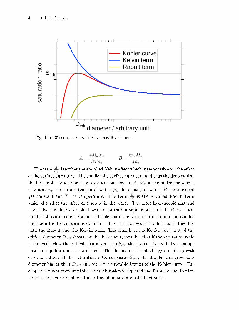
Fig. 1.1: Köhler equation with Kelvin and Raoult term.
A =4MwσwRTρw
B =6nsMw
πρw
The term ADp
describes the so-called Kelvin e�ect which is responsible for the e�ect
of the surface curvature. The smaller the surface curvature and thus the droplet size,
the higher the vapour pressure over this surface. In A, Mw is the molecular weight
of water, σw the surface tension of water, ρw the density of water, R the universal
gas constant and T the temperature. The term BD3
pis the so-called Raoult term
which describes the e�ect of a solute in the water. The more hygroscopic material
is dissolved in the water, the lower its saturation vapour pressure. In B, ns is the
number of solute moles. For small droplet radii the Raoult term is dominant and for
high radii the Kelvin term is dominant. Figure 1.1 shows the Köhler curve together
with the Raoult and the Kelvin term. The branch of the Köhler curve left of the
critical diameter Dcrit shows a stable behaviour, meaning that if the saturation ratio
is changed below the critical saturation ratio Scrit the droplet size will always adapt
until an equilibrium is established. This behaviour is called hygroscopic growth
or evaporation. If the saturation ratio surpasses Scrit, the droplet can grow to a
diameter higher than Dcrit and reach the unstable branch of the Köhler curve. The
droplet can now grow until the supersaturation is depleted and form a cloud droplet.
Droplets which grow above the critical diameter are called activated.

1.2 Hygroscopic Growth, Droplets and Ice Formation 5
Several modi�cations of the Köhler equation have been developed to take into
account di�erent e�ects like insoluble or partially soluble material as well as water
soluble gases in the surrounding air. In case of an insoluble core, as is the case for
an immersed mineral dust particle, the diameter in the Raoult term in Eq. (1.1) is
replaced by D3p − d3ic with d3ic being the e�ective diameter of the insoluble core.
Both forms of the Köhler equation described above are approximations of the real
physics for droplets with highly diluted solutes. If the solute is highly concentrated as
is the case for low saturation ratios, e.g. under smog conditions, the Köhler equation
can no longer be applied. Additional e�ects like e�orescence and deliquescence
become relevant (Seinfeld and Pandis, 1998). At low relative humidities salts are
dry and do not take up water. When the relative humidity is increased, the salts take
up water and are transformed to a highly concentrated solution at the deliquescence
relative humidity. If the relative humidity is again decreased, the salt recrystallises
at the e�orescence relative humidity, which is lower than the deliquescence relative
humidity. However, in this study, the measurements were conducted at humidities
close to and above water saturation and therefore the Köhler equation is a suitable
model.
1.2.2 Ice Formation in the Atmosphere
Homogeneous Freezing
Homogeneous freezing takes place at low temperatures in the absence of ice nuclei.
It is thought to be important for the formation of cirrus clouds (Heyms�eld and
Miloshevich, 1993, Jensen et al., 1998) and polar stratospheric clouds (Carslaw et al.,
1998, Jensen et al., 1991, Peter, 1997, Tabazadeh et al., 1997). However, more recent
publications also propose di�erent heterogeneous mechanism for the formation of
cirrus clouds (Abbatt et al., 2006, Murray et al., 2010). For the freezing of a water
droplet or solute to start in the absence of an heterogeneous ice nucleus a critical ice
embryo must form in the droplet. Simulations by Matsumoto et al. (2002) indicate
that this can happen when an ice like structure forms by statistical �uctuations
and at the same time the density of the droplet is slightly reduced due to local
density �uctuations. Temperatures below −35 ◦C are necessary for the formation of
a critical embryo to become likely in pure water. Solution droplets show even lower
temperatures for the onset of homogeneous ice nucleation.
Heterogeneous Freezing
Heterogeneous freezing can take place in four di�erent ways (Pruppacher and Klett,
1997, chapter 9.2). If the air is subsaturated with respect to water but supersatu-

6 1 Introduction
rated with respect to ice, water molecules can deposit on the ice nuclei and directly
form ice without the intermediate of the liquid phase. This process is called depo-
sition freezing. If the air is supersaturated with respect to water, water droplets
can form prior to freezing. If the droplets formed on the IN at temperatures above
0 ◦C and freeze when the temperature is lower, the freezing mode is called immer-
sion freezing. If the droplets formed on the IN at temperatures already below 0 ◦C
and the freezing occurs during the condensation, the freezing mode is referred to
as condensation freezing. If the droplets formed without including an IN and the
ice nucleus gets into contact to the droplets from the outside, contact freezing takes
place.
There are two main theories to explain heterogeneous freezing. The �rst one is a
stochastic approach assuming that the freezing is of statistic nature with the surface
of the IN reducing the energy barrier for the critical ice embryo to form and thus
increasing the probability of ice formation at higher temperatures. The freezing rate
jhet for the stochastic approach is given in Eq. (1.2) (Pruppacher and Klett, 1997,
chapter 9.2). The presented form is shown in Niedermeier et al. (2010):
jhet(T ) =kT
hexp
(−∆F (T )
kT
)× ns exp
(−∆Ghet(T )
kT
)(1.2)
T is the temperature, h the Planck and k the Boltzmann constant, and ns is
the number density of water molecules at the ice nucleus/water interface. ∆F (T )
describes the activation energy for crossing the liquid water/ice boundary. It rep-
resents a kinetic term for the growth of ice embryos. ∆Ghet(T ) is the Gibbs free
energy for the formation of a critical ice embryo in the presence of the respective
IN.
A second theory involves the hypothesis of ice active sites on the IN surface,
which trigger ice formation at a critical temperature as soon as this temperature is
reached. This theory was named singularity approach. The surface density na(T )
of ice active sites which are active at a temperature T is given by (Pruppacher and
Klett, 1997, chapter 9.2):
na(T ) = −∫ T
0◦C
k(θ)dθ (1.3)
where k(θ)dθ represents the number of sites per surface that become active in
the interval dθ.
The major di�erence between these two models is that in the stochastic approach,
the freezing can start at any temperature if the aerosol has enough time. The
presence of an IN is only increasing the probability that a particle freezes at higher

1.3 Measurements under Extreme Instrumental Conditions 7
temperatures and thus reduces the time necessary for the freezing. The singularity
approach assumes that the active sites on the particle surface trigger ice formation,
as soon as a certain temperature is reached. In Niedermeier et al. (2010), two models
have been derived from Eq. (1.2) and Eq. (1.3) to �t the number fraction of particles
that acted as IN in the immersion freezing mode at di�erent temperatures. Both
models �t the data well and thus no model could be discarded.
1.3 Measurements under Extreme Instrumental Conditions
The main instrument used in this thesis is the Aerodyne Aerosol Mass Spectrometer
(AMS) (Canagaratna et al., 2007, DeCarlo et al., 2006, Drewnick et al., 2005, Jayne
et al., 2000). It was used to chemically characterise sulphuric acid coatings on
Arizona Test Dust (ATD) which was used as model mineral dust ice nuclei. The ATD
itself cannot be evaporated in the AMS and therefore does not produce any signal.
Beside the disadvantage, that the AMS could not collect chemical information from
the ATD particles, the advantage was that small signals from coatings were not
disturbed by high signals from the particle core. After the characterisation, the AMS
was therefore suitable to chemically analyse coatings of a few nanometres, which are
relevant in the atmosphere, as well as their reactions with the ATD surface. These
reactions prooved to be the key reason for the reduction of the ATD IN e�ciency
when coated with sulphuric acid.
The particle size analysed in this thesis is in the range of a few 100 nm. This
size range is known as the accumulation mode. The particles in this mode have
the longest residence time in the atmosphere, which is typically around 10 days
(Pruppacher and Klett, 1997). Due to their long residence time, these particle are
omnipresent in the atmosphere and thus of highest importance for the interaction
with clouds.
Coatings of a few nm produce only low signals on the AMS detector. To avoid
interpreting data which is below the detection limit, it was necessary to develop a
method to determine detection limits under measurement conditions, which include
all factors involved. For this purpose an experimental method to determine AMS
detection limits as described by Drewnick et al. (2009) was improved to be appli-
cable under most experimental conditions. Furthermore, AMS measurements are
subject to several systematic errors linked to the collection e�ciency, the particle
size transmission range and more. In typical ambient experiments, these errors can
only be estimated or are completely inaccessible. However, under controlled labo-
ratory conditions, the instrument can be characterised to correct for these errors,
making quantitative measurements possible.
8 1 Introduction
Most of the data presented in this thesis was collected during the measurement
campaigns FROST1 and FROST2 (FReezing Of duST) at the institute for tropo-
spheric reasearch in Leipzig. The AMS sampled the ATD aerosol in parallel to the
Leipzig Aerosol Cloud Interaction Simulator (LACIS), to characterise the aerosol
which was introduced into LACIS. Further characterisation of the aerosol was per-
formed with additional instrumentation, whose data was combined with the AMS
data to complete the chemical charaterisation of the aerosol during the FROST
campaigns. The results of the FROST campaigns are presented in Chap. 5. In
addition to the FROST campaigns, the AMS participated at the ACI-03 (Aerosol
Cloud Interaction) campaign at the AIDA (Aerosol Interaction and Dynamics in
the Atmosphere) facility at the Karlsruhe Institute of Technology (KIT). These
measurements are dicussed in Chapt. 6.
2
Experimental Methods
2.1 Aerosol Mass Spectrometer (AMS)
2.1.1 Instrument Description
The Aerodyne Aerosol Mass Spectrometer (AMS) (Fig. 2.1) was �rst introduced by
Jayne et al. (2000) with a quadrupole detector (Q-AMS). The modi�cation of the
instrument used for this thesis was introduced by Drewnick et al. (2005). In this im-
proved version of the instrument the quadrupole mass spectrometer was exchanged
by a compact time of �ight mass spectrometer (C-TOF-AMS). A similar instrument
type was presented by DeCarlo et al. (2006), with a high resolution time of �ight
mass spectrometer (HR-TOF-AMS). The AMS measures mass spectra of aerosol
particles in the vacuum aerodynamic diameter (dva) range from 40 to 1000 nm, with
100 % inlet transmission e�ciency in the range of 60 to 600 nm. The vacuum aero-
dynamic diameter is the aerodynamic diameter of a particle in the free molecular
regime, meaning that the size of the particles is much smaller than the mean free
path of the air the particles are suspended in inside the instrument. It is an equiv-
alent diameter which corresponds to the diameter of a sphere of density 1 g/cm3
which experiences the same drag force in the the air as the probed particle. The
aerosol is introduced into the instrument via an aerodynamic lens which focuses the
aerosol particles on a thermal vaporiser, typically set to a temperature of 600 ◦C.
Particles which do not evaporate at the temperature the vaporiser is set to are ref-
ered to as refractory throughout this work. The vaporised particle compounds are
ionised by 70 eV electron impact and the resulting ions are introduced into a time
of �ight mass spectrometer via ion optics. After the time of �ight region, the ions
are detected by a multi channel plate (MCP) detector. As the air molecules are not
focused by the aerodynamic lens, the particles are enriched by a factor of 107 by
mass relative to gas molecules.

10 2 Experimental Methods
tof mass spectrometer
Aerosol vaporiser
Ionisation chamber
Turbo molecular pumps
ptof measurement
chopper Aerodynamic
inlet lens
MCP
Fig. 2.1: Schematics of the AMS modi�ed after Drewnick et al. (2005). ptof: particle timeof �ight, MCP: multi channel plate, preamp: preampli�er, ADC: analog digital converter.
2.1.2 Modes of Operation
The �rst mode of operation is the mass spectra mode (MS-mode). To separate the
particle signal from the background signal, the instrument is alternating between
the measurement of the background together with the particle signal (open) and
the measurement of the background alone with the particle beam blocked (closed).
In the open mode, the particle beam and the airbeam are measured by the instru-
ment. In the closed mode the aerosol is blocked and cannot reach the ioniser. The
closed signal is subtracted from the open signal, yielding mass spectra of the parti-
cles together with the remaining air ions which reached the vaporiser together with
the particle beam. The signal originating from the air can be separated from the
particle signal using a fragmentation table under the assumption that the ratios of
the concentrations of nitrogen, oxygen and argon are constant. The fragmentation
table is described in Allan et al. (2004). The factors in the fragmentation table are
determined by blank measurements using a particle �lter in front of the instrument.
A further important use of the fragmentation table is to attribute the signals of the
di�erent mass to charge ratios m/z to the corresponding chemical species, as di�er-
ent chemical substances often show signals on the same mass to charge ratios. The

2.1 Aerosol Mass Spectrometer (AMS) 11
main species distinguished by the AMS are nitrate, sulphate, ammonium, chloride
and organics. Molecules which are evaporated and ionised decompose into di�erent
fragments. Thus one molecule e.g. N2 produces signals on di�erent m/z. In the
case of N2 the main fragments are N+2 on m/z = 28 and N+ on m/z = 14. Addi-
tionally to the fragmentation, most molecules can include di�erent isotopes of their
composing elements. In case of N2 these are 14N and 15N resulting in additional
signals on m/z = 15, 29, 30. These signals interfere with other substances producing
signals on the same m/z e.g. C2H5+ on m/z = 29. As the ratios between di�erent
isotopes of most atoms in the atmosphere are known and rather stable, the strong
signals on m/z = 14 and m/z = 28 can be used to calculate the expected fractions
of m/z = 15, 29, 30 which belong to N2 and thus correct the intensities of other
substances which show a signal on these m/z. Similar to the isotopic ratios, the
fragmentation patterns for di�erent molecules are stable and can be corrected via
the table. Practically, the information used by the fragmentation table was gathered
in numerous laboratory studies (Allan et al., 2004) and as far as possible, the ratio
between di�erent fragments are determined for each instrument.
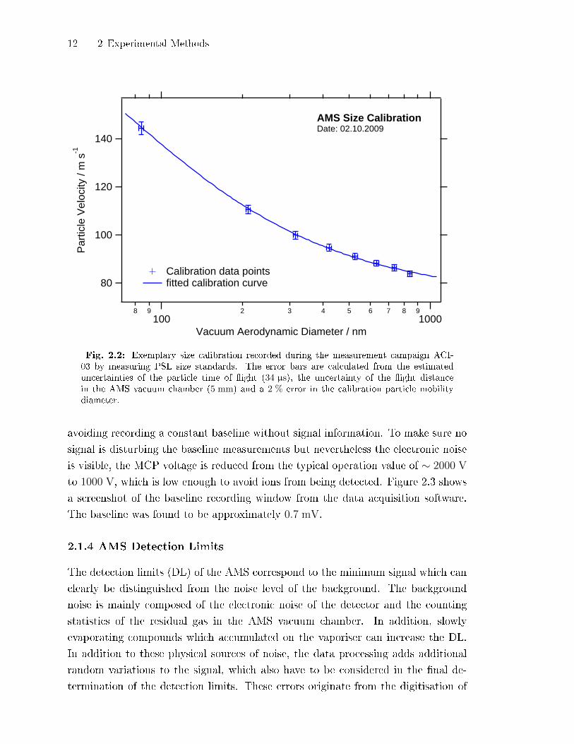
Beside the mass spectra, the AMS is able to determine the dva-distribution of
the aerosol particles. At the outlet nozzle of the aerodynamic lens the particles are
accelerated and reach di�erent terminal velocities depending on their dva. A chopper
with an opening time fraction of 2 % is used between the aerodynamic lens and the
vaporiser. During each cycle of the chopper, approximately 200 mass spectra are
recorded. The opening time of the chopper is recorded and thus the time when
particles can pass the chopper is known. The particles with lower dva have higher
velocities and arrive �rst at the ioniser and thus their mass spectra are recorded
�rst. The particle-time-of-�ight (PTOF) between the opening of the chopper and
the recording of the mass spectrum is converted into the dva using a calibration.
The calibration is performed using polystyrol latex size standards (PSL) and size
selected ammonium nitrate particles. An examplary size calibration curve is shown
in Fig. 2.2. As the size of the particles is determined by the particle time of �ight,
this mode is referred to as PTOF-mode.
2.1.3 Electronic Baseline
The signal of the AMS typically has an o�set which is blocking the lowest bits of
the anolog to digital conversion and reducing the dynamic range of the hardware.
To avoid this loss of dynamic range, the average voltage of the electronic noise, the
so called baseline, is determined and subtracted from the signal prior to recording.
The area below a signal is calculated for the signal above this systematic o�-set,
12 2 Experimental Methods
140
120
100
80
Par
ticle
Vel
ocity
/ m
s-1
8 9100
2 3 4 5 6 7 8 91000
Vacuum Aerodynamic Diameter / nm
AMS Size CalibrationDate: 02.10.2009
Calibration data points fitted calibration curve
Fig. 2.2: Exemplary size calibration recorded during the measurement campaign ACI-03 by measuring PSL size standards. The error bars are calculated from the estimateduncertainties of the particle time of �ight (34 µs), the uncertainty of the �ight distancein the AMS vacuum chamber (5 mm) and a 2 % error in the calibration particle mobilitydiameter.
avoiding recording a constant baseline without signal information. To make sure no
signal is disturbing the baseline measurements but nevertheless the electronic noise
is visible, the MCP voltage is reduced from the typical operation value of ∼ 2000 V
to 1000 V, which is low enough to avoid ions from being detected. Figure 2.3 shows
a screenshot of the baseline recording window from the data acquisition software.
The baseline was found to be approximately 0.7 mV.
2.1.4 AMS Detection Limits
The detection limits (DL) of the AMS correspond to the minimum signal which can
clearly be distinguished from the noise level of the background. The background
noise is mainly composed of the electronic noise of the detector and the counting
statistics of the residual gas in the AMS vacuum chamber. In addition, slowly
evaporating compounds which accumulated on the vaporiser can increase the DL.
In addition to these physical sources of noise, the data processing adds additional
random variations to the signal, which also have to be considered in the �nal de-
termination of the detection limits. These errors originate from the digitisation of

2.1 Aerosol Mass Spectrometer (AMS) 13
baseline
threshold
signal noise
sign
al/b
its
signal/m
V
time
Fig. 2.3: Screen shot of the AMS baseline determination window. The y-axis is inverted.The green line is the signal as recorded with the MCP at low voltage. The blue line is thebaseline and the red line is the baseline plus the threshold.
the analogue signal as well as from later o�-line corrections like the determination
of baselines.
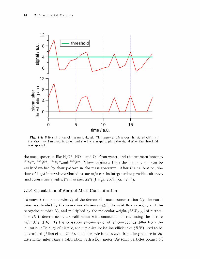
To reduce the AMS detection limit, the data is �ltered prior to the averaging
to reject signals which only contain noise. Data is only recorded if it is above a
threshold value, which is set in a way that it suppresses most of the noise but not
the smallest signals. In Fig. 2.4 the e�ect of thresholding is depicted on a generated
signal. Figure 2.3 shows the threshold set for the �rst week of the ACI-03 campaign
at the AIDA. Note that in the depicted signal no peak is above the threshold level.
To determine the highest level the threshold can be set to without loosing small
signals, the ratio of the ions resulting from nitrogen and argon is compared for
di�erent thresholds. In ambient air this ratio is constant. The signal from the
nitrogen is always clearly above the threshold, while argon often produces signals
composed of a single ion. If the value of the threshold becomes too high, the single
ion signals of the argon tend to be below the threshold, causing the ratio of argon
to nitrogen to drop. The threshold must not be set higher than the highest value
which does not yet cause small signals to be lost.
2.1.5 Mass to Charge Calibration
In the time of �ight mass spectrometer the ions are accelerated by a pulser elec-
trode. As all ions get approximately the same energy per charge, those ions with
the lowest mass to charge ratio (m/z) attain the highest velocity and arrive �rst at
the detector. The ion time of �ight is proportional to the square root of the m/z.
The proportionality factor is determined via the calibration with prominent m/z in
14 2 Experimental Methods
151050time / a.u.
12
8
4
0
sign
al /
a.u.
12
8
4
0sign
al a
fter
thre
shol
ding
/ a.
u. threshold
Fig. 2.4: E�ect of thresholding on a signal. The upper graph shows the signal with thethreshold level marked in green and the lower graph depicts the signal after the thresholdwas applied.
the mass spectrum like H2O+, HO+, and O+ from water, and the tungsten isotopes
182W+, 183W+, 184W+,and 186W+. These originate from the �lament and can be
easily identi�ed by their pattern in the mass spectrum. After the calibration, the
time-of-�ight intervals attributed to one m/z can be integrated to provide unit mass
resolution mass spectra (�sticks spectra�) (Hings, 2007, pp. 42-44).
2.1.6 Calculation of Aerosol Mass Concentration
To convert the count rates IS of the detector to mass concentration CS, the count
rates are divided by the ionisation e�ciency (IE ), the inlet �ow rate Qin and the
Avogadro number NA and multiplied by the molecular weight (MW NO3 ) of nitrate.
The IE is determined via a calibration with ammonium nitrate using the nitrate
m/z 30 and 46. As the ionisation e�ciencies of other compounds di�er from the
ionisation e�ciency of nitrate, their relative ionisation e�ciencies (RIE ) need to be
determined (Allan et al., 2003). The �ow rate is calculated from the pressure in the
instrument inlet using a calibration with a �ow meter. As some particles bounce o�

2.1 Aerosol Mass Spectrometer (AMS) 15
sign
al/b
its
time
Fig. 2.5: Screen shot of the AMS SI calibration window. The peak shown is the averagedsignal of 2380 single ion events.
the vaporiser before evaporation, the mass concentration needs to be divided by the
reduced collection e�ciency (CE ) due to this e�ect (Hu�man et al., 2005, Matthew
et al., 2008). The calculation of the mass concentration of a given species CS is
summarised in Eq. (2.1).
CS =1
RIES CES
· IS MWNO3
NA QinIENO3
(2.1)
The output voltage of the AMS detector after digitisation is in bits. The signal
of a certain m/z corresponds to the integrated signal in bits over the time bins
attributed to the m/z of interest. This yields a signal in bits · s which is converted
into ion counts by dividing it by the intensity of the signal of a single ion (SI). The
SI is recorded by measuring very low concentrations, as for example the residual gas
of the instrument without the typical air ions but with active thresholding in order
to avoid noise to be considered a small real signal. At mass to charge ratios with
very low signal, most of the signals originate from single ion events. These signals
are averaged to determine the single ion area. Figure 2.5 shows the averaged signal
of 2380 single ion peaks.
To calibrate the IE of the AMS, an ammonium nitrate solution is atomised and
the droplets are dried in two di�usion dryers. The dry particles are size selected in
a di�erential mobility analyser and the size selected particles are measured by the
AMS in the so called brute force single particle (BFSP) mode. In this mode the
signals of single particles is recorded by triggering the recording only when a certain
threshold is reached by the signal of the m/z the �lter is applied to. The chopper
16 2 Experimental Methods
MCP
pulser
refl
ecto
r
ion chamber
ion extractor ion lens1 ion lens2 deflector
deflector flange
filament
vaporiser
ion optics
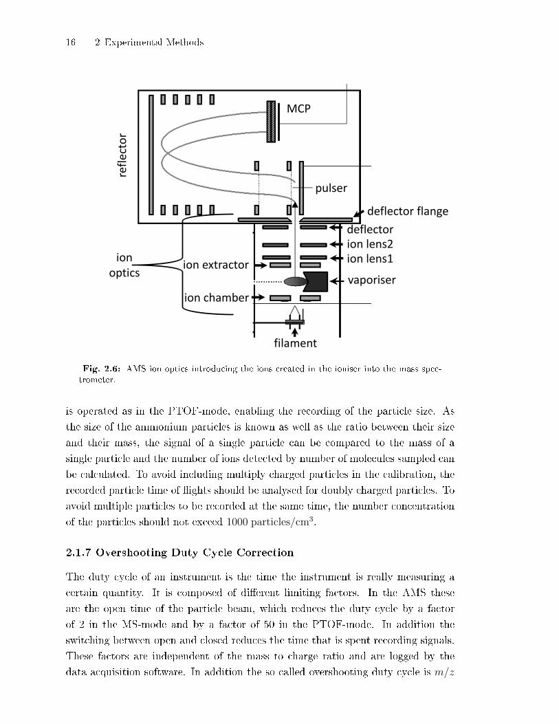
Fig. 2.6: AMS ion optics introducing the ions created in the ioniser into the mass spec-trometer.
is operated as in the PTOF-mode, enabling the recording of the particle size. As
the size of the ammonium particles is known as well as the ratio between their size
and their mass, the signal of a single particle can be compared to the mass of a
single particle and the number of ions detected by number of molecules sampled can
be calculated. To avoid including multiply charged particles in the calibration, the
recorded particle time of �ights should be analysed for doubly charged particles. To
avoid multiple particles to be recorded at the same time, the number concentration
of the particles should not exceed 1000 particles/cm3.
2.1.7 Overshooting Duty Cycle Correction
The duty cycle of an instrument is the time the instrument is really measuring a
certain quantity. It is composed of di�erent limiting factors. In the AMS these
are the open time of the particle beam, which reduces the duty cycle by a factor
of 2 in the MS-mode and by a factor of 50 in the PTOF-mode. In addition the
switching between open and closed reduces the time that is spent recording signals.
These factors are independent of the mass to charge ratio and are logged by the
data acquisition software. In addition the so called overshooting duty cycle is m/z
2.1 Aerosol Mass Spectrometer (AMS) 17
dependent. The ions are introduced into the mass spectrometer by the ion optics
which are shown in Fig. 2.6. The ions are accelerated into the mass spectrometer by
the voltage of the ion optics, mainly the voltage between the ion chamber and the ion
extractor. Depending on their m/z, the ions get di�erent velocities. After passing
the ion optics, the ions pass the pulser and are accelerated into the time of �ight
region. However, a fraction of the ions passes the pulser prior to the acceleration
pulse. These ions are lost for the �nal signal and thus the signal must be corrected
for this factor. The factor is proportional to the ion velocity and thereby to the
square root of the mass to charge ratio.
2.1.8 Tuning of the Ion Optics and Mass Spectrometer Electrodes
The voltages of the ion optics shown in Fig. 2.6, as well as those of the electrodes
inside the mass spectrometer need to be adjusted to obtain the optimal transmis-
sion and resolution of the instrument. Primary, maximum signal intensity must be
achieved. This is important, as only when the signal is maximised, the transmission
function of the ion optics introducing the ions into the mass spectrometer is inde-
pendent of the m/z of the ions. If the signal is not maximised, the ion transmission
becomes m/z dependent. Only after maximising the signal, the resolution can be
optimised (Trimborn, 2009). Because up to now their is no standardised way to de-
termine the ion transmission function, an m/z dependent ion transmission reduces
the quanti�cation ability of the AMS. The voltages of the mass spectrometer itself
can be tuned to get a good resolution without loosing �too much� signal. Adjusting
the voltage of the electrodes is achieved by scanning through the di�erent voltages,
starting with the ion optics. There is no standarised procedure to do this meaning
that the optimal tuning is achieved by trial and error.
2.1.9 Detection E�ciency Correction: Airbeam Correction
The detection e�ciency of the MCP detector of the AMS is decreasing with aging
time on scales of hours to days. To account for this e�ect, it is necessary to contin-
uously measure a constant quantity to monitor this loss in signal intensity. In the
AMS m/z 28, which corresponds to N+2 from the gas phase, is used for this purpose
as it always has a very high and constant signal which is only weakly in�uenced by
other ions. A reference value of the intensity of m/z 28 is recorded on calibration.
During the data evaluation process the ratio of the reference value and the measured
intensity on m/z 28 can be used to correct the measured mass concentrations for
the reduction of the e�ciency of the MCP. This e�ect is referred to as airbeam cor-
rection. When analysing closed or open data alone, the airbeam correction adds to
18 2 Experimental Methods
the noise of the signal. However, as the same factor is applied to both the closed and
the open signal, the noise introduced by the airbeam correction is mostly removed
when analysing the di�erence signal. This e�ect is important in Sect. 3.2.7 when
calculating AMS detection limits using the closed signal only.
2.1.10 Data Evaluation
The raw data of the AMS is typically evaluated using the software environment
Igor (WaveMetrics, Inc. Lake Oswego, Oregon, USA). The di�erent data evaluation
steps have been implemented as Igor procedures. These procedures, together with
a graphical user interface form the Igor software package SQUIRREL (http://cires.
colorado.edu/jimenez-group/ToFAMSResources/ToFSoftware/index.html). Nowa-
days SQUIRREL is used by basically the whole AMS community to perform the
standard data processing steps. This software also implements the fragmentation
table (see: Sect. 2.1.2) with default values, which can be adapted to the particular
experiments.
2.2 Additional Instruments and Methods
2.2.1 Cloud Condensation Nuclei Measurements
The cloud condensation nucleus properties of the aerosol during the FROST cam-
paigns were determined using a cloud condensation nucleus counter (CCNC) of the
type described in Roberts and Nenes (2005). The instrument was operated by Heike
Wex, IfT Leipzig. In this instrument, the supersaturation of the aerosol is scanned
in the range of 0.07 to 0.6 % at a controlled temperature. Those particles that acti-
vate as CCN grow to a size at which they can be counted optically. The number of
activated particles is then compared to the total number of aerosol particles yielding
the activated fraction at a given supersaturation.
Using single parameter Köhler theory (Petters and Kreidenweis, 2007, Wex et al.,
2007), the CCNC data can be translated into soluble mass per particle loadings if
the material of the soluble mass is known. Eq. (2.2) shows the single parameter
Köhler equation linking the size of the wet particle D to the saturation ratio S. Ddry
represents the dry diameter of the particle and A is a parameter depending on the
temperature and the surface tension at the solute/air interface.
S(D) =D3 −D3
dry
D3 −D3dry(1− κapp)
expA
D(2.2)
2.2 Additional Instruments and Methods 19
The parameter κapp is the apparent hygroscopicity parameter of the particle ma-
terial. It is composed of the sum of the apparent hygroscopicity parameters κi of
the di�erent compounds of the particle multiplied by their volume fraction εi (Eq.
(2.3)). The term �apparent� is used, as the hygroscopicity determined from the
CCNC measurements can be biased towards lower values if a fraction of the particle
material is only partially soluble. Material which is not soluble does not contribute
to the particle hygroscopicity and a�ects the CCN behaviour of the particles only
by increasing the particle dry diameter.
κapp =∑i
εiκi (2.3)
In case of a nearly insoluble particle core with a known soluble coating, Eq. (2.3)
simpli�es to Eq. (2.4) with the indices �coat� and �core� referring to the coating and
the particle core respectively.
κapp = εcoatκcoat + εcoreκcore (2.4)
The sum of the volume fractions must be equal to 1. If the apparent κ-value from
the particle core and the coating are known from preceding reference measurements
(Sullivan et al., 2009), Eq. (2.4) can be rearranged to determine the volume fraction
of the coating. The volume fraction is then multiplied by the total volume of the
particle (Vtotal) and multiplied by the density of the coating (ρcoat). This yields a
soluble coating mass per particle loading (msoluble), which can be compared to AMS
mass per particle loadings (Eq. (2.5)).
msoluble = ρcoat × Vcoat= ρcoat × Vtotal × εcoat= ρcoat × Vtotal ×
κapp − κcoreκcoat − κcore
(2.5)
The above technique works best if the particle core does not chemically react
with the coating on its surface. For the quartz particles coated with sulphuric acid,
which were used for reference experiments in these studies this was the case. If the
coating material reacts with the particle surface and the reaction products can not be
completely identi�ed and quanti�ed, the determination of the coating mass fraction
is restricted to an estimation assuming a probable surface material composition.
20 2 Experimental Methods
2.2.2 Continuous Flow Di�usion Chamber
The Continuous Flow Di�usion Chamber (CFDC) originally described by Rogers
et al. (2001) and modi�ed as described in Sullivan et al. (2010b), was operated
by Ryan Sullivan and Markus Petters (Colorado State University). It was used to
determine the number fraction of aerosol particles which nucleated ice at a set tem-
perature and water saturation ratio. The measurements and results were published
in Sullivan et al. (2010b). After cooling, the dry aerosol enters a region between
two concentric cylinders which are coated with ice. The cylinder walls are set to
di�erent temperatures in order to produce a supersaturated region with respect
to ice between the walls. The supersaturation is controlled via the temperatures
and can reach values above water saturation. If the aerosol is in a subsaturated
regime with respect to water, the freezing mechanism is deposition freezing (water
molecules deposit on the particle and form ice without passing the liquid phase). If
the aerosol gets supersaturated with respect to water, the freezing regime is either
immersion or condensation freezing (water passes the liquid phase prior to freez-
ing). The di�erent freezing mechanisms are described in (Pruppacher and Klett,
1997, chapter 9.2). The ice crystals are detected at the end of the chamber with an
optical particle counter. In order to prevent droplets from being detected together
with ice, a water subsaturated but ice saturated region follows the activation region.
In this region, the water droplets evaporate due to the Bergeron-Findeisen process
(Findeisen, 1938).
2.2.3 Leipzig Aerosol Cloud Interaction Simulator
The Leipzig Aerosol Cloud Interaction Simulator (LACIS) is a continuous �ow tube
which can be used to study both CCN and IN abilities of aerosols. However, in this
work only the IN-measurements of LACIS are used. It was operated by scientists
of the IfT in Leipzig and results have been published in Hartmann et al. (2011),
Niedermeier et al. (2010, 2011). The facility was introduced by Stratmann et al.
(2004) and its use for IN-studies is described in Hartmann et al. (2011). It consists
of a tube of seven metre length whose wall segments are temperature controlled.
The humidity of the aerosol is set to a controlled value at the beginning of the tube.
While passing the tube, the aerosol beam is surrounded by sheath air. Through the
lowering of the wall temperature, the aerosol is cooled down and thus its relative
humidity increases until particles activate as cloud droplets. By further lowering
the temperature, particles including an IN can freeze. At the outlet of the tube,
the particle size distribution is measured with an optical particle counter, which can

2.3 Arizona Test Dust 21
200 nm
Fig. 2.7: TEM picture of two ATD particles. Note the di�erence in the aspect ratiobetween the two particles indicated by the red circle and the blue oval. (TEM picture byA. Kiselev, Institute for Tropospheric Research, Leipzig and I. Lieberwirth, MPI-P, Mainz)
detect droplets and ice crystals. The retrieval of the ice and the droplet fraction
from the size distributions is described in Niedermeier et al. (2010).
2.2.4 The Atmospheric Simulation Chamber AIDA
The atmospheric simulation chamber AIDA (Aerosol Interaction and Dynamics in
the Atmosphere) (Möhler et al., 2001, Nink et al., 2000) at the Karlsruhe Institute
of Technology (KIT) consists of a vessel with a size of 84 m3. To simulate ascending
air parcels, so called expansion experiments can be performed in the chamber. The
chamber pressure is quickly reduced via pumping which provokes adiabatic cooling
of the air parcel. As in real atmospheric air parcels at a certain temperature the
water vapour pressure reaches supersaturation over ice and/or water. This way
cloud processing of aerosols and aerosol cloud interactions can be simulated. The
facility can be equipped with various instruments to characterise the air and the
particles in the chamber.
2.3 Arizona Test Dust
Arizona Test Dust is a mineral dust which is industrially produced from natural
sand collected in the desert of Arizona by Powder Technology Inc. (Burnsville, MN
55306). It is milled and size selected and is available in di�erent standardised size
ranges. The dust used in this study belongs to the lowest available size range (A1
Ultra�ne Tests Dust; ISO 12103-1) containing 1 to 3 % by volume of particles smaller
22 2 Experimental Methods
than 1 µm in aerodynamic diameter according to the manufacturer, which was the
particle size range of interest. The main reason for using the industrial dust in these
study was to get good comparability to other studies using the same dust. The
industrially treated ATD was expected to show a lower variability between di�erent
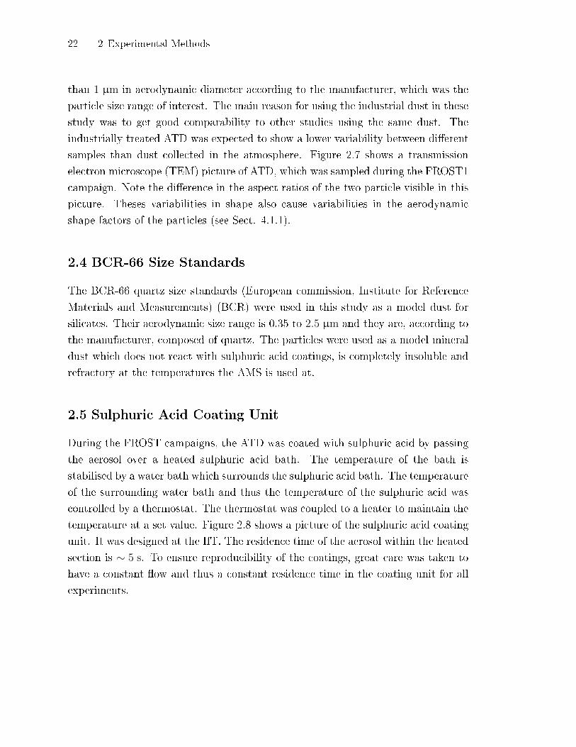
samples than dust collected in the atmosphere. Figure 2.7 shows a transmission
electron microscope (TEM) picture of ATD, which was sampled during the FROST1
campaign. Note the di�erence in the aspect ratios of the two particle visible in this
picture. Theses variabilities in shape also cause variabilities in the aerodynamic
shape factors of the particles (see Sect. 4.1.1).
2.4 BCR-66 Size Standards
The BCR-66 quartz size standards (European commission, Institute for Reference
Materials and Measurements) (BCR) were used in this study as a model dust for
silicates. Their aerodynamic size range is 0.35 to 2.5 µm and they are, according to
the manufacturer, composed of quartz. The particles were used as a model mineral
dust which does not react with sulphuric acid coatings, is completely insoluble and
refractory at the temperatures the AMS is used at.
2.5 Sulphuric Acid Coating Unit
During the FROST campaigns, the ATD was coated with sulphuric acid by passing
the aerosol over a heated sulphuric acid bath. The temperature of the bath is
stabilised by a water bath which surrounds the sulphuric acid bath. The temperature
of the surrounding water bath and thus the temperature of the sulphuric acid was
controlled by a thermostat. The thermostat was coupled to a heater to maintain the
temperature at a set value. Figure 2.8 shows a picture of the sulphuric acid coating
unit. It was designed at the IfT. The residence time of the aerosol within the heated
section is ∼ 5 s. To ensure reproducibility of the coatings, great care was taken to
have a constant �ow and thus a constant residence time in the coating unit for all
experiments.

2.5 Sulphuric Acid Coating Unit 23
Inner tube
Water bath surrounding the tube
Heated water input
Heater (below the table)
Sulphuric acid reservoir
(inside the inner tube)
Fig. 2.8: Sulphuric acid coating unit used during the FROST campaigns. The aerosolenters the coating unit in a glass tube and passes over a small heated sulphuric acid bath.To control the temperature, the sulphuric acid bath section is surrounded by a water bath.The temperature of the water is maintained by a heating unit below the table.)


3
Continuous Determination of AMS Detection Limits
The measurement of thin coatings on refractory particles as performed in this study
implies the necessity of detecting very small amounts of material. It is therefore
important to determine the smallest amount of material that can be reliably at-
tributed to the real signal. This amount is typically referred to as detection limit
(DL). It is commonly de�ned as three times the standard deviation of the signal
noise distribution σnoise plus a possible o�set µ of a blank measurement (Kellner
et al., 2004).
DL = 3× σnoise + µ (3.1)
This chapter gives an overview of methods used in the past to determine AMS
detetction limits and presents two new methods, whose applicability are tested. The
�rst method (Sect. 3.2.2) involves Bezier-smoothing-spline and is therefore referred
to as Bezier-method. It su�ers from some critical drawbacks which will be overcome
in the second, improved method presented in Sect. 3.2.3. The second new method
is based on local cubic interpolations and will be referred to as DL-cubic .
3.1 Classical Methods
In the recent AMS literature di�erent methods with di�erent strengths and weak-
nesses have been described to determine the limits of detection. The most commonly
used ones are summarised in the following sections.
3.1.1 Counting Statistics
A mathematically straight forward approach is to use the ion counting statistics of
the signal of a measurement through a particle �lter, thus only probing particle free

26 3 Continuous Determination of AMS Detection Limits
air. In the case of the AMS, this corresponds to the counting statistics error ∆Idiff
of the di�erence of the open Iopen and the closed Iclosed signal, as shown in Eq. (3.2).
∆Idiff =√Iopen + Iclosed (3.2)
A typical value of ∆Idiff for organics (recorded during the FROST1 campaign in
spring 2008 at the IfT in Leipzig) would be√3, 517, 000 + 3, 520, 000/
√132 = 231
This corresponds to a mass concentration DL of 0.14 µg/m3. The division by√132
is necessary to scale the counting statistics error for the whole measurement period,
which were 132 min, to a time resolution of 1 min. More values are shown in Tab.
3.8 in Sect. 3.2.8. The disadvantages of this method is that it wastes precious
measurement time while sampling through a particle �lter. Furthermore, it does
not take into account the electronic noise of the instrument. To get correct results,
the electronic noise needs to be determined separately. This proves di�cult in the
case of the AMS (see Sect. 3.2.8). Additional e�ects resulting from the processing
of the data, like baseline shifts, are not covered by this method as they add random
noise to the signal which is not directly linked to counting statistics.
3.1.2 Standard Deviation of Filter Measurements
Bahreini et al. (2003), Salcedo et al. (2006), Takegawa et al. (2005), Zhang et al.
(2005) and DeCarlo et al. (2006) used �ltered air measurements to determine the
detection limits of the AMS. The DL is estimated as three times the standard
deviation of a �lter measurement (3 × σfilter). The advantage of this method is
that the detection limits are determined experimentally and thus take into account
all e�ects which might be ignored when only taking into account the ion counting
statistics. A disadvantage is the need of �lter periods, which do not represent
the varying state of the instrument during regular measurements, where the closed
loadings can be increased due to the sampled aerosol (Drewnick et al., 2009).
3.1.3 Frequency Space Closed Signal Analysis
Crosier et al. (2007) avoid the need of �lter period measurements by using only the
closed signal of the instrument to determine the detection limits. They apply a Fast
Fourier Transformation (FFT) to the closed signal time series and use the relation
in Eq. (3.3) to determine the standard deviation of the noise σ. N and N ′ are the
number of points in the time and the frequency space1, respectively, and Iclosed is the
1The FFT decomposes a time series into periodic functions Cj exp−2πiωjt whose sum corre-
sponds to the original signal. The complex intensities Cj for every constituent frequency ωj yield
a spectrum in the frequency space.
3.1 Classical Methods 27
closed signal of the AMS. Note that the Fourier transformed spectrum is in complex
number space.
σ2 =2
N2
N ′−1∑n=1
|[FFT (Iclosed)]n|2 (3.3)
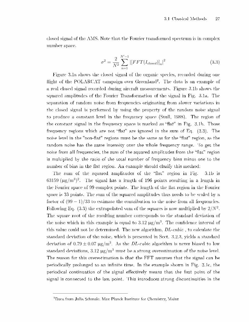
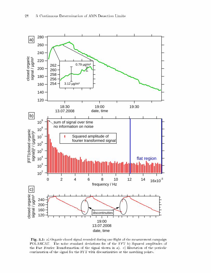
Figure 3.1a shows the closed signal of the organic species, recorded during one
�ight of the POLARCAT campaign over Greenland2. The data is an example of
a real closed signal recorded during aircraft measurements. Figure 3.1b shows the
squared amplitudes of the Fourier Transformation of the signal in Fig. 3.1a. The
separation of random noise from frequencies originating from slower variations in
the closed signal is performed by using the property of the random noise signal
to produce a constant level in the frequency space (Stull, 1988). The region of
the constant signal in the frequency space is marked as ��at� in Fig. 3.1b. Those
frequency regions which are not ��at� are ignored in the sum of Eq. (3.3). The
noise level in the �non-�at� regions must be the same as for the ��at� region, as the
random noise has the same intensity over the whole frequency range. To get the
noise from all frequencies, the sum of the squared amplitudes from the ��at� region
is multiplied by the ratio of the total number of frequency bins minus one to the
number of bins in the �at region. An example should clarify this method:
The sum of the squared amplitudes of the ��at� region in Fig. 3.1b is
63159 (µg/m3)2. The signal has a length of 196 points resulting in a length in
the Fourier space of 99 complex points. The length of the �at region in the Fourier
space is 33 points. The sum of the squared amplitudes thus needs to be scaled by a
factor of (99− 1)/33 to estimate the contribution to the noise from all frequencies.
Following Eq. (3.3) the extrapolated sum of the squares is now multiplied by 2/N2.
The square root of the resulting number corresponds to the standard deviation of
the noise which in this example is equal to 3.12 µg/m3. The con�dence interval of
this value could not be determined. The new algorithm, DL-cubic , to calculate the
standard deviation of the noise, which is presented in Sect. 3.2.3, yields a standard
deviation of 0.79± 0.07 µg/m3. As the DL-cubic algorithm is never biased to low
standard deviations, 3.12 µg/m3 must be a strong overestimation of the noise level.
The reason for this overestimation is that the FFT assumes that the signal can be
periodically prolonged to an in�nite time. In the example shown in Fig. 3.1c, the
periodical continuation of the signal e�ectively means that the �rst point of the
signal is connected to the last point. This introduces strong discontinuities in the
2Data from Julia Schmale, Max Planck Institute for Chemistry, Mainz
28 3 Continuous Determination of AMS Detection Limits
262260258256254
280
260
240
220
200
180
160
140
120
clos
ed o
rgan
icsi
gnal
/ µg
/m³
18:3013.07.2008
19:00 19:30date, time
240200160120
clos
ed o
rgan
icsi
gnal
/ µg
/m³
19:0013.07.2008date, time
102
103
104
105
106
107
108
109
|FF
T(c
lose
d or
gani
csi
gnal
)|²
/ (µg
/m³)
²
16x10-314121086420
frequency / Hz
flat region
Squared amplitude offourier transformed signal
sum of signal over timeno information on noise
a)
b)
3.12 µg/m³
0.79 µg/m³
c)
discontinuities
Fig. 3.1: a) Organic closed signal recorded during one �ight of the measurement campaignPOLARCAT. The noise standard deviations for of the FFT b) Squared amplitudes ofthe Fast Fourier Transformation of the signal shown in a). c) Illustation of the periodiccontinuation of the signal for the FFT with discontinuities at the matching points.

3.2 Noise Retrieval in Time Space 29
time series. These discontinuities contribute to the signal at every frequency in the
Fourier spectrum and thus arti�cially increases the estimated noise level.
As a typical AMS closed signal is not periodic, the possible applications of the
FFT-method to determine AMS detection limits is very limited. Crosier et al. (2007)
did not use the FFT-method to calculate absolute values of the detection limits but
only showed relative changes in the sum over the squares of the amplitudes of the �at
region in the frequency space. The authors do not explain how they dealt with the
non-periodicity of signals, but as the noise reduction method described in Crosier
et al. (2007) showed a very clear e�ect, the FFT-method showed a meaningfull
qualitative reduction of the noise.
3.1.4 Time Space Closed Signal Analysis
Drewnick et al. (2009) similar to Crosier et al. (2007) used the closed signal of the
AMS to determine the detection limits experimentally during regular instrument
operation. They directly calculated the standard deviation of the closed time series.
To avoid disturbances from long term variations in the AMS closed signal, only
periods during which the closed signal was constant were used to determine the
detection limits. This restricts the method to special situations for which the closed
signal is not disturbed and also limits the number of points that can be used for the
calculation. However, unlike the method described by Crosier, this method allows
for the calculation of absolute values of the DL.
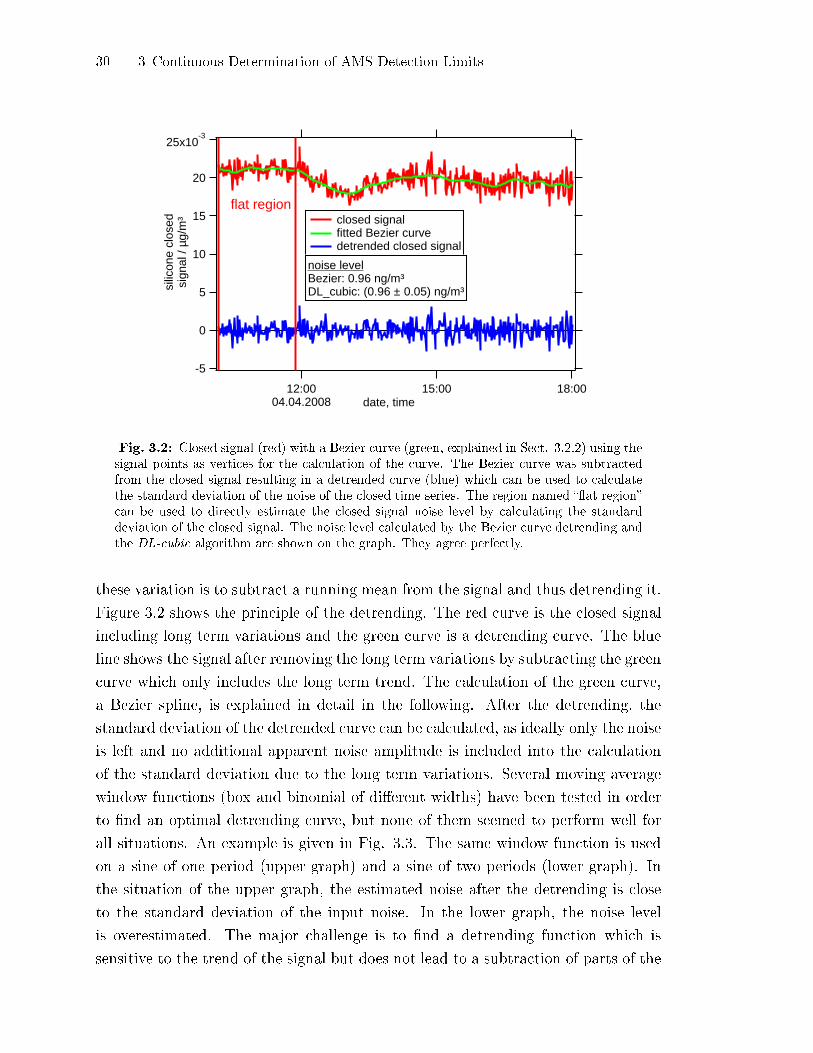
An example for a signal region to which this method could be applied is shown
in Fig. 3.2. The red curve is the closed signal which can be attributed to methyl
silicone. At the beginning of the curve the signal is �at and the standard deviation
of the signal in the �at region is equal to 0.85 ng/m3. The rest of the curve is not
suitable for this method to be applied, as the signal is not constant and thus the
signal itself would contribute to the standard deviation in addition to the noise.
In the next section, a method is presented which removes the trend of the signal,
ideally only leaving the random noise. In Fig. 3.2 this method is indicated by the
green curve which corresponds to the trend of the signal and the blue curve which
is the detrended signal.
3.2 Noise Retrieval in Time Space
3.2.1 Detrending of Closed Signals by Subtraction of a Running Mean
The major problem of the retrieval of detection limits from the noise level of the
closed signal are long term variations in this signal. The easiest way to eliminate
30 3 Continuous Determination of AMS Detection Limits
25x10-3
20
15
10
5
0
-5
silic
one
clos
edsi
gnal
/ µg
/m³
12:0004.04.2008
15:00 18:00date, time
flat region closed signal fitted Bezier curve detrended closed signal
noise levelBezier: 0.96 ng/m³DL_cubic: (0.96 ± 0.05) ng/m³
Fig. 3.2: Closed signal (red) with a Bezier curve (green, explained in Sect. 3.2.2) using thesignal points as vertices for the calculation of the curve. The Bezier curve was subtractedfrom the closed signal resulting in a detrended curve (blue) which can be used to calculatethe standard deviation of the noise of the closed time series. The region named ��at region�can be used to directly estimate the closed signal noise level by calculating the standarddeviation of the closed signal. The noise level calculated by the Bezier curve detrending andthe DL-cubic algorithm are shown on the graph. They agree perfectly.
these variation is to subtract a running mean from the signal and thus detrending it.
Figure 3.2 shows the principle of the detrending. The red curve is the closed signal
including long term variations and the green curve is a detrending curve. The blue
line shows the signal after removing the long term variations by subtracting the green
curve which only includes the long term trend. The calculation of the green curve,
a Bezier spline, is explained in detail in the following. After the detrending, the
standard deviation of the detrended curve can be calculated, as ideally only the noise
is left and no additional apparent noise amplitude is included into the calculation
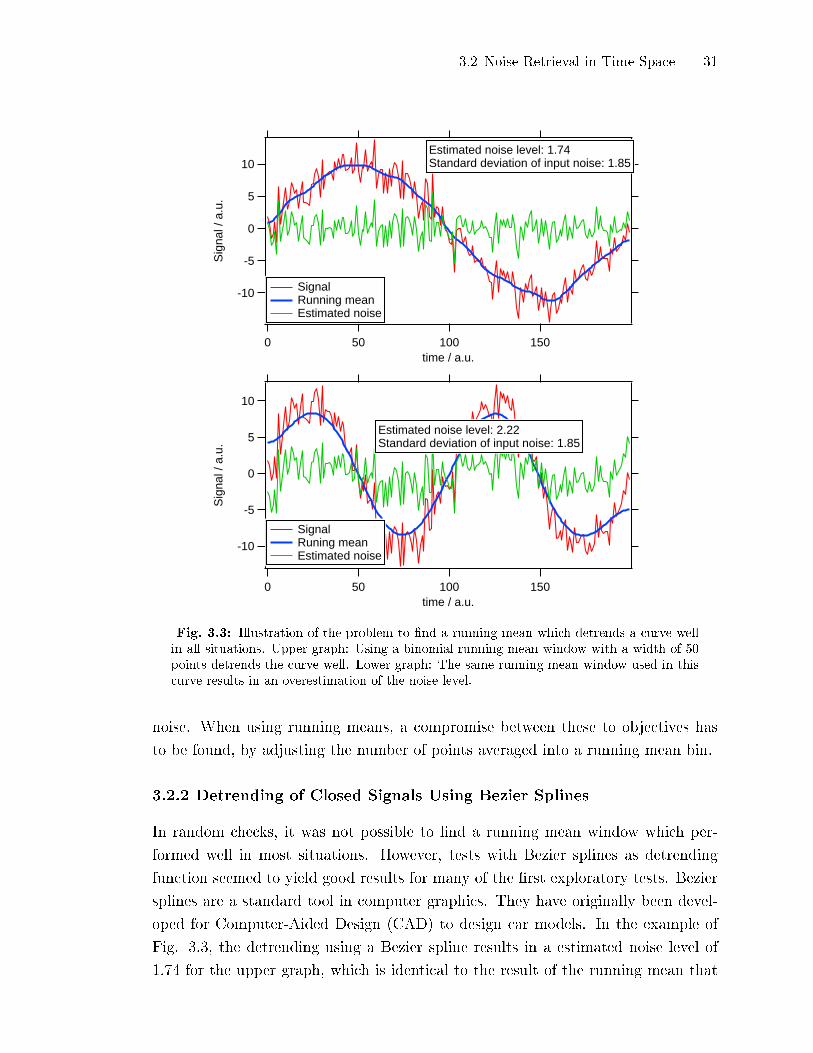
of the standard deviation due to the long term variations. Several moving average
window functions (box and binomial of di�erent widths) have been tested in order
to �nd an optimal detrending curve, but none of them seemed to perform well for
all situations. An example is given in Fig. 3.3. The same window function is used
on a sine of one period (upper graph) and a sine of two periods (lower graph). In
the situation of the upper graph, the estimated noise after the detrending is close
to the standard deviation of the input noise. In the lower graph, the noise level
is overestimated. The major challenge is to �nd a detrending function which is
sensitive to the trend of the signal but does not lead to a subtraction of parts of the
3.2 Noise Retrieval in Time Space 31
-10
-5
0
5
10
Sig
nal /
a.u
.
150100500time / a.u.
Estimated noise level: 1.74Standard deviation of input noise: 1.85
Signal Running mean Estimated noise
-10
-5
0
5
10
Sig
nal /
a.u
.
150100500time / a.u.
Signal Runing mean Estimated noise
Estimated noise level: 2.22Standard deviation of input noise: 1.85
Fig. 3.3: Illustration of the problem to �nd a running mean which detrends a curve wellin all situations. Upper graph: Using a binomial running mean window with a width of 50points detrends the curve well. Lower graph: The same running mean window used in thiscurve results in an overestimation of the noise level.
noise. When using running means, a compromise between these to objectives has
to be found, by adjusting the number of points averaged into a running mean bin.
3.2.2 Detrending of Closed Signals Using Bezier Splines
In random checks, it was not possible to �nd a running mean window which per-
formed well in most situations. However, tests with Bezier splines as detrending
function seemed to yield good results for many of the �rst exploratory tests. Bezier
splines are a standard tool in computer graphics. They have originally been devel-
oped for Computer-Aided Design (CAD) to design car models. In the example of
Fig. 3.3, the detrending using a Bezier spline results in a estimated noise level of
1.74 for the upper graph, which is identical to the result of the running mean that

32 3 Continuous Determination of AMS Detection Limits
worked �ne. For the lower graph, the detrending with the Bezier curve resulted in
an estmated noise level of 1.80. This is even closer to the standard deviation of the
input signal as for the running mean example. The Bezier splines were calculated
using the points of the signal as the vertices of the de�ning pologonal line. Normal
splines interpolate vertices, meaning that they create a smooth curve which passes
through all of its de�ning points. Bezier splines do not interpolate the vertices,
whcih in this thesis correspond to the signal points. They form curves which lie in
between the vertices and are only attracted towards these points. The major di�er-
ence between this method and a least square regression is that no model function
of the data is needed to obtain the curve. Figure 3.2 shows a closed signal with the
corresponding Bezier curve and the detrended closed noise signal. Mathematically
a Bezier curve or Bernstein-Bezier-curve ~r is de�ned as (see Bronstein et al., 2008,
p. 1007):
~r(z) =n∑i=0
Bi,n(z)~Pi, 0 ≤ z ≤ 1 (3.4)
with ~Pi being the polygon de�ning the curve, which in our case is the closed signal.
z is a parameter referring to the position on the curve with z = 0 being the starting
point and z = 1 the end point of the curve. The parameter z is not the x position
on a graph. Bi,n(z) are the Bernstein polynomials de�ned as:
Bi,n(z) =(ni
)zi(1− z)n−i, 0 ≤ z ≤ 1 (i = 0, 1, . . . , n) (3.5)
Calculating Bezier Curves: The de Casteljau Algorithm
The de�ning equation of the Bezier curves are shown for completeness. Calculating
Bezier curves by directly using Eq. (3.4) is unusual. Typically special algorithms
are used to determine Bezier splines. In this work, the calculation of the Bezier
curves is performed using the de-Casteljau-algorithm, developed by Paul de Faget de
Casteljau in the early 1960's at Citroën. A description of the de-Casteljau-algorithm
is given at Schwarz and Köckler (2006). An very comprehensive description is given
at Wikipedia (2011). The text of the original patent (de Casteljau, 1959) was not
available. As the de-Casteljau-algorithm is not commonly applied in the �eld of
aerosol science, it is described here in more details referring to Fig. 3.4.
The �gure shows the construction of one single point of a Bezier curve. In a), the
blue polygonal line ~Pi from Eq. (3.4) corresponds to the signal to be detrended. It is
used to de�ne the Bezier curve. The �rst step of the construction is to determine the
red points which are situated half way between the blue vertices ~Pi. These points
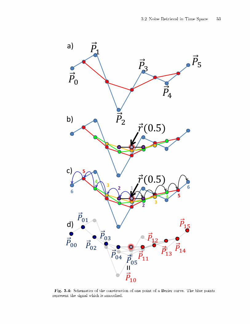
3.2 Noise Retrieval in Time Space 33
𝑟 (0.5)
𝑃0
𝑃1
𝑃2
𝑃3
𝑃4
𝑃5
𝑃00
𝑃01
𝑃02 𝑃03
𝑃04 𝑃05 𝑃11
𝑃12
𝑃13 𝑃14
𝑃15
a)
b)
d)
𝑃10
=
𝑟 (0.5) c)
1 2 3
4
5
6
2 3
4 5
6
Fig. 3.4: Schematics of the construction of one point of a Bezier curve. The blue pointsrepresent the signal which is smoothed.
34 3 Continuous Determination of AMS Detection Limits
form a new polygonal line which has one point less than the original polygonal line~Pi. Similar to the constrauction of the red polygonal, again, the points situated half
way between the points can be used to construct a new polygonal. This polygonal
has one point less than the red polygonal. It is marked in green in Fig. 3.4b. By
iterating the procedure, the degree of the polygonal lines is reduced by one in every
iteration step until only one single point is left. This is the �rst point ~r(0.5) of the
Bezier curve.
Using points which were determined during the calculation of the �rst point, two
additional points on each side of the �rst point can be calculated. The procedure to
�nd these points is illustrated in Fig. 3.4c. The �rst vortex de�ning the new point
on each side of ~r(0.5) is ~r(0.5) itself. The second de�ning vortex is the purple point
to left of ~r(0.5). It is the closest point on the left of ~r(0.5) which is connected to
this point by a line. The third vortex is obtained by again moving to the left of the
second vortex allong the yellow connecting line to the yellow point. By moving to
the left allong the connecting lines, all the new vertices de�ning the point on the
left are determined. The last vortex is the �rst point of the signal (blue point on the
left). The same procedure can be used on the left of ~r(0.5) to obtain the de�ning
vertices for the new point on the right. In Fig. 3.4d, the two new polygonal lines are
marked in blue and red, respectively and share the point ~r(0.5). These two polygonal
lines can be used to calculate two further points ~r(0.25) and ~r(0.75) on each side
of ~r(0.5) using the same procedure that was used to determine ~r(0.5). By further
iterating this procedure, additional points of the Bezier spline can be calculated,
until the desired precision is reached. In every iteration step k, 2k new points are
obtaned. In this work the desired number of points was the lowest possible number
which was higher than the number of signal points which were smoothed. Before
subtraction from the signal, the Bezier curve needs to be calculated at the positions
of the points of the signal. This was done using linear interpolation.
Test of the Bezier Detrending Method
Prior to its application to determine detection limits, the Bezier detrending method
was validated for a set of realistic signals. These tests showed that the simple
Bezier curves do often not properly detrend the noise and some modi�cations are
proposed to improve the detrending. However, the Bezier curves, although being an
improvement compared to simple moving averages, proved to be inappropriate for
a reproducible detrending. Hence a di�erent method is developed in Sect. 3.2.3.
To test if a signal detrended with a Bezier curve does really correspond to the noise
of the curve, this method was tested on arti�cial, generated signals with Gaussian
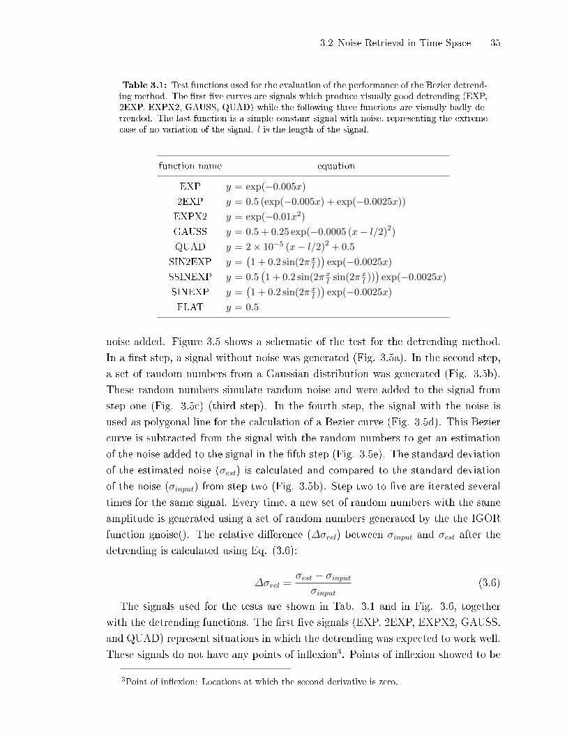
3.2 Noise Retrieval in Time Space 35
Table 3.1: Test functions used for the evaluation of the performance of the Bezier detrend-ing method. The �rst �ve curves are signals which produce visually good detrending (EXP,2EXP, EXPX2, GAUSS, QUAD) while the following three functions are visually badly de-trended. The last function is a simple constant signal with noise, representing the extremecase of no variation of the signal. l is the length of the signal.
function name equation
EXP
2EXP
EXPX2
GAUSS
QUAD
SIN2EXP
SSINEXP
SINEXP
FLAT
y = exp(−0.005x)y = 0.5 (exp(−0.005x) + exp(−0.0025x))y = exp(−0.01x2)y = 0.5 + 0.25 exp(−0.0005 (x− l/2)2)y = 2× 10⁻⁵ (x− l/2)2 + 0.5
y =(1 + 0.2 sin(2π xl )
)exp(−0.0025x)
y = 0.5(1 + 0.2 sin(2π xl sin(2π
xl )))exp(−0.0025x)
y =(1 + 0.2 sin(2π xl )
)exp(−0.0025x)
y = 0.5
noise added. Figure 3.5 shows a schematic of the test for the detrending method.
In a �rst step, a signal without noise was generated (Fig. 3.5a). In the second step,
a set of random numbers from a Gaussian distribution was generated (Fig. 3.5b).
These random numbers simulate random noise and were added to the signal from
step one (Fig. 3.5c) (third step). In the fourth step, the signal with the noise is
used as polygonal line for the calculation of a Bezier curve (Fig. 3.5d). This Bezier
curve is subtracted from the signal with the random numbers to get an estimation
of the noise added to the signal in the �fth step (Fig. 3.5e). The standard deviation
of the estimated noise (σest) is calculated and compared to the standard deviation
of the noise (σinput) from step two (Fig. 3.5b). Step two to �ve are iterated several
times for the same signal. Every time, a new set of random numbers with the same
amplitude is generated using a set of random numbers generated by the the IGOR
function gnoise(). The relative di�erence (∆σrel) between σinput and σest after the
detrending is calculated using Eq. (3.6):
∆σrel =σest − σinput
σinput(3.6)
The signals used for the tests are shown in Tab. 3.1 and in Fig. 3.6, together
with the detrending functions. The �rst �ve signals (EXP, 2EXP, EXPX2, GAUSS,
and QUAD) represent situations in which the detrending was expected to work well.
These signals do not have any points of in�exion3. Points of in�exion showed to be
3Point of in�exion: Locations at which the second derivative is zero.

36 3 Continuous Determination of AMS Detection Limits
-10-505
10
150100500time / arbitrary units
-10-505
10
-10-505
10
-10-505
10
-10-505
10
ampl
itude
/ ar
bitr
ary
units
Signal
Gaussian noise
Signal plus noise
Bezier curve
Estimated noise
a)
b)
c)
d)
e)
Fig. 3.5: a) Generated signal. b) Generated Gaussian noise. c) Generated signal withgenerated nosie added. d) Curve from �c)� with Bezier curve. e) Estimated noise after thedetrending using the Bezier curve.
the most di�cult feature to detrend in the �rst tests, especially in situations when
only few signal points were available per in�exion point. An example of a curve
including in�exion points for which the detrending works �ne is the curve in Fig.
3.5. In this case, 50 signal points were available for every in�exion point. On each
of the graphs ∆σrel is indicated for the special set of random numbers added to the
function shown in the graph. For all of these �simple� cases, the noise level was
underestimated.
Each test function from Tab. 3.1 was used 20 times with di�erent sets of random
numbers. The estimated noise levels were compared to the input noise levels. For
each function, ∆σrel was calculated for every set of random numbers. Figure 3.7
summarises the averages of the relative deviations ∆σrel together with the standard

3.2 Noise Retrieval in Time Space 37
1.0
0.8
0.6
0.4
0.2
0.0
a.u.
403020100x
relative error: -5 %
b)
2EXP
1.0
0.8
0.6
0.4
0.2
0.0
a.u.
403020100x
signal Bezier trend detrended signal
relative error: -14 %
a)
EXP
1.0
0.8
0.6
0.4
0.2
0.0
a.u.
403020100x
relative error: -26 %
c)
EXPX2
0.6
0.4
0.2
0.0a.
u.
403020100x
relative error: -12 %
d)
GAUSS
0.5
0.4
0.3
0.2
0.1
0.0
a.u.
403020100x
relative error: -13 %
e)
QUAD
0.5
0.4
0.3
0.2
0.1
0.0
a.u.
403020100x
relative error: 56 %
f)
SIN2EXP
1.0
0.8
0.6
0.4
0.2
0.0
a.u.
403020100x
relative error: 35 %
h)
SINEXP
0.5
0.4
0.3
0.2
0.1
0.0
a.u.
403020100x
relative error: 161 %
g)
SSINEXP
Fig. 3.6: Generated signals with normal noise with a standard deviation of 0.01. Each�gure shows the signal together with an attempted detrending with a Bezier curve calculateddirectly using the signal points as vertices. The signal equations are listed in Tab. 3.1. Therelative errors were calculated using Eq. (3.6)
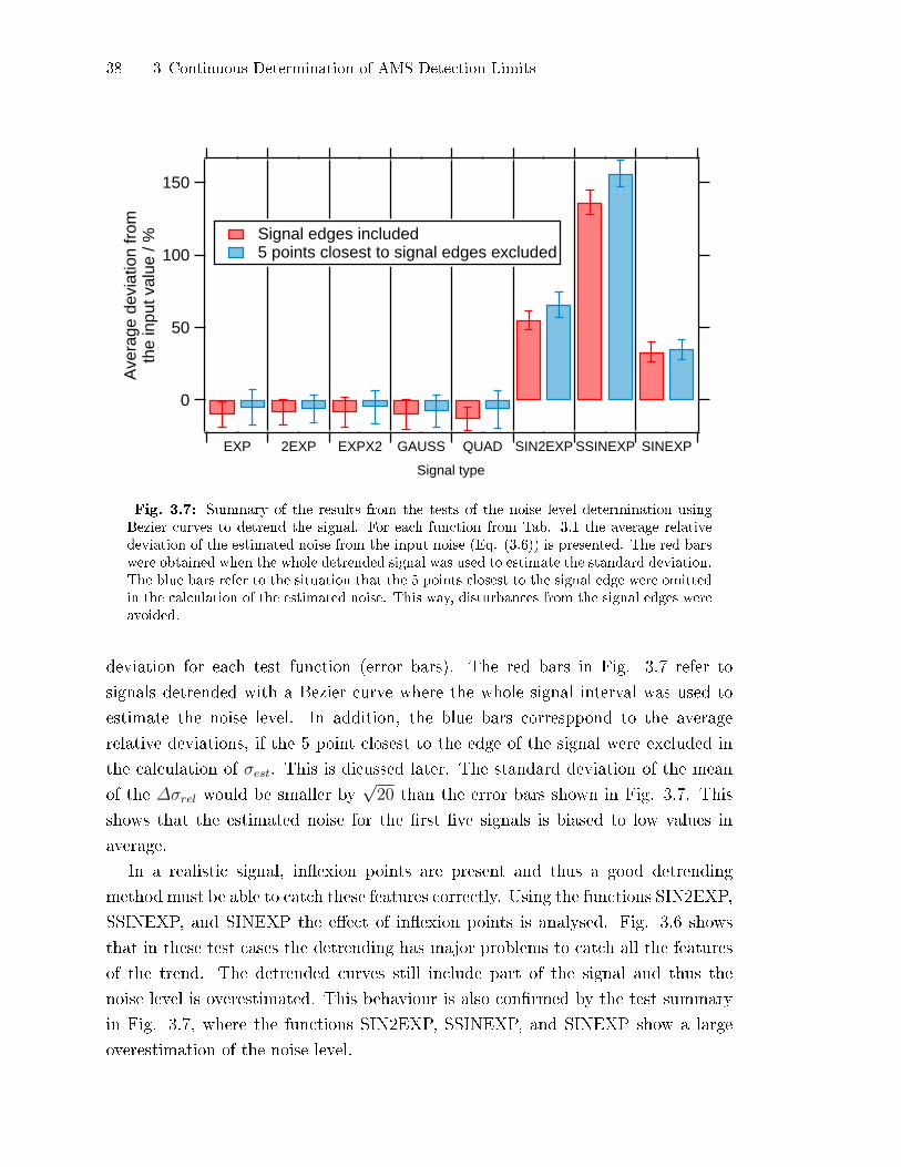
38 3 Continuous Determination of AMS Detection Limits
150
100
50
0
Ave
rage
dev
iatio
n fr
omth
e in
put v
alue
/ %
EXP 2EXP EXPX2 GAUSS QUAD SIN2EXP SSINEXP SINEXP
Signal type
1.0
0.8
0.6
0.4
0.2
0.0
6420
Signal edges included 5 points closest to signal edges excluded
Fig. 3.7: Summary of the results from the tests of the noise level determination usingBezier curves to detrend the signal. For each function from Tab. 3.1 the average relativedeviation of the estimated noise from the input noise (Eq. (3.6)) is presented. The red barswere obtained when the whole detrended signal was used to estimate the standard deviation.The blue bars refer to the situation that the 5 points closest to the signal edge were omittedin the calculation of the estimated noise. This way, disturbances from the signal edges wereavoided.
deviation for each test function (error bars). The red bars in Fig. 3.7 refer to
signals detrended with a Bezier curve where the whole signal interval was used to
estimate the noise level. In addition, the blue bars corresppond to the average
relative deviations, if the 5 point closest to the edge of the signal were excluded in
the calculation of σest. This is dicussed later. The standard deviation of the mean
of the ∆σrel would be smaller by√20 than the error bars shown in Fig. 3.7. This
shows that the estimated noise for the �rst �ve signals is biased to low values in
average.
In a realistic signal, in�exion points are present and thus a good detrending
method must be able to catch these features correctly. Using the functions SIN2EXP,
SSINEXP, and SINEXP the e�ect of in�exion points is analysed. Fig. 3.6 shows
that in these test cases the detrending has major problems to catch all the features
of the trend. The detrended curves still include part of the signal and thus the
noise level is overestimated. This behaviour is also con�rmed by the test summary
in Fig. 3.7, where the functions SIN2EXP, SSINEXP, and SINEXP show a large
overestimation of the noise level.

3.2 Noise Retrieval in Time Space 39
Attempts to Optimise the Bezier Detrending Method
Reduction of disturbances from the signal edges
The �rst test series show that the straightforward calculation of the Bezier curves
su�ers from two issues. First, for signals without any in�exion points (Fig. 3.6a-e)
the method results in an underestimation of the noise level. Second, for signals with
in�exion points of a few signal points (Fig. 3.6f-h) the noise is overestimated. The
underestimation can partially be explained by the property of the Bezier curves to
extrapolate the vertices at the edge of the curve. Furthermore, vertices close to the
edge attract the curve much stronger than those in the middle of the signal. To
reduce this e�ect, the noise level of the 8 signals introduced above was calculated
without using the �ve points closest to the signal edges on each side of the signal,
respectively. The blue bars in Fig. 3.7 show the average results of this modi�ed
method. For all signals which underestimated the noise level, this method results in
an improvement. However, as expected, those signals that tend to overestimate the
noise level become even worse.
A drawback of ignoring the points at the edge of the signal is that the information
of these points is lost. Therefore, as an alternative method, the signal was extrapo-
lated linearly on each side prior to the calculation of the Bezier curve. However, the
standard deviation was only calculated for the part of the detrended curve which
originates from the signal. The extrapolation was done by calculating a linear �tting
curve through the 10 points closest to the signal edges. The number of extrapolated
points was 20. This extrapolation prevents the edges of the signal to be the edges
of the Bezier curve, reducing the e�ect of the underestimation similarly to ignoring
the edges. Fig. 3.8 shows an example of a prolonged signal with the corresponding
detrending. In this speci�c case, the underestimation was reduced from −28 % to
−24 %.
Optimisation of the locations of the vertices
Despite the elimination of the boundary e�ects, the noise level is still systematically
underestimated for the �ve �rst test cases. Furthermore, the existance of in�ex-
ion points in the functions SIN2EXP, SSIN2EXP, and SINEXP resulted in drastic
overestimations. The underestimation can be lowered by decreasing the number of
vertices used for the Bezier curve. This e�ectively reduces the degree n (Eq. (3.4))
of the polynomial used to interpolate the curve an thus it is less sensitive to the short
variations of the curve. However, with the reduction of the number of vertices, the
signal points can no longer be used as vertices. It is thus necessary to determine
new vertices which can afterwards be �tted by using standard �tting routines. The

40 3 Continuous Determination of AMS Detection Limits
50403020100a.u.
9080706050403020100a.u.
generated signal detrended signal Bezier fit
a) b)
Fig. 3.8: a) Generated signal with Bezier detrending. The standard deviation is under-estimated by 28 % b) Generated signal with linearly extrapolated edges which reduce theunderestimation of the noise standard deviation to 24 %.
objective is to improve the detrending of signals with in�exion points along with
reducing the degree of freedom of the curve. Therefore, the vertices must be set at
those x-values at which the major changes of the signal take place. These are the
locations of the roots4 of the derivatives of the signal.
In practice, the calculation was done as follows: In the �rst step a Bezier curve
was calculated from the signal as described above to get a rough estimation of
the real signal. This Bezier curve was used to calculate the roots of the �rst, the
second, and the third derivative. These roots were used as the x-positions of the
new vertices. The y-values of the vertices were initialised with the �rst value of
the signal. The �tting algorithm of Igor (WaveMetrics, Inc. Lake Oswego, Oregon,
USA) quickly converges to a good approximation of the curve. Nevertheless, the
Bezier curve needs to be calculated several times, which causes the �tting to take
up to two minutes for a signal of only 50 points on an Intel R© CoreTM
2 Duo CPU with
two 2 MHz processor cores. If the signal is composed of 400 points, the computation
time expense is raised to up to a quarter of an hour on the used computer.
The method using a Bezier �tting function was tested using optionally the x-
locations of the �rst three derivatives, the �rst two derivatives or the second and
the third derivative. For all three choices of the vertices's x-coordinates the signal
edges were used with and without a linear extrapolation of the signal edges. Table
3.2 shows a compilation of the e�ects of the combination of di�erent optimisation
attempts. Only the functions FLAT, as the extreme case for underestimation e�ects,
4Roots of a function: Positions where the function is zero.
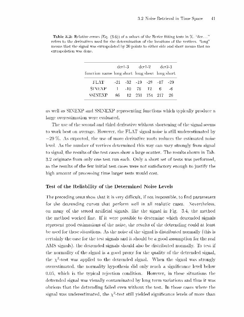
3.2 Noise Retrieval in Time Space 41
Table 3.2: Relative errors (Eq. (3.6)) of a subset of the Bezier �tting tests in %. �der. . . �refers to the derivatives used for the determination of the locations of the vertices. �long�means that the signal was extrapolated by 20 points to either side and short means that noextrapolation was done.
der1-3 der1-2 der2-3
function name long short long short long short
FLAT -21 -32 -19 -28 -17 -29
SINEXP 1 -10 76 12 6 -6
SSINEXP 86 -12 231 154 217 26
as well as SINEXP and SSINEXP representing functions which typically produce a
large overestimation were evaluated.
The use of the second and third derivative without shortening of the signal seems
to work best on average. However, the FLAT signal noise is still underestimated by
−29 %. As expected, the use of more derivative roots reduces the estimated noise
level. As the number of vertices determined this way can vary strongly from signal
to signal, the results of the test cases show a large scatter. The results shown in Tab.
3.2 originate from only one test run each. Only a short set of tests was performed,
as the results of the few initial test cases were not satisfactory enough to justify the
high amount of processing time larger tests would cost.
Test of the Reliability of the Determined Noise Levels
The preceding tests show that it is very di�cult, if not impossible, to �nd parameters
for the detrending curves that perform well in all realistic cases. Nevertheless,
on many of the tested arti�cial signals, like the signal in Fig. 3.4, the method
the method worked �ne. If it were possible to determine which detrended signals
represent good estimations of the noise, the results of the detrending could at least
be used for these situations. As the noise of the signal is distributed normally (this is
certainly the case for the test signals and it should be a good assumption for the real
AMS signals), the detrended signals should also be distributed normally. To test if
the normality of the signal is a good proxy for the quality of the detrended signal,
the χ2-test was applied to the detrended signal. When the signal was strongly
overestimated, the normality hypothesis did only reach a signi�cance level below
0.05, which is the typical rejection condition. However, in these situations the
detrended signal was visually contaminated by long term variations and thus it was
obvious that the detrending failed even without the test. In those cases where the
signal was underestimated, the χ2-test still yielded signi�cance levels of more than
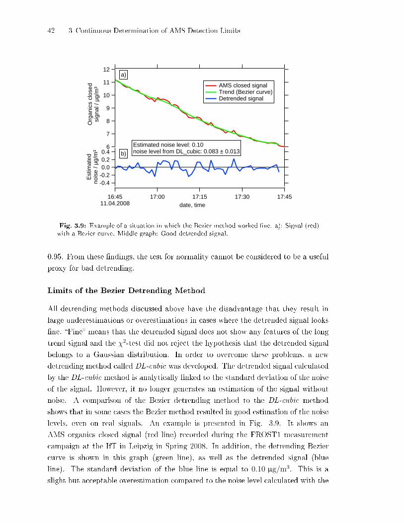
42 3 Continuous Determination of AMS Detection Limits
12
11
10
9
8
7
6
Org
anic
s cl
osed
sign
al /
µg/m
³
16:4511.04.2008
17:00 17:15 17:30 17:45date, time
-0.4-0.20.00.20.4
Est
imat
edno
ise
/ µg/
m³
AMS closed signal Trend (Bezier curve) Detrended signal
Estimated noise level: 0.10noise level from DL_cubic: 0.083 ± 0.013
a)
b)
Fig. 3.9: Example of a situation in which the Bezier method worked �ne. a): Signal (red)with a Bezier curve. Middle graph: Good detrended signal.
0.95. From these �ndings, the test for normality cannot be considered to be a useful
proxy for bad detrending.
Limits of the Bezier Detrending Method
All detrending methods discussed above have the disadvantage that they result in
large underestimations or overestimations in cases where the detrended signal looks
�ne. �Fine� means that the detrended signal does not show any features of the long
trend signal and the χ2-test did not reject the hypothesis that the detrended signal
belongs to a Gaussian distribution. In order to overcome these problems, a new
detrending method called DL-cubic was developed. The detrended signal calculated
by the DL-cubic method is analytically linked to the standard deviation of the noise
of the signal. However, it no longer generates an estimation of the signal without
noise. A comparison of the Bezier detrending method to the DL-cubic method
shows that in some cases the Bezier method resulted in good estimation of the noise
levels, even on real signals. An example is presented in Fig. 3.9. It shows an
AMS organics closed signal (red line) recorded during the FROST1 measurement
campaign at the IfT in Leipzig in Spring 2008. In addition, the detrending Bezier
curve is shown in this graph (green line), as well as the detrended signal (blue
line). The standard deviation of the blue line is equal to 0.10 µg/m3. This is a
slight but acceptable overestimation compared to the noise level calculated with the

3.2 Noise Retrieval in Time Space 43
5.4
5.2
5.0
4.8
4.6
Org
anic
s cl
osed
sign
al /
µg/m
³
13:0014.04.2008
14:00 15:00date, time
-0.2-0.10.00.10.2
DL_
cubi
cde
tren
ded
sign
al /
µg/m
³
-0.2-0.10.00.10.2
Bez
ier
estim
ated
nois
e / µ
g/m
³ AMS closed signal trend (Bezier curve) poorly detrended signal detrended signal with DL_cubic
Fig. 3.10: Example of a situation in which the Bezier method worked bad. Upper graph:Signal (red) with a Bezier curve. Middle graph: Badly detrended signal. Lower Graph:Alternative detreding using the DL-cubic .
DL-cubic-method (0.083± 0.013 µg/m3). However, Fig. 3.10 shows the organics
closed signal of the AMS, recorded three days later during the same campaign. For
this curve, the Bezier detrending fails. The noise level is estimated to 0.071 µg/m3
while the DL-cubic yields a noise level of 0.035± 0.003 µg/m3. In addition to the
Bezier detrending, the detrended signal using the DL-cubic method is shown in the
lower graph. In contrast to the detrended signals of the Bezier method, it does not
correspond to the noise of the curve. However, it does not show the long term trends
of the signal, which are visible for the Bezier detrended signal.
In favourable situations, the Bezier detrending method can thus give good approx-
imations of the noise and in addition yield an approximation of the signal without
noise. The drawback of the method is the inability to determine when the Bezier
method worked �ne and when it failed. Nevertheless, the trends of the Bezier curve
can be used as good approximations of the real signals, if the noise level was correctly
determined. If this is the case needs to be determined using an independent method
to determine the noise level. However, �nding the signal without noise was not the
goal of this work. If the noise level is already known, mathematically more powerful
methods to determine the trend of a signal exist, without knowing the exact �tting

44 3 Continuous Determination of AMS Detection Limits
-2 -1 0 1 2 -2 -1 0 1 2
cubic fit to 4 closest points ideal signal interpolated point
cubic fit to 4 closest points signal with noise interpolated point
𝑓𝑖−2
𝑓𝑖 ≈ ℎ𝑖 𝑓𝑖−1
𝑓𝑖+2
𝑓𝑖+1
𝐹𝑖−1
𝐹𝑖+1
𝐹𝑖−2
𝐹𝑖
𝐹𝑖+2
𝐻𝑖
𝐹𝑖 −𝐻𝑖 = 𝐸𝑖
𝑓(𝑡
𝑖) 𝐹
(𝑡𝑖 )
𝑡𝑖 𝑡𝑖
Fig. 3.11: Local �t of a signal by a third order polynomial with the centre point omitted.The green points hi and Hi mark the interpolated central points. For the ideal signal f (leftgraph) it is approximately equal to the central point of the curve. In the case of a real signalwith noise F , Fi and Hi di�er by Ei.
function. An example would be Generalised Additive Models Wood (2006). For the
needs of this thesis, the Bezier detrending method is thus not an optimal choice and
therefore the new method DL-cubic was developed and is presented in the following
section.
3.2.3 Derivation of a Cubic Detrending Algorithm
In the following sections an algorithm for the determination of the noise level of a
curve is presented and its application to AMS detection limits is demonstrated. The
algorithm was named DL-cubic as it is mainly used to calculate detection limits of
the AMS using a detrending of the AMS closed signal by a local signal interpolation
with a cubic function. Originally, the algorithm was designed to automatically �nd
locations of curves, which cause problems to the Bezier algorithm, because the signal
abruptly changes its direction. For this purpose, the local deviation of the curve
from a cubic function was probed. The derivation from a cubic function was used
as a cubic function is the �rst polynomial which includes an in�exion point. After a
mathematical analysis, it was possible to determine an analytical relation between
the probed value and the noise level itself.
The main condition for the application of the DL-cubic algorithm is that the time
scale of variation of the signal is clearly longer than the time scale of the noise. The
time scale of the noise is equal to the sampling interval. Furthermore, it must be
possible to locally approximate the signal by a polynomial of the third order. In the
AMS the long term variations of the signal are mainly caused by substances accu-
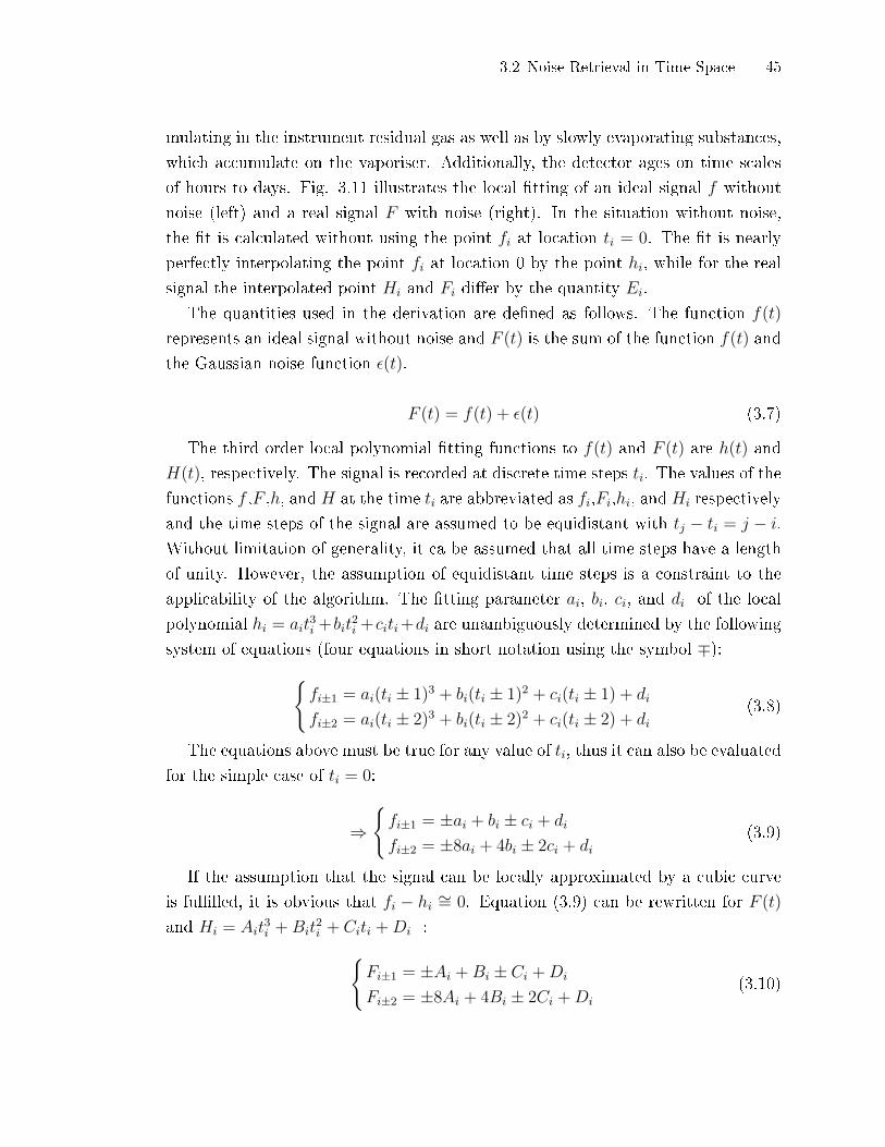
3.2 Noise Retrieval in Time Space 45
mulating in the instrument residual gas as well as by slowly evaporating substances,
which accumulate on the vaporiser. Additionally, the detector ages on time scales
of hours to days. Fig. 3.11 illustrates the local �tting of an ideal signal f without
noise (left) and a real signal F with noise (right). In the situation without noise,
the �t is calculated without using the point fi at location ti = 0. The �t is nearly
perfectly interpolating the point fi at location 0 by the point hi, while for the real
signal the interpolated point Hi and Fi di�er by the quantity Ei.
The quantities used in the derivation are de�ned as follows. The function f(t)
represents an ideal signal without noise and F (t) is the sum of the function f(t) and
the Gaussian noise function ε(t).
F (t) = f(t) + ε(t) (3.7)
The third order local polynomial �tting functions to f(t) and F (t) are h(t) and
H(t), respectively. The signal is recorded at discrete time steps ti. The values of the
functions f ,F ,h, and H at the time ti are abbreviated as fi,Fi,hi, and Hi respectively
and the time steps of the signal are assumed to be equidistant with tj − ti = j − i.Without limitation of generality, it ca be assumed that all time steps have a length
of unity. However, the assumption of equidistant time steps is a constraint to the
applicability of the algorithm. The �tting parameter ai, bi, ci, and di of the local
polynomial hi = ait3i +bit
2i +citi+di are unambiguously determined by the following
system of equations (four equations in short notation using the symbol ∓):{fi±1 = ai(ti ± 1)3 + bi(ti ± 1)2 + ci(ti ± 1) + di
fi±2 = ai(ti ± 2)3 + bi(ti ± 2)2 + ci(ti ± 2) + di(3.8)
The equations above must be true for any value of ti, thus it can also be evaluated
for the simple case of ti = 0:
⇒
{fi±1 = ±ai + bi ± ci + di
fi±2 = ±8ai + 4bi ± 2ci + di(3.9)
If the assumption that the signal can be locally approximated by a cubic curve
is ful�lled, it is obvious that fi − hi ∼= 0. Equation (3.9) can be rewritten for F (t)
and Hi = Ait3i +Bit
2i + Citi +Di :{
Fi±1 = ±Ai +Bi ± Ci +Di
Fi±2 = ±8Ai + 4Bi ± 2Ci +Di
(3.10)
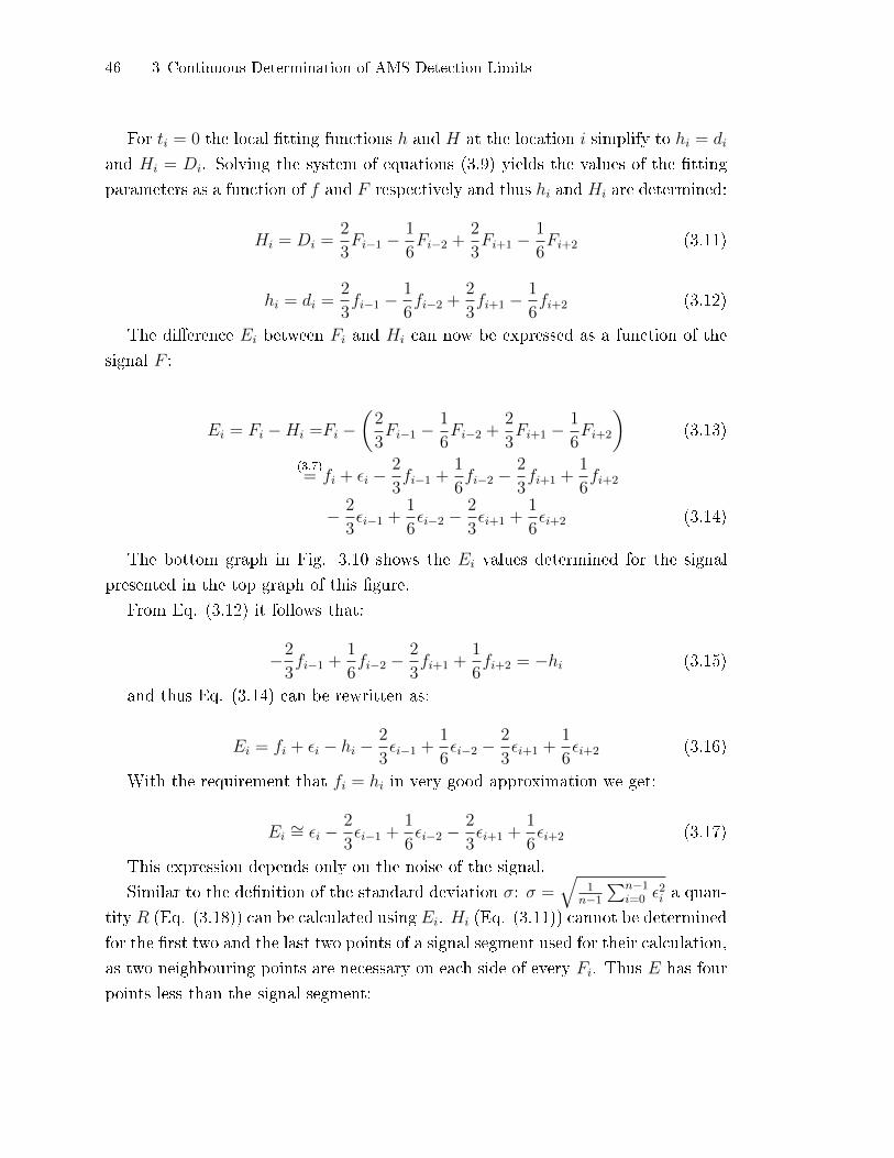
46 3 Continuous Determination of AMS Detection Limits
For ti = 0 the local �tting functions h and H at the location i simplify to hi = di
and Hi = Di. Solving the system of equations (3.9) yields the values of the �tting
parameters as a function of f and F respectively and thus hi and Hi are determined:
Hi = Di =2
3Fi−1 −
1
6Fi−2 +
2
3Fi+1 −
1
6Fi+2 (3.11)
hi = di =2
3fi−1 −
1
6fi−2 +
2
3fi+1 −
1
6fi+2 (3.12)
The di�erence Ei between Fi and Hi can now be expressed as a function of the
signal F :
Ei = Fi −Hi =Fi −(2
3Fi−1 −
1
6Fi−2 +
2
3Fi+1 −
1
6Fi+2
)(3.13)
(3.7)= fi + εi −
2
3fi−1 +
1
6fi−2 −
2
3fi+1 +
1
6fi+2
− 2
3εi−1 +
1
6εi−2 −
2
3εi+1 +
1
6εi+2 (3.14)
The bottom graph in Fig. 3.10 shows the Ei values determined for the signal
presented in the top graph of this �gure.
From Eq. (3.12) it follows that:
−2
3fi−1 +
1
6fi−2 −
2
3fi+1 +
1
6fi+2 = −hi (3.15)
and thus Eq. (3.14) can be rewritten as:
Ei = fi + εi − hi −2
3εi−1 +
1
6εi−2 −
2
3εi+1 +
1
6εi+2 (3.16)
With the requirement that fi = hi in very good approximation we get:
Ei ∼= εi −2
3εi−1 +
1
6εi−2 −
2
3εi+1 +
1
6εi+2 (3.17)
This expression depends only on the noise of the signal.
Similar to the de�nition of the standard deviation σ: σ =√
1n−1
∑n−1i=0 ε
2i a quan-
tity R (Eq. (3.18)) can be calculated using Ei. Hi (Eq. (3.11)) cannot be determined
for the �rst two and the last two points of a signal segment used for their calculation,
as two neighbouring points are necessary on each side of every Fi. Thus E has four
points less than the signal segment:
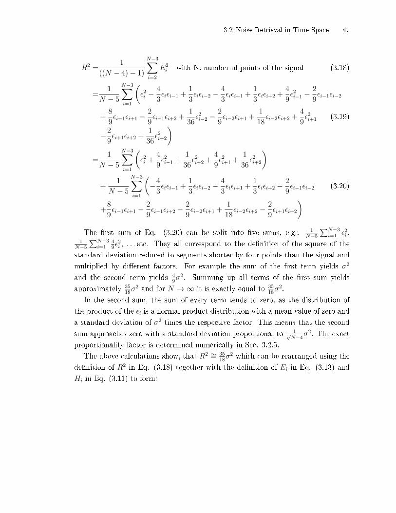
3.2 Noise Retrieval in Time Space 47
R2 =1
((N − 4)− 1)
N−3∑i=2
E2i with N: number of points of the signal (3.18)
=1
N − 5
N−3∑i=1
(ε2i −
4
3εiεi−1 +
1
3εiεi−2 −
4
3εiεi+1 +
1
3εiεi+2 +
4
9ε2i−1 −
2
9εi−1εi−2
+8
9εi−1εi+1 −
2
9εi−1εi+2 +
1
36ε2i−2 −
2
9εi−2εi+1 +
1
18εi−2εi+2 +
4
9ε2i+1 (3.19)
−2
9εi+1εi+2 +
1
36ε2i+2
)=
1
N − 5
N−3∑i=1
(ε2i +
4
9ε2i−1 +
1
36ε2i−2 +
4
9ε2i+1 +
1
36ε2i+2
)
+1
N − 5
N−3∑i=1
(−4
3εiεi−1 +
1
3εiεi−2 −
4
3εiεi+1 +
1
3εiεi+2 −
2
9εi−1εi−2 (3.20)
+8
9εi−1εi+1 −
2
9εi−1εi+2 −
2
9εi−2εi+1 +
1
18εi−2εi+2 −
2
9εi+1εi+2
)The �rst sum of Eq. (3.20) can be split into �ve sums, e.g.: 1
N−5∑N−3
i=1 ε2i ,1
N−5∑N−3
i=149ε2i , . . . etc. They all correspond to the de�nition of the square of the
standard deviation reduced to segments shorter by four points than the signal and
multiplied by di�erent factors. For example the sum of the �rst term yields σ2
and the second term yields 49σ2. Summing up all terms of the �rst sum yields
approximately 3518σ2 and for N →∞ it is exactly equal to 35
18σ2.
In the second sum, the sum of every term tends to zero, as the distribution of
the product of the εi is a normal product distribution with a mean value of zero and
a standard deviation of σ2 times the respective factor. This means that the second
sum approaches zero with a standard deviation proportional to 1√N−4σ
2. The exact
proportionality factor is determined numerically in Sec. 3.2.5.
The above calculations show, that R2 ∼= 3518σ2 which can be rearranged using the
de�nition of R2 in Eq. (3.18) together with the de�nition of Ei in Eq. (3.13) and
Hi in Eq. (3.11) to form:

48 3 Continuous Determination of AMS Detection Limits
σ ∼=√
18
35R
=
√√√√18
35
1
N − 5
N−3∑i=2
E2i
=
√√√√18
35
1
N − 5
N−3∑i=2
(Fi −Hi)2
=
√√√√18
35
1
N − 5
N−3∑i=2
(Fi −
2
3Fi−1 +
1
6Fi−2 −
2
3Fi+1 +
1
6Fi+2
)2
(3.21)
It is thus possible to approach the standard deviation of the noise of the real
signal f for any interval by Eq. (3.21). This equation is only a function of the Fi
values of the measured signal in the interval.
3.2.4 Computational complexity of the DL-cubic compared to the
Bezier method
The computation time of the DL-cubic-algorithm scales linearly with the number
of points N in the signal. For every E2i (Eq. (3.14) and (3.21)) four additions and
one multiplication need to be performed. The computational complexity for one E2i
is thus independent of the number of points (O(1))5. E2i is calculated for all points
of the signal except for the two �rst and the two last points of the signal. Thies
yields a total of N − 4 E2i which are added (Eq. (3.21)). Accordingly, the number
of additions is proportinal to N − 4 (O(N)). The multiplication by 1835
1N−5 and the
calculation of the square root are performed only once and are again independent
of N with respect to computational time (O(1)). The total complexity CDL-cubic(N)
of the DL-cubic-algorithm is thus:
CDL-cubic(N) = O(1) ·O(N) ·O(1) = O(N) (3.22)
The Bezier detrending method has a complexity of O(N3), which is shown in
the following. The Casteljau algorithm has a complexity of O(N2) (Schwarz and
Köckler, 2006), for the calculation of one point of the curve. The number of points
5O(Np) means that the time needed to compute the result of a function scales with the number
of input values N to the power of p for �big� N . �Big� N means that N is big enough that lower
powers on N can be ignored. Other functions of N , like logN are also possible. In the special case
of p = 0 (O(1)) the computational time is independent of the number of input points N .
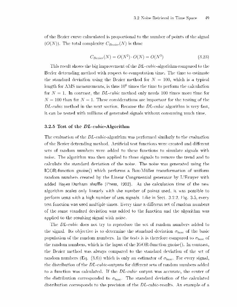
3.2 Noise Retrieval in Time Space 49
of the Bezier curve caluculated is proportional to the number of points of the signal
(O(N)). The total complexity CBezier(N) is thus:
CBezier(N) = O(N2) ·O(N) = O(N3) (3.23)
This result shows the big improvement of theDL-cubic-algorithm compared to the
Bezier detrending method with respect to computation time. The time to estimate
the standard deviation using the Bezier method for N = 100, which is a typical
length for AMS measurements, is thus 106 times the time to perform the calculation
for N = 1. In contrast, the DL-cubic method only needs 100 times more time for
N = 100 than for N = 1. These considerations are important for the testing of the
DL-cubic method in the next section. Because the DL-cubic algorithm is very fast,
it can be tested with millions of generated signals without consuming much time.
3.2.5 Test of the DL-cubic-Algorithm
The evaluation of the DL-cubic-algorithm was performed similarly to the evaluation
of the Bezier detrending method. Arti�cial test functions were created and di�erent
sets of random numbers were added to these functions to simulate signals with
noise. The algorithm was then applied to these signals to remove the trend and to
calculate the standard deviation of the noise. The noise was generated using the
IGOR-function gnoise() which performs a Box-Müller transformation of uniform
random numbers created by the Linear Congruential generator by L'Evuyer with
added Bayes-Durham shu�e (Press, 1992). As the calculation time of the new
algorithm scales only linearly with the number of points used, it was possible to
perform tests with a high number of test signals. Like in Sect. 3.2.2, Fig. 3.5, every
test function was used multiple times. Every time a di�erent set of random numbers
of the same standard deviation was added to the function and the algorithm was
applied to the resulting signal with noise.
The DL-cubic does not try to reproduce the set of random numbers added to
the signal. Its objective is to determine the standard deviation σbase of the basic
population of the random numbers. In the tests it is therefore compared to σbase of
the random numbers, which is the input of the IGOR-function gnoise(). In contrast,
the Bezier method was always compared to the standard deviation of the set of
random numbers (Eq. (3.6)) which is only an estimator of σbase. For every signal,
the distribution of the DL-cubic-outputs for di�erent sets of random numbers added
to a function was calculated. If the DL-cubic output was accurate, the center of
the distribution corresponded to σbase. The standard deviation of the calculated
distribution corresponds to the precision of the DL-cubic-results. An example of a
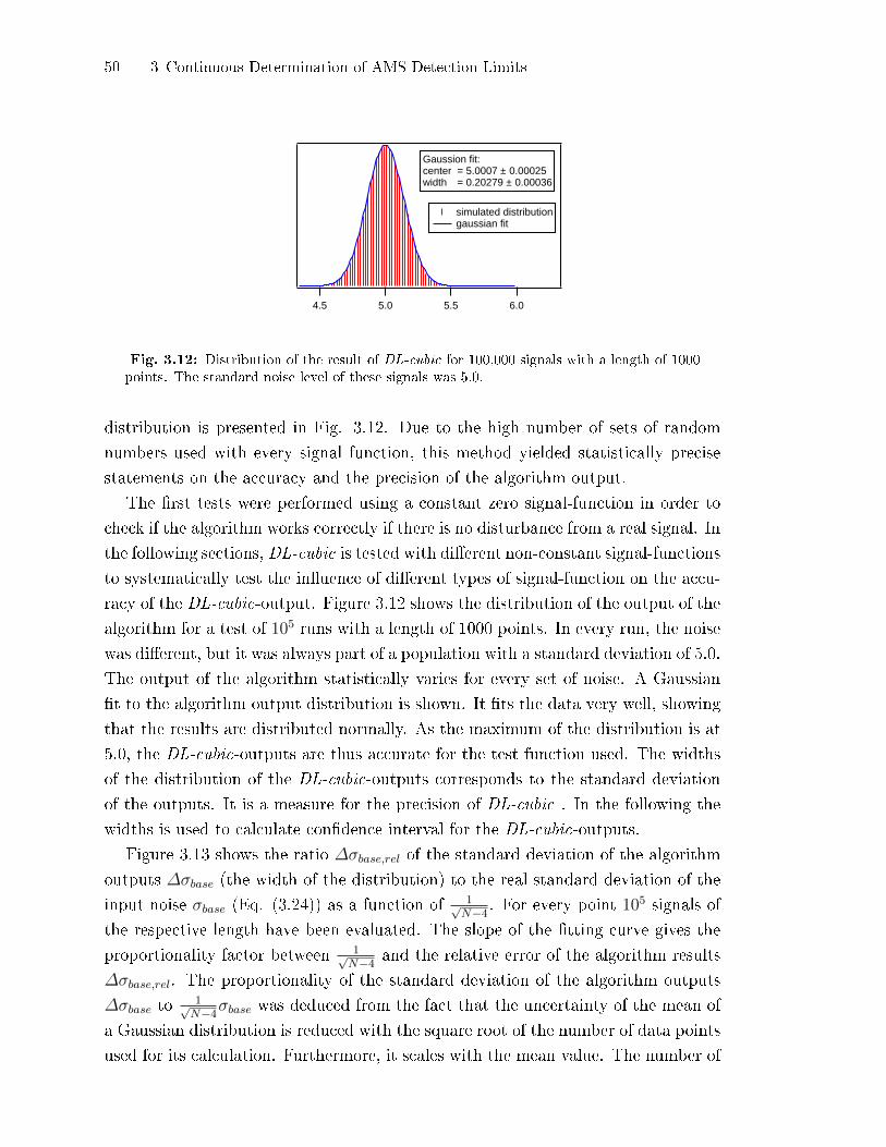
50 3 Continuous Determination of AMS Detection Limits
6.05.55.04.5
Gaussion fit:center = 5.0007 ± 0.00025width = 0.20279 ± 0.00036
simulated distribution gaussian fit
Fig. 3.12: Distribution of the result of DL-cubic for 100,000 signals with a length of 1000points. The standard noise level of these signals was 5.0.
distribution is presented in Fig. 3.12. Due to the high number of sets of random
numbers used with every signal function, this method yielded statistically precise
statements on the accuracy and the precision of the algorithm output.
The �rst tests were performed using a constant zero signal-function in order to
check if the algorithm works correctly if there is no disturbance from a real signal. In
the following sections, DL-cubic is tested with di�erent non-constant signal-functions
to systematically test the in�uence of di�erent types of signal-function on the accu-
racy of the DL-cubic-output. Figure 3.12 shows the distribution of the output of the
algorithm for a test of 105 runs with a length of 1000 points. In every run, the noise
was di�erent, but it was always part of a population with a standard deviation of 5.0.
The output of the algorithm statistically varies for every set of noise. A Gaussian
�t to the algorithm output distribution is shown. It �ts the data very well, showing
that the results are distributed normally. As the maximum of the distribution is at
5.0, the DL-cubic-outputs are thus accurate for the test function used. The widths
of the distribution of the DL-cubic-outputs corresponds to the standard deviation
of the outputs. It is a measure for the precision of DL-cubic . In the following the
widths is used to calculate con�dence interval for the DL-cubic-outputs.
Figure 3.13 shows the ratio ∆σbase,rel of the standard deviation of the algorithm
outputs ∆σbase (the width of the distribution) to the real standard deviation of the
input noise σbase (Eq. (3.24)) as a function of 1√N−4 . For every point 105 signals of
the respective length have been evaluated. The slope of the �tting curve gives the
proportionality factor between 1√N−4 and the relative error of the algorithm results
∆σbase,rel. The proportionality of the standard deviation of the algorithm outputs
∆σbase to1√N−4σbase was deduced from the fact that the uncertainty of the mean of
a Gaussian distribution is reduced with the square root of the number of data points
used for its calculation. Furthermore, it scales with the mean value. The number of
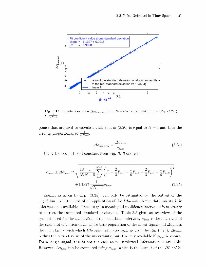
3.2 Noise Retrieval in Time Space 51
4
5
6
789
0.1
2
Ds
base
,rel
4 5 6 7 8 90.1
2
(N-4)-0.5
ratio of the standard deviation of algorithm results to the real standard deviation vs 1/√(N-4)
linear fit
Fit coefficient value ± one standard deviationslope = 1.1327 ± 0.0016R² = 0.9998
Fig. 3.13: Relative deviation ∆σbase,rel of the DL-cubic output distribution (Eq. (3.24))vs. 1√
N−4
points that are used to calculate each sum in (3.20) is equal to N − 4 and thus the
error is proportional to 1√N−4 .
∆σbase,rel =∆σbaseσbase
(3.24)
Using the proportional constant from Fig. 3.13 one gets:
σbase ±∆σbase ∼=
√√√√18
35
1
N − 5
N−3∑i=2
(Fi −
2
3Fi−1 +
1
6Fi−2 −
2
3Fi+1 +
1
6Fi+2
)2
±1.1327 1√N − 4
σbase (3.25)
∆σbase, as given by Eq. (3.25), can only be estimated by the output of the
algorithm, as in the case of an application of the DL-cubic to real data, no statistic
information is available. Thus, to get a meaningful con�dence interval, it is necessary
to correct the estimated standard deviations. Table 3.3 gives an overview of the
symbols used for the calculation of the con�dence intervals. σbase is the real value of
the standard deviation of the noise base population of the input signal and ∆σbase is
the uncertainty with which DL-cubic estimates σbase as given by Eq. (3.25). ∆σbase
is thus the correct value of the uncertainty, but it is only available if σbase is known.
For a single signal, this is not the case as no statistical information is available.
However, ∆σbase can be estimated using σalgo, which is the output of the DL-cubic-

52 3 Continuous Determination of AMS Detection Limits
Table 3.3: Overview of the symbols used to calculate the uncertainty intervals of theDL-cubic-algorithm .
symbol explanation
σbase Standard deviation of the base population of the input noise
∆σbase Real uncertainty in the determination of σalgo,
from the evaluation of a high number of signals
σalgo Estimation of σbase using DL-cubic
∆σalgo Estimation of the uncertainty of σalgo using Eq. (3.25)
algorithm for one signal and thus an estimation of σbase. This yields an estimate of
∆σbase using Eq. (3.25). This estimate is named ∆σalgo.
In case σalgo is an overestimation of σbase, ∆σalgo is also an overestimation of
∆σbase. The other way round, if σalgo is an underestimation,∆σalgo is underestimated
too. The goal of the following consideration is to �nd the correction factor for
∆σalgo as a function of the desired probability that the value of σalgo lies within the
con�dence interval. To do so, two extreme cases were considered: one case with
σalgo being too low by j times ∆σbase and one case with σalgo being to high by j
times ∆σbase. Both cases are summarised in Eq. (3.26).
σbase = σalgo ± j∆σbase (3.26)
∆σ... is proportional to σ...:
∆σbaseσbase
= const. (3.27)
∆σalgoσalgo
= const. (3.28)
As in both equations, Eq. (3.27) and Eq. (3.28), the proportionality constant is
the same, the combination of these equations yields:
∆σbase =σbaseσalgo
∆σalgo
(3.26)=⇒ ∆σbase =
σalgo ± j∆σbaseσalgo
∆σalgo
=∆σalgo ±j∆σbase∆σalgo
σalgo(3.29)
Solving for ∆σbase results in:
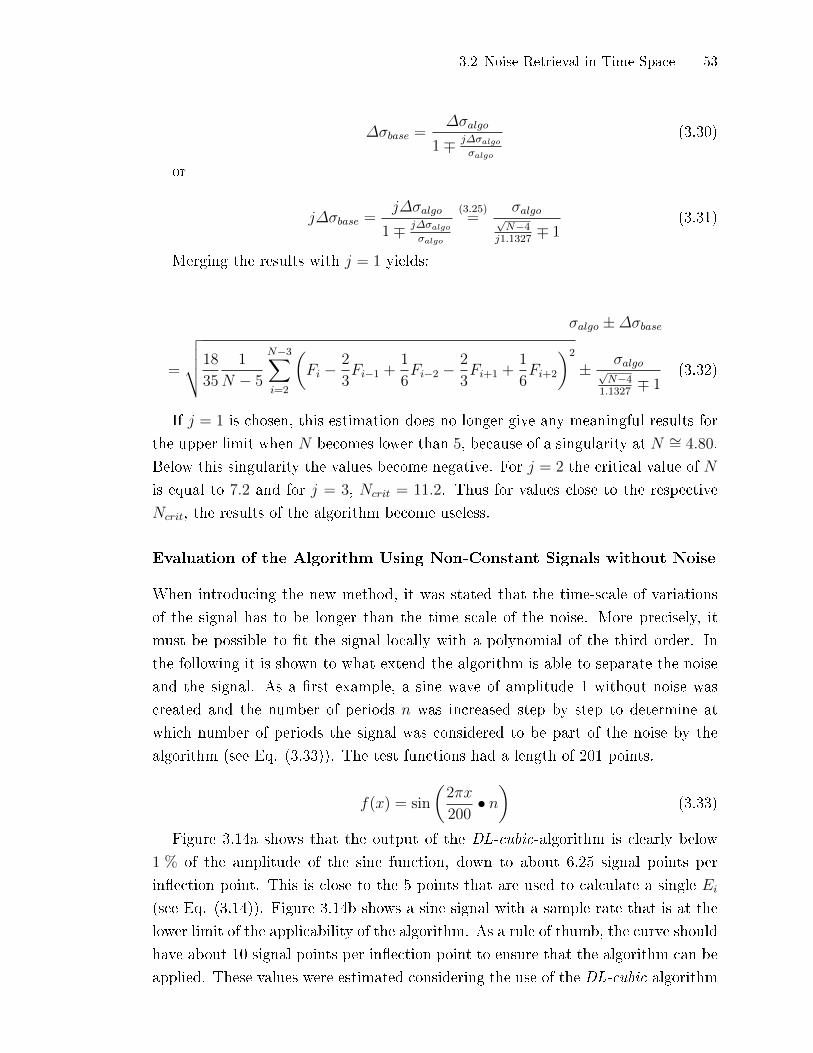
3.2 Noise Retrieval in Time Space 53
∆σbase =∆σalgo
1∓ j∆σalgoσalgo
(3.30)
or
j∆σbase =j∆σalgo
1∓ j∆σalgoσalgo
(3.25)=
σalgo√N−4
j1.1327∓ 1
(3.31)
Merging the results with j = 1 yields:
σalgo ±∆σbase
=
√√√√18
35
1
N − 5
N−3∑i=2
(Fi −
2
3Fi−1 +
1
6Fi−2 −
2
3Fi+1 +
1
6Fi+2
)2
± σalgo√N−4
1.1327∓ 1
(3.32)
If j = 1 is chosen, this estimation does no longer give any meaningful results for
the upper limit when N becomes lower than 5, because of a singularity at N ∼= 4.80.
Below this singularity the values become negative. For j = 2 the critical value of N
is equal to 7.2 and for j = 3, Ncrit = 11.2. Thus for values close to the respective
Ncrit, the results of the algorithm become useless.
Evaluation of the Algorithm Using Non-Constant Signals without Noise
When introducing the new method, it was stated that the time-scale of variations
of the signal has to be longer than the time scale of the noise. More precisely, it
must be possible to �t the signal locally with a polynomial of the third order. In
the following it is shown to what extend the algorithm is able to separate the noise
and the signal. As a �rst example, a sine wave of amplitude 1 without noise was
created and the number of periods n was increased step by step to determine at
which number of periods the signal was considered to be part of the noise by the
algorithm (see Eq. (3.33)). The test functions had a length of 201 points.
f(x) = sin
(2πx
200• n)
(3.33)
Figure 3.14a shows that the output of the DL-cubic-algorithm is clearly below
1 % of the amplitude of the sine function, down to about 6.25 signal points per
in�ection point. This is close to the 5 points that are used to calculate a single Ei
(see Eq. (3.14)). Figure 3.14b shows a sine signal with a sample rate that is at the
lower limit of the applicability of the algorithm. As a rule of thumb, the curve should
have about 10 signal points per in�ection point to ensure that the algorithm can be
applied. These values were estimated considering the use of the DL-cubic algorithm
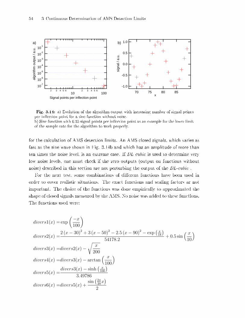
54 3 Continuous Determination of AMS Detection Limits
10-7
10-6
10-5
10-4
10-3
10-2
10-1
algo
rithm
out
put /
a.u
.
2 3 4 5 610
2 3 4 5 6100
Signal points per inflection point
-1.0
-0.5
0.0
0.5
1.0
sign
al /
a.u.
85807570x
a) b)
Fig. 3.14: a) Evolution of the algorithm output with increasing number of signal pointsper in�ection point for a sine function without noise.b) Sine function with 6.25 signal points per in�ection point as an example for the lower limitof the sample rate for the algorithm to work properly.
for the calculation of AMS detection limits. An AMS closed signals, which varies as
fast as the sine wave shown in Fig. 3.14b and which has an amplitude of more than
ten times the noise level, is an extreme case. If DL-cubic is used to determine very
low noise levels, one must check if the zero outputs (output on functions without
noise) described in this section are not perturbing the output of the DL-cubic .
For the next test, some combinations of di�erent functions have been used in
order to cover realistic situations. The exact functions and scaling factors ar not
important. The choice of the functions was done empirically to approximated the
shape of closed signals measured by the AMS. No noise was added to these functions.
The functions used were:
divers1(x) = exp
(−x100
)divers2(x) =
2 (x− 30)2 + 3 (x− 50)2 − 2.5 (x− 90)2 − exp(x18
)54178.2
+ 0.5 sin( x10
)divers3(x) =divers2(x)−
√x
200
divers4(x) =divers3(x)− arctan( x
100
)divers5(x) =
divers3(x)− sinh(x100
)3.49786
divers6(x) =divers5(x) +sin(2π20x)
2
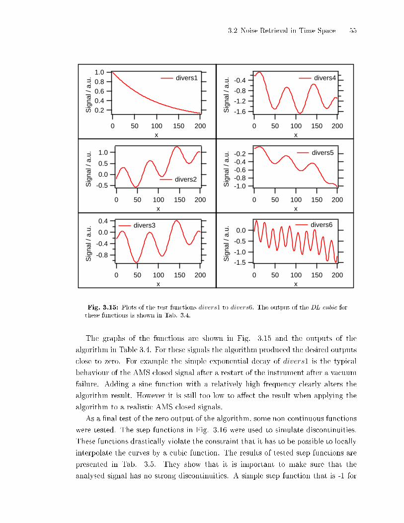
3.2 Noise Retrieval in Time Space 55
1.00.80.60.40.2S
igna
l / a
.u.
200150100500x
divers1
1.0
0.5
0.0
-0.5Sig
nal /
a.u
.
200150100500x
divers2
-0.8
-0.4
0.0
0.4
Sig
nal /
a.u
.
200150100500x
divers3
-1.6
-1.2
-0.8
-0.4
Sig
nal /
a.u
.
200150100500x
divers4
-1.0-0.8-0.6-0.4-0.2
Sig
nal /
a.u
.
200150100500x
divers5
-1.5
-1.0
-0.5
0.0S
igna
l / a
.u.
200150100500x
divers6
Fig. 3.15: Plots of the test functions divers1 to divers6. The output of the DL-cubic forthese functions is shown in Tab. 3.4.
The graphs of the functions are shown in Fig. 3.15 and the outputs of the
algorithm in Table 3.4. For these signals the algorithm produced the desired outputs
close to zero. For example the simple exponential decay of divers1 is the typical
behaviour of the AMS closed signal after a restart of the instrument after a vacuum
failure. Adding a sine function with a relatively high frequency clearly alters the
algorithm result. However it is still too low to a�ect the result when applying the
algorithm to a realistic AMS closed signals.
As a �nal test of the zero output of the algorithm, some non-continuous functions
were tested. The step functions in Fig. 3.16 were used to simulate discontinuities.
These functions drastically violate the constraint that it has to be possible to locally
interpolate the curves by a cubic function. The results of tested step functions are
presented in Tab. 3.5. They show that it is important to make sure that the
analysed signal has no strong discontinuities. A simple step function that is -1 for
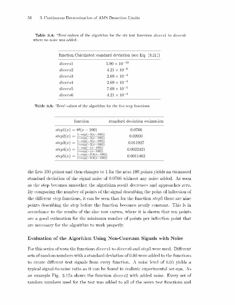
56 3 Continuous Determination of AMS Detection Limits
Table 3.4: �Zero�-values of the algorithm for the six test functions divers1 to divers6where no noise was added.
function Calculated standard deviation (see Eq. (3.21))
divers1 5.90× 10⁻¹⁰
divers2 4.21× 10⁻⁶
divers3 2.69× 10⁻⁴
divers4 2.69× 10⁻⁴
divers5 7.69× 10⁻⁵
divers6 4.21× 10⁻⁴
Table 3.5: �Zero�-values of the algorithm for the �ve step functions
function standard deviation estimation
step1(x) = Θ(x− 100) 0.0766
step2(x) = 1−exp(−3(x−100))1+exp(−3(x−100)) 0.02031
step3(x) = 1−exp(−2(x−100))1+exp(−2(x−100)) 0.011927
step4(x) = 1−exp(−(x−100))1+exp(−(x−100)) 0.0022421
step5(x) = 1−exp(−0.8(x−100))1+exp(−0.8(x−100)) 0.0011462
the �rst 100 points and then changes to 1 for the next 100 points yields an estimated
standard deviation of the signal noise of 0.0766 without any noise added. As soon
as the step becomes smoother the algorithm result decreases and approaches zero.
By comparing the number of points of the signal describing the point of in�ection of
the di�erent step functions, it can be seen that for the function step5 there are nine
points describing the step before the function becomes nearly constant. This is in
accordance to the results of the sine test curves, where it is shown that ten points
are a good estimation for the minimum number of points per in�ection point that
are necessary for the algorithm to work properly.
Evaluation of the Algorithm Using Non-Constant Signals with Noise
For this series of tests the functions divers1 to divers6 and step5 were used. Di�erent
sets of random numbers with a standard deviation of 0.05 were added to the functions
to create di�erent test signals from every function. A noise level of 0.05 yields a
typical signal-to-noise ratio as it can be found in realistic experimental set-ups. As
an example Fig. 3.17a shows the function divers2 with added noise. Every set of
random numbers used for the test was added to all of the seven test functions and

3.2 Noise Retrieval in Time Space 57
-1.0-0.50.00.51.0
Sig
nal /
a.u
.
1041021009896x
step3
-1.0-0.50.00.51.0
Sig
nal /
a.u
.
1041021009896x
step2-1.0-0.50.00.51.0
Sig
nal /
a.u
.
1041021009896x
step5
-1.0-0.50.00.51.0
Sig
nal /
a.u
.
1041021009896x
step4-1.0-0.50.00.51.0
Sig
nal /
a.u
.
1041021009896x
step1
Fig. 3.16: Plots of the test functions step1 to step5
the algorithm was used to retrieve the standard deviation of the random numbers.
This procedure was repeated one million times. Fig. 3.17b shows the histogram of
the results of the algorithm used on the divers2 function with noise. A Gaussian
curve has been �tted to the histogram and the centre of the distribution is 0.050026,
which is in excellent aggrement with the real value of 0.05. The standard deviation
is equal to 0.004 which is equal to the values determined using Eq. (3.21). When
DL-cubic was applied to the other test functions, the distributions of the outputs
had the same centre values and the same relative error as for the divers2 function.
With the new algorithm it is now possible to recalculate the standard deviations
of the test functions used to test the Bezier detrending method. As an example, the
functions considered in Tab. 3.2 are used with the new algorithm. The noise added
to all of these functions had a standard deviation of 0.01. The output of DL-cubic is
summarised in Tab. 3.6. All of the new results are within the 1σ-con�dence interval.
This does not only show the enhanced performance of the new algorithm compared

58 3 Continuous Determination of AMS Detection Limits
1.0
0.5
0.0
-0.5
-1.0
Sig
nal +
noi
se /
a.u.
200150100500x
divers2 + noise
60x10-355504540
algorithm output
mean = 0.050026
a) b)
Fig. 3.17: Function divers2 with noise and a histogram of the results of the algorithmused with this function. The standard deviation of the noise was 0.05.
Table 3.6: Results of the application of the DL-cubic algorithm on the function used totest the Bezier detrending method showed in Tab. 3.2.
function DL-cubic -result up-error down-error
FLAT 0.0087528 0.0017549 0.0012526
SINEXP 0.0090203 0.0018085 0.0012909
SSINEXP 0.0095738 0.0019195 0.0013701
to the Bezier method or any other running mean method but in addition, the results
can be calculated with a con�dence interval which makes them much more reliable.
3.2.6 Detection of Points Not Ful�lling the DL-cubic Prerequisites
Sometimes it is di�cult to judge if a signal ful�ls the the requirement that it can
be locally approximated by a cubic function. Therefore, a test was included in the
DL-cubic procedure to detect outlier of the Ei-values which have been de�ned in
Eq. (3.14). If for a given index i = a, Ea is signi�cantly higher than the average
level of the Ei-values this value can be considered as an outlier and the point Fa
should be excluded from the calculation. As the value of Fa also interferes with
the values of Ea±1 and Ea±2, these values will be lost too for the estimation of the
standard deviation. To detect the outliers, a test described in Barnett and Lewis
(1994) under the name Nµ6 is used. Accordingly this so called discordancy test is
the best test to detect one or more outliers in a normally distributed sample if its
mean value µ is known and the variance σ2 is unknown. In the present case the
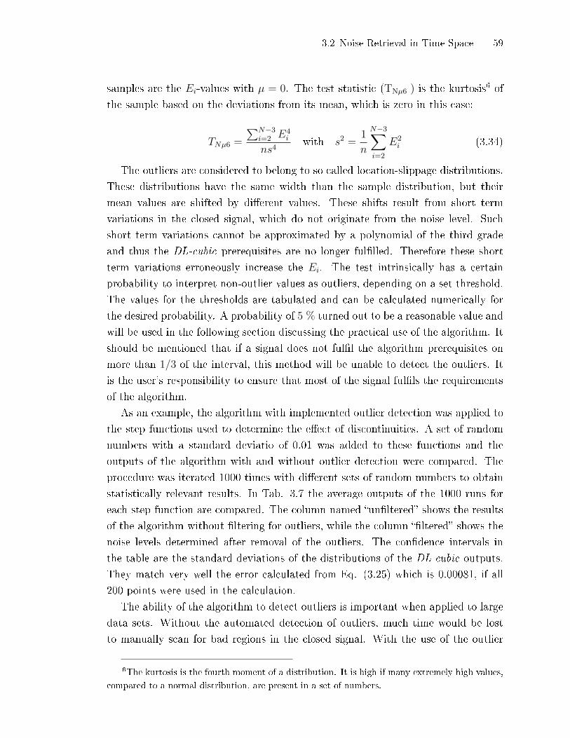
3.2 Noise Retrieval in Time Space 59
samples are the Ei-values with µ = 0. The test statistic (TNµ6 ) is the kurtosis6 of
the sample based on the deviations from its mean, which is zero in this case:
TNµ6 =
∑N−3i=2 E4
i
ns4with s2 =
1
n
N−3∑i=2
E2i (3.34)
The outliers are considered to belong to so called location-slippage distributions.
These distributions have the same width than the sample distribution, but their
mean values are shifted by di�erent values. These shifts result from short term
variations in the closed signal, which do not originate from the noise level. Such
short term variations cannot be approximated by a polynomial of the third grade
and thus the DL-cubic prerequisites are no longer ful�lled. Therefore these short
term variations erroneously increase the Ei. The test intrinsically has a certain
probability to interpret non-outlier values as outliers, depending on a set threshold.
The values for the thresholds are tabulated and can be calculated numerically for
the desired probability. A probability of 5 % turned out to be a reasonable value and
will be used in the following section discussing the practical use of the algorithm. It
should be mentioned that if a signal does not ful�l the algorithm prerequisites on
more than 1/3 of the interval, this method will be unable to detect the outliers. It
is the user's responsibility to ensure that most of the signal ful�ls the requirements
of the algorithm.
As an example, the algorithm with implemented outlier detection was applied to
the step functions used to determine the e�ect of discontinuities. A set of random
numbers with a standard deviatio of 0.01 was added to these functions and the
outputs of the algorithm with and without outlier detection were compared. The
procedure was iterated 1000 times with di�erent sets of random numbers to obtain
statistically relevant results. In Tab. 3.7 the average outputs of the 1000 runs for
each step function are compared. The column named �un�ltered� shows the results
of the algorithm without �ltering for outliers, while the column ��ltered� shows the
noise levels determined after removal of the outliers. The con�dence intervals in
the table are the standard deviations of the distributions of the DL-cubic outputs.
They match very well the error calculated from Eq. (3.25) which is 0.00081, if all
200 points were used in the calculation.
The ability of the algorithm to detect outliers is important when applied to large
data sets. Without the automated detection of outliers, much time would be lost
to manually scan for bad regions in the closed signal. With the use of the outlier
6The kurtosis is the fourth moment of a distribution. It is high if many extremely high values,
compared to a normal distribution, are present in a set of numbers.

60 3 Continuous Determination of AMS Detection Limits
Table 3.7: Comparison of the algorithm outputs for the step functions described in Tab.3.5 without outlier detection (un�ltered) to the results when the �ltering for outliers wasapplied (�ltered). For these tests normal noise with an amplitude of 0.01 was added to thesignal. The table shows the average output for 1000 di�erent noise functions together withthe estimated standard deviations.
function un�ltered �ltered
step1 0.0772±0.0011 0.00991±0.00087step2 0.02262±0.00074 0.00991±0.00088step3 0.01555±0.00071 0.01010±0.00087step4 0.01022±0.00081 0.01012±0.00086step5 0.01004±0.00082 0.00999±0.00085
detection it is su�cient to ensure that the data is not violating the DL-cubic -
prerequisites for more than 1/3 of the signal interval used to determine the noise
level. This can be achieved by a quick investigation of the time series of the signal.
3.2.7 Application to Retrieve AMS Detection Limits
The goal of the development of the DL-cubic-algorithm was to determine AMS
detection limits based on the continuous method introduced by Drewnick et al.
(2009). Drewnick et al. (2009) calculated the detection limits directly from the
closed signal after conversion to mass concentrations. Thus their results already
had the dimension of a mass concentration. However, a closed signal which was
converted to mass concentrations, includes the random variations of the inlet �ow
and the airbeam correction (see Sect. 2.1.9). These additional random variations
are multiplied by the closed signal intensity. If the closed signal is high, the airbeam
correction and the inlet �ow thus introduce large random variations, which are
attributed to the detection limit by the DL-cubic . This is not correct because this
apparent noise is mostly removed in the calculation of the di�erence signal as the
inlet �ow and the airbeam correction are multiplied to both, the closed and the
open signal (see Sec. 2.1). The algorithm must thus be applied directly to the
counts time series prior to the conversion to mass concentrations. This results is a
counts noise level σcnt, which needs to be converted to a mass concentration noise
level σmc using Eq. (2.1). The �ow rate Qin and the airbeam correction factor fAB
are substituted by their respective average values Qin and fAB for the interval the
detection limit is calculated for. This introduces only a very small error as long as
the �ow rate and the airbeam do not drastically change during the period for which
the DL is calculated. This is normally ful�lled. Typically the time periods spent
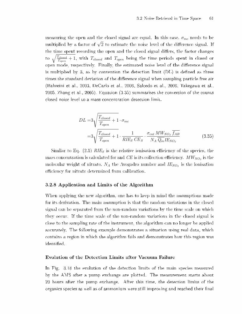
3.2 Noise Retrieval in Time Space 61
measuring the open and the closed signal are equal. In this case, σmc needs to be
multiplied by a factor of√2 to estimate the noise level of the di�erence signal. If
the time spent recording the open and the closed signal di�ers, the factor changes
to√
TclosedTopen
+ 1, with Tclosed and Topen being the time periods spent in closed or
open mode, respectively. Finally, the estimated noise level of the di�erence signal
is multiplied by 3, as by convention the detection limit (DL) is de�ned as three
times the standard deviation of the di�erence signal when sampling particle free air
(Bahreini et al., 2003, DeCarlo et al., 2006, Salcedo et al., 2006, Takegawa et al.,
2005, Zhang et al., 2005). Equation (3.35) summarises the conversion of the counts
closed noise level to a mass concentration detection limit.
DL =3
√TclosedTopen
+ 1 ·σmc
=3
√TclosedTopen
+ 1 · 1
RIES CES
· σcnt MWNO3 fAB
NA QinIENO3
(3.35)
Similar to Eq. (2.1) RIES is the relative ionisation e�ciency of the species, the
mass concentration is calculated for and CE is its collection e�ciency. MWNO3 is the
molecular weight of nitrate, NA the Avogadro number and IENO3 is the ionisation
e�ciency for nitrate determined from calibration.
3.2.8 Application and Limits of the Algorithm
When applying the new algorithm, one has to keep in mind the assumptions made
for its derivation. The main assumption is that the random variations in the closed
signal can be separated from the non-random variations by the time scale on which
they occur. If the time scale of the non-random variations in the closed signal is
close to the sampling rate of the instrument, the algorithm can no longer be applied
accurately. The following example demonstrates a situation using real data, which
contains a region in which the algorithm fails and demonstrates how this region was
identi�ed.
Evolution of the Detection Limits after Vacuum Failure
In Fig. 3.18 the evolution of the detection limits of the main species measured
by the AMS after a pump exchange are plotted. The measurement starts about
20 hours after the pump exchange. After this time, the detection limits of the
organics species as well as of ammonium were still improving and reached their �nal
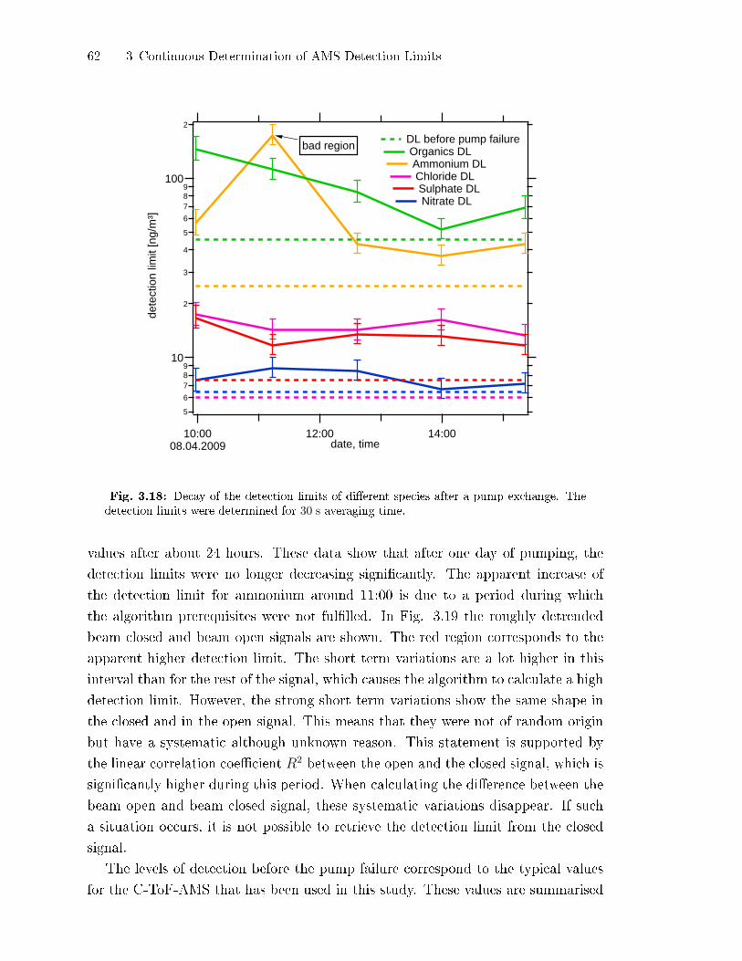
62 3 Continuous Determination of AMS Detection Limits
5
6
789
10
2
3
4
5
6
789
100
2
dete
ctio
n lim
it [n
g/m
³]
10:0008.04.2009
12:00 14:00date, time
DL before pump failure Organics DL Ammonium DL Chloride DL Sulphate DL Nitrate DL
bad region
Fig. 3.18: Decay of the detection limits of di�erent species after a pump exchange. Thedetection limits were determined for 30 s averaging time.
values after about 24 hours. These data show that after one day of pumping, the
detection limits were no longer decreasing signi�cantly. The apparent increase of
the detection limit for ammonium around 11:00 is due to a period during which
the algorithm prerequisites were not ful�lled. In Fig. 3.19 the roughly detrended
beam closed and beam open signals are shown. The red region corresponds to the
apparent higher detection limit. The short term variations are a lot higher in this
interval than for the rest of the signal, which causes the algorithm to calculate a high
detection limit. However, the strong short term variations show the same shape in
the closed and in the open signal. This means that they were not of random origin
but have a systematic although unknown reason. This statement is supported by
the linear correlation coe�cient R2 between the open and the closed signal, which is
signi�cantly higher during this period. When calculating the di�erence between the
beam open and beam closed signal, these systematic variations disappear. If such
a situation occurs, it is not possible to retrieve the detection limit from the closed
signal.
The levels of detection before the pump failure correspond to the typical values
for the C-ToF-AMS that has been used in this study. These values are summarised
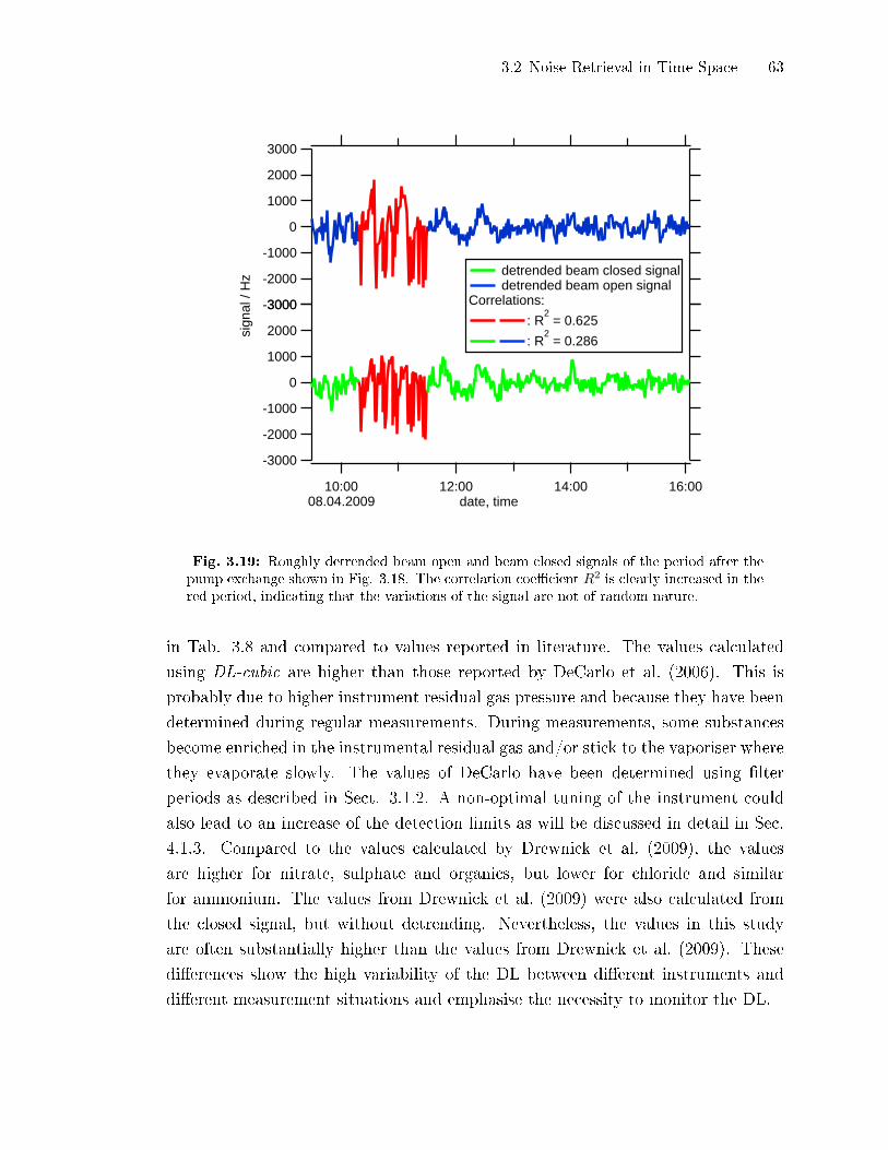
3.2 Noise Retrieval in Time Space 63
-3000
-2000
-1000
0
1000
2000
3000
sign
al /
Hz
10:0008.04.2009
12:00 14:00 16:00date, time
-3000
-2000
-1000
0
1000
2000
3000
detrended beam closed signal detrended beam open signal
Correlations:
: R2 = 0.625
: R2 = 0.286
Fig. 3.19: Roughly detrended beam open and beam closed signals of the period after thepump exchange shown in Fig. 3.18. The correlation coe�cient R2 is clearly increased in thered period, indicating that the variations of the signal are not of random nature.
in Tab. 3.8 and compared to values reported in literature. The values calculated
using DL-cubic are higher than those reported by DeCarlo et al. (2006). This is
probably due to higher instrument residual gas pressure and because they have been
determined during regular measurements. During measurements, some substances
become enriched in the instrumental residual gas and/or stick to the vaporiser where
they evaporate slowly. The values of DeCarlo have been determined using �lter
periods as described in Sect. 3.1.2. A non-optimal tuning of the instrument could
also lead to an increase of the detection limits as will be discussed in detail in Sec.
4.1.3. Compared to the values calculated by Drewnick et al. (2009), the values
are higher for nitrate, sulphate and organics, but lower for chloride and similar
for ammonium. The values from Drewnick et al. (2009) were also calculated from
the closed signal, but without detrending. Nevertheless, the values in this study
are often substantially higher than the values from Drewnick et al. (2009). These
di�erences show the high variability of the DL between di�erent instruments and
di�erent measurement situations and emphasise the necessity to monitor the DL.
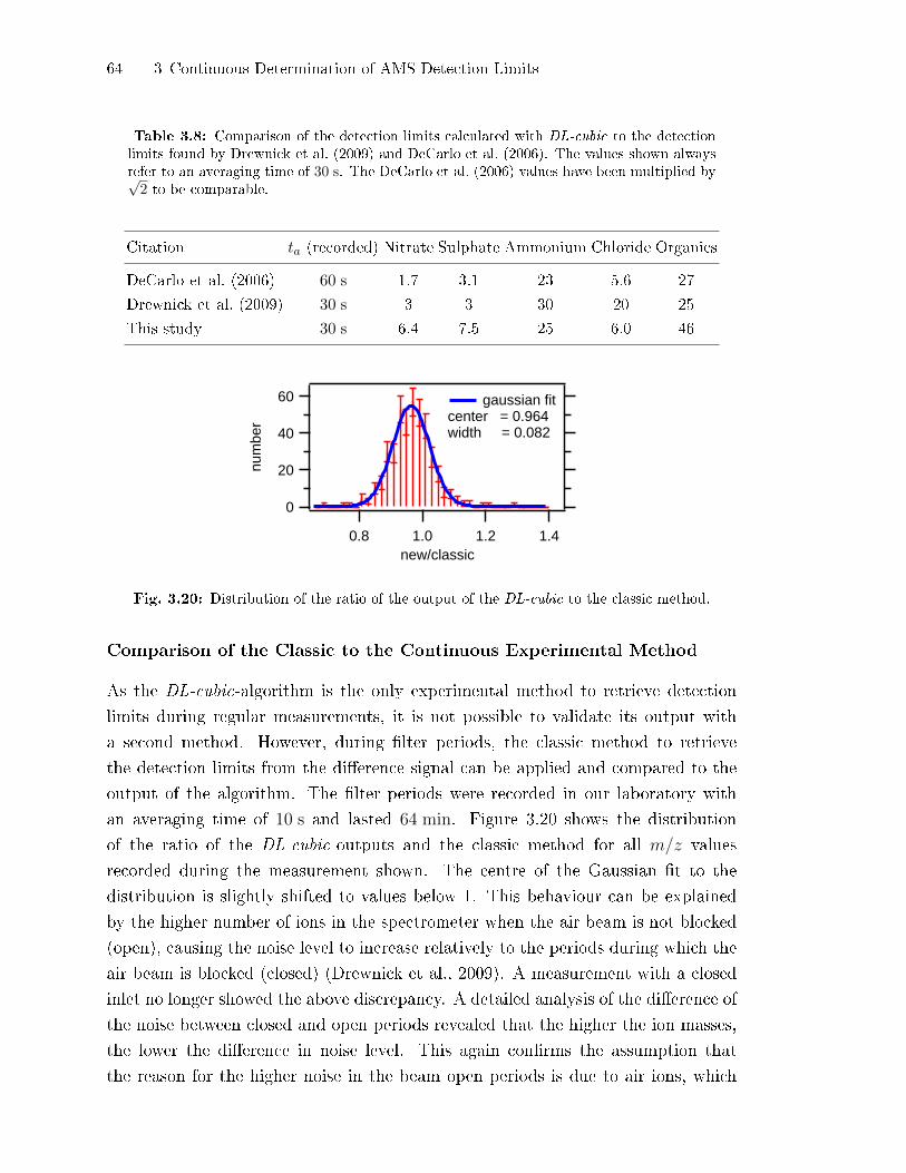
64 3 Continuous Determination of AMS Detection Limits
Table 3.8: Comparison of the detection limits calculated with DL-cubic to the detectionlimits found by Drewnick et al. (2009) and DeCarlo et al. (2006). The values shown alwaysrefer to an averaging time of 30 s. The DeCarlo et al. (2006) values have been multiplied by√2 to be comparable.
Citation ta (recorded) Nitrate Sulphate Ammonium Chloride Organics
DeCarlo et al. (2006) 60 s 1.7 3.1 23 5.6 27
Drewnick et al. (2009) 30 s 3 3 30 20 25
This study 30 s 6.4 7.5 25 6.0 46
60
40
20
0
num
ber
1.41.21.00.8new/classic
gaussian fitcenter = 0.964width = 0.082
Fig. 3.20: Distribution of the ratio of the output of the DL-cubic to the classic method.
Comparison of the Classic to the Continuous Experimental Method
As the DL-cubic-algorithm is the only experimental method to retrieve detection
limits during regular measurements, it is not possible to validate its output with
a second method. However, during �lter periods, the classic method to retrieve
the detection limits from the di�erence signal can be applied and compared to the
output of the algorithm. The �lter periods were recorded in our laboratory with
an averaging time of 10 s and lasted 64 min. Figure 3.20 shows the distribution
of the ratio of the DL-cubic-outputs and the classic method for all m/z values
recorded during the measurement shown. The centre of the Gaussian �t to the
distribution is slightly shifted to values below 1. This behaviour can be explained
by the higher number of ions in the spectrometer when the air beam is not blocked
(open), causing the noise level to increase relatively to the periods during which the
air beam is blocked (closed) (Drewnick et al., 2009). A measurement with a closed
inlet no longer showed the above discrepancy. A detailed analysis of the di�erence of
the noise between closed and open periods revealed that the higher the ion masses,
the lower the di�erence in noise level. This again con�rms the assumption that
the reason for the higher noise in the beam open periods is due to air ions, which
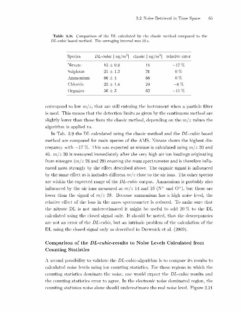
3.2 Noise Retrieval in Time Space 65
Table 3.9: Comparison of the DL calculated by the classic method compared to theDL-cubic based method. The averaging interval was 10 s.
Species DL-cubic [ ng/m3] classic [ ng/m3] relative error
Nitrate
Sulphate
Ammonium
Chloride
Organics
15 ± 0.9
21 ± 1.3
66 ± 4
22 ± 1.4
56 ± 3
18
21
66
24
62
−17 %
0 %
0 %
−6 %
−11 %
correspond to low m/z, that are still entering the instrument when a particle �lter
is used. This means that the detection limits as given by the continuous method are
slightly lower than those from the classic method, depending on the m/z values the
algorithm is applied to.
In Tab. 3.9 the DL calculated using the classic method and the DL-cubic based
method are compared for main species of the AMS. Nitrate shows the highest dis-
crepancy with −17 %. This was expected as nitrate is calculated using m/z 30 and
46. m/z 30 is measured immediately after the very high air ion loadings originating
from nitrogen (m/z 28 and 29) entering the mass spectrometer and is therefore in�u-
enced most strongly by the e�ect described above. The organic signal is in�uenced
by the same e�ect as it includes di�erentm/z close to the air ions. The other species
are within the expected range of the DL-cubic output. Ammonium is probably also
in�uenced by the air ions measured at m/z 14 and 16 (N+ and O+), but these are
lower than the signal of m/z 28. Because ammonium has a high noise level, the
relative e�ect of the ions in the mass spectrometer is reduced. To make sure that
the nitrate DL is not underestimated it might be useful to add 20 % to the DL
calculated using the closed signal only. It should be noted, that the descrepancies
are not an error of the DL-cubic, but an intrinsic problem of the calculation of the
DL using the closed signal only as described in Drewnick et al. (2009).
Comparison of the DL-cubic-results to Noise Levels Calculated from
Counting Statistics
A second possibility to validate the DL-cubic-algorithm is to compare its results to
calculated noise levels using ion counting statistics. For those regions in which the
counting statistics dominate the noise, one would expect the DL-cubic results and
the counting statistics error to agree. In the electronic noise dominated region, the
counting statistics noise alone should underestimate the real noise level. Figure 3.21

66 3 Continuous Determination of AMS Detection Limits
102
103
104
105
DL_
cubi
c no
ise
leve
l / c
ount
s
101
102
103
104
counting statistics noise level / counts
Counting statisticsdominated region
electronic noisedominated region
DL_cubic results fit with signal independent noise (∆I)
Fig. 3.21: Comparison of the results of the continuous method to the counting statistics.The noise level was estimated for every m/z using the new method and by calculatingcounting statistics. The data was �tted using Eq. (3.36).
shows the comparison of the output of the DL-cubic-tool to the noise level calculated
from counting statistics alone (red dots). The data was recorded during the labo-
ratory measurement campaign ACI-03 at the AIDA facility. The counting statistics
noise level was calculated from the output of the evaluation tool SQUIRREL (Sect.
2.1.10) and summed for a whole day. As the signal of a single ion event (Sect. 2.1.6)
is varying from ion to ion, the counting statistic distribution is convoluted with the
distribution of a single ion signal. Therefore the width of the counts distribution is
increased by a factor σ = 1.2. The counts from SQUIRREL included the correction
of the overshooting duty cycle (Sect. 2.1.7). This correction could not be undone,
as the necessary parameters were not accessible. Due to all these factors, no one to
one relation can be expected in Fig. 3.21, even in the counting statistics dominated
region with high signal.
To be able to compare the experimental noise level with the noise level estimated
from the counting statistics, a model accounting for random noise α was �tted to
the data using Eq. (3.36) (blue points in Fig. 3.21):

3.2 Noise Retrieval in Time Space 67
∆I =
√TintFpulstmeas
VSI
(Aduty)2
m/zα2 + σI
Aduty√m/z
(3.36)
I is the counts signal as given by SQUIRREL and ∆I is the modelled noise level.
Tint is the time integrating the signal which is attributed to onem/z during one pulse
of the mass spectrometer. Fpuls is the number of pulses of the mass spectrometer per
second and tmeas is the total time spend measuring. T = Tint × Fpuls × tmeas is thusthe time spend averaging one m/z during the measurement. VSI is a unit conversion
factor equal to the area below a single ion signal. All these values are accessible in
SQUIRREL.Aduty is a �tting parameter scaling the duty cycle correction e�ect which
is proportional to√m/z (Sect. 2.1.7). This parameter was �tted as the value used
by SQUIRREL was not accessible. It was also not possible to calculate the value
as the exact quantities necessary could not be accessed. The �t using this model
function looks �ne, but a more detailed analysis reveals some weaknesses. Both, the
DL-cubic-results and the �t seem to have a high noise level. However, the apparent
random variations of the curve are not only due to noise. Part of them are due to the
duty cycle correction. The duty cycle correction continuously varies with√m/z.
As the signal corresponding to the di�erent m/z is spread over the whole signal
intensity range, the duty cycle correction is varying between neighbouring points.
These variations appear to be a random variation although they are systematic. To
optically improve the comparison between the �t and the experimental values, the
noise level determined by the �tted model function can be directly plotted versus the
DL-cubic-outputs. The data should now be situated on the one-to-one-line. This
graph is presented in Fig. 3.22. It shows that the model function overestimates the
noise when the DL-cubic-output is high and very low. Furthermore, the noise is
systematically underestimated when it is between 200 and 1000 counts. To account
for this e�ect, the source of the random noise needs to be examined in detail.
Analysis of the recording of noise in the AMS
To improve the AMS signal to noise ratio, only signals that exceed a certain thresh-
old value are recorded (Sect. 2.1.4). This produces a term, which is up to now not
considered in the AMS standard evaluation procedures and which is signal depen-
dent. It is mathematically deduced in the following.
Figure 3.23 shows the e�ect of thresholding on the recorded noise. In the upper
panel pure noise is shown and in the middle panel this noise was added to a signal.
This signal is now subject to thresholding with a threshold of 4. Only those points
with the signal above the threshold are recorded and thus only the noise coinciding
with these points above the threshold is recorded. The noise which passes the
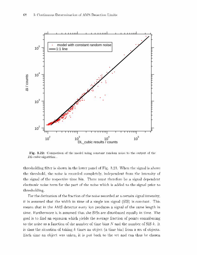
68 3 Continuous Determination of AMS Detection Limits
102
103
104
105
∆I /
coun
ts
102
103
104
105
DL_cubic results / counts
model with constant random noise1:1 line
Fig. 3.22: Comparison of the model using constant random noise to the output of theDL-cubic-algorithm .
thresholding �lter is shown in the lower panel of Fig. 3.23. When the signal is above
the threshold, the noise is recorded completely, independent from the intensity of
the signal of the respective time bin. There must therefore be a signal dependent
electronic noise term for the part of the noise which is added to the signal prior to
thresholding.
For the derivation of the fraction of the noise recorded at a certain signal intensity,
it is assumed that the width in time of a single ion signal (SIS) is constant. This
means that in the AMS detector every ion produces a signal of the same length in
time. Furthermore it is assumed that the SISs are distributed equally in time. The
goal is to �nd an equation which yields the average fraction of points contributing
to the noise as a function of the number of time bins N and the number of SIS k. It
is thus the situation of taking k times an object (a time bin) from a set of objects.
Each time an object was taken, it is put back to the set and can thus be chosen
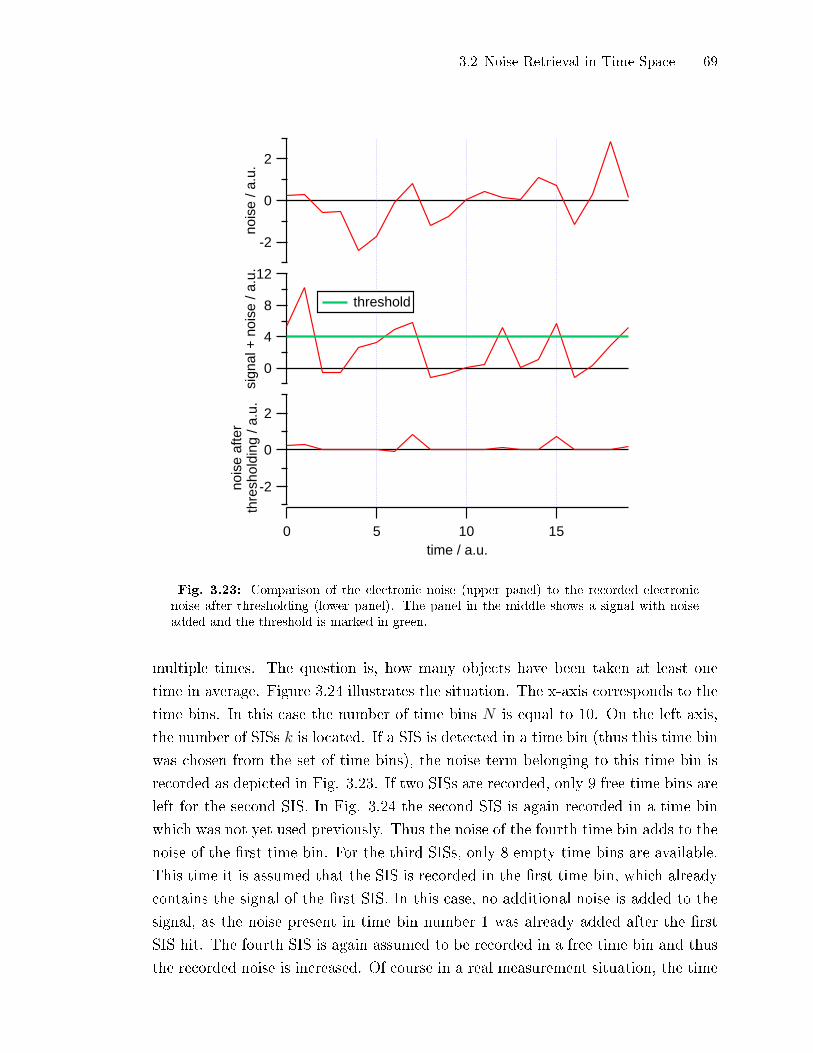
3.2 Noise Retrieval in Time Space 69
-2
0
2
nois
e / a
.u.
151050time / a.u.
12
8
4
0
sign
al +
noi
se /
a.u.
-2
0
2
nois
e af
ter
thre
shol
ding
/ a.
u.
threshold
Fig. 3.23: Comparison of the electronic noise (upper panel) to the recorded electronicnoise after thresholding (lower panel). The panel in the middle shows a signal with noiseadded and the threshold is marked in green.
multiple times. The question is, how many objects have been taken at least one
time in average. Figure 3.24 illustrates the situation. The x-axis corresponds to the
time bins. In this case the number of time bins N is equal to 10. On the left axis,
the number of SISs k is located. If a SIS is detected in a time bin (thus this time bin
was chosen from the set of time bins), the noise term belonging to this time bin is
recorded as depicted in Fig. 3.23. If two SISs are recorded, only 9 free time bins are
left for the second SIS. In Fig. 3.24 the second SIS is again recorded in a time bin
which was not yet used previously. Thus the noise of the fourth time bin adds to the
noise of the �rst time bin. For the third SISs, only 8 empty time bins are available.
This time it is assumed that the SIS is recorded in the �rst time bin, which already
contains the signal of the �rst SIS. In this case, no additional noise is added to the
signal, as the noise present in time bin number 1 was already added after the �rst
SIS hit. The fourth SIS is again assumed to be recorded in a free time bin and thus
the recorded noise is increased. Of course in a real measurement situation, the time
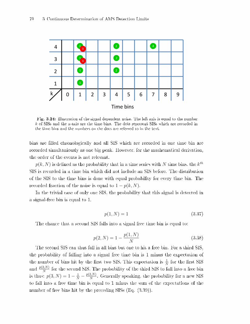
70 3 Continuous Determination of AMS Detection Limits
Time bins
0 1 2 3 4 5 6 7 8 9
1
2
3
4
k
1
1 2
1 2 3
1 3
4 2
Fig. 3.24: Illustration of the signal dependent noise. The left axis is equal to the numberk of SISs and the x-axis are the time bins. The dots represent SISs which are recorded inthe time bins and the numbers on the dots are referred to in the text.
bins are �lled chronologically and all SIS which are recorded in one time bin are
recorded simultaniously as one big peak. However, for the mathematical derivation,
the order of the events is not relevant.
p(k,N) is de�ned as the probability that in a time series with N time bins, the kth
SIS is recorded in a time bin which did not include an SIS before. The distribution
of the SIS to the time bins is done with equal probability for every time bin. The
recorded fraction of the noise is equal to 1− p(k,N).
In the trivial case of only one SIS, the probability that this signal is detected in
a signal-free bin is equal to 1.
p(1, N) = 1 (3.37)
The chance that a second SIS falls into a signal free time bin is equal to:
p(2, N) = 1− p(1, N)
N(3.38)
The second SIS can thus fall in all bins but one to hit a free bin. For a third SIS,
the probability of falling into a signal free time bin is 1 minus the expectation of
the number of bins hit by the �rst two SIS. This expectation is 1Nfor the �rst SIS
and p(2,N)N
for the second SIS. The probability of the third SIS to fall into a free bin
is thus: p(3, N) = 1− 1N− p(2,N)
N. Generally speaking, the probability for a new SIS
to fall into a free time bin is equal to 1 minus the sum of the expectations of the
number of free bins hit by the preceding SISs (Eq. (3.39)).
3.2 Noise Retrieval in Time Space 71
p(k,N) = 1−k−1∑i=1
p(i, N)
N(3.39)
The calculation of p(k,N) de�ned recursively is very expensive with respect to
computation time. It is thus preferable to have an explicit form of p(k,N). The
explicit form of p(k,N) is:
p(k,N) =
(1− 1
N
)k−1(3.40)
This can be proven by mathematical induction.
Base case:
p(1, N) =
(1− 1
N
)1−1
= 1 (3.41)
The proposed equation is thus true for the base case. The inductive hypothesis
is given by Eq. (3.40) and the inductive step is:
p(k + 1, N) = 1−k−1∑i=1
p(i, N)
N(3.42)
= 1−∑k
i=1 p(i, N)
N(3.43)
= 1−∑k−1
i=1 p(i, N) + p(k,N)
N(3.44)
= 1−∑k−1
i=1 p(i, N)
N− p(k,N)
N(3.45)
= p(k,N)− p(k,N)
N(3.46)
=
(1− 1
N
)k−1−(1− 1
N
)k−1N
by Eq. (3.40) (3.47)
=
(1− 1
N
)k−1(1− 1
N
)(3.48)
=
(1− 1
N
)kq.e.d. (3.49)
It has been proven that if the assumed explicit form of p(k,N) is correct for k
SIS, it is also correct for k + 1 SIS. This means that if it was correct for k = 1, it is
also correct for k = 2. This also means that it must be correct for k = 3 and so on.
With this new term, the equation describing the noise ∆I of the AMS reads:
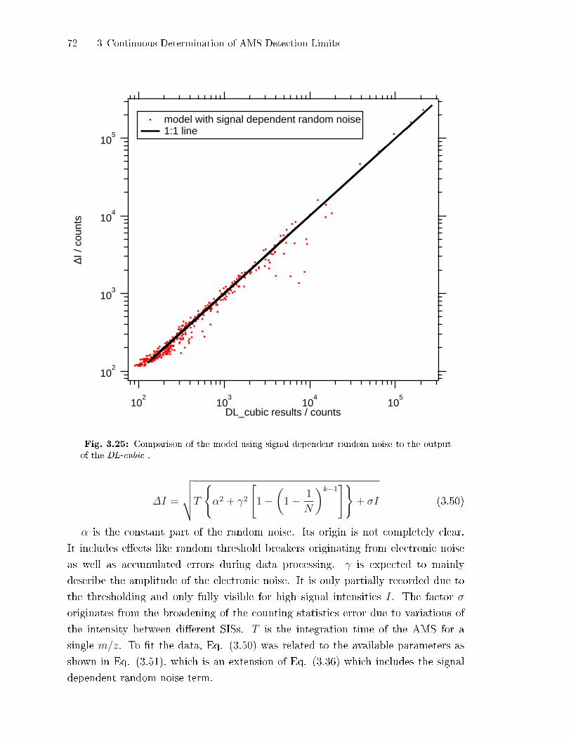
72 3 Continuous Determination of AMS Detection Limits
102
103
104
105
∆I /
coun
ts
102
103
104
105
DL_cubic results / counts
model with signal dependent random noise 1:1 line
Fig. 3.25: Comparison of the model using signal dependent random noise to the outputof the DL-cubic .
∆I =
√√√√T
{α2 + γ2
[1−
(1− 1
N
)k−1]}+ σI (3.50)
α is the constant part of the random noise. Its origin is not completely clear.
It includes e�ects like random threshold breakers originating from electronic noise
as well as accumulated errors during data processing. γ is expected to mainly
describe the amplitude of the electronic noise. It is only partially recorded due to
the thresholding and only fully visible for high signal intensities I. The factor σ
originates from the broadening of the counting statistics error due to variations of
the intensity between di�erent SISs. T is the integration time of the AMS for a
single m/z. To �t the data, Eq. (3.50) was related to the available parameters as
shown in Eq. (3.51), which is an extension of Eq. (3.36) which includes the signal
dependent random noise term.

3.2 Noise Retrieval in Time Space 73
Table 3.10: Overview of the parameters in the �tting equation (3.51)
Parameter Description �tted?
α constant random noise yes
γ signal dependent random noise yes
Tint time integrated for one m/z per spectra no
Fpuls number of spectra recorded per second no
tmeas number of seconds averaged no
VSI area of a single ion signal no
m/z mass to charge ratio no
S scaling factor for the signal dependent noise term. See text. yes
Aduty factor for the duty cycle correction. See text. yes
∆I =
√√√√√TintFpulstmeasVSI
(Aduty)2
m/z
α2 + γ2
1−(1− 1
tmeasFpulsS
)(IAduty√
m/z−1
)+σI
Aduty√m/z
(3.51)
Figure 3.25 shows the comparison of the new model function to the DL-cubic
data. The discrepancies have nearly completely vanished. Only for very low noise
levels, the model seems to overpredict the noise. Nevertheless, some distinct points
are underestimated close to one order of magnitude. The parameters in Eq. (3.51)
are summarized in Tab. 3.10. The parameters S and Aduty were used as additional
�tting parameters as their values were not accessible. Aduty is the factor of the duty
cycle correction. Its theoretical value is 38.7, calculated using equation (3.12) of
Hings (2007):
Aduty =
(xpulserFpuls
√1
2Uion
1
9824 kgCu eV
)−1(3.52)
with the open length of the pulser electrode xpulser = 46 mm (Drewnick et al., 2005),
Fpuls = 50 kHz, and the voltage in the ion chamber Uion = 41 V. Except for xpulser
the values were retrieved from the recorded AMS data �les. The exact values used
by SQUIRREL were unknown. The �t using Eq. (3.51) yielded a value of 44.2 when
σ was set to 1.2, which is an experimental value described in Allan (2010). When
setting Aduty to 38.7, σ is found to be 1.39. The values found are thus reasonably
close to the theoretical value and the value from literature, respectively. A summary
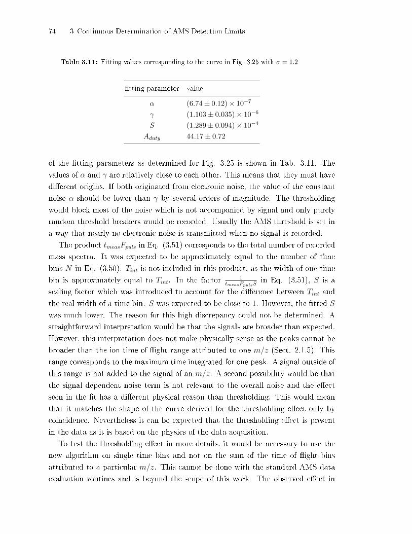
74 3 Continuous Determination of AMS Detection Limits
Table 3.11: Fitting values corresponding to the curve in Fig. 3.25 with σ = 1.2
�tting parameter value
α (6.74± 0.12)× 10−7
γ (1.103± 0.035)× 10−6
S (1.289± 0.094)× 10−4
Aduty 44.17± 0.72
of the �tting parameters as determined for Fig. 3.25 is shown in Tab. 3.11. The
values of α and γ are relatively close to each other. This means that they must have
di�erent origins. If both originated from electronic noise, the value of the constant
noise α should be lower than γ by several orders of magnitude. The thresholding
would block most of the noise which is not accompanied by signal and only purely
random threshold breakers would be recorded. Usually the AMS threshold is set in
a way that nearly no electronic noise is transmitted when no signal is recorded.
The product tmeasFpuls in Eq. (3.51) corresponds to the total number of recorded
mass spectra. It was expected to be approximately equal to the number of time
bins N in Eq. (3.50). Tint is not included in this product, as the width of one time
bin is approximately equal to Tint. In the factor 1tmeasFpulsS
in Eq. (3.51), S is a
scaling factor which was introduced to account for the di�erence between Tint and
the real width of a time bin. S was expected to be close to 1. However, the �tted S
was much lower. The reason for this high discrepancy could not be determined. A
straightforward interpretation would be that the signals are broader than expected.
However, this interpretation does not make physically sense as the peaks cannot be
broader than the ion time of �ight range attributed to one m/z (Sect. 2.1.5). This
range corresponds to the maximum time integrated for one peak. A signal outside of
this range is not added to the signal of an m/z. A second possibility would be that
the signal dependent noise term is not relevant to the overall noise and the e�ect
seen in the �t has a di�erent physical reason than thresholding. This would mean
that it matches the shape of the curve derived for the thresholding e�ect only by
coincidence. Nevertheless it can be expected that the thresholding e�ect is present
in the data as it is based on the physics of the data acquisition.
To test the thresholding e�ect in more details, it would be necessary to use the
new algorithm on single time bins and not on the sum of the time of �ight bins
attributed to a particular m/z. This cannot be done with the standard AMS data
evaluation routines and is beyond the scope of this work. The observed e�ect in
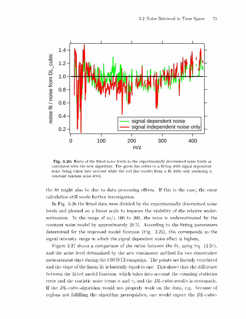
3.2 Noise Retrieval in Time Space 75
1.4
1.2
1.0
0.8
0.6
0.4
0.2
nois
e fit
/ no
ise
from
DL_
cubi
c
4003002001000m/z
signal dependent noise signal independent noise only
Fig. 3.26: Ratio of the �tted noise levels to the experimentally determined noise levels ascalculated with the new algorithm. The green line refers to a �tting with signal dependentnoise being taken into account while the red line results from a �t with only assuming aconstant random noise level.
the �t might also be due to data processing e�ects. If this is the case, the error
calculation still needs further investigation.
In Fig. 3.26 the �tted data were divided by the experimentally determined noise
levels and plotted on a linear scale to improve the visibility of the relative under-
estimation. In the range of m/z 100 to 200, the noise is underestimated by the
constant noise model by approximately 20 %. According to the �tting parameters
determined for the improved model function (Fig. 3.25), this corresponds to the
signal intensity range in which the signal dependent noise e�ect is highest.
Figure 3.27 shows a comparison of the ratios between the �t, using Eq. (3.51),
and the noise level determined by the new continuous method for two consecutive
measurement days during the FROST2 campaign. The points are linearly correlated
and the slope of the linear �t is basically equal to one. This shows that the di�erence
between the �tted model function, which takes into account the counting statistics
error and the statistic noise terms α and γ, and the DL-cubic-results is systematic.
If the DL-cubic-algorithm would not properly work on the data, e.g. because of
regions not ful�lling the algorithm prerequisites, one would expect the DL-cubic-
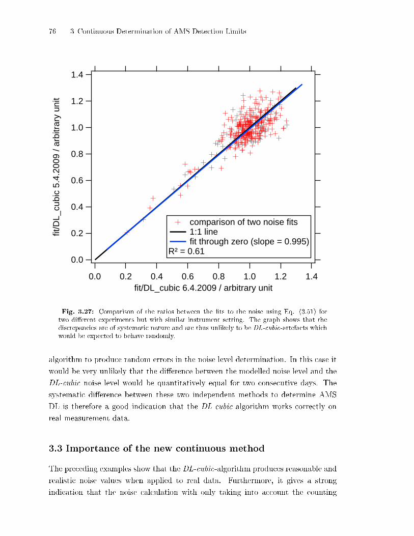
76 3 Continuous Determination of AMS Detection Limits
1.4
1.2
1.0
0.8
0.6
0.4
0.2
0.0
fit/D
L_cu
bic
5.4.
2009
/ ar
bitr
ary
unit
1.41.21.00.80.60.40.20.0fit/DL_cubic 6.4.2009 / arbitrary unit
comparison of two noise fits 1:1 line fit through zero (slope = 0.995)
R² = 0.61
Fig. 3.27: Comparison of the ratios between the �ts to the noise using Eq. (3.51) fortwo di�erent experiments but with similar instrument setting. The graph shows that thediscrepancies are of systematic nature and are thus unlikely to be DL-cubic-artefacts whichwould be expected to behave randomly.
algorithm to produce random errors in the noise level determination. In this case it
would be very unlikely that the di�erence between the modelled noise level and the
DL-cubic noise level would be quantitatively equal for two consecutive days. The
systematic di�erence between these two independent methods to determine AMS
DL is therefore a good indication that the DL-cubic-algorithm works correctly on
real measurement data.
3.3 Importance of the new continuous method
The preceding examples show that the DL-cubic-algorithm produces reasonable and
realistic noise values when applied to real data. Furthermore, it gives a strong
indication that the noise calculation with only taking into account the counting
3.3 Importance of the new continuous method 77
statistics and a constant random noise term is missing part of the noise. Especially
in the transition region from noise to counting statistics dominated signal, this is
likely to cause signi�cant errors. As the detection limits are directly proportional to
the noise levels, the detection limits are underestimated when calculated using the
the model function presented in the preceding section. In the case of low m/z, the
algorithm often determines a noise level that is markedly higher than the calculated
noise level from the counting statistics model. The m/z in this region, which have
low signal intensities, are likely to have much higher DL than the calculated values
using the model function would suggest. The DL are not important for some m/z
in this region as their di�erence signals are very high. However, their errors are
greatly underestimated if only the counting statistics and a random noise term are
considered.
The reasons for these e�ects are not completely clear. There might be physical
reasons in the data acquisition that cause additional noise. However it is likely,
that some of the e�ects are caused by the data evaluation procedures implemented
in SQUIRREL (see Sect. 2.1.10). These e�ects are automatically considered when
applying the DL-cubic-algorithm to determine the detection limits and errors for the
AMS results. As the data evaluation involves many user set parameters which are
not handled uniformly in the user community, it is very di�cult to consider these
e�ects in an error calculation model.
The use of the closed signal alone for the calculation of detection limits means
that potential signal variations which are equal for both open and closed signals
are attributed to the noise although they cancel out when calculating the di�erence
of the open and the closed signal. However, the comparison of the �lter method
to the closed signal method presented in Sect. 3.2.8 showed that these e�ects are
minor. For these reasons, the detection limits in the following chapters were always
determined using the method described in Sect. 3.2.7.
The long term variations of the AMS signal need to be clearly longer than the
sampling period. The experience with the new algorithm shows that this is typically
the case when the sampling period is lower than 2 min. The best performance is
reached with sampling periods of 1 min or less. This condition was ful�lled in all
experiments conducted in this thesis and thus the calculated detection limits should
be reliable.

4
Improvements in Instrument Characterisation
For the correct evaluation of the data, it turned out that several correction fac-
tors and instrumental characterisations were necessary which are described in the
following.
4.1 Correction Factors
The AMS measures aerosol in the vacuum aerodynamic size range of approximately
40 to 1000 nm. The limitation of the size range is mainly given by the transmission
of the aerodynamic lens which is 100 % only between approximately 60 to 600 nm
vacuum aerodynamic diameter (dva). The exact transmission varies slightly for every
particular aerodynamic lens. Beside the imperfect focussing of the aerodynamic lens,
not all of the particles which hit the vaporiser are also evaporated. A fraction of
the particles bounce o� before evaporation, reducing the detected mass fraction.
The last important factor altering the mass quanti�cation of the AMS is the so
called relative ionisation e�ciency (RIE). Di�erent substances evaporated on the
vaporiser are not ionised with the same e�ciency. In principle, the RIE values
can be determined by laboratory calibration. However, the ions produced in the
ioniser show a di�erent transmission to the mass spectrometer depending on their
mass to charge ratio. When the instrument is tuned correctly, the ion transmission
e�ciency ideally is 100 %. Unfortunately, the instrument used in our studies was
instable, which means that a tuning which yielded a correct transmission of all ions
indepentend from their mass to charge ratio, did no longer work properly one week
later. After some days, the ion transmission became stable again and thus it was
possible to determine an e�ective RIE for every compound of interest. In this thesis
this were mainly sulphate and ammonium. The determination of correction factors
is described in the following section for the three e�ects mentioned above, with
respect to the quanti�cation of sulphuric acid coatings on ATD.
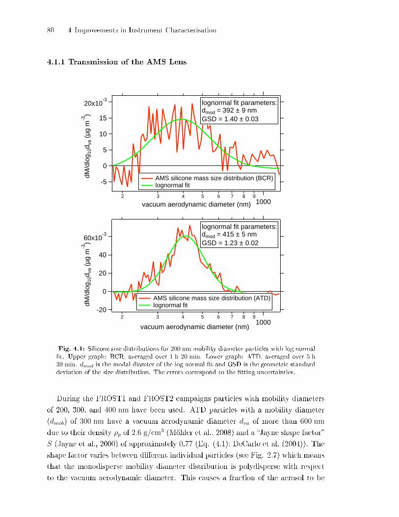
80 4 Improvements in Instrument Characterisation
4.1.1 Transmission of the AMS Lens
60x10-3
40
20
0
-20
dM/d
log 1
0dva
(µg
m-3
)
2 3 4 5 6 7 8 91000
vacuum aerodynamic diameter (nm)
AMS silicone mass size distribution (ATD) lognormal fit
lognormal fit parameters:dmod = 415 ± 5 nmGSD = 1.23 ± 0.02
20x10-3
15
10
5
0
-5
dM/d
log 1
0dva
(µg
m-3
)
2 3 4 5 6 7 8 91000vacuum aerodynamic diameter (nm)
lognormal fit parameters:dmod = 392 ± 9 nmGSD = 1.40 ± 0.03
AMS silicone mass size distribution (BCR) lognormal fit
Fig. 4.1: Silicone size distributions for 200 nm mobility diameter particles with log normal�t. Upper graph: BCR, averaged over 1 h 20 min. Lower graph: ATD, averaged over 5 h39 min. dmod is the modal diamter of the log normal �t and GSD is the geometric standarddeviation of the size distribution. The errors correspond to the �tting uncertainties.
During the FROST1 and FROST2 campaigns particles with mobility diameters
of 200, 300, and 400 nm have been used. ATD particles with a mobility diameter
(dmob) of 300 nm have a vacuum aerodynamic diameter dva of more than 600 nm
due to their density ρp of 2.6 g/cm3 (Möhler et al., 2008) and a �Jayne shape factor�
S (Jayne et al., 2000) of approximately 0.77 (Eq. (4.1); DeCarlo et al. (2004)). The
shape factor varies between di�erent individual particles (see Fig. 2.7) which means
that the monodisperse mobility diameter distribution is polydisperse with respect
to the vacuum aerodynamic diameter. This causes a fraction of the aerosol to be

4.1 Correction Factors 81
1.0
0.8
0.6
0.4
0.2
0.0
a.u.
4 5 6 7 8 91000
2
dva [nm]
transmission ATD 400 nm projected ATD 400 nm corrected ATD 300 nm projected ATD 300 nm corrected
1.0
0.8
0.6
0.4
0.2
0.0
a.u.
4 5 6 7 8 91000
2
dva [nm]
transmission BCR 400 nm projection BCR 400 nm corrected BCR 300 nm projection BCR 300 nm corrected
Fig. 4.2: Transmission correction for BCR and ATD particles. The �gures show theprojected transmission curves as calculated from the �ts in Fig. 4.1 as well as the projectedsize distribution when the transmission of the aerodynamic lens is taken into account.
outside the 100 % transmission range of the AMS inlet. For the 400 nm particles
used during FROST1, this e�ect is even stronger.
dva = Sρp · dmob (4.1)
To get accurate coating thicknesses, this loss factor must be estimated. Due to the
thin coatings of the particles the size distributions measured by the AMS were very
noisy. Furthermore the size calibration above 600 nm has large uncertainties as it is
very �at (see Fig. 2.2). To nevertheless access the size distributions of the 300 and
400 nm particles, some assumptions had to be made: The vacuum aerodynamic mass
size distribution of the ATD was assumed to be lognormally distributed with the
same geometric width independent of the mode diameter (Fig. 4.1). The lognormal
�t to the correctly measured 200 nm particles can be projected to the 300 and
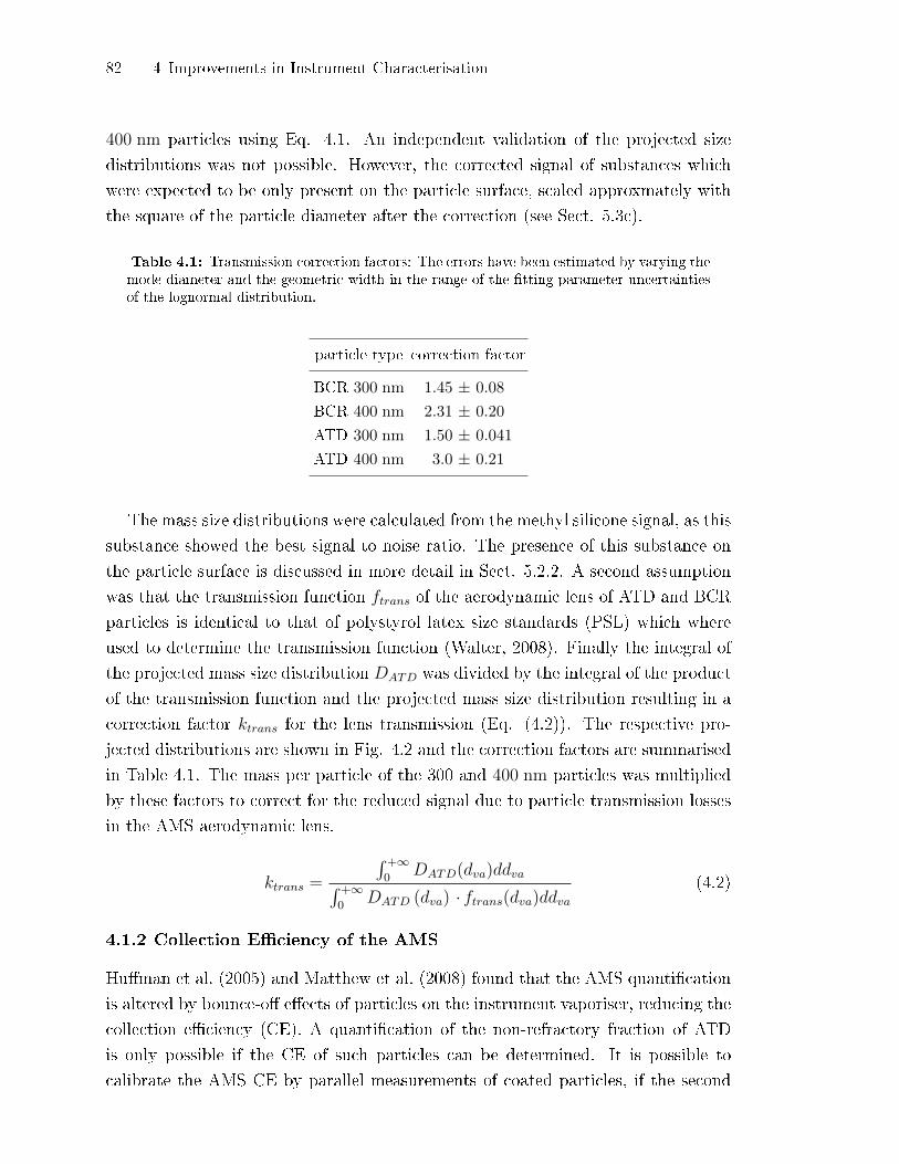
82 4 Improvements in Instrument Characterisation
400 nm particles using Eq. 4.1. An independent validation of the projected size
distributions was not possible. However, the corrected signal of substances which
were expected to be only present on the particle surface, scaled approxmately with
the square of the particle diameter after the correction (see Sect. 5.3c).
Table 4.1: Transmission correction factors: The errors have been estimated by varying themode diameter and the geometric width in the range of the �tting parameter uncertaintiesof the lognormal distribution.
particle type correction factor
BCR 300 nm
BCR 400 nm
ATD 300 nm
ATD 400 nm
1.45 ± 0.08
2.31 ± 0.20
1.50 ± 0.041
3.0 ± 0.21
The mass size distributions were calculated from the methyl silicone signal, as this
substance showed the best signal to noise ratio. The presence of this substance on
the particle surface is discussed in more detail in Sect. 5.2.2. A second assumption
was that the transmission function ftrans of the aerodynamic lens of ATD and BCR
particles is identical to that of polystyrol latex size standards (PSL) which where
used to determine the transmission function (Walter, 2008). Finally the integral of
the projected mass size distribution DATD was divided by the integral of the product
of the transmission function and the projected mass size distribution resulting in a
correction factor ktrans for the lens transmission (Eq. (4.2)). The respective pro-
jected distributions are shown in Fig. 4.2 and the correction factors are summarised
in Table 4.1. The mass per particle of the 300 and 400 nm particles was multiplied
by these factors to correct for the reduced signal due to particle transmission losses
in the AMS aerodynamic lens.
ktrans =
∫ +∞0
DATD(dva)ddva∫ +∞0
DATD (dva) · ftrans(dva)ddva(4.2)
4.1.2 Collection E�ciency of the AMS
Hu�man et al. (2005) and Matthew et al. (2008) found that the AMS quanti�cation
is altered by bounce-o� e�ects of particles on the instrument vaporiser, reducing the
collection e�ciency (CE). A quanti�cation of the non-refractory fraction of ATD
is only possible if the CE of such particles can be determined. It is possible to
calibrate the AMS CE by parallel measurements of coated particles, if the second
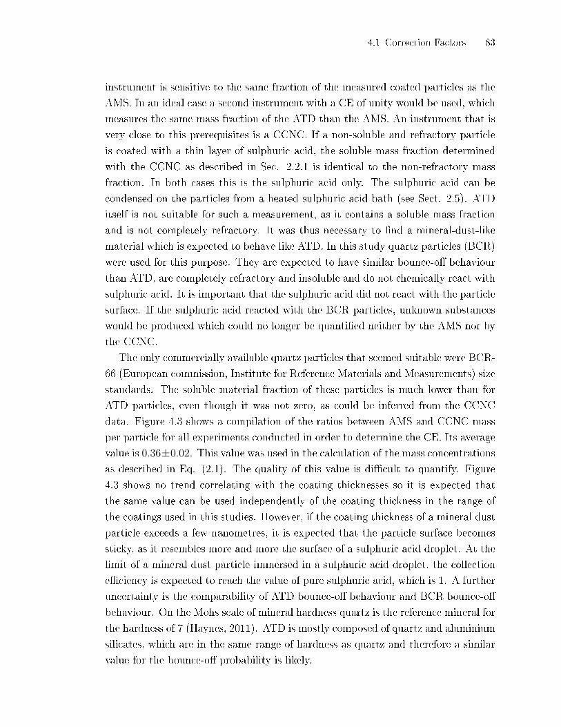
4.1 Correction Factors 83
instrument is sensitive to the same fraction of the measured coated particles as the
AMS. In an ideal case a second instrument with a CE of unity would be used, which
measures the same mass fraction of the ATD than the AMS. An instrument that is
very close to this prerequisites is a CCNC. If a non-soluble and refractory particle
is coated with a thin layer of sulphuric acid, the soluble mass fraction determined
with the CCNC as described in Sec. 2.2.1 is identical to the non-refractory mass
fraction. In both cases this is the sulphuric acid only. The sulphuric acid can be
condensed on the particles from a heated sulphuric acid bath (see Sect. 2.5). ATD
itself is not suitable for such a measurement, as it contains a soluble mass fraction
and is not completely refractory. It was thus necessary to �nd a mineral-dust-like
material which is expected to behave like ATD. In this study quartz particles (BCR)
were used for this purpose. They are expected to have similar bounce-o� behaviour
than ATD, are completely refractory and insoluble and do not chemically react with
sulphuric acid. It is important that the sulphuric acid did not react with the particle
surface. If the sulphuric acid reacted with the BCR particles, unknown substances
would be produced which could no longer be quanti�ed neither by the AMS nor by
the CCNC.
The only commercially available quartz particles that seemed suitable were BCR-
66 (European commission, Institute for Reference Materials and Measurements) size
standards. The soluble material fraction of these particles is much lower than for
ATD particles, even though it was not zero, as could be inferred from the CCNC
data. Figure 4.3 shows a compilation of the ratios between AMS and CCNC mass
per particle for all experiments conducted in order to determine the CE. Its average
value is 0.36±0.02. This value was used in the calculation of the mass concentrationsas described in Eq. (2.1). The quality of this value is di�cult to quantify. Figure
4.3 shows no trend correlating with the coating thicknesses so it is expected that
the same value can be used independently of the coating thickness in the range of
the coatings used in this studies. However, if the coating thickness of a mineral dust
particle exceeds a few nanometres, it is expected that the particle surface becomes
sticky, as it resembles more and more the surface of a sulphuric acid droplet. At the
limit of a mineral dust particle immersed in a sulphuric acid droplet, the collection
e�ciency is expected to reach the value of pure sulphuric acid, which is 1. A further
uncertainty is the comparability of ATD bounce-o� behaviour and BCR bounce-o�
behaviour. On the Mohs scale of mineral hardness quartz is the reference mineral for
the hardness of 7 (Haynes, 2011). ATD is mostly composed of quartz and aluminium
silicates, which are in the same range of hardness as quartz and therefore a similar
value for the bounce-o� probability is likely.

84 4 Improvements in Instrument Characterisation
0.5
0.4
0.3
0.2
0.1
0.0
colle
ctio
n ef
ficie
ncy
200
nm 5
0 °C
200
nm 7
0 °C
300
nm 5
0 °C
300
nm 7
0 °C
300
nm 7
0 °C
WB
300
nm 7
0 °C
TD 2
50°C
300
nm 8
5 °C
300
nm 8
5 °C
300
nm 8
5 °C
TD 1
50°C
300
nm 8
5 °C
TD 1
50°C
300
nm 8
5 °C
TD 2
50 °C
400
nm 5
0 °C
400
nm 7
0 °C
ratio AMS to CCNC mean value (=0.357)
Fig. 4.3: Collection e�ciency (CE) for all experiments using coated BCR particles. Thecategories refer to di�erent experimental conditions. The �rst number is the dmob, the secondthe temperature of the sulphuric acid bath used for the coating. WB indicates humidi�cationof the particles with a water bath and TD indicates the use of a thermodenuder at thetemperature following TD. Every data point was averaged over ∼ 106 particles. The errorbars were calculated from Gaussian error propagation using the standard deviations of themean values for the time series of the mass per particle corresponding to the data pointsand the con�dence intervals of the soluble mass per particle determined with the CCNC.
A collection e�ciency of 0.36 is below the average collection e�ciency of 0.5 which
is commonly used in the AMS community to correct ambient AMS data, when the
exact CE is unknown. However, for pure, dry ammonium sulphate particles, CEs
down to 0.2 have been reported (Matthew et al., 2008). The lowest value for the
CE of a single experiment in this study was not lower than 0.25. Unfortunately no
data for pure ammonium sulphate was collected during the parallel measurements
of the AMS and the CCNC. Therefore it is not possible to check if the CE of 0.2 for
dry ammonium sulphate could be reproduced with the set-up used during FROST.
Together with the measurements to determine the collection e�ciency of the
AMS, some experiments of the FROST1 and the FROST2 campaign were repeated.
The CCNC reproduced the soluble mass per particle for experiments with the same
particle generation settings. However, the AMS did not reproduce the mass load-
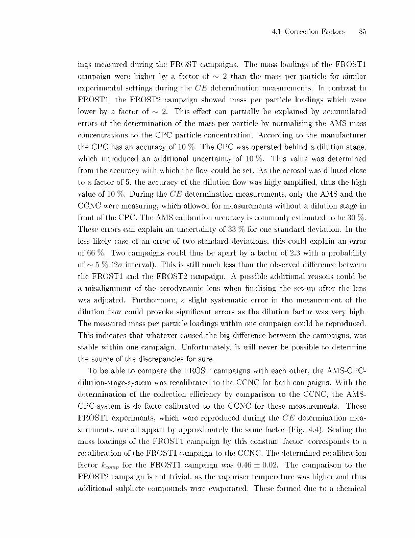
4.1 Correction Factors 85
ings measured during the FROST campaigns. The mass loadings of the FROST1
campaign were higher by a factor of ∼ 2 than the mass per particle for similar
experimental settings during the CE determination measurements. In contrast to
FROST1, the FROST2 campaign showed mass per particle loadings which were
lower by a factor of ∼ 2. This e�ect can partially be explained by accumulated
errors of the determination of the mass per particle by normalising the AMS mass
concentrations to the CPC particle concentration. According to the manufacturer
the CPC has an accuracy of 10 %. The CPC was operated behind a dilution stage,
which introduced an additional uncertainty of 10 %. This value was determined
from the accuracy with which the �ow could be set. As the aerosol was diluted close
to a factor of 5, the accuracy of the dilution �ow was higly ampli�ed, thus the high
value of 10 %. During the CE determination measurements, only the AMS and the
CCNC were measuring, which allowed for measurements without a dilution stage in
front of the CPC. The AMS calibration accuracy is commonly estimated to be 30 %.
These errors can explain an uncertainty of 33 % for one standard deviation. In the
less likely case of an error of two standard deviations, this could explain an error
of 66 %. Two campaigns could thus be apart by a factor of 2.3 with a probability
of ∼ 5 % (2σ interval). This is still much less than the observed di�erence between
the FROST1 and the FROST2 campaign. A possible additional reasons could be
a misalignment of the aerodynamic lens when �nalising the set-up after the lens
was adjusted. Furthermore, a slight systematic error in the measurement of the
dilution �ow could provoke signi�cant errors as the dilution factor was very high.
The measured mass per particle loadings within one campaign could be reproduced.
This indicates that whatever caused the big di�erence between the campaigns, was
stable within one campaign. Unfortunately, it will never be possible to determine
the source of the discrepancies for sure.
To be able to compare the FROST campaigns with each other, the AMS-CPC-
dilution-stage-system was recalibrated to the CCNC for both campaigns. With the
determination of the collection e�ciency by comparison to the CCNC, the AMS-
CPC-system is de facto calibrated to the CCNC for these measurements. Those
FROST1 experiments, which were reproduced during the CE determination mea-
surements, are all appart by approximately the same factor (Fig. 4.4). Scaling the
mass loadings of the FROST1 campaign by this constant factor, corresponds to a
recalibration of the FROST1 campaign to the CCNC. The determined recalibration
factor kcomp for the FROST1 campaign was 0.46 ± 0.02. The comparison to the
FROST2 campaign is not trivial, as the vaporiser temperature was higher and thus
additional sulphate compounds were evaporated. These formed due to a chemical

86 4 Improvements in Instrument Characterisation
1000
800
600
400
200
0
FR
OS
T /g
/par
ticle
x10
-18
4003002001000reference /g/particle x10
-18
Least orthogonal distance fitslope = 2.18 ± 0.08
Resulting correction factor: 0.46 ± 0.02
Fig. 4.4: Comparison of the results of the measurements pepeated during the CE deter-mination measurements to the FROST1 campaign.
reaction of the sulphuric acid with the ATD surface (Sect. 5.2.4) and cannot be eas-
ily seperated from the sulphuric acid in the mass spectrum. However, for a coating
temperature of 85 ◦C the coating is thick enough for most of the sulphuric acid to
remain on the particle surface without chemical reaction and thus this experiment
can be used for comparison. This yielded a correction factor of 2.2 ± 0.3 for the
FROST2 campaign.
The CE determined in this section is only useful in connection with the factors
kcomp. Thus it is not clear, how accurate the value of the CE is. It is important
to notice that only one correction factor was applied per campaign. It is thus
still possible to compare the CCNC measurements to the AMS measurements as the
determined quantities were not forced to be equal by the recalibration. Furthermore,
the factors applied are real calibration factors with the attempt to yield correct
values of the mass per particle determined with the AMS. They are not simple
scaling factors (�fudge factors�) to force the results of the FROST1 and the FROST2
campaign to agree.
4.1.3 AMS Relative Ionisation E�ciency
Some measurements of pure ammonium sulphate and ammonium nitrate were per-
formed. They revealed that the stoichiometric ratios between ammonium and sul-
phate and nitrate respectively are not reproduced correctly by the AMS when using
values from literature for the relative ionisation e�ciencies of sulphate and ammo-
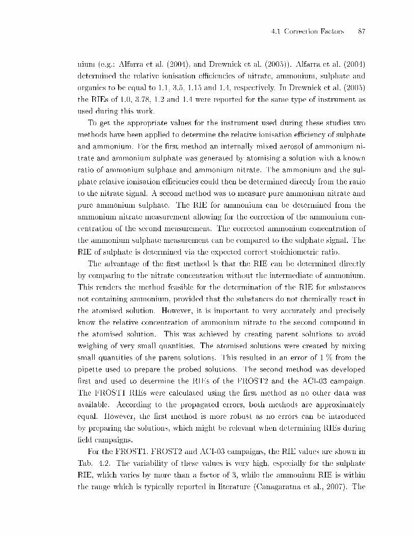
4.1 Correction Factors 87
nium (e.g.: Alfarra et al. (2004), and Drewnick et al. (2005)). Alfarra et al. (2004)
determined the relative ionisation e�ciencies of nitrate, ammonium, sulphate and
organics to be equal to 1.1, 3.5, 1.15 and 1.4, respectively. In Drewnick et al. (2005)
the RIEs of 1.0, 3.78, 1.2 and 1.4 were reported for the same type of instrument as
used during this work.
To get the appropriate values for the instrument used during these studies two
methods have been applied to determine the relative ionisation e�ciency of sulphate
and ammonium. For the �rst method an internally mixed aerosol of ammonium ni-
trate and ammonium sulphate was generated by atomising a solution with a known
ratio of ammonium sulphate and ammonium nitrate. The ammonium and the sul-
phate relative ionisation e�ciencies could then be determined directly from the ratio
to the nitrate signal. A second method was to measure pure ammonium nitrate and
pure ammonium sulphate. The RIE for ammonium can be determined from the
ammonium nitrate measurement allowing for the correction of the ammonium con-
centration of the second measurement. The corrected ammonium concentration of
the ammonium sulphate measurement can be compared to the sulphate signal. The
RIE of sulphate is determined via the expected correct stoichiometric ratio.
The advantage of the �rst method is that the RIE can be determined directly
by comparing to the nitrate concentration without the intermediate of ammonium.
This renders the method feasible for the determination of the RIE for substances
not containing ammonium, provided that the substances do not chemically react in
the atomised solution. However, it is important to very accurately and precisely
know the relative concentration of ammonium nitrate to the second compound in
the atomised solution. This was achieved by creating parent solutions to avoid
weighing of very small quantities. The atomised solutions were created by mixing
small quantities of the parent solutions. This resulted in an error of 1 % from the
pipette used to prepare the probed solutions. The second method was developed
�rst and used to determine the RIEs of the FROST2 and the ACI-03 campaign.
The FROST1 RIEs were calculated using the �rst method as no other data was
available. According to the propagated errors, both methods are approximately
equal. However, the �rst method is more robust as no errors can be introduced
by preparing the solutions, which might be relevant when determining RIEs during
�eld campaigns.
For the FROST1, FROST2 and ACI-03 campaigns, the RIE values are shown in
Tab. 4.2. The variability of these values is very high, especially for the sulphate
RIE, which varies by more than a factor of 3, while the ammonium RIE is within
the range which is typically reported in literature (Canagaratna et al., 2007). The
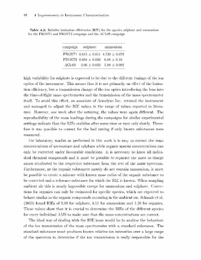
88 4 Improvements in Instrument Characterisation
Table 4.2: Relative ionisation e�ciencies (RIE) for the species sulphate and ammoniumfor the FROST1 and FROST2 campaign and the ACI-03 campaign
campaign sulphate ammonium
FROST1
FROST2
ACI-03
0.615 ± 0.011
0.694 ± 0.026
2.06 ± 0.032
4.739 ± 0.079
6.08 ± 0.16
5.88 ± 0.092
high variability for sulphate is expected to be due to the di�erent tunings of the ion
optics of the instrument. This means that it is not primarily an e�ect of the ionisa-
tion e�ciency, but a transmission change of the ion optics introducing the ions into
the time-of-�ight mass spectrometer and the transmission of the mass spectrometer
itself. To avoid this e�ect, an associate of Aerodyne Inc. retuned the instrument
and managed to adjust the RIE values in the range of values reported in litera-
ture. However, one week after the retuning, the values were again di�erent. The
reproducibility of the mass loadings during the campaigns for similar experimental
settings indicate that the RIEs stabilise after some time or vary only slowly. There-
fore it was possible to correct for the bad tuning if only known substances were
measured.
For laboratory studies as performed in this work it is easy to correct the mass
concentrations of ammonium and sulphate while organic species concentrations can
only be corrected under favourable conditions. It is necessary to know all indivi-
dual chemical compounds and it must be possible to separate the mass to charge
ratios attributed to the respective substance from the rest of the mass spectrum.
Furthermore, as the organic substances mostly do not contain ammonium, it must
be possible to create a mixture with known mass ratios of the organic substance to
be corrected and a reference substance for which the RIE is known. When sampling
ambient air this is nearly impossible except for ammonium and sulphate. Correc-
tions for organics can only be estimated for speci�c species, which are expected to
behave similar as the organic compounds occurring in the ambient air. Schmale et al.
(2010) found RIEs of 0.98 for sulphate, 3.11 for ammonium and 1.76 for organics.
These values show that it is crucial to determine the RIEs of the di�erent species
for every individual AMS to make sure that the mass concentrations are correct.
The ideal way of dealing with the RIE issue would be to analyse the behaviour
of the ion transmission of the mass spectrometer with a standard substance. The
standard substance must produces known relative ion intensities over a large range
of the spectrum to determine if the ion transmission is really responsible for the
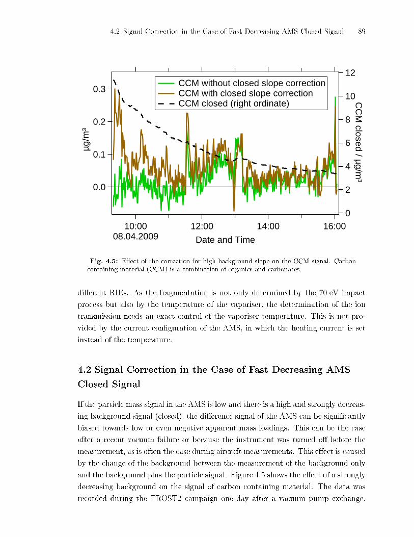
4.2 Signal Correction in the Case of Fast Decreasing AMS Closed Signal 89
0.3
0.2
0.1
0.0
µg/m
³
10:0008.04.2009
12:00 14:00 16:00
Date and Time
12
10
8
6
4
2
0
CC
M closed / µg/m
³
CCM without closed slope correction CCM with closed slope correction CCM closed (right ordinate)
Fig. 4.5: E�ect of the correction for high background slope on the CCM signal. Carboncontaining material (CCM) is a combination of organics and carbonates.
di�erent RIEs. As the fragmentation is not only determined by the 70 eV impact
process but also by the temperature of the vaporiser, the determination of the ion
transmission needs an exact control of the vaporiser temperature. This is not pro-
vided by the current con�guration of the AMS, in which the heating current is set
instead of the temperature.
4.2 Signal Correction in the Case of Fast Decreasing AMS
Closed Signal
If the particle mass signal in the AMS is low and there is a high and strongly decreas-
ing background signal (closed), the di�erence signal of the AMS can be signi�cantly
biased towards low or even negative apparent mass loadings. This can be the case
after a recent vacuum failure or because the instrument was turned o� before the
measurement, as is often the case during aircraft measurements. This e�ect is caused
by the change of the background between the measurement of the background only
and the background plus the particle signal. Figure 4.5 shows the e�ect of a strongly
decreasing background on the signal of carbon containing material. The data was
recorded during the FROST2 campaign one day after a vacuum pump exchange.

90 4 Improvements in Instrument Characterisation
Both campaigns CE = 0.36
FROST1 Recalibration
to CCNC factor:
kcomp = 0.46
FROST2 Recalibration
to CCNC factor:
kcomp = 2.2
200 nm ktrans = 1
300 nm ktrans = 1.5
400 nm ktrans = 3
300 nm ktrans = 1.5
Sulphate RIE = 0.615
Ammonium RIE = 4.74
Sulphate RIE = 0.694
Ammonium RIE = 6.08
AMS lens transmission
Relative Ionisation Efficiency
Calibration factor to CCNC
Collection Efficiency
Fig. 4.6: Summary of the correction factors which need to be applied to the di�erent AMSmass loadings to get correct quantitative results.
The black dashed line shows the background signal, which changes between two
runs (1 run = 60 s) in the order of magnitude of the real signal. Because of the high
change in the background, the real signal is underestimated as shown in the green
curve. To correct for this e�ect, the closed signal was smoothed and the background
change between two consecutive sample runs was calculated. As the instrument
is switching several times between open and closed during one recording run, the
change has to be scaled down to half of one closed-open period before subtraction.
For example, if during one recording run three open closed periods are performed,
the amount added to the di�erence signal is equal to 1/6 of the background change
between two runs. A drawback of the method is a strong increase of the noise. This
technique was applied to those signals which were recorded shortly after a vacuum
failure. As shown in Fig. 4.5 the �rst three hours of this data set are clearly a�ected
by this high background: The uncorrected signal is partly below zero. After about
�ve hours, the instrumental background had markedly decreased, and the di�erence
between the uncorrected and the corrected signal became negligible.
4.3 Summary of the Correction Factors 91
4.3 Summary of the Correction Factors
The correction factors determined in this chapter are summarised in Fig.4.6. To
get an accurate determination of the mass per particle for sulphate and ammo-
nium, all the factors shown in Fig. 4.6 must be applied. The collection e�ciency
for BCR-particles, which is expected to be the same as for ATD, is equal for both
FROST campaigns. The recalibration factor to achieve comparability between the
measurement campaigns (kcomp) di�ers for both FROST campaigns. The AMS lens
transmission correction factors (ktrans) are applied to the 300 and 400 nm particle
mass loadings. The exact RIE could only be determined for sulphate and ammo-
nium. The correction factors were applied to all measurements of these species.
For di�erent species, like organics, the RIE could not be determined and therefore
the default values of the fragmentation table were used. It is thus likely that the
mass per particle for these substances is not quantitatively correct. However, the
conclusions drawn in this thesis do not need a quanti�cation of organics.
For the campaign ACI-03, only the RIEs were determined. The CE and the lens
transmission could not be calculated. No recalibration to a CCNC was performed. In
Chapt. 6 the attempts to correct the data from the ACI-03 campaign are discussed.

5
Laboratory Studies on the Ice Nucleation E�ciency
of ATD
The main goal of this work was to determine the e�ect of thin coatings on the IN
and CCN behaviour of mineral dust particles. During the FROST1 and FROST2
campaigns in Leipzig, ATD was coated with sulphuric acid and optionally humidi�ed
and/or heated to determine the e�ect of these treatments on the IN- and CCN-
e�ciency of mineral dust particles. In the following it is shown that coating particles
with sulphuric acid not only covers the particle surface, but also leads to reactions
with the particle surface which irreversibly reduces the IN ability of ATD. The
results presented in this chapter have been published in Reitz et al. (2011).
5.1 Experimental Set-up
Figure 5.1 shows the experimental set-up of the FROST campaigns. The left side
shows the particle generation section and the right side shows the aerosol charac-
terisation section. The ATD particles are suspended in a �uidized bed generator
(TSI 3400A, TSI Inc., St. Paul, Minnesota, USA) which is immediately followed
by a multi stage impactor. The impactor removes the large particle fraction of the
dispersed aerosol in order to reduce the multiply charged particle fraction when
selecting the diameter of the particles with a di�erential mobility analyser (DMA)
at the end of the generation set-up. Mobility diameters of 200 nm, 300 nm, and
400 nm were selected. The 50 % cut-o� of the impactor is set to 560 nm aerody-
namic diameter when 200 nm or 300 nm mobility diameter particles were selected
and to 1 µm when the 400 nm mobility diameter particles were selected. Table 5.1
shows the mobility diameter dmob, the volume equivalent diameter dve and the aero-
dynamic diameter da of ATD for singly and doubly charged particles for the three
diameters used in this study. For dmob = 300 nm the doubly charged particles were
e�ciently suppressed as their aerodynamic size is clearly higher than 560 nm. The
size fraction that results in singly charged particles could pass the impactor stages
without being reduced. When using particles of 200 nm and 400 nm it is expected

94 5 Laboratory Studies on the Ice Nucleation E�ciency of ATD
Fluidized bed generator with
impactor
Sulphuric acid bath
Water bath
Dryer
Thermodenuder
DMA
AMS
CPC
CCNC
IN-counter
Additional instrumentation
Possible NH3 addition LACIS
Fig. 5.1: Experimental set-up of the FROST campaigns. The sections between the �uidizedbed generator and the DMA can be bypassed.
that some doubly charged particles passed the DMA. Because of this technical rea-
son, the 300 nm mobility diameter particles were studied most extensively and were
the only particle size used during FROST2.
Doubly charged particles would have an increased diameter and thus also provide
more surface than singly charged particles of the same mobility diameter. The
increased diameter would cause the particles to be transmitted less e�ciently by the
aerodynamic lens of the AMS. Furtehrmore the increased surface would likely cause
multiply chared particles to carry more coating material. The CPC however would
count the doubly charged particles correctly independent of their size. Whether
multiply charged particles cause a bias to higher or lower values depends on the
ratio of the additional surface material carried by these particles and the loss due to
non-optimal transmission into the AMS. For 200 nm mobility diameter, the doubly
charged particles have a size of 323 nm and thus a transmission loss of slightly more
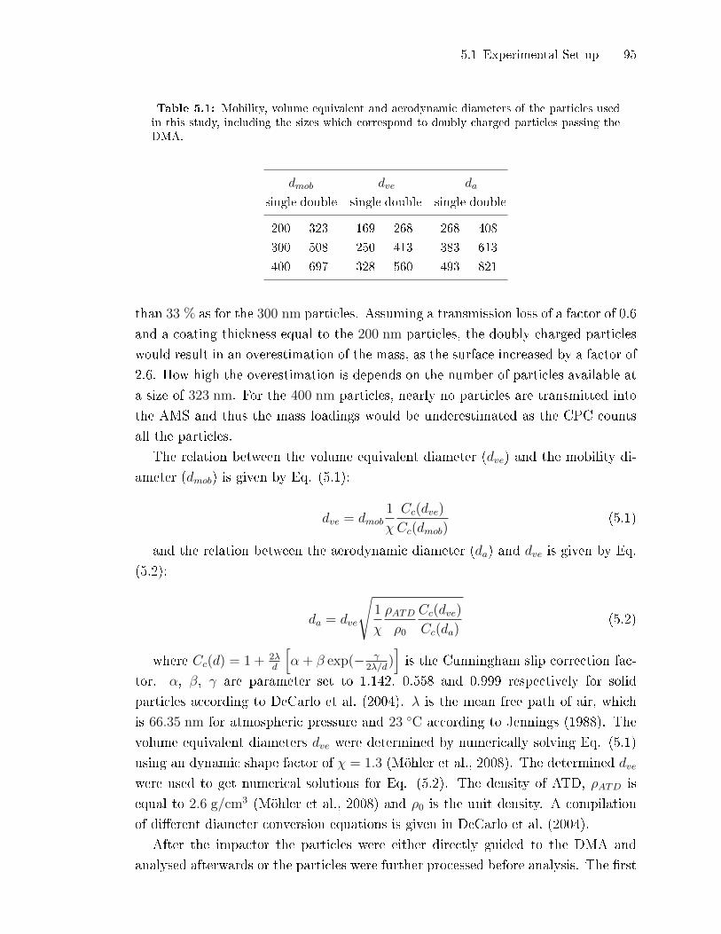
5.1 Experimental Set-up 95
Table 5.1: Mobility, volume equivalent and aerodynamic diameters of the particles usedin this study, including the sizes which correspond to doubly charged particles passing theDMA.
dmob dve da
single double single double single double
200 323 169 268 268 408
300 508 250 413 383 613
400 697 328 560 493 821
than 33 % as for the 300 nm particles. Assuming a transmission loss of a factor of 0.6
and a coating thickness equal to the 200 nm particles, the doubly charged particles
would result in an overestimation of the mass, as the surface increased by a factor of
2.6. How high the overestimation is depends on the number of particles available at
a size of 323 nm. For the 400 nm particles, nearly no particles are transmitted into
the AMS and thus the mass loadings would be underestimated as the CPC counts
all the particles.
The relation between the volume equivalent diameter (dve) and the mobility di-
ameter (dmob) is given by Eq. (5.1):
dve = dmob1
χ
Cc(dve)
Cc(dmob)(5.1)
and the relation between the aerodynamic diameter (da) and dve is given by Eq.
(5.2):
da = dve
√1
χ
ρATDρ0
Cc(dve)
Cc(da)(5.2)
where Cc(d) = 1 + 2λd
[α + β exp(− γ
2λ/d)]is the Cunningham slip correction fac-
tor. α, β, γ are parameter set to 1.142, 0.558 and 0.999 respectively for solid
particles according to DeCarlo et al. (2004). λ is the mean free path of air, which
is 66.35 nm for atmospheric pressure and 23 ◦C according to Jennings (1988). The
volume equivalent diameters dve were determined by numerically solving Eq. (5.1)
using an dynamic shape factor of χ = 1.3 (Möhler et al., 2008). The determined dve
were used to get numerical solutions for Eq. (5.2). The density of ATD, ρATD is
equal to 2.6 g/cm3 (Möhler et al., 2008) and ρ0 is the unit density. A compilation
of di�erent diameter conversion equations is given in DeCarlo et al. (2004).
After the impactor the particles were either directly guided to the DMA and
analysed afterwards or the particles were further processed before analysis. The �rst
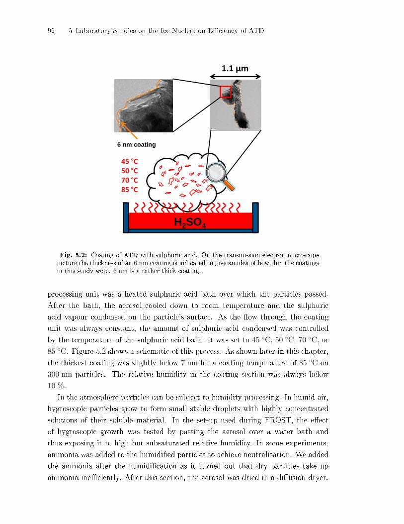
96 5 Laboratory Studies on the Ice Nucleation E�ciency of ATD
H2SO4
6 nm coating
45 °C 50 °C 70 °C 85 °C
1.1 µm
Fig. 5.2: Coating of ATD with sulphuric acid. On the transmission electron microscopepicture the thickness of an 6 nm coating is indicated to give an idea of how thin the coatingsin this study were. 6 nm is a rather thick coating.
processing unit was a heated sulphuric acid bath over which the particles passed.
After the bath, the aerosol cooled down to room temperature and the sulphuric
acid vapour condensed on the particle's surface. As the �ow through the coating
unit was always constant, the amount of sulphuric acid condensed was controlled
by the temperature of the sulphuric acid bath. It was set to 45 ◦C, 50 ◦C, 70 ◦C, or
85 ◦C. Figure 5.2 shows a schematic of this process. As shown later in this chapter,
the thickest coating was slightly below 7 nm for a coating temperature of 85 ◦C on
300 nm particles. The relative humidity in the coating section was always below
10 %.
In the atmosphere particles can be subject to humidity processing. In humid air,
hygroscopic particles grow to form small stable droplets with highly concentrated
solutions of their soluble material. In the set-up used during FROST, the e�ect
of hygroscopic growth was tested by passing the aerosol over a water bath and
thus exposing it to high but subsaturated relative humidity. In some experiments,
ammonia was added to the humidi�ed particles to achieve neutralisation. We added
the ammonia after the humidi�cation as it turned out that dry particles take up
ammonia ine�ciently. After this section, the aerosol was dried in a di�usion dryer.
5.2 Results and Discussion 97
The last processing step was a thermodenuder in order to remove the semi-volatile
fraction of the aerosol. It was typically set to 250 ◦C but in some experiments also
45 ◦C and 70 ◦C were used. It turned out that in addition to removing the semi-
volatile fraction of the particles, the thermodenuder provoked a heat treatment of
the particles. This heat treatment accelerated the reactions taking place on the
particles' surface.
After the particles were prepared, they were analysed by a CCNC, an IN counter,
LACIS and the AMS. A CPC was operated parallel to the AMS and the AMS mass
concentrations were normalised to the particle number concentrations. This was
possible as the aerosol was monodisperse and therefore it was expected that all
particles have approximately the same surface for the sulphuric acid to condense on.
More details on the instruments are provided in Sect. 2.
5.2 Results and Discussion
5.2.1 Uncoated Dust Particles
In a �rst analysis the AMS mass spectra of pure ATD recorded at 600 ◦C and
820 ◦C AMS vaporiser temperature were analysed to obtain information on the non-
refractory fraction of the ATD. Afterwards the e�ect of coating the particles with
sulphuric acid is shown. The unit mass resolution spectra shown in Fig. 5.3a to Fig.
5.3c are not corrected for any e�ects like collection e�ciency or inlet transmission.
Furthermore, the relative ionisation e�ciencies were not applied in these �gures. The
peak heights shown are thus in nitrate equivalent mass, meaning that they show the
concentration the species would have if they had the same ionisation e�ciency as
the nitrate ions the instrument was calibrated to. However, for the quanti�cation
of the coating mass per particle, all correction and conversion factors have to be
applied. The calculation of the unit mass resolution spectra is described in Sect.
2.1.5.
Figure 5.3a shows the AMS mass spectrum of uncoated ATD measured with an
AMS vaporiser temperature of 600 ◦C. Except for the grey peaks, which correspond
to air compounds, no mass to charge ratios show a high signal. As expected, the
core material of the ATD, which has, according to the manufacturer, an evaporation
temperature of 1615± 75 ◦C, cannot be detected. The only peaks which are clearly
above the surrounding noise are at mass to charge ratios of 55, 56 and 57, which cor-
respond to typical organic fragments, and at 73 and 147, which can be attributed to
methyl silicone. The standard species �organics�, labelled as �Org� in the AMS user
community, was renamed to �carbon containing material� (CCM), as it also covers

98 5 Laboratory Studies on the Ice Nucleation E�ciency of ATD
10-6
10-5
10-4
10-3
10-2
10-1
100
101
102
mas
s co
ncen
trat
ion
/ µg/
m³
14012010080604020m/z
Air Water Nitrate Sulphate CCM Ammonium Chloride Other
55 56 57
73 (silicone)
147 (silicone)
Fig. 5.3a: Average AMS mass spectrum for unprocessed ATD during the FROST1 cam-paign. Notable are the peaks at m/z 73 and 147 that can be attributed to methyl siliconecontaminant.
silicone and carbonates, as shown in the following. The source of the silicone could
not be clari�ed completely. The �rst possible source that was checked was whether
conductive black silicone tubing was used. Timko et al. (2009),Yu et al. (2009), and
Schneider et al. (2006) reported this type of tubing to cause these contaminations.
However, it turned out that only one very short (≈ 30 cm) connection was made out
of silicone. The rest of the set-up only contained stainless steel tubings. Removing
this short silicone connection did not reduce the silicone signal. The impactor stages
after the suspension of the ATD were covered with silicone grease, but removing the
impactor in addition to the silicone tubing did also not remove the silicone signal
from the ATD. As a �nal test, the ATD was directly sampled from a stainless steel
bottle which was �lled with compressed air. The ATD was introduced into the bot-
tle and the bottle was shaken to mechanically resuspend the particles. Even in this
experiment the silicone signal was detected. It can therefore be concluded that the
silicone was introduced by the compressed air, which might have used silicone grease
in the pumps or it was already present on the ATD after the manufacturing process.
For the subsequent analysis it was treated as a known contaminant.
In Fig. 5.3b, the AMS mass spectrum of pure ATD evaporated at 820 ◦C is
presented. The organic peaks at m/z 55, 56, and 57 are lower, probably due to
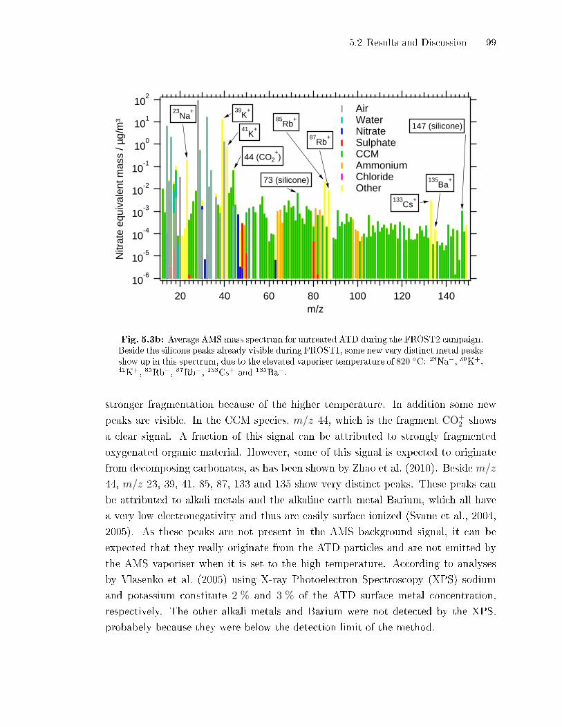
5.2 Results and Discussion 99
10-6
10-5
10-4
10-3
10-2
10-1
100
101
102
Nitr
ate
equi
vale
nt m
ass
/ µg/
m³
14012010080604020m/z
Air Water Nitrate Sulphate CCM Ammonium Chloride Other
23Na
+
44 (CO2+)
39K
+
41K
+
73 (silicone)
85Rb
+
87Rb
+
133Cs
+
135Ba
+
147 (silicone)
Fig. 5.3b: Average AMS mass spectrum for untreated ATD during the FROST2 campaign.Beside the silicone peaks already visible during FROST1, some new very distinct metal peaksshow up in this spectrum, due to the elevated vaporiser temperature of 820 ◦C: 23Na+, 39K+,41K+, 85Rb+, 87Rb+, 133Cs+ and 135Ba+.
stronger fragmentation because of the higher temperature. In addition some new
peaks are visible. In the CCM species, m/z 44, which is the fragment CO+2 shows
a clear signal. A fraction of this signal can be attributed to strongly fragmented
oxygenated organic material. However, some of this signal is expected to originate
from decomposing carbonates, as has been shown by Zhao et al. (2010). Beside m/z
44, m/z 23, 39, 41, 85, 87, 133 and 135 show very distinct peaks. These peaks can
be attributed to alkali metals and the alkaline earth metal Barium, which all have
a very low electronegativity and thus are easily surface ionized (Svane et al., 2004,
2005). As these peaks are not present in the AMS background signal, it can be
expected that they really originate from the ATD particles and are not emitted by
the AMS vaporiser when it is set to the high temperature. According to analyses
by Vlasenko et al. (2005) using X-ray Photoelectron Spectroscopy (XPS) sodium
and potassium constitute 2 % and 3 % of the ATD surface metal concentration,
respectively. The other alkali metals and Barium were not detected by the XPS,
probabely because they were below the detection limit of the method.
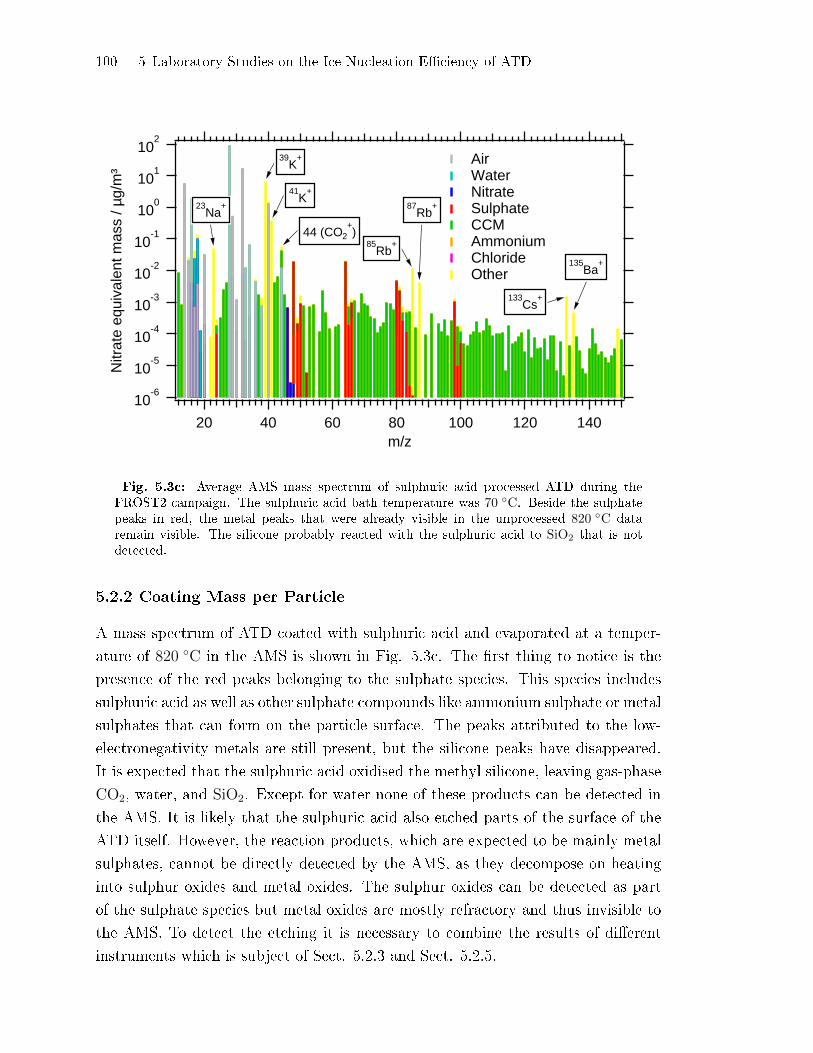
100 5 Laboratory Studies on the Ice Nucleation E�ciency of ATD
10-6
10-5
10-4
10-3
10-2
10-1
100
101
102
Nitr
ate
equi
vale
nt m
ass
/ µg/
m³
14012010080604020m/z
Air Water Nitrate Sulphate CCM Ammonium Chloride Other
23Na
+
39K
+
41K
+
44 (CO2+)
85Rb
+
87Rb
+
133Cs
+
135Ba
+
Fig. 5.3c: Average AMS mass spectrum of sulphuric acid processed ATD during theFROST2 campaign. The sulphuric acid bath temperature was 70 ◦C. Beside the sulphatepeaks in red, the metal peaks that were already visible in the unprocessed 820 ◦C dataremain visible. The silicone probably reacted with the sulphuric acid to SiO2 that is notdetected.
5.2.2 Coating Mass per Particle
A mass spectrum of ATD coated with sulphuric acid and evaporated at a temper-
ature of 820 ◦C in the AMS is shown in Fig. 5.3c. The �rst thing to notice is the
presence of the red peaks belonging to the sulphate species. This species includes
sulphuric acid as well as other sulphate compounds like ammonium sulphate or metal
sulphates that can form on the particle surface. The peaks attributed to the low-
electronegativity metals are still present, but the silicone peaks have disappeared.
It is expected that the sulphuric acid oxidised the methyl silicone, leaving gas-phase
CO2, water, and SiO2. Except for water none of these products can be detected in
the AMS. It is likely that the sulphuric acid also etched parts of the surface of the
ATD itself. However, the reaction products, which are expected to be mainly metal
sulphates, cannot be directly detected by the AMS, as they decompose on heating
into sulphur oxides and metal oxides. The sulphur oxides can be detected as part
of the sulphate species but metal oxides are mostly refractory and thus invisible to
the AMS. To detect the etching it is necessary to combine the results of di�erent
instruments which is subject of Sect. 5.2.3 and Sect. 5.2.5.
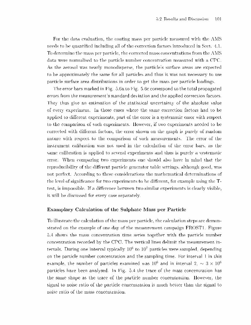
5.2 Results and Discussion 101
For the data evaluation, the coating mass per particle measured with the AMS
needs to be quanti�ed including all of the correction factors introduced in Sect. 4.1.
To determine the mass per particle, the corrected mass concentrations from the AMS
data were normalised to the particle number concentration measured with a CPC.
As the aerosol was nearly monodisperse, the particle's surface areas are expected
to be approximately the same for all particles and thus it was not necessary to use
particle surface area distributions in order to get the mass per particle loadings.
The error bars marked in Fig. 5.6a to Fig. 5.6c correspond to the total propagated
errors from the measurement's standard deviation and the applied correction factors.
They thus give an estimation of the statistical uncertainty of the absolute value
of every experiment. In those cases where the same correction factors had to be
applied to di�erent experiments, part of the error is a systematic error with respect
to the comparison of such experiments. However, if two experiments needed to be
corrected with di�erent factors, the error shown on the graph is purely of random
nature with respect to the comparison of such measurements. The error of the
instrument calibration was not used in the calculation of the error bars, as the
same calibration is applied to several experiments and thus is purely a systematic
error. When comparing two experiments one should also have in mind that the
reproducibility of the di�erent particle generator table settings, although good, was
not perfect. According to these considerations the mathematical determinations of
the level of signi�cance for two experiments to be di�erent, for example using the T-
test, is impossible. If a di�erence between two similar experiments is clearly visible,
it will be discussed for every case separately.
Examplary Calculation of the Sulphate Mass per Particle
To illustrate the calculation of the mass per particle, the calculation steps are demon-
strated on the example of one day of the measurement campaign FROST1. Figure
5.4 shows the mass concentration time series together with the particle number
concentration recorded by the CPC. The vertical lines delimit the measurement in-
tervals. During one interval typically 106 to 107 particles were sampled, depending
on the particle number concentration and the sampling time. For interval 1 in this
example, the number of particles examined was 106 and in interval 2, ∼ 3 × 10⁶
particles have been analysed. In Fig. 5.4 the trace of the mass concentration has
the same shape as the trace of the particle number concentration. However, the
signal to noise ratio of the particle concentration is much better than the signal to
noise ratio of the mass concentration.
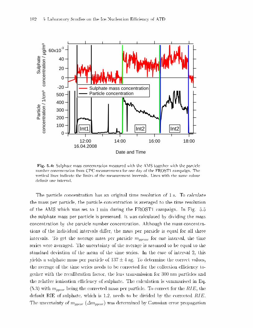
102 5 Laboratory Studies on the Ice Nucleation E�ciency of ATD
60x10-3
40
20
0
-20
Sul
phat
eco
ncen
trat
ion
/ µg/
m³
12:0016.04.2008
14:00 16:00 18:00
Date and Time
500
400
300
200
100
0
Par
ticle
conc
entr
atio
n / 1
/cm
³1.0
0.8
0.6
0.4
0.2
Sulphate mass concentration Particle concentration
Int1 Int2 Int2
Fig. 5.4: Sulphate mass concentration measured with the AMS together with the particlenumber concentration from CPC measurements for one day of the FROST1 campaign. Thevertical lines indicate the limits of the measurement intervals. Lines with the same colourdelimit one interval.
The particle concentration has an original time resolution of 1 s. To calculate
the mass per particle, the particle concentration is averaged to the time resolution
of the AMS which was set to 1 min during the FROST1 campaign. In Fig. 5.5
the sulphate mass per particle is presented. It was calculated by dividing the mass
concentration by the particle number concentration. Although the mass concentra-
tions of the individual intervals di�er, the mass per particle is equal for all three
intervals. To get the average mass per particle mppraw for one interval, the time
series were averaged. The uncertainty of the average is assumed to be equal to the
standard deviation of the mean of the time series. In the case of interval 2, this
yields a sulphate mass per particle of 137± 4 ag. To determine the correct values,
the average of the time series needs to be corrected for the collection e�ciency to-
gether with the recalibration factor, the lens transmission for 300 nm particles and
the relative ionisation e�ciency of sulphate. The calculation is summarised in Eq.
(5.3) with mppcor being the corrected mass per particle. To correct for the RIE, the
default RIE of sulphate, which is 1.2, needs to be divided by the corrected RIE.
The uncertainty of mppcor (∆mppcor) was determined by Gaussian error propagation
5.2 Results and Discussion 103
400
300
200
100
0
-100
Sul
phat
e ag
/par
ticle
12:0016.04.2008
14:00 16:00 18:00
Date and Time
Sulphate per particle
Int1
Exp2
Int2 Int3
Fig. 5.5: Sulphate mass per particle concentration for the same day as shown in Fig. 5.4.The mass per particle was calculated by normalising the mass concentrations measured withthe AMS to the particle number concentrations from CPC measurements. The vertical linesindicate the limits of the measurement intervals. Lines with the same colour delimit oneinterval.
using Eq. (5.6). The resulting mppcor is 516± 42 ag. To get the values for a certain
set of experimental conditions, in this case the intervals Int1 to Int3, the weighted
average of the individual intervals was calculated. The corresponding value is shown
in Fig. 5.6a as experiment 11.
mppcor = CE−1 · kcomp · ktrans ·RIE (default)
RIE·mppraw (5.3)
= 0.36−1 · 0.46 · 1.5 · 1.2
0.615· 137 ag (5.4)
= 516 ag (5.5)
∆mppcor = mppcor ·
√(∆CE
CE
)2
+
(∆kcompkcomp
)2
+
(∆ktransktrans
)2
+
(∆RIE
RIE
)2
(5.6)
= 516 ag ·
√(0.02
0.36
)2
+
(0.02
0.46
)2
+
(0.041
1.5
)2
+
(0.011
0.615
)2
+
(4
137
)2
(5.7)
= 42 ag (5.8)
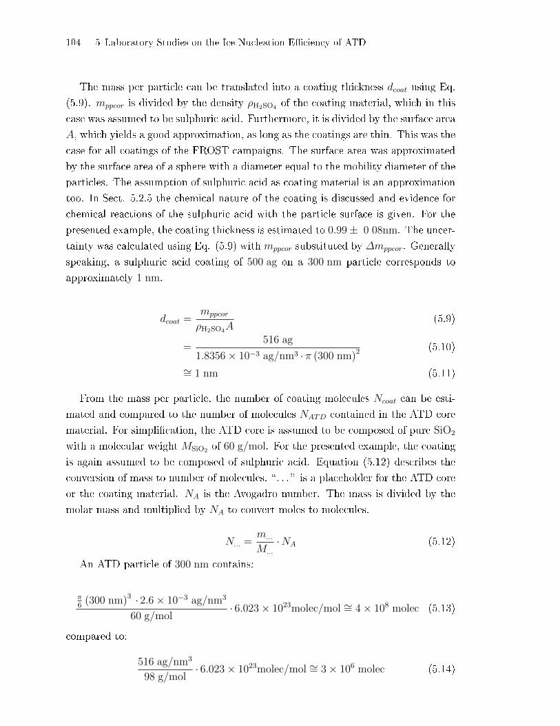
104 5 Laboratory Studies on the Ice Nucleation E�ciency of ATD
The mass per particle can be translated into a coating thickness dcoat using Eq.
(5.9). mppcor is divided by the density ρH2SO4 of the coating material, which in this
case was assumed to be sulphuric acid. Furthermore, it is divided by the surface area
A, which yields a good approximation, as long as the coatings are thin. This was the
case for all coatings of the FROST campaigns. The surface area was approximated
by the surface area of a sphere with a diameter equal to the mobility diameter of the
particles. The assumption of sulphuric acid as coating material is an approximation
too. In Sect. 5.2.5 the chemical nature of the coating is discussed and evidence for
chemical reactions of the sulphuric acid with the particle surface is given. For the
presented example, the coating thickness is estimated to 0.99± 0 08nm. The uncer-
tainty was calculated using Eq. (5.9) with mppcor substituted by ∆mppcor. Generally
speaking, a sulphuric acid coating of 500 ag on a 300 nm particle corresponds to
approximately 1 nm.
dcoat =mppcor
ρH2SO4A(5.9)
=516 ag
1.8356× 10⁻³ ag/nm3 ·π (300 nm)2(5.10)
∼= 1 nm (5.11)
From the mass per particle, the number of coating molecules Ncoat can be esti-
mated and compared to the number of molecules NATD contained in the ATD core
material. For simpli�cation, the ATD core is assumed to be composed of pure SiO2
with a molecular weight MSiO2 of 60 g/mol. For the presented example, the coating
is again assumed to be composed of sulphuric acid. Equation (5.12) describes the
conversion of mass to number of molecules. �. . . � is a placeholder for the ATD core
or the coating material. NA is the Avogadro number. The mass is divided by the
molar mass and multiplied by NA to convert moles to molecules.
N... =m...
M...
·NA (5.12)
An ATD particle of 300 nm contains:
π6(300 nm)3 · 2.6× 10−3 ag/nm3
60 g/mol· 6.023× 10²³molec/mol ∼= 4× 10⁸ molec (5.13)
compared to:
516 ag/nm3
98 g/mol· 6.023× 10²³molec/mol ∼= 3× 10⁶ molec (5.14)
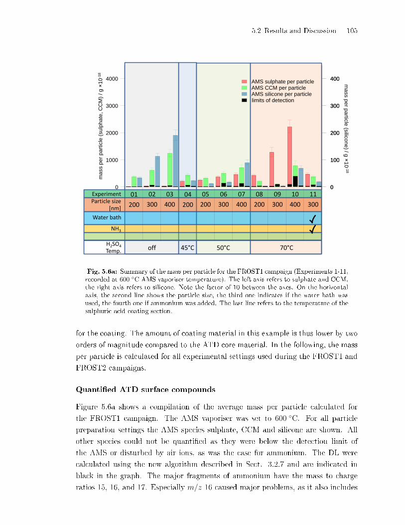
5.2 Results and Discussion 105
Particle size [nm]
NH3
Water bath
H2SO4
Temp.
200 300 400 200 300 400 300 200 200 300 400
off 45°C 50°C 70°C
ma
ss p
er
part
icle
(su
lph
ate
, C
CM
) / g
×10
-18
ma
ss p
er p
artic
le (s
ilico
ne
) / g ×
10
-18
4000
3000
2000
1000
0
400
300
200
100
0
400
300
200
100
0
AMS sulphate per particle AMS CCM per particle AMS silicone per particle limits of detection
Experiment 01 02 03 08 09 10 11 04 05 06 07
Fig. 5.6a: Summary of the mass per particle for the FROST1 campaign (Experiments 1-11,recorded at 600 ◦C AMS vaporiser temperature). The left axis refers to sulphate and CCM,the right axis refers to silicone. Note the factor of 10 between the axes. On the horizontalaxis, the second line shows the particle size, the third one indicates if the water bath wasused, the fourth one if ammonium was added. The last line refers to the temperature of thesulphuric acid coating section.
for the coating. The amount of coating material in this example is thus lower by two
orders of magnitude compared to the ATD core material. In the following, the mass
per particle is calculated for all experimental settings used during the FROST1 and
FROST2 campaigns.
Quanti�ed ATD surface compounds
Figure 5.6a shows a compilation of the average mass per particle calculated for
the FROST1 campaign. The AMS vaporiser was set to 600 ◦C. For all particle
preparation settings the AMS species sulphate, CCM and silicone are shown. All
other species could not be quanti�ed as they were below the detection limit of
the AMS or disturbed by air ions, as was the case for ammonium. The DL were
calculated using the new algorithm described in Sect. 3.2.7 and are indicated in
black in the graph. The major fragments of ammonium have the mass to charge
ratios 15, 16, and 17. Especially m/z 16 caused major problems, as it also includes
106 5 Laboratory Studies on the Ice Nucleation E�ciency of ATD
the O+ ions from the air. The signal of the O+ ions is calculated from the air signal
on m/z 14 (N+) and subtracted from the total signal on m/z 16 in order to obtain
the contribution of the other species. It is assumed that the ratio between nitrogen
and oxygen in the air is constant (Allan et al., 2004). However, this was not the
case during this study. The highest �uctuations of the ratio between oxygen and
nitrogen were observed when ammonia was added to the particle �ow to neutralise
the particles. The ammonia was mixed with nitrogen and its �ow seemed to be
slightly unstable, thus varying the amount of nitrogen added during the experiments.
In the DMA a fraction of this additional nitrogen could di�use into the air that was
sampled by the AMS. The reason for the small �uctuations when no nitrogen was
added are unknown. An alternative to the correction via the nitrogen signal at m/z
14 appeared to be the direct use of the signal on m/z 32, which corresponds to O+2 .
This way the in�uence of the �uctuations of the ratio between the oxygen and the
nitrogen concentration is avoided. However when using this correction in situations
which were known not to contain ammonium, it nevertheless showed �uctuation
around the zero line which were clearly higher than the noise level. Finally it was
only possible to use the ammonium signal for experiments during FROST2 with
the water bath in use and with a sulphuric acid bath temperature of 85 ◦C. These
experiments yielded the thickest coatings of this study. Only for these measurements,
the ammonia uptake was high enough to provide a signal which was clearly above
the �uctuations caused by the nitrogen-oxygen-ratio �uctuations.
Mass per particle during FROST1
The �rst three experiments in Fig. 5.6a show the non-refractory mass loadings for
uncoated ATD particles with mobility diameters of 200 nm, 300 nm, and 400 nm.
The amount of CCM and silicone is proportional to the squared particle diameters
and thus to the particle's surface areas. This indicates that all of the detected
material originates from the particle surface and not from the bulk of the particles.
The next three temperature groups (experiments 04-11) present measurements for
which the particles were coated at 45, 50 and 70 ◦C. As expected, the amount of
sulphate on the particles increases with coating bath temperature as can be seen
for example by comparing experiments 04, 05 and 08 with an identical particle size
of 200 nm. While the sulphate mass per particle for one particle size increased, the
amount of silicone decreased. This can most likely be explained by oxidation of the
methyl silicone by the sulphuric acid. If a complete oxidation occurs, the following
chemical reaction is proposed:
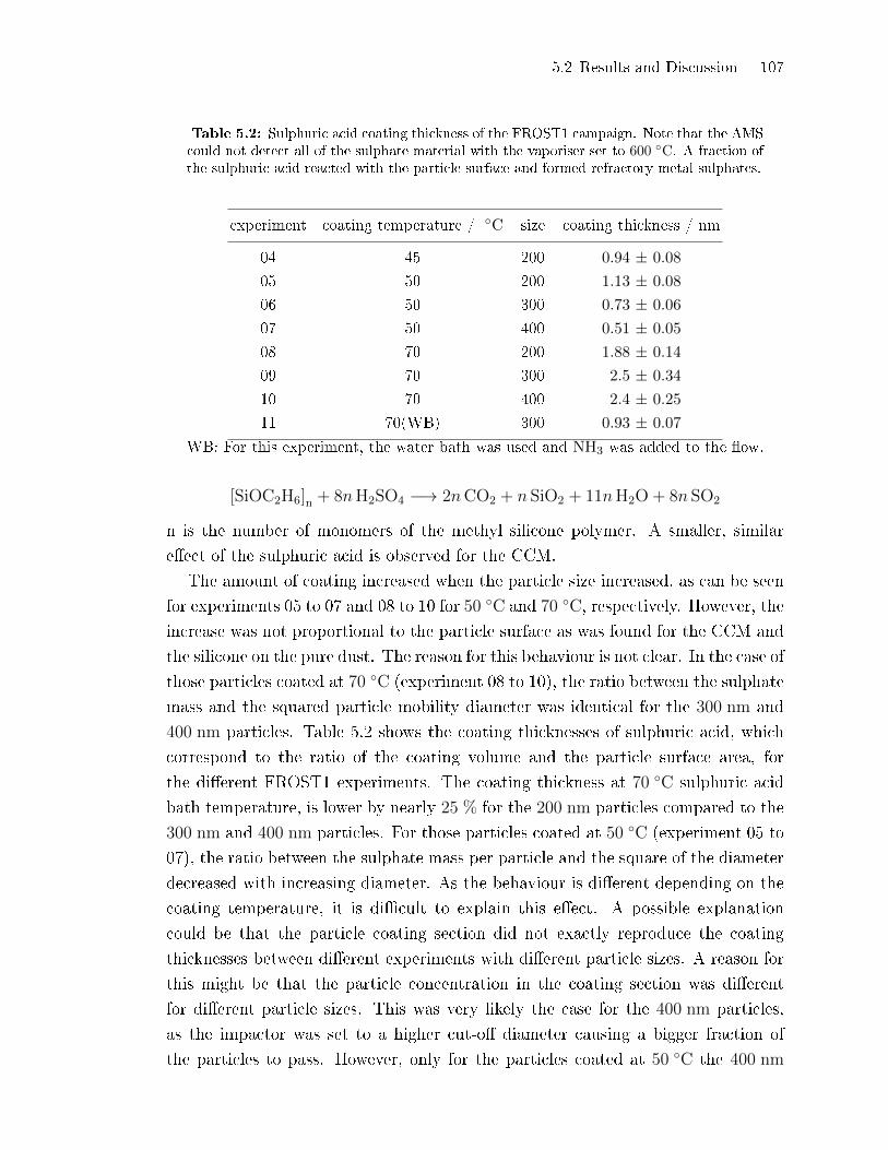
5.2 Results and Discussion 107
Table 5.2: Sulphuric acid coating thickness of the FROST1 campaign. Note that the AMScould not detect all of the sulphate material with the vaporiser set to 600 ◦C. A fraction ofthe sulphuric acid reacted with the particle surface and formed refractory metal sulphates.
experiment coating temperature / ◦C size coating thickness / nm
04
05
06
07
08
09
10
11
45
50
50
50
70
70
70
70(WB)
200
200
300
400
200
300
400
300
0.94 ± 0.08
1.13 ± 0.08
0.73 ± 0.06
0.51 ± 0.05
1.88 ± 0.14
2.5 ± 0.34
2.4 ± 0.25
0.93 ± 0.07
WB: For this experiment, the water bath was used and NH3 was added to the �ow.
[SiOC2H6]n + 8nH2SO4 −→ 2nCO2 + n SiO2 + 11nH2O+ 8n SO2
n is the number of monomers of the methyl silicone polymer. A smaller, similar
e�ect of the sulphuric acid is observed for the CCM.
The amount of coating increased when the particle size increased, as can be seen
for experiments 05 to 07 and 08 to 10 for 50 ◦C and 70 ◦C, respectively. However, the
increase was not proportional to the particle surface as was found for the CCM and
the silicone on the pure dust. The reason for this behaviour is not clear. In the case of
those particles coated at 70 ◦C (experiment 08 to 10), the ratio between the sulphate
mass and the squared particle mobility diameter was identical for the 300 nm and
400 nm particles. Table 5.2 shows the coating thicknesses of sulphuric acid, which
correspond to the ratio of the coating volume and the particle surface area, for
the di�erent FROST1 experiments. The coating thickness at 70 ◦C sulphuric acid
bath temperature, is lower by nearly 25 % for the 200 nm particles compared to the
300 nm and 400 nm particles. For those particles coated at 50 ◦C (experiment 05 to
07), the ratio between the sulphate mass per particle and the square of the diameter
decreased with increasing diameter. As the behaviour is di�erent depending on the
coating temperature, it is di�cult to explain this e�ect. A possible explanation
could be that the particle coating section did not exactly reproduce the coating
thicknesses between di�erent experiments with di�erent particle sizes. A reason for
this might be that the particle concentration in the coating section was di�erent
for di�erent particle sizes. This was very likely the case for the 400 nm particles,
as the impactor was set to a higher cut-o� diameter causing a bigger fraction of
the particles to pass. However, only for the particles coated at 50 ◦C the 400 nm
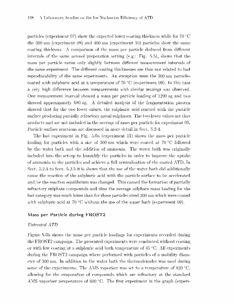
108 5 Laboratory Studies on the Ice Nucleation E�ciency of ATD
particles (experiment 07) show the expected lower coating thickness while for 70 ◦C
the 300 nm (experiment 09) and 400 nm (experiment 10) particles show the same
coating thickness. A comparison of the mass per particle deduced from di�erent
intervals of the same aerosol preperation setting (e.g.: Fig. 5.5), shows that the
mass per particle varies only slightly between di�erent measurement intervals of
the same experiment. The di�erent coating thicknesses are thus not related to bad
reproducability of the same experiments. An exception were the 300 nm particles
coated with sulphuric acid at a temperature of 70 ◦C (experiment 09). In this case
a very high di�erence between measurements with similar settings was observed.
One measurement interval showed a mass per particle loading of 1290 ag and two
showed approximately 680 ag. A detailed analysis of the fragmentation pattern
showed that for the two lower values, the sulphuric acid reacted with the particle
surface producing partially refractory metal sulphates. The two lower values are thus
artefacts and are not included in the average of mass per particle for experiment 09.
Particle surface reactions are discussed in more detail in Sect. 5.2.4.
The last experiment in Fig. 5.6a (experiment 11) shows the mass per particle
loading for particles with a size of 300 nm which were coated at 70 ◦C followed
by the water bath and the addition of ammonia. The water bath was originally
included into the set-up to humidify the particles in order to improve the uptake
of ammonia to the particles and achieve a full neutralisation of the coated ATD. In
Sect. 5.2.3 to Sect. 5.2.5 it is shown that the use of the water bath did additionally
cause the reaction of the sulphuric acid with the particle surface to be accelerated
and/or the reaction equilibrium was changed. This caused the formation of partially
refractory sulphate compounds and thus the average sulphate mass loading for the
last category was much lower than for those particles sized 300 nm which were coated
with sulphuric acid at 70 ◦C without the use of the water bath (experiment 09).
Mass per Particle during FROST2
Untreated ATD
Figure 5.6b shows the mass per particle loadings for experiments recorded during
the FROST2 campaign. The presented experiments were conducted without coating
or with low coating at a sulphuric acid bath temperature of 45 ◦C. All experiments
during the FROST2 campaign where performed with particles of a mobility diam-
eter of 300 nm. In addition to the water bath the thermodenuder was used during
some of the experiments. The AMS vaporiser was set to a temperature of 820 ◦C,
allowing for the evaporation of compounds which are refractory at the standard
AMS vaporiser temperature of 600 ◦C. The �rst experiment in the graph (experi-
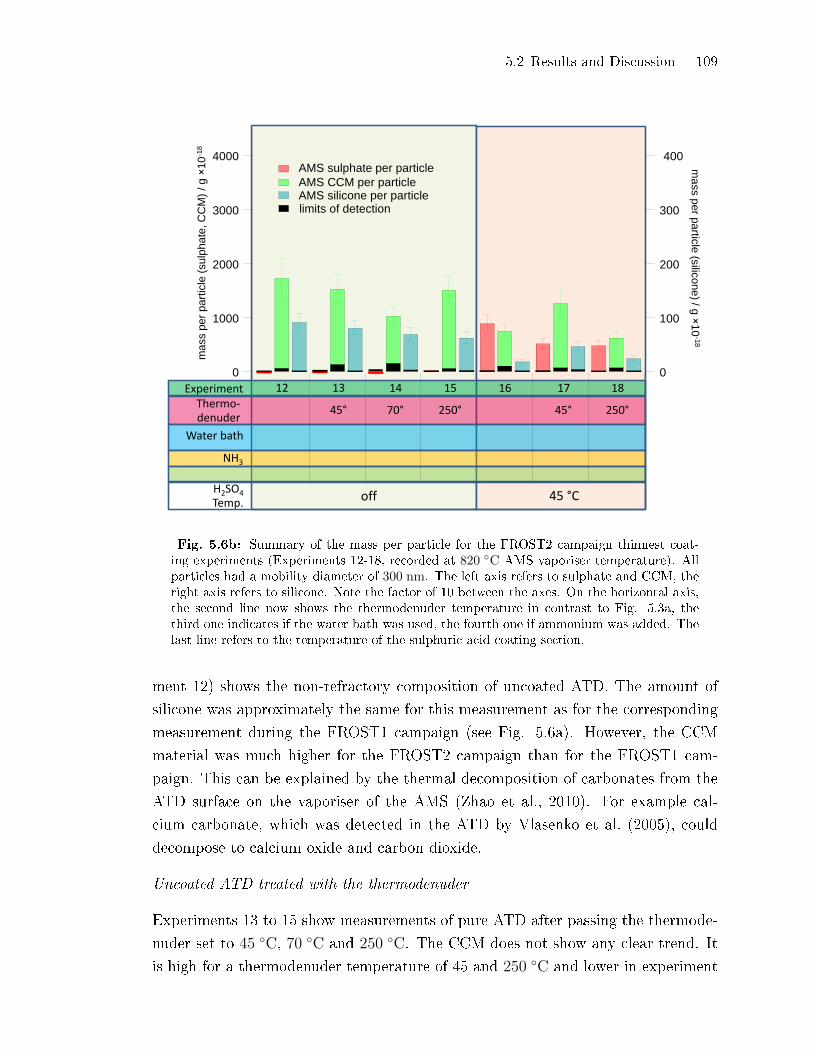
5.2 Results and Discussion 109
Thermo-denuder
off 45 °C
45° 70° 250° 45° 250°
ma
ss p
er
part
icle
(su
lph
ate
, C
CM
) / g
×10
-18
ma
ss p
er p
artic
le (s
ilico
ne
) / g ×
10
-18
4000
3000
2000
1000
0
400
300
200
100
0
AMS sulphate per particle
AMS CCM per particle AMS silicone per particle limits of detection
Experiment 13 14 18 17 15 12 16
NH3
Water bath
H2SO4
Temp.
Fig. 5.6b: Summary of the mass per particle for the FROST2 campaign thinnest coat-ing experiments (Experiments 12-18, recorded at 820 ◦C AMS vaporiser temperature). Allparticles had a mobility diameter of 300 nm. The left axis refers to sulphate and CCM, theright axis refers to silicone. Note the factor of 10 between the axes. On the horizontal axis,the second line now shows the thermodenuder temperature in contrast to Fig. 5.3a, thethird one indicates if the water bath was used, the fourth one if ammonium was added. Thelast line refers to the temperature of the sulphuric acid coating section.
ment 12) shows the non-refractory composition of uncoated ATD. The amount of
silicone was approximately the same for this measurement as for the corresponding
measurement during the FROST1 campaign (see Fig. 5.6a). However, the CCM
material was much higher for the FROST2 campaign than for the FROST1 cam-
paign. This can be explained by the thermal decomposition of carbonates from the
ATD surface on the vaporiser of the AMS (Zhao et al., 2010). For example cal-
cium carbonate, which was detected in the ATD by Vlasenko et al. (2005), could
decompose to calcium oxide and carbon dioxide.
Uncoated ATD treated with the thermodenuder
Experiments 13 to 15 show measurements of pure ATD after passing the thermode-
nuder set to 45 ◦C, 70 ◦C and 250 ◦C. The CCM does not show any clear trend. It
is high for a thermodenuder temperature of 45 and 250 ◦C and lower in experiment
110 5 Laboratory Studies on the Ice Nucleation E�ciency of ATD
14, where the thermodenuder was set to 70 ◦C. The silicone is slightly reduced by
the thermodenuder. It would be surprising if the silicone present on the particle
surface had a volatility which is low enough to remain mainly on the particle surface
even at a denuder temperature of 250 ◦C. It is therefore likely that the main frac-
tion of the silicone was condensing on the particle surface after the aerosol passed
the thermodenuder. This could be explained by the assumption that the silicone is
present in the compressed air rather than being already present on the ATD surface
after the manufacturing of the dust.
ATD coated at 45 ◦C
During experiments 16 to 18 a low amount of sulphuric acid was condensed on
the particle surface with the sulphuric acid coating bath set to 45 ◦C. The coat-
ing thicknesses ranged from 0.95± 0.16 nm (491 ag) to 1.7± 0.3 nm (901 ag). The
�rst of these three experiments shows the e�ect of condensing sulphuric acid on the
ATD without further processing. Similar to the FROST1 data, the silicone was
clearly reduced by the addition of sulphuric acid which reacted with the silicone.
The sulphuric acid could consume silicone present on the particle surface or silicone
which was condensing on the ATD after the sulphuric acid coating. In experiment
17 and 18, the e�ect of the thermodenuder on the amount of sulphate was anal-
ysed. The denuder was set to temperatures of 45 ◦C and 250 ◦C, respectively. The
thermodenuder originally was meant to remove the sulphuric acid from the particle
surface in order to check if the IN-e�ciency of ATD could be restored this way.
However, the graph shows that most of the sulphate signal that was present on the
non-denuded particles, remained after the denuding. The reason for this is that the
thermodenuder, similar to the water bath, accelerates the reactions with the particle
surface, resulting in compounds with lower volatility which cannot be removed by
the thermodenuder. More details are presented in Sect. 5.2.4. Interestingly, the
silicone signal is higher when the thermodenuder is used compared to experiment
16 which was conducted without the thermodenuder. The highest silicone signal for
the coated particles was observed at a thermodenuder temperature of 45 ◦C. This
favours the assumption that the silicone was at least partially condensed on the
ATD after the particle generation section. After applying the thermodenuder, no
unreacted sulphuric acid was left on the particle surface to oxidise newly condensing
silicone.
ATD coated at 70 ◦C without further processing
Figure 5.6c shows the mass per particle loadings for those particles which were
coated by medium and thick coatings, corresponding to coating bath temperatures
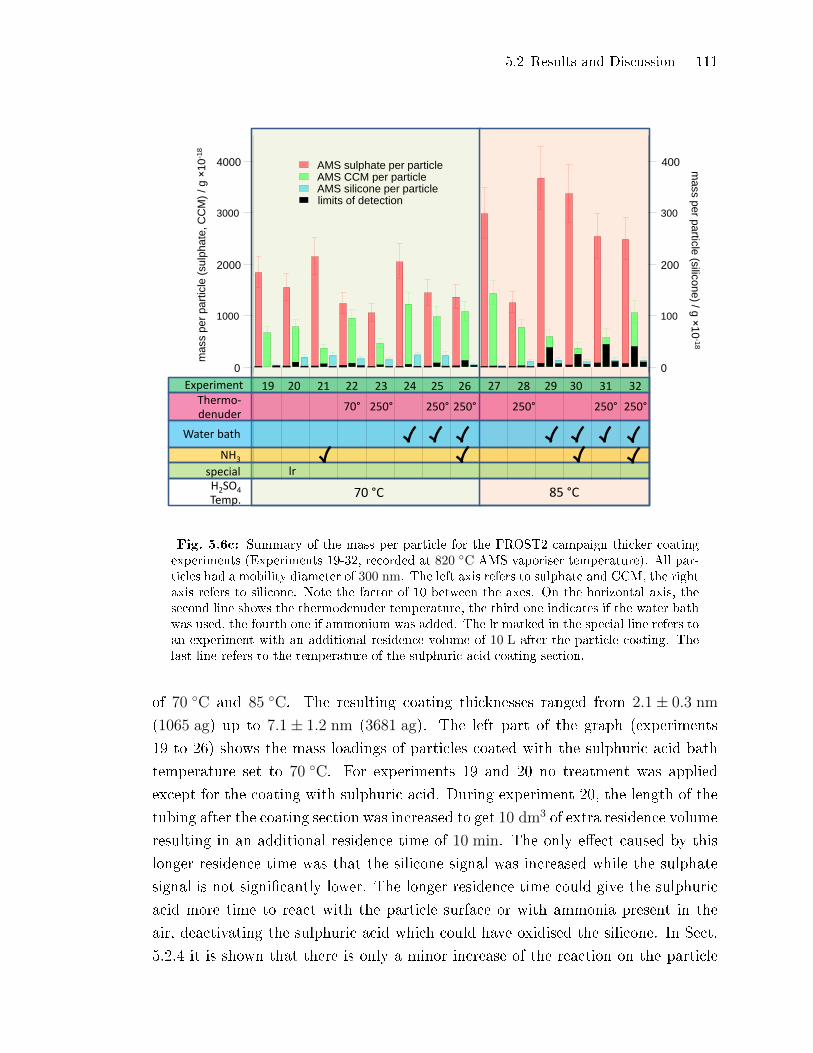
5.2 Results and Discussion 111
Thermo-denuder
NH3
special
Water bath
70 °C 85 °C H2SO4
Temp.
4000
3000
2000
1000
0
400
300
200
100
0
AMS sulphate per particle AMS CCM per particle AMS silicone per particle limits of detection
70°
lr
250° 250° 250° 250° 250° 250°
ma
ss p
er
pa
rtic
le (
su
lph
ate
, C
CM
) / g
×10
-18
ma
ss p
er p
artic
le (s
ilico
ne
) / g ×
10
-18
Experiment 22 23 32 31 28 26 25 20 21 19 24 29 30 27
Fig. 5.6c: Summary of the mass per particle for the FROST2 campaign thicker coatingexperiments (Experiments 19-32, recorded at 820 ◦C AMS vaporiser temperature). All par-ticles had a mobility diameter of 300 nm. The left axis refers to sulphate and CCM, the rightaxis refers to silicone. Note the factor of 10 between the axes. On the horizontal axis, thesecond line shows the thermodenuder temperature, the third one indicates if the water bathwas used, the fourth one if ammonium was added. The lr marked in the special line refers toan experiment with an additional residence volume of 10 L after the particle coating. Thelast line refers to the temperature of the sulphuric acid coating section.
of 70 ◦C and 85 ◦C. The resulting coating thicknesses ranged from 2.1± 0.3 nm
(1065 ag) up to 7.1± 1.2 nm (3681 ag). The left part of the graph (experiments
19 to 26) shows the mass loadings of particles coated with the sulphuric acid bath
temperature set to 70 ◦C. For experiments 19 and 20 no treatment was applied
except for the coating with sulphuric acid. During experiment 20, the length of the
tubing after the coating section was increased to get 10 dm3 of extra residence volume
resulting in an additional residence time of 10 min. The only e�ect caused by this
longer residence time was that the silicone signal was increased while the sulphate
signal is not signi�cantly lower. The longer residence time could give the sulphuric
acid more time to react with the particle surface or with ammonia present in the
air, deactivating the sulphuric acid which could have oxidised the silicone. In Sect.
5.2.4 it is shown that there is only a minor increase of the reaction on the particle

112 5 Laboratory Studies on the Ice Nucleation E�ciency of ATD
surface for the longer residence experiment. Furthermore Sect. 5.2.5 indicates that
particle surface reactions did not result in the formation of refractory substances at
820 ◦C vaporiser temperature. The second possible e�ect, which is the reaction with
the ammonia present in the air is thus more likely. This assumption is supported by
the increase of the ammonium signal for these experiments. However, as mentioned
before, the ammonium signal is disturbed and consequently the observed increase
of ammonium might be an artefact.
E�ect of the water bath and the thermodenuder on particles coated with sulphuric
acid at 70 ◦C
The addition of ammonia to the dry, coated ATD (experiment 21) results in a higher
sulphate signal. The signal is slightly higher than for the non-neutralised particles
but the di�erence is not signi�cant. A clear reduction of the sulphate signal can
however be seen for experiments 22, 23, 25 and 26 with the thermodenuder in use.
Even a denuder temperature of 70 ◦C is enough to achieve a reduction of the sulphate
signal in the same range as with the higher temperature of 250 ◦C. The use of the
water bath prior to the thermodenuder (experiments 25 and 26) resulted in a slightly
higher signal for the sulphate. The use of the water bath without the thermodenuder
again results in a similar sulphate mass per particle as found when only coating the
particles.
E�ect of the thermodenuder with and without prior humidi�cation of the ATD
coated at 85 ◦C
On the right side of Fig. 5.6c (experiments 27 to 32) particles coated with the
sulphuric acid bath set to 85 ◦C are shown. Qualitatively the same e�ects can
be seen as for those experiments with thinner coatings for which the coating bath
temperature was adjusted to 70 ◦C. However, the di�erence in the sulphate mass per
particle between those particles which were denuded without prior humidi�cation
(experiment 28) and those that passed the water bath before the thermodenuder
(experiments 31 and 32) is much clearer. This can be explained by the observation
(Sect. 5.2.4) that the water bath accelerated reactions of the particle surface with
the sulphuric acid, producing products which cannot be easily evaporated by the
thermodenuder. This interpretation is also in accordance with the higher di�erence
between the denuded and humidi�ed particles (experiment 31 and 32) and those
that were only denuded (experiment 28), when comparing the thicker coatings to
the medium coatings (experiments 22 to 26). When the thermodenuder was used
without prior humidi�cation of the particles, more time is necessary for the thicker

5.2 Results and Discussion 113
coatings to completely react with the particle surface. Consequently more unreacted
sulphuric acid was left on these particles, which could be evaporated at 250 ◦C.
Detection of ammonium on the ATD particles coated at 85 ◦C
For those particles which were coated at a temperature of 85 ◦C and processed with
the water bath (experiements 29 and 30) the ammonium signal was high enough
to be quanti�ed. The ammonium measured for these experiments corresponds to
0.51± 0.12 times the concentration necessary for a complete neutralisation of the
sulphuric acid. This value was calculated by dividing the ammonium mass per par-
ticle by the amount of ammonium necessary to completely neutralise the sulphuric
acid. The amount of ammonium per particle was calculated i the same way as the
sulphate mass per particle. The uncertainty was calculated using Gaussian error
propagation. However, when the thermodenuder was used after the water bath, the
ammonium signal was reduced at least by a factor of 2.
Silicone: A useful contaminant
The silicone was present for all categories except when no more processing than
coating with sulphuric acid was performed. This matches the assumption that the
silicone condensed on the particles after the processing section because all process-
ings led at least to a partial consumption of the sulphuric acid. A longer residence
time could also lead to a partial neutralisation of the sulphuric acid as was indicated
by the ammonium signal. Thus the unreacted sulphuric acid would also be reduced
for experiment 20. This indicates that the elevated ammonium signal for the longer
residence is not an artefact. Silicone could only survive on the ATD surface, when
the reactivity of the sulphate compounds was reduced. The silicone contamination
can therefore be used as a possible proxy for the presence of unreacted sulphuric
acid after the particle preparation section.
Generally, the sulphate mass per particle loadings for the di�erent processes show
that the sulphuric acid did not only produce a coating on the surface of the ATD
but it also reacted with the surface. In the following, stronger evidence for surface
reactions is provided and linked to the reduction of the ATD IN-e�ciency when
subject to sulphuric acid coating.
5.2.3 Comparison of AMS Sulphate Concentrations to the IN-E�ciency
of ATD
In this section, the sulphate mass per particle is compared to the IN-fraction calcu-
lated from the CFDC data and the LACIS data. For all experiments shown in this
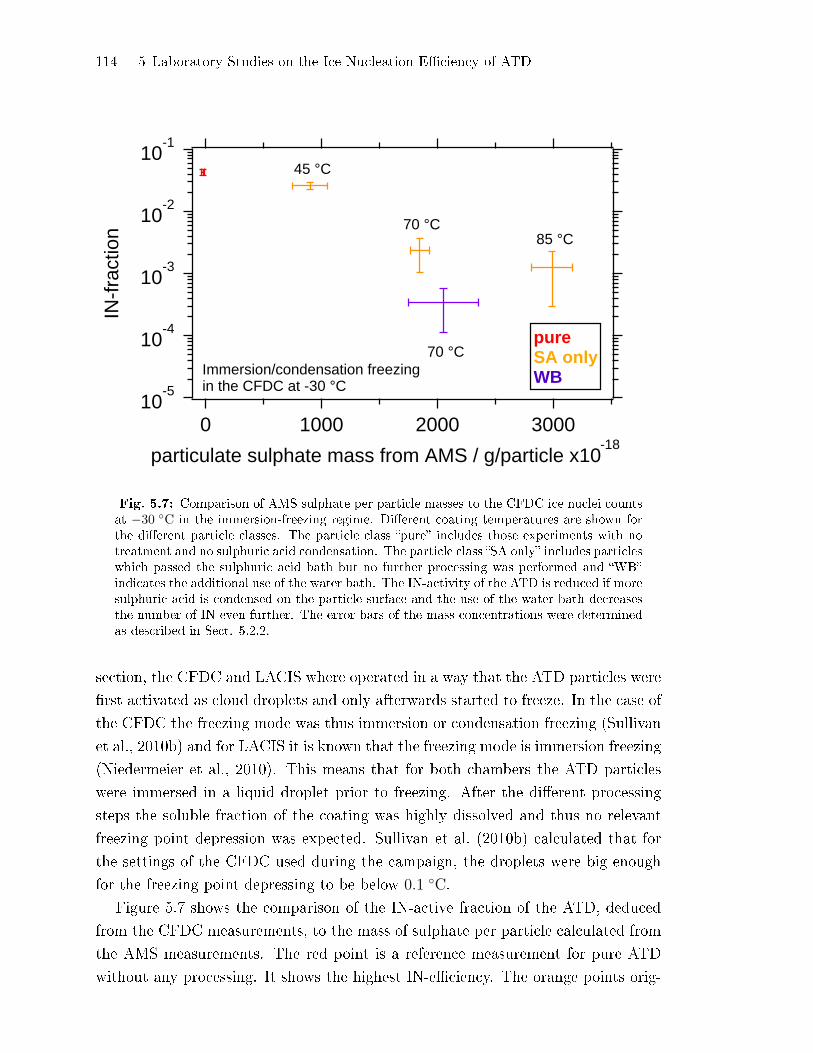
114 5 Laboratory Studies on the Ice Nucleation E�ciency of ATD
10-5
10-4
10-3
10-2
10-1
IN-f
ract
ion
3000200010000
particulate sulphate mass from AMS / g/particle x10-18
Immersion/condensation freezingin the CFDC at -30 °C
70 °C85 °C
70 °C
45 °C
pureSA onlyWB
Fig. 5.7: Comparison of AMS sulphate per particle masses to the CFDC ice nuclei countsat −30 ◦C in the immersion-freezing regime. Di�erent coating temperatures are shown forthe di�erent particle classes. The particle class �pure� includes those experiments with notreatment and no sulphuric acid condensation. The particle class �SA only� includes particleswhich passed the sulphuric acid bath but no further processing was performed and �WB�indicates the additional use of the water bath. The IN-activity of the ATD is reduced if moresulphuric acid is condensed on the particle surface and the use of the water bath decreasesthe number of IN even further. The error bars of the mass concentrations were determinedas described in Sect. 5.2.2.
section, the CFDC and LACIS where operated in a way that the ATD particles were
�rst activated as cloud droplets and only afterwards started to freeze. In the case of
the CFDC the freezing mode was thus immersion or condensation freezing (Sullivan
et al., 2010b) and for LACIS it is known that the freezing mode is immersion freezing
(Niedermeier et al., 2010). This means that for both chambers the ATD particles
were immersed in a liquid droplet prior to freezing. After the di�erent processing
steps the soluble fraction of the coating was highly dissolved and thus no relevant
freezing point depression was expected. Sullivan et al. (2010b) calculated that for
the settings of the CFDC used during the campaign, the droplets were big enough
for the freezing point depressing to be below 0.1 ◦C.
Figure 5.7 shows the comparison of the IN-active fraction of the ATD, deduced
from the CFDC measurements, to the mass of sulphate per particle calculated from
the AMS measurements. The red point is a reference measurement for pure ATD
without any processing. It shows the highest IN-e�ciency. The orange points orig-
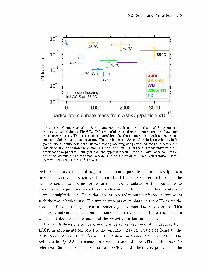
5.2 Results and Discussion 115
10-5
10-4
10-3
10-2
10-1
IN-f
ract
ion
3000200010000
particulate sulphate mass from AMS / g/particle x10-18
pureSA onlyWBWB & TDTD
70 °C
85 °C
45 °C
85 °C
70 °C
70 °C
Immersion freezingin LACIS at -35 °C
45 °C
Fig. 5.8: Comparison of AMS sulphate per particle masses to the LACIS ice nucleuscounts at −35 ◦C during FROST2. Di�erent sulphuric acid bath temperatures are shown forevery particle class. The particle class �pure� includes those experiments with no treatmentand no sulphuric acid condensation. The particle class �SA only� includes particles whichpassed the sulphuric acid bath but no further processing was performed. �WB� indicates theadditional use of the water bath and �TD� the additional use of the thermodenuder after thetreatment except for the blue point on the upper left which refers to particles which passedthe thermodenuder but were not coated. The error bars of the mass concentrations weredetermined as described in Sect. 5.2.2.
inate from measurements of sulphuric acid coated particles. The more sulphate is
present on the particles' surface the more the IN-e�ciency is reduced. Again, the
sulphate signal must be interpreted as the sum of all substances that contribute to
the mass to charge ratios related to sulphate compounds which include sulphate salts
as well as sulphuric acid. Those data points coloured in purple refer to measurements
with the water bath in use. For similar amounts of sulphate on the ATD as for the
non-humidi�ed particles, these measurements yielded much lower IN-fractions. This
is a strong indication that humidi�cation enhances reactions on the particle surface
which contribute to the reduction of the ice active surface properties.
Figure 5.8 shows the comparison of the ice active fraction of ATD deduced from
LACIS measurements compared to the sulphate mass per particle as found by the
AMS. A comparison of LACIS and CFDC is shown in Niedermeier et al. (2011). The
red point in Fig. 5.8 corresponds to a measurement of pure ATD and is shown for
reference. Similar to the comparison to the CFDC data the orange points show the

116 5 Laboratory Studies on the Ice Nucleation E�ciency of ATD
e�ect of coating with sulphuric acid without further processing, which also resulted
in a reduction of the ice active fraction of the ATD. The water bath data, marked in
purple, show the same e�ect as in the comparison with the CFDC: the IN-fraction
is further reduced. For the comparison of the LACIS data with the AMS sulphate
mass fraction, data with the thermodenuder in use were available. Those data
points which refer to measurements with the thermodenuder used after the coating
and the water bath are coloured in green. They show the same IN-fraction for a
given sulphate mass per particle as those data points which refer to coated particles
which were only humidi�ed after the coating. This indicates that after the use of
the water bath, nearly no sulphuric acid is left, as sulphuric acid would be removed
from the surface at a thermodenuder temperature of 250 ◦C.
The blue points in Fig. 5.8 mark those experiments which a thermodenuder
temperature of 250 ◦C but without prior use of the water bath. The blue point
close to the red point was recorded without coating and is used as reference. This
point shows that the heating in the thermodenuder alone is not able to reduce the
IN-fraction of the ATD. However, when the particles were coated prior to passing
the thermodenuder, the IN-fraction is strongly reduced. It appears as if the e�ect
was even stronger than for the water bath only, but it has to be considered that
the thermodenuder also removes part of the sulphuric acid and thus shifts the blue
points to the left. Therefore, the heat processing e�ect of the thermodenuder when
used after the sulphuric acid coating can be considered to be similar to the e�ect of
the water bath.
In Sullivan et al. (2010b) the strong reduction of the IN-fraction due to the use
of the water bath after the sulphuric acid coating was interpreted as an irreversible
destruction of ice active sites. The destruction is thought to be irreversible because
the particles had been activated as cloud droplets when the freezing occurred. If
the sulphuric acid acted as a pure surface covering e�ect, the activation as a water
droplet would have dissolved the sulphuric acid. Thus, the IN-ability of the ATD
should have been restored as the freezing point depression e�ect was negligible. The
fact that the IN-e�ciency was not restored after the droplet activation is thus a
further indication for a reaction on the particle surface which can not be reversed.
The nature of the active sites is still unknown, but it appears that they can be
destroyed by etching through sulphuric acid. A possible property of ice active sites
could be a structure which is similar to hexagonal ice and which can participate in
hydrogen bond like interactions (Pruppacher and Klett, 1997, chapter 9.2) or related
to strong local electric �elds, as was indicated by Choi et al. (2005). Cubic ice for-
mation appears to be relevant in homogeneous freezing (Murray and Bertram, 2006,
5.2 Results and Discussion 117
Murray et al., 2005). Therefore it could be expected that cubic-ice-like-structures
might also play a role in heterogeneous ice formation (Eastwood et al., 2008). Other
properties are also possible. The properties which are crucial for the ATD to act
as an ice nucleus cannot be fully explained in this study. However, the possible
chemical nature of active sites can be analysed.
5.2.4 Sulphate Fragmentation Pattern: Evidence for ATD Surface
Etching
In the preceding sections, it became clear that a reaction of the sulphuric acid with
the particle surface is probably taking place but could not be detected directly. In
this section, evidence for a reaction of the sulphuric acid with the particle surface
is given by showing that after the use of the water bath and/or the thermodenuder,
the compounds belonging to the AMS sulphate species are no longer sulphuric acid
but must be metal sulphates. First possible reactions are suggested and afterwards
they are experimentally veri�ed.
The following model reactions (React. (R5.1) to React. (R5.7)) are suggested
to take place on the particle surface, based on the available material. M is a metal
with a valency of 3 e.g. aluminium. However, other metals which are present on
the ATD surface with di�erent valencies were probabely also involved in the surface
reactions. Carbonate is shown as an example for an anion. In Sect. 5.2.5 an analysis
is presented to �nd out which metals were involved in the surface reactions and the
possible anions are discussed. The reaction equations are not equilibrated as the
relative contribution of the di�erent products is unknown.
Reaction (R5.1) refers to a coating with sulphuric acid followed by a humidi�ca-
tion of the particle surface by the water bath. Beside the metal sulphates, mixed
sulphates of ammonium and a metal are also possible. Part of the sulphuric acid is
also expected to be neutralised to ammonium sulphate. Water and carbondioxide
can form in this process and are released to the gas phase as indicated by �g�. Re-
action (R5.2) describes the evaporation of the compounds formed in React. (R5.1)
on the AMS vaporiser. Only those compounds marked with �g� were evaporated
and could be detected in the AMS. SOi with i equal to 1, 2 or 3 as well as H2SO4
contributed to the AMS sulphate species signal. H2O is veiled by the instrument
residual gas and NH3 contributes to the ammonium species signal. However, as
mentioned in Sect. 5.2.2, most of the time it was not possible to quantify ammo-
nium.
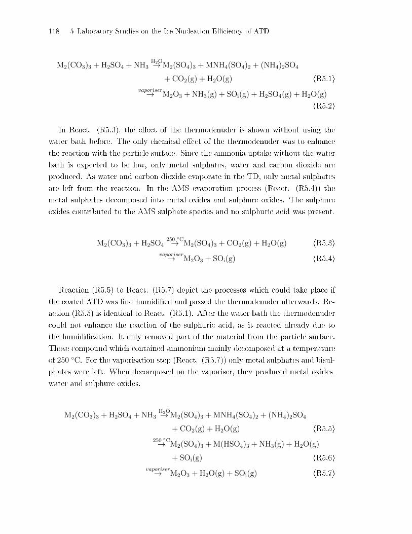
118 5 Laboratory Studies on the Ice Nucleation E�ciency of ATD
M2(CO3)3 +H2SO4 +NH3H2O→M2(SO4)3 +MNH4(SO4)2 + (NH4)2SO4
+ CO2(g) + H2O(g) (R5.1)
vaporiser→ M2O3 +NH3(g) + SOi(g) + H2SO4(g) + H2O(g)
(R5.2)
In React. (R5.3), the e�ect of the thermodenuder is shown without using the
water bath before. The only chemical e�ect of the thermodenuder was to enhance
the reaction with the particle surface. Since the ammonia uptake without the water
bath is expected to be low, only metal sulphates, water and carbon dioxide are
produced. As water and carbon dioxide evaporate in the TD, only metal sulphates
are left from the reaction. In the AMS evaporation process (React. (R5.4)) the
metal sulphates decomposed into metal oxides and sulphure oxides. The sulphure
oxides contributed to the AMS sulphate species and no sulphuric acid was present.
M2(CO3)3 +H2SO4250 ◦C→ M2(SO4)3 + CO2(g) + H2O(g) (R5.3)
vaporiser→ M2O3 + SOi(g) (R5.4)
Reaction (R5.5) to React. (R5.7) depict the processes which could take place if
the coated ATD was �rst humidi�ed and passed the thermodenuder afterwards. Re-
action (R5.5) is identical to React. (R5.1). After the water bath the thermodenuder
could not enhance the reaction of the sulphuric acid, as it reacted already due to
the humidi�cation. It only removed part of the material from the particle surface.
Those compound which contained ammonium mainly decomposed at a temperature
of 250 ◦C. For the vaporisation step (React. (R5.7)) only metal sulphates and bisul-
phates were left. When decomposed on the vaporiser, they produced metal oxides,
water and sulphure oxides.
M2(CO3)3 +H2SO4 +NH3H2O→M2(SO4)3 +MNH4(SO4)2 + (NH4)2SO4
+ CO2(g) + H2O(g) (R5.5)
250 ◦C→ M2(SO4)3 +M(HSO4)3 +NH3(g) + H2O(g)
+ SOi(g) (R5.6)
vaporiser→ M2O3 +H2O(g) + SOi(g) (R5.7)
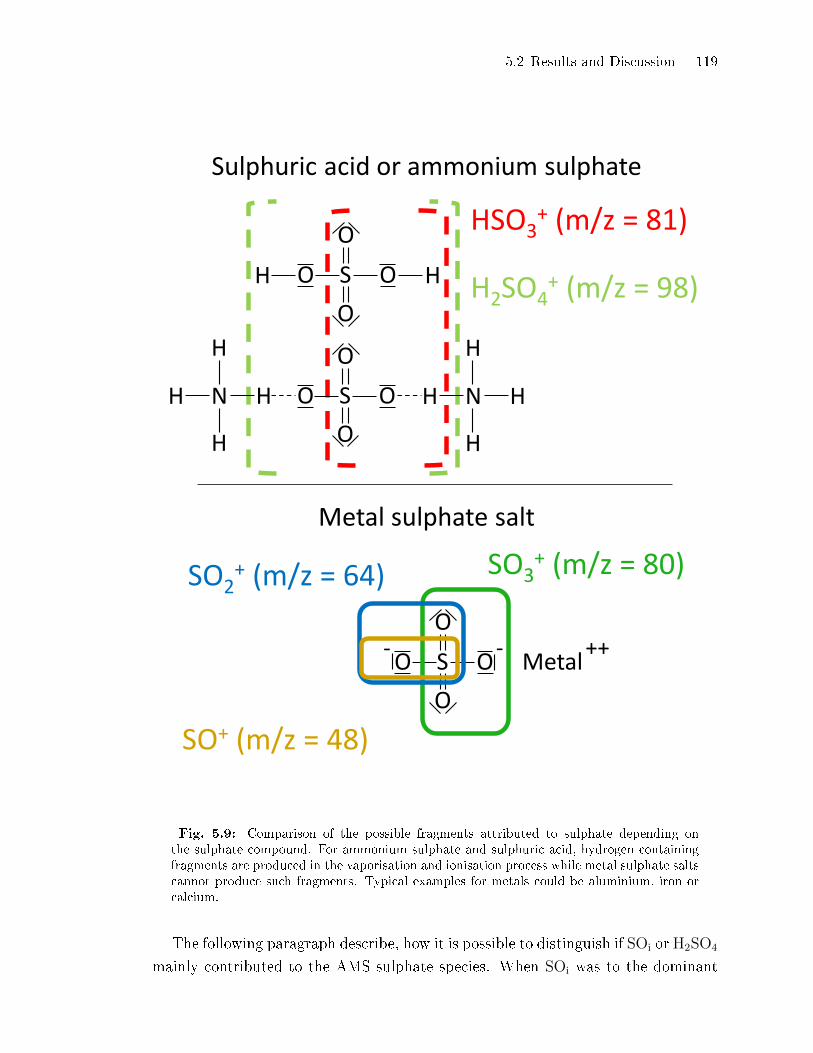
5.2 Results and Discussion 119
S O
O
O
O Metal
HSO3+ (m/z = 81)
S O
O
O
O HH
S O
O
O
O H N H
H
H
H N H
H
H
H2SO4+ (m/z = 98)
SO3+ (m/z = 80) SO2
+ (m/z = 64)
SO+ (m/z = 48)
Sulphuric acid or ammonium sulphate
Metal sulphate salt
SO
O O
OM
etal
SO
O O
OM
etal
- - ++
Fig. 5.9: Comparison of the possible fragments attributed to sulphate depending onthe sulphate compound. For ammonium sulphate and sulphuric acid, hydrogen containingfragments are produced in the vaporisation and ionisation process while metal sulphate saltscannot produce such fragments. Typical examples for metals could be aluminium, iron orcalcium.
The following paragraph describe, how it is possible to distinguish if SOi or H2SO4
mainly contributed to the AMS sulphate species. When SOi was to the dominant
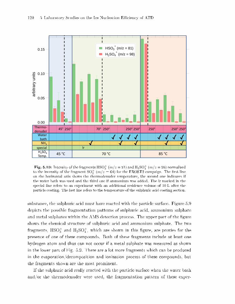
120 5 Laboratory Studies on the Ice Nucleation E�ciency of ATD
0.15
0.10
0.05
0.00
arb
itra
ry u
nits
Thermo-denuder
NH3
special
45° 70°
lr
Water bath
HSO 3
+ (m/z = 81)
H 2 SO 4
+ (m/z = 98)
250° 250° 250° 250° 250° 250° 250°
45 °C 70 °C 85 °C H2SO4
Temp.
Fig. 5.10: Intensity of the fragments HSO+3 (m/z = 81) and H2SO
+4 (m/z = 98) normalised
to the intensity of the fragment SO+2 (m/z = 64) for the FROST2 campaign. The �rst line
on the horizontal axis shows the thermodenuder temperature, the second one indicates ifthe water bath was used and the third one if ammonium was added. The lr marked in thespecial line refers to an experiment with an additional residence volume of 10 L after theparticle coating. The last line refers to the temperature of the sulphuric acid coating section.
substance, the sulphuric acid must have reacted with the particle surface. Figure 5.9
depicts the possible fragmentation patterns of sulphuric acid, ammonium sulphate
and metal sulphates within the AMS detection process. The upper part of the �gure
shows the chemical structure of sulphuric acid and ammonium sulphate. The two
fragments, HSO+3 and H2SO
+4 , which are shown in this �gure, are proxies for the
presence of one of these compounds. Both of these fragments include at least one
hydrogen atom and thus can not occur if a metal sulphate was measured as shown
in the lower part of Fig. 5.9. There are a lot more fragments which can be produced
in the evaporation/decomposition and ionisation process of these compounds, but
the fragments shown are the most prominent.
If the sulphuric acid really reacted with the particle surface when the water bath
and/or the thermodenuder were used, the fragmentation pattern of these exper-

5.2 Results and Discussion 121
iments should show clearly reduced signals at the fragments HSO+3 and H2SO
+4 .
Figure 5.10 shows these fragments for those experiments of the FROST2 campaign,
for which the ATD was coated with sulphuric acid. The �rst three categories with
the blue background refer to a sulphuric acid bath temperature of 45 ◦C. The cat-
egories with the green and the red background refer to coating temperatures of
70 ◦C and 85 ◦C respectively. The categories on the left of the dashed line of each
coating temperature area correspond to measurements for which the particles were
only coated with sulphuric acid and the thermodenuder was not used at a higher
temperature as was used for the coating itself. No water bath was used in these
experiments but ammonia was added to the dry particles for one experiment. On
the right side of the dashed lines, those experiments for which the water bath and/or
the thermodenuder were used after the coating are shown.
For all coating temperatures the intensity of the hydrogen-containing fragments
was clearly reduced when the water bath and/or the thermodenuder were used. This
is in accordance to what could be expected when comparing to the previous section,
where these experiments also showed the highest reduction of the IN-active fraction.
The intensity of the hydrogenated fragments was highest when the coating was
thickest. This also supports the assumption that the sulphuric acid reacted with
the particle surface and that humidi�cation and heating of the particles accelerate
these reactions. For the thin coatings, a higher fraction of the sulphuric acid could
react in the same time compared to thicker coatings, where more sulphuric acid
needed to be consumed. In the case of the thick coatings it was also important to
consider the partial neutralisation of the aerosol due to the omnipresent ammonia.
The neutralisation of parts of the sulphuric acid prior to reaction with the particle
surface led to the formation of ammonium sulphate or bisulphate. These compounds
also produce hydrogenated fragments as has been shown in Fig. 5.9. After neutral-
isation, the sulphuric acid could no longer etch the particle surface. The last two
experimental settings shown in Fig. 5.10 refer to particles which were humidi�ed
before they passed the thermodenuder. Interestingly, these experiments showed no
fragments on m/z 98 but nevertheless a clear signal on m/z 81. It is expected that
the m/z 81 fragments originate from metal bisulphates which produced HSO3 in the
�ash vaporisation process (React. (R5.7)). This is in accordance the the suggested
production of ammonium metal sulphates which decompose to bisulphates in the
TD.
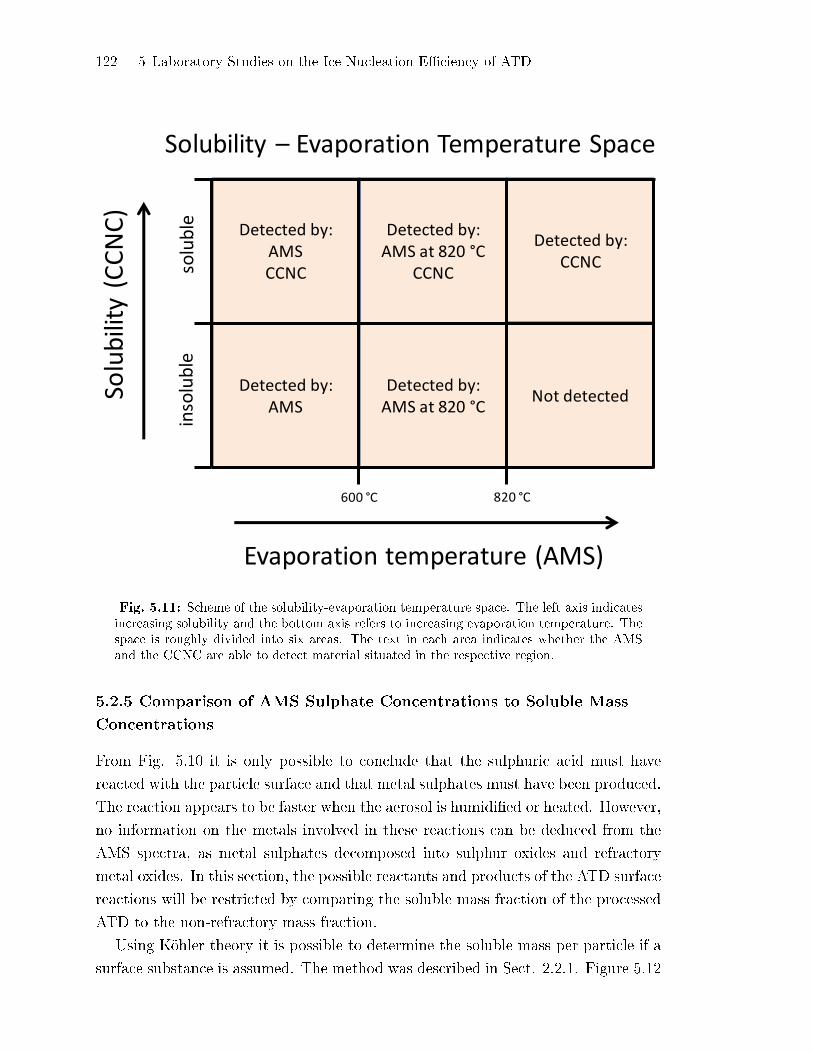
122 5 Laboratory Studies on the Ice Nucleation E�ciency of ATD
Detected by: AMS
Solu
bili
ty (
CC
NC
)
Evaporation temperature (AMS)
600 °C 820 °C
inso
lub
le
solu
ble
Solubility – Evaporation Temperature Space
Detected by: AMS at 820 °C
CCNC
Detected by: AMS at 820 °C
Detected by: CCNC
Detected by: AMS CCNC
Not detected
Fig. 5.11: Scheme of the solubility-evaporation temperature space. The left axis indicatesincreasing solubility and the bottom axis refers to increasing evaporation temperature. Thespace is roughly divided into six areas. The text in each area indicates whether the AMSand the CCNC are able to detect material situated in the respective region.
5.2.5 Comparison of AMS Sulphate Concentrations to Soluble Mass
Concentrations
From Fig. 5.10 it is only possible to conclude that the sulphuric acid must have
reacted with the particle surface and that metal sulphates must have been produced.
The reaction appears to be faster when the aerosol is humidi�ed or heated. However,
no information on the metals involved in these reactions can be deduced from the
AMS spectra, as metal sulphates decomposed into sulphur oxides and refractory
metal oxides. In this section, the possible reactants and products of the ATD surface
reactions will be restricted by comparing the soluble mass fraction of the processed
ATD to the non-refractory mass fraction.
Using Köhler theory it is possible to determine the soluble mass per particle if a
surface substance is assumed. The method was described in Sect. 2.2.1. Figure 5.12
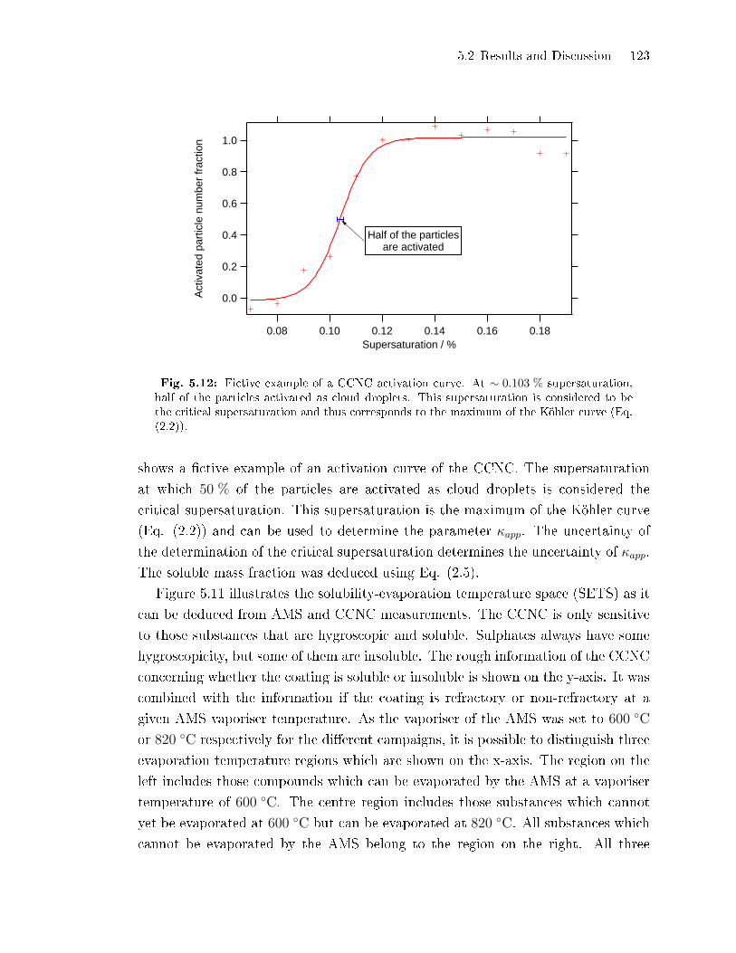
5.2 Results and Discussion 123
1.0
0.8
0.6
0.4
0.2
0.0Act
ivat
ed p
artic
le n
umbe
r fr
actio
n
0.180.160.140.120.100.08Supersaturation / %
Half of the particlesare activated
Fig. 5.12: Fictive example of a CCNC activation curve. At ∼ 0.103 % supersaturation,half of the particles activated as cloud droplets. This supersaturation is considered to bethe critical supersaturation and thus corresponds to the maximum of the Köhler curve (Eq.(2.2)).
shows a �ctive example of an activation curve of the CCNC. The supersaturation
at which 50 % of the particles are activated as cloud droplets is considered the
critical supersaturation. This supersaturation is the maximum of the Köhler curve
(Eq. (2.2)) and can be used to determine the parameter κapp. The uncertainty of
the determination of the critical supersaturation determines the uncertainty of κapp.
The soluble mass fraction was deduced using Eq. (2.5).
Figure 5.11 illustrates the solubility-evaporation temperature space (SETS) as it
can be deduced from AMS and CCNC measurements. The CCNC is only sensitive
to those substances that are hygroscopic and soluble. Sulphates always have some
hygroscopicity, but some of them are insoluble. The rough information of the CCNC
concerning whether the coating is soluble or insoluble is shown on the y-axis. It was
combined with the information if the coating is refractory or non-refractory at a
given AMS vaporiser temperature. As the vaporiser of the AMS was set to 600 ◦C
or 820 ◦C respectively for the di�erent campaigns, it is possible to distinguish three
evaporation temperature regions which are shown on the x-axis. The region on the
left includes those compounds which can be evaporated by the AMS at a vaporiser
temperature of 600 ◦C. The centre region includes those substances which cannot
yet be evaporated at 600 ◦C but can be evaporated at 820 ◦C. All substances which
cannot be evaporated by the AMS belong to the region on the right. All three
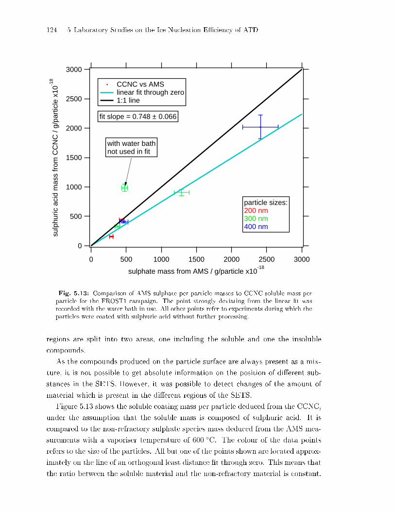
124 5 Laboratory Studies on the Ice Nucleation E�ciency of ATD
3000
2500
2000
1500
1000
500
0
sulp
huric
aci
d m
ass
from
CC
NC
/ g/
part
icle
x10
-18
300025002000150010005000
sulphate mass from AMS / g/particle x10-18
particle sizes:200 nm300 nm400 nm
fit slope = 0.748 ± 0.066
with water bathnot used in fit
CCNC vs AMS linear fit through zero 1:1 line
Fig. 5.13: Comparison of AMS sulphate per particle masses to CCNC soluble mass perparticle for the FROST1 campaign. The point strongly deviating from the linear �t wasrecorded with the water bath in use. All other points refer to experiments during which theparticles were coated with sulphuric acid without further processing.
regions are split into two areas, one including the soluble and one the insoluble
compounds.
As the compounds produced on the particle surface are always present as a mix-
ture, it is not possible to get absolute information on the position of di�erent sub-
stances in the SETS. However, it was possible to detect changes of the amount of
material which is present in the di�erent regions of the SETS.
Figure 5.13 shows the soluble coating mass per particle deduced from the CCNC,
under the assumption that the soluble mass is composed of sulphuric acid. It is
compared to the non-refractory sulphate species mass deduced from the AMS mea-
surements with a vaporiser temperature of 600 ◦C. The colour of the data points
refers to the size of the particles. All but one of the points shown are located approx-
imately on the line of an orthogonal least distance �t through zero. This means that
the ratio between the soluble material and the non-refractory material is constant.
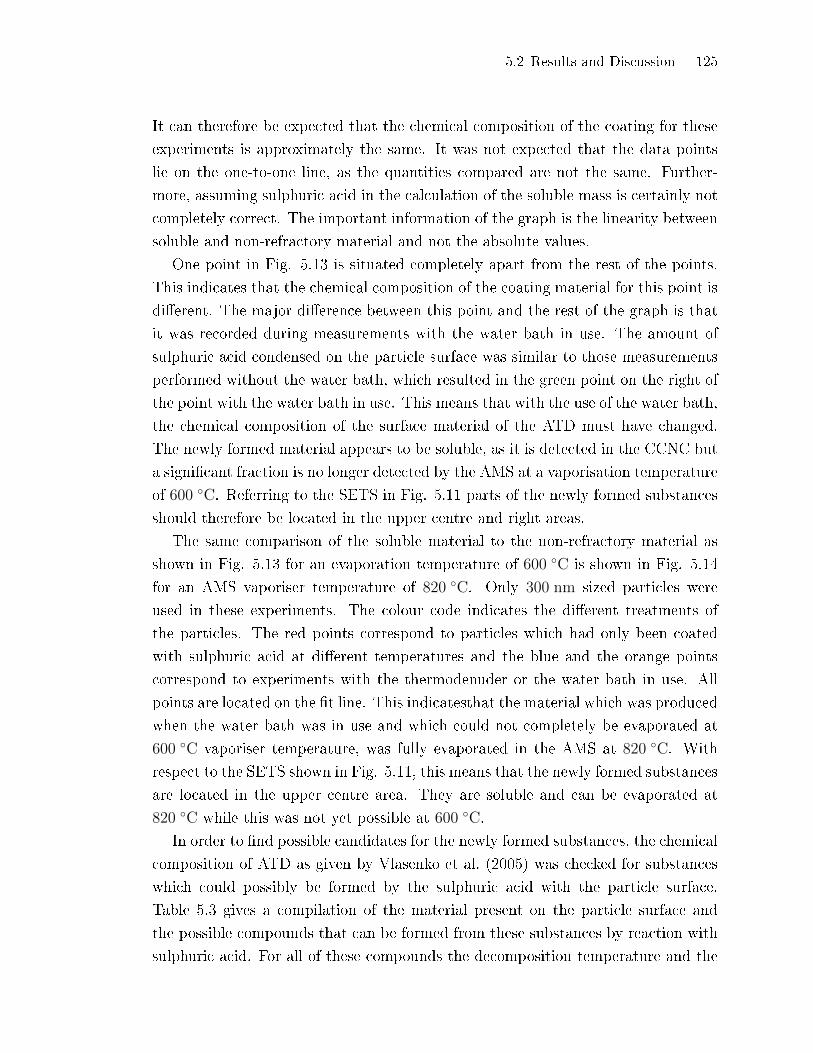
5.2 Results and Discussion 125
It can therefore be expected that the chemical composition of the coating for these
experiments is approximately the same. It was not expected that the data points
lie on the one-to-one line, as the quantities compared are not the same. Further-
more, assuming sulphuric acid in the calculation of the soluble mass is certainly not
completely correct. The important information of the graph is the linearity between
soluble and non-refractory material and not the absolute values.
One point in Fig. 5.13 is situated completely apart from the rest of the points.
This indicates that the chemical composition of the coating material for this point is
di�erent. The major di�erence between this point and the rest of the graph is that
it was recorded during measurements with the water bath in use. The amount of
sulphuric acid condensed on the particle surface was similar to those measurements
performed without the water bath, which resulted in the green point on the right of
the point with the water bath in use. This means that with the use of the water bath,
the chemical composition of the surface material of the ATD must have changed.
The newly formed material appears to be soluble, as it is detected in the CCNC but
a signi�cant fraction is no longer detected by the AMS at a vaporisation temperature
of 600 ◦C. Referring to the SETS in Fig. 5.11 parts of the newly formed substances
should therefore be located in the upper centre and right areas.
The same comparison of the soluble material to the non-refractory material as
shown in Fig. 5.13 for an evaporation temperature of 600 ◦C is shown in Fig. 5.14
for an AMS vaporiser temperature of 820 ◦C. Only 300 nm sized particles were
used in these experiments. The colour code indicates the di�erent treatments of
the particles. The red points correspond to particles which had only been coated
with sulphuric acid at di�erent temperatures and the blue and the orange points
correspond to experiments with the thermodenuder or the water bath in use. All
points are located on the �t line. This indicatesthat the material which was produced
when the water bath was in use and which could not completely be evaporated at
600 ◦C vaporiser temperature, was fully evaporated in the AMS at 820 ◦C. With
respect to the SETS shown in Fig. 5.11, this means that the newly formed substances
are located in the upper centre area. They are soluble and can be evaporated at
820 ◦C while this was not yet possible at 600 ◦C.
In order to �nd possible candidates for the newly formed substances, the chemical
composition of ATD as given by Vlasenko et al. (2005) was checked for substances
which could possibly be formed by the sulphuric acid with the particle surface.
Table 5.3 gives a compilation of the material present on the particle surface and
the possible compounds that can be formed from these substances by reaction with
sulphuric acid. For all of these compounds the decomposition temperature and the
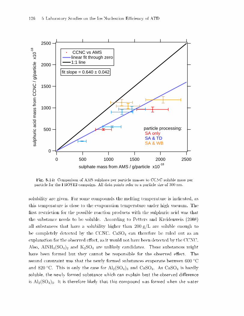
126 5 Laboratory Studies on the Ice Nucleation E�ciency of ATD
2500
2000
1500
1000
500
0
sulp
huric
aci
d m
ass
from
CC
NC
/ g/
part
icle
x10
-18
25002000150010005000
sulphate mass from AMS / g/particle x10-18
fit slope = 0.640 ± 0.042
CCNC vs AMSlinear fit through zero1:1 line
particle processing: SA only SA & TD SA & WB
Fig. 5.14: Comparison of AMS sulphate per particle masses to CCNC soluble mass perparticle for the FROST2 campaign. All data points refer to a particle size of 300 nm.
solubility are given. For some compounds the melting temperature is indicated, as
this temperature is close to the evaporation temperature under high vacuum. The
�rst restriction for the possible reaction products with the sulphuric acid was that
the substance needs to be soluble. According to Petters and Kreidenweis (2008)
all substances that have a solubility higher than 200 g/L are soluble enough to
be completely detected by the CCNC. CaSO4 can therefore be ruled out as an
explanation for the observed e�ect, as it would not have been detected by the CCNC.
Also, AlNH4(SO4)2 and K2SO4 are unlikely candidates. These substances might
have been formed but they cannot be responsible for the observed e�ect. The
second constraint was that the newly formed substances evaporate between 600 ◦C
and 820 ◦C. This is only the case for Al2(SO4)3 and CaSO4. As CaSO4 is hardly
soluble, the newly formed substance which can explain best the observed di�erence
is Al2(SO4)3. It is therefore likely that this compound was formed when the water
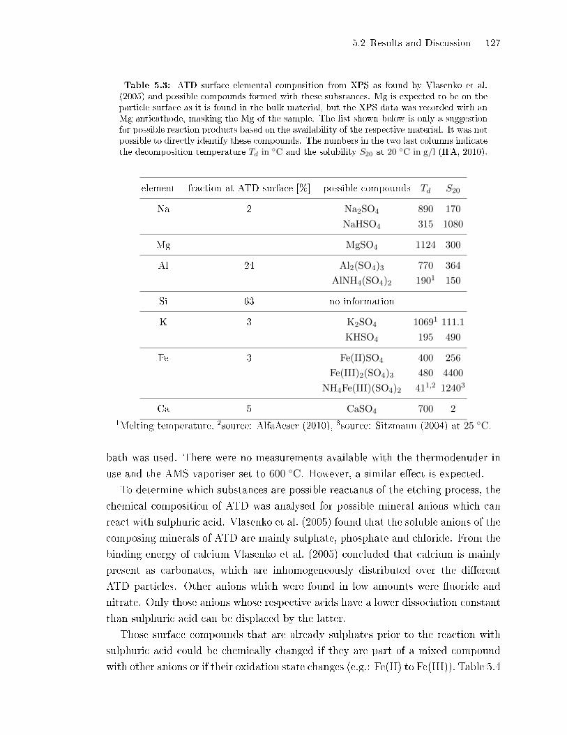
5.2 Results and Discussion 127
Table 5.3: ATD surface elemental composition from XPS as found by Vlasenko et al.(2005) and possible compounds formed with these substances. Mg is expected to be on theparticle surface as it is found in the bulk material, but the XPS data was recorded with anMg anticathode, masking the Mg of the sample. The list shown below is only a suggestionfor possible reaction products based on the availability of the respective material. It was notpossible to directly identify these compounds. The numbers in the two last columns indicatethe decomposition temperature Td in ◦C and the solubility S20 at 20
◦C in g/l (IFA, 2010).
element fraction at ATD surface [%] possible compounds Td S20
Na 2 Na2SO4 890 170
NaHSO4 315 1080
Mg - MgSO4 1124 300
Al 24 Al2(SO4)3 770 364
AlNH4(SO4)2 1901 150
Si 63 no information - -
K 3 K2SO4 10691 111.1
KHSO4 195 490
Fe 3 Fe(II)SO4 400 256
Fe(III)2(SO4)3 480 4400
NH4Fe(III)(SO4)2 411,2 12403
Ca 5 CaSO4 700 2
1Melting temperature, 2source: AlfaAeser (2010), 3source: Sitzmann (2004) at 25 ◦C.
bath was used. There were no measurements available with the thermodenuder in
use and the AMS vaporiser set to 600 ◦C. However, a similar e�ect is expected.
To determine which substances are possible reactants of the etching process, the
chemical composition of ATD was analysed for possible mineral anions which can
react with sulphuric acid. Vlasenko et al. (2005) found that the soluble anions of the
composing minerals of ATD are mainly sulphate, phosphate and chloride. From the
binding energy of calcium Vlasenko et al. (2005) concluded that calcium is mainly
present as carbonates, which are inhomogeneously distributed over the di�erent
ATD particles. Other anions which were found in low amounts were �uoride and
nitrate. Only those anions whose respective acids have a lower dissociation constant
than sulphuric acid can be displaced by the latter.
Those surface compounds that are already sulphates prior to the reaction with
sulphuric acid could be chemically changed if they are part of a mixed compound
with other anions or if their oxidation state changes (e.g.: Fe(II) to Fe(III)). Table 5.4

128 5 Laboratory Studies on the Ice Nucleation E�ciency of ATD
Table 5.4: Compilation of the dissociation constants of the acids corresponding to the an-ions found in ATD. Those anions which are located below the sulphate ion, can be displacedby sulphuric acid. Source: Jander et al. (2002)
pka by dissociation level
anion abundance in ATD [a.u.] 1 2 3
Cl− 0.7 -7
SO2−4 41 -3 1.92
NO−3 0.2 -1.32
PO3−4 3 2.13 7.20 12.36
F− 0.1 3.14
CO2−3 NA1 6.52 10.40
SiO4−4 9.512 11.742 NA
1Not quanti�ed by Vlasenko et al. (2005) but their XPS data showed that Ca was
associated with carbonates on the particle surface.2Source: Widberg and Fischer (2007)
shows the anions found by Vlasenko et al. (2005) with their respective concentration.
The mass fractions these concentrations correspond to are not given. Except for
chloride, all anions shown in this table can be displaced from their salts by sulphuric
acid as their acid dissociation constants pka are higher than the pka of sulphuric
acid in the �rst dissociation step. In its second dissociation level, sulphuric acid
can no longer displace nitrate from its salts but is still strong enough to displace
phosphates, �uorides, and carbonates. It can therefore be concluded that most of
the anions present in the particle which are not part of the silicate structure can be
etched by sulphuric acid. The silicate structure itself may also be etched considering
the pka of silicic acid, of which SiO2 is the anhydride form. However, the solubility
of silicic acid is very low. The condensation of water on the aerosol surface could
nevertheless solve a minor fraction of potentially formed silicic acid and thus the
alumino-silicates are a potential source for aluminium that can form Al2(SO4)3.
Kaolinite is a mineral which is known to act as IN ((e.g.: Lüönd et al., 2010, Mur-
ray et al., 2011, Salam et al., 2006, Welti et al., 2009)). Colina et al. (2002) reported
that the alumino silicate kaolin, which is mainly constituted of kaolinite reacts with
sulphuric acid when heated. If at least parts of the alumino-silicates of the ATD are
present in the crystalline form of kaolinite, it is possible that these are responsible for
the ATD ice nucleus e�ciency. The heating with the thermodenuder could increase
the reaction of the sulphuric acid with this mineral and therefore reduce the ATD
ability to act as an IN. The study by Colina et al. (2002) showed that Al2(SO4)3 is
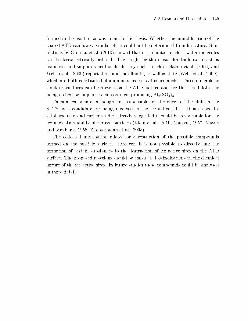
5.2 Results and Discussion 129
formed in the reaction as was found in this thesis. Whether the humidi�cation of the
coated ATD can have a similar e�ect could not be determined from literature. Sim-
ulations by Croteau et al. (2010) showed that in kaolinite trenches, water molecules
can be ferroelectrically ordered. This might be the reason for kaolinite to act as
ice nuclei and sulphuric acid could destroy such trenches. Salam et al. (2006) and
Welti et al. (2009) report that montmorillonite, as well as illite (Welti et al., 2009),
which are both constituted of alumino-silicates, act as ice nuclei. These minerals or
similar structures can be present on the ATD surface and are thus candidates for
being etched by sulphuric acid coatings, producing Al2(SO4)3.
Calcium carbonate, although not responsible for the e�ect of the shift in the
SETS, is a candidate for being involved in the ice active sites. It is etched by
sulphuric acid and earlier studies already suggested it could be responsible for the
ice nucleation ability of aerosol particles (Klein et al., 2010, Manson, 1957, Mason
and Maybank, 1958, Zimmermann et al., 2008).
The collected information allows for a restriction of the possible compounds
formed on the particle surface. However, it is not possible to directly link the
formation of certain substances to the destruction of ice active sites on the ATD
surface. The proposed reactions should be considered as indications on the chemical
nature of the ice active sites. In future studies these compounds could be analysed
in more detail.


6
Aerosol Cloud Interaction Experiments at the AIDA
This chapter describes experiments performed at the AIDA facility at the KIT in
Karslruhe. Since the evaluation of the data showed weaknesses in the experimental
method with respect to the use of an AMS, the goal of this chapter is to show how
the experiments can be improved in order to adjust the experimental conditions to
the measurement capacities of the AMS.
6.1 E�ect of Cloud Processing on Aerosol Composition
During the laboratory measurement campaign ACI-03 (Aerosol Cloud Interaction)
experiments were performed with ambient air in the AIDA chamber (see Sect. 2.2.4).
Filling the AIDA with ambient aerosol produces a realistic starting composition
of the aerosol. In the experiment described in the following, the ambient aerosol
particles in the chamber were sampled with an AMS before and after an expansion
of the air in the chamber.
During the expansion, the pressure in the chamber was reduced from 1008 mbar to
approximately 780 mbar. The starting temperature was 264 K. Thus, when re�lling
the chamber to ambient pressure with �ltered air, the aerosol was diluted by a factor
of 0.77. Additionally the particle number concentration is reduced by a factor of
2 in the AIDA chamber in the time between two expansions. However, the mass
concentration measured with the AMS was constant during the time the AMS was
measuring between the expansions, as shown in Fig. 6.1. During the expansion, the
humidity in the chamber reached saturation with respect to water after ∼ 40 s and
a supersaturation of 10 % was reached ∼ 25 s later. At a supersaturation of 10 % all
particles larger than ∼ 30 nm are activated with respect to the Kelvin e�ect alone
(Eq. (1.1)). Therefore all particles which are transmitted into the AMS should have
become activated as CCN at this supersaturation. The maximum supersaturation
reached is 40 %. As the supersaturation lasted for more than a quarter of an hour,
some of the droplets probably sedimented and removed the aerosol within. Figure 6.2
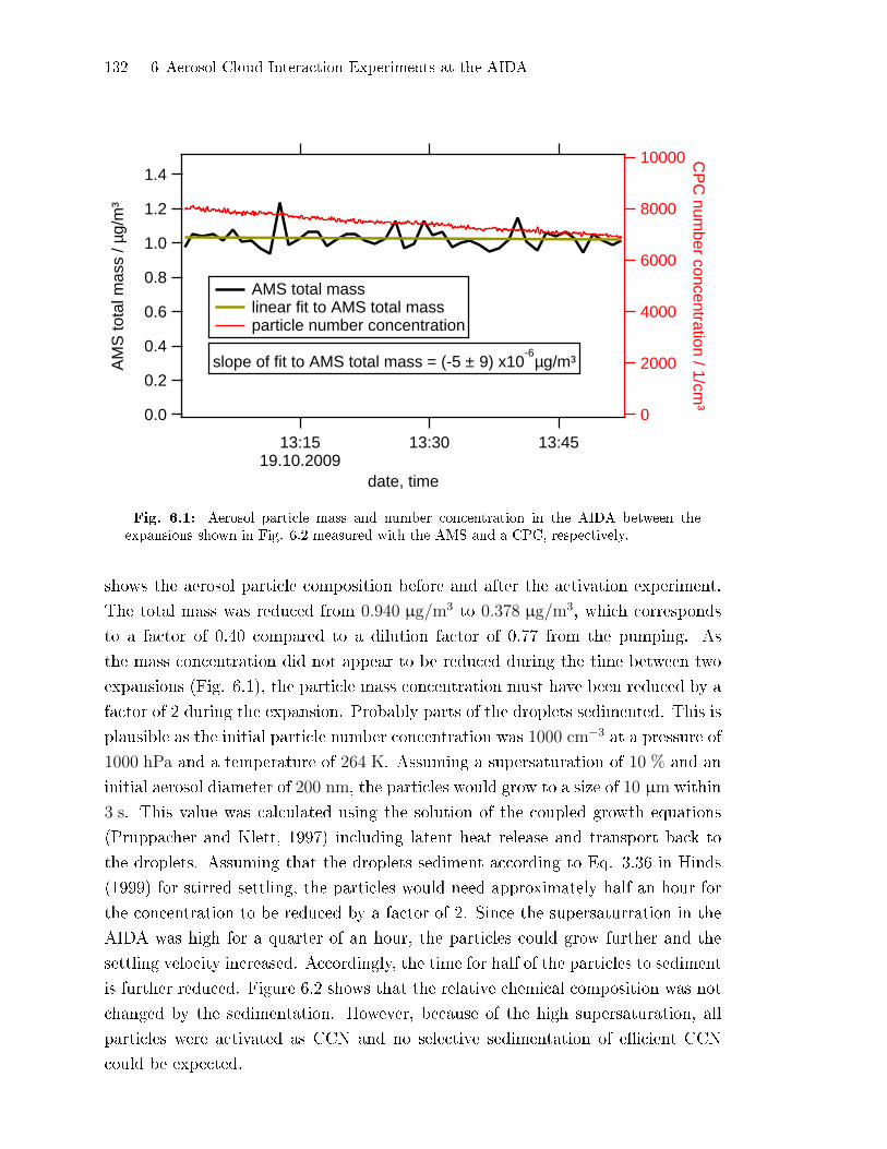
132 6 Aerosol Cloud Interaction Experiments at the AIDA
1.4
1.2
1.0
0.8
0.6
0.4
0.2
0.0
AM
S to
tal m
ass
/ µg/
m³
13:1519.10.2009
13:30 13:45
date, time
10000
8000
6000
4000
2000
0
CP
C num
ber concentration / 1/cm³
slope of fit to AMS total mass = (-5 ± 9) x10-6
µg/m³
AMS total mass linear fit to AMS total mass particle number concentration
Fig. 6.1: Aerosol particle mass and number concentration in the AIDA between theexpansions shown in Fig. 6.2 measured with the AMS and a CPC, respectively.
shows the aerosol particle composition before and after the activation experiment.
The total mass was reduced from 0.940 µg/m3 to 0.378 µg/m3, which corresponds
to a factor of 0.40 compared to a dilution factor of 0.77 from the pumping. As
the mass concentration did not appear to be reduced during the time between two
expansions (Fig. 6.1), the particle mass concentration must have been reduced by a
factor of 2 during the expansion. Probably parts of the droplets sedimented. This is
plausible as the initial particle number concentration was 1000 cm−3 at a pressure of
1000 hPa and a temperature of 264 K. Assuming a supersaturation of 10 % and an
initial aerosol diameter of 200 nm, the particles would grow to a size of 10 µm within
3 s. This value was calculated using the solution of the coupled growth equations
(Pruppacher and Klett, 1997) including latent heat release and transport back to
the droplets. Assuming that the droplets sediment according to Eq. 3.36 in Hinds
(1999) for stirred settling, the particles would need approximately half an hour for
the concentration to be reduced by a factor of 2. Since the supersaturration in the
AIDA was high for a quarter of an hour, the particles could grow further and the
settling velocity increased. Accordingly, the time for half of the particles to sediment
is further reduced. Figure 6.2 shows that the relative chemical composition was not
changed by the sedimentation. However, because of the high supersaturation, all
particles were activated as CCN and no selective sedimentation of e�cient CCN
could be expected.
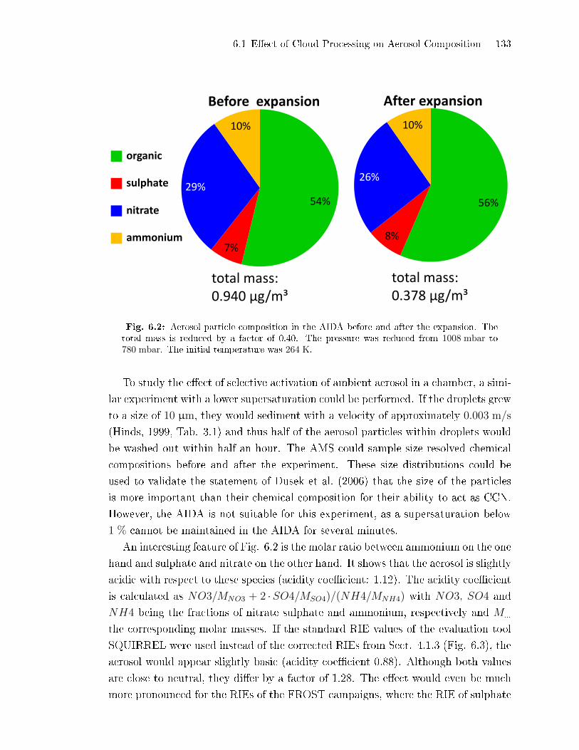
6.1 E�ect of Cloud Processing on Aerosol Composition 133
54%
7%
29%
10%
Before expansion
Org
SO4
NO3
NH4
56%
8%
26%
10%
After expansion
total mass: 0.940 µg/m³
total mass: 0.378 µg/m³
organic
sulphate
nitrate
ammonium
Fig. 6.2: Aerosol particle composition in the AIDA before and after the expansion. Thetotal mass is reduced by a factor of 0.40. The pressure was reduced from 1008 mbar to780 mbar. The initial temperature was 264 K.
To study the e�ect of selective activation of ambient aerosol in a chamber, a simi-
lar experiment with a lower supersaturation could be performed. If the droplets grew
to a size of 10 µm, they would sediment with a velocity of approximately 0.003 m/s
(Hinds, 1999, Tab. 3.1) and thus half of the aerosol particles within droplets would
be washed out within half an hour. The AMS could sample size resolved chemical
compositions before and after the experiment. These size distributions could be
used to validate the statement of Dusek et al. (2006) that the size of the particles
is more important than their chemical composition for their ability to act as CCN.
However, the AIDA is not suitable for this experiment, as a supersaturation below
1 % cannot be maintained in the AIDA for several minutes.
An interesting feature of Fig. 6.2 is the molar ratio between ammonium on the one
hand and sulphate and nitrate on the other hand. It shows that the aerosol is slightly
acidic with respect to these species (acidity coe�cient: 1.12). The acidity coe�cient
is calculated as NO3/MNO3 + 2 ·SO4/MSO4)/(NH4/MNH4) with NO3, SO4 and
NH4 being the fractions of nitrate sulphate and ammonium, respectively and M...
the corresponding molar masses. If the standard RIE values of the evaluation tool
SQUIRREL were used instead of the corrected RIEs from Sect. 4.1.3 (Fig. 6.3), the
aerosol would appear slightly basic (acidity coe�cient 0.88). Although both values
are close to neutral, they di�er by a factor of 1.28. The e�ect would even be much
more pronounced for the RIEs of the FROST campaigns, where the RIE of sulphate

134 6 Aerosol Cloud Interaction Experiments at the AIDA
49%
11%
27%
13%
Before expansion
Org
SO4
NO3
NH4
total mass: 1.028 µg/m³
total mass: 0.427 µg/m³
organic
sulphate
nitrate
ammonium
51%
12%
24%
13%
After expansion
Fig. 6.3: Data shown in Fig. 6.2 without the application of the correction factors for theRIE.
was reduced and the RIE of ammonium was increased. This should be kept in mind
when calculating acidity ratios for ambient aerosol and the RIE should be published
along with the results.
6.2 Detection of Coating on Mineral Dust During Cloud
Activation Experiments
One of the objectives of the AMS measurements during the ACI-03 campaign was to
quantify the amount of coating on mineral dust particles. This was possible under
some assumptions for the FROST campaigns (Chapt. 5) during which monodisperse
aerosol was used. During ACI-03, the probed mineral dust was polydisperse. This
caused major fractions of the dust to be outside the transmission range of the AMS
aerodynamic inlet lens for all experiments. In contrast to the FROST campaigns,
it was not possible to correct for these transmission losses as no size distributions
for monodisperse particles relevant for the aerosol inside the AIDA chamber were
available for the AMS. Due to losses and coagulation inside the chamber, the aerosol
size distribution was changing gradually and thus it would have been necessary to
monitor it continuously. Scanning mobility particle sizer (SMPS) measurements are
not optimal for such a monitoring, as they monitor the number size distribution of
the aerosol and not the surface size distribution. The count rate for bigger particles,

6.2 Detection of Coating on Mineral Dust During Cloud Activation Experiments 135
12x109
10
8
6
4
2
0
dS/d
log(
d mob
) [n
m²
/ cm
³]
9100
2 3 4 5 6 7
dmob [nm]
700
600
500
400
300
200
100
0
dN/dlog(d
mob ) [1/cm
³]
Surface distribution lognormal fit:mode diameter = 383 nmGSD = 1.55
SMPS surface area size distribution lognormal fit SMPS number size distribution
Fig. 6.4: Number size distribution measured with an SMPS and surface size distributioncalculated from the number size distribution. Note the low signal to noise ratio at highdiameters due to low counting rates. The total particle concentration in the AIDA was∼ 350 1/cm3. The size distribution of this �gure was averaged for close to two hours.
which are relevant for the surface size distribution was low and thus the uncertainty
was high.
Figure 6.4 shows the number size ditribution measured with an SMPS of the Asian
Dust samples (AD2) used during ACI-03 together with the surface size distribution.
The surface size distribution is an approximation of the mass size distribution as
measured by the AMS for the case of thin coatings. As no size distribution of
the dust from the AMS was available, several parameters had to be approximated.
In the size range of the maximum surface, the SMPS measurement only provided
low counting rates, resulting in a very noisy signal and thus a very uncertain �t
maximum, ranging between 350 and 450 nm (Fig 6.4). This uncertainty had to
be considered when calculating the transmission of the instrument. Additionally,
as no AMS size distributions for the aerosol in the chamber were available, it was
impossible to exactly determine the Jayne shape factor (see Eq. (4.1)). This intro-
duces an additional error in the determination of the mode diameter of the aerosol
in the AIDA. As the Jayne shape factor is not identical for all particles but shows a
distribution, the size distribution of the aerosol is broadened by an unknown factor.
To estimate the range of the correction factors, a density of 2.6 g/cm3, a Jayne
shape factor between 0.77 and 1, as well as a Jayne shape factor distribution width
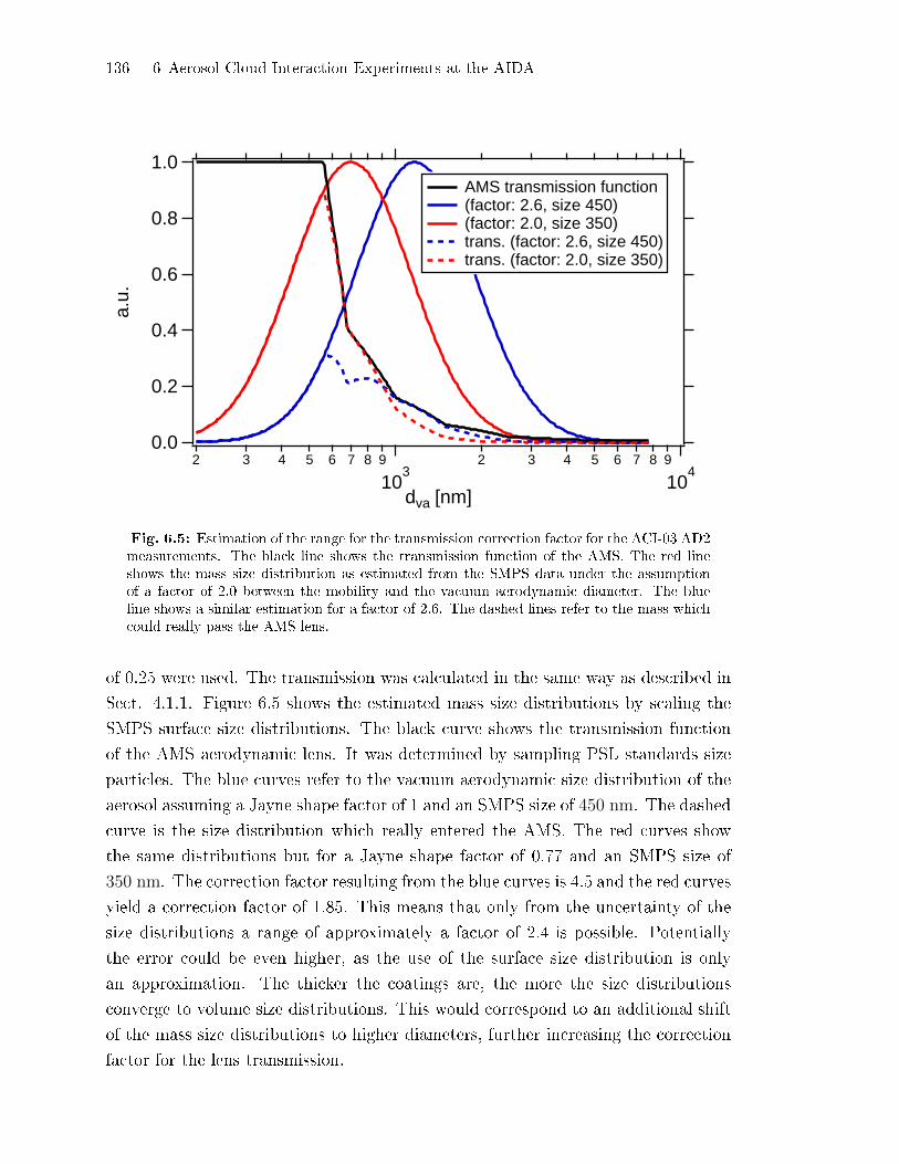
136 6 Aerosol Cloud Interaction Experiments at the AIDA
1.0
0.8
0.6
0.4
0.2
0.0
a.u.
2 3 4 5 6 7 8 9
103
2 3 4 5 6 7 8 9
104
dva [nm]
AMS transmission function (factor: 2.6, size 450) (factor: 2.0, size 350) trans. (factor: 2.6, size 450) trans. (factor: 2.0, size 350)
Fig. 6.5: Estimation of the range for the transmission correction factor for the ACI-03 AD2measurements. The black line shows the transmission function of the AMS. The red lineshows the mass size distribution as estimated from the SMPS data under the assumptionof a factor of 2.0 between the mobility and the vacuum aerodynamic diameter. The blueline shows a similar estimation for a factor of 2.6. The dashed lines refer to the mass whichcould really pass the AMS lens.
of 0.25 were used. The transmission was calculated in the same way as described in
Sect. 4.1.1. Figure 6.5 shows the estimated mass size distributions by scaling the
SMPS surface size distributions. The black curve shows the transmission function
of the AMS aerodynamic lens. It was determined by sampling PSL standards size
particles. The blue curves refer to the vacuum aerodynamic size distribution of the
aerosol assuming a Jayne shape factor of 1 and an SMPS size of 450 nm. The dashed
curve is the size distribution which really entered the AMS. The red curves show
the same distributions but for a Jayne shape factor of 0.77 and an SMPS size of
350 nm. The correction factor resulting from the blue curves is 4.5 and the red curves
yield a correction factor of 1.85. This means that only from the uncertainty of the
size distributions a range of approximately a factor of 2.4 is possible. Potentially
the error could be even higher, as the use of the surface size distribution is only
an approximation. The thicker the coatings are, the more the size distributions
converge to volume size distributions. This would correspond to an additional shift
of the mass size distributions to higher diameters, further increasing the correction
factor for the lens transmission.
6.2 Detection of Coating on Mineral Dust During Cloud Activation Experiments 137
The goal of the AMS measurements was to quantify the surface coating thickness
of the dust in the AIDA chamber. To do so, it would have been necessary to nor-
malise the mass concentrations to the particle's total surface area. This again would
have involved the calculation of surface size distributions from particle counts, which
again would have introduced a big uncertainty. Additionally, the uncertainties of
the correction factors described in Sect. 4.1 add to the above presented uncertain-
ties. Finally, the calibration error of the AMS is assumed to be 30 %. With all
these uncertainties, it is impossible to give any reliable quanti�cation of the aersol
coatings in the AIDA chamber.
In future studies these obstacles could be overcome by the use of a new aerody-
namic lens which operates at higher pressures and can therefore focus particles in a
higher size range. This type of lens is still being characterised but it can potentially
focus particles of up to 3 µm. In addition, experiments with size selected particles
should be performed with every type of dust used in the chamber in order to better
access the Jayne shape factor of the aerosol as well as its distribution. With these
modi�cations the experiments would be more suitable for the application of an AMS
and the quanti�cation of coatings on mineral dust particles would be possible for
the experimental situation at the AIDA.

7
Conclusions and Outlook
In this study the AMS was used during three laboratory measurement campaigns,
FROST1 and FROST2 at the LACIS facility at the IfT in Leipzig and the ACI-03
campaign at the AIDA facility at the KIT in Karlsruhe. In all three campaigns, the
e�ect of coatings on mineral dust ice nuclei was investigated. For the FROST1 and
FROST2 the characterisation of thin sulphuric acid coatings on ATD particles was
successfully performed.
As the instrument was operated with very low signals, the mathematical tools to
analyse the detection limits of the AMS were improved. Di�erent methods have been
tested to obtain satisfactory results. It is now possible to calculate detection limits
of the AMS under operation conditions, without losing precious time by sampling
through a particle �lter, and without being restricted to periods with a constant
closed signal.
The characterisation of the instrument was improved to enable correct quanti�-
cation of the sulphate loadings on the ATD particle surfaces. Correction factors for
the instrument inlet transmission, the collection e�ciency, and the relative ionisa-
tion e�ciency have been determined. Using these corrections, the mass per particle
loadings of the ATD after the condensation of sulphuric acid on its surface could be
calculated.
Combining AMS results to ice nucleus counter results revealed that the IN-
e�ciency of ATD is reduced by the condensation of sulphuric acid on the particle's
surfaces. The reason for this reduction was not the covering of the particle's surface
but a chemical reaction of sulphuric acid with the particle's surface. This reactions
were accelerated when the aerosol was humidi�ed or heated after the coating with
sulphuric acid. Evidence for the stronger reaction of the sulphuric acid with the
ATD surface when heated or humidi�ed was given by the reduction of the hydro-
gen containing fragments, which were identi�ed as proxies for sulphuric acid and
140 7 Conclusions and Outlook
ammonium sulphate, and which are missing if the sulphate originates from metal
sulphates.
A further indication for the production of new chemical compounds was the
change of the position of the sulphate containing compounds in the solubility-
evaporation temperature space. This information was retrieved by comparing the
soluble mass per particle deduced from CCNC measurement with the non-refractory
mass per particle deduced from the AMS data recorded at 600 ◦C and 820 ◦C. The
newly formed substance which is responsible for the shift in the SETS is most likely
Al2(SO4)3. However, it was not possible to determine whether the formation of this
substance is responsible for the loss of the IN-ability of ATD. A further compound
of interest is CaCO3 as it is contained in the ATD and is also likely to react with
sulphuric acid.
Future Work
A direct identi�cation of the reactions that took place on the ATD surface was not
possible but further explorations of the SETS could restrict the possible compounds.
The soluble mass could be measured with a particle into liquid sampler (PILS) or a
similar instrument which can directly access the soluble mass fraction of the aerosol.
An instrument that could potentially directly detect the surface compounds is the
single particle laser ablation instrument SPLAT2 (Zelenyuk et al., 2009). Due to the
two step ablation and ionisation it can be used to selectively evaporate the surface
of particles.
The main result of this study, namely that sulphuric acid reduces ATD ice nu-
cleation ability through surface etching, can be used in theoretical studies on the
nature of ice nuclei. The structure studied need to be sensitive to sulphuric acid
etching and the addition of water must increase the reaction kinetics.
Croteau et al. (2010) showed in simulations that water can start freezing in
trenches in kaolinite. Based on these simulations it is feasible to analyse kaolinite
particles for trenches on their surface using transmission electron microscopy. These
particles could be used afterwards for immersion freezing experiments on a cold
stage as described by Murray et al. (2011). The idea is to determine whether those
particles with the more pronounced trenches are also the best ice nuclei. The same
e�ect could be expected for other clay mineral particles which are known to be good
ice nuclei, like e.g. montmorillonite and illite. Both of these minerals are alumino
silicates and could, regarding to the chemical composition of ATD, be present on
the ATD surface.
7 Conclusions and Outlook 141
The same evaluation applied on the ATD can also be applied to other mineral
dust systems. The interesting question is whether the reduction of the IN-ability
can always be connected to particle surface reactions.
To improve the atmospheric relevance of this type of experiments, the aerosol
preparation at the LACIS facility will be modi�ed in a way to produce the sulphuric
acid from gas phase SO2 which is oxidised and humidi�ed to form sulphuric acid in
the carrier air of the particles. This avoids exposing the particles to atmospherically
unrealistic high temperature over the sulphuric acid bath. Similar studies are also
planned with nitric acid.
The data collected with the AMS at the AIDA facility could not be evaluated
reliably due to very high uncertainties in the necessary instrument inlet transmis-
sion correction factors. This can be avoided in future studies by the use of a new
aerodynamic inlet lens which is optimised for the transmission of larger particles.
In order to verify the predominance of the size e�ect over the chemistry e�ect
in the CCN activation behaviour, the following cloud activation experiment is pro-
posed: An AIDA-like expansion chamber could be �lled with ambient air to get an
atmospherically relevant aerosol. An expansion experiment is performed with a low
expansion rate to get only low, atmospherically relevant supersaturations to selec-
tively activate the most e�cient CCN. The AMS could measure before and after the
expansion, increasing its sampling time compared to measurements of the activated
fraction during an expansion experiment and allowing to get chemically resolved size
distributions before and after the expansion. These chemically resolved size distri-
butions could be compared to see which size fraction and which chemical fraction
of the aerosol sedimented and must therefore have been activated. The challenge
of this experiment is to achieve low supersaturations in an expansion chamber for
several minutes. The advantage of such a measurement is that the competition of
the droplets for water vapour is simulated on a realistic time scale. Furthermore
the AMS can measure for a long period before and after the experiment. This way
it can sample long enough to retrieve size distributions which are clearly above the
detection limit.

List of Figures
1.1 Köhler equation with Kelvin and Raoult term. . . . . . . . . . . . . . . . . . . . . 4
2.1 Schematics of the AMS modi�ed after Drewnick et al. (2005).
ptof: particle time of �ight, MCP: multi channel plate, preamp:
preampli�er, ADC: analog digital converter. . . . . . . . . . . . . . . . . . . . . . 10
2.2 Exemplary size calibration recorded during the measurement
campaign ACI-03 by measuring PSL size standards. The error bars
are calculated from the estimated uncertainties of the particle time
of �ight (34 µs), the uncertainty of the �ight distance in the AMS
vacuum chamber (5 mm) and a 2 % error in the calibration particle
mobility diameter. . . . . . . . . . . . . . . . . . . . . . . . . . . . . . . . . . . . . . . . . . . . . 12
2.3 Screen shot of the AMS baseline determination window. The y-axis
is inverted. The green line is the signal as recorded with the MCP
at low voltage. The blue line is the baseline and the red line is the
baseline plus the threshold. . . . . . . . . . . . . . . . . . . . . . . . . . . . . . . . . . . . . 13
2.4 E�ect of thresholding on a signal. The upper graph shows the signal
with the threshold level marked in green and the lower graph depicts
the signal after the threshold was applied. . . . . . . . . . . . . . . . . . . . . . . . . 14
2.5 Screen shot of the AMS SI calibration window. The peak shown is
the averaged signal of 2380 single ion events. . . . . . . . . . . . . . . . . . . . . . 15
2.6 AMS ion optics introducing the ions created in the ioniser into the
mass spectrometer. . . . . . . . . . . . . . . . . . . . . . . . . . . . . . . . . . . . . . . . . . . . 16
2.7 TEM picture of two ATD particles. Note the di�erence in the aspect
ratio between the two particles indicated by the red circle and the
blue oval. (TEM picture by A. Kiselev, Institute for Tropospheric
Research, Leipzig and I. Lieberwirth, MPI-P, Mainz) . . . . . . . . . . . . . 21

144 LIST OF FIGURES
2.8 Sulphuric acid coating unit used during the FROST campaigns. The
aerosol enters the coating unit in a glass tube and passes over a
small heated sulphuric acid bath. To control the temperature, the
sulphuric acid bath section is surrounded by a water bath. The
temperature of the water is maintained by a heating unit below the
table.) . . . . . . . . . . . . . . . . . . . . . . . . . . . . . . . . . . . . . . . . . . . . . . . . . . . . . 23
3.1 a) Organic closed signal recorded during one �ight of the
measurement campaign POLARCAT. The noise standard deviations
for of the FFT b) Squared amplitudes of the Fast Fourier
Transformation of the signal shown in a). c) Illustation of the
periodic continuation of the signal for the FFT with discontinuities
at the matching points. . . . . . . . . . . . . . . . . . . . . . . . . . . . . . . . . . . . . . . . . 28
3.2 Closed signal (red) with a Bezier curve (green, explained in Sect.
3.2.2) using the signal points as vertices for the calculation of the
curve. The Bezier curve was subtracted from the closed signal
resulting in a detrended curve (blue) which can be used to calculate
the standard deviation of the noise of the closed time series. The
region named ��at region� can be used to directly estimate the closed
signal noise level by calculating the standard deviation of the closed
signal. The noise level calculated by the Bezier curve detrending and
the DL-cubic algorithm are shown on the graph. They agree perfectly. 30
3.3 Illustration of the problem to �nd a running mean which detrends a
curve well in all situations. Upper graph: Using a binomial running
mean window with a width of 50 points detrends the curve well.
Lower graph: The same running mean window used in this curve
results in an overestimation of the noise level. . . . . . . . . . . . . . . . . . . . . 31
3.4 Schematics of the construction of one point of a Bezier curve. The
blue points represent the signal which is smoothed. . . . . . . . . . . . . . . . . 33
3.5 a) Generated signal. b) Generated Gaussian noise. c) Generated
signal with generated nosie added. d) Curve from �c)� with Bezier
curve. e) Estimated noise after the detrending using the Bezier curve. 36
3.6 Generated signals with normal noise with a standard deviation of
0.01. Each �gure shows the signal together with an attempted
detrending with a Bezier curve calculated directly using the signal
points as vertices. The signal equations are listed in Tab. 3.1. The
relative errors were calculated using Eq. (3.6) . . . . . . . . . . . . . . . . . . . . 37
LIST OF FIGURES 145
3.7 Summary of the results from the tests of the noise level determination
using Bezier curves to detrend the signal. For each function from
Tab. 3.1 the average relative deviation of the estimated noise from
the input noise (Eq. (3.6)) is presented. The red bars were obtained
when the whole detrended signal was used to estimate the standard
deviation. The blue bars refer to the situation that the 5 points
closest to the signal edge were omitted in the calculation of the
estimated noise. This way, disturbances from the signal edges were
avoided. . . . . . . . . . . . . . . . . . . . . . . . . . . . . . . . . . . . . . . . . . . . . . . . . . . . . . 38
3.8 a) Generated signal with Bezier detrending. The standard deviation
is underestimated by 28 % b) Generated signal with linearly
extrapolated edges which reduce the underestimation of the noise
standard deviation to 24 %. . . . . . . . . . . . . . . . . . . . . . . . . . . . . . . . . . . . . 40
3.9 Example of a situation in which the Bezier method worked �ne. a):
Signal (red) with a Bezier curve. Middle graph: Good detrended
signal. . . . . . . . . . . . . . . . . . . . . . . . . . . . . . . . . . . . . . . . . . . . . . . . . . . . . . . 42
3.10 Example of a situation in which the Bezier method worked bad.
Upper graph: Signal (red) with a Bezier curve. Middle graph: Badly
detrended signal. Lower Graph: Alternative detreding using the
DL-cubic . . . . . . . . . . . . . . . . . . . . . . . . . . . . . . . . . . . . . . . . . . . . . . . . . . . . 43
3.11 Local �t of a signal by a third order polynomial with the centre
point omitted. The green points hi and Hi mark the interpolated
central points. For the ideal signal f (left graph) it is approximately
equal to the central point of the curve. In the case of a real signal
with noise F , Fi and Hi di�er by Ei. . . . . . . . . . . . . . . . . . . . . . . . . . . . . 44
3.12 Distribution of the result of DL-cubic for 100,000 signals with a
length of 1000 points. The standard noise level of these signals was 5.0. 50
3.13 Relative deviation ∆σbase,rel of the DL-cubic output distribution
(Eq. (3.24)) vs. 1√N−4 . . . . . . . . . . . . . . . . . . . . . . . . . . . . . . . . . . . . . . . . . 51
3.14 a) Evolution of the algorithm output with increasing number of
signal points per in�ection point for a sine function without noise.
b) Sine function with 6.25 signal points per in�ection point as an
example for the lower limit of the sample rate for the algorithm to
work properly. . . . . . . . . . . . . . . . . . . . . . . . . . . . . . . . . . . . . . . . . . . . . . . . 54
3.15 Plots of the test functions divers1 to divers6. The output of the
DL-cubic for these functions is shown in Tab. 3.4. . . . . . . . . . . . . . . . . . 55
3.16 Plots of the test functions step1 to step5 . . . . . . . . . . . . . . . . . . . . . . . . . 57
146 LIST OF FIGURES
3.17 Function divers2 with noise and a histogram of the results of the
algorithm used with this function. The standard deviation of the
noise was 0.05. . . . . . . . . . . . . . . . . . . . . . . . . . . . . . . . . . . . . . . . . . . . . . . . 58
3.18 Decay of the detection limits of di�erent species after a pump
exchange. The detection limits were determined for 30 s averaging
time. . . . . . . . . . . . . . . . . . . . . . . . . . . . . . . . . . . . . . . . . . . . . . . . . . . . . . . . . 62
3.19 Roughly detrended beam open and beam closed signals of the
period after the pump exchange shown in Fig. 3.18. The correlation
coe�cient R2 is clearly increased in the red period, indicating that
the variations of the signal are not of random nature. . . . . . . . . . . . . . . 63
3.20 Distribution of the ratio of the output of the DL-cubic to the classic
method. . . . . . . . . . . . . . . . . . . . . . . . . . . . . . . . . . . . . . . . . . . . . . . . . . . . . . 64
3.21 Comparison of the results of the continuous method to the counting
statistics. The noise level was estimated for every m/z using the
new method and by calculating counting statistics. The data was
�tted using Eq. (3.36). . . . . . . . . . . . . . . . . . . . . . . . . . . . . . . . . . . . . . . . 66
3.22 Comparison of the model using constant random noise to the output
of the DL-cubic-algorithm . . . . . . . . . . . . . . . . . . . . . . . . . . . . . . . . . . . . . 68
3.23 Comparison of the electronic noise (upper panel) to the recorded
electronic noise after thresholding (lower panel). The panel in the
middle shows a signal with noise added and the threshold is marked
in green. . . . . . . . . . . . . . . . . . . . . . . . . . . . . . . . . . . . . . . . . . . . . . . . . . . . . 69
3.24 Illustration of the signal dependent noise. The left axis is equal to
the number k of SISs and the x-axis are the time bins. The dots
represent SISs which are recorded in the time bins and the numbers
on the dots are referred to in the text. . . . . . . . . . . . . . . . . . . . . . . . . . . . 70
3.25 Comparison of the model using signal dependent random noise to
the output of the DL-cubic . . . . . . . . . . . . . . . . . . . . . . . . . . . . . . . . . . . . 72
3.26 Ratio of the �tted noise levels to the experimentally determined
noise levels as calculated with the new algorithm. The green line
refers to a �tting with signal dependent noise being taken into
account while the red line results from a �t with only assuming a
constant random noise level. . . . . . . . . . . . . . . . . . . . . . . . . . . . . . . . . . . . 75
LIST OF FIGURES 147
3.27 Comparison of the ratios between the �ts to the noise using Eq.
(3.51) for two di�erent experiments but with similar instrument
setting. The graph shows that the discrepancies are of systematic
nature and are thus unlikely to be DL-cubic-artefacts which would
be expected to behave randomly. . . . . . . . . . . . . . . . . . . . . . . . . . . . . . . . 76
4.1 Silicone size distributions for 200 nm mobility diameter particles
with log normal �t. Upper graph: BCR, averaged over 1 h 20 min.
Lower graph: ATD, averaged over 5 h 39 min. dmod is the modal
diamter of the log normal �t and GSD is the geometric standard
deviation of the size distribution. The errors correspond to the
�tting uncertainties. . . . . . . . . . . . . . . . . . . . . . . . . . . . . . . . . . . . . . . . . . . 80
4.2 Transmission correction for BCR and ATD particles. The �gures
show the projected transmission curves as calculated from the �ts
in Fig. 4.1 as well as the projected size distribution when the
transmission of the aerodynamic lens is taken into account. . . . . . . . . . 81
4.3 Collection e�ciency (CE) for all experiments using coated BCR
particles. The categories refer to di�erent experimental conditions.
The �rst number is the dmob, the second the temperature of
the sulphuric acid bath used for the coating. WB indicates
humidi�cation of the particles with a water bath and TD indicates
the use of a thermodenuder at the temperature following TD. Every
data point was averaged over ∼ 106 particles. The error bars were
calculated from Gaussian error propagation using the standard
deviations of the mean values for the time series of the mass per
particle corresponding to the data points and the con�dence intervals
of the soluble mass per particle determined with the CCNC. . . . . . . . 84
4.4 Comparison of the results of the measurements pepeated during the
CE determination measurements to the FROST1 campaign. . . . . . . . 86
4.5 E�ect of the correction for high background slope on the CCM
signal. Carbon containing material (CCM) is a combination of
organics and carbonates. . . . . . . . . . . . . . . . . . . . . . . . . . . . . . . . . . . . . . . . 89
4.6 Summary of the correction factors which need to be applied to the
di�erent AMS mass loadings to get correct quantitative results. . . . . . 90
5.1 Experimental set-up of the FROST campaigns. The sections between
the �uidized bed generator and the DMA can be bypassed. . . . . . . . . . 94

148 LIST OF FIGURES
5.2 Coating of ATD with sulphuric acid. On the transmission electron
microscope picture the thickness of an 6 nm coating is indicated to
give an idea of how thin the coatings in this study were. 6 nm is a
rather thick coating. . . . . . . . . . . . . . . . . . . . . . . . . . . . . . . . . . . . . . . . . . 96
5.3a Average AMS mass spectrum for unprocessed ATD during the
FROST1 campaign. Notable are the peaks at m/z 73 and 147 that
can be attributed to methyl silicone contaminant. . . . . . . . . . . . . . . . . . 98
5.3b Average AMS mass spectrum for untreated ATD during the FROST2
campaign. Beside the silicone peaks already visible during FROST1,
some new very distinct metal peaks show up in this spectrum, due
to the elevated vaporiser temperature of 820 ◦C: 23Na+, 39K+, 41K+,85Rb+, 87Rb+, 133Cs+ and 135Ba+. . . . . . . . . . . . . . . . . . . . . . . . . . . . . . . 99
5.3c Average AMS mass spectrum of sulphuric acid processed ATD
during the FROST2 campaign. The sulphuric acid bath temperature
was 70 ◦C. Beside the sulphate peaks in red, the metal peaks that
were already visible in the unprocessed 820 ◦C data remain visible.
The silicone probably reacted with the sulphuric acid to SiO2 that is
not detected. . . . . . . . . . . . . . . . . . . . . . . . . . . . . . . . . . . . . . . . . . . . . . . . . . 100
5.4 Sulphate mass concentration measured with the AMS together with
the particle number concentration from CPC measurements for one
day of the FROST1 campaign. The vertical lines indicate the limits
of the measurement intervals. Lines with the same colour delimit
one interval. . . . . . . . . . . . . . . . . . . . . . . . . . . . . . . . . . . . . . . . . . . . . . . . . . 102
5.5 Sulphate mass per particle concentration for the same day as shown
in Fig. 5.4. The mass per particle was calculated by normalising the
mass concentrations measured with the AMS to the particle number
concentrations from CPC measurements. The vertical lines indicate
the limits of the measurement intervals. Lines with the same colour
delimit one interval. . . . . . . . . . . . . . . . . . . . . . . . . . . . . . . . . . . . . . . . . . . . 103
5.6a Summary of the mass per particle for the FROST1 campaign
(Experiments 1-11, recorded at 600 ◦C AMS vaporiser temperature).
The left axis refers to sulphate and CCM, the right axis refers to
silicone. Note the factor of 10 between the axes. On the horizontal
axis, the second line shows the particle size, the third one indicates
if the water bath was used, the fourth one if ammonium was added.
The last line refers to the temperature of the sulphuric acid coating
section. . . . . . . . . . . . . . . . . . . . . . . . . . . . . . . . . . . . . . . . . . . . . . . . . . . . . . 105

LIST OF FIGURES 149
5.6b Summary of the mass per particle for the FROST2 campaign
thinnest coating experiments (Experiments 12-18, recorded at 820 ◦C
AMS vaporiser temperature). All particles had a mobility diameter
of 300 nm. The left axis refers to sulphate and CCM, the right
axis refers to silicone. Note the factor of 10 between the axes. On
the horizontal axis, the second line now shows the thermodenuder
temperature in contrast to Fig. 5.3a, the third one indicates if the
water bath was used, the fourth one if ammonium was added. The
last line refers to the temperature of the sulphuric acid coating section.109
5.6c Summary of the mass per particle for the FROST2 campaign thicker
coating experiments (Experiments 19-32, recorded at 820 ◦C AMS
vaporiser temperature). All particles had a mobility diameter
of 300 nm. The left axis refers to sulphate and CCM, the right
axis refers to silicone. Note the factor of 10 between the axes.
On the horizontal axis, the second line shows the thermodenuder
temperature, the third one indicates if the water bath was used, the
fourth one if ammonium was added. The lr marked in the special line
refers to an experiment with an additional residence volume of 10 L
after the particle coating. The last line refers to the temperature of
the sulphuric acid coating section. . . . . . . . . . . . . . . . . . . . . . . . . . . . . . . 111
5.7 Comparison of AMS sulphate per particle masses to the CFDC ice
nuclei counts at −30 ◦C in the immersion-freezing regime. Di�erent
coating temperatures are shown for the di�erent particle classes. The
particle class �pure� includes those experiments with no treatment
and no sulphuric acid condensation. The particle class �SA only�
includes particles which passed the sulphuric acid bath but no
further processing was performed and �WB� indicates the additional
use of the water bath. The IN-activity of the ATD is reduced if more
sulphuric acid is condensed on the particle surface and the use of the
water bath decreases the number of IN even further. The error bars
of the mass concentrations were determined as described in Sect.
5.2.2. . . . . . . . . . . . . . . . . . . . . . . . . . . . . . . . . . . . . . . . . . . . . . . . . . . . . . . 114

150 LIST OF FIGURES
5.8 Comparison of AMS sulphate per particle masses to the LACIS
ice nucleus counts at −35 ◦C during FROST2. Di�erent sulphuric
acid bath temperatures are shown for every particle class. The
particle class �pure� includes those experiments with no treatment
and no sulphuric acid condensation. The particle class �SA only�
includes particles which passed the sulphuric acid bath but no
further processing was performed. �WB� indicates the additional use
of the water bath and �TD� the additional use of the thermodenuder
after the treatment except for the blue point on the upper left which
refers to particles which passed the thermodenuder but were not
coated. The error bars of the mass concentrations were determined
as described in Sect. 5.2.2. . . . . . . . . . . . . . . . . . . . . . . . . . . . . . . . . . . . . . 115
5.9 Comparison of the possible fragments attributed to sulphate
depending on the sulphate compound. For ammonium sulphate
and sulphuric acid, hydrogen containing fragments are produced in
the vaporisation and ionisation process while metal sulphate salts
cannot produce such fragments. Typical examples for metals could
be aluminium, iron or calcium. . . . . . . . . . . . . . . . . . . . . . . . . . . . . . . . . . 119
5.10 Intensity of the fragments HSO+3 (m/z = 81) and H2SO
+4 (m/z =
98) normalised to the intensity of the fragment SO+2 (m/z = 64)
for the FROST2 campaign. The �rst line on the horizontal axis
shows the thermodenuder temperature, the second one indicates if
the water bath was used and the third one if ammonium was added.
The lr marked in the special line refers to an experiment with an
additional residence volume of 10 L after the particle coating. The
last line refers to the temperature of the sulphuric acid coating section.120
5.11 Scheme of the solubility-evaporation temperature space. The left
axis indicates increasing solubility and the bottom axis refers to
increasing evaporation temperature. The space is roughly divided
into six areas. The text in each area indicates whether the AMS and
the CCNC are able to detect material situated in the respective region.122
5.12 Fictive example of a CCNC activation curve. At ∼ 0.103 %
supersaturation, half of the particles activated as cloud droplets.
This supersaturation is considered to be the critical supersaturation
and thus corresponds to the maximum of the Köhler curve (Eq. (2.2)).123
LIST OF FIGURES 151
5.13 Comparison of AMS sulphate per particle masses to CCNC soluble
mass per particle for the FROST1 campaign. The point strongly
deviating from the linear �t was recorded with the water bath in
use. All other points refer to experiments during which the particles
were coated with sulphuric acid without further processing. . . . . . . . . 124
5.14 Comparison of AMS sulphate per particle masses to CCNC soluble
mass per particle for the FROST2 campaign. All data points refer
to a particle size of 300 nm. . . . . . . . . . . . . . . . . . . . . . . . . . . . . . . . . . . . . 126
6.1 Aerosol particle mass and number concentration in the AIDA
between the expansions shown in Fig. 6.2 measured with the AMS
and a CPC, respectively. . . . . . . . . . . . . . . . . . . . . . . . . . . . . . . . . . . . . . . 132
6.2 Aerosol particle composition in the AIDA before and after the
expansion. The total mass is reduced by a factor of 0.40. The
pressure was reduced from 1008 mbar to 780 mbar. The initial
temperature was 264 K. . . . . . . . . . . . . . . . . . . . . . . . . . . . . . . . . . . . . . . . 133
6.3 Data shown in Fig. 6.2 without the application of the correction
factors for the RIE. . . . . . . . . . . . . . . . . . . . . . . . . . . . . . . . . . . . . . . . . . . 134
6.4 Number size distribution measured with an SMPS and surface size
distribution calculated from the number size distribution. Note the
low signal to noise ratio at high diameters due to low counting rates.
The total particle concentration in the AIDA was ∼ 350 1/cm3. The
size distribution of this �gure was averaged for close to two hours. . . . 135
6.5 Estimation of the range for the transmission correction factor for the
ACI-03 AD2 measurements. The black line shows the transmission
function of the AMS. The red line shows the mass size distribution
as estimated from the SMPS data under the assumption of a factor
of 2.0 between the mobility and the vacuum aerodynamic diameter.
The blue line shows a similar estimation for a factor of 2.6. The
dashed lines refer to the mass which could really pass the AMS lens. . 136


List of Tables
3.1 Test functions used for the evaluation of the performance of the
Bezier detrending method. The �rst �ve curves are signals which
produce visually good detrending (EXP, 2EXP, EXPX2, GAUSS,
QUAD) while the following three functions are visually badly
detrended. The last function is a simple constant signal with noise,
representing the extreme case of no variation of the signal. l is the
length of the signal. . . . . . . . . . . . . . . . . . . . . . . . . . . . . . . . . . . . . . . . . . . . 35
3.2 Relative errors (Eq. (3.6)) of a subset of the Bezier �tting tests in
%. �der. . . � refers to the derivatives used for the determination
of the locations of the vertices. �long� means that the signal was
extrapolated by 20 points to either side and short means that no
extrapolation was done. . . . . . . . . . . . . . . . . . . . . . . . . . . . . . . . . . . . . . . . 41
3.3 Overview of the symbols used to calculate the uncertainty intervals
of the DL-cubic-algorithm . . . . . . . . . . . . . . . . . . . . . . . . . . . . . . . . . . . . . 52
3.4 �Zero�-values of the algorithm for the six test functions divers1 to
divers6 where no noise was added. . . . . . . . . . . . . . . . . . . . . . . . . . . . . . . 56
3.5 �Zero�-values of the algorithm for the �ve step functions . . . . . . . . . . . 56
3.6 Results of the application of the DL-cubic algorithm on the function
used to test the Bezier detrending method showed in Tab. 3.2. . . . . . . 58
3.7 Comparison of the algorithm outputs for the step functions described
in Tab. 3.5 without outlier detection (un�ltered) to the results when
the �ltering for outliers was applied (�ltered). For these tests normal
noise with an amplitude of 0.01 was added to the signal. The table
shows the average output for 1000 di�erent noise functions together
with the estimated standard deviations. . . . . . . . . . . . . . . . . . . . . . . . . . 60
154 LIST OF TABLES
3.8 Comparison of the detection limits calculated with DL-cubic to the
detection limits found by Drewnick et al. (2009) and DeCarlo et al.
(2006). The values shown always refer to an averaging time of 30 s.
The DeCarlo et al. (2006) values have been multiplied by√2 to be
comparable. . . . . . . . . . . . . . . . . . . . . . . . . . . . . . . . . . . . . . . . . . . . . . . . . . . 64
3.9 Comparison of the DL calculated by the classic method compared to
the DL-cubic based method. The averaging interval was 10 s. . . . . . . . 65
3.10 Overview of the parameters in the �tting equation (3.51) . . . . . . . . . . 73
3.11 Fitting values corresponding to the curve in Fig. 3.25 with σ = 1.2 . 74
4.1 Transmission correction factors: The errors have been estimated by
varying the mode diameter and the geometric width in the range of
the �tting parameter uncertainties of the lognormal distribution. . . . . 82
4.2 Relative ionisation e�ciencies (RIE) for the species sulphate and
ammonium for the FROST1 and FROST2 campaign and the ACI-03
campaign . . . . . . . . . . . . . . . . . . . . . . . . . . . . . . . . . . . . . . . . . . . . . . . . . . . . 88
5.1 Mobility, volume equivalent and aerodynamic diameters of the
particles used in this study, including the sizes which correspond to
doubly charged particles passing the DMA. . . . . . . . . . . . . . . . . . . . . . . 95
5.2 Sulphuric acid coating thickness of the FROST1 campaign. Note
that the AMS could not detect all of the sulphate material with the
vaporiser set to 600 ◦C. A fraction of the sulphuric acid reacted with
the particle surface and formed refractory metal sulphates. . . . . . . . . . 107
5.3 ATD surface elemental composition from XPS as found by Vlasenko
et al. (2005) and possible compounds formed with these substances.
Mg is expected to be on the particle surface as it is found in the bulk
material, but the XPS data was recorded with an Mg anticathode,
masking the Mg of the sample. The list shown below is only a
suggestion for possible reaction products based on the availability
of the respective material. It was not possible to directly identify
these compounds. The numbers in the two last columns indicate the
decomposition temperature Td in ◦C and the solubility S20 at 20◦C
in g/l (IFA, 2010). . . . . . . . . . . . . . . . . . . . . . . . . . . . . . . . . . . . . . . . . . . . . 127
5.4 Compilation of the dissociation constants of the acids corresponding
to the anions found in ATD. Those anions which are located below
the sulphate ion, can be displaced by sulphuric acid. Source: Jander
et al. (2002) . . . . . . . . . . . . . . . . . . . . . . . . . . . . . . . . . . . . . . . . . . . . . . . . . 128
List of Symbols and Abbreviations
Abbrevations
Explantion
ACI-03 Aerosol Cloud Interaction-03
AD2 Asian Dust sample 2
AIDA Aerosol Interaction and Dynamics in the Atmosphere
AMS Aerosol Mass Spectrometer
ATD Arizona Test Dust
BCR BCR-66 quartz size standards; Acronym signi�cance is
not known.
BFSP Brute Force Single Particle
C-TOF-AMS Compact Time Of Flight Aerosol Mass Spectrometer
CAD Computer-Aided Design
CCM Carbon Containing Material
CCN Cloud Condensation Nucleus
CCNC Cloud Condensation Nucleus Counter
CE Collection E�ciency
CFDC Continuous Flow Di�usion Chamber
CPC Condensation Particle Counter
DL Detection Limit
DMA Di�erential Mobility Analyser
FFT Fast Fourier Transformation
FROST FReezing Of duST
GSD Geometric Standard Deviation
HR-TOF-AMS High Resolution Time Of Flight Aerosol Mass Spec-
trometer
IN Ice Nucleus

156 List of Symbols and Abbreviations
KIT Karlsruhe Institute of Technology
LACIS Leipzig Aerosol Cloud Interaction Simulator
MCP Multi Channel Plate
MS Mass Spectrum
PILS Particle Into Liquid Sampler
POLARCAT POLar study using Aircraft, Remote sensing, surface
measurements and modelling of Climate, chemistry,
Aerosols and Transport
PSL PolyStyrol Latex
PTOF Particle Time Of Flight
Q-AMS Quadrupole Aerosol Mass Spectrometer
RIE Relative Ionisation E�ciency
SETS Solubility-Evaporation-Temperature Space
SIS Single Ion Signal
SQUIRREL SeQUential Igor data RetRiEvaL
TEM Transmission Electron Microscope
XPS X-ray Photoelectron Spectroscopy
Symbols
Explantion unit
α Parameter of the Cunningham slip correction factor cal-
culation
α Random noise
A Factor of the Kelvin term m
A Particle surface area nm2
Ai Fitting parameter of the Hi at location i
ai Fitting parameter of the hi at location i
Aduty Factor of the duty cycle correction u0.5 eV−0.5
Bi Fitting parameter of the of Hi at location i
bi Fitting parameter of the of hi at location i
Ci Fitting parameter of the Hi at location i
ci Fitting parameter of the hi at location i
Di Fitting parameter of the Hi at location i
di Fitting parameter of the hi at location i
β Parameter of the Cunningham slip correction factor cal-
culation
List of Symbols and Abbreviations 157
B Factor of the Raoult term m3
Bi,n Bernstein polynomials
CE Collection e�ciency
Cc Cunningham slip correction factor
Cj Complex intensities of the Fourier spectrum frequencies
CS Mass Concentration µgm−3
CDL-cubic Computational complexity of the DL-cubic-algorithm
CBezier Computational complexity of the Bezier detrending
method
D Diameter of the wet particle nm
da Aerodynamic diameter nm
Dp Particle diameter nm
DATD Projected mass size distribution
dcoat Coating thickness nm
Dcrit Critical diameter for cloud activation nm
Ddry Diameter of the dry particle nm
dic E�ective diameter of the insoluble core in the modi�ed
Köhler equation
nm
dmob Mobility diameter nm
dmod Modal diameter nm
dve Volume equivalent diameter nm
dva Vacuum aerodynamic diameter nm
ε Gaussian noise
εi Volume fraction of soluble material
E Detrended signal using the DL-cubic-algorithm
∆F Activation energy for crossing the liquid water/ice
boundary
J
fAB Average airbeam correction factor
F Signal with noise
f Ideal signal without noise
fAB Airbeam correction factor
Fpuls Number of pulses of the mass spectrometer per second s−1
ftrans Transmission function of the AMS aerodynamic lens
∆Ghet Gibbs free energy for the formation of a critical ice em-
bryo
J
γ Amplitude of the electronic noise

158 List of Symbols and Abbreviations
γ Parameter of the Cunningham slip correction factor cal-
culation
H Third order local polynomial �tting functions to F
h Planck constant J s
h Third order local polynomial �tting functions to f
∆I Modelled counts noise level of the AMS ion
∆Idiff Counting statistics error ion
IE Ionisation e�ciency ionmolec−1
I Counts signal of the AMS ion
i Index
IS Ion count rate s−1
Iclosed Ion counts in closed mode ion
Iopen Ion counts in open mode ion
j Factor indicating how many standard deviations the
DL-cubic-output is over or underestimating the real
value
j Index
jhet Heterogenous freezing rate molec s−1m−3
εcoat Volume fraction of the particle coating material
εcore Volume fraction of the particle core material
κi Apparent hygroscopicity parameters
κapp Apparent hygroscopicity parameter
κcoat Apparent hygroscopicity of the particle coating
κcore Apparent hygroscopicity of the particle core
k Boltzmann constant JK−1
k Iteration step of the de Casteljau-algorithm
k Number of SIS
k Number of active sites per surface and di�erential tem-
perature interval
m−2K−1
kcomp Correction factors needed to compare the FROST cam-
paigns, determined by a recalibration of the AMS-CPC-
dilution-stage-system to the CCNC
ktrans Correction factor for the AMS lens transmission
λ Mean free path of air nm
l Length of a generated signal
∆mppcor Uncertainty of the AMS mass per particle including all
correction factors
ag
List of Symbols and Abbreviations 159
MW NO3 Molecular weight of nitrate gmol−1
µ Mean value of a distribution
m/z Mass to charge ratio u eV−1
MSiO2 Molecular weight of silicon oxide gmol−1
Mw Molecular weight of water gmol−1
mppcor AMS mass per particle including all correction factors ag
mppraw AMS mass per particle prior to the application of the
correction factors
ag
msoluble Soluble mass per particle loading ag
N Number of points of an AMS signal
N Number of time bins
N ′ Number of points of a Fourier transformed AMS signal
NA Avogadro number molecmol−1
na Surface density of ice active sites m−2
ns Number density of water molecules at the ice nu-
cleus/water interface
molecm−2
ns Number of solute moles mol
NATD Number of molecules contained in the ATD core mate-
rial
molec
Ncoat Number of coating molecules molec
Ncrit Critical value for the the number of points of a signal
for which the DL-cubic-algorithm can be applied with
a desired precision of j standard deviations.
ωj Frequencies of the Fourier transformed spectrum s−1
O Order function of the computational complexity~Pi De�ning polygon of a Bezier curve (in this thesis: the
AMS closed signal)
p(k,N) Probability that in a time series with N time bins, the
kth SIS is recorded in a time bin which did not include
an SIS before
p◦ Water saturation vapour pressure over a �at water sur-
face
Pa
pw Saturation vapour pressure over a droplet Pa
Qin Average AMS inlet �ow rate
Qin Inlet �ow rate cm3 s−1
RIE Relative ionisation e�ciency
ρ0 Unit density: 1 g/cm3 g cm−3
160 List of Symbols and Abbreviations
ρH2SO4 Density of sulphuric acid: 1.8356× 10⁻³ ag/nm3 ag nm−3
ρp Particle density g cm−3
ρw Density of water kgm−3
ρcoat Density of the coating g cm−3
~r Bernstein-Bezier-curve
R Standard deviation of the DL-cubic detrended signal E
R Universal gas constant Jmol−1K−1
∆σ... Abbrevation for ∆σbase and ∆σalgo
∆σalgo Estimate of ∆σbase from σalgo using Eq. (3.25)
∆σbase,rel Ratio of the standard deviation of the algorithm out-
puts ∆σbase to the real standard deviation of the input
noise σbase
∆σbase Standard deviation of the algorithm outputs
∆σrel Relative di�erence between σinput and σest
σ Factor of the broadening of the counting statistics error
due to variations of the intensity between di�erent SISs
σ Standard deviation of the noise of an AMS closed signal µgm−3
σw Surface tension of water Nm−1
σ... Abbrevation for σbase and ∆σalgo
σalgo Output of the DL-cubic-algorithm for one signal
σbase Standard deviation of the basic population of the ran-
dom numbers used to test the DL-cubic-algorithm
σcnt Counts noise level
σest Standard deviation of the estimated pure noise using a
Bezier curve
σfilter Standard deviation of a �lter measurement
σinput Standard deviation of the noise added to a generated
signal
σmc Mass concentration noise level µgm−3
S Jayne shape factor
S Scaling factor which accounts for the di�erence between
Tint and the real width of a time bin
S20 Solubility at 20 ◦C g l−1
Scrit Critical saturation ratio for cloud activation
S Saturation ratio
dθ Di�erential temperature interval K
T Temperature K

List of Symbols and Abbreviations 161
T Time spend averaging one m/z during a DL determi-
nation period
s
ti Location i on the time axis
Tclosed Time spent in AMS closed mode s
Tint Time integrating the signal which is attributed to one
m/z during one pulse of the mass spectrometer
ns
tmeas Total time spent measuring with the AMS during one
DL determination period
s
Topen Time spent in AMS open mode s
Uion Voltage of the ion chamber V
Vcoat Volume of the particle coating nm3
VSI Unit conversion factor equal to the area below a single
ion signal
bit ns
Vtotal Total volume of the particle nm3
χ Dynamic shape factor
xpulser Open length of the pulser electrode of the mass spec-
trometer
mm
z Parameter referring to the position on a Bezier curve.
z ∈ [0, 1]


Publications Originating from this Thesis
Niedermeier, D., Hartmann, S., Shaw, R. A., Covert, D., Mentel, T. F., Schneider,
J., Poulain, L., Reitz, P., Spindler, C., Clauss, T., Kiselev, A., Hallbauer, E., Wex,
H., Mildenberger, K., and Stratmann, F.: Heterogeneous freezing of droplets with
immersed mineral dust particles - measurements and parameterization, Atmo-
spheric Chemistry and Physics, 10, 3601�3614, 2010.
Niedermeier, D., Hartmann, S., Clauss, T., Wex, H., Kiselev, A., Sullivan, R. C.,
DeMott, P. J., Petters, M. D., Reitz, P., Schneider, J., Mikhailov, E., Sierau,
B., Stetzer, O., Reimann, B., Bundke, U., Shaw, R. A., Buchholz, A., Mentel,
T. F., and Stratmann, F.: Experimental study of the role of physicochemical
surface processing on the IN ability of mineral dust particles, Atmos. Chem. Phys.
Discuss., 11, 18 557�18 588, doi:10.5194/acpd-11-18557-2011, 2011.
Reitz, P., Schneider, J., Wex, H., Stratmann, F., Niedermeier, D., Mildenberger, K.,
Covert, D., Mentel, T. F., Spindler, C., Poulain, L., and Borrmann, S.: Detection
of thin coatings on refractory particles with an Aerosol Mass Spectrometer: Ap-
plication in laboratory studies of hygroscopic growth, CCN and IN activation, in:
European Aerosol Conference, poster presentation, 2009a.
Reitz, P., Schneider, J., Wex, H., Stratmann, F., Niedermeier, D., Mildenberger,
K., Covert, D., Mentel, T. F., Spindler, C., Poulain, L., and Borrmann, S.: Thin
Coatings On Refractory Particles: Detection With Mass Spectrometry And Im-
plications For Studies Of Hygroscopic Growth, CCN And IN Activation, in: In-
ternational Conference on Nucleation and Atmospheric Aerosol, talk, 2009b.
Reitz, P., Schneider, J., Wex, H., Stratmann, F., Niedermeier, D., Mildenberger,
K., Hartmann, S., Kiselev, A., Shaw, R., Covert, D., Buchholz, A., Spindler, C.,
Mentel, T. F., Poulain, L., Sullivan, R. C., DeMott, P. J., Petters, M. D., and
Borrmann, S.: Surface modi�cation of mineral dust particles by thin coatings: Im-

164 PUBLICATIONS ORIGINATING FROM THIS THESIS
plications for CCN and IN abilities, in: International Aerosol Conference, poster
presentation which received a Best Poster Prize, 2010.
Reitz, P., Spindler, C., Mentel, T. F., Poulain, L., Wex, H., Mildenberger, K., Nie-
dermeier, D., Hartmann, S., Clauss, T., Stratmann, F., Sullivan, R. C., DeMott,
P. J., Petters, M. D., Sierau, B., and Schneider, J.: Surface modi�cation of mineral
dust particles by sulphuric acid processing: implications for CCN and IN abilities,
Atmos. Chem. Phys. Discuss., 11, 7235�7289, doi:10.5194/acpd-11-7235-2011,
2011.
Sullivan, R. C., Petters, M. D., DeMott, P. J., Kreidenweis, S. M., Wex, H., Nieder-
meier, D., Hartmann, S., Clauss, T., Stratmann, F., Reitz, P., Schneider, J., and
Sierau, B.: Irreversible loss of ice nucleation active sites in mineral dust particles
caused by sulphuric acid condensation, Atmospheric Chemistry and Physics, 10,
11 471�11 487, doi:10.5194/acp-10-11471-2010, 2010.
References
Abbatt, J. P. D., Benz, S., Cziczo, D. J., Kanji, Z., Lohmann, U., and Möhler,
O.: Solid ammonium sulfate aerosols as ice nuclei: A pathway for cirrus cloud
formation, Science, 313, 1770�1773, doi:10.1126/science.1129726, 2006.
Albrecht, B. A.: Aerosols, cloud microphysics, and fractional cloudiness, Science,
245, 1227�1230, 1989.
AlfaAeser: data sheet ammonium iron(III) sulphate, 2010.
Alfarra, M. R., Coe, H., Allan, J. D., Bower, K. N., Boudries, H., Canagaratna,
M. R., Jimenez, J. L., Jayne, J. T., Garforth, A. A., Li, S. M., and Worsnop,
D. R.: Characterization of urban and rural organic particulate in the lower Fraser
valley using two aerodyne aerosol mass spectrometers, Atmospheric Environment,
38, 5745�5758, doi:10.1016/j.atmosenv.2004.01.054, 2004.
Allan, J. D.: Error Calculation for AMS Analysis (talk AMS user meet-
ing 2010), URL http://cires.colorado.edu/jimenez-group/UsrMtgs/UsersMtg11/
JDAerrorpresentation.pdf, 2010.
Allan, J. D., Jimenez, J. L., Williams, P. I., Alfarra, M. R., Bower, K. N.,
Jayne, J. T., Coe, H., and Worsnop, D. R.: Quantitative sampling using an
Aerodyne aerosol mass spectrometer. 1. Techniques of data interpretation and
error analysis, Journal of Geophysical Research, 108, AAC1�1�AAC1�10, doi:
10.1029/2002jd002358, 2003.
Allan, J. D., Delia, A. E., Coe, H., Bower, K. N., Alfarra, M. R., Jimenez, J. L.,
Middlebrook, A. M., Drewnick, F., Onasch, T. B., Canagaratna, M. R., Jayne,
J. T., and Worsnop, D. R.: A generalised method for the extraction of chemically
resolved mass spectra from aerodyne aerosol mass spectrometer data, Journal of
Aerosol Science, 35, 909�922, doi:10.1016/j.jaerosci.2004.02.007, 2004.
166 REFERENCES
Bahreini, R., Jimenez, J. L., Jian, W., Flagan, R. C., Seinfeld, J. H., Jayne, J. T.,
and Worsnop, D. R.: Aircraft-based aerosol size and composition measurements
during ACE-Asia using an Aerodyne aerosol mass spectrometer, Journal of Geo-
physical Research, 108, ACE13�1�ACE13�ACE13�22, doi:10.1029/2002jd003226,
2003.
Barnett, V. and Lewis, T.: Outliers in statistical data, Wiley Series in Probabil-
ity & Statistics, John Wiley and Sons, Chichester New York Brisbane Toronto
Singapore, 3rd edn., 1994.
Bronstein, I., Semendjajew, K., Musiol, G., and Mühlig, H.: Taschenbuch der
Mathematik, Wissenschaftlicher Verlag Harri Deutsch GmbH, Frankfurt amMain,
2008.
Canagaratna, M. R., Jayne, J. T., Jimenez, J. L., Allan, J. D., Alfarra, M. R., Zhang,
Q., Onasch, T. B., Drewnick, F., Coe, H., Middlebrook, A., Delia, A., Williams,
L. R., Trimborn, A. M., Northway, M. J., DeCarlo, P. F., Kolb, C. E., Davidovits,
P., and Worsnop, D. R.: Chemical and microphysical characterization of ambi-
ent aerosols with the aerodyne aerosol mass spectrometer, Mass Spectrometry
Reviews, 26, 185�222, doi:10.1002/mas.20115, 2007.
Carslaw, K. S., Wirth, M., Tsias, A., Luo, B. P., Dornbrack, A., Leutbecher, M.,
Volkert, H., Renger, W., Bacmeister, J. T., and Peter, T.: Particle microphysics
and chemistry in remotely observed mountain polar stratospheric clouds, Journal
of Geophysical Research-Atmospheres, 103, 5785�5796, 1998.
Chen, Y., Kreidenweis, S. M., McInnes, L. M., Rogers, D. C., and DeMott, P. J.:
Single particle analyses of ice nucleating aerosols in the upper troposphere and
lower stratosphere, Geophys. Res. Lett., 25, 1391�1394, doi:10.1029/97gl03261,
1998.
Choi, E. M., Yoon, Y. H., Lee, S., and Kang, H.: Freezing transition of interfacial
water at room temperature under electric �elds, Physical Review Letters, 95,
doi:08570110.1103/PhysRevLett.95.085701, 2005.
Christner, B. C., Morris, C. E., Foreman, C. M., Cai, R. M., and Sands, D. C.:
Ubiquity of biological ice nucleators in snowfall, Science, 319, 1214�1214, doi:
10.1126/science.1149757, 2008.
Colina, F. G., Esplugas, S., and Costa, J.: High-Temperature Reaction of Kaolin
with Sulfuric Acid, Industrial & Engineering Chemistry Research, 41, 4168�4173,
REFERENCES 167
doi:10.1021/ie010886v, 2002.
Crosier, J., Jimenez, J. L., Allan, J. D., Bower, K. N., Williams, P. I., Alfarra, M. R.,
Canagaratna, M. R., Jayne, J. T., Worsnop, D. R., and Coe, H.: Technical note:
Description and use of the new jump mass spectrum mode of operation for the
aerodyne quadrupole aerosol mass spectrometers (Q-AMS), Aerosol Science and
Technology, 41, 865�872, doi:10.1080/02786820701501899, 2007.
Croteau, T., Bertram, A. K., and Patey, G. N.: Observations of High-Density Fer-
roelectric Ordered Water in Kaolinite Trenches using Monte Carlo Simulations,
Journal of Physical Chemistry A, 114, 8396�8405, doi:10.1021/jp104643p, 2010.
Cziczo, D. J., Murphy, D. M., Hudson, P. K., and Thomson, D. S.: Single par-
ticle measurements of the chemical composition of cirrus ice residue during
CRYSTAL-FACE, Journal of Geophysical Research-Atmospheres, 109, 13, doi:
D0420110.1029/2003jd004032, 2004.
Cziczo, D. J., Stetzer, O., Worringen, A., Ebert, M., Weinbruch, S., Kamphus, M.,
Gallavardin, S. J., Curtius, J., Borrmann, S., Froyd, K. D., Mertes, S., Möhler,
O., and Lohmann, U.: Inadvertent climate modi�cation due to anthropogenic
lead, Nature Geoscience, 2, 333�336, doi:10.1038/ngeo499, 2009.
de Casteljau, P.: Courbes à pôles, (document was not available), 1959.
DeCarlo, P. F., Slowik, J. G., Worsnop, D. R., Davidovits, P., and Jimenez, J. L.:
Particle morphology and density characterization by combined mobility and aero-
dynamic diameter measurements. Part 1: Theory, Aerosol Science and Technology,
38, 1185�1205, doi:10.1080/027868290903907, 2004.
DeCarlo, P. F., Kimmel, J. R., Trimborn, A., Northway, M. J., Jayne, J. T., Aiken,
A. C., Gonin, M., Fuhrer, K., Horvath, T., Docherty, K. S., Worsnop, D. R.,
and Jimenez, J. L.: Field-deployable, high-resolution, time-of-�ight aerosol mass
spectrometer, Analytical Chemistry, 78, 8281�8289, doi:10.1021/ac061249n, 2006.
DeMott, P. J., Chen, Y., Kreidenweis, S. M., Rogers, D. C., and Sherman, D. E.: Ice
formation by black carbon particles, Geophysical Research Letters, 26, 2429�2432,
1999.
DeMott, P. J., Sassen, K., Poellot, M. R., Baumgardner, D., Rogers, D. C., Brooks,
S. D., Prenni, A. J., and Kreidenweis, S. M.: African dust aerosols as atmospheric
ice nuclei, Geophysical Research Letters, 30, 4, doi:173210.1029/2003gl017410,
2003.
168 REFERENCES
DeMott, P. J., Prenni, A. J., Liu, X., Kreidenweis, S. M., Petters, M. D., Twohy,
C. H., Richardson, M. S., Eidhammer, T., and Rogers, D. C.: Predicting global
atmospheric ice nuclei distributions and their impacts on climate, Proceedings of
the National Academy of Sciences of the United States of America, 107, 11 217�
11 222, doi:10.1073/pnas.0910818107, 2010.
Diehl, K., Quick, C., Matthias-Maser, S., Mitra, S. K., and Jaenicke, R.: The
ice nucleating ability of pollen - Part I: Laboratory studies in deposition and
condensation freezing modes, Atmospheric Research, 58, 75�87, 2001.
Diehl, K., Matthias-Maser, S., Jaenicke, R., and Mitra, S. K.: The ice nucleating
ability of pollen: Part II. Laboratory studies in immersion and contact freezing
modes, Atmospheric Research, 61, 125�133, 2002.
Drewnick, F., Hings, S. S., DeCarlo, P., Jayne, J. T., Gonin, M., Fuhrer, K., Weimer,
S., Jimenez, J. L., Demerjian, K. L., Borrmann, S., and Worsnop, D. R.: A new
time-of-�ight aerosol mass spectrometer (TOF-AMS) - Instrument description
and �rst �eld deployment, Aerosol Science and Technology, 39, 637�658, doi:
10.1080/02786820500182040, 2005.
Drewnick, F., Hings, S. S., Alfarra, M. R., Prevot, A. S. H., and Borrmann, S.:
Aerosol quanti�cation with the Aerodyne Aerosol Mass Spectrometer: detection
limits and ionizer background e�ects, Atmospheric Measurement Techniques, 2,
33�46, 2009.
Dusek, U., Frank, G. P., Hildebrandt, L., Curtius, J., Schneider, J., Walter, S.,
Chand, D., Drewnick, F., Hings, S., Jung, D., Borrmann, S., and Andreae, M. O.:
Size matters more than chemistry for cloud-nucleating ability of aerosol particles,
Science, 312, 1375�1378, doi:10.1126/science.1125261, 2006.
Eastwood, M. L., Cremel, S., Gehrke, C., Girard, E., and Bertram, A. K.:
Ice nucleation on mineral dust particles: Onset conditions, nucleation rates
and contact angles, Journal of Geophysical Research-Atmospheres, 113, doi:
D2220310.1029/2008jd010639, 2008.
Falkovich, A. H., Ganor, E., Levin, Z., Formenti, P., and Rudich, Y.: Chemical and
mineralogical analysis of individual mineral dust particles, Journal of Geophysical
Research, 106, 18 029�18 036, doi:10.1029/2000jd900430, 2001.
Findeisen, W.: Die kolloidmeteorologischen Vorgänge bei der Niederschlagsbildung,
Meteorologische Zeitung, 55, 121�133, 1938.
REFERENCES 169
Gallavardin, S. J., Froyd, K. D., Lohmann, U., Möhler, O., Murphy, D. M., and
Cziczo, D. J.: Single Particle Laser Mass Spectrometry Applied to Di�erential Ice
Nucleation Experiments at the AIDA Chamber, Aerosol Science and Technology,
42, 773�791, doi:10.1080/02786820802339538, 2008.
Hartmann, S., Niedermeier, D., Voigtlander, J., Clauss, T., Shaw, R. A., Wex, H.,
Kiselev, A., and Stratmann, F.: Homogeneous and heterogeneous ice nucleation
at LACIS: operating principle and theoretical studies, Atmospheric Chemistry
and Physics, 11, 1753�1767, doi:10.5194/acp-11-1753-2011, 2011.
Haynes, W. M.: �Properties of solids� in CRC Handbook of chemistry and Physics,
CRC Press/Taylor and Francis, Boca Raton, FL, 91st edition (internet version
2011) edn., 2011.
Heyms�eld, A. J. and Miloshevich, L. M.: Homogeneous ice nucleation and su-
percooled liquid water in orographic wave clouds, Journal of the Atmospheric
Sciences, 50, 2335�2353, 1993.
Hinds, W. C.: Aerosol technology, John Wiley & Sons, Inc., New York, Chichester,
Weinheim, Brisbane, Singapore, Toronto, 2nd edn., 1999.
Hings, S.: Characterisation and Field Deployment of a Novel Quantitative Time-
of-Flight Aerosol Mass Spectrometer (ToF-AMS), MPI-Chemie, IMPRS, Mainz,
2007.
Hinz, K. P., Trimborn, A., Weingartner, E., Henning, S., Baltensperger, U., and
Spengler, B.: Aerosol single particle composition at the Jungfraujoch, Journal of
Aerosol Science, 36, 123�145, doi:10.1016/j.jaerosci.2004.08.001, 2005.
Hoose, C., Kristjansson, J. E., and Burrows, S. M.: How important is biological
ice nucleation in clouds on a global scale?, Environmental Research Letters, 5,
doi:02400910.1088/1748-9326/5/2/024009, 2010.
Hu�man, J. A., Jayne, J. T., Drewnick, F., Aiken, A. C., Onasch, T., Worsnop,
D. R., and Jimenez, J. L.: Design, modeling, optimization, and experimental
tests of a particle beam width probe for the aerodyne aerosol mass spectrometer,
Aerosol Science and Technology, 39, 1143�1163, doi:10.1080/02786820500423782,
2005.
IFA: GESTIS-material-database� URL http://www.dguv.de/ifa/de/gestis/sto�db/
index.jsp, 2010.
170 REFERENCES
Jander, G., Jahr, K. F., Schulze, G., and Simon, J.: Maÿanalyse, vol. 16, Walter de
Gruyter, Berlin, 2002.
Jayne, J. T., Leard, D. C., Zhang, X. F., Davidovits, P., Smith, K. A., Kolb, C. E.,
and Worsnop, D. R.: Development of an aerosol mass spectrometer for size and
composition analysis of submicron particles, Aerosol Science and Technology, 33,
49�70, 2000.
Jennings, S. G.: The mean free path in air, Journal of Aerosol Science, 19, 159�166,
doi:Doi:10.1016/0021-8502(88)90219-4, 1988.
Jensen, E. J., Toon, O. B., and Hamill, P.: Homogeneous freezing nucleation of
stratospheric solution droplets, Geophysical Research Letters, 18, 1857�1860,
1991.
Jensen, E. J., Toon, O. B., Tabazadeh, A., Sachse, G. W., Anderson, B. E., Chan,
K. R., Twohy, C. W., Gandrud, B., Aulenbach, S. M., Heyms�eld, A., Hallett, J.,
and Gary, B.: Ice nucleation processes in upper tropospheric wave-clouds observed
during SUCCESS, Geophysical Research Letters, 25, 1363�1366, 1998.
Kamphus, M., Ettner-Mahl, M., Klimach, T., Drewnick, F., Keller, L., Cziczo,
D. J., Mertes, S., Borrmann, S., and Curtius, J.: Chemical composition of am-
bient aerosol, ice residues and cloud droplet residues in mixed-phase clouds:
single particle analysis during the Cloud and Aerosol Characterization Exper-
iment (CLACE 6), Atmospheric Chemistry and Physics, 10, 8077�8095, doi:
10.5194/acp-10-8077-2010, 2010.
Kellner, R., Mermet, J.-M., Otto, M., Valcarcel, M., and Widmer, H. M. E.: Ana-
lytical chemistry - A modern approach to analytical science, WILEY-VCH Verlag
GmbH & Co. KgaA, Weinheim, Germany, 2nd edn., 2004.
Klein, H., Nickovic, S., Haunold, W., Bundke, U., Nillius, B., Ebert, M., Weinbruch,
S., Schuetz, L., Levin, Z., Barrie, L. A., and Bingemer, H.: Saharan dust and
ice nuclei over Central Europe, Atmospheric Chemistry and Physics, 10, 10 211�
10 221, doi:10.5194/acp-10-10211-2010, 2010.
Köhler, H.: The nucleus in and the growth of hygroscopic droplets, Transactions of
the Faraday Society, 32, 1152�1161, 1936.
Lohmann, U. and Diehl, K.: Sensitivity studies of the importance of dust ice nuclei
for the indirect aerosol e�ect on stratiform mixed-phase clouds, Journal of the
Atmospheric Sciences, 63, 968�982, 2006.
REFERENCES 171
Lohmann, U. and Feichter, J.: Global indirect aerosol e�ects: a review, Atmospheric
Chemistry and Physics, 5, 715�737, 2005.
Lüönd, F., Stetzer, O., Welti, A., and Lohmann, U.: Experimental study on the ice
nucleation ability of size-selected kaolinite particles in the immersion mode, Jour-
nal of Geophysical Research-Atmospheres, 115, doi:D1420110.1029/2009jd012959,
2010.
Manson, J. E.: Calcium carbonate as an ice nucleus, Journal of Meteorology, 14,
85�86, 1957.
Mason, B. J. and Maybank, J.: Ice-nucleating properties of some natural mineral
dusts, Quarterly Journal of the Royal Meteorological Society, 84, 235�241, 1958.
Matsumoto, M., Saito, S., and Ohmine, I.: Molecular dynamics simulation of the ice
nucleation and growth process leading to water freezing, Nature, 416, 409�413,
2002.
Matthew, B. M., Middlebrook, A. M., and Onasch, T. B.: Collection e�ciencies
in an Aerodyne Aerosol Mass Spectrometer as a function of particle phase for
laboratory generated aerosols, Aerosol Science and Technology, 42, 884�898, doi:
10.1080/02786820802356797, 2008.
Mauritsen, T., Sedlar, J., Tjernstrom, M., Leck, C., Martin, M., Shupe, M., Sjogren,
S., Sierau, B., Persson, P. O. G., Brooks, I. M., and Swietlicki, E.: An Arctic CCN-
limited cloud-aerosol regime, Atmospheric Chemistry and Physics, 11, 165�173,
doi:10.5194/acp-11-165-2011, 2011.
Mertes, S., Verheggen, B., Walter, S., Connolly, P., Ebert, M., Schneider, J., Bower,
K. N., Cozic, J., Weinbruch, S., Baltensperger, U., and Weingartner, E.: Coun-
ter�ow virtual impactor based collection of small ice particles in mixed-phase
clouds for the physico-chemical characterization of tropospheric ice nuclei : Sam-
pler description and �rst case study, Aerosol Science and Technology, 41, 848�864,
doi:10.1080/02786820701501881, 2007.
Möhler, O., Nink, A., Saatho�, H., Schaefers, S., Schnaiter, M., Schock, W., and
Schurath, U.: The Karlsruhe aerosol chamber facility AIDA: Technical description
and �rst results of homogeneous and heterogeneous ice nucleation experiments,
vol. 2001 of C E R N Reports , pp. 163�168, C E R N, Geneva, 2001.
Möhler, O., Buttner, S., Linke, C., Schnaiter, M., Saatho�, H., Stetzer, O., Wagner,
R., Krämer, M., Mangold, A., Ebert, V., and Schurath, U.: E�ect of sulfuric

172 REFERENCES
acid coating on heterogeneous ice nucleation by soot aerosol particles, Journal
of Geophysical Research-Atmospheres, 110, 12, doi:D1121010.1029/2004jd005169,
2005.
Möhler, O., DeMott, P. J., Vali, G., and Levin, Z.: Microbiology and atmospheric
processes: the role of biological particles in cloud physics, Biogeosciences, 4, 1059�
1071, 2007.
Möhler, O., Benz, S., Saatho�, H., Schnaiter, M., Wagner, R., Schneider, J., Walter,
S., Ebert, V., and Wagner, S.: The e�ect of organic coating on the heterogeneous
ice nucleation e�ciency of mineral dust aerosols, Environmental Research Letters,
3, 8, doi:02500710.1088/1748-9326/3/2/025007, 2008.
Morris, C. E., Georgakopoulos, D. G., and Sands, D. C.: Ice nucleation active
bacteria and their potential role in precipitation, Journal De Physique Iv, 121,
87�103, doi:10.1051/jp4:2004121004, 2004.
Murray, B. J. and Bertram, A. K.: Formation and stability of cubic ice in wa-
ter droplets, Physical Chemistry Chemical Physics, 8, 186�192, doi:10.1039/
b513480c, 2006.
Murray, B. J., Knopf, D. A., and Bertram, A. K.: The formation of cubic ice under
conditions relevant to Earth's atmosphere, Nature, 434, 202�205, doi:10.1038/
nature03403, 2005.
Murray, B. J., Wilson, T. W., Dobbie, S., Cui, Z. Q., Al-Jumur, S., Möhler,
O., Schnaiter, M., Wagner, R., Benz, S., Niemand, M., Saatho�, H., Ebert,
V., Wagner, S., and Kärcher, B.: Heterogeneous nucleation of ice particles
on glassy aerosols under cirrus conditions, Nature Geoscience, 3, 233�237, doi:
10.1038/ngeo817, 2010.
Murray, B. J., Broadley, S. L., Wilson, T. W., Atkinson, J. D., and Wills, R. H.: Het-
erogeneous freezing of water droplets containing kaolinite particles, Atmospheric
Chemistry and Physics, 11, 4191�4207, doi:10.5194/acp-11-4191-2011, 2011.
Niedermeier, D., Hartmann, S., Shaw, R. A., Covert, D., Mentel, T. F., Schneider,
J., Poulain, L., Reitz, P., Spindler, C., Clauss, T., Kiselev, A., Hallbauer, E., Wex,
H., Mildenberger, K., and Stratmann, F.: Heterogeneous freezing of droplets with
immersed mineral dust particles - measurements and parameterization, Atmo-
spheric Chemistry and Physics, 10, 3601�3614, 2010.
REFERENCES 173
Niedermeier, D., Hartmann, S., Clauss, T., Wex, H., Kiselev, A., Sullivan, R. C.,
DeMott, P. J., Petters, M. D., Reitz, P., Schneider, J., Mikhailov, E., Sierau,
B., Stetzer, O., Reimann, B., Bundke, U., Shaw, R. A., Buchholz, A., Mentel,
T. F., and Stratmann, F.: Experimental study of the role of physicochemical
surface processing on the IN ability of mineral dust particles, Atmos. Chem. Phys.
Discuss., 11, 18 557�18 588, doi:10.5194/acpd-11-18557-2011, 2011.
Nink, A., Saatho�, H., Schnaiter, M., and Möhler, O.: Laboratory investigation of
the impact of aircraft particulate emissions on cirrus cloud formation, pp. 149�153,
EUR19428, Seeheim, 2000.
Peter, T.: Microphysics and heterogeneous chemistry of polar stratospheric clouds,
Annual Review of Physical Chemistry, 48, 785�822, 1997.
Petters, M. D. and Kreidenweis, S. M.: A single parameter representation of hygro-
scopic growth and cloud condensation nucleus activity, Atmospheric Chemistry
and Physics, 7, 1961�1971, 2007.
Petters, M. D. and Kreidenweis, S. M.: A single parameter representation of hy-
groscopic growth and cloud condensation nucleus activity - Part 2: Including
solubility, Atmospheric Chemistry and Physics, 8, 6273�6279, 2008.
Pincus, R. and Baker, M. B.: E�ect of precipitation on the albedo susceptibility of
clouds in the marine boundary layer, Nature, 372, 250�252, 1994.
Press, W. H.: ran2, p. 994 pp, Cambridge University Press, New York, 2nd edn.,
1992.
Pruppacher, H. and Klett, J.: Microphysics of clouds and precipitation, Kluwer
Academic Publishers, Netherlands, 2nd edn., new corrected version available since
2010, 1997.
Reitz, P., Spindler, C., Mentel, T. F., Poulain, L., Wex, H., Mildenberger, K., Nie-
dermeier, D., Hartmann, S., Clauss, T., Stratmann, F., Sullivan, R. C., DeMott,
P. J., Petters, M. D., Sierau, B., and Schneider, J.: Surface modi�cation of mineral
dust particles by sulphuric acid processing: implications for CCN and IN abilities,
Atmos. Chem. Phys. Discuss., 11, 7235�7289, doi:10.5194/acpd-11-7235-2011,
2011.
Richardson, M. S., DeMott, P. J., Kreidenweis, S. M., Cziczo, D. J., Dunlea,
E. J., Jimenez, J. L., Thomson, D. S., Ashbaugh, L. L., Borys, R. D., West-
phal, D. L., Casuccio, G. S., and Lersch, T. L.: Measurements of heteroge-

174 REFERENCES
neous ice nuclei in the western United States in springtime and their relation
to aerosol characteristics, Journal of Geophysical Research-Atmospheres, 112, 16,
doi:D0220910.1029/2006jd007500, 2007.
Roberts, G. C. and Nenes, A.: A continuous-�ow streamwise thermal-gradient CCN
chamber for atmospheric measurements, Aerosol Science and Technology, 39, 206
� 221, 2005.
Roedel, W.: Physik unserer Umwelt: die Atmosphäre, Springer-Verlag Berlin Hei-
delberg New York, 3rd edn., 2000.
Rogers, D. C., DeMott, P. J., Kreidenweis, S. M., and Chen, Y.: A Continuous-
Flow Di�usion Chamber for airborne measurements of ice nuclei, Journal of At-
mospheric and Oceanic Technology, 18, 725�741, doi:10.1175/1520-0426(2001)
018<0725:ACFDCF>2.0.CO;2, 2001.
Salam, A., Lohmann, U., Crenna, B., Lesins, G., Klages, P., Rogers, D., Irani, R.,
MacGillivray, A., and Co�n, M.: Ice Nucleation Studies of Mineral Dust Particles
with a New Continuous Flow Di�usion Chamber, Aerosol Science & Technology,
40, 134�143, doi:10.1080/02786820500444853, 2006.
Salcedo, D., Onasch, T. B., Dzepina, K., Canagaratna, M. R., Zhang, Q., Hu�-
man, J. A., DeCarlo, P. F., Jayne, J. T., Mortimer, P., Worsnop, D. R., Kolb,
C. E., Johnson, K. S., Zuberi, B., Marr, L. C., Volkamer, R., Molina, L. T.,
Molina, M. J., Cardenas, B., Bernabe, R. M., Marquez, C., Ga�ney, J. S., Mar-
ley, N. A., Laskin, A., Shutthanandan, V., Xie, Y., Brune, W., Lesher, R., Shirley,
T., and Jimenez, J. L.: Characterization of ambient aerosols in Mexico City dur-
ing the MCMA-2003 campaign with Aerosol Mass Spectrometry: results from the
CENICA Supersite, Atmospheric Chemistry and Physics, 6, 925�946, 2006.
Schmale, J., Schneider, J., Jurkat, T., Voigt, C., Kalesse, H., Rautenhaus, M.,
Lichtenstern, M., Schlager, H., Ancellet, G., Arnold, F., Gerding, M., Mattis,
I., Wendisch, M., and Borrmann, S.: Aerosol layers from the 2008 eruptions of
Mount Okmok and Mount Kasatochi: In situ upper troposphere and lower strato-
sphere measurements of sulfate and organics over Europe, Journal of Geophysical
Research-Atmospheres, 115, doi:D00l0710.1029/2009jd013628, 2010.
Schneider, J., Weimer, S., Drewnick, F., Borrmann, S., Helas, G., Gwaze, P.,
Schmid, O., Andreae, M. O., and Kirchner, U.: Mass spectrometric analysis and
aerodynamic properties of various types of combustion-related aerosol particles,
International Journal of Mass Spectrometry, 258, 37�49, doi:10.1016/j.ijms.2006.

REFERENCES 175
07.008, 2006.
Schwarz, H. R. and Köckler, N.: Numerische Mathematik, B. G. Teubner Verlag /
GWV Fachverlage GmbH, Wiesbaden, 6 edn., 2006.
Seinfeld, J. H. and Pandis, S. N.: Atmospheric chemistry and physics: From air
pollution to climate change, John Wiley & sons, Inc., New York, Chichester,
Weinheim, Brisbane, Singapore, Toronto, 1998.
Sitzmann, H.: Roempp Online - Version 3.5, URL http://www.roempp.com, 2004.
Solomon, S., Qin, D., Manning, M., Chen, Z., Marquis, M., Averyt, K., Tignor, M.,
and Miller, H.: Climate change 2007: The physical science basis, Tech. rep., 2007.
Storelvmo, T., Hoose, C., and Eriksson, P.: Global modeling of mixed-phase clouds:
The albedo and lifetime e�ects of aerosols, Journal of Geophysical Research-
Atmospheres, 116, doi:D0520710.1029/2010jd014724, 2011.
Stratmann, F., Kiselev, A., Wurzler, S., Wendisch, M., Heintzenberg, J., Charlson,
R. J., Diehl, K., Wex, H., and Schmidt, S.: Laboratory studies and numerical
simulations of cloud droplet formation under realistic supersaturation conditions,
Journal of Atmospheric and Oceanic Technology, 21, 876�887, 2004.
Stull, R. B.: An Introduction to Boundary Layer Meteorology, Kluwer Academic
Publishers, Dordrecht, 1988.
Sullivan, R. C. and Prather, K. A.: Investigations of the diurnal cycle and mixing
state of oxalic acid in individual particles in Asian aerosol out�ow, Environmental
Science & Technology, 41, 8062�8069, doi:10.1021/es071134g, 2007.
Sullivan, R. C., Guazzotti, S. A., Sodeman, D. A., and Prather, K. A.: Direct
observations of the atmospheric processing of Asian mineral dust, Atmospheric
Chemistry and Physics, 7, 1213�1236, 2007.
Sullivan, R. C., Moore, M. J. K., Petters, M. D., Kreidenweis, S. M., Roberts,
G. C., and Prather, K. A.: Timescale for hygroscopic conversion of calcite min-
eral particles through heterogeneous reaction with nitric acid, Physical Chemistry
Chemical Physics, 11, 7826�7837, 2009.
Sullivan, R. C., Miñambres, L., DeMott, P. J., Prenni, A. J., Carrico, C. M., Levin,
E. J. T., and Kreidenweis, S. M.: Chemical processing does not always impair
heterogeneous ice nucleation of mineral dust particles, Geophys. Res. Lett., 37,
L24 805, doi:10.1029/2010gl045540, 2010a.
176 REFERENCES
Sullivan, R. C., Petters, M. D., DeMott, P. J., Kreidenweis, S. M., Wex, H., Nieder-
meier, D., Hartmann, S., Clauss, T., Stratmann, F., Reitz, P., Schneider, J., and
Sierau, B.: Irreversible loss of ice nucleation active sites in mineral dust particles
caused by sulphuric acid condensation, Atmospheric Chemistry and Physics, 10,
11 471�11 487, doi:10.5194/acp-10-11471-2010, 2010b.
Svane, M., Hagstrom, M., and Pettersson, J. B. C.: Chemical analysis of individual
alkali-containing aerosol particles: Design and performance of a surface ionization
particle beam mass spectrometer, Aerosol Science and Technology, 38, 655�663,
doi:10.1080/02786820490485944, 2004.
Svane, M., Hagstrom, M., and Pettersson, J. B. C.: Online measurements of indivi-
dual alkali-containing particles formed in biomass and coal combustion: Demon-
stration of an instrument based on surface ionization technique, Energy & Fuels,
19, 411�417, doi:10.1021/ef049925g, 2005.
Szyrmer, W. and Zawadzki, I.: Biogenic and anthropogenic sources of ice-forming
nuclei: A review, Bulletin of the American Meteorological Society, 78, 209�228,
1997.
Tabazadeh, A., Toon, O. B., and Jensen, E. J.: Formation and implications of ice
particle nucleation in the stratosphere, Geophysical Research Letters, 24, 2007�
2010, 1997.
Takegawa, N., Miyazaki, Y., Kondo, Y., Komazaki, Y., Miyakawa, T., Jimenez, J. L.,
Jayne, J. T., Worsnop, D. R., Allan, J. D., and Weber, R. J.: Characterization
of an Aerodyne Aerosol Mass Spectrometer (AMS): Intercomparison with other
aerosol instruments, Aerosol Science and Technology, 39, 760�770, doi:10.1080/
02786820500243404, 2005.
Timko, M. T., Yu, Z. H., Kroll, J. H., Jayne, J. T., Worsnop, D. R., Miake-
Lye, R. C., Onasch, T. B., Liscinsky, D., Kirchstetter, T. W., Destaillats,
H., Holder, A. L., Smith, J. D., and Wilson, K. R.: Sampling artifacts from
conductive silicone tubing, Aerosol Science and Technology, 43, 855�865, doi:
10.1080/02786820902984811, 2009.
Trimborn, A.: Personal communication: AMS tuning, 2009.
Twomey, S.: In�uence of pollution on shortwave albedo of clouds, Journal of the
Atmospheric Sciences, 34, 1149�1152, 1977.

REFERENCES 177
Vlasenko, A., Sjogren, S., Weingartner, E., Gaggeler, H. W., and Ammann, M.: Gen-
eration of submicron Arizona test dust aerosol: Chemical and hygroscopic proper-
ties, Aerosol Science and Technology, 39, 452�460, doi:10.1080/027868290959870,
2005.
von Blohn, N., Mitra, S. K., Diehl, K., and Borrmann, S.: The ice nucleating ability
of pollen: Part III: New laboratory studies in immersion and contact freezing
modes including more pollen types, Atmospheric Research, 78, 182�189, doi:10.
1016/j.atmosres.2005.03.008, 2005.
Walter, S.: Personal communication: AMS lens transmission function, 2008.
Warren, S. G., Hahn, C. H., London, J., Chervin, R. M., and Jenne, R. L.: Global
distribution of total cloud cover and cloud type amounts over land, URL http:
//nldr.library.ucar.edu/repository/technotes/TECH-NOTE-000-000-000-628,
1986.
Warren, S. G., Hahn, C. H., London, J., Chervin, R. M., and Jenne, R. L.: Global
distribution of total cloud cover and cloud type amounts over the ocean, URL http:
//nldr.library.ucar.edu/repository/technotes/TECH-NOTE-000-000-000-467,
1988.
Welti, A., Lüönd, F., Stetzer, O., and Lohmann, U.: In�uence of particle size on
the ice nucleating ability of mineral dusts, Atmospheric Chemistry and Physics,
9, 6705�6715, 2009.
Wex, H., Hennig, T., Salma, I., Ocskay, R., Kiselev, A., Henning, S., Massling, A.,
Wiedensohler, A., and Stratmann, F.: Hygroscopic growth and measured and
modeled critical super-saturations of an atmospheric HULIS sample, Geophysical
Research Letters, 34, 5, doi:L0281810.1029/2006gl028260, 2007.
Wiacek, A. and Peter, T.: On the availability of uncoated mineral dust ice nuclei
in cold cloud regions, Geophysical Research Letters, 36, 5, doi:L1780110.1029/
2009gl039429, 2009.
Widberg, N. and Fischer, G.: Lehrbuch der anorganischen Chemie, Walter de
Gruyter & Co, Berlin, 102 edn., 2007.
Wikipedia: De-Casteljau-Algorithmus, URL http://de.wikipedia.org/wiki/
De-Casteljau-Algorithmus, 2011.
Wood, S. N.: Generalized Additive Models, Texts in statistical science, Chapman &
Hall/CRC Taylor & Francis group, Boca Raton, 2006.

178 REFERENCES
Yu, Y., Alexander, M. L., Perraud, V., Bruns, E. A., Johnson, S. N., Ezell, M. J.,
and Finlayson-Pitts, B. J.: Contamination from electrically conductive silicone
tubing during aerosol chemical analysis, Atmospheric Environment, 43, 2836�
2839, doi:10.1016/j.atmosenv.2009.02.014, 2009.
Zelenyuk, A., Yang, J., Choi, E., and Imre, D.: SPLAT II: An aircraft compatible,
ultra-sensitive, high precision instrument for in-situ characterization of the size
and composition of �ne and ultra�ne particles, Aerosol Science and Technology,
43, 411�424, doi:10.1080/02786820802709243, 2009.
Zhang, Q., Canagaratna, M. R., Jayne, J. T., Worsnop, D. R., and Jimenez, J. L.:
Time- and size-resolved chemical composition of submicron particles in Pitts-
burgh: Implications for aerosol sources and processes, Journal of Geophysical
Research-Atmospheres, 110, doi:D07s0910.1029/2004jd004649, 2005.
Zhao, D. F., Buchholz, A., Mentel, T. F., Müller, K. P., Borchardt, J., Kiendler-
Scharr, A., Spindler, C., Tillmann, R., Trimborn, A., Zhu, T., and Wahner, A.:
Novel method of generation of Ca(HCO3)2 and CaCO3 aerosols and �rst deter-
mination of hygroscopic and cloud condensation nuclei activation properties, At-
mospheric Chemistry and Physics, 10, 8601�8616, doi:10.5194/acp-10-8601-2010,
2010.
Zimmermann, F., Weinbruch, S., Schütz, L., Hofmann, H., Ebert, M., Kandler, K.,
and Worringen, A.: Ice nucleation properties of the most abundant mineral dust
phases, Journal of Geophysical Research, 113, D23 204, doi:10.1029/2008jd010655,
2008.

REFERENCES 179
(Acknowledgements cleared)


