NREL is a national laboratory of the U.S. Department of Energy Office of Energy Efficiency & Renewable Energy Operated by the Alliance for Sustainable Energy, LLC This report is available at no cost from the National Renewable Energy Laboratory (NREL) at www.nrel.gov/publications. Contract No. DE-AC36-08GO28308 Chapter 14: Chiller Evaluation Protocol The Uniform Methods Project: Methods for Determining Energy Efficiency Savings for Specific Measures Created as part of subcontract with period of performance September 2011 – December 2014 Alex Tiessen, Posterity Group Ottawa, Ontario NREL Technical Monitor: Charles Kurnik Subcontract Report NREL/SR-7A40-62431 September 2014
Transcript
NREL is a national laboratory of the U.S. Department of Energy Office of Energy Efficiency & Renewable Energy Operated by the Alliance for Sustainable Energy, LLC This report is available at no cost from the National Renewable Energy Laboratory (NREL) at www.nrel.gov/publications.
Contract No. DE-AC36-08GO28308
Chapter 14: Chiller Evaluation Protocol The Uniform Methods Project: Methods for Determining Energy Efficiency Savings for Specific Measures Created as part of subcontract with period of performance September 2011 – December 2014
Alex Tiessen, Posterity Group Ottawa, Ontario
NREL Technical Monitor: Charles Kurnik
Subcontract Report NREL/SR-7A40-62431 September 2014
NREL is a national laboratory of the U.S. Department of Energy Office of Energy Efficiency & Renewable Energy Operated by the Alliance for Sustainable Energy, LLC This report is available at no cost from the National Renewable Energy Laboratory (NREL) at www.nrel.gov/publications.
Contract No. DE-AC36-08GO28308
National Renewable Energy Laboratory 15013 Denver West Parkway Golden, CO 80401 303-275-3000 • www.nrel.gov
Chapter 14: Chiller Evaluation Protocol The Uniform Methods Project: Methods for Determining Energy Efficiency Savings for Specific Measures Created as part of subcontract with period of performance September 2011 – December 2014 Alex Tiessen, Posterity Group Ottawa, Ontario
NREL Technical Monitor: Charles Kurnik Prepared under Subcontract No. LGJ-1-11965-01
Subcontract Report NREL/SR-7A40-62431 September 2014
This report was prepared as an account of work sponsored by an agency of the United States government. Neither the United States government nor any agency thereof, nor any of their employees, makes any warranty, express or implied, or assumes any legal liability or responsibility for the accuracy, completeness, or usefulness of any information, apparatus, product, or process disclosed, or represents that its use would not infringe privately owned rights. Reference herein to any specific commercial product, process, or service by trade name, trademark, manufacturer, or otherwise does not necessarily constitute or imply its endorsement, recommendation, or favoring by the United States government or any agency thereof. The views and opinions of authors expressed herein do not necessarily state or reflect those of the United States government or any agency thereof.
This report is available at no cost from the National Renewable Energy Laboratory (NREL) at www.nrel.gov/publications.
Available electronically at http://www.osti.gov/scitech
Available for a processing fee to U.S. Department of Energy and its contractors, in paper, from:
U.S. Department of Energy Office of Scientific and Technical Information P.O. Box 62 Oak Ridge, TN 37831-0062 phone: 865.576.8401 fax: 865.576.5728 email: mailto:[email protected]
Available for sale to the public, in paper, from: U.S. Department of Commerce National Technical Information Service 5285 Port Royal Road Springfield, VA 22161 phone: 800.553.6847 fax: 703.605.6900 email: [email protected] online ordering: http://www.ntis.gov/help/ordermethods.aspx
Cover Photos: (left to right) photo by Pat Corkery, NREL 16416, photo from SunEdison, NREL 17423, photo by Pat Corkery, NREL 16560, photo by Dennis Schroeder, NREL 17613, photo by Dean Armstrong, NREL 17436, photo by Pat Corkery, NREL 17721.
NREL prints on paper that contains recycled content.
4.5 Regression Modeling Direction ..................................................................................................... 12 4.5.1 Recommended Method for Model Development ........................................................... 13 4.5.2 Testing Model Validity ................................................................................................... 13
References ................................................................................................................................................. 17 Bibliography .............................................................................................................................................. 18 List of Figures Figure 1. Dual baseline ............................................................................................................................... 4
List of Tables Table 1. Four Common Chiller Types ....................................................................................................... 1 Table 2. Recommended Meter Accuracies ............................................................................................... 9 Table 3. Chiller M&V Procedures ............................................................................................................. 10 Table 4. Auxiliary Equipment M&V Procedures ..................................................................................... 12 Table 5. Example of Data Required for Model Development ................................................................ 13 Table 6. Model Statistical Validity Guide ................................................................................................ 13
1
This report is available at no cost from the National Renewable Energy Laboratory (NREL) at www.nrel.gov/publications.
1 Measure Description This protocol defines a chiller measure as a project that directly impacts equipment within the boundary of a chiller plant. A chiller plant encompasses a chiller—or multiple chillers—and associated auxiliary equipment. This protocol primarily covers electric-driven chillers and chiller plants. It does not include thermal energy storage and absorption chillers fired by natural gas or steam, although a similar methodology may be applicable to these chilled water system components.1
Chillers provide mechanical cooling for commercial, institutional, multiunit residential, and industrial facilities. Cooling may be required for facility heating, ventilation, and air conditioning (HVAC) systems or for process cooling loads (e.g., data centers, manufacturing process cooling).
The vapor compression cycle,2 or refrigeration cycle, cools water in the chilled water loop by absorbing heat and rejecting it to either a condensing water loop (water cooled chillers) or to the ambient air (air-cooled chillers). As listed in Table 1, ASHRAE standards and guidelines define the most common types of chillers by the compressors they use (ASHRAE 2012).
Table 1. Four Common Chiller Types
Chiller Type Description Reciprocating, Screw, and Scroll
Reciprocating, screw, and scroll chillers use positive-displacement compressors. These compressors increase refrigerant vapor pressure by reducing the volume of the compression chamber.
Reciprocating chillers compress air using pistons; screw chillers compress air using either single- or twin-screw rotors with helical grooves; and scroll chillers compress air through the relative orbital motion of two interfitting, spiral-shaped scroll members.
Centrifugal Centrifugal chillers use dynamic compressors. These compressors increase refrigerant vapor pressure through a continuous transfer of kinetic energy from the rotating member to the vapor, followed by the conversion of this energy into a pressure rise. Centrifugal chillers transfer this kinetic energy using impellers similar to turbine blades.
Chiller plant auxiliary equipment includes chilled water and condensing water pumps; cooling tower fans and spray pumps (water-cooled chillers); condenser fans (air-cooled chillers), and water treatment systems.
Projects impacting chiller plant equipment generally fall into one of two categories:
• Equipment replacement. These projects involve replacing a chiller and possibly replacing some or all of the auxiliary equipment.
• Modifications to existing equipment. These projects typically involve adding control equipment (e.g., adding a variable frequency drive to an existing centrifugal chiller to improve its part-load efficiency).
1 As discussed in the section “Considering Resource Constraints” of the Introduction chapter to this report, small utilities (as defined under U.S. Small Business Administration regulations) may face additional constraints in undertaking this protocol. Therefore, alternative methodologies should be considered for such utilities. 2 The vapor compression cycle consists of four main components: an evaporator, a compressor, a condenser, and an expansion valve.
2
This report is available at no cost from the National Renewable Energy Laboratory (NREL) at www.nrel.gov/publications.
2 Application Conditions of Protocol A program may address chiller energy-efficiency activities alone, but more often, broader commercial, multiunit residential, or industrial custom programs will include these activities. As chiller savings often occur at the same time many jurisdictions experience electricity system peaks, savings from these projects can have a significant impact on a custom program’s summer peak-demand savings.
Service providers and other stakeholders design energy-efficiency programs to overcome market barriers through activities that address the available market opportunities. Chiller programs may include some or all of the following activities:
• Training. Program administrators sometimes fund or develop training for service providers. For example, in some jurisdictions, service providers do not routinely undertake detailed common practice, feasibility studies for their customer base. If a program is to exploit to the fullest extent the achievable potential in its region, end users need to consider early replacement of equipment in their chiller plants. To facilitate this decision-making process, service providers may need training on how to conduct investment-grade energy audits, using recommended practices.
• Development incentives. Program administrators sometimes provide incentives that encourage end users to undertake detailed feasibility studies for chiller measures. Ideally, the incentives encourage end users to commission a detailed feasibility study, which could result in the development of a business case that would encourage end users to move forward with a chiller measure.
• Implementation incentives. Program administrators often provide incentives to implement chiller measures. Again, ideally, the incentives can encourage end users to invest more capital upfront to install higher-efficiency equipment or to invest capital sooner in early replacement projects.
This protocol provides direction on how to reliably verify savings from chiller measures using a consistent approach. It does not address savings achieved through training or through market transformation activities.
3
This report is available at no cost from the National Renewable Energy Laboratory (NREL) at www.nrel.gov/publications.
3 Savings Calculations This section presents a high-level gross energy savings equation3 that applies to all chiller measures. Section 4, Measurement and Verification Plan, provides detailed direction on how to apply this equation.
Use the following general equation to determine savings (US DOE FEMP 2008).
kWhBaseline, Cooling Load = Energy required by the baseline equipment (either existing or hypothetical) at a given cooling load
kWhReporting, Cooling Load = Energy required by the new equipment at a given cooling load
The approach for determining demand savings for chiller measures depends on the type of load being served by the chiller plant:
• HVAC loads. For chillers serving HVAC loads, apply regional load savings profiles based on regional weather (average daily load profiles for each season), calibrated building simulation models, engineering models targeting peak demand periods, and/or peak coincident factors to consumption savings data.
• Process loads. As load savings profiles vary, depending on the process, calculating the demand savings for chillers serving process loads is not as straightforward as it is for chillers serving HVAC loads. First, produce project-specific load savings profiles and then apply site-specific coincidence factors to determine coincident peak demand savings.
3.1 Determining Baseline Consumption A common issue for many chiller programs is the use of existing equipment in determining the baseline for establishing project savings claims. The following discussion explains why this is not always the correct baseline.
3 As presented in the Introduction, the protocols focus on gross energy savings and do not include other parameter assessments, such as net-to-gross, peak coincidence factors, or cost-effectiveness.
4
This report is available at no cost from the National Renewable Energy Laboratory (NREL) at www.nrel.gov/publications.
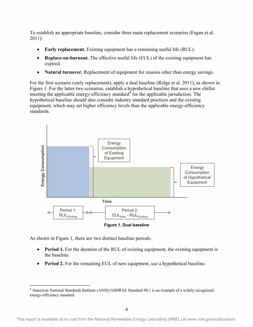
To establish an appropriate baseline, consider three main replacement scenarios (Fagan et al. 2011):
• Early replacement. Existing equipment has a remaining useful life (RUL).
• Replace-on-burnout. The effective useful life (EUL) of the existing equipment has expired.
• Natural turnover. Replacement of equipment for reasons other than energy savings.
For the first scenario (early replacement), apply a dual baseline (Ridge et al. 2011), as shown in Figure 1. For the latter two scenarios, establish a hypothetical baseline that uses a new chiller meeting the applicable energy-efficiency standard4 for the applicable jurisdiction. The hypothetical baseline should also consider industry standard practices and the existing equipment, which may set higher efficiency levels than the applicable energy-efficiency standards.
Figure 1. Dual baseline
As shown in Figure 1, there are two distinct baseline periods:
• Period 1. For the duration of the RUL of existing equipment, the existing equipment is the baseline.
• Period 2. For the remaining EUL of new equipment, use a hypothetical baseline.
4 American National Standards Institute (ANSI)/ASHRAE Standard 90.1 is an example of a widely recognized energy-efficiency standard.
Energy Consumption
of Existing Equipment
Energy Consumption
of Hypothetical Equipment
Period 2:EULNew - RULExisting
Ener
gy C
onsu
mpt
ion
Time
Period 1:RULExisting
5
This report is available at no cost from the National Renewable Energy Laboratory (NREL) at www.nrel.gov/publications.
As available, use the program defined EUL for chiller equipment or consult regional technical reference manuals (TRM); when program or TRM information is not available, use other secondary sources.5 Similarly, use the method defined by the program to determine the RUL of baseline chiller equipment. If this has not been previously established, consider defining RUL as the difference between the EUL and current age of the chiller (or number of years since its last rebuild)6.
5 California’s Database for Energy Efficient Resources suggests an EUL of 20 years for chillers (CPUC 2008). 6 Evaluators should use discretion regarding the scope of the rebuild and how it may impact the RUL of the chiller.
6
This report is available at no cost from the National Renewable Energy Laboratory (NREL) at www.nrel.gov/publications.
4 Measurement and Verification Plan This section contains both recommended approaches to determining chiller energy savings and the directions on how to use the approaches under the following headings:
• Measurement and verification (M&V) method
• Data collection
• Interactive effects
• Detailed procedures
• Regression model direction.
4.1 Measurement and Verification Method This protocol recommends an approach for verifying chiller energy savings that adheres to Option A of the International Performance Measurement and Verification Protocol (IPMVP). Because it is not possible to measure performance data for hypothetical baseline equipment, this protocol recommends Option A (retrofit isolation—key parameter measurement) rather than Option B (retrofit isolation—all parameter measurement).
Key parameters that require measurement include cooling load data and independent variable data, such as outdoor air temperature (OAT). Estimated parameters include manufacturer part-load efficiency data.7
In some cases, metered data may be available directly from the facility’s building automation system (BAS).8 Also, if required, the facility can add control points to the BAS, either as part of the implementation process or specifically for M&V purposes. Where the BAS cannot provide information, the protocol recommends using submeters and data loggers to collect data.
To ensure the M&V method balances the need for accurate energy savings estimates with the need to keep costs in check (relative to project costs and anticipated energy savings), consider two alternate approaches—IPMVP’s Option C and Option D.
• Option C. Consider a whole-facility approach for early replacement projects if metering the required parameters is cost-prohibitive and if the estimated project-level savings are large compared to the random or unexplained energy variations that occur at the whole-facility level.9 This approach is relatively inexpensive because it involves an analysis of facility consumption data. The downside is evaluators cannot perform verification until after collecting a full season or year of reporting period data and monitoring and
7 Even though evaluators can measure efficiency data for the reporting period, under a hypothetical baseline scenario it is generally recommended to use pre- and postinstallation manufacturer efficiency data. This approach provides a more accurate estimate of the change in efficiency in comparison to an approach that uses a combination of measured reporting period efficiency data and manufacturer baseline efficiency data. 8 It is important to ensure qualified service personnel maintain the BAS. Transducers that are out of calibration, or simply broken, could significantly impact M&V results. 9 Typically, savings should exceed 10% of the baseline energy for the facility’s electricity meter to confidently discriminate the savings from the baseline data when the reporting period is shorter than two years (EVO 2012).
7
This report is available at no cost from the National Renewable Energy Laboratory (NREL) at www.nrel.gov/publications.
documenting any changes to the facility’s static factors10 over the course of the measurement period. Also, an analysis of monthly consumption data may be inadequate for estimating peak demand savings; evaluators should investigate whether data from advanced metering infrastructure (e.g., interval meters) is available to increase the accuracy of billing data analyses.
• Option D. Consider a calibrated simulation approach if metering the required parameters is cost-prohibitive and the estimated project-level savings are small compared to the random or unexplained energy variations that occur at the whole-facility level. Undertake calibration in two ways: (1) calibrate the simulation to actual baseline or reporting period consumption data and (2) confirm the reporting period inputs via the BAS front-end system or the chiller control terminal, when possible. 11,12
4.2 Data Collection When using Option A (the preferred approach) to assess chiller measures, the following M&V elements require particular consideration:
• Measurement boundary
• Measurement period and frequency
• Functionality of the measurement equipment
• Savings uncertainty.
4.2.1 Measurement Boundary For all projects, especially those that require metering external to the BAS, it is important to define the measurement boundary. When determining boundaries, consider the location and number of measurement points required as well as the project’s complexity and expected savings:
• A narrow boundary simplifies data measurement (e.g., chiller plant equipment directly affected by the chiller measure), but will require accounting for any variables driving energy use outside the boundary (interactive effects)13
• A wide boundary will minimize interactive effects and increase accuracy. However, since M&V costs may also increase, it is important to ensure the expected increase in the accuracy of the project savings justifies the M&V cost increase.
10 Many factors can affect a facility’s energy consumption even though evaluators do not expect them to change. These factors are known as “static factors” and include the complete collection of facility parameters that are generally expected to remain constant between the baseline and reporting periods. Examples include: building-envelope insulation, space use within a facility, and facility square footage. 11 In many cases, the simulation should represent the entire facility; however, in some cases, depending on the facility’s wiring structure, evaluators can apply a similar approach to building submeters, such as distribution panels that include the affected systems. 12 See the Uniform Methods Project’s Commercial New Construction Protocol for more information on using Option D. 13 Although significant interactive effects are uncommon for chiller measures, there are some scenarios that warrant consideration. See Section 4.3 for further detail.
8
This report is available at no cost from the National Renewable Energy Laboratory (NREL) at www.nrel.gov/publications.
4.2.2 Measurement Period and Frequency Consider these important timing metrics: (1) the measurement period and (2) the measurement frequency. In general:
• Choose the measurement period (the length of the baseline and reporting periods) to capture a full cycle of each operating mode. For example, if a chiller is serving an HVAC load, collect data over the summer, shoulder, and winter seasons (if applicable).
• Choose the measurement frequency (the regularity of measurements during the measurement period) by assessing the type of load:
o Spot measurement. For constant loads (e.g., constant-speed chilled water pumps), measure power briefly, preferably over two or more intervals.
o Short-term measurement. For loads predictably influenced by independent variables (e.g., chiller compressors serving HVAC loads), take short-term consumption measurements over the fullest range of possible independent variable conditions, given M&V project cost and time limitations.
o Continuous measurement. For variable loads (e.g., chiller compressors serving process loads), measure consumption data continuously, or at appropriate discrete intervals, over the entire measurement period.
Section 4.4, Detailed Procedures, provides directions regarding measurement period and frequency for each element of the previously introduced savings equation.
4.2.3 Measurement Equipment When the BAS cannot provide enough information and submeters are necessary to obtain data, use these guidelines to select the appropriate meter:14
• Size the meter for the range of values expected most of the time.
• Select the meter repeatability and accuracy that fits the budget and intended use of the data.
• Install the meter as recommended by the manufacturer.
• Calibrate the meter before it goes into the field and maintain meter calibration, as recommended by the manufacturer. If possible, select a meter with a recommended calibration interval that is longer than the anticipated measurement period.
• If budget allows, consider installing submeters permanently.
If using BAS data, exercise due diligence by determining when the BAS was last calibrated and by checking the accuracy of the BAS measurement points.
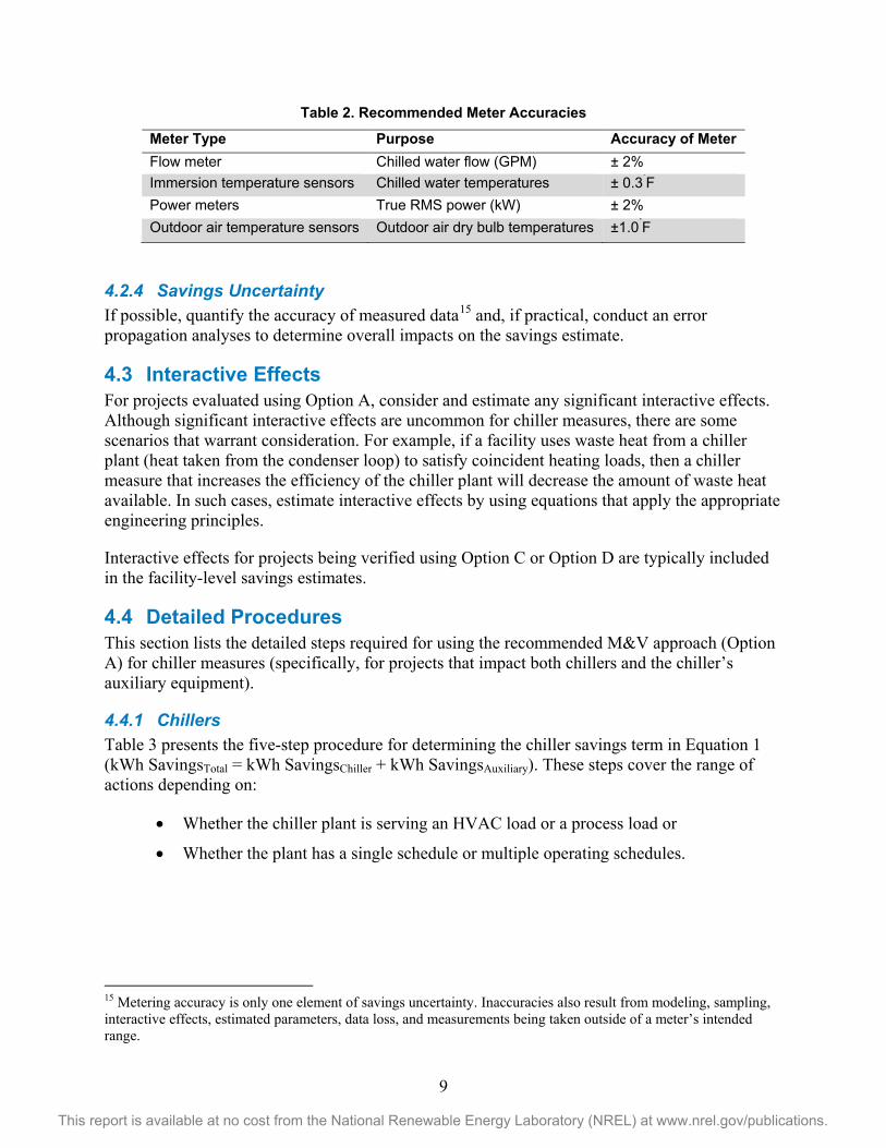
Table 2 lists recommended levels of accuracy for the types of metering equipment used for chiller M&V (US DOE FEMP 2008).
14 Further information on choosing meters can be found in the Uniform Methods Project’s Metering Cross-Cutting Protocols.
9
This report is available at no cost from the National Renewable Energy Laboratory (NREL) at www.nrel.gov/publications.
Table 2. Recommended Meter Accuracies
Meter Type Purpose Accuracy of Meter Flow meter Chilled water flow (GPM) ± 2% Immersion temperature sensors Chilled water temperatures ± 0.3˚F Power meters True RMS power (kW) ± 2% Outdoor air temperature sensors Outdoor air dry bulb temperatures ±1.0˚F
4.2.4 Savings Uncertainty If possible, quantify the accuracy of measured data15 and, if practical, conduct an error propagation analyses to determine overall impacts on the savings estimate.
4.3 Interactive Effects For projects evaluated using Option A, consider and estimate any significant interactive effects. Although significant interactive effects are uncommon for chiller measures, there are some scenarios that warrant consideration. For example, if a facility uses waste heat from a chiller plant (heat taken from the condenser loop) to satisfy coincident heating loads, then a chiller measure that increases the efficiency of the chiller plant will decrease the amount of waste heat available. In such cases, estimate interactive effects by using equations that apply the appropriate engineering principles.
Interactive effects for projects being verified using Option C or Option D are typically included in the facility-level savings estimates.
4.4 Detailed Procedures This section lists the detailed steps required for using the recommended M&V approach (Option A) for chiller measures (specifically, for projects that impact both chillers and the chiller’s auxiliary equipment).
4.4.1 Chillers Table 3 presents the five-step procedure for determining the chiller savings term in Equation 1 (kWh SavingsTotal = kWh SavingsChiller + kWh SavingsAuxiliary). These steps cover the range of actions depending on:
• Whether the chiller plant is serving an HVAC load or a process load or
• Whether the plant has a single schedule or multiple operating schedules.
15 Metering accuracy is only one element of savings uncertainty. Inaccuracies also result from modeling, sampling, interactive effects, estimated parameters, data loss, and measurements being taken outside of a meter’s intended range.
10
This report is available at no cost from the National Renewable Energy Laboratory (NREL) at www.nrel.gov/publications.
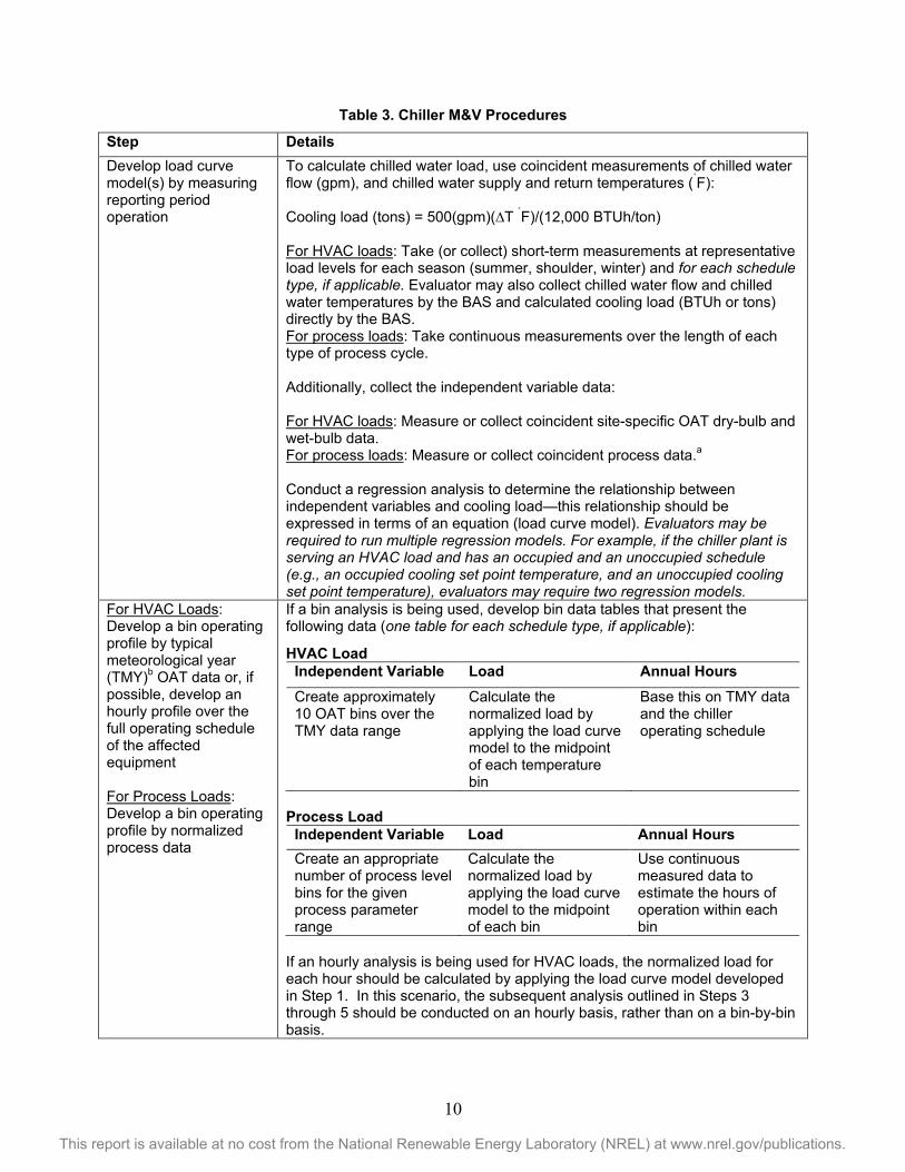
Table 3. Chiller M&V Procedures
Step Details Develop load curve model(s) by measuring reporting period operation
To calculate chilled water load, use coincident measurements of chilled water flow (gpm), and chilled water supply and return temperatures (˚F): Cooling load (tons) = 500(gpm)(∆T ˚F)/(12,000 BTUh/ton) For HVAC loads: Take (or collect) short-term measurements at representative load levels for each season (summer, shoulder, winter) and for each schedule type, if applicable. Evaluator may also collect chilled water flow and chilled water temperatures by the BAS and calculated cooling load (BTUh or tons) directly by the BAS. For process loads: Take continuous measurements over the length of each type of process cycle. Additionally, collect the independent variable data: For HVAC loads: Measure or collect coincident site-specific OAT dry-bulb and wet-bulb data. For process loads: Measure or collect coincident process data.a Conduct a regression analysis to determine the relationship between independent variables and cooling load—this relationship should be expressed in terms of an equation (load curve model). Evaluators may be required to run multiple regression models. For example, if the chiller plant is serving an HVAC load and has an occupied and an unoccupied schedule (e.g., an occupied cooling set point temperature, and an unoccupied cooling set point temperature), evaluators may require two regression models.
For HVAC Loads: Develop a bin operating profile by typical meteorological year (TMY)b OAT data or, if possible, develop an hourly profile over the full operating schedule of the affected equipment For Process Loads: Develop a bin operating profile by normalized process data
If a bin analysis is being used, develop bin data tables that present the following data (one table for each schedule type, if applicable):
HVAC Load Independent Variable Load Annual Hours Create approximately 10 OAT bins over the TMY data range
Calculate the normalized load by applying the load curve model to the midpoint of each temperature bin
Base this on TMY data and the chiller operating schedule
Process Load
Independent Variable Load Annual Hours Create an appropriate number of process level bins for the given process parameter range
Calculate the normalized load by applying the load curve model to the midpoint of each bin
Use continuous measured data to estimate the hours of operation within each bin
If an hourly analysis is being used for HVAC loads, the normalized load for each hour should be calculated by applying the load curve model developed in Step 1. In this scenario, the subsequent analysis outlined in Steps 3 through 5 should be conducted on an hourly basis, rather than on a bin-by-bin basis.
11
This report is available at no cost from the National Renewable Energy Laboratory (NREL) at www.nrel.gov/publications.
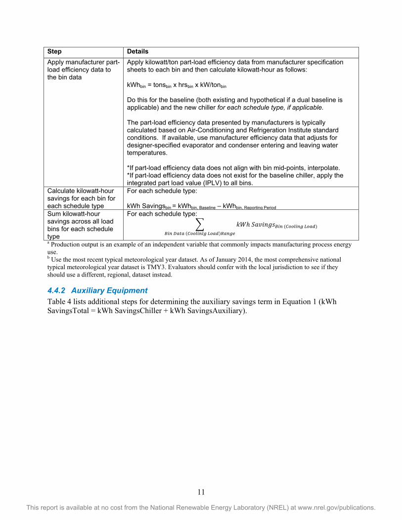
Step Details Apply manufacturer part-load efficiency data to the bin data
Apply kilowatt/ton part-load efficiency data from manufacturer specification sheets to each bin and then calculate kilowatt-hour as follows: kWhbin = tonsbin x hrsbin x kW/tonbin Do this for the baseline (both existing and hypothetical if a dual baseline is applicable) and the new chiller for each schedule type, if applicable. The part-load efficiency data presented by manufacturers is typically calculated based on Air-Conditioning and Refrigeration Institute standard conditions. If available, use manufacturer efficiency data that adjusts for designer-specified evaporator and condenser entering and leaving water temperatures. *If part-load efficiency data does not align with bin mid-points, interpolate. *If part-load efficiency data does not exist for the baseline chiller, apply the integrated part load value (IPLV) to all bins.
Calculate kilowatt-hour savings for each bin for each schedule type
For each schedule type: kWh Savingsbin = kWhbin, Baseline – kWhbin, Reporting Period
Sum kilowatt-hour savings across all load bins for each schedule type
For each schedule type: � 𝑘𝑊ℎ 𝑆𝑎𝑣𝑖𝑛𝑔𝑠𝐵𝑖𝑛 (𝐶𝑜𝑜𝑙𝑖𝑛𝑔 𝐿𝑜𝑎𝑑)
𝐵𝑖𝑛 𝐷𝑎𝑡𝑎 (𝐶𝑜𝑜𝑙𝑖𝑛𝑙𝑔 𝐿𝑜𝑎𝑑)𝑅𝑎𝑛𝑔𝑒
a Production output is an example of an independent variable that commonly impacts manufacturing process energy use. b Use the most recent typical meteorological year dataset. As of January 2014, the most comprehensive national typical meteorological year dataset is TMY3. Evaluators should confer with the local jurisdiction to see if they should use a different, regional, dataset instead. 4.4.2 Auxiliary Equipment Table 4 lists additional steps for determining the auxiliary savings term in Equation 1 (kWh SavingsTotal = kWh SavingsChiller + kWh SavingsAuxiliary).
12
This report is available at no cost from the National Renewable Energy Laboratory (NREL) at www.nrel.gov/publications.
Table 4. Auxiliary Equipment M&V Procedures
Step Details Measure baselinea and reporting period auxiliary demand data
If the energy consumption of auxiliary equipment is constant, take spot measurements on the auxiliary equipment affected by the chiller measure. If consumption of auxiliary equipment is variable and the chiller plant is serving an HVAC load, take short-term measurements at representative load levels for auxiliary equipment affected by the chiller measure. If consumption of auxiliary equipment is variable and the chiller plant is serving a process load, take continuous measurements over the length of each type of process cycle for all auxiliary equipment affected by the chiller measure. If more than one piece of auxiliary equipment is affected, the measurements across affected equipment should be coincident.
Develop bin data and sum the kilowatt-hour savings
Bin baseline and reporting period data using bin profiles established for the chiller (if consumption of auxiliary equipment is constant—as it might likely be for the baseline scenario; kilowatts will be the same for all bins). Calculate kilowatt-hour savings by bin and sum as described in Table 3.
a If auxiliary equipment is replaced as part of a replace-on-burnout or natural turnover project, the building code could require upgrades to the auxiliary equipment. If this is the case, establish a hypothetical baseline for the affected auxiliary equipment. 4.5 Regression Modeling Direction Calculating normalized savings for the majority of projects—whether following the IPMVP’s Option A or Option C—will require the development of a baseline and reporting period regression model.16 Use one of the following three types of analysis methods to create the model:
• Linear regression: For one routinely varying significant parameter (e.g., OAT).17
• Multivariable linear regression: For more than one routinely varying significant parameter (e.g., OAT, process parameter).
• Advanced regression: For a multivariable, nonlinear fit requiring a polynomial or exponential model.18
Develop all models in accordance with common practices and only use them when statistically valid (see Section 4.5.2, Testing Model Validity). If there are no significant independent variables (as would be the case for a constant-process cooling load), evaluators are not required to use a model because the calculated savings are inherently normalized.
16 This could either be a single regression model that uses a dummy variable to differentiate the baseline/reporting period data or two independent models for the baseline and reporting period, respectively. 17 One of the most common linear regression models is the three-parameter change point model. For example, a model that represents cooling electricity consumption will have one regression coefficient that describes non-weather-dependent electricity use, a second regression coefficient that describes the rate of increase of electricity use with increasing temperature, and a third parameter that describes the change point temperature, also known as the balance point temperature, where weather-dependent electricity use begins. 18 Evaluators may need to use advanced regression methods if a chiller plant is providing cooling for manufacturing or industrial processes.
13
This report is available at no cost from the National Renewable Energy Laboratory (NREL) at www.nrel.gov/publications.
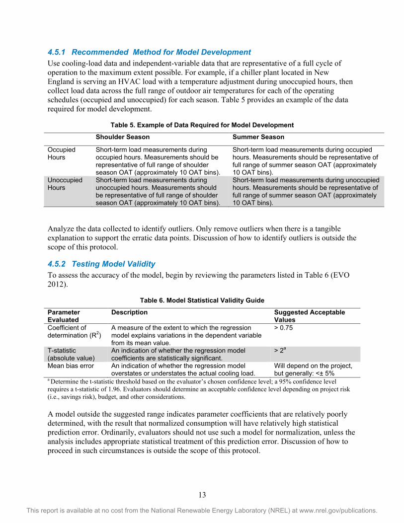
4.5.1 Recommended Method for Model Development Use cooling-load data and independent-variable data that are representative of a full cycle of operation to the maximum extent possible. For example, if a chiller plant located in New England is serving an HVAC load with a temperature adjustment during unoccupied hours, then collect load data across the full range of outdoor air temperatures for each of the operating schedules (occupied and unoccupied) for each season. Table 5 provides an example of the data required for model development.
Table 5. Example of Data Required for Model Development
Shoulder Season Summer Season
Occupied Hours
Short-term load measurements during occupied hours. Measurements should be representative of full range of shoulder season OAT (approximately 10 OAT bins).
Short-term load measurements during occupied hours. Measurements should be representative of full range of summer season OAT (approximately 10 OAT bins).
Unoccupied Hours
Short-term load measurements during unoccupied hours. Measurements should be representative of full range of shoulder season OAT (approximately 10 OAT bins).
Short-term load measurements during unoccupied hours. Measurements should be representative of full range of summer season OAT (approximately 10 OAT bins).
Analyze the data collected to identify outliers. Only remove outliers when there is a tangible explanation to support the erratic data points. Discussion of how to identify outliers is outside the scope of this protocol.
4.5.2 Testing Model Validity To assess the accuracy of the model, begin by reviewing the parameters listed in Table 6 (EVO 2012).
Table 6. Model Statistical Validity Guide
Parameter Evaluated
Description Suggested Acceptable Values
Coefficient of determination (R2)
A measure of the extent to which the regression model explains variations in the dependent variable from its mean value.
> 0.75
T-statistic (absolute value)
An indication of whether the regression model coefficients are statistically significant.
> 2a
Mean bias error An indication of whether the regression model overstates or understates the actual cooling load.
Will depend on the project, but generally: <± 5%
a Determine the t-statistic threshold based on the evaluator’s chosen confidence level; a 95% confidence level requires a t-statistic of 1.96. Evaluators should determine an acceptable confidence level depending on project risk (i.e., savings risk), budget, and other considerations. A model outside the suggested range indicates parameter coefficients that are relatively poorly determined, with the result that normalized consumption will have relatively high statistical prediction error. Ordinarily, evaluators should not use such a model for normalization, unless the analysis includes appropriate statistical treatment of this prediction error. Discussion of how to proceed in such circumstances is outside the scope of this protocol.
14
This report is available at no cost from the National Renewable Energy Laboratory (NREL) at www.nrel.gov/publications.
When possible, attempt to enhance the regression model by:
• Increasing or shifting the measurement period
• Incorporating more data points
• Including independent variables previously unidentified
Also, when assessing model validity, consider the coefficient of variation (CV) of the root mean squared error (RMSE), fractional savings uncertainty, and residual plots. Refer to ASHRAE Guideline 14-2002 and Bonneville Power Administration’s Regression for M&V: Reference Guide for direction on how assess these additional parameters.
15
This report is available at no cost from the National Renewable Energy Laboratory (NREL) at www.nrel.gov/publications.
5 Sample Design Consult the Uniform Methods Project’s Chapter 11: Sample Design Cross-Cutting Protocol for general sampling procedures if the chiller project population is sufficiently large or if the evaluation budget is constrained. Ideally, use stratified sampling to partition chiller projects by facility type, process vs. HVAC load, and/or the magnitude of claimed (ex ante) project savings. Stratification ensures evaluators can confidently extrapolate sample findings to the remaining project population. Regulatory or program administrator specifications typically govern the confidence and precision targets, which will influence sample size.
16
This report is available at no cost from the National Renewable Energy Laboratory (NREL) at www.nrel.gov/publications.
6 Other Evaluation Issues When claiming lifetime and net program chiller measure impacts, consider the following evaluation issues in addition to first-year gross impact findings:
• Net-to-gross estimation
• Early replacement
• Dual baseline realization rates.
6.1 Net-to-Gross Estimation The Uniform Methods Project’s cross-cutting Estimating Net Savings: Common Practices discusses an approach for determining net program impacts at a general level. It is recommended that the collection between gross and net impact results and teams collecting site-specific impact data to ensure there is no double counting of adjustments to impacts at a population level.
6.2 Early Replacement As a supplement to the Uniform Methods Project’s Estimating Net Savings: Common Practices, the evaluator should consider assessing whether early replacement projects were program-induced. If the early replacement was not program-induced, it is appropriate to use a hypothetical baseline rather than a dual baseline.
6.3 Dual-Baseline Realization Rates For program-induced early replacement projects, two different realization rates (evaluated [ex post] gross savings/claimed [ex ante] gross savings) exist over the EUL of the new equipment:
• Period 1 Realization Rate. The realization rate is applicable over the first part of the dual baseline; evaluators should calculate the gross ex post savings using the existing equipment as the baseline.
• Period 2 Realization Rate. The realization rate is applicable over second part of the dual baseline; evaluators should calculate the gross ex post savings using a hypothetical baseline.
Therefore, if reporting life cycle gross impact findings, evaluators need to account for both Period 1 and Period 2 realization rates.
17
This report is available at no cost from the National Renewable Energy Laboratory (NREL) at www.nrel.gov/publications.
References ASHRAE. (2002). Guideline 14-2002: Measurement of Energy and Demand Savings. American Society of Heating, Refrigeration and Air-Conditioning Engineers.
ASHRAE. (2012). 2012 ASHRAE Handbook: HVAC Systems and Equipment. American Society of Heating, Refrigeration and Air-Conditioning Engineers.
CPUC. (2008). Database for Energy Efficiency Resources (DEER). California Public Utilities Commission.
EVO. (January 2012). International Performance Measurement and Verification Protocol – Concepts and Options for Determining Energy and Water Savings Volume 1. Efficiency Valuation Organization.
Fagan, F., Bradley, K., Lutz, A. (2011). Strategies for Improving the Accuracy of Industrial Program Savings Estimates and Increasing Overall Program Influence. Prepared for the International Energy Program Evaluation Conference.
Ridge, R., Jacobs, P., Tress, H., Hall, N., Evans, B. (2011). One Solution to Capturing the Benefits of Early Replacement: When Approximately Correct is Good Enough. Prepared for the International Energy Program Evaluation Conference.
US DOE FEMP. (April 2008). M&V Guidelines: Measurement and Verification for Federal Energy Projects—Version 3.0. U.S. Department of Energy Federal Energy Management Program.
18
This report is available at no cost from the National Renewable Energy Laboratory (NREL) at www.nrel.gov/publications.
Bibliography BPA. (2011). Regression for M&V: Reference Guide. Bonneville Power Administration.
CPUC. (April 2006). California Energy Efficiency Evaluation Protocols: Technical, Methodological, and Reporting Requirements for Evaluation Professionals. California Public Utilities Commission.
Connecticut Light & Power, United Illuminating Company. (2005). UI and CL&P Program Savings Documentation for 2006 Program Year.
Itron, Inc. (February 2010). 2006-2008 Evaluation Report for PG&E Fabrication, Process and Manufacturing Contract Group. Prepared for California Public Utilities Commission.
Jacobson, D., Studer, E. (2007). Lessons Learned from a Decade of Evaluating Customized Commercial and Industrial Efficiency Measures. Prepared for the International Energy Program Evaluation Conference.
NEEP. (May 2010). Regional EM&V Methods and Savings Assumptions Guidelines. Northeast Energy Efficiency Partnerships.
OPA. (March 2011). saveONenergy Retrofit Program Project Measurement and Verification Procedures. Ontario Power Authority.
RLW Analytics, Inc. (October 2008). 2004-2005 Los Angeles County —Internal Services Department / Southern California Edison/Southern California Gas Company Energy Efficiency Partnership Impact Evaluation Study. Prepared for California Public Utilities Commission. Robert Mowris & Associates. (June 2005). Measurement & Verification Load Impact Study for NCPA SB5X Commercial and Industrial HVAC Incentive Programs. Prepared for Northern California Power Agency. Summit Blue Consulting, LLC. (September 2008). APS Measurement, Evaluation & Research (MER) Report—Solutions for Business. Prepared for Arizona Power Service.