Draft version June 11, 2021Typeset using LATEX twocolumn style in AASTeX63

The CHIME Pulsar Project: System Overview

CHIME/Pulsar Collaboration, M. Amiri,1 K. M. Bandura,2, 3 P. J. Boyle,4, 5 C. Brar,4, 5 J.-F. Cliche,4, 5

K. Crowter,1 D. Cubranic,1 P. B. Demorest,6 N. T. Denman,7 M. Dobbs,4, 5 F. Q. Dong,1 M. Fandino,1

E. Fonseca,4, 5 D. C. Good,1 M. Halpern,1 A. S. Hill,8, 9 C. Hofer,1 V. M. Kaspi,4, 5 T. L. Landecker,9

C. Leung,10, 11 H.-H. Lin,12, 13 J. Luo,12 K. W. Masui,10, 11 J. W. McKee,12 J. Mena-Parra,10 B. W. Meyers,1

D. Michilli,4, 5 A. Naidu,4, 5 L. Newburgh,14 C. Ng,15 C. Patel,15, 4 T. Pinsonneault-Marotte,1 S. M. Ransom,16

A. Renard,15 P. Scholz,15 J. R. Shaw,1 A. E. Sikora,4, 5 I. H. Stairs,1 C. M. Tan,4, 5 S. P. Tendulkar,4, 5

I. Tretyakov,15, 17 K. Vanderlinde,18, 15 H. Wang,10, 11 and X. Wang19

1Department of Physics & Astronomy, University of British Columbia, 6224 Agricultural Road, Vancouver, BC V6T 1Z1, Canada2CSEE, West Virginia University, Morgantown, WV 26505, USA

3Center for Gravitational Waves and Cosmology, West Virginia University, Morgantown, WV 26505, USA4Department of Physics, McGill University, 3600 rue University, Montreal, QC H3A 2T8, Canada5McGill Space Institute, McGill University, 3550 rue University, Montreal, QC H3A 2A7, Canada

6National Radio Astronomy Observatory, P.O. Box O, Socorro, NM 87801 USA7Central Development Laboratory, National Radio Astronomy Observatory, 1180 Boxwood Estate Road, Charlottesville, VA USA 229038Department of Computer Science, Math, Physics, and Statistics, University of British Columbia, 3187 University Way, Kelowna, BC

V1V 1V7, Canada9National Research Council Canada, Herzberg Research Centre for Astronomy and Astrophysics, Domionion Radio Astrophysical

Observatory, PO Box 248, Penticton BC V2A 6J9, Canada10MIT Kavli Institute for Astrophysics and Space Research, Massachusetts Institute of Technology, 77 Massachusetts Ave, Cambridge,

MA 02139, USA11Department of Physics, Massachusetts Institute of Technology, 77 Massachusetts Ave, Cambridge, MA 02139, USA

12Canadian Institute for Theoretical Astrophysics, 60 St. George Street, Toronto, ON M5S 3H8, Canada13Max Planck Institute for Radio Astronomy, Auf dem Huegel 69, 53121 Bonn, Germany

14Department of Physics, Yale University, New Haven, CT 06520, USA15Dunlap Institute for Astronomy & Astrophysics, University of Toronto, 50 St. George Street, Toronto, ON M5S 3H4, Canada

16National Radio Astronomy Observatory, 520 Edgemont Rd., Charlottesville, VA 22903, USA17Department of Physics, University of Toronto, Toronto, Ontario, M5S 3H4, Canada

18David A. Dunlap Department of Astronomy & Astrophysics, University of Toronto, 50 St. George Street, Toronto, ON M5S 3H4,Canada

19School of Physics and Astronomy, Sun Yat-sen University, 2 Daxue Road, Zhuhai, China

(Received XXX; Revised YYY; Accepted ZZZ)

ABSTRACT

We present the design, implementation, and performance of the digital pulsar observing system

constructed for the Canadian Hydrogen Intensity Mapping Experiment (CHIME). Using accelerated

computing, this system processes independent, digitally-steered beams formed by the CHIME correla-

tor to simultaneously observe up to 10 radio pulsars and transient sources. Each of these independent

streams are processed by the CHIME/Pulsar backend system which can coherently dedisperse, in real

time, up to dispersion measure values of 2500 pc cm−3. The tracking beams and real-time analysis

system are autonomously controlled by a priority-based algorithm that schedules both known sources

and positions of interest for observation with observing cadences as rapid as one day. Given the distri-

bution of known pulsars and radio-transient sources, and the dynamic scheduling, the CHIME/Pulsar

system can monitor 400–500 positions once per sidereal day and observe most sources with declina-

tions greater than −20◦ once every ∼4 weeks. We also discuss the extensive science program enabled

Corresponding author: A. Naidu

arun.naidu@mail.mcgill.ca

arX

iv:2

008.

0568

1v2

[as

tro-

ph.I

M]

10

Jun

2021

2 CHIME/Pulsar Collaboration et al.

through the current modes of data acquisition for CHIME/Pulsar that centers on timing and searching

experiments.

Keywords: instrumentation: interferometers – methods: observational – radio continuum: general –

pulsars: general – techniques: interferometric – telescopes

1. INTRODUCTION

The Canadian Hydrogen Intensity Mapping Experi-

ment (CHIME1) is a radio interferometer operating in

the 400–800 MHz frequency range, located at the Do-

minion Radio Astrophysical Observatory (DRAO) in

Penticton, British Columbia, Canada. CHIME is a

wide-field transit telescope with no physical-slew ca-

pabilities, with a primary design goal to study dark

energy through the measurement of the evolution of

baryon acoustic oscillations across the redshift range of

0.8 < z < 2.5. This measurement will be accomplished

by mapping neutral-hydrogen emission as a function of

frequency across the entire Northern sky. From initial

conception, it was realized that the CHIME telescope

is also highly suitable for high-cadence observations of

radio pulsars, while later planning and development was

undertaken to enable untargeted searches for fast radio

bursts (FRBs; see e.g. Lorimer et al. 2007; Thornton

et al. 2013; Petroff et al. 2019). To date, several tele-

scope backends have been developed for CHIME that

perform pulsar and FRB observations, as well as very-

long baseline interferometry (VLBI) and forthcoming

measurements of neutral-hydrogen absorption systems

(Yu et al. 2014). In this work, we describe the de-

sign, performance, and motivation of a pulsar-timing

system constructed for CHIME, hereafter referred to as

CHIME/Pulsar.

CHIME and the CHIME/Pulsar system differ

from other radio observatories in two distinct ways:

CHIME/Pulsar observes up to 10 different celestial

positions at any instant in time, capable of acquir-

ing spectro-temporal data in two different acquisition

modes commonly used in pulsar and FRB astronomy;

and CHIME/Pulsar is designed to observe continuously

with the CHIME FX correlator, and commensally with

other CHIME backends. These two capabilities allow

CHIME/Pulsar to observe 400–500 known pulsars per

day, and nearly all known sources in the the CHIME

field of view (i.e., δ > −20◦) within one month. CHIME

therefore acts as an automated, high-cadence observa-

tory for pulsar science.

Until recently, only a small fraction of the ∼2800

known radio pulsars was observed regularly using other

1 https://chime-experiment.ca

radio facilities due to competitive and limited telescope

resources. Nonetheless, high-cadence observations of

many millisecond pulsars (MSPs) have been projected

to: boost sensitivity towards nearby, resolvable sources

of nanohertz-frequency gravitational waves (GWs) emit-

ted from merging galaxies (e.g. Christy et al. 2014); re-

solve abrupt temporal variations in dispersion properties

that reflect a complex interstellar medium (ISM; e.g.,

Lam et al. 2018); and constrain the equation of state of

ultra-dense matter (e.g. Demorest et al. 2010). Further-

more, high precision timing of an array of many stable

MSPs is being used to search for, and directly detect,

the low frequency GW background (e.g. Verbiest et al.

2016; Perera et al. 2019), a concept commonly referred

to as a “pulsar timing array” (PTA).

Renewed and frequent tracking of historically low-

priority sources will likely resolve dynamical processes

affecting pulsar rotation, such as unidentified long-

period orbital motion (Kaplan et al. 2016; Bassa et al.

2016; Antoniadis 2021) and many pulsar “glitches” (e.g.

Espinoza et al. 2011). The CHIME/Pulsar system is

also effective at monitoring sporadically emitting pul-

sars and other transient events that can provide great in-

sight into pulsar emission intermittency and astrophysi-

cal coherent radio emission mechanisms more broadly.

The ability of CHIME/Pulsar to monitor the entire

Northern-hemisphere pulsar population on a regular ba-

sis is therefore expected to yield unprecedented access

to a large number of timing-based phenomena that pre-

viously could not be resolved elsewhere.

A brief introduction to the CHIME/Pulsar project

has been presented by Ng & CHIME/Pulsar Collab-

oration (2017). Here we provide a more detailed

overview of the CHIME/Pulsar system, its placement

within the CHIME infrastructure, the performance of

CHIME/Pulsar, and science topics to be addressed with

the CHIME/Pulsar system. In Section 2, we describe

the hardware components of the CHIME instruments

and the pulsar-timing backend. In Section 3, we pro-

vide an overview of the software suite developed to make

pulsar-timing measurements possible with CHIME. In

Section 4, we outline the current performance of the

CHIME/Pulsar system and provide a sample of pre-

liminary results in demonstration of CHIME’s capa-

bilities as a pulsar-timing observatory. In Section 5,

we discuss various scientific opportunities enabled by

The CHIME Pulsar Project: System Overview 3

the CHIME/Pulsar system. Finally, we summarize this

work and its anticipated science outcomes in Section 6.

2. HARDWARE

CHIME consists of 1024 dual-polarization radio-

frequency inputs coupled to a correlator and then sev-

eral independent backend digital instruments. Here we

briefly describe the major signal-chain components rel-

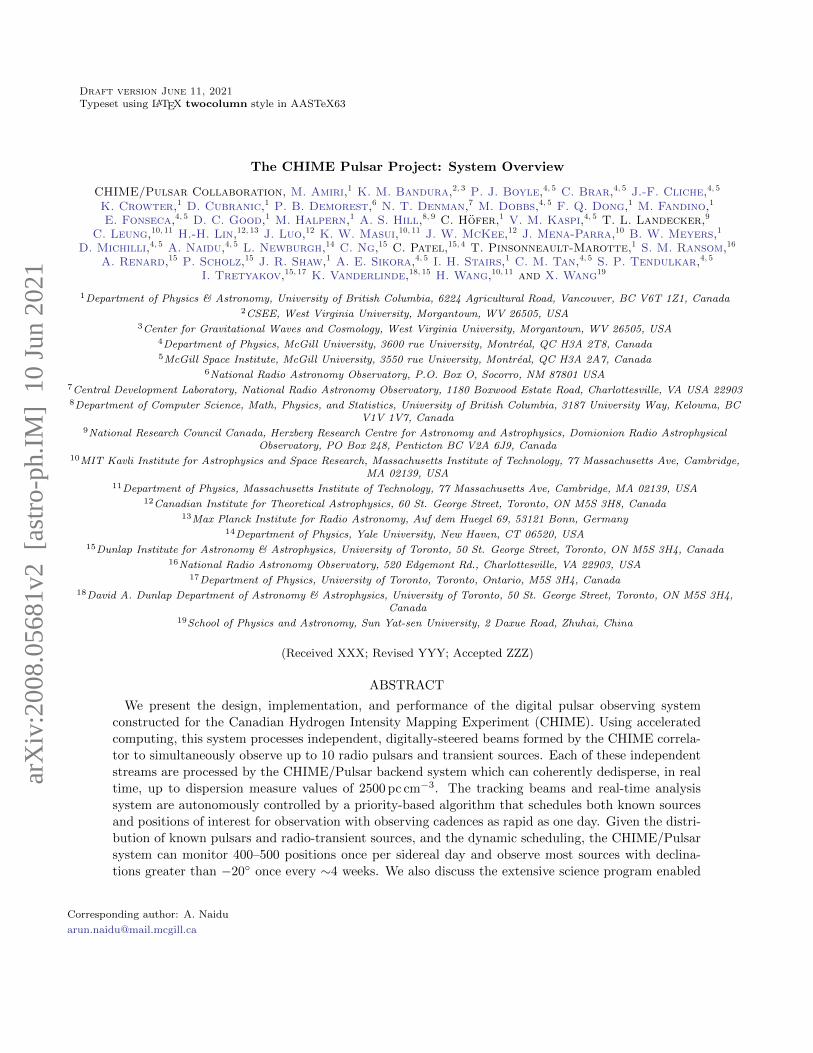
evant to the CHIME/Pulsar project. See Figure 1 for a

schematic diagram of the signal chain from the receivers

to the CHIME/Pulsar backend.

F-Engine

X-Engine

F-Engine

X-Engine

512dual-polinputs6.5Tbps

512dual-polinputs6.5Tbps

NexusSwitchesOtherscienceprojects(e.g.CHIME/VLBI,

CHIME/FRB)10independenttrackingbeams

1024frequencychannels2.56-μstimesampling

6.4Gbps

Pulsarcomputenode(x10)

LocalArchiver

CHIME/Pulsar

Analoguesignalchain

Digitizationandchannelization

GPUcorrelatorandbeamformer

Figure 1. Schematic of the CHIME telescope signal path.The telescope structure (four cylinders, here black arcs), thecorrelator (F- and X-Engines), and the CHIME/Pulsar back-end are shown. The dashed black lines represent coaxial ca-bles carrying the analogue signal from the 256 feeds on eachcylinder to the F-Engines in the East/West receiver enclo-sures, situated below the telescope. The total input datarate into the F-Engine is 13 Tbps. The solid black lines de-pict digitized data carried through copper and/or fiber-opticcables. Networking devices between the F- and X-Enginesare not shown. The X-Engine (GPU-based correlation andbeamforming) is housed in two shipping containers adjacentto the cylinders. The CHIME/Pulsar backend (shaded red)is housed in a shielded room in the DRAO building. Thedata rate into the CHIME/Pulsar backend is 6.4 Gbps.

2.1. Telescope Structure and Receiver

The CHIME telescope consists of four 5-m focal length

parabolic cylinders that are 20 m wide and 100 m long.

The cylinders are oriented North-South, each mounted

with 256 dual-polarization ’cloverleaf’ antennas (Deng

& Campbell-Wilson 2014) placed 30 cm apart below a

68 cm-wide groundplane at the parabolic focus. Two

low noise amplifiers are coupled directly to each an-

tenna. These are coupled via 60 m of low-loss coaxial

cables to custom band-defining filter-amplifiers located

in a radio-frequency shielded room containing analog-

to-digital converters and the frequency channelization

portion of the CHIME correlator. Basic telescope prop-

erties are given in Table 1.

Table 1. Telescope specifications.

Field of view 120◦ (N-S)

1.3-2.5◦ (E-W)

Receiver noise temperature ∼50 K (nominal)

Frequency range 400–800 MHz

Polarization basis orthogonal linear

Telescope longitude −119◦37′25.238′′

Telescope latitude 49◦19′14.553′′

Telescope elevationa 547.918 m

aAbove the GRS 80 ellipsoid.

2.2. FX Correlator

CHIME employs a hybrid FX correlator that consists

of custom-built electronics and adapted commodity pro-

cessing units. The first stage, known as the F-Engine,

is responsible for signal digitization and frequency sepa-

ration, while the second stage, X-Engine, is responsible

for spatial correlation and beamforming.

2.2.1. F-Engine: Digitization and Channelization

The amplified input signals are digitized and sepa-

rated into 1024 frequency channels, resulting in a spec-

tral resolution of 390 kHz, by the F-Engine system. The

details of the F-Engine are presented in Bandura et al.

(2016) and are discussed further in CHIME/FRB Col-

laboration et al. (2018). In summary, the F-Engine con-

sists of 128 “ICE” FPGA-based motherboards where the

signals from the 1024 dual-polarization receivers are dig-

itized at 800 million samples per second with 8-bit preci-

sion. The baseband streams are channelized by a 4-tap

polyphase filterbank into 1024 frequency channels. The

positive frequency spectra of these channelized data are

rounded to (4+4)-bit complex numbers after applying a

programmable gain and phase offset, which halves the

input data rate of 13.1 Tbps to 6.5 Tbps. The complex-

voltage data are further re-organized to form 1024 data

4 CHIME/Pulsar Collaboration et al.

streams, which are transmitted via fibre-optic connec-

tion to the next processing stage.

2.2.2. X-Engine: GPU Correlator and Beamformer

The CHIME correlator X-Engine is a computing clus-

ter consisting of 256 nodes hosting a total of 512 dual-

chip AMD FirePro 9300 X2 graphics processing units

(GPUs). These nodes are divided between two emission-

shielded shipping containers located on the east side of

the CHIME reflectors. Each X-Engine node processes

four frequency channels – one frequency per GPU chip

– for each of the 1024 dual-polarization receiver inputs.

A set of GPU kernels process the input data to manipu-

late the CHIME baseband into a variety of data products

required by downstream backends. The kernel used by

CHIME/Pulsar system is discussed in Section 3.1. The

X-Engine data products are exported from the nodes

over Gigabit Ethernet (GbE) to a set of commercially-

available network switches, and then to various backend

systems. A full description of the CHIME X-Engine and

its capabilities is given by Denman et al. (2020).

2.3. CHIME/Pulsar Backend

The CHIME/Pulsar backend consists of ten indepen-

dent compute nodes that are connected directly to the

CHIME correlator through a series of network switches.

Each compute node consists of a Supermicro mother-

board, an Intel Xeon E5-1650 central processing unit

(CPU), 128 GB of RAM, and a solid-state drive (SSD).

Data are received through a 10-Gbps Intel Network In-

terface Controller (NIC) and is temporarily buffered in

RAM before being processed through an FFT-based co-

herent dedispersion algorithm on a single, liquid-cooled

NVIDIA Titan X GPU. The resulting data are tem-

porarily stored and further processed on a local, 60-TB

data archiver.

2.4. Local Data-archiving Server

The CHIME/Pulsar backend ultimately writes a va-

riety of data products with variable file sizes several

hundred times every sidereal day, at a time-averaged

rate of 67 Mbps. In order to handle the output data

rate, we built a local data-archive server using compo-

nents similar to the hardware described above. The

archiving server employs two redundant arrays of in-

dependent disks (RAIDs) for secure, short-term stor-

age of CHIME/Pulsar data products. This short-term

data archive can accommodate several months of con-

tinuous typical data acquisition, and is sufficient in the

event that higher data-rate modes (see Section 3.3) be-

come emphasized for a moderate time span. These data

are eventually transferred offsite via ground shipment

of physical hard drives to CHIME/Pulsar institutions

for uploading to multi-purpose computing facilities for

offline processing and long-term preservation. The pri-

mary long-term data archiving occurs on the Cedar clus-

ter of Compute Canada2.

3. SOFTWARE

Here we describe the suite of software tools we have de-

veloped and implemented for rendering sky signals from

the FX correlator into useful CHIME/Pulsar data prod-

ucts. Salient details of the CHIME/Pulsar backend out-

put are given in Table 2.

3.1. Beamforming and Calibration

We digitally form 10 dual-polarization tied-array

beams within the X-Engine by summing all 1024 in-

puts phased to specified celestial coordinates. The 10

independent beams allow for tracking of 10 different sky

positions simultaneously within the primary beam of

CHIME. The re-pointing of each beam is performed over

the network using the Representational State Transfer

(REST) application programming interface, and typi-

cally occurs within milliseconds of command execution.

The complex gain calibration (amplitude and phase)

of the input data is achieved via point-source calibration

with bright continuum sources such as Cas A, Cyg A,

and Tau A (CHIME Collaboration et al., in prep.). Dur-

ing a bright continuum source transit, the visibility ma-

trix for CHIME is treated as approximately the product

of the complex gain and sky signal (as viewed through

the beam response function). In this limit, computing

an eigendecomposition of the visibility matrix allows

us to determine the complex gain for each antenna at

each frequency channel in the direction of the calibra-

tor source. The eigenvectors corresponding to the two

largest eigenvalues represent the complex gains for the

X and Y polarizations of each input. After determining

the eigenvectors, we also remove known interferometric

phase based on the physical separation of the antennas

by a process known as fringe-stopping (e.g. Thompson

et al. 2001).

As part of the calibration process, data from poorly

behaving antennas and contaminated frequencies are

masked. A static list of inputs which are known to be

malfunctioning are removed and this list is updated on

a daily basis. Calibration solutions with more than 5%

of inputs deemed bad are flagged as poor quality, and

the most recent, preceding solutions deemed adequate

are instead used until the next calibrator transit oc-

curs. While radio frequency interference (RFI) excision

2 https://www.computecanada.ca

The CHIME Pulsar Project: System Overview 5

Table 2. CHIME/Pulsar data specifications.

Number of tied-array beams 10

Beam width (FWHM) ∼0.5◦ (at 400 MHz)

∼0.25◦ (at 800 MHz)

Number of spectral channels 1024

Frequency resolution 390.625 kHz

Time resolution 2.56µs (baseband)

327.68µs (output filterbank)

Output data bit depth 8

Number of profile binsa 256/512/1024/2048 (fold-mode)

Output polarization state Full Stokes (fold-mode)

Total intensity (filterbank)

X, Y (baseband)

Pulsar data output rateb 67 Mbps

aConfigurable options set when scheduling observations.

bTime-averaged over a typical observing day.

in CHIME data can be a serious challenge, some chan-

nels are known to always be contaminated, and these

channels are masked in the calibration solutions.

During the “pre-commissioning” period of CHIME op-

erations (before August 2018), phase-only calibration

was computed every few days. Since September 2018,

daily amplitude and phase calibration solutions have

been calculated.

3.2. Data packet format, transfer and assembly

For each X-Engine GPU node, the resulting beam-

formed data from each of the four processed frequency

channels are scaled down, encoded into (4+4)-bit com-

plex numbers, and packetized in VLBI Data Interchange

Format (VDIF)3. Each individual packet consists of 625

samples of one of the two polarizations for each of the

four frequency channels and a VDIF header of 32 bytes,

resulting in a total packet size of 5032 bytes. The cor-

responding pulsar data rate on each FX-correlator node

for all 10 beams is 0.2516 Gbps, with a total network

load of ∼64 Gbps for all pulsar beams. Each individual

pulsar-backend node receives ∼6.4 Gbps of data from

the correlator in the form of User Datagram Protocol

(UDP) packets. The incoming data rate to each pul-

sar nodes corresponds to 1.6 × 105 packets per second.

We have optimized our network-capture algorithms in

order to properly receive packets with negligible packet

loss4. The received packets are assembled and written

to memory in preparation of further processing.

3 https://vlbi.org/vlbi-standards/vdif4 The details about the optimizations employed are beyond the

scope of this paper, but available upon request.

3.3. Data processing

The main purpose of the CHIME/Pulsar system is

to autonomously monitor radio pulsars with regular ca-

dence. The beamformed dual-polarization timeseries are

coherently dedispersed and processed to form the data

product defined by the scheduled observation configu-

ration. Most observations occur in “fold mode,” where

the dedispersed baseband data are manipulated to yield

time-averaged pulse profiles for all 1024 frequency chan-

nels over a specified integration time, using a set of pul-

sar rotation parameters for coherent averaging of the sig-

nal. In most cases, the number of profile phase bins for a

given fold-mode observation is 256, although this num-

ber is nominally defined by the science case and, there-

fore, dictated by the scheduling process. By default,

10-second integrations are formed for all fold-mode ob-

servations, although this could in principle be adjustedon a per-pulsar basis. When desired, observations may

also be conducted in “filterbank mode,” where the dedis-

persed baseband timeseries are converted into a Stokes-

I data stream that is then downsampled in time. In

special circumstances, it is scientifically worthwhile to

directly record beamformed baseband data for specific

pulsars and FRBs of interest. We have developed the ap-

propriate software capabilities to enable all three types

of observation with the CHIME/Pulsar system. The

basic output data specifications of the CHIME/Pulsar

system are given in Table 2.

3.3.1. Fold mode

For fold-mode observations, the CHIME/Pulsar back-

end uses the “Digital Signal Processing for Pulsars”

6 CHIME/Pulsar Collaboration et al.

NexusSwitch

UDPstream6.4Gbps

4+4bitencoding

Pulsarnode

NetworkCapture

PacketAssem

bly

PSRDADABuffer&

decodeto8+8bit

Datarearrangment DSPSR

Convolution&Dedispersion

Fold

Integration

Writetodisk

Figure 2. A schematic illustrating the various operations on the data streams from the correlator in fold mode, with colorsdenoting frequency channels. The unordered UDP packets from the correlator are routed to the specified pulsar node wherethe data are organized in the assembler stage which involves both network capture and packet assembly. The assembled data,reordered into a polarization-frequency-time series in order of increasing index variation, are then passed on to the DSPSRprocess using PSRDADA buffers.

(DSPSR) suite5, an open source GPU-based library (van

Straten & Bailes 2011). Written in C++ and CUDA6,

DSPSR is a high performance, general-purpose tool for

high-time-resolution radio pulsar studies using acceler-

ated computing. DSPSR is used in many astrophysical

applications (e.g. Karuppusamy et al. 2012; Martinez

et al. 2015; Price et al. 2016) and is extensively used as

a part of real-time processing instrumentation for vari-

ous telescopes around the world.

DSPSR has the ability to read from and write to data

buffers created using the PSRDADA library7. PSR-

DADA is an open source software that allows the cre-

ation of flexible and well managed ring buffers, with

a variety of applications for piping data from process

to ring buffer, and vice versa. In addition to enabling

transfer of data between processes, PSRDADA provides

various utilities to manage data within the ring buffer

itself.

For fold-mode observations, the incoming data

streams from the CHIME X-Engine are sorted and ar-

ranged as a polarization-frequency-time series prior to

entering the real-time processing stage. The assembled

data are then passed onto the DSPSR process using

PSRDADA buffers. Even though it has the ability to

accept data with (4+4)-bit encoding, DSPSR runs sig-

nificantly faster when instead receiving data with (8+8)-

bit encoding. We have thus modified the PSRDADA

software to convert data to (8+8)-bit encoding before

passing them to DSPSR in order to circumvent this is-

5 http://dspsr.sourceforge.net6 https://developer.nvidia.com/cuda-zone7 http://psrdada.sourceforge.net

sue. Once the data are passed into the DSPSR GPU

buffers, DSPSR executes several kernels that perform

coherent dedispersion and timing-model folding of the

data before writing to disk. A schematic of the pro-

cessing chain for fold-mode observations is presented in

Figure 2.

Output fold-mode data products are written to

structured files (“archives”) that are readable by the

PSRCHIVE software suite8 (Hotan et al. 2004; van

Straten et al. 2012) for offline processing and analy-

sis. An example of the CHIME/Pulsar system fold-mode

data from an observation of PSR B1937+21 is given in

Figure 3.

3.3.2. Filterbank mode

The CHIME/FRB system is discovering many repeat-

ing FRBs (CHIME/FRB Collaboration et al. 2019a,b;

Fonseca et al. 2020), as well as single pulses from un-

known radio pulsars and “rotating radio transients”

(RRATs; McLaughlin et al. 2006). Some fraction of

the CHIME/Pulsar observing time is thus expected

to be used for follow-up observations of these sources.

To observe repeating FRB sources, the pulsar backend

must be able to record coherently dedispersed high-time-

resolution filterbank data. Since these extragalactic

sources are known to have DMs upwards of 1000 pc cm−3

it is also essential that the backend can support such DM

ranges.

The readily available DSPSR filterbank module digifil

cannot support real-time performance at such large DMs

at the CHIME operating frequency range. To overcome

8 http://psrchive.sourceforge.net

The CHIME Pulsar Project: System Overview 7

0.0

0.5

1.0In

tens

ity(a

rb. u

nits

)PSR B1937+21

0 0.2 0.4 0.6 0.8 1Phase

800

700

600

500

400

Freq

uenc

y (M

Hz)

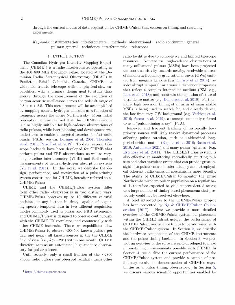
Figure 3. A fold-mode observation of PSR B1937+21. Thebottom panel is the phase versus frequency (waterfall) plot,and the top panel is the mean intensity after summing all fre-quency channels (i.e. the integrated pulse profile). There isclear evidence of pulse broadening due to interstellar scatter-ing visible in the folded profile and as a function of frequencyacross the 400 MHz bandwidth.

this, we have developed a new codebase for the filterbank

mode with the ability to dedisperse incoming data to a

maximum DM of 3300 pc cm−3 in real-time based on

work by Naidu et al. (2015). The significant change in

our implementation is the input data format. Based on

benchmark tests on FFT performance, the efficiency of

the GPUs can be improved by a factor of five if the input

data format is changed from polarization-frequency-time

series to polarization-time-frequency series as shown in

Figure 4.

The received UDP packets are arranged into a

polarization-time-frequency series and are passed on to

the GPU for coherent dedispersion at a user-specified

DM. This dedispersed data are then passed on to the

CPU for downsampling, and then manipulated into a

community-established filterbank format before writing

to disk. All the code for the CPU processes after GPU

kernel execution are written in Intel AVX2 instrinsics.

3.4. Scheduler and web monitors

An automated scheduler is necessary to make maxi-

mal use of the continuous operation of CHIME for pul-

sar observations. The transit nature of the telescope

means that sources are set to be observed only when

they are within 1.75◦ of the meridian. This results in

certain parts of the sky having more sources than the

number of available beams. To address this, we have

developed a probabilistic scheduling algorithm that em-

ploys user-defined weights to prioritize certain sources,

or positions of interest, over others. This priority sys-

tem is used to resolve scheduling conflicts. There are five

base weight values, where the highest weight is assigned

to MSPs currently used in a PTA for gravitational-wave

detection, as well as other interesting pulsars (e.g., rel-

ativistic pulsar-binary systems) such that they will be

observed every day. The remaining four weighting val-

ues are defined such that each additional tier has twice

the weight of the previous tier. There is also a feedback

mechanism that reduces the priority associated with a

source (as long as it is not assigned the highest priority

level) based on the number of days it has been observed

over the previous 14 days. The weight of a previously

scheduled source will be reduced by a factor equivalent

to the number of days observed over the period.

The scheduler adds the next source to the schedule

through an iterative process. It looks for sources whose

transit time began within 7 minutes of the end of the

transit time of the previous source for each one of the ten

beams. In cases where two or more sources fall within

the time-frame, the scheduler will automatically select

the source with a weight that corresponds to being ob-

served daily and starting time of transit being closest

to the end of the transit time of the previous source.

If none of the sources have such weighting, each source

will be given a probability equivalent to its weighting

divided by the weighting of all sources in conflict anda source will be randomly selected with the determined

probabilities.

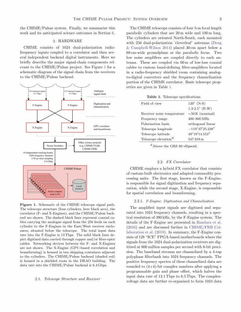
In order to evaluate the effectiveness of the sched-

uler, we examined the number of times each source is

scheduled over a 60-day period. Figure 5 shows the

histograms of sources and how often they are sched-

uled. We found that when the telescope is not transit-

ing the Galactic plane, the scheduler is highly effective

in cycling through all sources, with more than half of

the sources being observed on near-daily cadence (i.e.,

scheduled > 30 times over 60 days), with only about

10 of the 559 sources having a cadence of 2 weeks or

more (i.e., scheduled < 4 times over 60 days). On the

more crowded field of RAs between 18-20 hours, sources

on average will have a longer cadence, with less than

20 sources scheduled with near-daily cadence and about

8 CHIME/Pulsar Collaboration et al.

NexusSwitch

UDPstream6.4Gbps

4+4bitencoding

Pulsarnode

NetworkCapture

PacketAssem

bly

Filterbankpipeline

Convolution&Dedispersion

Integration

Writetodisk

Datarearrangment

Rearrange

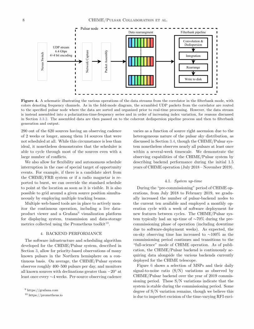
Figure 4. A schematic illustrating the various operations of the data streams from the correlator in the filterbank mode, withcolors denoting frequency channels. As in the fold-mode diagram, the scrambled UDP packets from the correlator are routedto the specified pulsar node where the data are sorted and organized prior to real-time processing. However, the data streamis instead assembled into a polarization-time-frequency series and in order of increasing index variation, for reasons discussedin Section 3.3.2. The assembled data are then passed on to the coherent dedispersion pipeline process and then to filterbankgeneration and output.

290 out of the 620 sources having an observing cadence

of 2 weeks or longer, among them 14 sources that were

not scheduled at all. While this circumstance is less than

ideal, it nonetheless demonstrates that the scheduler is

able to cycle through most of the sources even with a

large number of conflicts.

We also allow for flexibility and autonomous schedule

interruption in the case of special target of opportunity

events. For example, if there is a candidate alert from

the CHIME/FRB system or if a radio magnetar is re-

ported to burst, we can override the standard schedule

to point at the location as soon as it is visible. It is also

possible to grid around a given source position simulta-

neously by employing multiple tracking beams.

Multiple web-based tools are in place to actively mon-

itor the continuous operation, including a live data-

product viewer and a Grafana9 visualization platform

for displaying system, transmission and data-storage

metrics collected using the Prometheus toolkit10.

4. BACKEND PERFORMANCE

The software infrastructure and scheduling algorithm

developed for the CHIME/Pulsar system, described in

Section 3, allow for priority-based observations of many

known pulsars in the Northern hemisphere on a con-

tinuous basis. On average, the CHIME/Pulsar system

observes roughly 400–500 pulsars per day, and monitors

all known sources with declinations greater than −20◦ at

least once every ∼4 weeks. Per-source observing cadence

9 https://grafana.com10 https://prometheus.io

varies as a function of source right ascension due to the

heterogeneous nature of the pulsar sky distribution, as

discussed in Section 3.4, though the CHIME/Pulsar sys-

tem nonetheless observes nearly all pulsars at least once

within a several-week timescale. We demonstrate the

observing capabilities of the CHIME/Pulsar system by

describing backend performance during the initial 1.5

years of CHIME operation (July 2018 – November 2019).

4.1. System up-time

During the “pre-commissioning” period of CHIME op-

erations, from July 2018 to February 2019, we gradu-

ally increased the number of pulsar-backend nodes to

the current ten available and employed a monthly op-

eration cycle with a week of software deployment for

new features between cycles. The CHIME/Pulsar sys-

tem typically had an up-time of ∼70% during the pre-

commissioning phase of operation (including downtime

due to software-deployment weeks). As expected, the

on-sky observing time has increased to ∼100% as the

commissioning period continues and transitions to the

“full-science” mode of CHIME operation. As of publi-

cation, the CHIME/Pulsar backend is continuously ac-

quiring data alongside the various backends currently

deployed for the CHIME telescope.

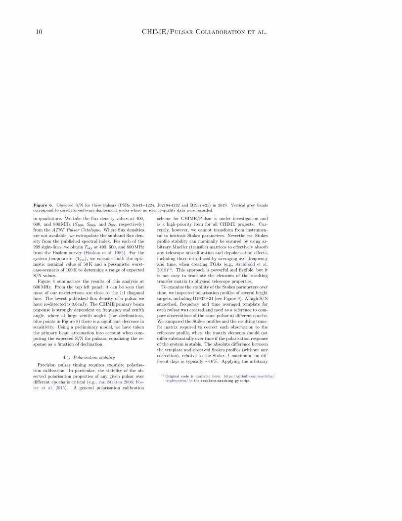
Figure 6 shows a selection of MSPs and their daily

signal-to-noise ratio (S/N) variations as observed by

CHIME/Pulsar backend over the year of 2019 commis-

sioning period. These S/N variations indicate that the

system is stable during the commissioning period. Some

degree of S/N variation remains, though we believe this

is due to imperfect excision of the time-varying RFI envi-

The CHIME Pulsar Project: System Overview 9

Figure 5. Histograms showing the rate that each source isobserved over a period of 60 days, for sources located at RightAscensions (RAs) of between 18-20 and for those outside ofthe RA range. The histograms is binned in units of two,starting with the first bar representing number of sourcesscheduled for either 1 or 2 times over the past 2 months.The number of sources available for each RA range and thenumber of sources not scheduled over the 60-day period areindicated on the plots.

ronment, imperfections in the calibration solutions, and

potentially scintillation effects towards low-DM pulsars.

4.2. Radio frequency interference mitigation

Frequency channels affected by bright RFI (no-

tably the LTE cellular network band between ∼730-

755 MHz and several digital television bands between

500-600 MHz) are identified from the amplitude and

phase calibration solutions provided for each antenna

and frequency channel (see Section 3.1). Since these so-

lutions are calculated and applied on a daily basis, the

particular frequency channels that are masked can vary

on similar timescales, but the RFI environment is gen-

erally stable.

The bulk of RFI excision occurs during post-

processing (e.g., while analyzing the folded or filter-

bank data products). A large fraction of the corrupted

data can be removed by masking an empirically con-

structed list of frequency channels where RFI is persis-

tent (approximately 15% of the band). This corrupted

channel mask can in principle also be combined with

the calibration-based mask applied in the beamforming

stage. More refined RFI excision can be attained by

using techniques available in standard pulsar process-

ing software packages, e.g., PSRCHIVE or PRESTO

(Ransom 2011), but is left to user discretion. For ex-

ample, in Figure 7 we have excised RFI using both the

persistent corrupted channel mask and a method based

on RFI cleaning utilities from the CoastGuard software

suite (Lazarus et al. 2016), where several robust sta-

tistical quantities on a per channel, per subintegration

basis are evaluated to determine whether samples are

corrupted11. Typically, we mask ∼25% of the 1024

frequency channels, yielding ∼300 MHz of usable band-

width spread non-contiguously across the full 400 MHz

observing band. As our understanding of the system

and the RFI environment evolves, these will be tuned to

improve sensitivity.

4.3. Sensitivity

CHIME is nominally capable of observing all known

pulsars down to a declination of ∼ −20◦. To date, we

have re-detected over ∼500 known pulsars with pre-

commissioning CHIME/Pulsar observations. Out of

these ∼500 observable sources, 209 pulsars have pub-

lished flux densities at 600 MHz in the ATNF Pul-

sar Catalogue12 (Manchester et al. 2005). For these

pulsars, we can compare their detected average S/N

with the expected value to assess the sensitivity of the

CHIME/Pulsar system.

We calculate the expected S/N for each pulsar using

the radiometer equation. Many pulsars have steep spec-

tral indices, and the sky temperature (Tsky) will vary

significantly across the 400 MHz bandwidth. Therefore,

in the estimation of the expected S/N, we separately

consider three subbands and sum the three S/N values

11 The exact version of the modified software used here can be foundat https://github.com/bwmeyers/iterative cleaner/tree/v0.9

12 http://www.atnf.csiro.au/people/pulsar/psrcat

10 CHIME/Pulsar Collaboration et al.

58504 58564 58624 58684 58744 58804MJD

101

102

Fold

ed S

/N in

10

min

B1937+21J0218+4232J1643-1224

2019-01-21 2019-03-22 2019-05-21 2019-07-20 2019-09-18 2019-11-17

Figure 6. Observed S/N for three pulsars (PSRs J1643−1224, J0218+4232 and B1937+21) in 2019. Vertical grey bandscorrespond to correlator-software deployment weeks where no science-quality data were recorded.

in quadrature. We take the flux density values at 400,

600, and 800 MHz (S400, S600, and S800 respectively)

from the ATNF Pulsar Catalogue. Where flux densities

are not available, we extrapolate the subband flux den-

sity from the published spectral index. For each of the

209 sight-lines, we obtain Tsky at 400, 600, and 800 MHz

from the Haslam survey (Haslam et al. 1982). For the

system temperature (Tsys), we consider both the opti-

mistic nominal value of 50 K and a pessimistic worst-

case-scenario of 100 K to determine a range of expected

S/N values.

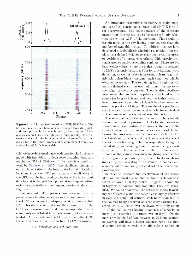
Figure 8 summarizes the results of this analysis at

600 MHz. From the top left panel, it can be seen that

most of our re-detections are close to the 1:1 diagonal

line. The lowest published flux density of a pulsar we

have re-detected is 0.6 mJy. The CHIME primary beam

response is strongly dependent on frequency and zenith

angle, where at large zenith angles (low declinations,

blue points in Figure 8) there is a significant decrease in

sensitivity. Using a preliminary model, we have taken

the primary beam attenuation into account when com-

puting the expected S/N for pulsars, equalizing the re-

sponse as a function of declination.

4.4. Polarisation stability

Precision pulsar timing requires exquisite polarisa-

tion calibration. In particular, the stability of the ob-

served polarisation properties of any given pulsar over

different epochs is critical (e.g., van Straten 2006; Fos-

ter et al. 2015). A general polarisation calibration

scheme for CHIME/Pulsar is under investigation and

is a high-priority item for all CHIME projects. Cur-

rently, however, we cannot transform from instrumen-

tal to intrinsic Stokes parameters. Nevertheless, Stokes

profile stability can nominally be ensured by using ar-

bitrary Mueller (transfer) matrices to effectively absorb

any telescope miscalibration and depolarisation effects,

including those introduced by averaging over frequency

and time, when creating TOAs (e.g., Archibald et al.

2018)13. This approach is powerful and flexible, but it

is not easy to translate the elements of the resulting

transfer matrix to physical telescope properties.

To examine the stability of the Stokes parameters over

time, we inspected polarisation profiles of several bright

targets, including B1937+21 (see Figure 9). A high-S/N

smoothed, frequency and time averaged template for

each pulsar was created and used as a reference to com-

pare observations of the same pulsar at different epochs.

We compared the Stokes profiles and the resulting trans-

fer matrix required to correct each observation to the

reference profile, where the matrix elements should not

differ substantially over time if the polarisation response

of the system is stable. The absolute difference between

the template and observed Stokes profiles (without any

correction), relative to the Stokes I maximum, on dif-

ferent days is typically ∼10%. Applying the arbitrary

13 Original code is available here: https://github.com/aarchiba/triplesystem/ in the template matching.py script.

The CHIME Pulsar Project: System Overview 11

0 50 100 150Day

800

700

600

500

400

Freq

uenc

y (M

Hz)

PSR B0450-18

0.0

0.2

0.4

0.6

0.8

1.0

Frac

tion

of d

ata

flagg

ed

0 20 40 60 80Day

800

700

600

500

400

Freq

uenc

y (M

Hz)

PSR B1900+01

0.0

0.2

0.4

0.6

0.8

1.0

Frac

tion

of d

ata

flagg

ed

0 50 100 150Day

800

700

600

500

400

Freq

uenc

y (M

Hz)

PSR B1937+21

0.0

0.2

0.4

0.6

0.8

1.0

Frac

tion

of d

ata

flagg

ed

0 20 40 60Day

800

700

600

500

400

Freq

uenc

y (M

Hz)

PSR B2154+40

0.0

0.2

0.4

0.6

0.8

1.0

Frac

tion

of d

ata

flagg

ed

0 20 40 60 80 100Day

800

700

600

500

400

Freq

uenc

y (M

Hz)

PSR J0215+6218

0.0

0.2

0.4

0.6

0.8

1.0

Frac

tion

of d

ata

flagg

ed

0 5 10 15 20 25Day

800

700

600

500

400

Freq

uenc

y (M

Hz)

PSR B1322+83

0.0

0.2

0.4

0.6

0.8

1.0

Frac

tion

of d

ata

flagg

ed

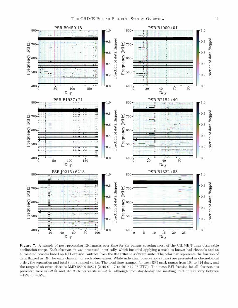
Figure 7. A sample of post-processing RFI masks over time for six pulsars covering most of the CHIME/Pulsar observabledeclination range. Each observation was processed identically, which included applying a mask to known bad channels and anautomated process based on RFI excision routines from the CoastGuard software suite. The color bar represents the fraction ofdata flagged as RFI for each channel, for each observation. While individual observations (days) are presented in chronologicalorder, the separation and total time spanned varies. The total time spanned for each RFI mask ranges from 164 to 324 days, andthe range of observed dates is MJD 58500-58824 (2019-01-17 to 2019-12-07 UTC). The mean RFI fraction for all observationspresented here is ∼20% and the 95th percentile is ∼25%, although from day-to-day the masking fraction can vary between∼15% to ∼68%.

12 CHIME/Pulsar Collaboration et al.

103

S/N Expected

101

102

103

104

105

S/N

Obs

erve

d

20 0 20 40 60 80Declination (deg)

0.1

1

S/N

Rat

io (e

xp/o

bs)

10 3 10 1

Period (s)

10 1

100

101

S/N

Rat

io (e

xp/o

bs)

101 102

DM (pc cm 3)

10 1

100

101

S/N

Rat

io (e

xp/o

bs)

0

1

2

gain

(K/J

y)

400MHz600MHz800MHz

Figure 8. A study of the expected versus observed S/N for 209 pulsars with published flux densities at 600 MHz. Foreach pulsar, the line-of-sight Tsky is estimated from the Haslam sky survey. In each panel, pulsars with declination < 0◦ arehighlighted in blue whereas those with short spin periods of P < 35 ms are highlighted in red. In the top-left panel we showthe expected S/N is shown as a range for each pulsar, where the left edge of each point corresponds to a pessimistic Tsys of100 K and the right edge with a Tsys of 50 K. The diagonal line is the 1:1 ratio, where the observed S/N equals the expectedvalue. The ratio of the expected to observed S/N versus pulsar period (top-middle), and DM (top-right) are also shown. Forsimplicity, the expected S/N for each pulsar is taken to be the averaged value within the range of Tsys. In the lower panel,we show the ratio of the expected to observed S/N versus declination, including the nominal CHIME primary beam responsecorrection. The beam-corrected gain as a function of declination, at 400, 600 and 800 MHz, is also provided.

The CHIME Pulsar Project: System Overview 13

0.5

0.0

0.5

1.0

Nor

mal

ised

inte

nsity

Rawtemplate (I)data (I)template (Q)data (Q)template (U)data (U)template (V)data (V)

0.5

0.0

0.5

1.0

Corrected

100 150 200Phase bin

0.10

0.08

0.06

0.04

0.02

0.00

Diff

eren

ce

100 150 200Phase bin

0.01

0.00

0.01

Figure 9. Comparison of the Stokes profiles from an ob-servation of the main pulse of B1937+21 (solid lines) and atemplate (dashed lines). The top panels shows the uncor-rected data (left) and corrected data (right) for each Stokesparameter: I (black), Q (red), U (magenta) and V (blue).The lower panels shows the residuals between the templateand the raw data (left) and the corrected data (right).

inverse transfer matrix corrections results in a residual

difference of ∼1% or less. For individual pulsars, espe-

cially those which scintillate or exhibit mode changing,

there are instances where the Stokes parameters change

significantly on daily timescales relative to a given tem-

plate.

Ultimately, polarisation stability and calibration is an

on-going challenge for CHIME/Pulsar. Applying the

proposed arbitrary transfer matrix approach to stabilise

the Stokes parameters from day to day will be a nec-

essary step when conducting high-precision timing data

analysis. Further effort will also be made into adapt-

ing this approach to a wideband regime, where the fre-

quency dependence of the polarisation response is also

considered.

4.5. Spectral Leakage

The polyphase filterbank (PFB) used by the CHIME

FX correlator applies a sinc-Hann windowing func-

tion in the Fourier domain to raw digitized sky sig-

nal when forming 1024 frequency channels across the

CHIME band (Bandura et al. 2014). While chosen to

maximize channel sensitivity, the imperfect response in

each synthesized channel produces leakage of signal be-

tween adjacent channels. Coherent dedispersion by the

CHIME/Pulsar backend will ultimately produce alias-

ing of the detected pulsar signal, with a frequency-

dependent lag between the original pulse and its aliased

counterpart across the CHIME band.

0.0 0.2 0.4 0.6 0.8 1.0Pulse Phase

400

450

500

550

600

650

700

750

800

Obs

ervi

ng F

requ

ency

(MH

z)

B1937+21

0.0 0.2 0.4 0.6 0.8 1.0Pulse Phase

J0740+6620

Figure 10. The presence of spectral leakage as dispersedfeatures in CHIME/Pulsar spectra for PSRs J0740+6620 andB1937+21. In both panels, pulse profiles were removed us-ing a principal component analysis for determining de-noisedrepresentations of the on-pulse dynamic spectrum. The spec-trum for B1937+21 was obtained after integrating a single(∼10-min) fold-mode recording, whereas the spectrum forJ0740+6620 was determined by coherently averaging over100 individual epochs of ∼20-min recordings. Vertical arti-facts arise due to imperfect estimation of the de-noised tem-plate profiles.

Figure 10 shows examples of spectral leakage in pulse-

averaged spectra for PSRs B1937+21 and J0740+6620.

Artifacts due to leakage are apparent within a sin-

gle observation of PSR B1937+21 with CHIME/Pulsar,

though similar features are far less prominent in slower,

fainter pulsars like J0740+6620, even after integrating

data taken over 100 epochs as shown in Figure 10.

The MeerTime pulsar-timing backend mitigates spec-

tral leakage in the MeerKAT observing system by us-

ing a modified sinc-Hann windowing function in theirF-engine system; the modified windowing function used

by MeerTime suppresses the response of the synthesized-

channel boundaries, which minimizes leakage but si-

multaneously lowers effective sensitivity in each chan-

nel (Bailes et al. 2016). The commensal nature of pul-

sar/FRB observations with CHIME requires that the F-

engine use the same PFB configuration for all backends

when generating channelized data streams. Therefore,

spectral leakage will be present to varying degrees in

CHIME/Pulsar observations and its impact on timing

will be assessed during offline processing.

4.6. Timing

In order to establish the timing capabilities of the

CHIME/Pulsar system, we collected near-daily ob-

servations of MSPs observed by the North Ameri-

can Nanohertz Observatory for Gravitational Waves

14 CHIME/Pulsar Collaboration et al.

(NANOGrav) during a several-month commissioning pe-

riod when telescope sensitivity was generally stable. We

used timing solutions for online folding that are also

used by NANOGrav at the 305-m Arecibo Observatory

and the 100-m Green Bank Telescope (GBT) for pulsar-

timing data acquisition. Initial “template” pulse profiles

of CHIME/Pulsar data, necessary for cross-correlation

and arrival-time estimation, were generated by excising

channels containing RFI, coherently adding timing data

taken across the commissioning period, and fully aver-

aging the stacked set in time and frequency. The time-

and frequency-averaged profile was then de-noised using

a wavelet transform.

Times of arrival (TOAs) were then computed via

cross-correlation between the template profiles and a

downsampled form of the CHIME/Pulsar fold-mode

timing data. For analysis of NANOGrav pulsars, we

fully integrated available fold-mode data in time and

downsampled in frequency from the native resolution to

32 channels prior to TOA generation, yielding a maxi-

mum of 32 channelized TOAs per epoch. This level of

downsampling is similar to the reduction methods used

by NANOGrav in order to evaluate DM variations over

time (e.g. Levin et al. 2016).

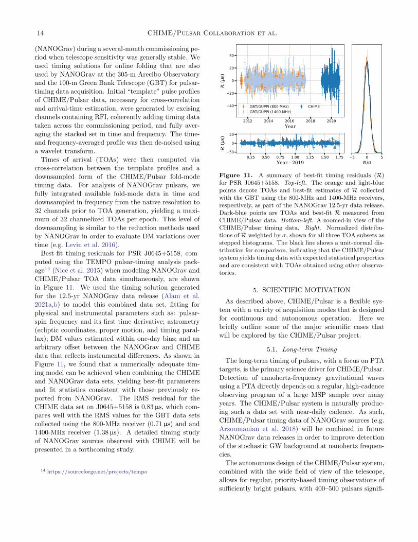
Best-fit timing residuals for PSR J0645+5158, com-

puted using the TEMPO pulsar-timing analysis pack-

age14 (Nice et al. 2015) when modeling NANOGrav and

CHIME/Pulsar TOA data simultaneously, are shown

in Figure 11. We used the timing solution generated

for the 12.5-yr NANOGrav data release (Alam et al.

2021a,b) to model this combined data set, fitting for

physical and instrumental parameters such as: pulsar-

spin frequency and its first time derivative; astrometry

(ecliptic coordinates, proper motion, and timing paral-

lax); DM values estimated within one-day bins; and an

arbitrary offset between the NANOGrav and CHIME

data that reflects instrumental differences. As shown in

Figure 11, we found that a numerically adequate tim-

ing model can be achieved when combining the CHIME

and NANOGrav data sets, yielding best-fit parameters

and fit statistics consistent with those previously re-

ported from NANOGrav. The RMS residual for the

CHIME data set on J0645+5158 is 0.83µs, which com-

pares well with the RMS values for the GBT data sets

collected using the 800-MHz receiver (0.71µs) and and

1400-MHz receiver (1.38µs). A detailed timing study

of NANOGrav sources observed with CHIME will be

presented in a forthcoming study.

14 https://sourceforge.net/projects/tempo

2012 2014 2016 2018 2020Year

40

20

0

20

40

(s)

GBT/GUPPI (800 MHz)GBT/GUPPI (1400 MHz)

CHIME

0.25 0.50 0.75 1.00 1.25 1.50 1.75Year - 2019

50

0

50

(s)

5 0 5/

Figure 11. A summary of best-fit timing residuals (R)for PSR J0645+5158. Top-left. The orange and light-bluepoints denote TOAs and best-fit estimates of R collectedwith the GBT using the 800-MHz and 1400-MHz receivers,respectively, as part of the NANOGrav 12.5-yr data release.Dark-blue points are TOAs and best-fit R measured fromCHIME/Pulsar data. Bottom-left. A zoomed-in view of theCHIME/Pulsar timing data. Right. Normalized distribu-tions of R weighted by σ, shown for all three TOA subsets asstepped histograms. The black line shows a unit-normal dis-tribution for comparison, indicating that the CHIME/Pulsarsystem yields timing data with expected statistical propertiesand are consistent with TOAs obtained using other observa-tories.

5. SCIENTIFIC MOTIVATION

As described above, CHIME/Pulsar is a flexible sys-

tem with a variety of acquisition modes that is designed

for continuous and autonomous operation. Here we

briefly outline some of the major scientific cases that

will be explored by the CHIME/Pulsar project.

5.1. Long-term Timing

The long-term timing of pulsars, with a focus on PTA

targets, is the primary science driver for CHIME/Pulsar.

Detection of nanohertz-frequency gravitational waves

using a PTA directly depends on a regular, high-cadence

observing program of a large MSP sample over many

years. The CHIME/Pulsar system is naturally produc-

ing such a data set with near-daily cadence. As such,

CHIME/Pulsar timing data of NANOGrav sources (e.g.

Arzoumanian et al. 2018) will be combined in future

NANOGrav data releases in order to improve detection

of the stochastic GW background at nanohertz frequen-

cies.

The autonomous design of the CHIME/Pulsar system,

combined with the wide field of view of the telescope,

allows for regular, priority-based timing observations of

sufficiently bright pulsars, with 400–500 pulsars signifi-

The CHIME Pulsar Project: System Overview 15

cantly detected within a single day of operation. This

capability is unprecedented in the northern hemisphere

and only recently achieved for southern pulsars with the

development of the MeerKAT pulsar timing program

(MeerTime; Bailes et al. 2016) and the UTMOST pulsar

instrument (Bailes et al. 2017; Jankowski et al. 2019).

The CHIME/Pulsar system actively monitors observ-

able sources that are reported in the ATNF pulsar cat-

alogue with a range of cadence. CHIME/Pulsar also

observes newly discovered pulsars found by the Green

Bank North Celestial Cap (GBNCC; Stovall et al. 2014)

survey in order to aid in the confirmation and follow-up

of their discovered sources.

5.2. High-cadence Timing of Pulsar-Binary Systems

Long-term timing of binary radio pulsars often yields

secular and/or periodic variations from purely Keplerian

motion. The most famous examples of secular variations

are those associated with general-relativistic orbital de-

cay and precession in compact orbits (see Stairs 2003,

for a review), though many non-relativistic pulsar orbits

have been observed to vary over time due to evolving sky

orientations induced by proper motion (e.g. Kopeikin

1995, 1996). By contrast, the relativistic Shapiro time

delay (Shapiro 1964) is a periodic effect observed in suf-

ficiently inclined binary systems of any size where the

pulsed signal traverses varying amount of spacetime cur-

vature induced the companion star over the course of

the orbit. Measurements of such effects allow for direct

constraints on the masses (e.g., PSR J0740+6622; Cro-

martie et al. 2020) and geometry of the systems in ques-

tion (e.g., PSR J0437−4715; van Straten et al. 2001),

and thus stand to yield high-impact information that is

otherwise inaccessible from purely Keplerian dynamics.

The CHIME/Pulsar system is expected to produce a

rich data set for probing binary astrophysics by monitor-

ing all visible binary pulsars with near-daily observing

cadences over the course of telescope operation. As an

example, Figure 12 shows simulated best-fit estimates

of a timing parameter quantifying relativistic time dila-

tion and gravitational redshift in the PSR J0509+3801

double-neutron-star system (Lynch et al. 2018). While

typical programs observe such sources on monthly or bi-

monthly cadences, the simulated estimates in Figure 12

suggest that such effects can be better constrained with

high-cadence observations – like those achievable with

CHIME/Pulsar – due to quickened evaluations of orbital

parameters and their variations. Moreover, we antici-

pate the daily cadence to yield detections of the Shapiro

delay on timescales much shorter than those typically

seen in current pulsar-timing literature, due to the faster

rate of achieving dense orbital coverage.

0 50 100 150 200 250 300 350Number of Observing Epochs over One Year

6

4

2

0

2

4

6

8

Rel

ativ

istic

Tim

e D

ilatio

n (m

s)

Prediction (DDGR)

Figure 12. Estimates of the relativistic parameter quan-tifying time dilation and gravitational redshift for PSRJ0509+3801 – typically referred to as γ in pulsar-timing lit-erature – derived from simulated TOA data sets with TOAscollected over one year in time but with different observingcadences. For each plotted measurement, a timing data setis generated with tempo assuming that one frequency/time-averaged TOA is obtained per epoch, and that the TOAdata set yields white-noise properties consistent with cur-rent CHIME/Pulsar observations of J0509+3801 (i.e., epoch-averaged RMS residual of ∼70 µs). The red horizontal linemarks the expected value determined by Lynch et al. (2018)when modeling their TOAs using the “DDGR” timing model,that assumes all variations are effects predicted by generalrelativity.

5.3. Plasma propagation effects

Pulsars are sensitive probes of the ISM and its struc-

tural variations across many lines of sight. By process-

ing and recording data at low radio frequencies, the

CHIME/Pulsar system is producing a rich and grow-

ing data set for autonomously monitoring frequency-

dependent features in pulsar data. Examples of such

effects include temporal variation of DM (e.g. Lam et al.

2016; Lentati et al. 2017; Lam et al. 2018), frequency-

dependent DM (Cordes et al. 2016; Donner et al. 2019),

“echoes” in pulsar spectra (e.g. Graham Smith et al.

2011; Michilli et al. 2018; Driessen et al. 2019; Bansal

et al. 2020), “extreme scattering events” in flux density

modulations (e.g. Coles et al. 2015; Kerr et al. 2018),

scintillation (e.g. Bhat et al. 1999b,a,c; Wang et al.

2005, 2008) or multi-path scattering/pulse broadening

(e.g. Bhat et al. 2004; McKee et al. 2018) caused by

small-scale plasma structures. Understanding these ef-

fects is critical in achieving a GW background detection

using PTAs (e.g. Cordes & Shannon 2010; Levin et al.

2016), but are also informative when considering pulsar

16 CHIME/Pulsar Collaboration et al.

astrometry and system dynamics (e.g. Lyne 1984; Pen

et al. 2014; Reardon et al. 2019).

As a demonstration of the suitability of

CHIME/Pulsar for studying small-scale dispersive

variations, we measured the DM time series for

PSR B1937+21, one of the fastest-known MSPs, and

one that is known to exhibit large and rapid variations

in DM (e.g Jones et al. 2017), following the process

detailed in Donner et al. (2019). The 10 highest-S/N

observations were selected, which were phase-aligned

and summed to create a high-S/N frequency-resolved

reference profile, with very little correlated noise. The

original 1024 frequency channels were integrated to

16 channels, and a wavelet smoothing algorithm was

applied, resulting in a noise-free standard template.

The remaining observations in our data set were also

integrated to 16 frequency channels, and TOAs were

measured for each via cross-correlation with the tem-

plate. The TOAs were analysed using TEMPO215

(Hobbs et al. 2006), with a timing model based on the

one presented in Perera et al. (2019), with the time-

varying DM and noise models removed. We fit for DM

on each observing epoch while keeping the other timing-

model parameters fixed to obtain a time series with a

mean cadence of 1.2 days and a median DM precision

of 2.9 × 10−5 pc cm−3, which we present in Figure 13.

As a comparison, the DM time series for B1937+21 ob-

tained from NANOGrav observations with the Arecibo

and Green Bank observatories yield a similar mean DM

precision of ∼2×10−5 pc cm−3, though evaluated over a

monthly cadence Alam et al. (2021a,b). The measured

DM time series from CHIME/Pulsar data displays an

overall linear trend, with additional short-duration ex-

cesses lasting a few tens of days, which would not be

easily-resolved in low-cadence data sets (such as those

normally employed by PTA experiments).

Another important PTA science consideration that

will benefit from the CHIME/Pulsar observing cam-

paign is the study of the Solar wind, which contributes

an annual variation in DM to pulsar timing data. This

effect varies in time, throughout the course of the 11-

yr Solar cycle, and it has been proposed (e.g. Madison

et al. 2019, Tiburzi et al. 2019) that long-term, high-

cadence radio monitoring of pulsars close to the ecliptic

plane will provide valuable information about this phe-

nomenon. Recent work has shown that in high-cadence

data sets with high DM precision, typical simple So-

lar wind models do not adequately-describe the excess

dispersive delay (Tiburzi et al. 2019), and that its ro-

15 https://bitbucket.org/psrsoft/tempo2/src/master

-1

0

1

2

3

4

5

6

58650 58700 58750 58800 58850

ΔD

M (

10

-4 p

c cm

-3)

MJD

Figure 13. DM time series measured from CHIME ob-servations of PSR B1937+21, relative to the initial value of71.01572 pc cm−3. Each observation was integrated in fre-quency to 16 channels, with a TOA measured per chan-nel. The DM was determined by fitting for the frequency-dependent dispersive delay between in-band TOAs for eachday. The median DM uncertainty is 2.9×10−5 pc cm−3. Themean cadence following MJD 58742 is 1.2 days.

bust mitigation will become increasingly important in

searches for low-frequency gravitational waves as pulsar

timing array sensitivity continues to improve (Madison

et al. 2019).

5.4. Polarization

Polarization properties of radio pulsars have pro-

vided a wealth of information about their emission

mechanism and geometry, and about the magnetised

Galactic medium (e.g. Lorimer & Kramer 2004). The

CHIME/Pulsar backend records and stores full Stokes

information, allowing polarization studies to be per-

formed for all detected sources. However, polarization

calibration, necessary for many pulsar studies, is diffi-

cult to obtain for a transit telescope such as CHIME,

where the interplay between the two orthogonal sets

of feeds changes during the observation and is strongly

frequency dependent. Obtaining a beam model of the

telescope accurate enough to recover the intrinsic po-

larization of the signal is a work in progress involving

measurements from various CHIME backends, includ-

ing CHIME/Pulsar (see also Section 4.4). Nevertheless,

even before being able to calibrate the instrument, some

interesting properties of polarized sources can be mea-

sured, and in particular the effect of Faraday rotation.

CHIME/Pulsar, operating at low frequencies and with a

large fractional bandwidth, is able to provide very pre-

cise measurements of rotation measure (RM).

The capability of CHIME/Pulsar to measure precise

RM values has already been demonstrated in a recent

The CHIME Pulsar Project: System Overview 17

work by Ng et al. (2020a), where we present RM values

for 80 pulsars, 55 of which are measured for the first

time. We plan to measure the RM of most detectable

northern pulsars, many of which either do not have a re-

ported RM value, or the catalogued value was measured

decades ago. By virtue of observing a large fraction

of northern pulsars regularly, CHIME/Pulsar will also

significantly contribute to efforts to map the Galactic

magnetic field, complementing similar ongoing studies

at low frequencies (e.g. Lenc et al. 2018; Sobey et al.

2019). In addition, frequent observations present an

exciting opportunity to investigate temporal RM vari-

ations of every observed source. Measuring simultane-

ous DM variations, as described in §5.3, will enable the

measurement of Galactic magnetic field gradient.

5.5. Glitch monitoring

Approximately 200 pulsars to date16 have been ob-

served to exhibit “glitches”, where their rotation pe-

riod abruptly changes and can remain altered for sev-

eral weeks or months subsequently (e.g. Radhakrish-

nan & Manchester 1969; Weltevrede et al. 2011; Mc-

Kee et al. 2016; Lower et al. 2020). Studying glitches

and their aftermath provides insight into the interior

structure of neutron stars and the nuclear equation of

state (e.g. Haskell & Melatos 2015; Haskell & Sedrakian

2018). The modular design the CHIME/Pulsar system

lends itself to immediate, offline analysis of timing vari-

ations consistent with pulsar glitches from many differ-

ent sources, and potentially enables near-realtime alert-

ing of such events to the transient-astronomical commu-

nity. Such analyses are especially interesting in the era

of LIGO/VIRGO detection of GWs, where correlations

of glitch and GW transient events are expected to yield

multi-messenger constraints on the interior structure of

neutron stars. Furthermore, the observing cadence of

the pulsar with a detected glitch can be increased in or-

der to better model the post-glitch recovery properties

of the pulsar.

5.6. Monitoring for emission variability in pulsating

sources

Daily observations, flexible recording configurations,

and a wide observing band are ideal for long-term mon-

itoring of the emission from objects such as repeating

FRBs (e.g. Spitler et al. 2016; CHIME/FRB Collab-

oration et al. 2019a,b; Fonseca et al. 2020), RRATs

(McLaughlin et al. 2006), intermittent (Kramer et al.

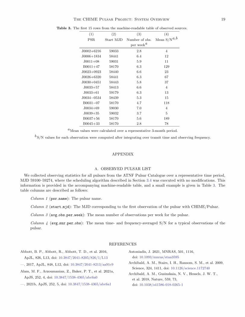
16 See http://www.jb.man.ac.uk/pulsar/glitches/gTable.html andhttp://www.atnf.csiro.au/research/pulsar/psrcat/glitchTbl.html for a list of glitches and their corresponding publications.

2006), nulling (Backer 1970a), and mode-changing pul-

sars (Backer 1970b; Lyne 1971; Naidu et al. 2017). This

will allow us to probe any short and long-term varia-

tion in the rotational properties of the sources and their

potential link with the variability in emission properties

(e.g. Lyne et al. 2010; Perera et al. 2016; Stairs et al.

2019; Naidu et al. 2018).

The high-cadence observations also allow us to search

for previously unknown emission variability in known

pulsars. As a testament to this, Ng et al. (2020b) iden-

tified new nulling and mode changing pulsars from the

commissioning data set (July 2018 to March 2019).

5.7. Searching for pulsars, RRATs, pulses from

repeating FRBs and transient astronomical events

The filterbank mode of the CHIME/Pulsar backend

is being actively used to follow up both unknown sin-

gle pulses of Galactic origin (Good et al., submitted)

and repeating FRB sources discovered by CHIME/FRB.

The large instantaneous field of view and the transit

nature of CHIME/FRB has allowed for the blind de-

tection of these sources. A number of these sources are

then followed up with the more sensitive CHIME/Pulsar

backend as the data are coherently dedispersed to the

DM of the sources, allowing detection of faint pulses

that will otherwise be missed by CHIME/FRB. More-

over, the tracking beams generated for CHIME/Pulsar

remain centered on the positions of the sources during

their transit at the CHIME site, allowing for robust

detection of the intrinsic dynamic spectrum. Further-

more, CHIME/Pulsar has a time resolution of 327.68µs,

three times higher than CHIME/FRB, that could re-

solve smaller scale structures of the single pulses other-

wise undetectable by CHIME/FRB.

Follow-up tracking observations of the unknown

Galactic sources with CHIME/Pulsar is also used to

look for periodicity akin to pulsars and RRATs. These

are done by either measuring the gaps between succes-

sive pulses, or periodicity searches including both Fast

Fourier Transform and “fast folding algorithms” (e.g.

Parent et al. 2018). The new candidates detected by the

CHIME/FRB system and confirmed by CHIME/Pulsar

are subsequently monitored for long-term timing17. New

Galactic discoveries from the use of both CHIME/FRB

and CHIME/Pulsar is reported in Good et al. (2020).

While individual observations of a source with

CHIME/Pulsar are limited by the primary beam size

of CHIME which restricts transit time, the capability to

perform multiple simultaneous observations means that

17 See https://www.chime-frb.ca/galactic

18 CHIME/Pulsar Collaboration et al.

we can afford to repeatedly observe a number of sources

daily to stack and search the data for pulsations. This

will allow for the potential detection of faint sources by

leveraging long integration times. Such strategy has

been employed before in targeted searches of globular

clusters (e.g. Cadelano et al. 2018).

CHIME/Pulsar is also able to rapidly follow up on

any transient astronomical events that might emit radio

pulses. The regular schedule can be overwritten quickly

to point a pulsar beam towards the source of interest

during the forthcoming transit. We expect to apply

the capability to follow up on events such as magne-

tars undergoing X-ray outburst (e.g. Camilo et al. 2006;

Rea et al. 2013; Esposito et al. 2020), gravitational wave

events (Abbott et al. 2016, 2017) and new transitional

MSPs (Archibald et al. 2009).

As with fold-mode observations, filterbank scans of

known or candidate sources are assigned priorities and

included in the automatic scheduling of acquisition with

CHIME/Pulsar. However, it is possible to instead pro-

gram CHIME/Pulsar to operate as a dedicated blind-

search machine. In this case, the FX correlator and

CHIME/Pulsar backend can beamform and process, re-

spectively, up to ∼3000 distinct lines of sight per day

for 5-minute acquisition times.

6. CONCLUSIONS & FUTURE DIRECTIONS

In this work, we reported on a system built for the

CHIME telescope to enable radio pulsar observations in

different modes of acquisition. We described the hard-

ware setup of the CHIME/Pulsar backend and provided

details on the software/networking modules that were

developed to interact with the CHIME FX-correlator

for generating 10 synthesized tracking beams based

on autonomous source selection and scheduling. The

CHIME/Pulsar system operates in tandem with the cos-

mology and FRB experiments, and is capable of regu-

larly recording data in both “fold” and filterbank modes

of pulsar observations. The CHIME/Pulsar system is

poised to make a wide variety of important science

contributions ranging from detailed studies of known

sources and discoveries of new ones, to investigations

of the ISM, both on its own and in collaboration with

other instruments.

ACKNOWLEDGMENTS

We are grateful to the staff of the Dominion Radio

Astrophysical Observatory, which is operated by the Na-

tional Research Council of Canada. CHIME is funded

by a grant from the Canada Foundation for Innova-

tion (CFI) 2012 Leading Edge Fund (Project 31170)

and by contributions from the provinces of British

Columbia, Quebec and Ontario. The CHIME/FRB

Project, which enabled development in common with

the CHIME/Pulsar instrument, is funded by a grant

from the CFI 2015 Innovation Fund (Project 33213) and

by contributions from the provinces of British Columbia

and Quebec, and by the Dunlap Institute for Astronomy

and Astrophysics at the University of Toronto. Addi-

tional support was provided by the Canadian Institute

for Advanced Research (CIFAR), McGill University and

the McGill Space Institute thanks to the Trottier Fam-

ily Foundation, and the University of British Columbia.

The CHIME/Pulsar instrument hardware was funded by

NSERC RTI-1 grant EQPEQ 458893-2014. We thank

Erik C. Madsen for his work in planning the develop-

ment of the CHIME/Pulsar backend. We also thank the

anonymous referee for their feedback and suggestions,

which improved the quality of this work. Pulsar re-

search at UBC is funded by a NSERC Discovery Grant

and by CIFAR. This research was enabled in part by

support provided by WestGrid (www.westgrid.ca) and

Compute Canada (www.computecanada.ca). V.M.K.

holds the Lorne Trottier Chair in Astrophysics & Cos-

mology and a Distinguished James McGill Professor-

ship and receives support from an NSERC Discovery

Grant and Herzberg Award, from an R. Howard Web-

ster Foundation Fellowship from the CIFAR, and from

the FRQNT Centre de Recherche en Astrophysique du

Quebec. D.M. is a Banting Fellow. S.M.R. is a CIFAR

Fellow and is supported by the National Science Foun-

dation (NSF) Physics Frontiers Center award 1430284.

The National Radio Astronomy Observatory is a facility

of the NSF operated under cooperative agreement by

Associated Universities, Inc. P.S. is a Dunlap Fellow

and an NSERC Postdoctoral Fellow. The Dunlap In-

stitute is funded through an endowment established by

the David Dunlap family and the University of Toronto.

C.L. was supported by the U.S. Department of Defense

(DoD) through the National Defense Science & Engi-

neering Graduate Fellowship (NDSEG) Program. M.D.

receives support from a Killam fellowship, NSERC Dis-

covery Grant, CIFAR, and from the FRQNT Centre de

Recherche en Astrophysique du Quebec.

Software: DSPSR (van Straten & Bailes 2011), PSR-

DADA (http://psrdada.sourceforge.net), PSRCHIVE

(Hotan et al. 2004; van Straten et al. 2012), PRESTO

(Ransom 2011), TEMPO (Nice et al. 2015), TEMPO2

(Hobbs et al. 2006)

The CHIME Pulsar Project: System Overview 19

Table 3. The first 15 rows from the machine-readable table of observed sources.

(1) (2) (3) (4)

PSR Start MJD Number of obs. Mean S/Na,b

per weeka

J0002+6216 59033 2.8 4

J0006+1834 58441 6.4 12

J0011+08 59031 5.9 11

B0011+47 58170 6.3 129

J0023+0923 58440 6.6 23

J0026+6320 58441 6.3 67

J0030+0451 58443 5.8 37

J0033+57 58413 6.6 4

J0033+61 59179 6.3 13

J0034−0534 58439 5.3 15

B0031−07 58170 4.7 118

J0034+69 59030 7.0 4

J0039+35 59032 3.7 5

B0037+56 58170 5.6 189

B0045+33 58170 2.8 78

aMean values were calculated over a representative 3-month period.

bS/N values for each observation were computed after integrating over transit time and observing frequency.

APPENDIX

A. OBSERVED PULSAR LIST

We collected observing statistics for all pulsars from the ATNF Pulsar Catalogue over a representative time period,

MJD 59100–59274, where the scheduling algorithm described in Section 3.4 was executed with no modifications. This

information is provided in the accompanying machine-readable table, and a small example is given in Table 3. The

table columns are described as follows:

Column 1 (psr name): The pulsar name.

Column 2 (start mjd): The MJD corresponding to the first observation of the pulsar with CHIME/Pulsar.

Column 3 (avg obs per week): The mean number of observations per week for the pulsar.

Column 4 (avg snr per obs): The mean time- and frequency-averaged S/N for a typical observations of the

pulsar.

REFERENCES

Abbott, B. P., Abbott, R., Abbott, T. D., et al. 2016,

ApJL, 826, L13, doi: 10.3847/2041-8205/826/1/L13

—. 2017, ApJL, 848, L12, doi: 10.3847/2041-8213/aa91c9

Alam, M. F., Arzoumanian, Z., Baker, P. T., et al. 2021a,

ApJS, 252, 4, doi: 10.3847/1538-4365/abc6a0

—. 2021b, ApJS, 252, 5, doi: 10.3847/1538-4365/abc6a1

Antoniadis, J. 2021, MNRAS, 501, 1116,

doi: 10.1093/mnras/staa3595

Archibald, A. M., Stairs, I. H., Ransom, S. M., et al. 2009,

Science, 324, 1411, doi: 10.1126/science.1172740

Archibald, A. M., Gusinskaia, N. V., Hessels, J. W. T.,

et al. 2018, Nature, 559, 73,

doi: 10.1038/s41586-018-0265-1

20 CHIME/Pulsar Collaboration et al.

Arzoumanian, Z., Brazier, A., Burke-Spolaor, S., et al.

2018, ApJS, 235, 37, doi: 10.3847/1538-4365/aab5b0

Backer, D. C. 1970a, Nature, 228, 42, doi: 10.1038/228042a0

—. 1970b, Nature, 228, 1297, doi: 10.1038/2281297a0

Bailes, M., Barr, E., Bhat, N. D. R., et al. 2016, in 2016mks

conf, 11. https://arxiv.org/abs/1803.07424

Bailes, M., Jameson, A., Flynn, C., et al. 2017, PASA, 34,

e045, doi: 10.1017/pasa.2017.39

Bandura, K., Addison, G. E., Amiri, M., et al. 2014,

Canadian Hydrogen Intensity Mapping Experiment

(CHIME) pathfinder, Vol. 9145, 914522,

doi: 10.1117/12.2054950

Bandura, K., Bender, A. N., Cliche, J. F., et al. 2016,

Journal of Astronomical Instrumentation, 5, 1641005,

doi: 10.1142/S2251171716410051

Bansal, K., Taylor, G. B., Stovall, K., & Dowell, J. 2020,

ApJ, 892, 26, doi: 10.3847/1538-4357/ab76bc

Bassa, C. G., Janssen, G. H., Stappers, B. W., et al. 2016,

MNRAS, 460, 2207, doi: 10.1093/mnras/stw1134

Bhat, N. D. R., Cordes, J. M., Camilo, F., Nice, D. J., &

Lorimer, D. R. 2004, ApJ, 605, 759, doi: 10.1086/382680

Bhat, N. D. R., Gupta, Y., & Rao, A. P. 1999a, ApJ, 514,

249, doi: 10.1086/306919

Bhat, N. D. R., Rao, A. P., & Gupta, Y. 1999b, ApJS, 121,

483, doi: 10.1086/313198

—. 1999c, ApJ, 514, 272, doi: 10.1086/306920

Cadelano, M., Ransom, S. M., Freire, P. C. C., et al. 2018,

ApJ, 855, 125, doi: 10.3847/1538-4357/aaac2a

Camilo, F., Ransom, S. M., Halpern, J. P., et al. 2006,

Nature, 442, 892, doi: 10.1038/nature04986

CHIME/FRB Collaboration, Amiri, M., Bandura, K., et al.

2018, ApJ, 863, 48, doi: 10.3847/1538-4357/aad188

—. 2019a, Nature, 566, 235, doi: 10.1038/s41586-018-0864-x

CHIME/FRB Collaboration, Andersen, B. C., Bandura, K.,

et al. 2019b, ApJL, 885, L24,

doi: 10.3847/2041-8213/ab4a80

Christy, B., Anella, R., Lommen, A., et al. 2014, ApJ, 794,

163, doi: 10.1088/0004-637X/794/2/163

Coles, W. A., Kerr, M., Shannon, R. M., et al. 2015, ApJ,

808, 113, doi: 10.1088/0004-637X/808/2/113

Cordes, J. M., & Shannon, R. M. 2010, to be submitted to

ApJ, arXiv:1010.3785. https://arxiv.org/abs/1010.3785

Cordes, J. M., Shannon, R. M., & Stinebring, D. R. 2016,

ApJ, 817, 16, doi: 10.3847/0004-637X/817/1/16

Cromartie, H. T., Fonseca, E., Ransom, S. M., et al. 2020,

NatAs, 4, 72, doi: 10.1038/s41550-019-0880-2

Demorest, P. B., Pennucci, T., Ransom, S. M., Roberts,

M. S. E., & Hessels, J. W. T. 2010, Nature, 467, 1081,

doi: 10.1038/nature09466

Deng, M., & Campbell-Wilson, D. 2014, in 16th

International Symposium on Antenna Technology and

Applied Electromagnetics (ANTEM) (IEEE), 1–2,

doi: 10.1109/ANTEM.2014.6887670

Denman, N., Renard, A., Vanderlinde, K., et al. 2020, JAI,

9, 2050014, doi: 10.1142/S2251171720500142

Donner, J. Y., Verbiest, J. P. W., Tiburzi, C., et al. 2019,

A&A, 624, A22, doi: 10.1051/0004-6361/201834059

Driessen, L. N., Janssen, G. H., Bassa, C. G., Stappers,

B. W., & Stinebring, D. R. 2019, MNRAS, 483, 1224,

doi: 10.1093/mnras/sty3192

Espinoza, C. M., Lyne, A. G., Stappers, B. W., & Kramer,

M. 2011, MNRAS, 414, 1679,

doi: 10.1111/j.1365-2966.2011.18503.x

Esposito, P., Rea, N., Borghese, A., et al. 2020, ApJL, 896,

L30, doi: 10.3847/2041-8213/ab9742

Fonseca, E., Andersen, B. C., Bhardwaj, M., et al. 2020,

ApJL, 891, L6, doi: 10.3847/2041-8213/ab7208

Foster, G., Karastergiou, A., Paulin, R., et al. 2015,

MNRAS, 453, 1489, doi: 10.1093/mnras/stv1722

Good, D. C., Andersen, B. C., Chawla, P., et al. 2020,

submitted to ApJ, arXiv:2012.02320.

https://arxiv.org/abs/2012.02320

Graham Smith, F., Lyne, A. G., & Jordan, C. 2011,

MNRAS, 410, 499, doi: 10.1111/j.1365-2966.2010.17459.x

Haskell, B., & Melatos, A. 2015, IJMD, 24, 1530008,

doi: 10.1142/S0218271815300086

Haskell, B., & Sedrakian, A. 2018, Astrophysics and Space

Science Library, Vol. 457, Superfluidity and

Superconductivity in Neutron Stars (NewCompStar),

401, doi: 10.1007/978-3-319-97616-7 8

Haslam, C. G. T., Salter, C. J., Stoffel, H., & Wilson,

W. E. 1982, A&AS, 47, 1

Hobbs, G. B., Edwards, R. T., & Manchester, R. N. 2006,

MNRAS, 369, 655, doi: 10.1111/j.1365-2966.2006.10302.x

Hotan, A. W., van Straten, W., & Manchester, R. N. 2004,

PASA, 21, 302, doi: 10.1071/AS04022

Jankowski, F., Bailes, M., van Straten, W., et al. 2019,

MNRAS, 484, 3691, doi: 10.1093/mnras/sty3390

Jones, M. L., McLaughlin, M. A., Lam, M. T., et al. 2017,

ApJ, 841, 125, doi: 10.3847/1538-4357/aa73df

Kaplan, D. L., Kupfer, T., Nice, D. J., et al. 2016, ApJ,

826, 86, doi: 10.3847/0004-637X/826/1/86

Karuppusamy, R., Stappers, B. W., & Lee, K. J. 2012,

A&A, 538, A7, doi: 10.1051/0004-6361/201117667

Kerr, M., Coles, W. A., Ward, C. A., et al. 2018, MNRAS,

474, 4637, doi: 10.1093/mnras/stx3101

Kopeikin, S. M. 1995, ApJL, 439, L5, doi: 10.1086/187731

—. 1996, ApJL, 467, L93, doi: 10.1086/310201

The CHIME Pulsar Project: System Overview 21

Kramer, M., Stairs, I. H., Manchester, R. N., et al. 2006,

Science, 314, 97, doi: 10.1126/science.1132305

Lam, M. T., Cordes, J. M., Chatterjee, S., et al. 2016, ApJ,

821, 66, doi: 10.3847/0004-637X/821/1/66

Lam, M. T., Ellis, J. A., Grillo, G., et al. 2018, ApJ, 861,

132, doi: 10.3847/1538-4357/aac770

Lazarus, P., Karuppusamy, R., Graikou, E., et al. 2016,

MNRAS, 458, 868, doi: 10.1093/mnras/stw189

Lenc, E., Murphy, T., Lynch, C. R., Kaplan, D. L., &

Zhang, S. N. 2018, MNRAS, 478, 2835,

doi: 10.1093/mnras/sty1304

Lentati, L., Kerr, M., Dai, S., et al. 2017, MNRAS, 466,

3706, doi: 10.1093/mnras/stw3359

Levin, L., McLaughlin, M. A., Jones, G., et al. 2016, ApJ,

818, 166, doi: 10.3847/0004-637X/818/2/166

Lorimer, D. R., Bailes, M., McLaughlin, M. A., Narkevic,

D. J., & Crawford, F. 2007, Science, 318, 777,

doi: 10.1126/science.1147532

Lorimer, D. R., & Kramer, M. 2004, Handbook of Pulsar

Astronomy, Vol. 4 (Cambridge university press), 54–84

Lower, M. E., Bailes, M., Shannon, R. M., et al. 2020,

MNRAS, doi: 10.1093/mnras/staa615

Lynch, R. S., Swiggum, J. K., Kondratiev, V. I., et al.

2018, ApJ, 859, 93, doi: 10.3847/1538-4357/aabf8a

Lyne, A., Hobbs, G., Kramer, M., Stairs, I., & Stappers, B.

2010, Science, 329, 408, doi: 10.1126/science.1186683

Lyne, A. G. 1971, MNRAS, 153, 27P,

doi: 10.1093/mnras/153.1.27P

—. 1984, Nature, 310, 300, doi: 10.1038/310300a0

Madison, D. R., Cordes, J. M., Arzoumanian, Z., et al.

2019, ApJ, 872, 150, doi: 10.3847/1538-4357/ab01fd

Manchester, R. N., Hobbs, G. B., Teoh, A., & Hobbs, M.

2005, AJ, 129, 1993, doi: 10.1086/428488

Martinez, J. G., Stovall, K., Freire, P. C. C., et al. 2015,

ApJ, 812, 143, doi: 10.1088/0004-637X/812/2/143

McKee, J. W., Lyne, A. G., Stappers, B. W., Bassa, C. G.,

& Jordan, C. A. 2018, MNRAS, 479, 4216,

doi: 10.1093/mnras/sty1727

McKee, J. W., Janssen, G. H., Stappers, B. W., et al. 2016,

MNRAS, 461, 2809, doi: 10.1093/mnras/stw1442

McLaughlin, M. A., Lyne, A. G., Lorimer, D. R., et al.

2006, Nature, 439, 817, doi: 10.1038/nature04440

Michilli, D., Hessels, J. W. T., Donner, J. Y., et al. 2018,

MNRAS, 476, 2704, doi: 10.1093/mnras/sty368

Naidu, A., Joshi, B. C., Manoharan, P. K., &

Krishnakumar, M. A. 2015, ExA, 39, 319,

doi: 10.1007/s10686-015-9450-5

Naidu, A., Joshi, B. C., Manoharan, P. K., &

KrishnaKumar, M. A. 2017, A&A, 604, A45,

doi: 10.1051/0004-6361/201629937

Naidu, A., Joshi, B. C., Manoharan, P. K., &

Krishnakumar, M. A. 2018, MNRAS, 475, 2375,

doi: 10.1093/mnras/stx3284

Ng, C., & CHIME/Pulsar Collaboration. 2017, in IAUS,

2018IAUS 337, 179–182.

https://arxiv.org/abs/1711.02104

Ng, C., Pandhi, A., Naidu, A., et al. 2020a, MNRAS, 496,

2836, doi: 10.1093/mnras/staa1658

Ng, C., Wu, B., Ma, M., et al. 2020b, ApJ, 903, 81,

doi: 10.3847/1538-4357/abb94f

Nice, D., Demorest, P., Stairs, I., et al. 2015, Tempo:

Pulsar timing data analysis. http://ascl.net/1509.002

Parent, E., Kaspi, V. M., Ransom, S. M., et al. 2018, ApJ,

861, 44, doi: 10.3847/1538-4357/aac5f0

Pen, U. L., Macquart, J. P., Deller, A. T., & Brisken, W.

2014, MNRAS, 440, L36, doi: 10.1093/mnrasl/slu010

Perera, B. B. P., Stappers, B. W., Weltevrede, P., Lyne,

A. G., & Rankin, J. M. 2016, MNRAS, 455, 1071,

doi: 10.1093/mnras/stv2403

Perera, B. B. P., DeCesar, M. E., Demorest, P. B., et al.

2019, MNRAS, 490, 4666, doi: 10.1093/mnras/stz2857

Petroff, E., Hessels, J. W. T., & Lorimer, D. R. 2019,

A&A Rv, 27, 4, doi: 10.1007/s00159-019-0116-6

Price, D. C., Staveley-Smith, L., Bailes, M., et al. 2016,

JAI, 5, 1641007, doi: 10.1142/S2251171716410075

Radhakrishnan, V., & Manchester, R. N. 1969, Nature, 222,

228, doi: 10.1038/222228a0

Ransom, S. 2011, PRESTO: PulsaR Exploration and

Search TOolkit. http://ascl.net/1107.017

Rea, N., Esposito, P., Pons, J. A., et al. 2013, ApJL, 775,

L34, doi: 10.1088/2041-8205/775/2/L34

Reardon, D. J., Coles, W. A., Hobbs, G., et al. 2019,

MNRAS, 485, 4389, doi: 10.1093/mnras/stz643

Shapiro, I. I. 1964, PhRvL, 13, 789,

doi: 10.1103/PhysRevLett.13.789

Sobey, C., Bilous, A. V., Grießmeier, J. M., et al. 2019,

MNRAS, 484, 3646, doi: 10.1093/mnras/stz214

Spitler, L. G., Scholz, P., Hessels, J. W. T., et al. 2016,

Nature, 531, 202, doi: 10.1038/nature17168

Stairs, I. H. 2003, LRR, 6, 5, doi: 10.12942/lrr-2003-5

Stairs, I. H., Lyne, A. G., Kramer, M., et al. 2019,

MNRAS, 485, 3230, doi: 10.1093/mnras/stz647

Stovall, K., Lynch, R. S., Ransom, S. M., et al. 2014, ApJ,

791, 67, doi: 10.1088/0004-637X/791/1/67

Thompson, A. R., Moran, J. M., & Swenson, George W., J.

2001, Interferometry and Synthesis in Radio Astronomy,

2nd Edition (Springer, Cham), 59–88

Thornton, D., Stappers, B., Bailes, M., et al. 2013, Science,

341, 53, doi: 10.1126/science.1236789

22 CHIME/Pulsar Collaboration et al.

Tiburzi, C., Verbiest, J. P. W., Shaifullah, G. M., et al.

2019, MNRAS, 487, 394, doi: 10.1093/mnras/stz1278

van Straten, W. 2006, ApJ, 642, 1004, doi: 10.1086/501001

van Straten, W., & Bailes, M. 2011, PASA, 28, 1,

doi: 10.1071/AS10021

van Straten, W., Bailes, M., Britton, M., et al. 2001,

Nature, 412, 158, doi: 10.1038/35084015

van Straten, W., Demorest, P., & Oslowski, S. 2012,

AR&T, 9, 237. https://arxiv.org/abs/1205.6276

Verbiest, J. P. W., Lentati, L., Hobbs, G., et al. 2016,

MNRAS, 458, 1267, doi: 10.1093/mnras/stw347

Wang, N., Manchester, R. N., Johnston, S., et al. 2005,

MNRAS, 358, 270, doi: 10.1111/j.1365-2966.2005.08798.x

Wang, N., Yan, Z., Manchester, R. N., & Wang, H. X.

2008, MNRAS, 385, 1393,

doi: 10.1111/j.1365-2966.2008.12864.x

Weltevrede, P., Johnston, S., & Espinoza, C. M. 2011, in

AIPC, Vol. 1357, 109–112, doi: 10.1063/1.3615091

Yu, H.-R., Zhang, T.-J., & Pen, U.-L. 2014, PhRvL, 113,

041303, doi: 10.1103/PhysRevLett.113.041303