Discussion Paper Deutsche Bundesbank No 07/2013 China‘s role in global inflation dynamics Sandra Eickmeier Markus Kühnlenz Discussion Papers represent the authors‘ personal opinions and do not necessarily reflect the views of the Deutsche Bundesbank or its staff.
Transcript
Discussion PaperDeutsche BundesbankNo 07/2013
China‘s role in global inflation dynamics
Sandra EickmeierMarkus Kühnlenz
Discussion Papers represent the authors‘ personal opinions and do notnecessarily reflect the views of the Deutsche Bundesbank or its staff.
Editorial Board: Klaus Düllmann Heinz Herrmann Christoph Memmel
Deutsche Bundesbank, Wilhelm-Epstein-Straße 14, 60431 Frankfurt am Main, Postfach 10 06 02, 60006 Frankfurt am Main Tel +49 69 9566-0 Please address all orders in writing to: Deutsche Bundesbank, Press and Public Relations Division, at the above address or via fax +49 69 9566-3077
Internet http://www.bundesbank.de
Reproduction permitted only if source is stated.
ISBN 978–3–86558–8ISBN 978–3–86558–8
92–0 (Internetversion) 91–3 (Printversion)
Non-technical summary
The global dimension of inflation has become a popular theme for economic researchersin academia and central banks. It has been shown that inflation rates across countriesstrongly comove due to domestic inflation rates being determined, among others, by for-eign or global common forces. China’s role in these developments is, however, still some-what unclear.The significance of China for the world economy has risen enormously over the past 20
years in terms of both GDP and trade. Observers have speculated whether (positive) de-mand effects in China and subsequent positive effects on international price developments(via rising export and commodity prices) or whether supply effects and subsequent pricedampening effects (via declining import prices and competitive pressures) have dominatedin the past and, hence, what the net effect of these developments was. The goal of thisanalysis is to examine empirically the role of Chinese supply and demand shocks in globalinflation dynamics and to shed light on the transmission mechanism.We apply a structural dynamic factor model to a large quarterly dataset of 38 coun-
tries (including China) between 2002 and 2011 to analyze China’s role in global inflationdynamics. We identify Chinese supply and demand shocks and examine their contribu-tions to global price dynamics and the transmission mechanism. Our main findings areas follows. (i) Chinese supply and demand shocks affect prices in other countries signifi-cantly. Demand shocks matter slightly more over the sample period than supply shocks.Producer prices tend to be more strongly affected than consumer prices by Chinese shocks.The overall share explained of international inflation by Chinese shocks is notable (about5 percent on average over all countries but not more than 13 percent in each region). (ii)Both direct channels (via import and export prices) and indirect channels (via greaterexposure to foreign competition and commodity prices) seem to matter. (iii) Differencesin trade exposure (overall and with China) as well as commodity exposure help explainingcross-country differences in price responses.
Nicht-technische Zusammenfassung
Der globale Zusammenhang zwischen Inflationsraten ist zu einem beliebten Thema fürWirtschaftsforscher in Universitäten und Zentralbanken geworden. So ist etwa gezeigtworden, dass Inflationsraten über Ländergrenzen hinweg einen Gleichlauf aufweisen, weildie heimische Teuerung unter anderem von gemeinsamen ausländischen beziehungsweiseglobalen Kräften getrieben wird. Die Rolle Chinas innerhalb dieses Wirkungsgeflechts istjedoch noch weithin ungeklärt.Die Bedeutung Chinas für die Weltwirtschaft, gemessen an seinem Anteil sowohl am
Bruttoinlandsprodukt als auch am internationalen Handel, ist in den letzten 20 Jahrenenorm gestiegen. Beobachter spekulieren darüber, ob in der Vergangenheit (positive)Nachfrageeffekte aus China mit preissteigernder Wirkung (etwa über höhere Export- undRohstoffpreise) dominierten oder aber Angebotseffekte mit preisdämpfendem Effekt (überniedrigere Importpreise und verstärkten Wettbewerbsdruck) und mithin, wie groß derEinfluss Chinas per saldo gewesen ist.Wir wenden ein strukturelles dynamisches Faktormodell auf einen umfangreichen Satz
vierteljährlicher Daten für 38 Länder (einschließlich Chinas) über dem Zeitraum von 2002bis 2011 an, um die Rolle Chinas in der globalen Inflationsentwicklung zu untersuchen.Wir identifizieren chinesische Angebots- und Nachfrageschocks, schätzen deren Beiträgezur globalen Preisentwicklung ab und beleuchten den Transmissionsmechanismus. Unserewichtigsten Ergebnisse sind wie folgt. (i) Chinesische Angebots- und Nachfrageschocksüben einen signifikanten Einfluss auf Preise in anderen Ländern aus. Dabei sind Nach-frageschocks im Beobachtungszeitraum etwas bedeutsamer gewesen als Angebotsschocks.Der gesamte Anteil an der globalen Inflation, den chinesische Schocks erklären, ist nichtzu vernachlässigen (rund 5 Prozent im Durchschnitt aller Länder, aber nicht mehr als 13Prozent in einzelnen Regionen). (ii) Sowohl direkte Wirkungskanäle (über Import- undExportpreise) als auch indirekte (über internationalen Wettbewerbsdruck und Rohstoff-preise) sind von Bedeutung. (iii) Unterschiede zwischen einzelnen Ländern in der Preis-reaktion können auf den Grad der internationalen Handelsverflechtung (insgesamt undmit China) und auf die Bedeutung von Rohstoffen für die Volkswirtschaften zurückge-führt werden.
China’s Role in Global Inflation Dynamics∗
Sandra Eickmeier† Markus Kühnlenz‡
Abstract
We apply a structural dynamic factor model to a large quarterly dataset covering
38 countries between 2002 and 2011 to analyze China’s role in global inflation dynam-
ics. We identify Chinese supply and demand shocks and examine their contributions
to global price dynamics and the transmission mechanism. Our main findings are:
(i) Chinese supply and demand shocks affect prices in other countries significantly.
Demand shocks matter slightly more than supply shocks. Producer prices tend to be
more strongly affected than consumer prices by Chinese shocks. The overall share
of international inflation explained by Chinese shocks is notable (about 5 percent on
average over all countries but not more than 13 percent in each region); (ii) Direct
channels (via import and export prices) and indirect channels (via greater exposure
to foreign competition and commodity prices) seem both to matter; (iii) Differences
in trade (overall and with China) and in commodity exposure help explaining cross-
country differences in price responses.
JEL classification: F41, E31, C3
Keywords: Global inflation, China, international business cycles, structural dynamic
factor model, sign restrictions
∗We wish to thank Knut Are Aastveit, Heinz Herrmann, Ulf Slopek and Mu-Chun Wang as well asthe participants of a joint Norges Bank-Bundesbank workshop, of the 4th workshop on Money, Macro andFinance in East Asia and of a seminar at the Reserve Bank of Australia for very helpful comments anddiscussions. The opinions expressed in this paper are those of the authors and do not necessarily reflectthe views of the Deutsche Bundesbank.
The global dimension of inflation has become a popular theme for economic researchers
in academia and at central banks. As shown, for example, by Ciccarelli and Mojon (2010)
and Mumtaz and Surico (forthcoming), inflation rates across countries strongly comove
due to domestic inflation rates being determined, among other things, by external or global
forces (e.g. Borio and Filardo (2007), Eickmeier and Pijnenburg (2013)).
At the same time, China’s significance for the world economy has increased enormously
over the past 20 years in terms of GDP and trade.1 China’s growth has been driven by
fundamental changes on both the supply side and the demand side. Labor has been amply
supplied at low wages, and in labor-intensive segments, China has achieved a leading
market position. Moreover, privatization and trade liberalization have triggered a shift of
resources across and within sectors leading to a surge in manufacturing productivity (Zhu
(2012)).2 In addition, China has greatly diversified its export goods and improved the
quality of its products. While churning out manufactured goods for consumers worldwide,
China has become a major, and often dominant importer of commodities. With incomes
on the rise, China’s internal demand and appetite for both capital and consumer goods
produced abroad has expanded rapidly as well.
It is likely that these developments have affected other countries’ (subsequently la-
beled "foreign" as opposed to Chinese) inflation rates and contributed to their comove-
ment. Most observers have focused on positive demand effects from China on foreign
prices through rising export and commodity prices and on price-dampening supply effects
through low-cost production in China and subsequently declining import prices as well as
lower profit margins as a consequence of competitive pressures. It has also been suggested
that the mix of influences might have changed recently with wages in China on the rise
(Li, Li, Wu and Xiong (2012)).
Whether positive macroeconomic developments in China are quantitatively important
for foreign inflation rates, whether they have affected foreign prices positively or negatively
and through which channels is far from clear.
The goal of this analysis is to examine empirically the role of Chinese supply and
demand shocks in global inflation dynamics and to shed light on the transmission mech-
anism. For that purpose, we use a structural dynamic factor model (DFM) which has
1China is now the second-largest economy and achieved a 10 percent share of global output in 2011, asmeasured by current prices and market exchange rates. China’s nominal exports have grown at an averageannual rate of 22 percent since its accession to the World Trade Organization (WTO) in December 2001,compared with an 11 percent annual expansion of world trade over the same period. As a result, China’sshare of (nominal) world exports is now almost 11 percent, making it the largest trading nation. Around12 percent of OECD countries’ total imports came from China; in manufactured goods alone, the share isat 19 percent.
2A formal growth model based on reallocation between low-productivity state-owned firms and high-productivity private enterprises within the manufacturing sector has been proposed by Song, Storeslettenand Zilibotti (2011).
�
been suggested by Forni, Hallin, Lippi and Reichlin (2000). The DFM allows rich and
flexible modelling of the different ways in which shocks propagate throughout the world,
while keeping dimensionality manageable. We estimate factors from two separate large
datasets, one set of Chinese and one set of foreign quarterly macroeconomic variables
from 2002 to 2011. The latter dataset contains more than 800 quarterly macroeconomic
variables from 37 advanced and emerging market economies, covering, for each country,
several price measures (including consumer and producer prices, exchange rates, commod-
ity prices, labor costs) and other variables which are useful in analyzing the transmission
channels (including interest rates, monetary aggregates, real activity variables). We model
the Chinese and the global factors together in a vector autoregression (VAR). Chinese
supply and demand shocks are then identified by imposing sign restrictions on short-run
impulse response functions. We provide results on the shocks’ dynamic transmission to
foreign consumer and producer prices. We then analyze the propagation mechanism (i)
by looking at the impulse responses of variables capturing the transmission channels of
Chinese shocks and (ii) by trying to explain cross-country differences in price reactions
with differences in country characteristics such as openness, exposure to commodities, the
degree of regulation on labor and goods markets and the economic structure. We also
carry out variance decompositions of international inflation dynamics in order to assess
the importance of Chinese supply and demand shocks over the sample period.
Our main findings are as follows: (i) Chinese supply and demand shocks significantly
affect prices in other countries. Demand shocks matter slightly more between 2002 and
2011 than supply shocks. Producer prices tend to be more strongly affected than are
consumer prices by Chinese shocks. The overall share of foreign inflation explained by
Chinese shocks is notable (about 5 percent on average over all countries but not more
than 13 percent in each region); (ii) Direct channels (via import and export prices) and
indirect channels (via greater exposure to foreign competition and commodity prices)
both seem to matter; (iii) Differences in trade (overall and with China) and in commodity
exposure help explaining cross-country differences in price responses.
The rest of the paper is structured as follows. In Section 2, we briefly review the
literature that is most relevant to our paper and set out our contributions. We present
the DFM framework in Section 3. In Section 4, we provide details on the data. Section 5
presents impulse response results on the international transmission of Chinese supply and
demand shocks and contributions made by the shocks to inflation in other countries. It
also sheds light on the transmission mechanisms and presents several robustness checks.
Section 6 concludes.
�
2 Related literature and contributions
Our paper is closely related to the recent empirical literature on global inflation, accord-
ing to which inflation rates comove strongly across countries (Ciccarelli and Mojon (2010),
Mumtaz and Surico (forthcoming)). Ciccarelli and Mojon (2010) extract common factors
from a large set of advanced economies’ inflation rates and find that the first factor alone
explains 40-90 percent of inflation and 2-80 percent of detrended inflation, depending on
the country. Mumtaz and Surico (forthcoming) pool various inflation rates for advanced
countries and estimate both country-specific and world factors using a factor model with
time-varying parameters. They find that world factors contribute between virtually noth-
ing and about 10 percent to the variation in inflation rates since 1995.
Other studies analyze the reasons for highly synchronized inflation rates (and output
growth), while focusing on the role of China. Osorio and Unsal (2011) examine the inter-
national transmission of shocks from China to foreign inflation using a Global VAR model
and generalized impulse response functions.3 They look at the transmission of Chinese
output shocks to world commodity prices and to Australasian economies. They find that
such shocks, which also raise consumer price inflation and output in China (and hence,
can be regarded as Chinese demand shocks), cause world commodity prices to increase
temporarily after a delay of two quarters. Direct effects in the transmission to other
countries’ prices (through higher imported goods prices) are found to be more important
than indirect effects (through an increase in commodity prices). Aggregate (domestic and
foreign) demand and supply shocks appear to contribute about 60 percent and 40 percent,
respectively, to China’s inflation. Furthermore, more than 80 percent of China’s inflation
is explained by domestic shocks, about 2 percent by regional shocks, and the rest by global
shocks. Regional shocks (which now include Chinese shocks) do not explain more than 10
percent in any Asian country under investigation and a very small percentage also in New
Zealand, but they account for roughly one-fifth of the fluctuations in Australia’s prices.
Côté and de Resende (2008) is another very closely related study. It assesses China’s
role for inflation in 18 OECD countries between 1984 and 2006 by estimating dynamic
inflation equations and by analyzing the various transmission channels listed in the intro-
duction by means of counterfactual experiments. The authors find that the overall effect of
economic fluctuations in China on inflation in most countries is negative, suggesting that
supply effects from expansionary shocks dominate demand effects. The most important
transmission channel appears to be competition with domestic suppliers. Moreover, the
role of China is found to have increased over time.
Finally, there are studies which focus on one or few individual channels of transmission
3Cesa-Bianchi, Pesaran, Rebucci and Xu (forthcoming) and Feldkircher and Korhonen (2012) use GlobalVARs to assess the transmission of Chinese output shocks to output in other regions also using generalizedimpulse response functions. They do not look at inflation reactions.
�
of Chinese shocks to other countries’ inflation. Mandel (2013) assesses the relationship
between Chinese competition and two components of US import prices: marginal costs
and markups. He finds evidence for non-Chinese exporters having experienced a squeeze
in markups and having shifted towards higher quality products which resulted in increased
marginal costs as a consequence of China entering into exporting. Feyziogulu and Willard
(2006), Kumar, Taimur, Decressin, MacDonagh and Feyziogulu (2003), Kamin, Marazzi
and Schindler (2006) and Morel (2007) analyze the role of import prices and find a mod-
erate decline in inflation rates in advanced economies and Asia through that channel.
Roache (2012) finds a limited role of shocks to Chinese activity for world commodity
prices. Aastveit, Bjoernland and Thorsrud (2012) look at the contribution of emerging
compared with advanced economies’ demand to oil price fluctuations and find the former
(particularly demand from emerging Asia) to be more important than the latter.
We make several contributions to the literature. First, and most importantly, our
model allows us to include a large number of variables from many countries and, hence,
to analyze not only the net effect on inflation of Chinese macroeconomic developments,
but also to investigate the transmission mechanism in greater detail than previous studies
do. We look at direct channels (via trade) and indirect channels (via commodity prices
and greater exposure to foreign competition). Second, we focus on identified, orthogonal
shocks, unlike the Global VAR studies presented above which use generalized impulse
responses to non-orthogonal shocks which are hard to interpret economically. Third,
compared to other studies estimating the impact of foreign influences on domestic inflation
based, for example, on Phillips curves (Borio and Filardo (2007), Eickmeier and Pijnenburg
(2013)) we fully account for interaction between foreign variables and between foreign and
Chinese variables.
3 The structural dynamic factor model
The analysis departs from two NCN - and NG-dimensional vectors XCNt and XG
t . XCNt
includes a large number (NCN ) of economic variables for China, and XGt , the "global data-
set", includes a large number (NG) of series from other countries. Let Xt = (XCN ′t , XG′
t )′
and N = NCN +NG. Xt is modeled using an approximate dynamic factor model (Bai and
Ng (2002), Stock and Watson (2002b)):
Xt = Λ′Ft + et (3.1)
In equation (3.1), Ft = (f1t, . . . , frt)′ and et = (e1t, . . . , eNt)
′ denote, respectively, a
vector of common factors that have a major effect on all foreign and Chinese variables
and may thus be regarded as the main (common) drivers of the foreign economies, and a
vector of variable-specific (or idiosyncratic) components. The number of common factors
�
is generally much smaller than the number of variables contained in the dataset, i.e.
r << N . In addition, Ft may contain dynamic factors and their lags. To that extent,
equation (3.1) is not restrictive. Common and variable-specific components are orthogonal.
The common factors are also assumed to be orthogonal to each other, and the variable-
specific components can be weakly correlated with one another and also serially correlated
in the sense of Chamberlain and Rothschild (1983). The matrix of factor loadings is
Λ = (λ1, . . . , λN ), where λi is an r-dimensional vector whose elements measure the effect
of each factor on variable i, i = 1, ..., N .
It is assumed that the dynamics of the factors can be described using a VAR(p) model:
Since factors are estimated from demeaned data, there is no need to consider constants in
the VAR.
We break down the r-dimensional vector of factors Ft into an rCN -dimensional vector
of unobserved (or latent) Chinese factors FCNt and an rG = r − rCN -dimensional vectorof unobserved global factors FGt , i.e. Ft = (FCN ′t , FG′t )′. The vector of innovations wtdepends on Chinese and global shocks.
The model can be estimated in six steps. The first step is to estimate the rCN Chinese
factors from the Chinese dataset with principal components, which yields F̂CNt . Second,
we remove the influence of the Chinese factors from the international data. This is achieved
by regressing each element ofXGt on F̂
CNt . This helps reducing the dimension of the VAR.4
Third, we estimate the global factors from the set of residuals from those regressions, which
yields F̂Gt . Fourth, we estimate the matrix of factor loadings Λ by an OLS regression of
Xt on (F̂CNt ′, F̂Gt ′)′. Fifth, we estimate the VAR (3.2) with OLS equation-wise. Sixth, weidentify Chinese supply and demand shocks, as explained in detail below.
The numbers of common global and Chinese factors are determined throughout the
paper by the information criterion ICp2 of Bai and Ng (2002), which has been shown to
perform well in small samples. According to this criterion, we set rCN and rG to 2. 2
factors explain 39 percent of the variation in the Chinese dataset, and 2 "global" factors
explain 25 percent of the variation in the international data (after having removed the
Chinese influence). We will show in the robustness check section below that increasing
the number of factors does not alter our main results.
To identify the Chinese supply and demand shocks, we first apply a Cholesky decompo-
sition to the covariance matrix of the reduced-form VAR residuals wt. The orthogonalized
shocks vt are related to the reduced-form residuals as follows: vt = Φwt.
We then rotate vt and impose sign restrictions to identify Chinese supply and demand
4We have repeated the entire analysis without this "cleaning step". Cleaning does not have a majoreffect on our main results. Results are available upon request.
�
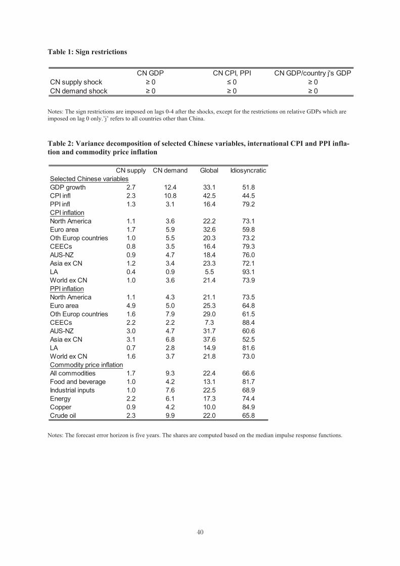
shocks, which are given by two elements of ηt = Rvt. We restrict supply shocks to
move Chinese real activity (measured by GDP) and prices (measured by CPI and PPI)
in opposite directions, whereas demand shocks are assumed to move them in the same
direction. Moreover, the Chinese shocks are restricted to have a stronger impact on
Chinese GDP than on all other countries’ GDP. All other (rG global) shocks are, in
addition, restricted not to have the same characteristics as the Chinese shocks. The sign
restrictions are summarized in Table 1. They are imposed on the contemporaneous impulse
responses and the first four lags except for the sign restrictions on relative GDP which are
imposed on impact only.
The sign restrictions on Chinese activity and prices are consistent with a large number
of theoretical models (e.g. the IS-LM model or new Keynesian models such as Smets and
Wouters (2003)) and have been used before in empirical work (e.g. Peersman (2005)). We
restrict both consumer and producer prices since they are not based on the same basket of
goods (and services). The food component is very important in the Chinese CPI accounting
for roughly 30 percent of China’s CPI basket (ADB (2011)), whereas other goods such
as industrials which have a large weight in trade among advanced economies receive a
greater weight in the PPI. Restrictions on one variable relative to another variable (Chinese
relative to other countries’ GDP in our case) have also been applied in empirical work
before in similar (Farrant and Peersman (2006)) and in other contexts (e.g. Eickmeier and
Ng (2011), Furlanetto, Ravazzolo and Sarferaz (2012)). We also emphasize that it is less
restrictive to apply the sign restrictions on relative GDP rather than, for example, ordering
Chinese factors before global factors or vice versa and applying zero contemporaneous
restrictions. Our identification scheme allows Chinese factors to react immediately to
global shocks and global factors to react immediately to Chinese shocks, which would not
have been the case under either of the two possible alternative orderings.
The identification is implemented using the method by Rubio-Ramírez, Waggoner and
Zha (2010). It is well known that sign restrictions do not allow us to achieve unique
identification of shocks (see Fry and Pagan (2011)). Instead, a large number of models
are consistent with the restrictions. We draw rotation matrices until 200 of them yield
us shocks consistent with the sign restrictions. We adopt the "Median Target" approach
suggested by Fry and Pagan (2007) to pick among all models the one which yields impulse
responses of Chinese GDP and prices to the two shocks close to the median impulse
responses. For more details on the implementation of the sign restrictions, see Rubio-
Ramírez et al. (2010) and Fry and Pagan (2007).
Impulse responses to the Chinese shocks of the individual variables in the large datasets
can be computed as weighted averages over impulse responses of estimated Chinese and
global factors where the weights are the estimated loadings. We show below median
impulse responses and 90% confidence bands which reflect parameter (not model) uncer-
tainty. We assess below how large model uncertainty is and whether not considering it in
�
our baseline poses a problem. The confidence bands are constructed using the bootstrap-
after-bootstrap methodology proposed by Kilian (1997) with 400 replications. In the boot-
strap, we neglect the uncertainty involved with the factor estimation following Bernanke,
Boivin and Eliasz (2005) because of the large cross-section dimensions.5
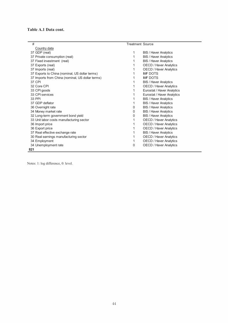
4 Data
Our sample period is 2002Q1-2011Q2 and therefore starts just after China’s accession to
the WTO in December 2001. We test robustness with respect to the sample period, which
we extend back to 1995Q4 in the robustness check section.
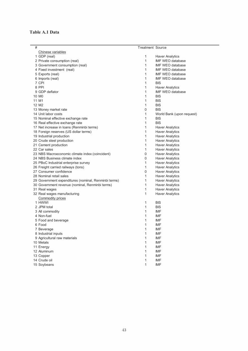
The Chinese dataset contains NCN = 32 macroeconomic variables. It comprises sev-
eral activity indicators, price and cost measures, survey-based confidence and expectation
measures, monetary aggregates and interest rates.
The global dataset includes data for 37 countries, if available: OECD countries, Brazil,
Colombia and several emerging Asian economies (i.e. Thailand, Indonesia, Malaysia, Tai-
wan and Singapore). Including the last-named group of countries helps us to disentangle
Chinese shocks from shocks stemming from the rest of Emerging Asia. The variables con-
ernment bond yields), a broad monetary aggregate M2, real economic activity indicators
(GDP, personal consumption, fixed investment, employment, the unemployment rate, ex-
ports (total and to China), imports (total and from China), price and cost variables (CPI,
PPI, GDP deflator, earnings6, unit labor costs7, import and export prices, exchange rates).
In addition, several international commodity price aggregates and selected price series for
single commodities are included. The overall number of series contained in the global
dataset is NG = 821.
For the international dataset, we largely rely on series provided by the OECD’s Main
Economic Indicators (MEI) database and the IMF’s World Economic Outlook (WEO)
database. For China, we mainly use official national data as provided by Haver Analytics.
Some series were available only at annual frequency, especially a few series from China,
and we interpolated them using the cubic spline method. Since the factor model requires
the variables to be stationary, they were transformed accordingly. We include interest rates
and unemployment rates in levels and all other variables in quarter-on-quarter differences
of the logarithms. Outliers were removed following the procedure proposed by Stock and
5Boivin and Ng (2006) show in Monte Carlo simulations that about 30 series are sufficient to obtainaccurate factor forecasts using principal components.
6According to the OECD definition, earnings include overtime payments and various bonuses in additionto basic wages, whereas employer contributions to social security (which would be included in compensationof employees) are not taken into account.
7We use, when available, a smoothed series of the unit labor costs in the manufacturing sector providedby national sources. The smoothed series are published by the OECD.
�
Watson (2005).8 Our dataset is unbalanced, i.e. some series are not available over the
entire sample period. We use the expectation maximization (EM) algorithm to interpolate
these series (see Stock and Watson (2002a) for details). We only interpolate (and include)
data for which at least five years of data are available. Finally, we normalize each series
to have a zero mean and a unit variance.
An overview of the complete datasets is provided in Table A.1.
5 Results
In this section, we first show impulse responses to Chinese supply and demand shocks
and variance decompositions of the (key) Chinese variables which we restricted for shock
identification (GDP and prices). We then analyze the shock transmission to international
prices. We also present variance decompositions for international inflation rates. To limit
the number of results shown we provide impulse responses and variance decompositions
for consumer and producer prices on average over countries belonging to specific regions:
Spain, Finland, France, Greece, Ireland, Italy, Netherlands, Portugal), "Other European
countries" (Switzerland, Denmark, United Kingdom, Norway, Sweden), "CEECs" (Cen-
tral and East European countries: Czech Republic, Estonia, Hungary, Poland, Slovenia,
Slovakia), "Australia-New Zealand", "Asia ex CN" (Japan, Korea, Thailand, Indonesia,
Malaysia, Singapore, Taiwan) and "Latin America" (Chile, Mexico, Brazil, Colombia).
Results are aggregated using nominal GDP weights (in US dollar terms based on market
exchange rates) averaged over our sample period. To analyze the transmission mecha-
nism, we then provide impulse responses of variables capturing the different transmission
channels and relate individual countries’ reactions to the shocks to country-specific char-
acteristics. Finally, we carry out robustness checks.
5.1 Chinese supply and demand shocks and transmission to key Chinese
variables
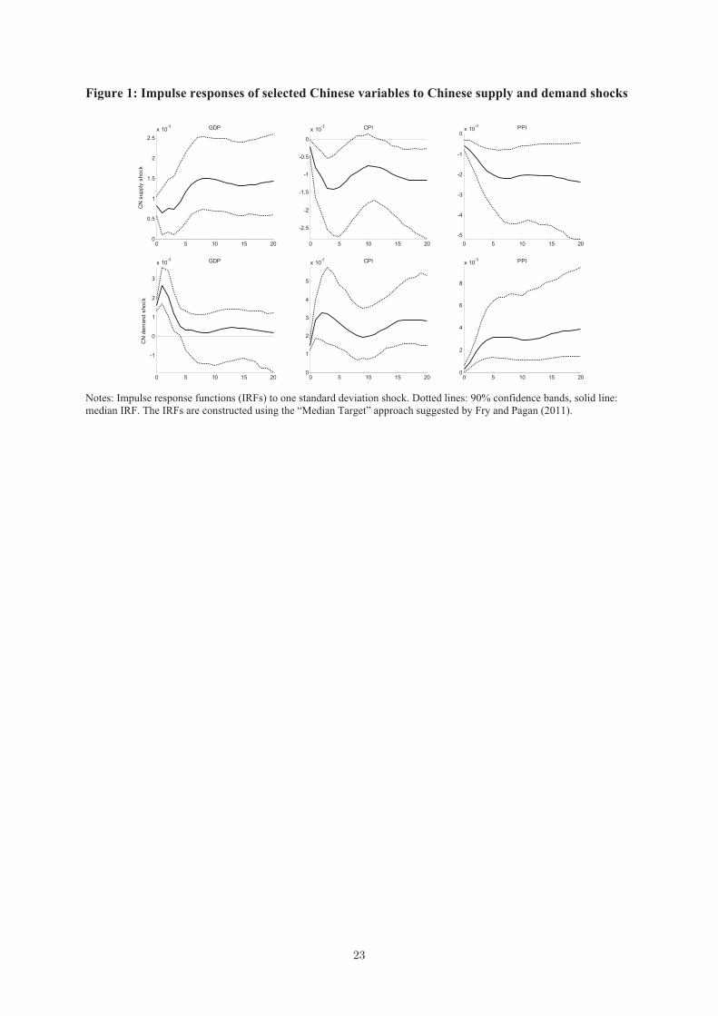
Figure 1 shows reactions of key Chinese variables to the Chinese supply and demand
shocks. The Chinese supply shock has a permanent positive effect on GDP, which rises on
impact by almost 0.1 percent (median response) and then increases further to more than
0.15 percent after seven quarters. The effects of the supply shock on Chinese CPI and PPI
are very long-lasting (they decline by about 0.1 percent and 0.2 percent, respectively). The
Chinese demand shock has an immediate, but temporary positive effect on Chinese GDP.
The maximum of more than 0.2 percent is achieved after one quarter. Chinese consumer
8Outliers are here defined as observations of the stationary data with absolute median deviations largerthan three times the interquartile range. They are replaced by the median value of the preceding fiveobservations.
and producer prices rise permanently by about 0.3 percent. Overall, the shapes of the
impulse responses are broadly as expected.
We also looked at responses of other Chinese variables, which our structural dynamic
factor model allows us to do (we do not show them so as not to overload the paper) and
which helps us to better understand the characteristics of the identified aggregate supply
and demand shocks. We note that the aggregate supply and demand shocks summarize,
for example, markup, labor supply and technology shocks and preference and investment
shocks, respectively. One notable feature of the (positive) Chinese supply shock is that it
leads to an increase in real wages in China which are probably driven by the technology
shock component rather than by the markup or labor supply shock components. Those
latter shocks would imply a decline in real wages. We will discuss below how this may
affect the interpretation of our results for other countries.
Table 2 shows forecast error variance shares of the Chinese variables explained by
Chinese supply and demand shocks (first two columns), other global shocks (third column)
and idiosyncratic components (last column). The shares were computed from the median
impulse responses at the five-year horizon. Chinese supply and demand shocks have some
explanatory power for Chinese GDP growth (3 and 12 percent, respectively) and inflation
(between 1 and 11 percent, respectively). Global shocks account for 33 percent of Chinese
GDP growth and for 16-43 percent of inflation. The finding that demand shocks are more
important for inflation in China than supply shocks and the percentage share explained
by global shocks of Chinese inflation are broadly in line with Osorio and Unsal (2011).
Idiosyncratic components seem to matter quite a lot for Chinese variables which might
be due (partly) to the poor quality of Chinese data. We will discuss whether or not this
poses a problem in our setup in the robustness section below.
5.2 Transmission of Chinese supply and demand shocks to international
prices
Figures 2 and 3 show the effects of the Chinese shocks on foreign consumer and producer
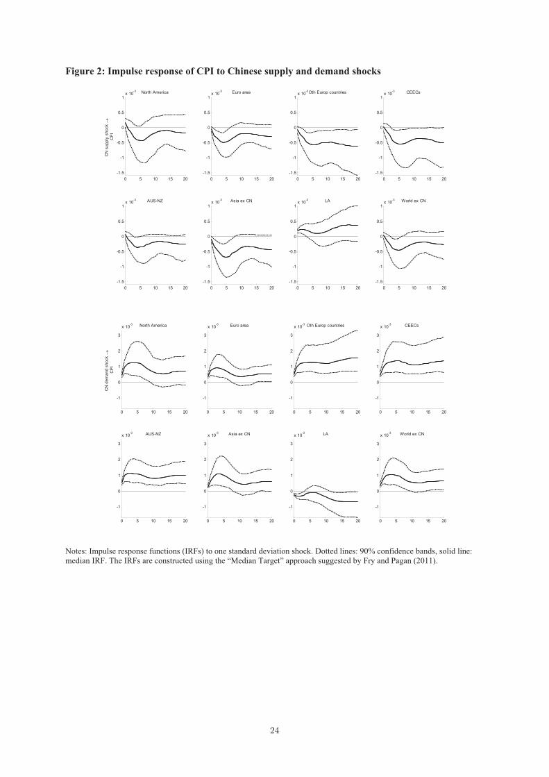
prices. After the Chinese supply shock, the CPI declines in almost every region by a
maximum of about 0.05 percent after three quarters (median effects). The effects are,
however, not significant in North America, and consumer prices in Latin America increase
temporarily. The effects on the PPI are even stronger. Producer prices decline by 0.2-0.4
percent; effects are particularly pronounced in Australia-New Zealand.
After the demand shock, the CPI rises significantly in each region with the exception of
Latin America. It reaches its maximum of about 0.1 percent after one year. Effects on the
CPI and the PPI are particularly strong in North America, Other European countries and
Australia-New Zealand. Producer prices do not change significantly or even turn negative
temporarily in the CEECs and Latin America.
The finding that the PPI reactions exceed those of the CPI reactions might be explained
by the PPI we use being mainly based on tradable manufactured goods. By contrast, in
the US, for example, services (excluding energy services) represent 56 percent of the basket
underlying the CPI according to the 2009-2010 CPI-U weights, with 31 percent referring
solely to the rent of shelter. Another reason could be that any impact on the producer level
(which is rather directly affected by external shocks) is not fully passed on to consumers
due to imperfect competition. The next sections shed light on the transmission mechanism.
Table 2 shows that Chinese supply shocks explain between 0.4 and 2 (between 1 and
5) percent of the forecast error of foreign consumer (producer) price inflation rates. The
percentage shares are particularly large in the euro area and Australasia, whereas they
are small in Latin America. Chinese demand shocks tend to explain a larger share than
Chinese supply shocks: between 1 percent (in Latin America) and 8 percent (in Other
European countries). The shares explained by global shocks are 6-33 percent for CPI
inflation and 7-38 percent for PPI inflation, with the bulk, again, accounted for by the
idiosyncratic component, which might reflect variable-specific, country-specific or regional
factors, broadly in line with the results of Osorio and Unsal (2011) for Australasia.
Overall, our results confirm the strong comovement of inflation rates across countries.9
However, Chinese shocks seem to be less important than other global shocks for foreign
inflation rates. Chinese demand shocks have dominated supply shocks as drivers of inter-
national price developments (with some difference across countries and price measures).
However, the difference between the contribution of supply and demand shocks is not
found to be large. This suggests that the relative size of supply and demand shocks will
determine whether deflationary or inflationary effects from China will prevail in the future.
5.3 Transmission mechanism I: Impulse responses of variables capturing
transmission channels
We now present impulse responses capturing the various transmission channels through
which supply and demand shocks in China can affect prices in other countries.10 It is
possible to distinguish between supply and demand-side channels, on the one hand, and
direct (trade-related) and indirect channels, on the other. The supply-side channel can
matter for inflation in other countries (directly) through effects on imported goods price
developments and (indirectly) through competitive pressures and by lowering margins and
bargaining powers in goods and labor markets. Another indirect supply effect would occur
if marginal costs increase as foreign producers change the composition of their products
9We obtain shares explained by global factors (or shocks) that are somewhat smaller than those found byCiccarelli and Mojon (2010), who use a similar factor model. This discrepancy is presumably attributableto our estimation of global factors from a much more heterogeneous dataset with different types of variables,whereas their dataset comprises only inflation rates.10Côté and de Resende (2008) provide a useful overview of the channels.
��
towards higher quality products. The demand channel can have a direct effect on foreign
inflation by raising demand for foreign goods and, hence, foreign export prices as well as
an indirect effect via higher commodity prices.
It is important to note that Chinese supply shocks may exert both supply-side and
demand-side effects abroad, and the same holds for Chinese demand shocks. For exam-
ple, Chinese supply shocks can lead to an increase in demand for foreign goods or for
commodities and therefore an increase in foreign export or commodity prices. Chinese
demand shocks, through raising demand for domestic goods, can lead to an increase in
foreign import prices which affects supply conditions abroad.
Which channel dominates and whether the overall impact of shocks in China on foreign
inflation is positive or negative ultimately need to be solved empirically.
When presenting our results, we differentiate between supply and demand channels,
on the one hand, and direct (trade-related) and indirect channels, on the other. We also
consider the reaction of monetary policy rates as well as the propagation of the shocks to
foreign GDP. Assessing the behavior of GDP after the shocks is interesting per se given
that the literature on business cycle linkages between China and the rest of the world is
still small. Moreover, a weakening or a strengthening of economic activity would imply
further downward or upward pressures on prices. We finally note upfront that our modeling
framework enables us to look at the effects of shocks on variables capturing the various
transmission channels, but not to assess how those changes, in turn, affect consumer and
producer price developments.
5.3.1 Transmission mechanism for Chinese supply shocks
Direct transmission The Chinese supply shock seems to be transmitted to foreign
prices directly via import prices (Figure 4), consistent, for example, with Feyziogulu and
Willard (2006), Kumar et al. (2003), Kamin et al. (2006) and Morel (2007). Import prices
decline significantly in all regions except for North America where they temporarily in-
crease (although not significantly). The decline is strongest in Australia-New Zealand
(more than 1 percent), followed by Asia and Latin America (both about 0.5 percent).
This suggests that the supply-side direct channel is effective.
The demand-side direct channel does, however, not seem to matter in the case of the
supply shock, as foreign export prices decline significantly in all regions. Higher Chinese
demand for foreign goods would have instead raised export prices.
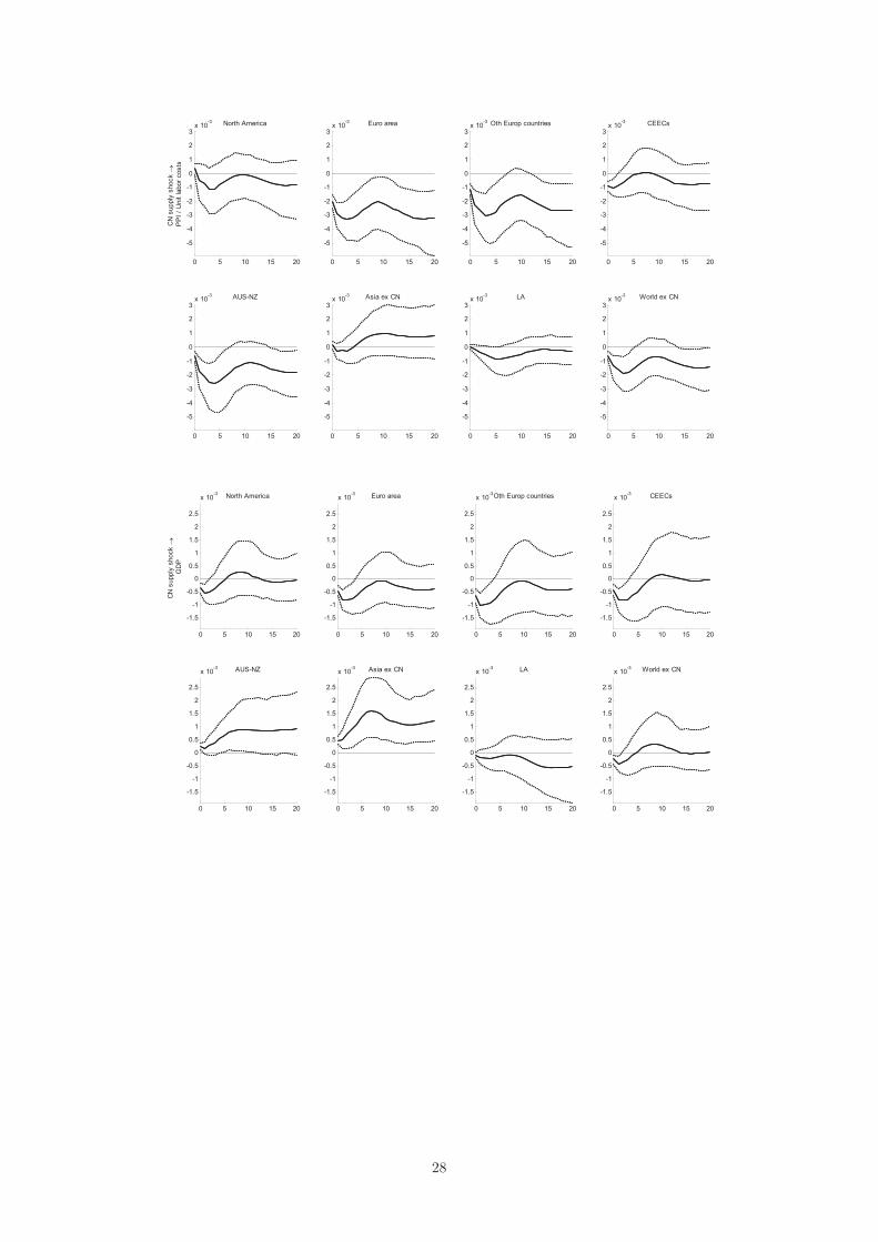
Indirect transmission The shock also tends to be transmitted indirectly (via com-
petitive pressures), which is consistent with Côté and de Resende (2008) who also find
this indirect supply channel to be effective and economically important. Unit labor costs
decline in Asia, Australia-New Zealand, North America and the CEECs. Effects are
��
strongest in Asia (almost -0.4 percent). We observe, however, a short-run increase in
the other regions. For Latin America, the rise in unit labor costs may have contributed
to the rise in the CPI. Similarly, real earnings increase in some countries and decline in
others. We recall that we look at aggregate Chinese supply shocks which comprise, e.g.,
technology, labor supply and markup shocks. This may help interpreting why responses of
earnings (and unit labor costs) differ across countries: Positive technology spillover effects
possibly exceed negative effects from competitive cost pressures in some countries, but not
in others. Another interpretation would be an increase in marginal costs due to a shift
towards higher quality products in some countries which would be consistent with Mandel
(2013).
We also consider producer prices relative to unit labor costs which reflects firms’ profit
margins. They go down in all regions, but the decline is not or only marginally significant
in North America, Asia and Latin America. For North America, an explanation might be
that goods and labor markets are more flexible than in other countries so that prices and
wages can adjust quickly.
GDP rises immediately and persistently after the Chinese supply shocks in Australia-
New Zealand and Asia, which are major suppliers of commodities and intermediate goods
to the Chinese economy. The effects are largest after about one year at 0.1 percent
and 0.15 percent, respectively. By contrast, GDP declines initially in all other regions,
exerting further downward pressures on foreign prices, and turns insignificant after less
than a year.11
Moreover, we observe a depreciation of currencies in real effective terms in North and
Latin America, and an appreciation and, thus, a worsening of price competitiveness in
the other regions.12 The depreciation in North America may explain why import prices
rise there as well (unlike in other regions). North America is typically seen as a large and
relatively closed economy, which cannot benefit much from international demand division.
Given a large US trade deficit over the entire sample period, a depreciation means a loss
of purchasing power and an even higher import bill, thereby dampening GDP.
Finally, monetary policy reacts by lowering interest rates (also relative to inflation)
clearly only in Australia-New Zealand, which counteracts the negative reaction of prices
to the Chinese supply shocks. Another factor countering the negative effects on prices
is the rise of commodity prices to the shocks. Prices of copper, energy and crude oil go
11We also note that the negative (Chinese against other countries’) GDP correlations are consistentwith the international real business cycle model of Backus, Kehoe and Kydland (1992). In this model,positive technology shocks in one country (China) lead to shifts of resources (capital and labor) to themore productive location (China in our case). Consequently, investment, employment and output mightdecrease in other countries. Similarly, Samuelson (2004) shows that productivity gains in one countrybrings about a permanent real income per capita loss for its trading partner.12We have replaced the real effective exchange rates with nominal effective exchange rates and re-
estimated our model. The responses of the nominal rates to Chinese supply and demand shocks are verysimilar to the responses of the real rates.
��
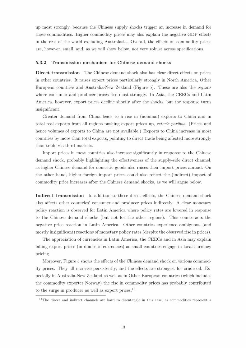
up most strongly, because the Chinese supply shocks trigger an increase in demand for
these commodities. Higher commodity prices may also explain the negative GDP effects
in the rest of the world excluding Australasia. Overall, the effects on commodity prices
are, however, small, and, as we will show below, not very robust across specifications.
5.3.2 Transmission mechanism for Chinese demand shocks
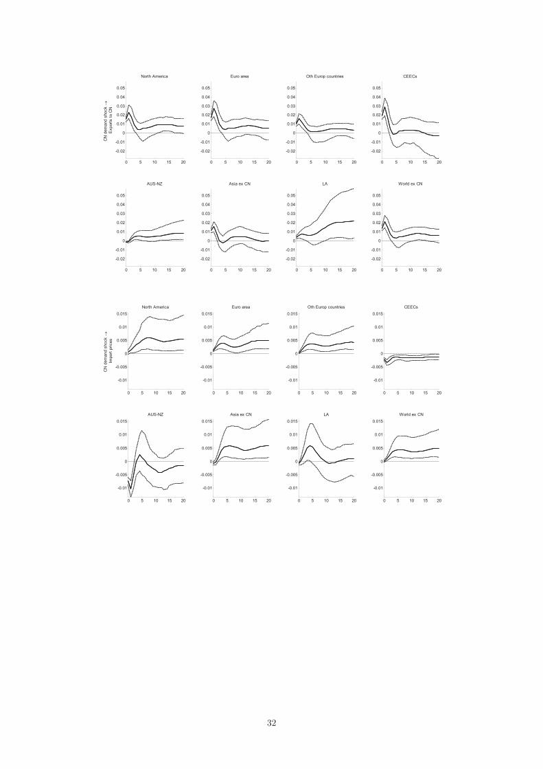
Direct transmission The Chinese demand shock also has clear direct effects on prices
in other countries. It raises export prices particularly strongly in North America, Other
European countries and Australia-New Zealand (Figure 5). These are also the regions
where consumer and producer prices rise most strongly. In Asia, the CEECs and Latin
America, however, export prices decline shortly after the shocks, but the response turns
insignificant.
Greater demand from China leads to a rise in (nominal) exports to China and in
total real exports from all regions pushing export prices up, ceteris paribus. (Prices and
hence volumes of exports to China are not available.) Exports to China increase in most
countries by more than total exports, pointing to direct trade being affected more strongly
than trade via third markets.
Import prices in most countries also increase significantly in response to the Chinese
demand shock, probably highlighting the effectiveness of the supply-side direct channel,
as higher Chinese demand for domestic goods also raises their import prices abroad. On
the other hand, higher foreign import prices could also reflect the (indirect) impact of
commodity price increases after the Chinese demand shocks, as we will argue below.
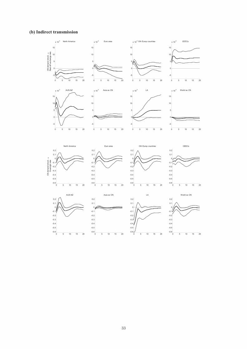
Indirect transmission In addition to these direct effects, the Chinese demand shock
also affects other countries’ consumer and producer prices indirectly. A clear monetary
policy reaction is observed for Latin America where policy rates are lowered in response
to the Chinese demand shocks (but not for the other regions). This counteracts the
negative price reaction in Latin America. Other countries experience ambiguous (and
mostly insignificant) reactions of monetary policy rates (despite the observed rise in prices).
The appreciation of currencies in Latin America, the CEECs and in Asia may explain
falling export prices (in domestic currencies) as small countries engage in local currency
pricing.
Moreover, Figure 5 shows the effects of the Chinese demand shock on various commod-
ity prices. They all increase persistently, and the effects are strongest for crude oil. Es-
pecially in Australia-New Zealand as well as in Other European countries (which includes
the commodity exporter Norway) the rise in commodity prices has probably contributed
to the surge in producer as well as export prices.13
13The direct and indirect channels are hard to disentangle in this case, as commodities represent a
��
The latter finding is interesting from two points of view. First, the rise in the price
of all commodities after the Chinese demand shock is about ten times greater than the
rise in Chinese consumer or producer prices.14 This suggests that the demand increase
is distributed very unevenly across goods and much of it is directed to commodities.
Second, Kilian (2009) shows that world aggregate demand shocks are the major drivers
of world oil prices. We confirm here that Chinese demand shocks have a strong impact
on oil prices. Variance decompositions for commodity price inflation suggest that Chinese
demand and supply shocks explain roughly 12 percent of the forecast error variance of
crude oil price inflation (the bulk (10 percent) is explained by Chinese demand shocks)
and 11 percent of movements of all commodities’ prices (Table 2). Shocks to the global
factors account for more than 20 percent of the variation in the forecast error of both
crude oil and all commodity price inflation. The rest is explained by idiosyncratic factors
which, for commodity price inflation, comprise commodity-specific supply and demand
shocks and regional- or country-specific shocks. The share explained by Chinese shocks
we obtain is consistent with Roache (2012). That study finds, based on a structural VAR
estimated over 2000-2011, that Chinese activity shocks account for roughly 7 percent of
the variation in world oil prices (and slightly less of the variation in other commodity
prices). Our finding regarding the decomposition of oil price developments is also not
inconsistent with Aastveit et al. (2012). The share of oil price fluctuations explained by
Chinese shocks estimated by us is a bit smaller than the one explained by demand shocks
from a larger number of emerging economies, mostly from emerging Asia, estimated by
Aastveit et al. (2012) at about 30 percent.
The rise in world commodity prices has probably prevented a positive reaction of GDP
in most countries. The Chinese demand shocks are transmitted positively and significantly
to GDP only in Australia-New Zealand and Latin America which are commodity net
exporters, and in Asia which is a commodity net importer, but where positive trade
effects seem to have dominated the negative effects on GDP stemming from commodity
prices. Hence, the demand shocks from China also display positive demand effects in the
surrounding regions, which have probably pushed prices further upward in these regions.
In Latin America, as prices went down, interest rates decreased as well, which can also
help explain the positive GDP effect in this region. We note that our estimated foreign
GDP effects after Chinese demand shocks are very similar to the GVAR results for Chinese
"output shocks" by Feldkircher and Korhonen (2012).15
sizeable portion of overall exports.14Osorio and Unsal (2011) also find an effect (after two quarters) of a Chinese GDP shock on commodity
prices which is larger than on consumer prices, although the difference is much smaller than in our case.While commodity prices in their analysis are affected with a time lag, ours react instantaneously to theChinese demand shocks.15We have also carried out variance decompositions of GDP growth. Chinese demand shocks are more
important than supply shocks for all regions. The shares explained by Chinese shocks are between 2
��
The overall message from this section is that both Chinese supply and demand shocks
and channels and both direct and indirect transmission channels seem to matter for infla-
tion in other countries. As byproducts, we find that Chinese shocks account for 11 percent
(4 percent) of fluctuations in commodity prices (foreign GDP).
5.4 Transmission mechanism II: Relating price impulse responses to
country characteristics
In this section, we exploit the cross-section dimension and relate CPI and PPI impulse
responses of individual countries to country characteristics in order to shed more light on
the transmission channels. We carry out bivariate OLS and robust regressions (to correct
for outliers) of impulse responses of all 37 countries (if available) one year after the Chinese
supply and demand shocks on the following determinants: openness (defined as the sum
of exports and imports relative to GDP), imports from and exports to China relative
to GDP, commodity imports and exports relative to GDP, manufacturing value added
relative to GDP, distance of the capital city from Beijing, product market regulation,
(regular) employment protection, structural similarity with China. Manufacturing value
added and distance are taken from the World Bank World Development Indicators and
from the CEPII GeoDist database, respectively. The regulatory variables are taken from
OECD (2012) and are measured for 2008 on an index scale of 0-6 from least to most
restrictive.16 The structural similarity of a country j with China is defined as Sj =∑Ll=1 |slj − slCN |, where slj and slCN denote the shares of sector l in total exports of
country j and China, respectively (see Krugman (1991)).17 Small values indicate greater
structural similarity. The sectors correspond to the groups of goods at the two-digit level
of the SITC classification system. The similarity measure is constructed for 2006, and
underlying data were taken from the UN Comtrade database.
In Table 3 we show the signs of the significant regression coefficients together with the
level of significance. Significant correlations of the trade and commodity price exposure
measures, distance, the manufacturing share and product market regulation with the price
impulse responses have the expected signs (with the exception of distance with the PPI
impulse response functions to the supply shock obtained from the OLS regression). I.e. the
percent (in Latin America) and 6 percent (in North America and Other European countries).16The indicator of product market regulation measures the degree to which policies promote or inhibit
competition in areas of the product market where competition is viable. It covers formal regulations in thefollowing areas: state control of business enterprises; legal and administrative barriers to entrepreneurship;and barriers to international trade and investment. The indicator of employment protection measuresthe procedures and costs involved in dismissing workers with regular contracts and incorporates severalbasic measures of employment protection strictness, such as notice periods, amount of severance pay andcompensation for unfair dismissal.17Typically, this measure is constructed using disaggregated value added figures which are, however, not
available for our reference country China. Therefore, we use export data which are also more useful forderiving implications of competition with China on international markets.
��
larger the trade and commodity exposure and the manufacturing sector and the smaller the
distance to Beijing are, the stronger the price response after Chinese shocks. The table also
shows that producer price reactions in a country with a sectoral export structure that is
similar to China’s export structure will be relatively weak after Chinese shocks. Producers
from countries which compete with China appear not to raise prices after positive demand
shocks or negative supply shocks as much as producers from countries which have a very
different export structure compared to and therefore do not compete with China. At the
same time, due to low markups producers from countries that compete with China cannot
lower prices by as much as producers from countries that compete less with China after
negative demand or positive supply shocks.
Overall, we conclude from this section that overall trade exposure, direct trade with
China, commodity exposure and, to a less robust extent, the manufacturing share, distance
and structural similarity with China help to explain differences across countries in price
reactions to the Chinese supply and demand shocks.18 The regulatory measures in general
do not enter the regression equations significantly. The findings from this section that trade
and commodity prices are important transmission channels are consistent with section 5.3.
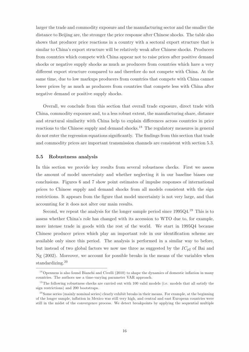
5.5 Robustness analysis
In this section we provide key results from several robustness checks. First we assess
the amount of model uncertainty and whether neglecting it in our baseline biases our
conclusions. Figures 6 and 7 show point estimates of impulse responses of international
prices to Chinese supply and demand shocks from all models consistent with the sign
restrictions. It appears from the figure that model uncertainty is not very large, and that
accounting for it does not alter our main results.
Second, we repeat the analysis for the longer sample period since 1995Q4.19 This is to
assess whether China’s role has changed with its accession to WTO due to, for example,
more intense trade in goods with the rest of the world. We start in 1995Q4 because
Chinese producer prices which play an important role in our identification scheme are
available only since this period. The analysis is performed in a similar way to before,
but instead of two global factors we now use three as suggested by the ICp2 of Bai and
Ng (2002). Moreover, we account for possible breaks in the means of the variables when
standardizing.20
18Openness is also found Bianchi and Civelli (2010) to shape the dynamics of domestic inflation in manycountries. The authors use a time-varying parameter VAR approach.19The following robustness checks are carried out with 100 valid models (i.e. models that all satisfy the
sign restrictions) and 200 bootstraps.20Some series (mainly nominal series) clearly exhibit breaks in their means. For example, at the beginning
of the longer sample, inflation in Mexico was still very high, and central and east European countries werestill in the midst of the convergence process. We detect breakpoints by applying the sequential multiple
��
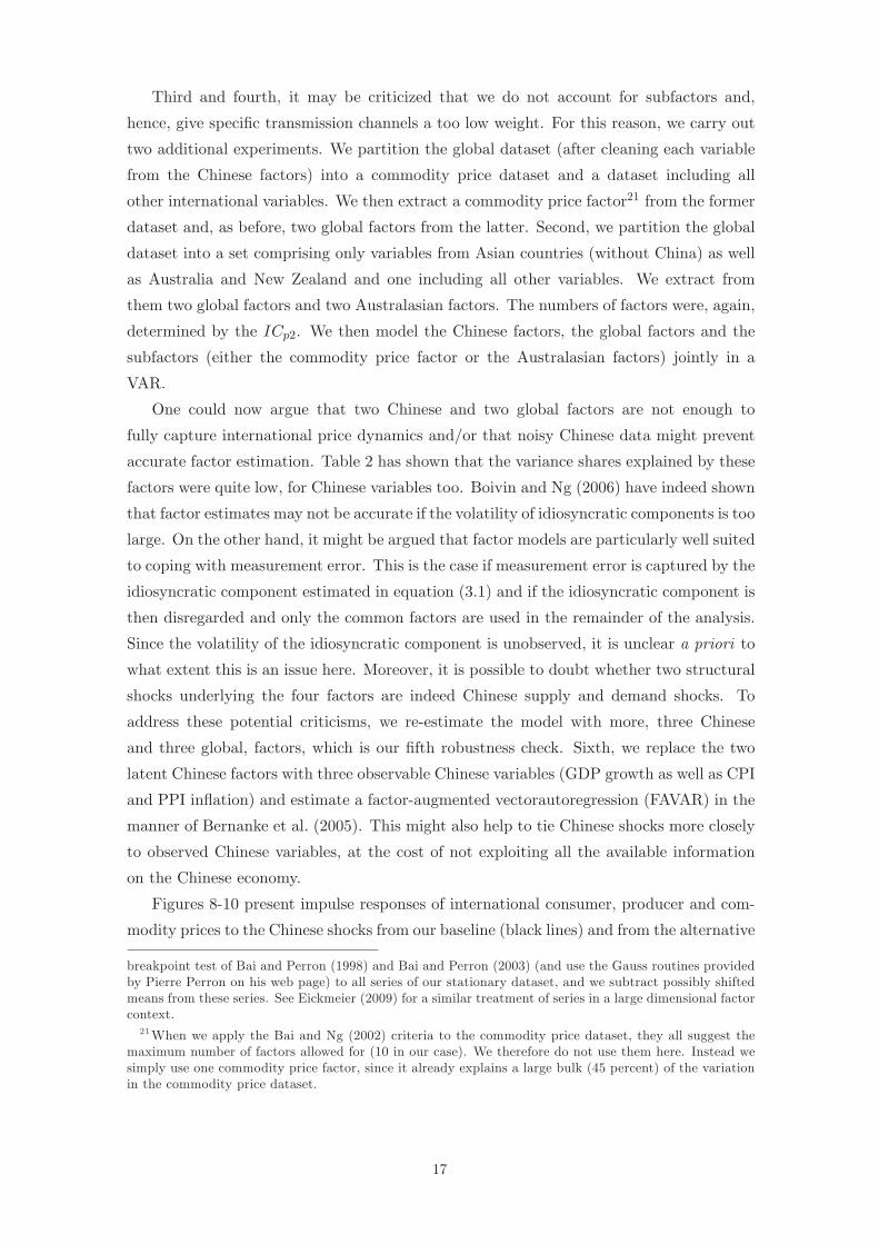
Third and fourth, it may be criticized that we do not account for subfactors and,
hence, give specific transmission channels a too low weight. For this reason, we carry out
two additional experiments. We partition the global dataset (after cleaning each variable
from the Chinese factors) into a commodity price dataset and a dataset including all
other international variables. We then extract a commodity price factor21 from the former
dataset and, as before, two global factors from the latter. Second, we partition the global
dataset into a set comprising only variables from Asian countries (without China) as well
as Australia and New Zealand and one including all other variables. We extract from
them two global factors and two Australasian factors. The numbers of factors were, again,
determined by the ICp2. We then model the Chinese factors, the global factors and the
subfactors (either the commodity price factor or the Australasian factors) jointly in a
VAR.
One could now argue that two Chinese and two global factors are not enough to
fully capture international price dynamics and/or that noisy Chinese data might prevent
accurate factor estimation. Table 2 has shown that the variance shares explained by these
factors were quite low, for Chinese variables too. Boivin and Ng (2006) have indeed shown
that factor estimates may not be accurate if the volatility of idiosyncratic components is too
large. On the other hand, it might be argued that factor models are particularly well suited
to coping with measurement error. This is the case if measurement error is captured by the
idiosyncratic component estimated in equation (3.1) and if the idiosyncratic component is
then disregarded and only the common factors are used in the remainder of the analysis.
Since the volatility of the idiosyncratic component is unobserved, it is unclear a priori to
what extent this is an issue here. Moreover, it is possible to doubt whether two structural
shocks underlying the four factors are indeed Chinese supply and demand shocks. To
address these potential criticisms, we re-estimate the model with more, three Chinese
and three global, factors, which is our fifth robustness check. Sixth, we replace the two
latent Chinese factors with three observable Chinese variables (GDP growth as well as CPI
and PPI inflation) and estimate a factor-augmented vectorautoregression (FAVAR) in the
manner of Bernanke et al. (2005). This might also help to tie Chinese shocks more closely
to observed Chinese variables, at the cost of not exploiting all the available information
on the Chinese economy.
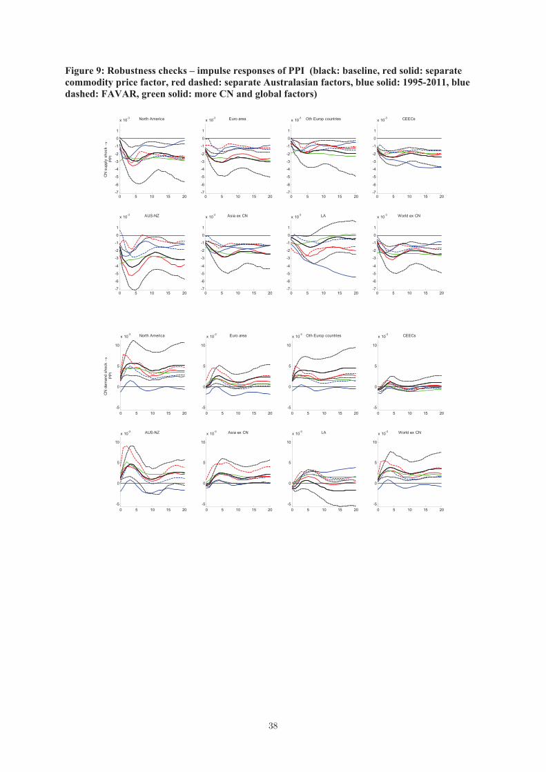
Figures 8-10 present impulse responses of international consumer, producer and com-
modity prices to the Chinese shocks from our baseline (black lines) and from the alternative
breakpoint test of Bai and Perron (1998) and Bai and Perron (2003) (and use the Gauss routines providedby Pierre Perron on his web page) to all series of our stationary dataset, and we subtract possibly shiftedmeans from these series. See Eickmeier (2009) for a similar treatment of series in a large dimensional factorcontext.21When we apply the Bai and Ng (2002) criteria to the commodity price dataset, they all suggest the
maximum number of factors allowed for (10 in our case). We therefore do not use them here. Instead wesimply use one commodity price factor, since it already explains a large bulk (45 percent) of the variationin the commodity price dataset.
��
experiments (red solid lines: separate commodity price factor, red dashed: separate Aus-
tralasian factors, blue solid: 1995-2011 sample period, blue dashed: FAVAR, green solid:
more (three Chinese and three global) factors). For visibility, we show only median im-
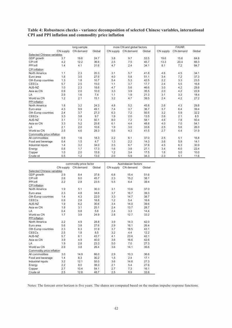
pulse response functions for the robustness checks. Table 4 provides the corresponding
variance decompositions.
Overall, our main results are not much affected. The median impulse responses of the
robustness checks in most cases lie within the confidence bands of impulse responses from
the baseline. A few differences from the baseline are, however, worth mentioning.
First, responses of prices after Chinese demand shocks and of commodity prices after
both supply and demand shocks, in general, turn out to be weaker when the model is
estimated over the longer sample period. This suggests that, with greater integration of
China into the world economy (related to its accession to the WTO), the transmission
of Chinese demand shocks to other countries has strengthened, and that this is (at least
partly) due to greater demand for commodities from China.
Second, when separate Australasian factors are included in the model, the effects of
Chinese demand shocks on foreign consumer prices are slightly stronger than in the base-
line. This is also visible from the variance decomposition presented in Table 4. Variance
shares explained by Chinese demand shocks now increase to more than 10 percent on
average over all countries (compared to 4 percent in the baseline). This suggests that
the shock transmission from China to the rest of the world goes partially through Aus-
tralasia. Differences are, however, unlikely to be significant since confidence bands will
overlap. We nevertheless believe that accounting for factors which only load on subsets
of our large global dataset is a promising route to follow in future work (see, for example,
Aastveit et al. (2012) and Foerster and Tillmann (2013) for insightful applications of such
approaches in the global inflation context).
Third, the finding from our baseline that commodity prices rise after the Chinese
supply shock (although we found them to rise only to a small extent) does not seem to
be very robust. It is indeed not fully clear whether supply shocks in China will result in
greater demand for commodities or whether commodities will instead be substituted as
production becomes more capital and technology-intensive.
Fourth, the FAVAR suggests a somewhat weaker (but probably not significantly differ-
ent) short-term reaction by producer prices to the supply shock in most regions. Fifth, in
the FAVAR, the forecast error variance of Chinese variables is, by construction, entirely ac-
counted for by contributions from Chinese supply and demand shocks and global shocks.
Chinese supply shocks now explain 20 percent of Chinese GDP growth and between 8
and 13 percent of inflation. The contribution of Chinese demand shocks on Chinese vari-
ables also increases relative to the baseline, albeit not by as much. The remaining shocks
(probably mostly global shocks) are still the dominant driving force of Chinese variables.
Variance shares for foreign inflation rates are not much altered compared with the baseline
�
model. Overall, we conclude that our main results are fairly robust.
6 Concluding remarks
We apply a structural dynamic factor model to a large quarterly dataset covering 38 coun-
tries (including China) between 2002 and 2011 to analyze China’s role in global inflation
dynamics. We identify Chinese supply and demand shocks and examine their contribu-
tions to foreign price dynamics and their transmission channels. Our contributions to the
literature are that we focus on identified Chinese shocks and that we account for interac-
tion between many variables in our model, which allows us to analyze the transmission
mechanism in great detail. Our main findings are: (i) Chinese supply and demand shocks
significantly affect prices in other countries. Demand shocks matter slightly more over
the sample period than supply shocks. Producer prices tend to be more strongly affected
than consumer prices by Chinese shocks. The overall share of international inflation ex-
plained by Chinese shocks is notable (about 5 percent on average over all countries but not
more than 13 percent in each region). This suggests that monetary policy makers should
take macroeconomic developments in China into account when stabilizing domestic infla-
tion rates; (ii) Direct channels (via import and export prices) and indirect channels (via
greater exposure to foreign competition and commodity prices) both seem to matter; (iii)
Differences in trade (overall and with China) and in commodity exposure help explaining
cross-country differences in price responses.
References
Aastveit, K., Bjoernland, H. and Thorsrud, L. (2012), ‘What drives oil prices? Emerging
versus developed economies’, Mimeo, Norges Bank .
ADB (2011), ‘Asian Development Outlook’, p. 23.
Backus, D., Kehoe, P. and Kydland, F. (1992), ‘International real business cycles’, Journal
of Political Economy 100(4), 745—775.
Bai, J. and Ng, S. (2002), ‘Determining the number of factors in approximate factor
models’, Econometrica 70(1), 191—221.
Bai, J. and Perron, P. (1998), ‘Estimating and testing linear models with multiple struc-
tural changes’, Econometrica 66, 47—78.
Bai, J. and Perron, P. (2003), ‘Computation and analysis of multiple structural change
models’, Journal of Applied Econometrics 18, 1—22.
�
Bernanke, B., Boivin, J. and Eliasz, P. (2005), ‘Measuring the effects of monetary policy:
a factor-augmented vector autoregressive (FAVAR) approach’, The Quarterly Journal
of Economics 120(1), 387.
Bianchi, F. and Civelli, A. (2010), ‘A structural approach to the globalization hypothesis
for national inflation rates’, Mimeo, Duke University .
Boivin, J. and Ng, S. (2006), ‘Are more data always better for factor analysis?’, Journal
of Econometrics 132(1), 169—194.
Borio, C. and Filardo, A. (2007), ‘Globalization and inflation: new cross-country evidence
on the global determinants of domestic inflation’, BIS Working Paper 227.
Cesa-Bianchi, A., Pesaran, H., Rebucci, A. and Xu, T. (forthcoming), ‘China’s emergence
in the world economy and business cycles’, Economia, Journal of the Latin American
and Caribbean Economic Association .
Chamberlain, G. and Rothschild, M. (1983), ‘Arbitrage, factor structure, and mean-
variance analysis on large asset markets’, Econometrica 51(5), 1281—1304.
Ciccarelli, M. and Mojon, B. (2010), ‘Global inflation’, Review of Economics and Statistics
92(3), 524—535.
Côté, D. and de Resende, C. (2008), ‘Globalization and inflation: the role of China’, Bank
of Canada Working Paper 2008-35.
Eickmeier, S. (2009), ‘Comovements and heterogeneity in the euro area analyzed in a
non-stationary factor dynamic model’, Journal of Applied Econometrics 24, 933—959.
Eickmeier, S. and Ng, T. (2011), ‘How do credit supply shocks propagate internationally?
A GVAR approach’, CEPR Discussion Paper 8720.
Eickmeier, S. and Pijnenburg, K. (2013), ‘The global dimension of inflation - evidence
from factor-augmented Phillips curves’, Oxford Bulletin of Economics and Statistics
74, 103—122.
Farrant, K. and Peersman, G. (2006), ‘Is the exchange rate a shock absorber or a source
of shocks? New empirical evidence’, Journal of Money, Credit and Banking 38(4), 939—
961.
Feldkircher, M. and Korhonen, I. (2012), ‘The rise of China and its implications for emerg-
ing markets - evidence from a GVAR model’, Bank of Finland Discussion Paper 20.
Feyziogulu, T. and Willard, L. (2006), ‘Does inflation in China affect the United States
and Japan’, IMF Working Paper 06/36.
��
Foerster, M. and Tillmann, P. (2013), ‘Local inflation. reconsidering the international
comovement of inflation’, MAGKS Joint Discussion Paper Series 03-2013.
Forni, M., Hallin, M., Lippi, M. and Reichlin, L. (2000), ‘The generalized dynamic-factor
model: identification and estimation’, Review of Economics and Statistics 82(4), 540—
554.
Fry, R. and Pagan, A. (2007), ‘Some issues in using sign restrictions for identifying struc-
tural VARs’, NCER Working Paper 14.
Fry, R. and Pagan, A. (2011), ‘Sign restrictions in structural vector autoregressions: a
critical review’, Journal of Economic Literature 49(4), 938—960.
Furlanetto, F., Ravazzolo, F. and Sarferaz, S. (2012), ‘Identification of financial factors in
economic fluctuations’, Mimeo, Norges Bank .
Kamin, S., Marazzi, M. and Schindler, J. (2006), ‘The impact of Chinese exports on global
import prices’, Review of International Economics 14(2), 179—201.
Kilian, L. (1997), ‘Small-sample confidence intervals for impulse response functions’, Re-
view of Economics and Statistics 80(2), 218—230.
Kilian, L. (2009), ‘Not all oil price shocks are alike: disentangling demand and supply
shocks in the crude oil market’, American Economic Review 99(3), 1053—1069.
Krugman, P. (1991), Geography and trade, MIT Press, Cambridge.
Kumar, M., Taimur, B., Decressin, J., MacDonagh, C. and Feyziogulu, T. (2003), ‘Defla-
tion: determinants, risks, and policy-option-findings of an interdepartmental task force’,
IMF Occasional Paper 221.
Li, H., Li, L., Wu, B. and Xiong, Y. (2012), ‘The end of cheap Chinese labor’, Journal of
Economic Perspectives 26(4), 57—74.
Mandel, B. (2013), ‘Chinese exports and U.S. import prices’, Federal Reserve Bank of New
York Staff Reports 591.
Morel, L. (2007), ‘The direct effect of China on Canadian consumer prices: an empirical
assessment’, Bank of Canada Discussion Paper 10.
Mumtaz, H. and Surico, P. (forthcoming), ‘Evolving international inflation dynamics:
world and country-specific factors’, Journal of the European Economic Association .
Osorio, C. and Unsal, D. (2011), ‘Inflation dynamics in Asia: causes, changes, and
spillovers from China’, IMF Working Paper 11/257.
��
Peersman, G. (2005), ‘What caused the early millenium slowdown? Evidence based on
vector autoregressions’, Journal of Applied Econometrics 20, 185—207.
Roache, S. (2012), ‘China’s impact on world commodity markets’, IMF Working Paper
12/115.
Rubio-Ramírez, J., Waggoner, D. and Zha, T. (2010), ‘Structural vector autoregres-
sions: theory of identification and algorithms for inference’, Review of Economic Studies
77(2), 665—696.
Samuelson, P. (2004), ‘Where Ricardo and Mill rebut and confirm arguments of
mainstream economists supporting globalization’, Journal of Economic Perspectives
18(3), 135—146.
Smets, F. and Wouters, R. (2003), ‘An estimated dynamics stochastic general equilibrium
model of the euro area’, Journal of the European Economic Association 1(5), 1123—1175.
Song, Z., Storesletten, K. and Zilibotti, F. (2011), ‘Growing like China’, American Eco-
nomic Review 101, 202—241.
Stock, J. and Watson, M. (2002a), ‘Forecasting using principal components from a large
number of predictors’, Journal of the American Statistical Association 97(460), 1167—
1179.
Stock, J. and Watson, M. (2002b), ‘Macroeconomic forecasting using diffusion indexes’,
Journal of Business & Economic Statistics 20(2), 147.
Stock, J. andWatson, M. (2005), ‘Implications of dynamic factor models for VAR analysis’,
NBER Working Paper 11467.
Zhu, X. (2012), ‘Understanding China’s growth: past, present, and future’, Journal of
Economic Perspectives 26(4), 103—124.
��
Figure 1: Impulse responses of selected Chinese variables to Chinese supply and demand shocks
Notes: Impulse response functions (IRFs) to one standard deviation shock. Dotted lines: 90% confidence bands, solid line: median IRF. The IRFs are constructed using the “Median Target” approach suggested by Fry and Pagan (2011).
0 5 10 15 200
0.5
1
1.5
2
2.5x 10
-3 GDP
CN
sup
ply
shoc
k
0 5 10 15 20
-2.5
-2
-1.5
-1
-0.5
0
x 10-3 CPI
0 5 10 15 20-5
-4
-3
-2
-1
0x 10
-3 PPI
0 5 10 15 20
-1
0
1
2
3
x 10-3 GDP
CN
dem
and
shoc
k
0 5 10 15 200
1
2
3
4
5
x 10-3 CPI
0 5 10 15 200
2
4
6
8
x 10-3 PPI
��
Figure 2: Impulse response of CPI to Chinese supply and demand shocks
Notes: Impulse response functions (IRFs) to one standard deviation shock. Dotted lines: 90% confidence bands, solid line: median IRF. The IRFs are constructed using the “Median Target” approach suggested by Fry and Pagan (2011).
0 5 10 15 20-1.5
-1
-0.5
0
0.5
1x 10
-3 North America
CN
sup
ply
shoc
k �
C
PI
0 5 10 15 20-1.5
-1
-0.5
0
0.5
1x 10
-3 Euro area
0 5 10 15 20-1.5
-1
-0.5
0
0.5
1x 10
-3Oth Europ countries
0 5 10 15 20-1.5
-1
-0.5
0
0.5
1x 10
-3 CEECs
0 5 10 15 20-1.5
-1
-0.5
0
0.5
1x 10⁻³ AUS-NZ
0 5 10 15 20-1.5
-1
-0.5
0
0.5
1x 10⁻³ Asia ex CN
0 5 10 15 20-1.5
-1
-0.5
0
0.5
1x 10⁻³ LA
0 5 10 15 20-1.5
-1
-0.5
0
0.5
1x 10⁻³ World ex CN
0 5 10 15 20
-1
0
1
2
3
x 10-3 North America
CN
dem
and
shoc
k �
C
PI
0 5 10 15 20
-1
0
1
2
3
x 10-3 Euro area
0 5 10 15 20
-1
0
1
2
3
x 10-3 Oth Europ countries
0 5 10 15 20
-1
0
1
2
3
x 10-3 CEECs
0 5 10 15 20
-1
0
1
2
3
x 10-3 AUS-NZ
0 5 10 15 20
-1
0
1
2
3
x 10-3 Asia ex CN
0 5 10 15 20
-1
0
1
2
3
x 10-3 LA
0 5 10 15 20
-1
0
1
2
3
x 10-3 World ex CN
��
Figure 3: Impulse response of PPI to Chinese supply and demand shocks
Notes: Impulse response functions (IRFs) to one standard deviation shock. Dotted lines: 90% confidence bands, solid line: median IRF. The IRFs are constructed using the “Median Target” approach suggested by Fry and Pagan (2011).
0 5 10 15 20-7
-6
-5
-4
-3
-2
-1
0
1
x 10-3 North America
CN
sup
ply
shoc
k �
P
PI
0 5 10 15 20-7
-6
-5
-4
-3
-2
-1
0
1
x 10-3 Euro area
0 5 10 15 20-7
-6
-5
-4
-3
-2
-1
0
1
x 10-3 Oth Europ countries
0 5 10 15 20-7
-6
-5
-4
-3
-2
-1
0
1
x 10-3 CEECs
0 5 10 15 20-7
-6
-5
-4
-3
-2
-1
0
1
x 10-3 AUS-NZ
0 5 10 15 20-7
-6
-5
-4
-3
-2
-1
0
1
x 10-3 Asia ex CN
0 5 10 15 20-7
-6
-5
-4
-3
-2
-1
0
1
x 10-3 LA
0 5 10 15 20-7
-6
-5
-4
-3
-2
-1
0
1
x 10-3 World ex CN
0 5 10 15 20-5
0
5
10
x 10-3 North America
CN
dem
and
shoc
k �
P
PI
0 5 10 15 20-5
0
5
10
x 10-3 Euro area
0 5 10 15 20-5
0
5
10
x 10-3 Oth Europ countries
0 5 10 15 20-5
0
5
10
x 10-3 CEECs
0 5 10 15 20-5
0
5
10
x 10-3 AUS-NZ
0 5 10 15 20-5
0
5
10
x 10-3 Asia ex CN
0 5 10 15 20-5
0
5
10
x 10-3 LA
0 5 10 15 20-5
0
5
10
x 10-3 World ex CN
��
Figure 4: Transmission of Chinese supply shocks to selected international variables
(a) Direct (trade related) transmission
0 5 10 15 20
-15
-10
-5
0
x 10-3 North America
CN
sup
ply
shoc
k �
Im
port
pric
es
0 5 10 15 20
-15
-10
-5
0
x 10-3 Euro area
0 5 10 15 20
-15
-10
-5
0
x 10-3 Oth Europ countries
0 5 10 15 20
-15
-10
-5
0
x 10-3 CEECs
0 5 10 15 20
-15
-10
-5
0
x 10-3 AUS-NZ
0 5 10 15 20
-15
-10
-5
0
x 10-3 Asia ex CN
0 5 10 15 20
-15
-10
-5
0
x 10-3 LA
0 5 10 15 20
-15
-10
-5
0
x 10-3 World ex CN
0 5 10 15 20-16
-14
-12
-10
-8
-6
-4
-2
x 10-3 North America
CN
sup
ply
shoc
k �
E
xpor
t pric
es
0 5 10 15 20-16
-14
-12
-10
-8
-6
-4
-2
x 10-3 Euro area
0 5 10 15 20-16
-14
-12
-10
-8
-6
-4
-2
x 10-3 Oth Europ countries
0 5 10 15 20-16
-14
-12
-10
-8
-6
-4
-2
x 10-3 CEECs
0 5 10 15 20-16
-14
-12
-10
-8
-6
-4
-2
x 10-3 AUS-NZ
0 5 10 15 20-16
-14
-12
-10
-8
-6
-4
-2
x 10-3 Asia ex CN
0 5 10 15 20-16
-14
-12
-10
-8
-6
-4
-2
x 10-3 LA
0 5 10 15 20-16
-14
-12
-10
-8
-6
-4
-2
x 10-3 World ex CN
��
(b) Indirect transmission
0 5 10 15 20-6
-5
-4
-3
-2
-1
0
1
2x 10
-3 North America
CN
sup
ply
shoc
k �
U
nit l
abor
cos
ts
0 5 10 15 20-6
-5
-4
-3
-2
-1
0
1
2x 10
-3 Euro area
0 5 10 15 20-6
-5
-4
-3
-2
-1
0
1
2x 10
-3 Oth Europ countries
0 5 10 15 20-6
-5
-4
-3
-2
-1
0
1
2x 10
-3 CEECs
0 5 10 15 20-6
-5
-4
-3
-2
-1
0
1
2x 10⁻³ AUS-NZ
0 5 10 15 20-6
-5
-4
-3
-2
-1
0
1
2x 10⁻³ Asia ex CN
0 5 10 15 20-6
-5
-4
-3
-2
-1
0
1
2x 10⁻³ LA
0 5 10 15 20-6
-5
-4
-3
-2
-1
0
1
2x 10⁻³ World ex CN
0 5 10 15 20
-1
0
1
2
3
4
5
x 10-3 North America
CN
sup
ply
shoc
k �
E
arni
ngs
0 5 10 15 20
-1
0
1
2
3
4
5
x 10-3 Euro area
0 5 10 15 20
-1
0
1
2
3
4
5
x 10-3 Oth Europ countries
0 5 10 15 20
-1
0
1
2
3
4
5
x 10-3 CEECs
0 5 10 15 20
-1
0
1
2
3
4
5
x 10-3 AUS-NZ
0 5 10 15 20
-1
0
1
2
3
4
5
x 10-3 Asia ex CN
0 5 10 15 20
-1
0
1
2
3
4
5
x 10-3 LA
0 5 10 15 20
-1
0
1
2
3
4
5
x 10-3 World ex CN
��
0 5 10 15 20
-5
-4
-3
-2
-1
0
1
2
3x 10
-3 North America
CN
sup
ply
shoc
k �
P
PI /
Uni
t lab
or c
osts
0 5 10 15 20
-5
-4
-3
-2
-1
0
1
2
3x 10
-3 Euro area
0 5 10 15 20
-5
-4
-3
-2
-1
0
1
2
3x 10
-3 Oth Europ countries
0 5 10 15 20
-5
-4
-3
-2
-1
0
1
2
3x 10
-3 CEECs
0 5 10 15 20
-5
-4
-3
-2
-1
0
1
2
3x 10⁻³ AUS-NZ
0 5 10 15 20
-5
-4
-3
-2
-1
0
1
2
3x 10⁻³ Asia ex CN
0 5 10 15 20
-5
-4
-3
-2
-1
0
1
2
3x 10⁻³ LA
0 5 10 15 20
-5
-4
-3
-2
-1
0
1
2
3x 10⁻³ World ex CN
0 5 10 15 20
-1.5
-1
-0.5
0
0.5
1
1.5
2
2.5
x 10-3 North America
CN
sup
ply
shoc
k �
G
DP
0 5 10 15 20
-1.5
-1
-0.5
0
0.5
1
1.5
2
2.5
x 10-3 Euro area
0 5 10 15 20
-1.5
-1
-0.5
0
0.5
1
1.5
2
2.5
x 10-3Oth Europ countries
0 5 10 15 20
-1.5
-1
-0.5
0
0.5
1
1.5
2
2.5
x 10-3 CEECs
0 5 10 15 20
-1.5
-1
-0.5
0
0.5
1
1.5
2
2.5
x 10-3 AUS-NZ
0 5 10 15 20
-1.5
-1
-0.5
0
0.5
1
1.5
2
2.5
x 10-3 Asia ex CN
0 5 10 15 20
-1.5
-1
-0.5
0
0.5
1
1.5
2
2.5
x 10-3 LA
0 5 10 15 20
-1.5
-1
-0.5
0
0.5
1
1.5
2
2.5
x 10-3 World ex CN
�
0 5 10 15 20
-5
0
5
10
15
x 10-3 North America
CN
sup
ply
shoc
k �
R
eal e
ff ex
chan
ge ra
te
0 5 10 15 20
-5
0
5
10
15
x 10-3 Euro area
0 5 10 15 20
-5
0
5
10
15
x 10-3 Oth Europ countries
0 5 10 15 20
-5
0
5
10
15
x 10-3 CEECs
0 5 10 15 20
-5
0
5
10
15
x 10-3 AUS-NZ
0 5 10 15 20
-5
0
5
10
15
x 10-3 Asia ex CN
0 5 10 15 20
-5
0
5
10
15
x 10-3 LA
0 5 10 15 20
-5
0
5
10
15
x 10-3 World ex CN
0 5 10 15 20
-0.15
-0.1
-0.05
0
0.05
0.1
0.15
0.2
North America
CN
sup
ply
shoc
k �
O
vern
ight
rate
0 5 10 15 20
-0.15
-0.1
-0.05
0
0.05
0.1
0.15
0.2
Euro area
0 5 10 15 20
-0.15
-0.1
-0.05
0
0.05
0.1
0.15
0.2
Oth Europ countries
0 5 10 15 20
-0.15
-0.1
-0.05
0
0.05
0.1
0.15
0.2
CEECs
0 5 10 15 20
-0.15
-0.1
-0.05
0
0.05
0.1
0.15
0.2
AUS-NZ
0 5 10 15 20
-0.15
-0.1
-0.05
0
0.05
0.1
0.15
0.2
Asia ex CN
0 5 10 15 20
-0.15
-0.1
-0.05
0
0.05
0.1
0.15
0.2
LA
0 5 10 15 20
-0.15
-0.1
-0.05
0
0.05
0.1
0.15
0.2
World ex CN
�
Notes: Impulse response functions (IRFs) to one standard deviation shock. Dotted lines: 90% confidence bands, solid line: median IRF. The IRFs are constructed using the “Median Target” approach suggested by Fry and Pagan (2011).
0 5 10 15 20-0.015
-0.01
-0.005
0
0.005
0.01
0.015
0.02
0.025
All commodities
CN
sup
ply
shoc
k �
C
omm
odity
pric
es
0 5 10 15 20-0.015
-0.01
-0.005
0
0.005
0.01
0.015
0.02
0.025
Food and beverage
0 5 10 15 20-0.015
-0.01
-0.005
0
0.005
0.01
0.015
0.02
0.025
Industrial inputs
0 5 10 15 20-0.015
-0.01
-0.005
0
0.005
0.01
0.015
0.02
0.025
Energy
0 5 10 15 20-0.015
-0.01
-0.005
0
0.005
0.01
0.015
0.02
0.025
Copper
0 5 10 15 20-0.015
-0.01
-0.005
0
0.005
0.01
0.015
0.02
0.025
Crude oil
��
Figure 5: Transmission of Chinese demand shocks to selected international variables
(a) Direct (trade related) transmission
0 5 10 15 20
-5
0
5
10
15
20
x 10-3 North America
CN
dem
and
shoc
k �
E
xpor
t pric
es
0 5 10 15 20
-5
0
5
10
15
20
x 10-3 Euro area
0 5 10 15 20
-5
0
5
10
15
20
x 10-3 Oth Europ countries
0 5 10 15 20
-5
0
5
10
15
20
x 10-3 CEECs
0 5 10 15 20
-5
0
5
10
15
20
x 10-3 AUS-NZ
0 5 10 15 20
-5
0
5
10
15
20
x 10-3 Asia ex CN
0 5 10 15 20
-5
0
5
10
15
20
x 10-3 LA
0 5 10 15 20
-5
0
5
10
15
20
x 10-3 World ex CN
0 5 10 15 20
-0.015
-0.01
-0.005
0
0.005
0.01
North America
CN
dem
and
shoc
k �
E
xpor
ts
0 5 10 15 20
-0.015
-0.01
-0.005
0
0.005
0.01
Euro area
0 5 10 15 20
-0.015
-0.01
-0.005
0
0.005
0.01
Oth Europ countries
0 5 10 15 20
-0.015
-0.01
-0.005
0
0.005
0.01
CEECs
0 5 10 15 20
-0.015
-0.01
-0.005
0
0.005
0.01
AUS-NZ
0 5 10 15 20
-0.015
-0.01
-0.005
0
0.005
0.01
Asia ex CN
0 5 10 15 20
-0.015
-0.01
-0.005
0
0.005
0.01
LA
0 5 10 15 20
-0.015
-0.01
-0.005
0
0.005
0.01
World ex CN
��
0 5 10 15 20
-0.02
-0.01
0
0.01
0.02
0.03
0.04
0.05
North America
CN
dem
and
shoc
k �
E
xpor
ts to
CN
0 5 10 15 20
-0.02
-0.01
0
0.01
0.02
0.03
0.04
0.05
Euro area
0 5 10 15 20
-0.02
-0.01
0
0.01
0.02
0.03
0.04
0.05
Oth Europ countries
0 5 10 15 20
-0.02
-0.01
0
0.01
0.02
0.03
0.04
0.05
CEECs
0 5 10 15 20
-0.02
-0.01
0
0.01
0.02
0.03
0.04
0.05
AUS-NZ
0 5 10 15 20
-0.02
-0.01
0
0.01
0.02
0.03
0.04
0.05
Asia ex CN
0 5 10 15 20
-0.02
-0.01
0
0.01
0.02
0.03
0.04
0.05
LA
0 5 10 15 20
-0.02
-0.01
0
0.01
0.02
0.03
0.04
0.05
World ex CN
0 5 10 15 20
-0.01
-0.005
0
0.005
0.01
0.015North America
CN
dem
and
shoc
k �
Im
port
pric
es
0 5 10 15 20
-0.01
-0.005
0
0.005
0.01
0.015Euro area
0 5 10 15 20
-0.01
-0.005
0
0.005
0.01
0.015Oth Europ countries
0 5 10 15 20
-0.01
-0.005
0
0.005
0.01
0.015CEECs
0 5 10 15 20
-0.01
-0.005
0
0.005
0.01
0.015AUS-NZ
0 5 10 15 20
-0.01
-0.005
0
0.005
0.01
0.015Asia ex CN
0 5 10 15 20
-0.01
-0.005
0
0.005
0.01
0.015LA
0 5 10 15 20
-0.01
-0.005
0
0.005
0.01
0.015World ex CN
��
(b) Indirect transmission
0 5 10 15 20
-5
0
5
10
15
x 10-3 North America
CN
dem
and
shoc
k �
R
eal e
ff ex
chan
ge ra
te
0 5 10 15 20
-5
0
5
10
15
x 10-3 Euro area
0 5 10 15 20
-5
0
5
10
15
x 10-3 Oth Europ countries
0 5 10 15 20
-5
0
5
10
15
x 10-3 CEECs
0 5 10 15 20
-5
0
5
10
15
x 10-3 AUS-NZ
0 5 10 15 20
-5
0
5
10
15
x 10-3 Asia ex CN
0 5 10 15 20
-5
0
5
10
15
x 10-3 LA
0 5 10 15 20
-5
0
5
10
15
x 10-3 World ex CN
0 5 10 15 20-0.6
-0.5
-0.4
-0.3
-0.2
-0.1
0
0.1
0.2
North America
CN
dem
and
shoc
k �
O
vern
ight
rate
0 5 10 15 20-0.6
-0.5
-0.4
-0.3
-0.2
-0.1
0
0.1
0.2
Euro area
0 5 10 15 20-0.6
-0.5
-0.4
-0.3
-0.2
-0.1
0
0.1
0.2
Oth Europ countries
0 5 10 15 20-0.6
-0.5
-0.4
-0.3
-0.2
-0.1
0
0.1
0.2
CEECs
0 5 10 15 20-0.6
-0.5
-0.4
-0.3
-0.2
-0.1
0
0.1
0.2
AUS-NZ
0 5 10 15 20-0.6
-0.5
-0.4
-0.3
-0.2
-0.1
0
0.1
0.2
Asia ex CN
0 5 10 15 20-0.6
-0.5
-0.4
-0.3
-0.2
-0.1
0
0.1
0.2
LA
0 5 10 15 20-0.6
-0.5
-0.4
-0.3
-0.2
-0.1
0
0.1
0.2
World ex CN
��
Notes: Impulse response functions (IRFs) to one standard deviation shock. Dotted lines: 90% confidence bands, solid line: median IRF. The IRFs are constructed using the “Median Target” approach suggested by Fry and Pagan (2011).
0 5 10 15 20-0.01
0
0.01
0.02
0.03
0.04
0.05
0.06
All commodities
CN
dem
and
shoc
k �
C
omm
odity
pric
es
0 5 10 15 20-0.01
0
0.01
0.02
0.03
0.04
0.05
0.06
Food and beverage
0 5 10 15 20-0.01
0
0.01
0.02
0.03
0.04
0.05
0.06
Industrial inputs
0 5 10 15 20-0.01
0
0.01
0.02
0.03
0.04
0.05
0.06
Energy
0 5 10 15 20-0.01
0
0.01
0.02
0.03
0.04
0.05
0.06
Copper
0 5 10 15 20-0.01
0
0.01
0.02
0.03
0.04
0.05
0.06
Crude oil
0 5 10 15 20
-4
-3
-2
-1
0
1
2
3
4x 10
-3 North America
CN
dem
and
shoc
k �
G
DP
0 5 10 15 20
-4
-3
-2
-1
0
1
2
3
4x 10
-3 Euro area
0 5 10 15 20
-4
-3
-2
-1
0
1
2
3
4x 10
-3 Oth Europ countries
0 5 10 15 20
-4
-3
-2
-1
0
1
2
3
4x 10
-3 CEECs
0 5 10 15 20
-4
-3
-2
-1
0
1
2
3
4x 10⁻³ AUS-NZ
0 5 10 15 20
-4
-3
-2
-1
0
1
2
3
4x 10⁻³ Asia ex CN
0 5 10 15 20
-4
-3
-2
-1
0
1
2
3
4x 10⁻³ LA
0 5 10 15 20
-4
-3
-2
-1
0
1
2
3
4x 10⁻³ World ex CN
��
Figure 6: Model uncertainty – impulse responses of international CPI
0 5 10 15 20
-1
-0.5
0
0.5
1x 10
-3 North AmericaC
N s
uppl
y sh
ock �
C
PI
0 5 10 15 20
-1
-0.5
0
0.5
1x 10
-3 Euro area
0 5 10 15 20
-1
-0.5
0
0.5
1x 10
-3Oth Europ countries
0 5 10 15 20
-1
-0.5
0
0.5
1x 10
-3 CEECs
0 5 10 15 20
-1
-0.5
0
0.5
1x 10⁻³ AUS-NZ
0 5 10 15 20
-1
-0.5
0
0.5
1x 10⁻³ Asia ex CN
0 5 10 15 20
-1
-0.5
0
0.5
1x 10⁻³ LA
0 5 10 15 20
-1
-0.5
0
0.5
1x 10⁻³ World ex CN
0 5 10 15 20
-1.5
-1
-0.5
0
0.5
1
1.5
2
2.5
x 10-3 North America
CN
dem
and
shoc
k �
C
PI
0 5 10 15 20
-1.5
-1
-0.5
0
0.5
1
1.5
2
2.5
x 10-3 Euro area
0 5 10 15 20
-1.5
-1
-0.5
0
0.5
1
1.5
2
2.5
x 10-3Oth Europ countries
0 5 10 15 20
-1.5
-1
-0.5
0
0.5
1
1.5
2
2.5
x 10-3 CEECs
0 5 10 15 20
-1.5
-1
-0.5
0
0.5
1
1.5
2
2.5
x 10-3 AUS-NZ
0 5 10 15 20
-1.5
-1
-0.5
0
0.5
1
1.5
2
2.5
x 10-3 Asia ex CN
0 5 10 15 20
-1.5
-1
-0.5
0
0.5
1
1.5
2
2.5
x 10-3 LA
0 5 10 15 20
-1.5
-1
-0.5
0
0.5
1
1.5
2
2.5
x 10-3 World ex CN
��
Figure 7: Model uncertainty – impulse responses of international PPI
0 5 10 15 20
-6
-4
-2
0
2x 10
-3 North AmericaC
N s
uppl
y sh
ock �
P
PI
0 5 10 15 20
-6
-4
-2
0
2x 10
-3 Euro area
0 5 10 15 20
-6
-4
-2
0
2x 10
-3 Oth Europ countries
0 5 10 15 20
-6
-4
-2
0
2x 10
-3 CEECs
0 5 10 15 20
-6
-4
-2
0
2x 10⁻³ AUS-NZ
0 5 10 15 20
-6
-4
-2
0
2x 10⁻³ Asia ex CN
0 5 10 15 20
-6
-4
-2
0
2x 10⁻³ LA
0 5 10 15 20
-6
-4
-2
0
2x 10⁻³ World ex CN
0 5 10 15 20
-5
0
5
10
x 10-3 North America
CN
dem
and
shoc
k �
P
PI
0 5 10 15 20
-5
0
5
10
x 10-3 Euro area
0 5 10 15 20
-5
0
5
10
x 10-3 Oth Europ countries
0 5 10 15 20
-5
0
5
10
x 10-3 CEECs
0 5 10 15 20
-5
0
5
10
x 10-3 AUS-NZ
0 5 10 15 20
-5
0
5
10
x 10-3 Asia ex CN
0 5 10 15 20
-5
0
5
10
x 10-3 LA
0 5 10 15 20
-5
0
5
10
x 10-3 World ex CN
��
Figure 8: Robustness checks – impulse responses of CPI (black: baseline, red solid: separate commodity price factor, red dashed: separate Australasian factors, blue solid: 1995-2011, blue dashed: FAVAR, green solid: more CN and global factors)
0 5 10 15 20
-4
-3
-2
-1
0
1x 10⁻³ North America
CN
sup
ply
shoc
k �
C
PI
0 5 10 15 20
-4
-3
-2
-1
0
1x 10⁻³ Euro area
0 5 10 15 20
-4
-3
-2
-1
0
1x 10⁻³ Oth Europ countries
0 5 10 15 20
-4
-3
-2
-1
0
1x 10⁻³ CEECs
0 5 10 15 20
-4
-3
-2
-1
0
1x 10⁻³ AUS-NZ
0 5 10 15 20
-4
-3
-2
-1
0
1x 10⁻³ Asia ex CN
0 5 10 15 20
-4
-3
-2
-1
0
1x 10⁻³ LA
0 5 10 15 20
-4
-3
-2
-1
0
1x 10⁻³ World ex CN
0 5 10 15 20
-1
0
1
2
3
x 10-3 North America
CN
dem
and
shoc
k �
C
PI
0 5 10 15 20
-1
0
1
2
3
x 10-3 Euro area
0 5 10 15 20
-1
0
1
2
3
x 10-3 Oth Europ countries
0 5 10 15 20
-1
0
1
2
3
x 10-3 CEECs
0 5 10 15 20
-1
0
1
2
3
x 10-3 AUS-NZ
0 5 10 15 20
-1
0
1
2
3
x 10-3 Asia ex CN
0 5 10 15 20
-1
0
1
2
3
x 10-3 LA
0 5 10 15 20
-1
0
1
2
3
x 10-3 World ex CN
��
Figure 9: Robustness checks – impulse responses of PPI (black: baseline, red solid: separate commodity price factor, red dashed: separate Australasian factors, blue solid: 1995-2011, blue dashed: FAVAR, green solid: more CN and global factors)
0 5 10 15 20-7
-6
-5
-4
-3
-2
-1
0
1
x 10-3 North America
CN
sup
ply
shoc
k �
P
PI
0 5 10 15 20-7
-6
-5
-4
-3
-2
-1
0
1
x 10-3 Euro area
0 5 10 15 20-7
-6
-5
-4
-3
-2
-1
0
1
x 10-3 Oth Europ countries
0 5 10 15 20-7
-6
-5
-4
-3
-2
-1
0
1
x 10-3 CEECs
0 5 10 15 20-7
-6
-5
-4
-3
-2
-1
0
1
x 10-3 AUS-NZ
0 5 10 15 20-7
-6
-5
-4
-3
-2
-1
0
1
x 10-3 Asia ex CN
0 5 10 15 20-7
-6
-5
-4
-3
-2
-1
0
1
x 10-3 LA
0 5 10 15 20-7
-6
-5
-4
-3
-2
-1
0
1
x 10-3 World ex CN
0 5 10 15 20-5
0
5
10
x 10-3 North America
CN
dem
and
shoc
k �
P
PI
0 5 10 15 20-5
0
5
10
x 10-3 Euro area
0 5 10 15 20-5
0
5
10
x 10-3 Oth Europ countries
0 5 10 15 20-5
0
5
10
x 10-3 CEECs
0 5 10 15 20-5
0
5
10
x 10-3 AUS-NZ
0 5 10 15 20-5
0
5
10
x 10-3 Asia ex CN
0 5 10 15 20-5
0
5
10
x 10-3 LA
0 5 10 15 20-5
0
5
10
x 10-3 World ex CN
�
Figure 10: Robustness checks – impulse responses of commodity prices after the Chinese shocks (black: baseline, red solid: separate commodity price factor, red dashed: separate Australasian factors, blue solid: 1995-2011, blue dashed: FAVAR, green solid: more CN and global factors)
0 5 10 15 20-0.015
-0.01
-0.005
0
0.005
0.01
0.015
0.02
0.025
All commodities
CN
sup
ply
shoc
k �
C
omm
odity
pric
es
0 5 10 15 20-0.015
-0.01
-0.005
0
0.005
0.01
0.015
0.02
0.025
Food and beverage
0 5 10 15 20-0.015
-0.01
-0.005
0
0.005
0.01
0.015
0.02
0.025
Industrial inputs
0 5 10 15 20-0.015
-0.01
-0.005
0
0.005
0.01
0.015
0.02
0.025
Energy
0 5 10 15 20-0.015
-0.01
-0.005
0
0.005
0.01
0.015
0.02
0.025
Copper
0 5 10 15 20-0.015
-0.01
-0.005
0
0.005
0.01
0.015
0.02
0.025
Crude oil
0 5 10 15 20
-0.01
0
0.01
0.02
0.03
0.04
0.05
0.06
All commodities
CN
dem
and
shoc
k �
C
omm
odity
pric
es
0 5 10 15 20
-0.01
0
0.01
0.02
0.03
0.04
0.05
0.06
Food and beverage
0 5 10 15 20
-0.01
0
0.01
0.02
0.03
0.04
0.05
0.06
Industrial inputs
0 5 10 15 20
-0.01
0
0.01
0.02
0.03
0.04
0.05
0.06
Energy
0 5 10 15 20
-0.01
0
0.01
0.02
0.03
0.04
0.05
0.06
Copper
0 5 10 15 20
-0.01
0
0.01
0.02
0.03
0.04
0.05
0.06
Crude oil
�
Table 1: Sign restrictions
Notes: The sign restrictions are imposed on lags 0-4 after the shocks, except for the restrictions on relative GDPs which are imposed on lag 0 only.’j’ refers to all countries other than China.
Table 2: Variance decomposition of selected Chinese variables, international CPI and PPI infla-tion and commodity price inflation
Notes: The forecast error horizon is five years. The shares are computed based on the median impulse response functions.
1 GDP (real) 1 Haver Analytics2 Private consumption (real) 1 IMF WEO database3 Government consumption (real) 1 IMF WEO database4 Fixed investment (real) 1 IMF WEO database5 Exports (real) 1 IMF WEO database6 Imports (real) 1 IMF WEO database7 CPI 1 BIS8 PPI 1 Haver Analytics9 GDP deflator 1 IMF WEO database
10 M0 1 BIS11 M1 1 BIS12 M2 1 BIS13 Money market rate 0 BIS14 Unit labor costs 1 World Bank (upon request)15 Nominal effective exchange rate 1 BIS16 Real effective exchange rate 1 BIS17 Net increase in loans (Renminbi terms) 1 Haver Analytics18 Foreign reserves (US dollar terms) 1 Haver Analytics19 Industrial production 1 Haver Analytics20 Crude steel production 1 Haver Analytics21 Cement production 1 Haver Analytics22 Car sales 1 Haver Analytics23 NBS Macroeconomic climate index (coincident) 0 Haver Analytics24 NBS Business climate index 0 Haver Analytics25 PBoC Industrial enterprise survey 1 Haver Analytics26 Freight carried railways (tons) 1 Haver Analytics27 Consumer confidence 0 Haver Analytics28 Nominal retail sales 1 Haver Analytics29 Government expenditures (nominal, Renminbi terms) 1 Haver Analytics30 Government revenue (nominal, Renminbi terms) 1 Haver Analytics31 Real wages 1 Haver Analytics32 Real wages manufacturing 1 Haver Analytics
Commodity prices1 HWWI 1 BIS2 JPM total 1 BIS3 All commodity 1 IMF4 Non-fuel 1 IMF5 Food and beverage 1 IMF6 Food 1 IMF7 Beverage 1 IMF8 Industrial inputs 1 IMF9 Agricultural raw materials 1 IMF
10 Metals 1 IMF11 Energy 1 IMF12 Aluminum 1 IMF13 Copper 1 IMF14 Crude oil 1 IMF15 Soybeans 1 IMF
��
Table A.1 Data cont.
Notes: 1: log difference, 0: level.
# Treatment SourceCountry data
37 GDP (real) 1 BIS / Haver Analytics37 Private consumption (real) 1 BIS / Haver Analytics37 Fixed investment (real) 1 BIS / Haver Analytics37 Exports (real) 1 OECD / Haver Analytics37 Imports (real) 1 OECD / Haver Analytics37 Exports to China (nominal, US dollar terms) 1 IMF DOTS37 Imports from China (nominal, US dollar terms) 1 IMF DOTS37 CPI 1 BIS / Haver Analytics32 Core CPI 1 OECD / Haver Analytics33 CPI goods 1 Eurostat / Haver Analytics33 CPI services 1 Eurostat / Haver Analytics33 PPI 1 BIS / Haver Analytics37 GDP deflator 1 BIS / Haver Analytics36 Overnight rate 0 BIS / Haver Analytics34 Money market rate 0 BIS / Haver Analytics32 Long-term government bond yield 0 BIS / Haver Analytics33 Unit labor costs manufacturing sector 1 OECD / Haver Analytics36 Import price 1 OECD / Haver Analytics36 Export price 1 OECD / Haver Analytics37 Real effective exchange rate 1 BIS / Haver Analytics30 Real earnings manufacturing sector 1 OECD / Haver Analytics34 Employment 1 OECD / Haver Analytics34 Unemployment rate 0 OECD / Haver Analytics821