China’s Energy Transition and Economic Growth: A …...energy transition and the energy market...

Working Paper Series of New Structural Economics

1

No. E2019004 2019-04-10

China’s Energy Transition and Economic Growth: A National and

Sectoral Level Analyses

Dong Wanga, b, c,, Ben Whitea, Amin Mugeraa

a UWA School of Agriculture and Environment, University of Western Australia, Australia. b Victoria Energy Policy Centre, Victoria University, Australia c Victoria Institute of Strategic Economic Studies, Victoria University, Australia Corresponding author: [email protected]

Abstract:

This paper investigates the relationship between economic growth and energy transition in China

based on the provincial level panel data for the period 2000 to 2012. The energy transition is

measured by the share of low-carbon energy consumption in the total energy mix and per capita

GDP is an indicator of economic growth. The stylized facts show that the pattern of China’s energy

transition varies at different stages of development and varies in terms of different sectors. We

apply static models (Fama-MacBeth, OLS, fixed effect) and dynamic models (difference and

system GMM) for the national and four sectoral level data- industry, agricultural, service and

residential sectors. At the national level, we find a U-shaped curve relationship between energy

transition and economic growth; but at the residential level, it is an inverted-U curve. The

relationship in the agricultural sector is ambiguous; while in the industry and service sector, energy

transition is independent of economic growth. Moreover, energy price, natural resource endowment,

environmental policy, and technology are found to influence China’s energy transition though to

different degrees. The energy transition pattern significantly shifted from 2005 when the National

Energy Transition Initiatives launched. It indicates that such industrial policy is effective to promote

energy transition and the energy market reform can remove the friction or distortion to facilitate

China transitioning to a low-carbon and sustainable development trajectory.

Keywords: Energy transition; Economic growth; EKC, Energy ladder; Carbon lock-in JEL Codes: Q40; Q48; O13; Q56;

*The series of New Structural Economics Working Papers aims to encourage academic scholars and students

from all over the world to conduct academic research in the field of new structural economics. Excellent papers

are selected irregularly and are offered academic suggestions and recommendation, but the published working

papers are not intended to represent official communication from INSE.

The Present Paper was approved by the D2 NSE Energy and Environmental group.


2

1 Introduction

The transition of China’s energy mix, from high-carbon energy to low-carbon energy, has a global

impact on tackling climate change as well as sustaining the world economy. As the world’s largest

developing country and greenhouses gas emitter, China is undergoing grand decarbonization in line

with rapid economic growth and structural transformation from an agrarian economy to an

industrialized economy and then to a service economy. Such energy transition has been

characterized by a significant increase in energy consumption (Crompton and Wu 2005) and

production (Wang 2011), and a decrease in energy intensity (Ma and Stern 2008, Wu 2012). in

China’s success in the energy transition will directly determine the world achieving the target of

holding global warming to less than 1.5 degrees (IPCC 2018), and also will demonstrate a pathway

for other developing economies such as India or Africa (Sheehan et al. 2014).

However, the relationship between the changing energy mix and economic growth at both national

and sectoral levels are still not well understood. In the long history, the energy system evolution can

be characterized as moving from carbonization to decarbonization in the context of carbon

components in the energy mix. The increasing scale of industrialization mainly drove the first move

and the second move was driven by the negative externalities of non-renewable fossil fuels on the

environment and economy. The energy transition has occurred in the context of economic

development, which is linked to changing economic activities across all provinces but at different

levels. In this paper, we will examine the relationship between this energy transition and economic

growth to investigate whether such ongoing energy transition follows different patterns at different

stages of development and in different sectors.

We find there exists a U-shaped curve between energy transition and economic growth at the

national level with the turning point occurring at around 15,350 Yuan per capita GDP, measured in

2010 constant prices. It indicates that the pattern of China’s energy transition is similar to the


3

Environmental Kuznets Curve (EKC) prediction and exhibits increasing returns to scale to

economic growth after crossing the turning point. However, the relationship in the residential sector

is found to be an inverted-U curve with the turning point occurring at around 39,558 Yuan in 2010

constant prices. It suggests that the energy mix of households would become more carbon-intensive

once per capita GDP exceeds such thresholds. Our models show that the energy transitions in the

industry and service sector seem to be independent of the level of per capita GDP but perform self-

perpetuating evolution patterns. The pattern for the agricultural sector is ambiguous. We also find

the natural resource endowments, energy prices and technology affect the energy transition to

varying degrees. The price effect becomes particularly significant after 2005 when the nation

launched the energy transition policy initiatives. The natural gas abundance would enhance the level

of energy transition at the national level and in the industry sector.

In methodology, we adopt a static and dynamic modeling approach based on China 30 provincial

data from 2000 to 2012. We conduct the Fama-MacBeth (FMB) regression, Ordinary Least-Square

(OLS) regression and Fixed Effect (FE) model for the static models and conduct the difference and

system Generalised Method of Moments (GMM) approach for the dynamic models. We compare

these approaches in terms of robustness and estimation efficiency and draw the policy implications

based on the results.

The paper is organized as follows. Section 2 will review the relating literature on energy transition.

We highlight three hypothesized theories -energy ladder, EKC and carbon lock-in in this section.

Section 3 will present the stylized facts between energy transition and economic growth. We

present both the national level and sectoral level facts in this section. Section 4 will illustrate the

models and estimation strategies. Section 5 will explain the variables and describe the data. Section

6 will report econometric results. Section 7 is the conclusion and policy implication.


4

2 Literature review

Tahvonen and Salo (2001) describe a theoretical model in which the optimal transition path

between renewable and non-renewable energy follows a U-shaped pattern at different development

stages of an economy. In their model, energy transition may occur even without policy intervention

and can be driven by technological change and growth in per capita income. Three well-known

evidence-based theories provide distinct insights on energy transition; they are the energy ladder,

the environmental Kuznets curve (EKC), and carbon lock-in theories. The energy ladder predicts a

linear (one-way) path for energy transition with respect to economic development while the EKC

predicts a nonlinear pathway. The carbon lock-in suggests that energy transition may be locked into

fossil energy regime by path-dependence factors such as technology or institutional inertia (Unruh

2000).

Grübler (2004) synthesizes the basic facts of energy transition into three dimensions: growth in

consumption; change in quality, and change in structure. He defines the transition as evolving from

solid to liquid to grid energy, in terms of physical forms; from non-commercial to commercial

energy, in terms of economic values; and from a low to a high hydrogen-carbon ratio in the context

of the carbon components of energy (i.e., decarbonization). Such energy transitions have been

happening for centuries (Kander, Malanima, and Warde 2013, Gales et al. 2007, Smil 2010); for

instance, a transition from wood to fossil fuels took place over 200 years ago. Generally speaking,

the transition from one type of energy to another takes about 80 to 400 years (Fouquet 2010). In the

short run, a transition relies on the availability of energy, its cost, pollution arising from its use and

improvements in efficiency arising from economic activity (Solomon and Krishna 2011). Looking

at the history of Western Europe, Kander, Malanima, and Warde (2014) show that the share of

carbon components in the energy system followed an inverted U-curve from 1870 to 2010, with the

peak (80%) appearing in 1940. Its share of coal consumption increased at first and then decreased

after 1945. Its share of oil increased dramatically to reach a peak in 1978 and declined thereafter. In


5

contrast, the share of fuelwood followed a U-curve, declining from 70% in 1840 to no more than

10% in the 1970s, but increasing again to almost 30% in 2010.

Gales et al. (2007) find an inverted U-curve of energy intensity1 for Great Britain, the United States,

Germany, France, Japan and some developing countries. Bithas and Kalimeris (2013) surprisingly

find that even though energy intensity by total GDP decreased in the last century, energy intensity

by per capita GDP increases all the time, and so argue that per capita GDP is a better indicator of

energy transition than total GDP. Grübler (2003) captures an inverted U-curve for the worldwide

share of coal consumption from 1840 to 2020, with the turning point occurring around 1920. After

that, the share of coal consumption stabilizes but the relative share of coal to other energies

significantly decreases (Grübler, Nakićenović, and Victor 1999). These studies reveal a universal

pattern of energy transition, indicating that coal consumption increased from the time of the

Industrial Revolution and decreased after World War II.

Among cross-country studies, Marcotullio and Schulz (2007) find that industrializing countries

experience more efficient energy transition in growth - starting at a lower per capita GDP and

transiting at a faster rate than the United States. Grübler (2012) emphasizes that such energy

transition is underpinned by technological change, but technological change may lead self-

perpetuating inertia of fossil technology use, so that energy transition may be locked in by some

traditional energies (Arthur 1989). Whether technological change promotes energy transition or

locks energy in some high-carbon energy trajectory has not yet been determined, and a better

understanding of this phenomenon is needed.

Ma and Stern (2008) find that energy intensity by total GDP in China decreased in the period 1980

to 2003 mainly because of technological change. Palazuelos and Garcia (2008) note that China’s

energy transition is due to the high rate of economic growth, expansion of transport, and

1 Energy intensity is total energy consumption in heat content divided by GDP in constant prices.


6

urbanization. These studies imply that China’s energy transition should be in line with economic

growth, but the exact pattern is still unclear.

In literature, three well-documented theories have been advanced to explain the relationship

between energy transition and economic growth. Evidence shows that individuals tend to switch to

modern energy as income increases. This one-way trend of energy transition is called the ‘energy

ladder’ (Hosier 2004). The second theory - the environmental Kuznets curve (EKC) - posits that

there is a quadratic relationship between environmental degradation and per capita GDP (Stern,

Common, and Barbier 1996). These two theories imply that there is a causal relationship between

energy transition and economic growth but the direction of the relationship is ambiguous. A third

theory, called the carbon lock-in, states that the energy system may exhibit path-dependent

attributes that lock it into fossil energy consumption, driven by technological and institutional

increasing returns to scale (Unruh 2000). In this regard, energy transition will be much slower than

is predicted. It implies that transition may be more difficult and hindered by exogenous factors.

The energy ladder theory relates to energy transition to per capita GDP. It states that the transition

towards modern energy is driven by rising incomes (Hosier and Kipondya 1993, Barnes and Qian

1992, Leach 1992, 1999, 1996, Leach 1988). Brown (1954) initially hypothesized that households

would choose efficient and less polluting energy and abandon traditional energy as their income

rises. Empirical evidence shows that countries with higher per capita GDP tend to use higher quality

energy (Brown 1956, Burke 2013, Hosier 2004). Hosier and Dowd (1987) present evidence from

Zimbabwe based on survey data and find that fuelwood and kerosene consumption decrease and

electricity consumption increases as household incomes increase. Hosier (2004) notes that both

micro and macro data provide evidence of an energy ladder. Heltberg (2004) analyses household

survey data from eight developing countries and shows that the uptake of modern fuels positively

relates to per capita income. The energy ladder relates to a change in the quantity of separate energy

consumption, rather than indicating structural changes in the energy mix directly. A criticism of this


7

model is that it is one-sided, providing a snapshot of only one segment of a trend. For instance,

Masera, Saatkamp, and Kammen (2000, 2083-2103) find that in Mexico, people do not switch fuels

but adopt multiple fuels because traditional energy is rarely abandoned. Similarly, Van der Kroon,

Brouwer, and van Beukering (2013, 504-513) used a meta-analysis to show that energy ladder is not

observed in empirical studies; instead, a multiple fuels energy portfolio is the best description of

energy transition in developing countries, in both urban and rural households.

The EKC theory suggests an inverted U-curve relationship between pollution and per capita GDP.

According to Stern (2004), EKC is a hypothesized relationship between energy use, economic

growth and the environment. It assumes that the environmental degradation indicator is an inverted

U-shaped function against per capita GDP. This can be explained by behavioral or preference

changes, by institutional, technological, or structural changes, and by international reallocation of

polluting industries (Kijima, Nishide, and Ohyama 2010). Andreoni and Levinson (2001) argue that

the inverted-U is rooted in the increasing return to the scale of an economy.

Grossman and Krueger (1991) were the first to investigate EKC empirically. Their study, based on

cross-sectional data from 42 countries, finds an inverted U curve relationship between sulfur

dioxide and per capita GDP. Several studies have investigated this relationship in developed

countries (e.g., List and Gallet 1999, Panayotou 1993). Other studies have provided supporting

evidence in developing economies (Dasgupta et al. 2002), including China (Wang and Wheeler

2003, Zhang 2000). However, the results in most circumstances are mixed.

Although most EKC studies are not directly concerned with energy transition, it is undeniable that

fossil fuel consumption causes pollution. Long-run studies have shown that fossil fuel emissions

(Schmalensee, Stoker, and Judson 1998) and the share of coal consumption (Grübler 2012) both

follow an inverted U-shaped relationship with economic growth. The EKC model may indicate a

quadratic relationship between energy transition and economic growth in the context of the energy

mix.


8

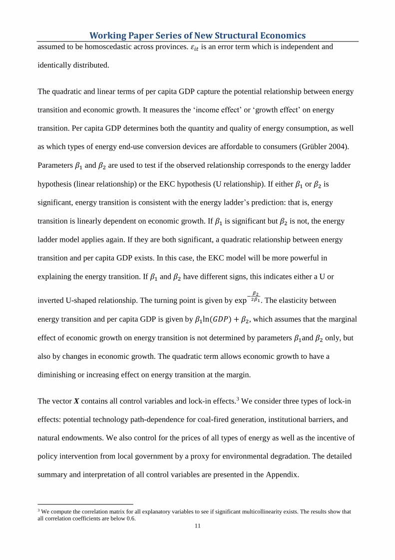
The carbon lock-in theory generally posits that people’s present fuel choices depend on what they

have chosen in the past. In this context, the energy transition is path-dependent. The theory suggests

that the degree of energy transition depends on some exogenous factor such as institution,

technology or infrastructure. Arthur (1989) comments that carbon lock-in occurs when a carbon-

intensive technology is scaled-up. Some studies show that countries with large fossil fuel reserves

tend to change their energy structure slowly -a natural endowment effect (Burke 2013, Burke 2010).

Others argue that energy transition can be locked into several interrelated factors such as the

dominant technology and policy interventions. They regard energy, technology and institution as a

co-evolutionary system (Rio and Unruh 2007). Differing from the energy ladder and EKC, the

carbon lock-in theory postulates that energy transition may be hindered even though per capita GDP

is growing. It is a more pessimistic view of energy transition compared to the other two.

Each of these three theories provides a different perspective on energy transition. To investigate

what pattern China did follow and which theory would explain China’s energy transition well, we

first review stylized facts about China’s energy transition in the next section.

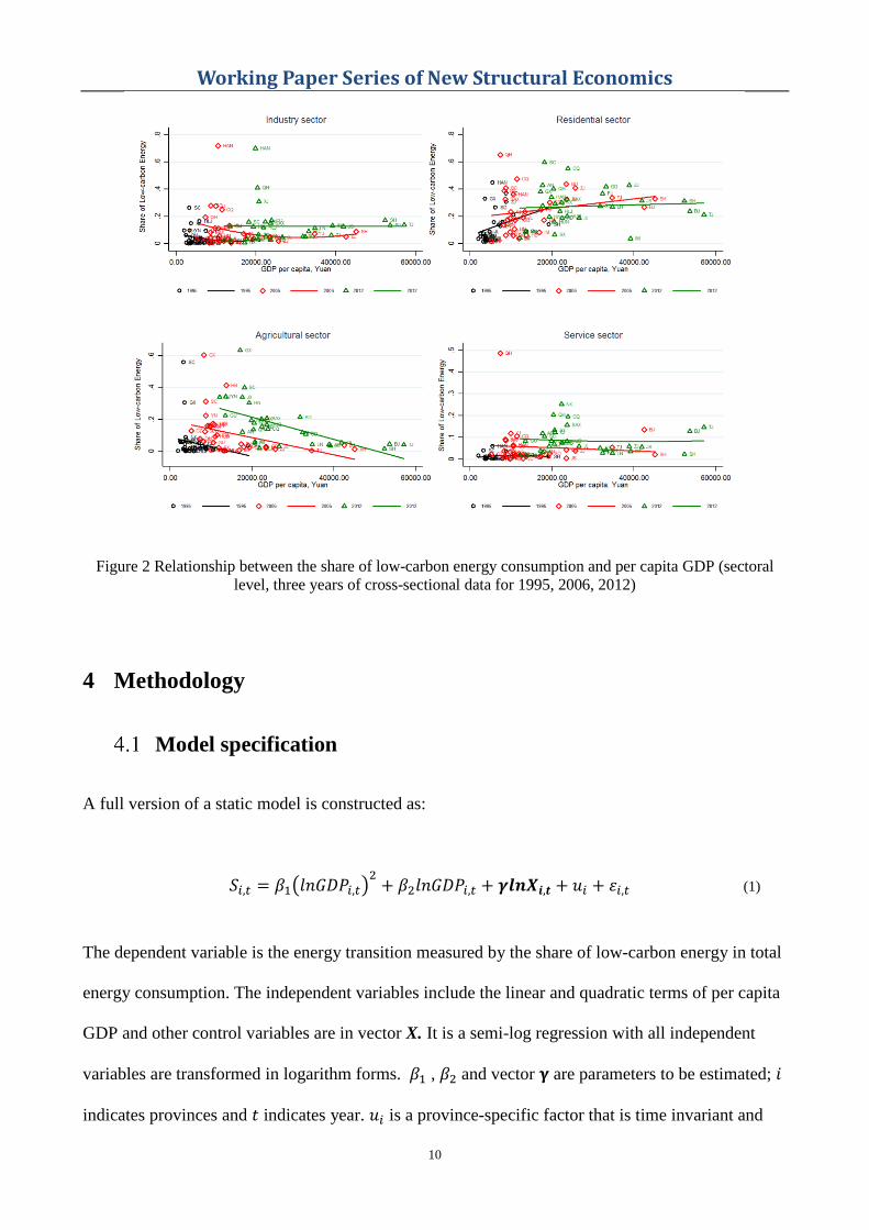
3 Stylized facts

In this paper, we measure China’s energy transition by the share of low-carbon energy in total

energy consumption. The fuel type choice and the calculation process can be seen in the Appendix.

Figure 1 graphs the cross-sectional distribution of energy transition against per capita GDP in 1995,

2006 and 2012. Per capita GDP is measured at the 2010 constant price.2 The level of energy

transition is seen to rise over time. When per capita GDP is below 20,000 Yuan, the transition curve

followed an inverted U curve in 1995 but it changed to a standard U-curve in 2006 when most

provinces achieved a per capita GDP of nearly 20,000 Yuan and moving towards 40,000 Yuan. In

2012, per capita GDP in most provinces was between 20,000 to 40,000 Yuan, with some exceeding

2 We use GDP deflator issued by World Bank http://data.worldbank.org.cn/indicator/NY.GDP.DEFL.ZS, based year is 2010.

http://data.worldbank.org.cn/indicator/NY.GDP.DEFL.ZS


9

40,000 Yuan (Beijing, Tianjin, Shanghai, Jiangsu). The relationship between energy transition and

per capita GDP after 2006 shows an upward linear trend, suggesting that the relationship between

energy transition and economic growth may change at different stages of development.

Figure 1 Relationship between the share of low-carbon energy and GDP per capita (national level, three

years of cross-sectional data for 1995, 2006, 2012)

The sectoral level data are presented in Figure 2. The patterns of the industry sector and service

sector are almost linear and flat with time. It may suggest the energy transition in this sector has no

bearing with per capita GDP. All three curves of the agricultural sector have negative slopes,

suggesting a negative relationship between energy transition and economic growth. In other words,

the agricultural sector tends to consume high-carbon energy rather than low-carbon energy during

economic growth. In the residential sector, the curves are linear and the slops are becoming flattered

over the years; Figure 2 suggest that the causal relationship between energy transition and economic

growth differs across sectors.


10

Figure 2 Relationship between the share of low-carbon energy consumption and per capita GDP (sectoral

level, three years of cross-sectional data for 1995, 2006, 2012)

4 Methodology

Model specification

A full version of a static model is constructed as:

𝑆𝑖,𝑡 = 𝛽1(𝑙𝑛𝐺𝐷𝑃𝑖,𝑡)2

+ 𝛽2𝑙𝑛𝐺𝐷𝑃𝑖,𝑡 + 𝜸𝒍𝒏𝑿𝒊,𝒕 + 𝑢𝑖 + 𝜀𝑖,𝑡

(1)

The dependent variable is the energy transition measured by the share of low-carbon energy in total

energy consumption. The independent variables include the linear and quadratic terms of per capita

GDP and other control variables are in vector X. It is a semi-log regression with all independent

variables are transformed in logarithm forms. 𝛽1 , 𝛽2 and vector 𝛄 are parameters to be estimated; 𝑖

indicates provinces and 𝑡 indicates year. 𝑢𝑖 is a province-specific factor that is time invariant and


11

assumed to be homoscedastic across provinces. 𝜀𝑖𝑡 is an error term which is independent and

identically distributed.

The quadratic and linear terms of per capita GDP capture the potential relationship between energy

transition and economic growth. It measures the ‘income effect’ or ‘growth effect’ on energy

transition. Per capita GDP determines both the quantity and quality of energy consumption, as well

as which types of energy end-use conversion devices are affordable to consumers (Grübler 2004).

Parameters 𝛽1 and 𝛽2 are used to test if the observed relationship corresponds to the energy ladder

hypothesis (linear relationship) or the EKC hypothesis (U relationship). If either 𝛽1 or 𝛽2 is

significant, energy transition is consistent with the energy ladder’s prediction: that is, energy

transition is linearly dependent on economic growth. If 𝛽1 is significant but 𝛽2 is not, the energy

ladder model applies again. If they are both significant, a quadratic relationship between energy

transition and per capita GDP exists. In this case, the EKC model will be more powerful in

explaining the energy transition. If 𝛽1 and 𝛽2 have different signs, this indicates either a U or

inverted U-shaped relationship. The turning point is given by exp−

𝛽22𝛽1. The elasticity between

energy transition and per capita GDP is given by 𝛽1ln (𝐺𝐷𝑃) + 𝛽2, which assumes that the marginal

effect of economic growth on energy transition is not determined by parameters 𝛽1and 𝛽2 only, but

also by changes in economic growth. The quadratic term allows economic growth to have a

diminishing or increasing effect on energy transition at the margin.

The vector X contains all control variables and lock-in effects.3 We consider three types of lock-in

effects: potential technology path-dependence for coal-fired generation, institutional barriers, and

natural endowments. We also control for the prices of all types of energy as well as the incentive of

policy intervention from local government by a proxy for environmental degradation. The detailed

summary and interpretation of all control variables are presented in the Appendix.

3 We compute the correlation matrix for all explanatory variables to see if significant multicollinearity exists. The results show that

all correlation coefficients are below 0.6.


12

The current state of energy transition may depend upon past conditions of itself: persistence,

consumption behavior formation, partial adjustment, and so forth. Therefore, we include the lagged

term of the dependent variable in the dynamic model:

𝑆𝑖,𝑡 = 𝛽0𝑆𝑖,𝑡−1 + 𝛽1(𝑙𝑛𝐺𝐷𝑃𝑖,𝑡)2

+ 𝛽2𝑙𝑛𝐺𝐷𝑃𝑖,𝑡 + 𝜸𝒍𝒏𝑿𝒊,𝒕 + 𝑢𝑖 + 𝜀𝑖,𝑡 (2)

where 𝛽0 is the parameter of the first-lagged dependent variable and the rate of convergence can be

expressed as 1 − 𝛽0, which implies the speed of adjustment. If 𝛽0 = 0, the dependent variable does

not depend on the previous period’s state. If 𝛽0 = 1, there is no dynamic adjustment process

because the energy transition is in the steady state in every period. Given the model dynamics, 𝜸

1−𝛽0

captures the long-run effect of X on energy transition.

Fixed effect

The fixed effect term 𝑢𝑖 in equations (1) and (2) captures all unobservable time-invariant effects

across provinces. The fixed effect can result from typical social norms regarding energy transition

or fuel-consuming patterns within a province. These factors are highly variable across China’s

provinces as there are distinct features of development across provinces. The Hausman test is used

to choose between the fixed effect and the random effect models.4

For robustness and comparison, we also estimate the model using the Fama-MacBeth (FMB) model

and ordinary least squares (OLS). The OLS estimator is biased and inconsistent in the presence of

fixed effects. The Fama–MacBeth two-step procedure (Fama and MacBeth 1973) is implemented in

two steps: first we estimate cross-sectional regression by OLS for every single year; later we

4 Differences within time series and between individuals have long been discussed since Baltagi and Griffin (1984) in literature.

Generally, Panel data involves two types of variation: the differences between provinces (between variations) and the differences

over time within provinces (within variation). Firstly, we proceed to the Ordinary Least-Squares (OLS) estimator, fixed-effect (FE)

estimator and random-effect (RE) estimator for model choice. The rejection from the likelihood ratio test indicates FE is superior to

OLS. Breusch and Pagan Lagrangian multiplier test shows that RE estimator are better than OLS too. We finally adopt FE on basis of

rejection of Hausman test between FE and RE. In this case, RE model is biased.


13

average coefficient estimates from the first step using Zellner's seemingly unrelated regression

(SUR) estimation. This procedure allows us to include the over-year variation in coefficients. For T

→∞, these averages will provide consistent estimators for the population. The standard errors are

computed from the sample standard deviations of estimated coefficients, treating them as

independent drawings from a common pool. The standard error calculation allows for arbitrary

cross-sectional correlation and heteroscedasticity in residuals. The Fama–MacBeth procedure can

provide a heteroscedasticity-consistent estimation in the absence of serial correlation. However,

given the existence of a serial correlation, in this case, we adjust it via Newey and West (1987)

standard error estimates with a lag length of two periods.

Generalized method of moments

The dynamic model might give rise to ‘dynamic panel bias’ because the lagged dependent variable

may be positively correlated with fixed effect so that the OLS estimator is inconsistent and

overestimates the true autoregressive coefficient 𝛽0 (Nickell 1981). Given that the lagged term

exists, the FE is inconsistent because the within transformed lagged dependent variable is correlated

with the within transformed error. Given the finite time period T and provinces N, FE model

underestimates the true autoregressive coefficient 𝛽0 (Verbeek 2012, 396).

To deal with this potential endogeneity problem, we use the generalized method of moments

(GMM) to estimate the dynamic model. This method is particularly suitable for a dynamic model

with a few years and large groups. Anderson and Hsiao (1981) propose difference GMM to remove

fixed effect by first-difference transforming data as follow:

∆𝑆𝑖,𝑡 = 𝛼∆𝑆𝑖,𝑡−1 + 𝛽1∆(𝑙𝑛𝐺𝐷𝑃𝑖,𝑡)2 + 𝛽2∆𝑙𝑛𝐺𝐷𝑃𝑖,𝑡 + 𝜸∆𝒍𝒏𝑿𝒊,𝒕 + ∆𝜀𝑖,𝑡 (3)

GMM does not require that the error term is independent and identically distributed over provinces

and years, but the consistency of estimators assumes that 𝜀𝑖,𝑡 does not exhibit autocorrelation.


14

Difference GMM still has potential endogeneity problems, since the lagged dependent variable is

still potentially endogenous with the changes of disturbance by way of 𝑆𝑖,𝑡−1 in ∆𝑆𝑖,𝑡−1 is correlated

with 𝜀𝑖,𝑡−1 in ∆𝜀𝑖,𝑡. In addition, some predetermined explanatory variables may not be strictly

exogenous as they are correlated with 𝜀𝑖,𝑡−1. Therefore, we instrument ∆𝑆𝑖,𝑡−1 by 𝑆𝑖,𝑡−2 or further

lagged terms.

Arellano and Bond (1991) note that difference GMM does not employ all the necessary moment

conditions. Thus, if some independent variables are not strictly exogenous but are predetermined,

difference GMM does not always guarantee efficiency estimates by applying instrument variables.

More important, Blundell and Bond (1998) point out that the first difference GMM may suffer from

finite sample biases, particularly in a situation where the dependent variable shows high persistence;

that is, 𝛼 is close to one. In other words, past levels convey little information about future changes.

In such situations, the instruments are weak because they provide very little information on the

parameters of interest. Blundell and Bond (1998) introduce the system GMM method that uses

moment conditions based on both levels and first-differences equations. The significant advantage

of system GMM is that it avoids losing information by differencing the fixed effect. In this paper,

we employ both difference and system GMM methods for our dynamic model estimations.

5 Variables and data

The detailed data source and the summary of variables are presented in the Appendix.

Provinces with large natural endowments of some energy resources are usually reluctant to change

consumption habits as this abundant energy is readily available and has low transport costs,

especially given the well-developed rails and waterways in China. Such effects have been observed

in several cross-country studies (Burke 2010, Burke 2011, 2012, 2013). In modeling, we control for

three main types of energy resource endowment: coal, oil and natural gas, to test if energy transition

could be locked in by resource abundance. A suitable proxy is needed to measure the amount of


15

natural endowment. Some candidates have been suggested in the literature: for instance, some

economists are using export energy data (Sachs and Warner 1995, Davis 1995) while others use

resource rent data (Stijns 2006). We adopt Brunnschweiler’s (2008) measurement of per capita

production as an indicator of the natural endowment.

Energy transition may be locked in by fossil technologies increasing return to scale (Unruh 2000).

Large numbers of coal-powered plants may lock a province into using coal for its electricity

production. To negate the scale effect of the economy, we use per capita coal-fired power

generation capacity (installed) as a proxy to investigate potential technology lock-in.

Urbanization can be regarded as an institutional change during the transition from agrarianism to

industrialization. A feature of China’s reform and rapid growth during the past decades is internal

rural-urban migration, which is partially driven by institutional arrangements such as the Hukou

system5 reform, the social insurance system, urban infrastructure investment, and like human rights

related to equality. Herrerias, Aller, and Ordonez (2017) find that the energy mix in urban areas

changed when electricity replaced coal, and they consider that urbanization accounts for this,

especially in the areas of Hukou reform and the New Urbanisation policy. We use the number of

people living in urban areas to indicate this major institutional change: the more people in an urban

area, the more sophisticated society becomes and the better is the quality of its institutions. Urban

population is measured by the number of people living in towns and city. We use actual residential

population rather than registered population.

We control policy effect as a proxy of the lagged term of yearly changes of sulfur dioxide (SO2)

emission as it can measure the tightness of the environmental policy. Sulfur dioxide is one of the

main pollutants from the use of coal and oil. It is a major indicator of pollution and is strictly

5 A Hukou is a record in a government system of household registration required by law in mainland China and Taiwan, and

determines where citizens can live. Because of its entrenchment of social strata, especially between rural and urban residency status,

the hukou system is often regarded as a form of caste system.


16

monitored by the Ministry of Environmental Protection and other authorities who use it to assess

the performance of the environmental governance of local governments. We use the changes in the

logarithm of sulfur dioxide between every adjacent two years to measure the slackness of

environmental policy. The underlying assumption is that if an increase in SO2 emissions were high

in last year, the local government would come under more pressure to adopt policy actions on

energy transition this year. The policy effectiveness is based on the performance of SO2 emissions.

6 Results

The consistency of the fixed effect estimator will not guarantee efficiency all the time if the error

term is heteroscedastic or displays autocorrelation or cross-sectional dependence. We adopt a

modified Wald statistic following Greene (2012, 338) to test for potential province-wise

heteroscedasticity in the residuals of the national level model as well as sectoral level models. The

null hypothesis is that there is no heteroscedasticity in the model. Tests for autocorrelation,

heteroscedasticity and cross-sectional independence and unit roots are reported in the Appendix.

The model residuals may also suffer from autocorrelation; thus estimated parameters will be

inefficient but still unbiased. The Wooldridge test is used to test for autocorrelation. The null

hypothesis is no series correlation and we reject it at the 5% level in the sectoral level models

except for the national level model. Thus, all sectoral level regression performs first-order serial

correlation. Under such circumstances, FE is still consistent, but inefficient, and standard error

estimates are biased.

We suspect the model residuals are correlated within or between provinces. The Wald test on the

FE model is rejected, indicating province-wise heteroscedasticity exists. We are also concerned that

provinces may suffer from the problem of spatial dependence (neighborhood effect), which may

occur if the social norms or psychological behavior patterns are influenced by neighboring

provinces. In theory, Hoechle (2007) suggests this cross-sectional correlation may result from the


17

explanatory variables and disturbance terms containing three components: an individual specific

long-run mean, an autocorrelated common factor, and an idiosyncratic forcing term. We conduct the

Pesaran test to check this. The null hypothesis is that the residuals are cross-sectionally

uncorrelated. The Pesaran test shows that the residuals in the agricultural model present cross-

sectional dependence, which implies energy transition could be spatially correlated in the

agricultural sector.

To ensure valid inferences, we adopt the Driscoll–Kraay FE estimator (Hoechle 2007) for the

agricultural model. With this estimator, we can relax assumptions by allowing residuals to be

correlated both within groups and between groups, to take account of spatial correlation in the

model. The Driscoll–Kraay estimator also adjusts the standard error estimates by sequencing cross-

sectional averages of the moment conditions, which guarantees consistency and independence of

cross-sectional dimension N. We adopt Rogers standard errors (clustered standard errors) to

compute standard errors for the industry, service and residential sector models (Cameron and Miller

2015). Rogers standard errors allow for residuals that are heteroscedastic and correlated within

groups but not between groups.

We estimate the fixed effect model for the whole period and the subperiod after 2005, to investigate

if the significance level of some variables changed after 2005 when the national energy transition

initiative was launched.6

Table 1 and Table 2 are estimations of the national level static and dynamic models, respectively.

Sectoral transition estimations are reported in Table 3 to Table 6, for the industry, agricultural,

service and residential sectors separately.

6 China’s government has made a commitment that by 2020 non-fossil energy will account for 15 percent of total primary energy

consumption, and that CO2 emission per GDP will be 40–45 percent lower than that in 2005. This is stipulated in the twelfth Five-

Year Plan (2011–2015) for National Economic and Social Development, and calls for a significant energy transition. Meanwhile,

China’s economic growth will decouple from energy consumption to some extent. The initial set of China’s energy pricing reform

started in 2005, with a focus of establishing a market-oriented market to reduce energy price differences in different regions (Guo et

al. 2015). A target to improve 20 percent energy efficiency by 2012 was also set in 2005. For the sake of testing this policy effect,

we run the subsample before and after 2005 separately.


18

National level results

At the national level, a significant U curve relationship is found between energy transition and per

capita GDP as can be seen in Table 1. Except for the subperiod before 2005, all the other models’

coefficients for per capita GDP quadratic terms are significantly positive and the coefficients for per

capita GDP linear terms are significantly negative. The energy transition pattern shifted from 2005

when the National Energy Transition Initiatives launched. However, the turning points are different

across the models. Given that the Fama–MacBeth and OLS are biased estimations, the FE models

are more robustness and they suggest that the turning point is around 15,000 – 16,000 Yuan.

The FE models for the two subperiods before and after 2005, shown in columns (4) and (5), provide

different significance levels. We find the natural gas endowment effect changes from insignificant

to positively significant. After 2005, a 1% increase in natural gas production will increase the low-

carbon energy share by 0.007 percent point. It could be a result of the natural gas stimulation policy.

The price effects became more significant after 2005 too. A 1% increase in the steam coal price will

result in 0.093 percent point increase in the low-carbon energy share; 1% increase in residential

electricity price will increase the low-carbon energy share by 0.102 percent point; 1% increase in

diesel price will increase low-carbon energy share by 0.079 percent point, ceteris paribus. These

results indicate that price fluctuation is effective to promote energy transition and the deregulation

policy reform that decentralizes the energy market would be valid to assist China to get into a low-

carbon and sustainable development trajectory (Guo et al. 2015).


19

Table 1 Results for the national level static model

Model (1) (2) (3) (4) (5)

Variable FMB OLS_Pooled FE FE_before2005 FE_post2005

ln(GDP)2 0.024** 0.018** 0.044*** -0.075** 0.084***

(0.032) (0.030) (0.001) (0.033) (0.000)

ln(GDP) -0.417* -0.336** -0.847*** 1.454** -1.634***

(0.066) (0.042) (0.001) (0.026) (0.000)

ln(coalgen) -0.064*** -0.052*** 0.041** -0.004 0.015

(0.000) (0.000) (0.029) (0.894) (0.568)

ln(urban) -0.047*** -0.064*** 0.030 0.009 -0.043

(0.001) (0.000) (0.147) (0.791) (0.689)

ln(gas) 0.021*** 0.019*** 0.010*** 0.004 0.007*

(0.000) (0.000) (0.006) (0.509) (0.055)

ln(oil) -0.002 -0.003** -0.001 -0.004 0.000

(0.280) (0.027) (0.863) (0.545) (0.964)

ln(coal) -0.020*** -0.022*** -0.006 -0.021 0.000

(0.000) (0.000) (0.397) (0.383) (0.995)

ln(𝑃𝑏𝑟𝑖𝑞𝑢𝑒𝑡) -0.031* -0.009 -0.014 -0.044* 0.000

(0.067) (0.379) (0.235) (0.085) (0.996)

ln(𝑃𝑠𝑡𝑒𝑎𝑚𝑐𝑜𝑎𝑙) 0.007 0.002 0.019 -0.030 0.093***

(0.457) (0.846) (0.321) (0.418) (0.000)

ln(𝑃𝑒𝑙𝑒𝑐𝑖𝑛𝑑) -0.061 -0.039 0.032 0.044 0.040

(0.138) (0.147) (0.317) (0.543) (0.428)

ln(𝑃𝑒𝑙𝑒𝑐𝑟𝑒) -0.037 0.053* 0.027 -0.050 0.102***

(0.359) (0.091) (0.534) (0.486) (0.010)

ln(𝑃𝑒𝑙𝑒𝑐𝑎𝑔) -0.059 -0.006 -0.021 0.036 -0.001

(0.128) (0.654) (0.173) (0.818) (0.921)

ln(𝑃𝑒𝑙𝑒𝑐𝑠𝑒𝑟𝑣) -0.070 -0.102*** 0.079** 0.049 0.052

(0.133) (0.002) (0.038) (0.795) (0.195)

ln(𝑃𝑝𝑒𝑡𝑟𝑜) 0.699* 0.233*** 0.067 0.183 -0.144

(0.071) (0.009) (0.527) (0.367) (0.242)

ln(𝑃𝑑𝑖𝑒𝑠𝑒𝑙) -0.164*** -0.040 0.037 -0.200* 0.079*

(0.002) (0.151) (0.368) (0.085) (0.092)

ln(𝑃𝑔𝑎𝑠𝑖𝑛𝑑) -0.031 -0.041** -0.031 -0.020 -0.043

(0.487) (0.022) (0.107) (0.433) (0.234)

ln(𝑃𝑔𝑎𝑠𝑟𝑒) -0.057 -0.059** 0.013 0.039 0.069

(0.266) (0.021) (0.690) (0.464) (0.520)

dln(SO2) 0.055 0.042 0.023 0.004 0.023

(0.486) (0.165) (0.346) (0.854) (0.388)

constant -2.426 0.747 2.837** -6.557** 8.487***

(0.511) (0.527) (0.045) (0.041) (0.000)

N 330 330 330 120 210

R2 0.919 0.814 0.404 0.415 0.309

Turning point 6062.519 9534.2395 15356.216 16285.513 16146.216 Note: p-values in parentheses * p < 0.1, ** p < 0.05, *** p < 0.01. year dummies are eliminated to save space.

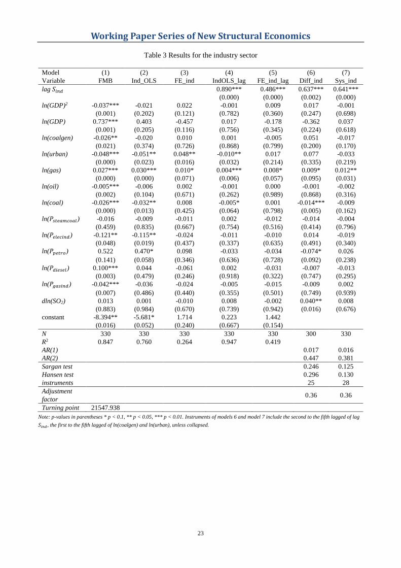
Focusing on the FE model of the whole period (model 3), we find that the coefficient of natural gas

production to energy transition is significantly positive (0.010), slightly higher than in the post-2005

model (0.007). It implies a stronger effect of natural gas resource endowment in the long run. The

coefficient of coal-fired electricity generation capacity is significantly positive (0.041), suggesting

that a 1% increase in coal-fired power generation would increase energy transition by 0.041 percent

point, rather than hindering the transition. The seemingly counterintuitive facts can be explained by


20

reviewing the historical stages of development. At early stages of development, when the

households directly burn coal for heating or cooking, the burning coal and electricity would be

substitutes. Hence, generating electricity, even from coal, could significantly reduce direct coal

consumption in a less developed society.

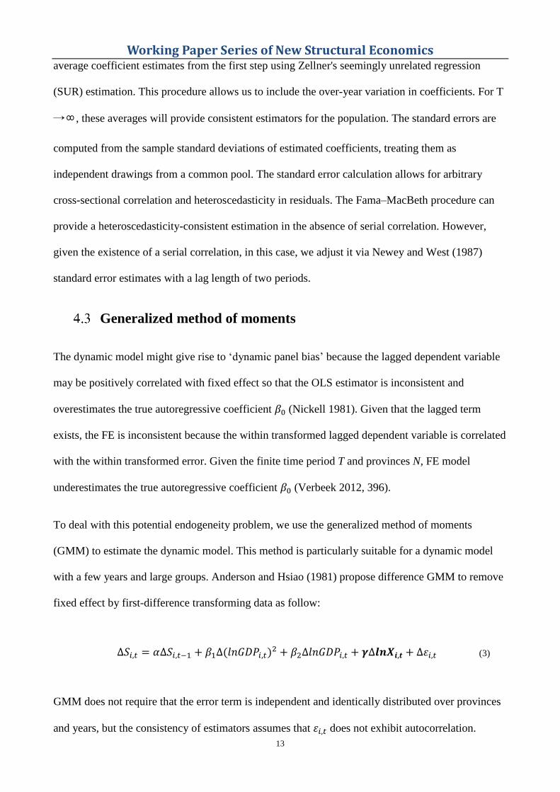
In Table 2, we report the national level dynamic model results. Columns (1) to (4) are the OLS, FE,

difference GMM and system GMM models, respectively.7 All the models suggest a U-curve

relationship between energy transition and per capita GDP. The difference and system GMM model

suggest that the turning points are about 17,263 or 15,345 Yuan, based on the 2010 constant price.

The Sargan and Hansen’s tests show that both the difference and system GMM models are

appropriate for the selected instruments. As the system GMM model contains more information on

the level equation for inference, we are prone to adopt the turning point suggesting by the system

GMM model (15,345.213 Yuan). This number is very close to the turning point suggested by the

static FE model in Table 1 (15,356.216 Yuan).

Apparently, from the system GMM model, the energy transition performs some pattern of self-

persistence with the coefficient of 0.267 and the speed of adjustment is 0.733. We can also observe

a significant natural resource endowment effect and price effect. In the long-run,8 a 1% increase in

the natural gas production will increase low-carbon energy share by 0.022 percent point; a 1%

increase in petroleum price will increase low-carbon energy share by 0.188 percent point, ceteris

paribus. On the contrary, a long-run effect of 1% increase in industrial electricity price or industry

natural gas price will significantly decrease energy transition by 0.119 and 0.111 percent point,

respectively. Apart from these, we find the national energy mix would be locked into the coal-

electricity power generation capacity by the long-run coefficient of 0.022 percent point.

7 As discussed earlier, OLS tends to overestimate the parameter of the lagged term while FE tends to underestimate it. The true

coefficient should lie somewhere between them. The estimated coefficients of the lagged transition index in models (3) and (4) lies

between those of the OLS and the fixed effect models indicating that the results of the GMM estimation are reliable. 8 The long-run coefficient of dynamic GMM model is given by γ/(1 − 𝛽0), as illustrated in Equation (3).


21

Table 2 Results for the national level dynamic model

Model (1) (2) (3) (4)

Variable OLS_lag FE_lag Diff_GMM Sys_GMM

lag S 0.657*** 0.224*** 0.379 0.267*

(0.000) (0.000) (0.371) (0.073)

ln(GDP)2 0.015** 0.041*** 0.045* 0.016***

(0.016) (0.000) (0.052) (0.005)

ln(GDP) -0.282** -0.781*** -0.868* -0.314***

(0.018) (0.000) (0.056) (0.005)

ln(coalgen) -0.014** 0.033** 0.069 -0.016

(0.026) (0.036) (0.197) (0.377)

ln(urban) -0.023*** 0.019 0.071 0.015

(0.001) (0.287) (0.755) (0.459)

ln(gas) 0.007*** 0.008*** 0.011** 0.016***

(0.000) (0.008) (0.029) (0.001)

ln(oil) -0.001 0.000 0.008 -0.002

(0.157) (0.956) (0.116) (0.552)

ln(coal) -0.009*** -0.006 -0.005 -0.027***

(0.000) (0.350) (0.746) (0.002)

ln(𝑃𝑏𝑟𝑖𝑞𝑢𝑒𝑡) -0.006 -0.012 -0.045** -0.027*

(0.501) (0.223) (0.044) (0.068)

ln(𝑃𝑠𝑡𝑒𝑎𝑚𝑐𝑜𝑎𝑙) 0.005 0.025 0.052** 0.006

(0.595) (0.170) (0.031) (0.757)

ln(𝑃𝑒𝑙𝑒𝑐𝑖𝑛𝑑) -0.021 0.025 0.043 -0.087**

(0.232) (0.373) (0.542) (0.011)

ln(𝑃𝑒𝑙𝑒𝑐𝑟𝑒) 0.025 0.022 0.002 -0.046

(0.249) (0.552) (0.977) (0.240)

ln(𝑃𝑒𝑙𝑒𝑐𝑎𝑔) -0.000 -0.013 -0.024 -0.026

(0.964) (0.347) (0.515) (0.309)

ln(𝑃𝑒𝑙𝑒𝑐𝑠𝑒𝑟𝑣) -0.033 0.062* 0.091 -0.090

(0.173) (0.069) (0.515) (0.124)

ln(𝑃𝑝𝑒𝑡𝑟𝑜) 0.015 0.030 -0.005 0.138***

(0.850) (0.738) (0.952) (0.000)

ln(𝑃𝑑𝑖𝑒𝑠𝑒𝑙) -0.011 0.033 0.000 0.038

(0.625) (0.288) (0.999) (0.131)

ln(𝑃𝑔𝑎𝑠𝑖𝑛𝑑) -0.024* -0.027 -0.060 -0.081***

(0.059) (0.116) (0.183) (0.001)

ln(𝑃𝑔𝑎𝑠𝑟𝑒) -0.014 0.025 0.059 -0.005

(0.442) (0.364) (0.440) (0.885)

dln(SO2) 0.005 0.011 0.014 0.009

(0.789) (0.613) (0.760) (0.688)

constant 1.544 2.897**

(0.116) (0.013)

N 330 330 300 330

R2 0.894 0.436

AR(1)1 0.097 0.003

AR(2)2 0.737 0.753

Sargan test 0.369 0.032

Hansen test 0.268 0.340

Instruments 23 26

Adjustment factor 0.621 0.733

Turning point 17263.092 15345.213 Note: p-values in parentheses * p < 0.1, ** p < 0.05, *** p < 0.01; 1,2. Arellano–Bond test for AR(1) and AR(2)

Instruments for model 3 include the second lagged to fourth lagged of lag S and the first and second lagged of ln(urban) and ln(coalgen), unless

collapsed. Instruments for model 4 include the first to third lagged of lag S and the first and second lagged of ln(urban) and ln(coalgen), unless collapsed.


22

Industry sector results

Table 3 reports results for the industry sector. Columns (1) to (3) are for the static models and

columns (4) to (7) are for the dynamic models. We can see that except for the FMB in column (1),

the quadratic and linear terms of per capita GDP are all insignificant. The lagged terms of energy

transition are all highly significant and the magnitudes are relatively high. It suggests a significant

self-perpetuating process of energy transition which is independent of GDP per capita in the

industry sector. In this case, FMB estimates are inappropriate as errors are likely to be as severely

correlated over time as across provinces and GMM can be used to correct the estimates (Cochrane

2001). According to the difference and system GMM model in column (6) and (7), energy transition

can be stimulated by 0.009 and 0.012 percent point respectively if the natural gas abundance

increased by 1%, which indicates a significant natural resource endowment effect. We can also find

in the difference GMM model that the energy transition may be locked in by coal reserve

endowment at the margin of -0.014. That is, a 1% increase in coal production will decrease energy

transition by 0.04 percent point in the long run. The price effect of petroleum is significant by the

margin of -0.074. That is, a 1% increase in petroleum price will decrease low-carbon energy share

by 0.2 in the long run. It implies that petroleum price increase would not result in substitution

between oil and natural gas; on the contrary, it reversely shifts the energy consumption to coal. It

could because coal is easier to access than natural gas in terms of availability and price. We also

observe a significant policy effect by the difference GMM model. If the government implements

stricter environmental regulations on the factories, it will increase energy transition by 0.11 percent

point in the long run.

In the static model, we find that urbanization and natural gas endowments will significantly increase

energy transition by 0.048 and 0.01 percent points respectively if they increase 1% at the margin.


23

Table 3 Results for the industry sector

Model (1) (2) (3) (4) (5) (6) (7)

Variable FMB Ind_OLS FE_ind IndOLS_lag FE_ind_lag Diff_ind Sys_ind

lag 𝑆𝑖𝑛𝑑 0.890*** 0.486*** 0.637*** 0.641***

(0.000) (0.000) (0.002) (0.000)

ln(GDP)2 -0.037*** -0.021 0.022 -0.001 0.009 0.017 -0.001

(0.001) (0.202) (0.121) (0.782) (0.360) (0.247) (0.698)

ln(GDP) 0.737*** 0.403 -0.457 0.017 -0.178 -0.362 0.037

(0.001) (0.205) (0.116) (0.756) (0.345) (0.224) (0.618)

ln(coalgen) -0.026** -0.020 0.010 0.001 -0.005 0.051 -0.017

(0.021) (0.374) (0.726) (0.868) (0.799) (0.200) (0.170)

ln(urban) -0.048*** -0.051** 0.048** -0.010** 0.017 0.077 -0.033

(0.000) (0.023) (0.016) (0.032) (0.214) (0.335) (0.219)

ln(gas) 0.027*** 0.030*** 0.010* 0.004*** 0.008* 0.009* 0.012**

(0.000) (0.000) (0.071) (0.006) (0.057) (0.095) (0.031)

ln(oil) -0.005*** -0.006 0.002 -0.001 0.000 -0.001 -0.002

(0.002) (0.104) (0.671) (0.262) (0.989) (0.868) (0.316)

ln(coal) -0.026*** -0.032** 0.008 -0.005* 0.001 -0.014*** -0.009

(0.000) (0.013) (0.425) (0.064) (0.798) (0.005) (0.162)

ln(𝑃𝑠𝑡𝑒𝑎𝑚𝑐𝑜𝑎𝑙) -0.016 -0.009 -0.011 0.002 -0.012 -0.014 -0.004

(0.459) (0.835) (0.667) (0.754) (0.516) (0.414) (0.796)

ln(𝑃𝑒𝑙𝑒𝑐𝑖𝑛𝑑) -0.121** -0.115** -0.024 -0.011 -0.010 0.014 -0.019

(0.048) (0.019) (0.437) (0.337) (0.635) (0.491) (0.340)

ln(𝑃𝑝𝑒𝑡𝑟𝑜) 0.522 0.470* 0.098 -0.033 -0.034 -0.074* 0.026

(0.141) (0.058) (0.346) (0.636) (0.728) (0.092) (0.238)

ln(𝑃𝑑𝑖𝑒𝑠𝑒𝑙) 0.100*** 0.044 -0.061 0.002 -0.031 -0.007 -0.013

(0.003) (0.479) (0.246) (0.918) (0.322) (0.747) (0.295)

ln(𝑃𝑔𝑎𝑠𝑖𝑛𝑑) -0.042*** -0.036 -0.024 -0.005 -0.015 -0.009 0.002

(0.007) (0.486) (0.440) (0.355) (0.501) (0.749) (0.939)

dln(SO2) 0.013 0.001 -0.010 0.008 -0.002 0.040** 0.008

(0.883) (0.984) (0.670) (0.739) (0.942) (0.016) (0.676)

constant -8.394** -5.681* 1.714 0.223 1.442

(0.016) (0.052) (0.240) (0.667) (0.154)

N 330 330 330 330 330 300 330

R2 0.847 0.760 0.264 0.947 0.419

AR(1) 0.017 0.016

AR(2) 0.447 0.381



instruments 25 28

Adjustment

factor 0.36 0.36

Turning point 21547.938

Note: p-values in parentheses * p < 0.1, ** p < 0.05, *** p < 0.01. Instruments of models 6 and model 7 include the second to the fifth lagged of lag

𝑆𝑖𝑛𝑑, the first to the fifth lagged of ln(coalgen) and ln(urban), unless collapsed.


24

Agricultural sector results

Table 4 reports the agricultural sector results. In the dynamic model, we find a significant self-

perpetuating process of energy transition which is similar to the results of the industry sector. The

coefficient of the lagged term of the energy transition is 0.837, and all the other variables are

insignificant. In the static model, we find an inverted U-curve relationship between energy

transition and per capita GDP in the static FE model in column (3).

In contrast, a U-curve relationship is found in the FMB model. We advocate FE result here as, given

the presence of heterogeneity of provinces, the standard error estimate from FMB would be too

small to be correct in terms of significance level (Petersen 2008). The installed coal-fired electricity

generation would increase the energy transition in agriculture by a margin of 0.008 percent point,

which could be a result of shifting burning coal to electricity in the rural area. An increase in

petroleum and diesel price will decrease the energy transition instead of increasing low-carbon

energy consumption such as natural gas, which indicates a potentially reverse energy transition to

coal. It could happen in the use of some agricultural and aquaculture facilities, such as greenhouses,

sheds, temperature regulation, incubators or in the production of fertilizer. When the oil products

become expensive, farmers may use coal to substitute oil consumption as other low-carbon energies

are more expensive, or they cannot access the network of natural gas or electricity.

The turning point of FE is 14,952 Yuan, which is very close to the turning points found by the

national level model though the patterns are opposite. Whether the energy transition in the

agricultural sector is inverted U relationship regarding per capita GDP or it is a solely self-

perpetuating phenomenon is still under debate in the literature. For example, Démurger and

Fournier (2007) argue that fuelwood in rural areas is a kind of ‘inferior good’ and will decrease as

per capita income increases, with the increasing opportunity cost of collecting fuelwood for the

wealthier families. On the other hand, Shi, Heerink, and Qu (2009) use a CGE model to find that


25

fuelwood is a normal good in rural Beijing and will increase as income increases. Overall, the

energy transition in the agricultural sector is more complex.

Table 4 Results for the agricultural sector

Model (1) (2) (3) (4) (5) (6) (7)

Variable FMB OLS FE OLS_lag FE_lag Diff_GMM Sys_GMM

lag 𝑆𝑎𝑔 0.921*** 0.673*** 0.809*** 0.837***

(0.000) (0.000) (0.000) (0.000)

ln(GDP)2 0.053*** -0.022 -0.034*** 0.004 -0.002 0.011 -0.004

(0.003) (0.134) (0.000) (0.238) (0.790) (0.531) (0.338)

ln(GDP) -1.169*** 0.333 0.652*** -0.089 0.057 -0.179 0.041

(0.002) (0.247) (0.000) (0.152) (0.733) (0.596) (0.540)

ln(coalgen) -0.071*** -

0.066***

0.013 0.000 0.019 0.064 0.025

(0.001) (0.004) (0.134) (0.976) (0.118) (0.398) (0.303)

ln(gas) 0.033** 0.008 0.010 0.001 0.005 -0.095 -0.016

(0.020) (0.681) (0.546) (0.540) (0.738) (0.530) (0.477)

ln(oil) -0.006*** -0.007 -0.008 -0.001 -0.005 -0.008 -0.003

(0.006) (0.320) (0.156) (0.279) (0.303) (0.257) (0.378)

ln(coal) -0.020*** -0.020** 0.008** -0.002*** -0.000 -0.004 -0.004

(0.000) (0.014) (0.012) (0.004) (0.969) (0.204) (0.350)

ln(𝑃𝑠𝑡𝑒𝑎𝑚𝑐𝑜𝑎𝑙) -0.003 -0.001 -0.002 0.000 -0.001 0.004 0.001

(0.551) (0.882) (0.687) (0.800) (0.789) (0.779) (0.887)

ln(𝑃𝑏𝑟𝑖𝑞𝑢𝑒𝑡) 0.090*** 0.093** 0.042** 0.014* 0.008 -0.007 0.037

(0.000) (0.030) (0.019) (0.055) (0.633) (0.856) (0.144)

ln(𝑃𝑒𝑙𝑒𝑐𝑎𝑔) -0.105*** -0.065 0.006 -0.010 -0.003 -0.024 -0.015

(0.002) (0.179) (0.779) (0.102) (0.863) (0.245) (0.426)

ln(𝑃𝑝𝑒𝑡𝑟𝑜) 0.017 -0.001 -0.042** 0.008 -0.015 0.017 0.030

(0.566) (0.989) (0.031) (0.193) (0.173) (0.793) (0.276)

ln(𝑃𝑑𝑖𝑒𝑠𝑒𝑙) -0.364*** -

0.265***

-0.025* -0.024 -0.046 0.024 -0.007

(0.006) (0.007) (0.099) (0.186) (0.175) (0.377) (0.740)

dln(SO2) -0.142** -0.116* -0.030 -0.008 0.007 -0.008 -0.021

(0.016) (0.061) (0.198) (0.614) (0.660) (0.684) (0.288)

constant 9.511*** 1.336 -3.144*** 0.719* -0.068

(0.001) (0.457) (0.001) (0.050) (0.943)

N 330 330 330 330 330 300 330

R2 0.712 0.617 0.955 0.693

AR(1) 0.013 0.006

AR(2) 0.953 0.778



instruments 20 23

Adjustment

factor

0.19 0.16

Turning point 14952.158

Note: p-values in parentheses * p < 0.1, ** p < 0.05, *** p < 0.01. 1,2. Arellano-Bond test for AR(1) and AR(2). Year dummies are eliminated to

save space. Instruments of model 6 and 7 include the fourth to the sixed lagged lag 𝑆𝑎𝑔, the fifth to the seventh lagged of ln(coalgen) and ln(urban),

unless collapsed.


26

Service sector results

Table 5 reports the results for the service sector. There is no significant relationship found between

energy transition and per capita GDP across all the models except for the FMB model, which

suggests the energy transition of the service sector is independent of per capita GDP. It is consistent

with the stylized facts presented in Figure 2. It could be because the scale of the service sector is too

small to be observed. The lagged terms of energy transition are significant in all dynamic models,

meaning there is a significant self-evolution of energy transition in the service sector.

Table 5 Results for the service sector Model (1) (2) (3) (4) (5) (6) (7)


lag 𝑆𝑠𝑒𝑟𝑣 0.846*** 0.731*** 0.779*** 0.817***

(0.000) (0.000) (0.000) (0.000)

ln(GDP)2 0.027* 0.013 0.007 0.001 0.005 -0.000 0.003

(0.057) (0.243) (0.470) (0.669) (0.398) (0.977) (0.416)

ln(GDP) -0.504* -0.262 -0.079 -0.026 -0.054 0.003 -0.067

(0.068) (0.245) (0.658) (0.671) (0.561) (0.989) (0.439)

ln(urban) -0.026*** -0.030* -0.029 -0.003* 0.008 0.109 0.010

(0.005) (0.051) (0.197) (0.100) (0.591) (0.647) (0.707)

ln(gas) 0.007** 0.007 -0.001 0.000 -0.002 -0.002 0.001

(0.022) (0.144) (0.810) (0.651) (0.525) (0.542) (0.789)

ln(oil) 0.003** 0.003 0.002 0.001** 0.000 0.002 0.001

(0.023) (0.155) (0.487) (0.020) (0.676) (0.433) (0.353)

ln(coal) -0.009*** -0.006 -0.001 -0.001 -0.003 0.007 -0.003

(0.001) (0.233) (0.894) (0.375) (0.589) (0.504) (0.596)

ln(𝑃𝑠𝑡𝑒𝑎𝑚𝑐𝑜𝑎𝑙) 0.024* 0.015 0.019 -0.000 0.016 -0.003 -0.004

(0.073) (0.595) (0.386) (0.963) (0.230) (0.824) (0.680)

ln(𝑃𝑏𝑟𝑖𝑞𝑢𝑒𝑡) 0.016*** 0.021 -0.019 0.001 -0.007 -0.007 -0.006

(0.006) (0.118) (0.405) (0.893) (0.455) (0.612) (0.564)

ln(𝑃𝑒𝑙𝑒𝑐𝑠𝑒𝑟𝑣) 0.005 0.005 0.107 -0.010 -0.006 -0.061 -0.030

(0.847) (0.898) (0.221) (0.345) (0.798) (0.217) (0.553)

ln(𝑃𝑝𝑒𝑡𝑟𝑜) -0.117 -0.052 0.150 0.036 -0.000 -0.013 0.032

(0.578) (0.743) (0.189) (0.194) (0.989) (0.835) (0.206)

ln(𝑃𝑑𝑖𝑒𝑠𝑒𝑙) -0.070 -0.072 -0.058 -0.023 0.018 0.024 0.005

(0.139) (0.148) (0.636) (0.178) (0.224) (0.463) (0.716)

ln(𝑃𝑔𝑎𝑠𝑖𝑛𝑑) -0.079*** -0.064** -0.039 -0.015* -0.009 0.015 -0.011

(0.000) (0.040) (0.342) (0.057) (0.630) (0.473) (0.380)

constant 3.982 2.384 -0.361 0.054 -0.120

(0.141) (0.276) (0.707) (0.876) (0.760)

N 368 368 368 339 339 310 339

R2 0.615 0.450 0.239 0.843 0.572

AR(1) 0.045 0.034

AR(2) 0.619 0.720



instruments 18 20

Adjustment factor 0.22 0.18

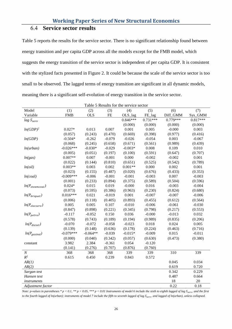
Note: p-values in parentheses * p < 0.1, ** p < 0.05, *** p < 0.01 Instruments of model 6 include the sixth to eighth lagged of lag 𝑆𝑠𝑒𝑟𝑣 , and the first

to the fourth lagged of ln(urban); instruments of model 7 include the fifth to seventh lagged of lag 𝑆𝑠𝑒𝑟𝑣 , and lagged of ln(urban), unless collapsed.


27

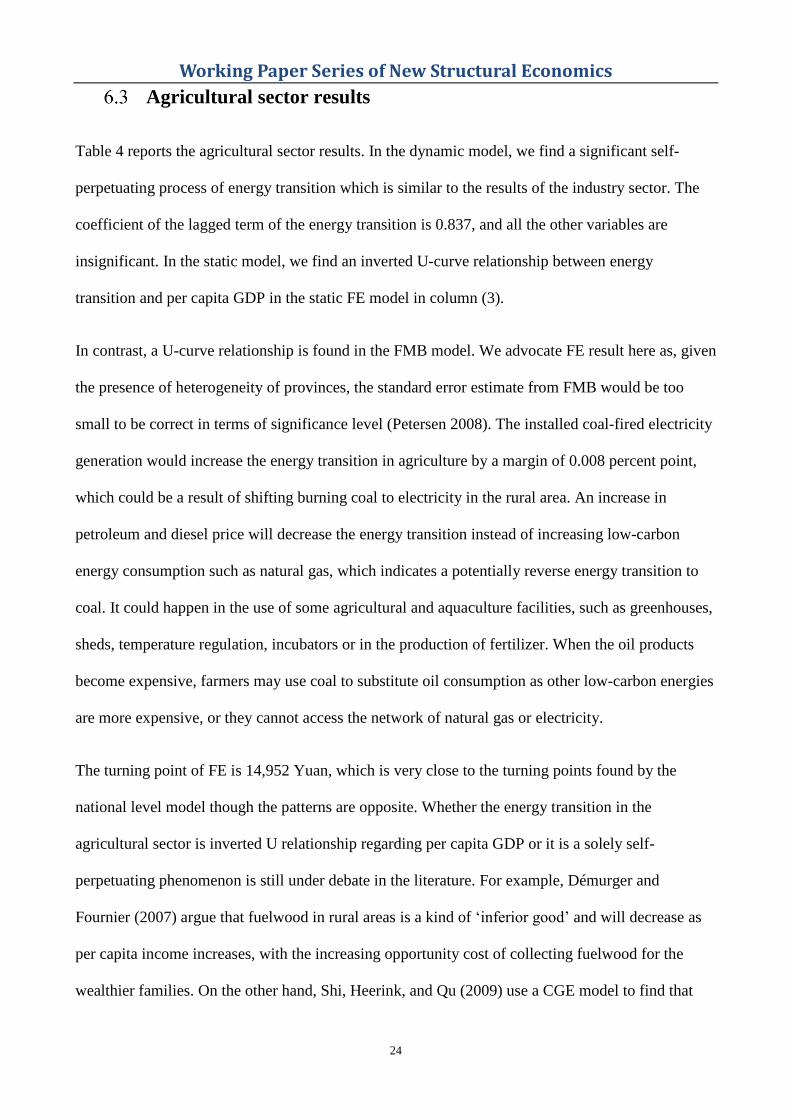
Residential sector results

Results for the residential sector are reported in Table 6. The system GMM model suggests an

inverted U-curve relationship between energy transition and per capita GDP, as the quadratic terms

of per capita GDP are negative (-0.010) and the linear terms are positive (0.221). It indicates that

the low-carbon energy proposition would increase as per capita GDP increases but would

eventually decrease in the long-run as economic growth increases. It is pessimistic, but consistent

with the stylised facts we have found in Figure 2. The turning point is 39,558.94 Yuan suggested by

the system GMM model.

The difference GMM model suggests that oil production has a -0.0219 percent point effect on

energy transition in the long run. It is a sort of natural resource endowment lock-in indicating more

oil endowments would decrease energy transition level in the long run. The FE result shows such

oil endowments effect would be -0.023 percent point in the static model, which is not far different

from the different GMM model.

On the price effect, the system GMM model suggests that diesel oil price has -0.108 percent point

effect on energy transition in the long run. On the other hand, the FE model suggests that the

marginal effect of petroleum price on energy transition is -0.023 percent point. These findings hint

that an increase in such oil product prices seems not decreasing diesel or petroleum consumption in

residential sectors. It could be explained by the correlation between the improvement of living

standards and an increasingly fueled vehicles adoption. The increase in fuel prices is a consequence

of an increase in fueled vehicles consumption rather than a cause of energy transition. It is

consistent with what has been observed in other developing countries such as Botswana (Hiemstra-

van der Horst and Hovorka 2008). Such evidence shows most households prioritize high-carbon

energy consumption rather than shifting to low-carbon fuel use. It could be the underlying reason

9 As we have explained in equation (2), the long-run effect can be computed by the coefficients of control variables divided by the

adjustment factor.


28

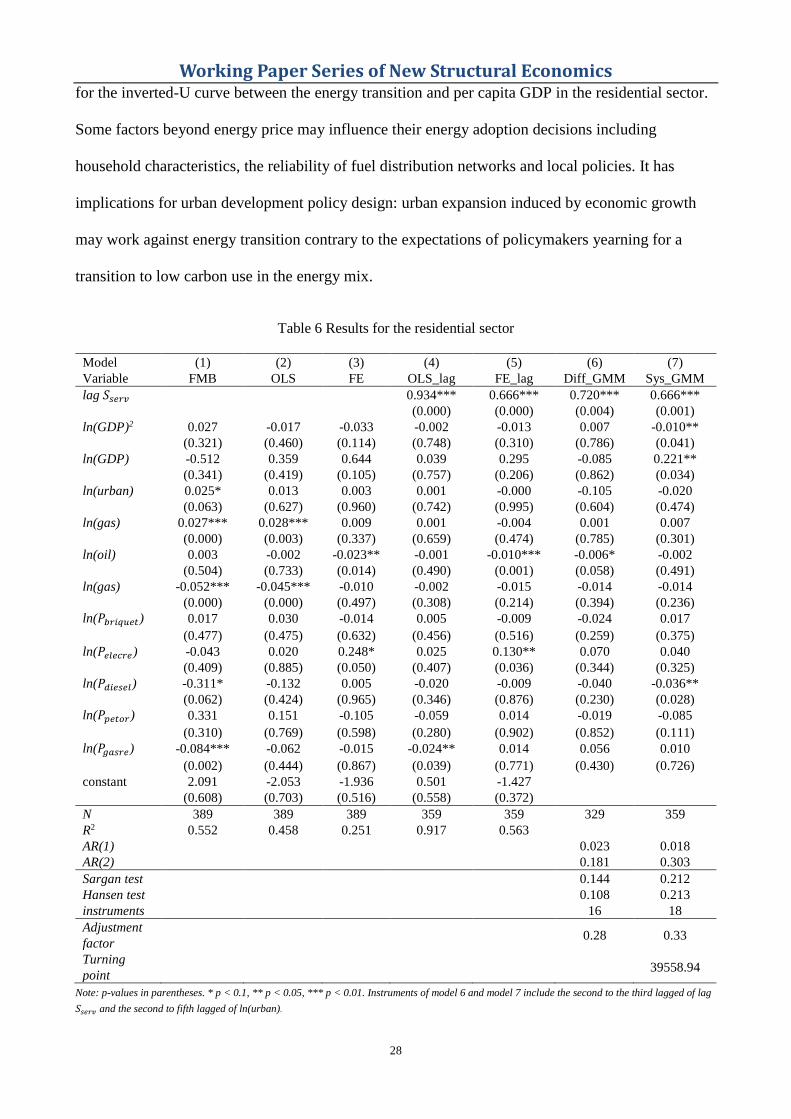
for the inverted-U curve between the energy transition and per capita GDP in the residential sector.

Some factors beyond energy price may influence their energy adoption decisions including

household characteristics, the reliability of fuel distribution networks and local policies. It has

implications for urban development policy design: urban expansion induced by economic growth

may work against energy transition contrary to the expectations of policymakers yearning for a

transition to low carbon use in the energy mix.

Table 6 Results for the residential sector

Model (1) (2) (3) (4) (5) (6) (7)


lag 𝑆𝑠𝑒𝑟𝑣 0.934*** 0.666*** 0.720*** 0.666***

(0.000) (0.000) (0.004) (0.001)

ln(GDP)2 0.027 -0.017 -0.033 -0.002 -0.013 0.007 -0.010**

(0.321) (0.460) (0.114) (0.748) (0.310) (0.786) (0.041)

ln(GDP) -0.512 0.359 0.644 0.039 0.295 -0.085 0.221**

(0.341) (0.419) (0.105) (0.757) (0.206) (0.862) (0.034)

ln(urban) 0.025* 0.013 0.003 0.001 -0.000 -0.105 -0.020

(0.063) (0.627) (0.960) (0.742) (0.995) (0.604) (0.474)

ln(gas) 0.027*** 0.028*** 0.009 0.001 -0.004 0.001 0.007

(0.000) (0.003) (0.337) (0.659) (0.474) (0.785) (0.301)

ln(oil) 0.003 -0.002 -0.023** -0.001 -0.010*** -0.006* -0.002

(0.504) (0.733) (0.014) (0.490) (0.001) (0.058) (0.491)

ln(gas) -0.052*** -0.045*** -0.010 -0.002 -0.015 -0.014 -0.014

(0.000) (0.000) (0.497) (0.308) (0.214) (0.394) (0.236)

ln(𝑃𝑏𝑟𝑖𝑞𝑢𝑒𝑡) 0.017 0.030 -0.014 0.005 -0.009 -0.024 0.017

(0.477) (0.475) (0.632) (0.456) (0.516) (0.259) (0.375)

ln(𝑃𝑒𝑙𝑒𝑐𝑟𝑒) -0.043 0.020 0.248* 0.025 0.130** 0.070 0.040

(0.409) (0.885) (0.050) (0.407) (0.036) (0.344) (0.325)

ln(𝑃𝑑𝑖𝑒𝑠𝑒𝑙) -0.311* -0.132 0.005 -0.020 -0.009 -0.040 -0.036**

(0.062) (0.424) (0.965) (0.346) (0.876) (0.230) (0.028)

ln(𝑃𝑝𝑒𝑡𝑜𝑟) 0.331 0.151 -0.105 -0.059 0.014 -0.019 -0.085

(0.310) (0.769) (0.598) (0.280) (0.902) (0.852) (0.111)

ln(𝑃𝑔𝑎𝑠𝑟𝑒) -0.084*** -0.062 -0.015 -0.024** 0.014 0.056 0.010

(0.002) (0.444) (0.867) (0.039) (0.771) (0.430) (0.726)

constant 2.091 -2.053 -1.936 0.501 -1.427

(0.608) (0.703) (0.516) (0.558) (0.372)

N 389 389 389 359 359 329 359

R2 0.552 0.458 0.251 0.917 0.563

AR(1) 0.023 0.018

AR(2) 0.181 0.303



instruments 16 18

Adjustment

factor

0.28 0.33

Turning

point

39558.94

Note: p-values in parentheses. * p < 0.1, ** p < 0.05, *** p < 0.01. Instruments of model 6 and model 7 include the second to the third lagged of lag

𝑆𝑠𝑒𝑟𝑣 and the second to fifth lagged of ln(urban).

29

7 Policy implication and conclusion

This study investigates the relationship between low-carbon energy transition and economic

growth in China. We use the share of low-carbon energy consumption to measure the degree

of energy transition and per capita GDP is an indicator of economic development. The static

and dynamic panel data models are based on 30 provinces for the period 2000 to 2012 across

four sectors – industry, agriculture, service and residential. We control some factors by the

suggestions of three energy transition hypotheses - the energy ladder, the environmental

Kuznets curve, and carbon lock-in.

At the national level, we find a U-curve relationship between energy transition and economic

development, with the turning point at around 15,350 Yuan at 2010 constant price. It is

consistent with Tahvonen and Salo’s (2001) theoretical model and without losing the

generality of the Environmental Kuznets Curve theory. According to the China National

Bureau of Statistics, all 30 provinces have crossed the turning point so far; thus, generally,

China’s energy mix would continuously decarbonize with further increase of GDP per capita.

It would shed a positive light on China’s future energy transition to low-carbon development.

On the other hand, the patterns at the sectoral level are diverse. We find an inverted U-curve

between energy transition and economic development in the residential sector, with the

turning point appearing around 39,558 Yuan at 2010 constant price. We account this for

increasing use of fuelled vehicles. In the industry sector and service sector, energy transitions

perform a significant autocorrelation of itself. That is, the degree of energy transition largely

depends on the conditions of the energy consumption mix in the previous years. However, the

pattern of the agricultural sector is ambiguous. The static model suggests an inverted U curve

while the dynamic model suggests an autocorrelation process of energy transition. This

30

finding should alert policymakers for the need for more deliberate transition planning and

policy design for households’ level; in particular, electric cars and natural gas-fuelled

vehicles should be encouraged. It also calls for more researches on the agricultural energy

transition.

We find that price effect is significantly effective for promoting energy transition, both

nationally and at sectoral levels. It suggests that the energy market liberalization would be

important for promoting energy transition. After 2005, the price effects became more

significant after 2005. 1% increase in steam coal price will result in 0.093 percent point

increase in energy transition; 1% increase in residential electricity price will increase energy

transition by 0.102 percent point; 1% increase in diesel price will increase low-carbon

proportion by 0.079 percent point, ceteris paribus.

We can also observe a significant natural resource endowment effect. Suggested by the

national level system GMM model, in the long-run, a 1% increase in the natural gas

production will increase low-carbon energy transition by 0.022 percent point in the long run;

a 1% increase in petroleum price will promote energy transition by 0.188 percent point,

ceteris paribus. On the contrary, a long-run effect of 1% increase in industrial electricity

price or industry natural gas price will significantly decrease energy transition by 0.119 and

0.111 percent point, respectively. Suggested by the industry sector FE and difference GMM

models, the natural gas endowment would increase energy transition by 0.010 percent point

and the coal endowment would decrease energy transition by 0.012 percent point at the

margin.

We find that the energy transition could be hindered by too much coal-fired electricity

generation at the national level and the coefficient of 0.016 percent point. Hence, the

31

industrial policy such as reduction coal-fired generation and stimulating renewable electricity

would remove such kind of lock-in effect.

Overall, this paper reveals that the pattern of China’s energy transition varies according to

different levels, different sectors and different stages of economic growth. The marginal

effects of control variables and their driving forces are varying due to natural conditions,

technology progress or institutional reform. The energy transition policy and other relating

industrial policy decision-making should deliberately examine the conditions on a case-by-

case basis.

Acknowledgements

This research is funded by the University of Western Australia UWA - China Scholarship

(No.201308190001), University of Western Australia Top-up scholarship and Postgraduate

Research Grant (PG10100059). It is also partially supported by New Structural Economics

Ph.D. Research Grant from the Institute of New Structural Economics at Peking University,

China. The previous version was presented in the 2nd New Structural Economics Summer

School, 4th International Association for Energy Economics (IAEE) Asian Conference and

30th Chinese Economics Society Australia (CESA) annual conference. It won the runner-up

best student paper award for the IAEE and CESA conferences. Dong Wang expresses

gratitude to the IAEE, the CESA, the College of Public Administration at Huazhong

Agricultural University and the Institute of New Structural Economics at Peking University

for their invitations and travel grants to present this research. We thank Zhiyun Li, Yixiao

Zhou, Ligang Song, Xunpeng Shi, Chunhua Wang for their valuable comments. We are

extremely grateful to the referees. All errors are ours.

References

Anderson, T. W., and Cheng Hsiao. 1981. "Estimation of Dynamic Models with Error Components."

Journal of the American Statistical Association 76 (375):598-606. doi: 10.2307/2287517.

Andreoni, James, and Arik Levinson. 2001. "The simple analytics of the environmental Kuznets

curve." Journal of public economics 80 (2):269-286.

Arellano, Manuel, and Stephen Bond. 1991. "Some Tests of Specification for Panel Data: Monte

Carlo Evidence and an Application to Employment Equations." The Review of Economic

Studies 58 (2):277-297. doi: 10.2307/2297968.

Arthur, W Brian. 1989. "Competing technologies, increasing returns, and lock-in by historical

events." The economic journal:116-131.

Baltagi, Badi H, and James M Griffin. 1984. "Short and long run effects in pooled models."

International Economic Review:631-645.

32

Barnes, Douglas, and Willem Floor. 1996. "Rural energy in developing countries: a challenge for

economic development." Annual Review of Energy and the Environment 21 (1):497-530. doi:

10.1146/annurev.energy.21.1.497.

Barnes, Douglas, and Willem Floor. 1999. "Biomass Energy and the Poor in the Developing World."

Journal of International Affairs 53 (1):237-259.

Barnes, Douglas, and Liu Qian. 1992. Urban interfuel substitution, energy use, and equity in

developing countries: some preliminary results: The World Bank.

Bithas, K., and P. Kalimeris. 2013. "Re-estimating the decoupling effect: Is there an actual transition

towards a less energy-intensive economy?" Energy 51 (0):78-84. doi:

http://dx.doi.org/10.1016/j.energy.2012.11.033.

Blundell, Richard, and Stephen Bond. 1998. "Initial conditions and moment restrictions in dynamic

panel data models." Journal of Econometrics 87 (1):115-143. doi: 10.1016/S0304-

4076(98)00009-8.

Brown, Harrison. 1954. "The challenge of man's future." Engineering and Science 17 (5):16-36.

Brown, Harrison. 1956. "Technological denudation." Man’s Role in Changing the Face of the Earth.

Chicago: University of Chicago:1023-1032.

Brunnschweiler, C. N. 2008. "Cursing the Blessings? Natural Resource Abundance, Institutions, and

Economic Growth." World Development 36 (3):399-419. doi:

10.1016/j.worlddev.2007.03.004.

Burke, Paul J. 2011. "The national–level energy ladder and its carbon implications." Environment

and Development Economics:1-20.

Burke, Paul J. 2012. "Climbing the electricity ladder generates carbon Kuznets curve downturns*."

Australian Journal of Agricultural and Resource Economics 56 (2):260-279. doi:

10.1111/j.1467-8489.2011.00572.x.

Burke, Paul J. 2013. "The National–Level Energy Ladder and its Carbon Implications." Environment

and Development Economics 18 (4):1-20.

Burke, Paul J. 2010. "Income, resources, and electricity mix." Energy Economics 32 (3):616-626.

doi: http://dx.doi.org/10.1016/j.eneco.2010.01.012.

Cameron, A Colin, and Douglas L Miller. 2015. "A practitioner’s guide to cluster-robust inference."

Journal of Human Resources 50 (2):317-372.

Cochrane, John H. 2001. "Fama-MacBeth Procedure." In Asset Pricing, 231. Princeton University

Press.

Crompton, Paul, and Yanrui Wu. 2005. "Energy consumption in China: past trends and future

directions." Energy Economics 27 (1):195-208.

Dasgupta, Susmita, Benoit Laplante, Hua Wang, and David Wheeler. 2002. "Confronting the

environmental Kuznets curve." Journal of economic perspectives:147-168.

Davis, Graham A. 1995. "Learning to love the Dutch disease: Evidence from the mineral economies."

World Development 23 (10):1765-1779. doi: http://dx.doi.org/10.1016/0305-750X(95)00071-

J.

Démurger, Sylvie, and Martin Fournier. 2007. "Rural poverty and fuelwood consumption: Evidence

from Labagoumen Township (China)."

Division, Ministry of Agriculture Science and Technology Education. 2009-2013. China Rural

Energy Statistical Yearbook. Beijing: China Agricultural Publishing House.

Fama, Eugene F., and James D. MacBeth. 1973. "Risk, Return, and Equilibrium: Empirical Tests."

Journal of Political Economy 81 (3):607-636.

Fouquet, Roger. 2010. "The slow search for solutions: Lessons from historical energy transitions by

sector and service." Energy Policy 38 (11):6586-6596. doi:

http://dx.doi.org/10.1016/j.enpol.2010.06.029.

Gales, B., A. Kander, P. Malanima, and M. Rubio. 2007. "North versus South: Energy transition and

energy intensity in Europe over 200 years." European Review of Economic History 11:219-

253. doi: 10.1017/s1361491607001967.

Greene, William H. 2012. Econometric analysis: Pearson Education India.

Grossman, Gene M, and Alan B Krueger. 1991.

Grübler, Arnulf. 2003. Technology and global change: Cambridge University Press.

Grübler, Arnulf. 2004. "Transitions in energy use." Encyclopidia of Energy 6:163-177.

33

Grübler, Arnulf. 2012. "Energy transitions research: insights and cautionary tales." Energy Policy

50:8-16. doi: 10.1016/j.enpol.2012.02.070.

Grübler, Arnulf, Nebojša Nakićenović, and David G Victor. 1999. "Dynamics of energy technologies

and global change." Energy policy 27 (5):247-280.

Guo, Qing King, Chi Keung Marco Lau, Kunwang Li, and Ligang Song. 2015. "National Energy

Market Integration: A study of energy price convergence

in China." In China’s Domestic Transformation in a Global Context, edited by Ross Garnaut Ligang

Song, Fang Cai, Lauren Johnston, 111-135. Canberra, Australia: ANU Press.

Heltberg, Rasmus. 2004. "Fuel switching: evidence from eight developing countries." Energy

Economics 26 (5):869-887.

Herrerias, M., C. Aller, and J. Ordonez. 2017. "Residential energy consumption: A convergence

analysis across Chinese regions." Energy Economics 62:371-381. doi:

10.1016/j.eneco.2016.06.006.

Hiemstra-van der Horst, Greg, and Alice J. Hovorka. 2008. "Reassessing the “energy ladder”:

Household energy use in Maun, Botswana." Energy Policy 36 (9):3333-3344. doi:

https://doi.org/10.1016/j.enpol.2008.05.006.

Hoechle, D. 2007. "Robust standard errors for panel regressions with cross-sectional dependence."

Stata Journal 7 (3):281-312.

Hosier, Richard. 2004. "Energy Ladder in Developing Nations." In Encyclopedia of Energy, 423-435.

Elsevier Science & Technology.

Hosier, Richard, and Jeffrey Dowd. 1987. "Household fuel choice in Zimbabwe: an empirical test of

the energy ladder hypothesis." Resources and Energy 9 (4):347-361.

Hosier, Richard, and W Kipondya. 1993. "Urban household energy use in Tanzania: prices,

substitutes and poverty." Energy Policy 21 (5):454-473.

IPCC. 2018. Spectial Report: Global Warming of 1.5 ºC.

Kander, Astrid, Paolo Malanima, and Paul Warde. 2013. "Power to the People: Energy in Europe over

the Last Five Centuries." Economics Books 1.

Kander, Astrid, Paolo Malanima, and Paul Warde. 2014. Power to the People: Energy in Europe over

the Last Five Centuries: Energy in Europe over the Last Five Centuries. 1 ed: Princeton

University Press.

Kijima, Masaaki, Katsumasa Nishide, and Atsuyuki Ohyama. 2010. "Economic models for the

environmental Kuznets curve: A survey." Journal of Economic Dynamics and Control 34

(7):1187-1201. doi: http://dx.doi.org/10.1016/j.jedc.2010.03.010.

Leach, Gerald. 1988. "Residential Energy in the Third World." Annual Review of Energy 13 (1):47-

65. doi: 10.1146/annurev.eg.13.110188.000403.

Leach, Gerald. 1992. "The energy transition." Energy policy 20 (2):116-123.

Ma, C., and David Stern. 2008. "China's changing energy intensity trend: A decomposition analysis."

Energy Economics 30 (3):1037-1053.

Marcotullio, Peter J, and Niels B Schulz. 2007. "Comparison of energy transitions in the United States

and developing and industrializing economies." World Development 35 (10):1650-1683.

Masera, Omar R, Barbara D Saatkamp, and Daniel M Kammen. 2000. "From linear fuel switching to

multiple cooking strategies: a critique and alternative to the energy ladder model." World

development 28 (12):2083-2103.

NBS. China Price Statistical Yearbook. Beijing: China Statistics Press.

Newey, Whitney K., and Kenneth D. West. 1987. "A Simple, Positive Semi-Definite,

Heteroskedasticity and Autocorrelation Consistent Covariance Matrix." Econometrica 55

(3):703. doi: 10.2307/1913610.

Nickell, Stephen. 1981. "Biases in Dynamic Models with Fixed Effects." Econometrica 49 (6):1417-

1426. doi: 10.2307/1911408.

Palazuelos, E., and C. Garcia. 2008. "China's energy transition: features and drivers." Post-

Communist Economies 20 (4):461-481. doi: 10.1080/14631370802444716.

Petersen, Mitchell A. 2008. "Estimating Standard Errors in Finance Panel Data Sets: Comparing

Approaches." The Review of Financial Studies 22 (1):435-480. doi: 10.1093/rfs/hhn053.

34

Rio, del Pablo, and Gregory Unruh. 2007. "Overcoming the lock-out of renewable energy

technologies in Spain: the cases of wind and solar electricity." Renewable and Sustainable

Energy Reviews 11 (7):1498-1513.

Sachs, Jeffrey, and Andrew Warner. 1995. NBER Working Paper.

Schmalensee, Richard, Thomas M Stoker, and Ruth A Judson. 1998. "World carbon dioxide

emissions: 1950–2050." Review of Economics and Statistics 80 (1):15-27.

Sheehan, Peter, Enjiang Cheng, Alex English, and Fanghong Sun. 2014. "China's response to the air

pollution shock." Nature Climate Change 4:306. doi: 10.1038/nclimate2197.

Shi, X. P., N. Heerink, and F. T. Qu. 2009. "The role of off-farm employment in the rural energy

consumption transition - A village-level analysis in Jiangxi Province, China." China

Economic Review 20 (2):350-359. doi: 10.1016/j.chieco.2008.10.001.

Smil, Vaclav. 2010. Energy transitions: history, requirements, prospects: ABC-CLIO.

Solomon, Barry D., and Karthik Krishna. 2011. "The coming sustainable energy transition: History,

strategies, and outlook." Energy Policy 39 (11):7422-7431. doi:

http://dx.doi.org/10.1016/j.enpol.2011.09.009.

Stern, David. 2004. "Aggregation of energy." In Encyclopedia of energy, edited by Cutler J Cleveland

and Robert K Kaufmann, 17-28. San Diego, CA: Academic Press.

Stern, David, Michael S Common, and Edward B Barbier. 1996. "Economic growth and

environmental degradation: the environmental Kuznets curve and sustainable development."

World development 24 (7):1151-1160.

Stijns, J. P. 2006. "Natural resource abundance and human capital accumulation." World

Development 34 (6):1060-1083. doi: 10.1016/j.worlddev.2005.11.005.

Tahvonen, O., and S. Salo. 2001. "Economic growth and transitions between renewable and

nonrenewable energy resources." European Economic Review 45 (8):1379-1398. doi:

10.1016/s0014-2921(00)00062-3.

Unruh, Gregory. 2000. "Understanding carbon lock-in." Energy policy 28 (12):817-830. doi:

10.1016/S0301-4215(00)00070-7.

Van der Kroon, Bianca, Roy Brouwer, and Pieter J. H. van Beukering. 2013. "The energy ladder:

Theoretical myth or empirical truth? Results from a meta-analysis." Renewable and

Sustainable Energy Reviews 20 (Supplement C):504-513. doi: 10.1016/j.rser.2012.11.045.

Verbeek, Marno. 2012. A Guide to Modern Econometrics. 4 ed: A John Wiley & Sons, Ltd.,.

Wang, Chunhua. 2011. "Sources of energy productivity growth and its distribution dynamics in

China." Resource and Energy Economics 33 (1):279-292.

Wang, Hua, and David Wheeler. 2003. "Equilibrium pollution and economic development in China."

Environment and Development Economics 8 (03):451-466.

Wu, Yanrui. 2003. "Deregulation and growth in China's energy sector: a review of recent

development." Energy Policy 31 (13):1417-1425. doi: http://dx.doi.org/10.1016/S0301-

4215(02)00202-1.

Wu, Yanrui. 2012. "Energy intensity and its determinants in China's regional economies." Energy

Policy 41:703-711.

Zhang, Zhongxiang. 2000. "Decoupling China’s carbon emissions increase from economic growth:

An economic analysis and policy implications." World Development 28 (4):739-752.

35

Appendix

Appendix: Data Supplementary

China’s energy transition between low-carbon energy and high-carbon energy is measured by

the share of low-carbon energy in total energy consumption:

𝑆 =∑ 𝜃𝐿𝐸𝐿𝐿

∑ (𝜃𝐿𝐸𝐿 + 𝜃𝐻𝐸𝐻)𝐿,𝐻 (4)

where S is the share of low-carbon energy; E is the quantity of energy consumption, L

indicates a source of low-carbon energy, and H is a source of high-carbon energy. The term θ

represents a conversion factor used to convert all energy types to the coal equivalent.10 We

use the conversion factor sources from the China National Bureau of Statistics.

We consider ten types of energy: coal, diesel oil, gasoline, kerosene, fuel oil, raw oil,

liquefied petroleum gas (LPG), natural gas, methane, and non-fossil primary electricity which

includes nuclear, hydro, solar and wind as a single unit. Coal and oil products are classified

as high-carbon energy and other types as low-carbon energy. All energy quantities are the

final consumption by end-users, measured in a heat equivalent unit, tonnes of coal equivalent

(TCE). We split energy consumption into four sectors for sectoral level analysis within a

province: industry, agriculture, residential and service.

This study is based on a longitudinal dataset of 30 provinces in China from 2000 to 2012 for

ten types of energy: coal, diesel oil, gasoline, kerosene, fuel oil, raw oil, liquefied petroleum

gas (LPG), natural gas, methane, and non-fossil primary electricity (i.e. nuclear, hydro, solar

and wind). All energy quantities are of the final consumption by end-users, measured in heat

equivalent units. We split provincial total energy consumption into sectoral levels within each

province -the industrial, agricultural, residential (urban) and service sectors. The data are

collected from the yearly provincial energy balance sheets from various editions of the China

Energy Statistical Yearbook and China Rural Energy Statistical Yearbook.

10 The conversion factor can be found in various versions of China Energy Statistical Yearbook.

36

Per capita GDP are from the National Bureau of Statistics and are calculated at constant

prices (base year 2010). We adopt the China GDP deflator published by the World Bank. Per

capita production data of coal, oil and natural gas are collecting from various editions of the

China Energy Statistical Yearbook. Per capita coal-fired power generation capacity data are

collected from State Electricity Regulatory Commission. The population and urbanisation

data are collected from the China National Population Census and China Population and

Employment Statistics Yearbook. We collected Sulphur dioxide emission data from various

versions of the China Statistical Yearbook on Environment.

We include prices for each type of energy, as these will influence energy adoption, so energy

price regulation will be a potential policy lock-in factor for energy transition. China’s reform

and economic transition is characterised by marketization and deregulation, which has

transformed from a central planning economy to a market economy; the energy sector is no

exception. Energy prices cannot be used as a market signal unless the industry is deregulated.

China’s energy prices were controlled by the state before the ‘dual-track’ pricing reforms11

introduced in the 1980s; after 1990, price liberalisation was accelerated and deregulation was

introduced in the energy sector (Wu 2003).

We collected energy price data from the National Development and Reform Commission,

which surveys commodity prices in 36 large cities at ten-day intervals. We used the energy

price in the capital city of each province as a proxy for energy prices in each province. The

yearly price data was derived by averaging all observations within one year. Other price data

were collected from the China Price Statistical Yearbooks. All price and per capita GDP data

are deflated by 2010 using the GDP deflator issued by World Bank.12

11 In China, the government followed dual-track pricing, known as ‘shuangguizhi’ in Chinese. State-controlled (planned)

prices, which were lower, accompanied the market prices, which were higher. This was done to ensure stability and gradual

opening of markets (instead of a ‘big bang’ strategy of sudden transformation to capitalism that was followed in Eastern

Europe and Russia). However, to provide incentive to the State-owned Enterprises, government allowed selling of the

products at market prices after the planned targets had been met. Source: https://en.wikipedia.org/wiki/Dual-track_system. 12 Source: http://data.worldbank.org.cn/indicator/NY.GDP.DEFL.ZS, based year is 2010.

https://en.wikipedia.org/wiki/Dual-track_system

http://data.worldbank.org.cn/indicator/NY.GDP.DEFL.ZS

37

Appendix-table 1 Summary of variables

Variable Label Unit Obs Mean Std.Dev. Min Max

Dependent variables

𝑆 Share of low-carbon energy consumption at national level % 390 0.106 0.110 9.00e-05 0.565

𝑆𝑖𝑛𝑑 Share of low-carbon energy consumption in industrial sector % 390 0.101 0.125 0.000168 0.718

𝑆𝑎𝑔 Share of low-carbon energy consumption in agricultural sector % 390 0.126 0.147 4.17e-05 0.790

𝑆𝑠𝑒𝑟𝑣 Share of low-carbon energy consumption in service sector % 368 0.0543 0.0680 5.84e-05 0.494

𝑆𝑟𝑒 Share of low-carbon energy consumption in residential sector % 389 0.241 0.147 0.0150 0.664

Independent variables

GDP GDP per capita Yuan 390 16291 11200 2662 57132

coalgen Coal generation capacity per capita W 390 423.7 370.8 58.17 2567

urban Urban population 104 390 1912 1259 181 7141

gas Natural gas production per capita 104tce 390 94.24 215.9 0 1145

oil Oil production per capita 104tce 390 0.212 0.420 0 2.566

coal Coal production per capita 104tce 390 2.466 4.986 0 41.84

𝑃𝑏𝑟𝑖𝑞𝑢𝑒𝑡 Briquet price Yuan/100kg 390 35.90 17.52 8.500 99

𝑃𝑠𝑡𝑒𝑎𝑚𝑐𝑜𝑎𝑙 Steam coal price Yuan/ton 390 366.5 181.3 74.10 879.9

𝑃𝑒𝑙𝑒𝑐𝑖𝑛𝑑 Industry electricity price Yuan/kWh 390 0.622 0.147 0.160 0.930

𝑃𝑒𝑙𝑒𝑐𝑟𝑒 Residential electricity price Yuan/kWh 390 0.500 0.0704 0.319 0.879

𝑃𝑒𝑙𝑒𝑐𝑎𝑔 Agricultural electricity price Yuan/kWh 390 0.418 0.108 0.145 0.748

𝑃𝑒𝑙𝑒𝑐𝑠𝑒𝑟𝑣 Service electricity price Yuan/kWh 390 0.790 0.110 0.502 1.043

𝑃𝑝𝑒𝑡𝑟𝑜 93# petroleum price Yuan/ton 390 6190 2273 2898 11247

𝑃𝑑𝑖𝑒𝑠𝑒𝑙 0# diesel price Yuan/ton 390 5306 1914 2548 9052

𝑃𝑔𝑎𝑠𝑖𝑛𝑑 Industry natural gas price Yuan/ton 390 2.304 0.779 0.730 4.600

𝑃𝑔𝑎𝑠𝑟𝑒 Residential natural gas price Yuan/m3 390 2.041 0.540 0.920 3.740

SO2 SO2 emission 104ton 390 73.75 45.11 2 200.3

38

Appendix-table 2 Test for autocorrelation, heteroscedasticity and cross-sectional independence

test National

model

Industry

sector model

Agricultural

sector model

Service

sector model

Residential

sector model

Wooldridge test

for

autocorrelation

0.1234 0.0001 0.0000 0.0003 0.0000

Modified Wald

for groupwise

heteroskedasticity

0.0000 0.0000 0.0000 0.0000 0.0000

Pesaran test for

cross sectional

independence

0.4271 0.6539 0.0000 0.2172 0.6898

Standard error White Roger Driscoll-

Kraay Rogers Rogers

p-value

Date post:	06-Aug-2020
Category:	Documents
Upload:	others
View:	1 times
Download:	0 times

China’s Energy Transition and Economic Growth: A …...energy transition and the energy market...

Documents