+ All Categories
Home > Documents > China’s climate mitigation challenges and tools: essays on ...

China’s climate mitigation challenges and tools: essays on ...

Date post: 02-Jan-2022
Category:
Upload: others
View: 4 times
Download: 0 times
Share this document with a friend
120
China’s climate mitigation challenges and tools: essays on rebalancing, coal-use efficiency and emissions trading A thesis submitted for the degree of Doctor of Philosophy of The Australian National University 27 January 2016 Shenghao Feng Crawford School of Public Policy © Copyright by Shenghao Feng 2016 All Rights Reserved i
Transcript

China’s climate mitigation challenges and

tools: essays on rebalancing, coal-use

efficiency and emissions trading

A thesis submitted for the degree of Doctor of Philosophy of

The Australian National University

27 January 2016

Shenghao Feng

Crawford School of Public Policy

© Copyright by Shenghao Feng 2016

All Rights Reserved

i

Declaration

This thesis is my own original work and contains no material that has been submitted for a

degree at the Australian National University or any other university. It contains no copy or

paraphrase of work published by another person, unless explicitly stated.

An earlier version of Chapter 2 was presented by me at London Metropolitan University.

An earlier version of Chapter 4 was presented by me at Tsinghua University.

An earlier version of Chapter 3 was published as a project output authored by Feng

Shenghao and Mai Yinhua “ Increasing China’s coal-fired power generation efficiency –

impact on China’s carbon intensity.” An earlier version of Chapter 4 was published as a

journal article authored by Liu Yu, Feng Shenghao, Cai Songfeng, Zhang Yaxiong, Zhou

Xiang, Chen Yabin and Chen Zhanming “Carbon emissions trading system of China: a

linked market vs. separated markets”, Frontiers of Earth Science, 2013, 7(4): 465-479. Both

Chapters 3 and Chapter 4 contain significant new material and analysis conducted by me.

All errors in this thesis are my own responsibility.

Shenghao Feng

27 January 2016

i

Acknowledgement

I would like to take this opportunity to express my deepest gratitude to those who have

helped me during this journey. This thesis would not have been finished without your

support.

First, I would like to thank Professor Stephen Howes. Stephen took me on board, helped

me find a topic, encouraged me to learn CGE modelling, gave me the opportunity to be a

tutor, tore my drafts apart and helped me put them back together. I thank you for your

guidance, patience, and generousity.

Second, I would like to thank Associate Professor Frank Jotzo. Frank gave me the

opportunity to work with him first as a research assistant, then as a co-author. The things I

learned from him gave me confidence, and helped me to develop my skills and to realize

my passion.

Third, I would like to thank Dr Mai Yinhua and Dr Liu Yu, with whom I developed key parts

of this thesis.

Fourth, I owe special thanks to Professor Philp Adams, Dr Peng Xiujian and all the staff and

students at the Centre of Policy Studies. You taught me everything I could have wished for

about CGE modelling and more. You are a truly warm and generous community.

Last but not least, I thank my wife, my parents and my parents in law. You know all the

difficulties I have had and helped me overcome all of them; you know the progress I have

made and shared every happy moment with me. Your encouragement, patience, sacrifice

and above all love gave me strength.

ii

Abstract

The contribution of this thesis lies in its original application of Computable General

Equilibrium (CGE) modelling to some of the most important climate change mitigation

challenges China faces, and some of the tools it could use to overcome them. The original

findings of the thesis are summarized below. Overall, they underline the need for China to

implement new methods, carefully designed, to reduce emissions.

Chapter 2 focuses on the challenge of China’s economic structure, and the tool of

restructuring. A two-stage estimation process is implemented within CHINAGEM, a

dynamic general equilibrium model of the Chinese economy, to study the potential

contribution of successful economic rebalancing – from investment to consumption, and

from industry to services – to reducing the country’s carbon dioxide emissions. The results

show that economic rebalancing alone may lead to 17 per cent reduction in the emissions

intensity of GDP between 2012 and 2030. This estimate is higher than existing partial

equilibrium estimates in the literature, and points to the importance of economic

rebalancing from an environmental perspective.

Chapter 3 focuses on the challenge of China’s heavy level of coal dependency, and the tool

of improving the efficiency of the use of coal in power generation. The analysis, again

based on CHINAGEM, suggests that this will be a less important contributor to mitigation

in the future than in the past. The pace and importance of improvements in coal-fired

power generation efficiency is projected to halve mainly because, after the progress

already made, China’s current coal-fired power generation efficiency is already close to

the world’s best practice, but also because slower growth in electricity demand reduces

the scope for expanding the generation fleet with new world-class plant. The chapter also

shows that, going forward, switching to renewable energy and structural rebalancing will

be more important for achieving China’s emissions targets than improving coal-fired

iii

power generation efficiency. However, fully achieving China’s 2020 emissions intensity

reduction target will require a combination of all three.

Chapter 4 focuses on the challenge of China’s enormous regional diversity, and the tool of

emissions trading. This chapter uses a multi-provincial static CGE model of the Chinese

economy, SinoTERM-CO2, to simulate the linking of two provinces through a single

emissions trading scheme. The simulations show that the richer regions (typified by

Guangdong) may benefit from linking but the poorer regions (typified by Hubei) may lose.

This is because poorer provinces in China tend to be more emissions intensive and

therefore likely to face a carbon price rise upon linking, the economy-wide costs of which

may be only partially offset by trading, if indeed trading is permitted. The economic logic

behind this is explained by improving on the stylized model suggested by Adams and

Parmenter (2013). China has not yet decided whether provincial caps will be retained

when a national emissions trading scheme is introduced. This analysis suggests that they

should be retained, and made more generous for poorer regions in order to ensure that

linking is both welfare enhancing and politically acceptable.

iv

Table of contents

Chapter 1 Introduction .................................................................................................... 1

1.1 Introduction ...............................................................................................................................1

1.2 Literature review and models ....................................................................................................2

1.3 Guide to the chapters ................................................................................................................4

1.4 Contribution of the thesis ..........................................................................................................5

Chapter 2 Economic rebalancing and carbon dioxide emissions .......................................... 7

2.1 Introduction ...............................................................................................................................8

2.2 Background: imbalances, concerns, causes and remedies ........................................................9

2.3 Modelling the link between rebalancing and emissions: literature survey and approach ..... 23

2.4 Simulation results ................................................................................................................... 29

2.5 Concluding remarks ................................................................................................................ 34

Chapter 3 Efficiency improvements in coal-fired power generation and emissions reduction ..................................................................................................................... 37

3.1 Introduction ............................................................................................................................ 38

3.2 A method to project China’s coal-fired efficiency improvement ........................................... 42

3.3 The CGE model, generic assumptions and the base case scenario ........................................ 45

3.4 Projecting China’s coal-fired efficiency improvement and its importance............................. 48

3.5 Assessing the relative roles of rebalancing, renewable energy and efficiency improvement 51

3.6 Discussion and conclusion ...................................................................................................... 56

Chapter 4 Linking regional carbon markets in China: analyzing efficiency and equity impacts ........................................................................................................................ 61

4.1 Introduction ............................................................................................................................ 62

4.2 Literature review ..................................................................................................................... 63

4.3 Challenges of ETS linking in China ........................................................................................... 65

4.4 Model, provinces and scenarios ............................................................................................. 68

4.5 Simulation results ................................................................................................................... 72

4.6 Discussion ................................................................................................................................ 77

4.7 Conclusion ............................................................................................................................... 90

Chapter 5 Conclusion .................................................................................................... 93

v

List of tables

Table 2.1: China’s current account balance ......................................................................... 10

Table 2.2: Health and education expenditure shares, a worldwide comparison ................ 15

Table 2.3: Public health and education expenditures, a worldwide comparison ............... 15

Table 2.4: Energy intensity and fossil fuel dependency, a worldwide comparison, 2010 ... 22

Table 2.5: Baseline and policy scenario economic structures, 2030 ................................... 26

Table 2.6: Closure for both the baseline and policy scenario .............................................. 27

Table 2.7: GDP and factor growth, cumulative percentage deviation by 2030 .................. 29

Table 2.8: Demand side of GDP, cumulative percentage deviation by 2030 ...................... 30

Table 2.9: Sector output, prices and input demand, , cumulative percentage deviation by 2030 ...................................................................................................................................... 31

Table 2.10: Sectoral value-added, carbon dioxide emissions and emissions intensity index, 2030 ...................................................................................................................................... 33

Table 3.1: Composition of China’s coal-fired power generation fleet, 2010 ....................... 43

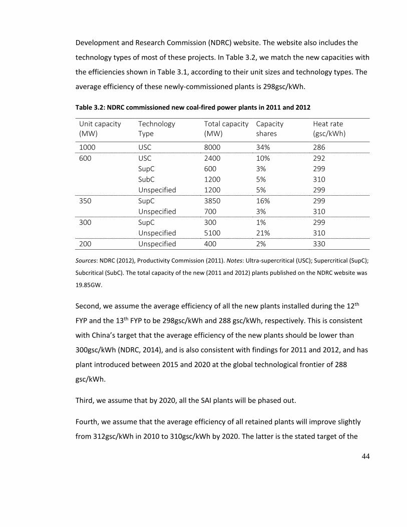
Table 3.2: NDRC commissioned new coal-fired power plants in 2011 and 2012 ................ 44

Table 3.3: Macroeconomic structure and electricity generation by fuel, base case scenario .............................................................................................................................................. 46

Table 3.4: Key simulation results under the base case scenario, cumulative % growth. .... 47

Table 3.5: Coal-fired power generation capacity composition and heat rate, 2010 (actuals) and 2020 (base case). ........................................................................................................... 49

Table 3.6: Actual and projected coal-fired power generation efficiency ............................ 49

Table 3.7: Emissions, real GDP and emissions intensity of GDP, cumulative percentage deviation in 2020 from improvements in coal-fired power efficiency. ............................... 50

Table 3.8: Macroeconomic structure, sectoral composition, and the fuel mix in the electricity generation sector – alternative assumptions for 2020. ...................................... 52

Table 3.9: New planned capacity (GW) and heat rate (gsc/kWh) ....................................... 53

Table 3.10: Emissions, real GDP and emissions intensity of GDP under the different scenarios .............................................................................................................................. 54

vi

Table 3.11: Cumulative % change in emissions intensity 2005-20 ...................................... 54

Table 3.12: Emissions, real GDP and emissions intensity of GDP under the different scenarios: the impact of coal efficiency alone ..................................................................... 55

Table 3.13: Coal-fired power generation efficiency: 2010 and possible 2020 scenarios .... 56

Table 3.14: The contribution of coal-fired power generation efficiency to emissions intensity reduction: 2005-2012 and 2012-2020 .................................................................. 57

Table 4.1: Emissions, GDP, emissions intensity of GDP, regional intensity reduction targets, and average carbon price levels, China’s pilot ETSs ............................................................ 65

Table 4.2: Caps under moderate and ambitious mitigation variants .................................. 70

Table 4.3: Cap assumptions in the four scenarios ............................................................... 72

Table 4.4: Main simulation outputs for the moderate mitigation variant .......................... 76

Table 4.5: Main simulation outputs for the ambitious mitigation variant .......................... 76

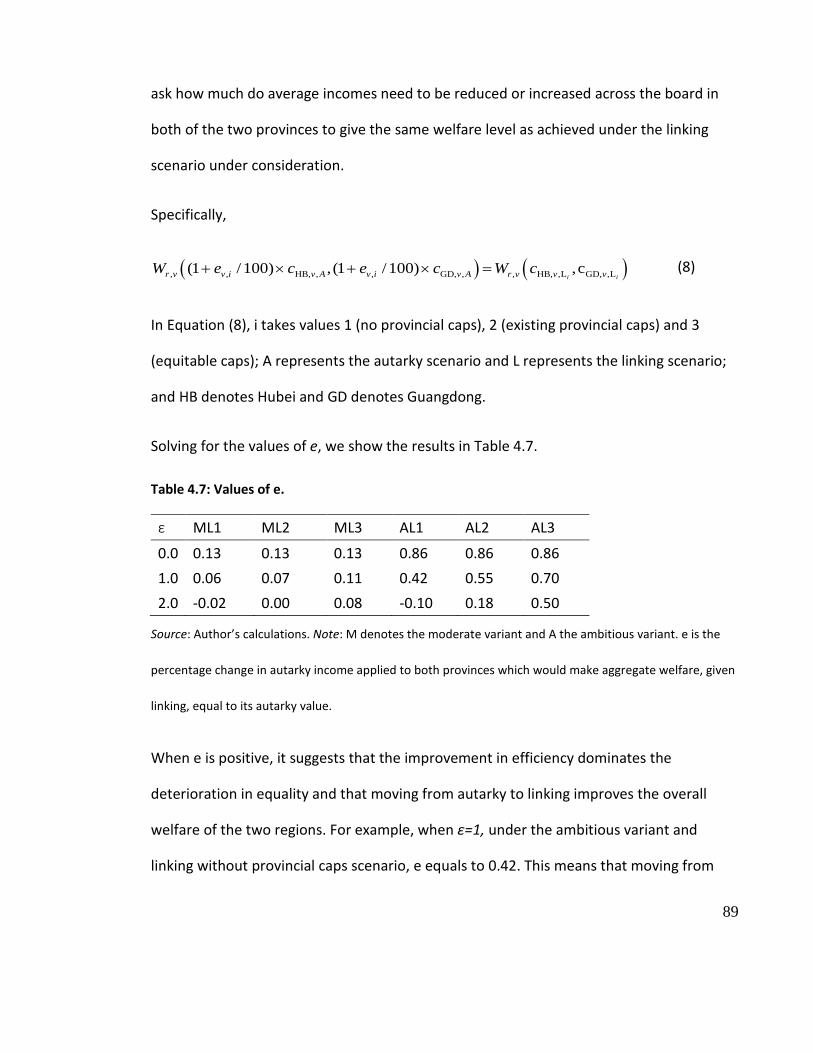
Table 4.6: Elements on the right hand side of Equation (3) ................................................ 80

Table 4.7: Values of e. .......................................................................................................... 89

vii

List of figures

Figure 2.1: consumption/investment (C/I) ratio, China in the world .................................. 10

Figure 2.2: Service/industry sectoral value added ratio, China in the world ...................... 11

Figure 2.3: Relationship between investment and industry share in GDP, for different groups of countries between 1980 and 2010 ...................................................................... 17

Figure 2.4: China’s carbon dioxide emissions in a global context ....................................... 20

Figure 2.5: Carbon emissions intensity of GDP, China in the world .................................... 21

Figure 2.6: Emissions intensity and heavy industry ............................................................. 22

Figure 2.7: China benchmark interest rate between Janurary 2002 and January 2014 ...... 30

Figure 3.1: Coal-fired power plants efficiency: standard coal per kilowatt-hour electricity supply to the grid† ................................................................................................................ 39

Figure 3.2: Carbon intensity, energy intensity and coal-fired power generation efficiency in China ..................................................................................................................................... 40

Figure 3.3: Coal-fired power generation capacity composition, 2010 (actuals) and 2020 (base case). ........................................................................................................................... 48

Figure 4.1: Emissions intensity versus GDP per capita, China’s provinces, 2007. ............... 66

Figure 4.2: Emissions intensity, GDP per capita and abatement targets and of China’s provinces. ............................................................................................................................. 67

Figure 4.3: Absolute emissions reduction targets and GDP per capita, EU-15, 2008-2012 67

Figure 4.4: Guangdong and Hubei autarky (a) emissions abatement and (b) real GDP cost at various permit prices (CNY per ton)................................................................................. 71

Figure 4.5: Percentage reduction in real GDP at factor cost, autarky, modelled versus stylized. ................................................................................................................................ 81

Figure 4.6: Emissions intensity versus capital-labour ratio by sectors. ............................... 82

Figure 4.7: % change in real sectoral output versus sector capital-labour ratio under autarky, moderate mitigation variant .................................................................................. 83

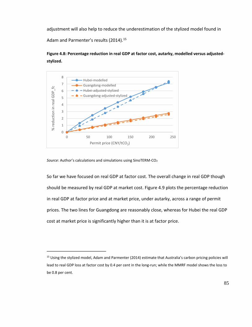
Figure 4.8: Percentage reduction in real GDP at factor cost, autarky, modelled versus adjusted-stylized. ................................................................................................................. 85

viii

Figure 4.9: Percentage reduction in real GDP at factor cost versus at market price, autarky. .............................................................................................................................................. 86

Figure 4.10: Percentage change in real GDP versus pre-existing, sectoral tax shares under Autarky, moderate mitigation variant. ................................................................................ 87

ix

Chapter 1 Introduction

1.1 Introduction

Energy conservation, emissions reduction and environmental conservation – or, what this

thesis refers to as climate change mitigation – are increasingly important priorities for the

Chinese government. China is the largest carbon dioxide (CO2) emitter in the world and

fossil fuel combustion is by far the largest source of carbon dioxide emissions in China.

China needs to control the use of fossil fuels for a number of compelling reasons. First, the

burning of fossil fuels is a main cause of China’s domestic air pollution, a threat to social

stability and sustainable development. Second, a high dependency on fossil fuel imports

threatens energy security. Third, carbon dioxide emissions are responsible for global

climate change, to which China is vulnerable.

The central government has set multiple emissions targets. In 2009, China committed to

reducing emissions intensity of GDP by 40 to 45 per cent between 2005 and 2020. The 12th

Five Year Plan aimed to cut emissions intensity by 17 per cent between 2010 and 2015.

And in 2015, China’s Intended Nationally Determined Contribution (INDC) submitted to

the United Nations Framework Convention on Climate Change includes a target to reduce

emissions intensity of GDP by 60 to 65 per cent by 2030 form the 2005 level. The INDC

also announced China’s intention for CO2 emissions to peak in 2030 or earlier.

The progress since 2005 has been encouraging. Emissions intensity fell by 24 per cent

from 2005 to 2012 –an average 4 per cent reduction per annum. If such trends can be

sustained, by 2020, emissions intensity will be 48 per cent lower than it was in 2005,

exceeding the upper 45 per cent target. However, progress in the past is no guarantee of

future success. It will arguably become more difficult to reduce emissions intensity over

1

time (once the low-hanging fruits have been picked), so there is no guarantee that the

past trends can be maintained.

This thesis uses computable general equilibrium modelling to examine three challenges

that China will face in the coming years in its quest to reduce emissions, and

correspondingly three tools that it can use to address these challenges: first, the challenge

of economic imbalance, and the tool of rebalancing (Chapter 2); second, the challenge of

coal-dependency and the tool of improving coal-use efficiency (Chapter 3); and third the

challenge of regional diversity, and the tool of emissions trading (Chapter 4).

The next section provides a brief literature review (more detailed reviews can be found in

each of the three chapters) and an introduction to the models used by the thesis. Section

3 provides a guide to each of the three chapters. The concluding section of this chapter

discusses the contribution of this thesis. Summaries of the thesis’ results can be found in

the Conclusion (Chapter 5) and in the abstract at the start of the thesis.

1.2 Literature review and models

Due to the large scale of China’s emissions and their fast rate of growth, climate change

mitigation in China has become a topical issue in the literature. The latest International

Energy Agency’s (IEA) flagship report, Energy Technology Perspectives 2015, projects that

under its 6 degree, 4 degree and 2 degree scenarios, China’s CO2 emissions (from fuel

combustion) will peak after 2050, around 2035 (at around 12 billion tons) and around

2020 (at around 10.7 billion tons), respectively. Yuan et al. (2014) and Wu (2014), both

based on stylized analytical frameworks, draw similar conclusions to IEA’s 4 degree and 6

degree scenarios, respectively.

He (2013) was the first study to argue China could peak emissions by 2030. This was an

important study as it might have helped China to determine its INDC commitments. In

wake of the “new normal” of economic growth, many recent studies have formed a new-

2

found optimism that China might achieve peak emissions before 2025 (Energy Research

Institute, 2015, Garnaut, 2014, Green and Stern, 2015).

Many studies have utilized CGE models to investigate various issues in climate change

mitigation in China. Zhang (1996) and Garbaccio et al. (1999) are two of the earliest

studies that used CGE models to simulate the impact of carbon pricing policies in China.

More recently, Li et al. (2014) investigated the impact of carbon pricing under regulated

electricity price regime and with different revenues-recycling mechanisms. Jiang and Lin

(2014) is another important study that modelled the impact of the removal of energy

subsidies in China. Researchers at the Tsinghua University have also produced several

important works on overall emissions projection (Zhang et al., 2014), renewable energy

development (Qi et al., 2014b) and the relationship between economic restructuring and

trade-embodied emissions (Qi et al., 2014a).

While CGE modelling has been deployed in relation to various climate mitigation issues

and topics, there are still key issues where modelling is required. The topics for this thesis

were selected partly because of their emerging importance, and partly because, as shown

in the various chapters’ individual literature reviews, they are ones where there has been

relatively little modelling and analysis.

There are various CGE models that can be and have been used to examine climate change

policies. This thesis uses two well-respected and well-documented CGE models. The first is

a single country, recursive dynamic model, namely CHINAGEM (Mai et al., 2012, Dixon and

Rimmer, 2002). The core theories of the model are based on the MONASH model (Dixon

and Rimmer, 2007). An emission accounting framework and an energy accounting

framework are incorporated into CHINAGEM as is done in the MMRF model (Adams and

Parmenter 2013) A documentation of CHINAGEM can be found in Mai et al. (2010). The

second is a multi-provincial, static model, namely SinoTERM-CO2 (Horridge and Wittwer,

2008, Horridge, 2012), an upgraded version of SinoTERM (Horridge and Wittwer, 2008) – a

3

China version of the generic TERM model (Horridge et al., 2005). More information on the

two models can be found in Chapters 2 and 4 respectively.

1.3 Guide to the chapters

Each of the main chapters deals with a specific combination of challenges and

corresponding policy tools.

Chapter 2 focuses on the challenge of China’s economic structure, and the tool of

rebalancing. China has grown rapidly from a low-income country to an upper-middle

income country. This was largely achieved by a capital- and emissions-intensive growth

model. However such a growth model has also resulted in rapid growth in CO2 emissions.

Many signs are pointing to the fact that the past growth model is unsustainable. While the

need for rebalancing is now widely acknowledged, and indeed efforts to rebalance are

well underway, there has been little analysis, and no general-equilibrium analysis, to

understand the impact of rebalancing on emissions. This chapter fills the gap by analyzing

the causes and consequences of the imbalances, and the reforms required to rebalance

the Chinese economy. It then models the impact on emissions of rebalancing the economy

in line with the well-known World Bank-DRC China 2030 recommendations. It compares

the results to existing projections based on partial equilibrium analysis.

Chapter 3 focuses on the challenge of China’s heavy level of coal dependency, and the tool

of improving the efficiency of the use of coal in power generation. Power generation is the

major use of coal in China, and coal-fired power plants were responsible for half of the

total CO2 emissions in China in 2012. Traditionally, improving the efficiency of these power

plants has been one of the main ways in which China has reduced its emissions intensity.

For example, improving coal-fired efficiency has been responsible for almost one-quarter

of the reduction in China’s emissions intensity between 2005 and 2010. This chapter asks

what the scope is for further improvements in coal-fired efficiency out to 2020, and

4

whether such improvements can play a big a role in the future as they have in the past.

Since, to anticipate the results, the answer is negative, the chapter also builds on the

results of the previous one by comparing the relative importance of improving coal-fired

efficiency with that of structural rebalancing and of diversifying to renewables.

China has not so far made much use at all of pricing instruments in its quest for emissions

reduction. It has relied far more on administrative measures and targets. However, again,

the future is unlikely to be like the past, and China has set up seven Emissions Trading

Scheme (ETS) pilots and is looking to establish a national ETS from 2017.

Chapter 4 focuses on the challenges of China’s enormous regional diversity, and the tool

of emissions trading. Chapter 4 explores this issue by using a single country, multi-regional

CGE model of China to simulate the linking of the carbon markets in a representative

better-off and less emissions-intensive province, Guangdong, and a poorer, more

emissions-intensive, Hubei. (In general, in China, the poorer economies are more

emissions-intensive.) Including only two provinces makes the exercise tractable while still

allowing implications to be drawn for a nationwide ETS. The chapter examines the

implications of linking for the two provinces and for overall welfare, and compares results

when existing provincial targets are abolished, retained, or modified to be made more

progressive. The chapter also tests a “rule of thumb” or stylized model put forward by

Adams and Parmenter (2013) to understand the GDP impact of changing the carbon

prices, and suggests a modification to it based on the results obtained.

1.4 Contribution of the thesis

This thesis make several distinct and original contributions. First, it applies CGE modelling

to three new and important climate change mitigation challenges to come up with new

findings and consequent policy recommendations (as summarized in the concluding

chapter, Chapter 5). Second, in Chapters 2 and 3 it develops and utilizes a new technique

5

for modelling rebalancing and changes in the energy composition. Third, in Chapter 3, the

thesis provides a new projection of potential coal-use power generation efficiency. This

method could also be deployed in other sectors, such as aluminum and steel. Fourth, in

Chapter 4, the thesis proposes a new stylized model, improving on the proposal of Adams

and Parmenter (2013) to better understand the economy-wide impact of carbon pricing.

While there are a number of limitations to the modelling techniques deployed (set out in

each chapter and summarized in Chapter 5), overall the thesis shows the value of

deploying general equilibrium model to understand the economy-wide impact of major

and complex economic reforms. It is hoped that the contributions of this thesis are

beneficial to both academics and policy-makers alike.

6

Chapter 2 Economic rebalancing and carbon

dioxide emissions

Abstract

China needs to rebalance away from investment, exports and industry to consumption

and services. Since the old growth model is energy- and emissions-intensive, shifting to a

new growth model could have profound implications for China’s carbon dioxide emissions.

This paper uses a general equilibrium model to study the potential impact of successful

economic rebalancing in China on the country’s carbon dioxide emissions. The results

show that economic rebalancing alone may, by 2030, lead to a 17 per cent reduction in

the emissions intensity of GDP. Although this result can only be regarded as indicative, it is

higher than existing estimates based on partial equilibrium analysis, and it shows the

importance of economic rebalancing to China’s climate change response.

7

2.1 Introduction

China’s economy has been growing rapidly over the past 30 years. This has transformed

the country. In 1981, 84 per cent of the population lived at below USD1.25 (PPP adjusted)

a day; by 2009 that ratio had fallen to 12 per cent (WDI, 2013). Urbanization rose from

below 20 per cent in late 1970s to more than 50 per cent in early 2010s (ibid). China

became a lower-middle-income country in 1997 and a higher-middle-income country in

2010 (ibid). It is now the second largest economy in the world.

However, China’s fast growth has also led to the accumulation of structural problems. Its

economy is unbalanced. The share of consumption (public plus private, hereafter) in GDP

(50 per cent) is the lowest in the world, and its share of investment (46 per cent) the

highest. Both the service sector and the industry sector make up 45 per cent of total

value-added, making the former unusually low and the latter unusually high. Not only is

China’s growth unbalanced, it is also dirty. China consumes the largest amount of energy

in the world – 20 per cent of the global total. China is also the world’s largest carbon

dioxide emitter. In 2009 it contributed a quarter of the world’s total carbon dioxide

emissions.

There is a consensus in China that fundamental change is required to address these

structural problems. The official economic policy position is one of rebalancing. The aim is

to increase the share of consumption to GDP, and of the service sector. The official

environmental policy position is one of reducing both local pollution and carbon dioxide

emissions, at least relative to GDP growth.

To date, the link between these two goals has not received much attention. Yet prima

facie one would expect one goal to affect the other, in particular because the industrial

sector is more carbon-intensive than the service sector.

8

This paper uses a quantitative approach to investigate the potential contribution of

economy-wide rebalancing policies to China’s climate change mitigation. Section two

reviews the imbalances and their causes, remedies and links with carbon emissions.

Section three develops two growth scenarios and a 2-stage simulation used to model

these two scenarios. Section four interprets the simulation results. Section five makes

some concluding remarks.

2.2 Background: imbalances, concerns, causes and remedies

This section examines, in successive sub-sections, China’s main economic imbalances,

their causes, the concerns they have given rise to, their future trajectory and reforms to

reduce them, and, finally, the link between economic rebalancing and the country’s

carbon dioxide emissions.

China’s economic imbalances

There are three major imbalances in China’s economic structure. First, China has a high

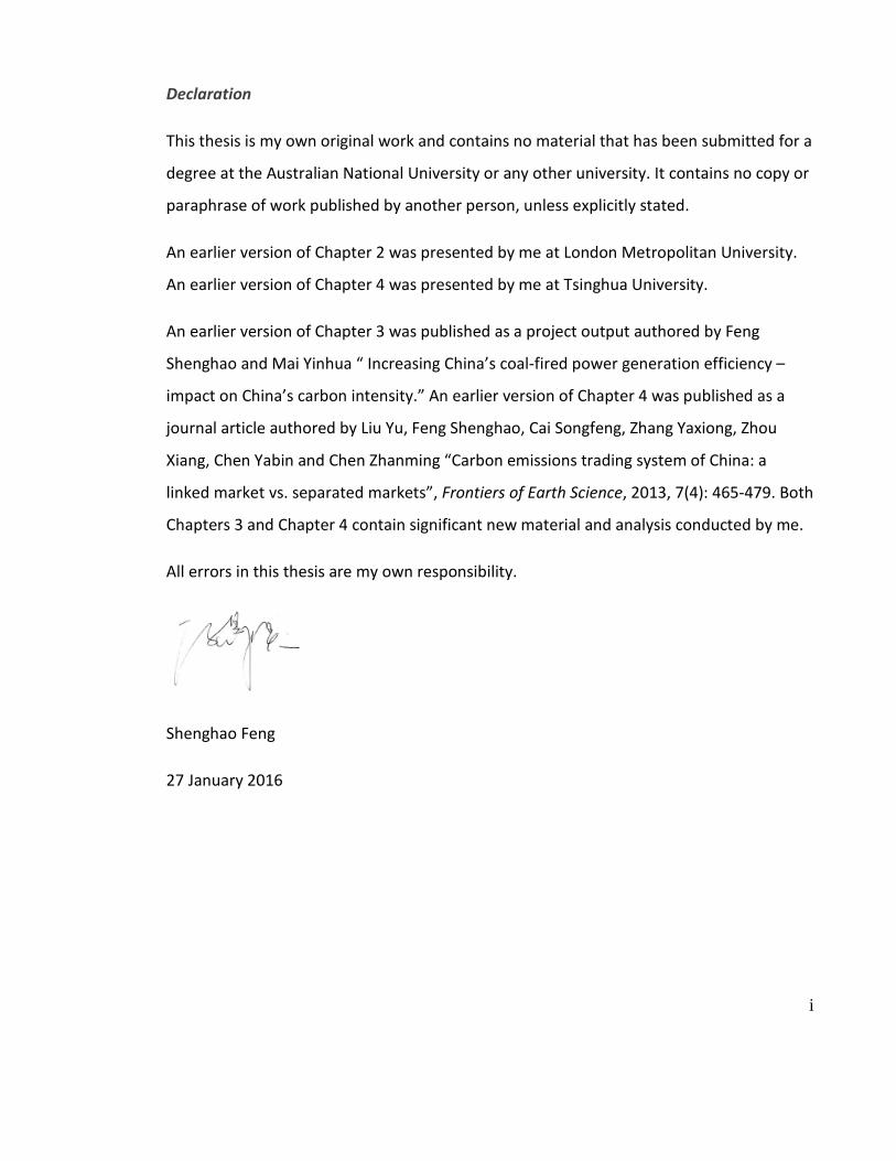
share of investment and a low share of consumption. As Figure 2.1 shows, not only is

China’s consumption/investment (C/I) ratio consistently lower than the world average, but

the difference is increasing. At the beginning of the 1980s, China’s C/I ratio was 1.85 and

the world average was 2.85. By 2011, China’s C/I ratio has fallen to 0.98 whereas the

world average has increased to 3.02.

9

Figure 2.1: consumption/investment (C/I) ratio, China in the world

Source: (WDI, 2013). Note: CHN, HIC, MIC and WLD denote China, high-income-country, middle-income-

country and world, respectively.

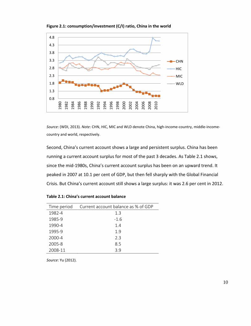
Second, China’s current account shows a large and persistent surplus. China has been

running a current account surplus for most of the past 3 decades. As Table 2.1 shows,

since the mid-1980s, China’s current account surplus has been on an upward trend. It

peaked in 2007 at 10.1 per cent of GDP, but then fell sharply with the Global Financial

Crisis. But China’s current account still shows a large surplus: it was 2.6 per cent in 2012.

Table 2.1: China’s current account balance

Time period Current account balance as % of GDP 1982-4 1.3 1985-9 -1.6 1990-4 1.4 1995-9 1.9 2000-4 2.3 2005-8 8.5 2008-11 3.9

Source: Yu (2012).

0.8

1.3

1.8

2.3

2.8

3.3

3.8

4.3

4.8

1980

1982

1984

1986

1988

1990

1992

1994

1996

1998

2000

2002

2004

2006

2008

2010

CHN

HIC

MIC

WLD

10

Third, China has a large industry sector and a small service sector by world standards.

Figure 2.2 compares China’s service/industry (S/I) ratio with the world average. Again, not

only does China have a consistently lower S/I ratio than the world average, but the gap is

growing. In 1980 China’s S/I ratio was 0.45 and the world average was 1.54. By 2010,

China’s S/I ratio moved up to 0.92. However the world average increased to 2.70.

Figure 2.2: Service/industry sectoral value added ratio, China in the world

Source: WDI (2013). Note: CHN, HIC, MIC and WLD denote China, high-income-country, middle-income-

country and world, respectively.

China’s economic imbalances as causes for concern

Concerns around China’s economic imbalances revolve around eight points. The first is

simply that they are highly unusual by world standards. This does not in itself demonstrate

that they are sub-optimal. However, international comparisons are instructive. Huang and

Wang (2010b) estimated that China’s investment share of GDP could be 20 per cent

higher than the ‘international optimal level’1 and its consumption share 20 per cent lower

(p.295).

1 This is the optimal level estimated by Chenery and Syrquin (1975) from a 101-country database.

0.4

0.9

1.4

1.9

2.4

2.9

3.4

1980

1982

1984

1986

1988

1990

1992

1994

1996

1998

2000

2002

2004

2006

2008

2010

CHN

HIC

MIC

WLD

11

The second is that the imbalances may increase China’s risks. Historical experience

suggests that fast-growing countries powered by high investment levels are prone to

shocks (Pettis and Lardy, 2012). The Asian Financial Crisis is one such episode. On the one

hand China’s economy may be subject to less external shock than its East Asian neighbors

as it does not have an open capital account. But on the other hand, China’s over-

investment is even larger than the estimated over-investment in the other Asian

economies leading up to the Asian crisis (Lee et al., 2012, p.16).

Third, and more fundamentally, high investment coupled with low returns makes growth

unsustainable. China’s rising capital-output ratio indicates falling capital productivity (Qin

et al., 2006). China recorded an improvement in investment efficiency in the first two

decades of reform (Zhang, 2003, p.731),2 but the trend was reversed sometime in the

1990s (Barnett and Brooks, 2010). Although China’s return on capital has been found to

be comparatively healthy by world standards (Bai et al., 2006), it may be on a dynamically

inefficient path (Rawski, 2002). If China’s growth relies increasingly on investment but

investment becomes decreasingly efficient, it is building up trouble (Prasad, 2007, p.1).

Fourth, investment is misallocated at the micro level. Large excess capacities have built up

in heavy-industry sectors such as high-end property, steel, cement, coke and aluminum

(Lardy, 2007, p.7). Even if there is no clear-cut answer as to whether China is over-

investing at the macro-level (Ding et al., 2010, p.6), sectoral misallocations may have been

the main reason for the declining productivity growth for the overall economy (Blanchard

and Giavazzi, 2006, p.7).

Fifth, the low and declining share of consumption is a concern in itself. Fukumoto and

Muto (2012, p.66) argue that giving households a better return from growth is the

foremost rationale for rebalancing China’s economy. Even if China could be excused for

not paying enough dividends (in terms of consumption) to its households (the ultimate

2 Zhang used data between 1980 and 2000.

12

shareholders) when investment opportunities were more profitable in the earlier years of

the reform, it should certainly be paying more dividends now that investment returns

have fallen.

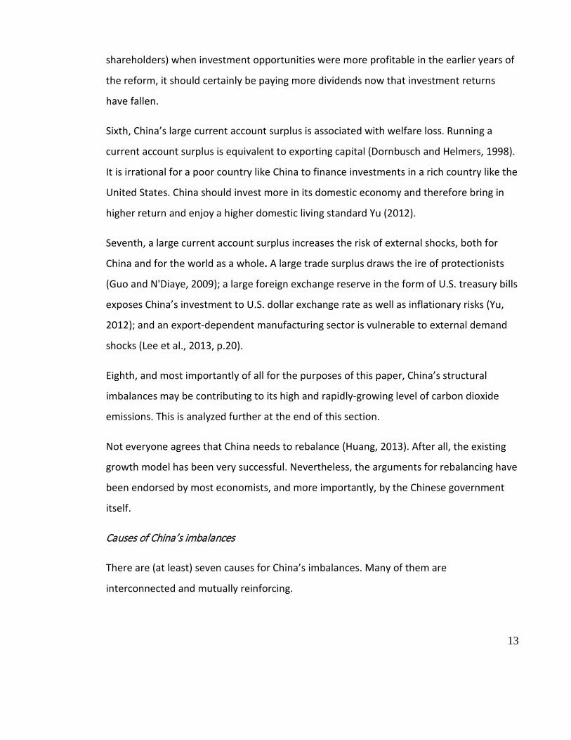
Sixth, China’s large current account surplus is associated with welfare loss. Running a

current account surplus is equivalent to exporting capital (Dornbusch and Helmers, 1998).

It is irrational for a poor country like China to finance investments in a rich country like the

United States. China should invest more in its domestic economy and therefore bring in

higher return and enjoy a higher domestic living standard Yu (2012).

Seventh, a large current account surplus increases the risk of external shocks, both for

China and for the world as a whole. A large trade surplus draws the ire of protectionists

(Guo and N'Diaye, 2009); a large foreign exchange reserve in the form of U.S. treasury bills

exposes China’s investment to U.S. dollar exchange rate as well as inflationary risks (Yu,

2012); and an export-dependent manufacturing sector is vulnerable to external demand

shocks (Lee et al., 2013, p.20).

Eighth, and most importantly of all for the purposes of this paper, China’s structural

imbalances may be contributing to its high and rapidly-growing level of carbon dioxide

emissions. This is analyzed further at the end of this section.

Not everyone agrees that China needs to rebalance (Huang, 2013). After all, the existing

growth model has been very successful. Nevertheless, the arguments for rebalancing have

been endorsed by most economists, and more importantly, by the Chinese government

itself.

Causes of China’s imbalances

There are (at least) seven causes for China’s imbalances. Many of them are

interconnected and mutually reinforcing.

13

The first and foremost is factor price repression. The cost of capital cost is depressed in

China (Huang and Wang, 2010a). China has one of the highest levels of financial

repression in the world (Dorn, 2006). Financial repression has been shown to be an

important driver of industrial expansion (Huang and Tao, 2010). There is also robust

evidence showing that, in combination with an export-promoting growth strategy,

financial repression constrains factors from moving to the service sector (Anders C and

Xun, 2011).

Labour wages are repressed too. China’s Household Registration System (HRS) prevents

migrant workers from receiving the health care, education and other social benefits as

their registered urban counterparts do. Migrant workers are willing to take lower wages

than registered urban workers for the same job (Huang and Wang, 2010a). Employers are

thus able to hire at low wages – this is especially true in the labor-intensive export sectors.

Resources prices are also repressed. Land prices are cheap due to state-ownership in the

cities and government’s ability to convert collectively owned farms into city lands at below

market prices (Wong, 2013) . The price of energy is low due to price regulation. The cost

of damage to the environment is not internalized because environmental regulations are

not adequately enforced.

These factor price depressions act as implicit subsidies for producers, investors and

exporters. Hence they are responsible for high investment, industrial production and

exports. And with depressed wage income, on which private consumption depends,

consumption is weak. Huang (2010) regards factor market distortions to be the

fundamental cause for China’s imbalances. It is estimated that the total producer subsidy

equivalents (PSEs) to be as high as 10.6 per cent of GDP and 9.6 per cent of the current

account balance in 2008 (Huang and Tao, 2010).

Yet there are other causes too.

14

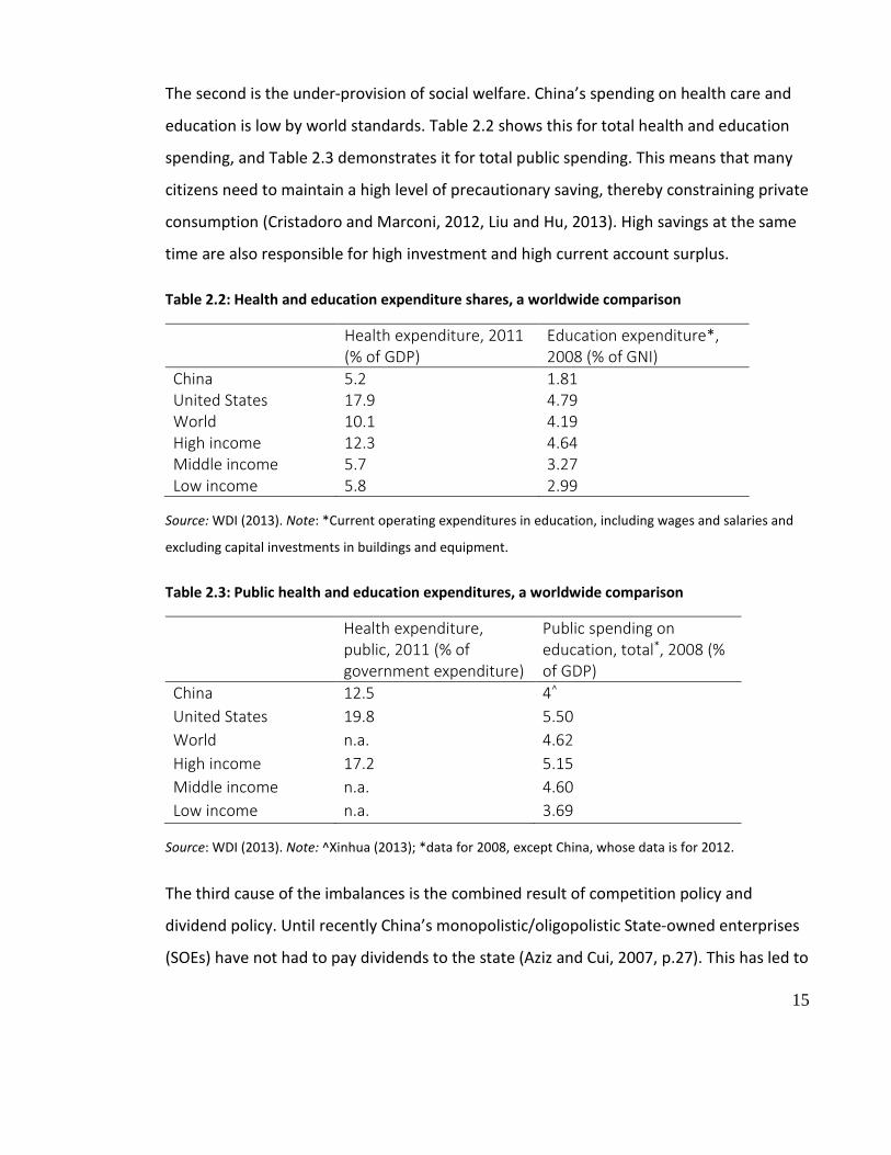
The second is the under-provision of social welfare. China’s spending on health care and

education is low by world standards. Table 2.2 shows this for total health and education

spending, and Table 2.3 demonstrates it for total public spending. This means that many

citizens need to maintain a high level of precautionary saving, thereby constraining private

consumption (Cristadoro and Marconi, 2012, Liu and Hu, 2013). High savings at the same

time are also responsible for high investment and high current account surplus.

Table 2.2: Health and education expenditure shares, a worldwide comparison

Health expenditure, 2011 (% of GDP)

Education expenditure*, 2008 (% of GNI)

China 5.2 1.81 United States 17.9 4.79 World 10.1 4.19 High income 12.3 4.64 Middle income 5.7 3.27 Low income 5.8 2.99

Source: WDI (2013). Note: *Current operating expenditures in education, including wages and salaries and

excluding capital investments in buildings and equipment.

Table 2.3: Public health and education expenditures, a worldwide comparison

Health expenditure, public, 2011 (% of government expenditure)

Public spending on education, total*, 2008 (% of GDP)

China 12.5 4^

United States 19.8 5.50 World n.a. 4.62 High income 17.2 5.15 Middle income n.a. 4.60 Low income n.a. 3.69

Source: WDI (2013). Note: ^Xinhua (2013); *data for 2008, except China, whose data is for 2012.

The third cause of the imbalances is the combined result of competition policy and

dividend policy. Until recently China’s monopolistic/oligopolistic State-owned enterprises

(SOEs) have not had to pay dividends to the state (Aziz and Cui, 2007, p.27). This has led to

15

a large saving-investment gap, which is ultimately responsible for the current account

surplus (Tyers and Lu, 2009). The strong savings at the same time also bolsters these

companies’ appetite for investment.

The fourth cause is the financial sector’s institutional setup. The finance sector is itself

dominated by the SOEs. State-owned banks prefer to lend to the SOEs. According to

Huang (2010, p.57), ‘the state sector accounts for only one-third of the Chinese economy,

but accounts for two-thirds of bank loans. SOEs also account for a dominant share of

funds raised from the market. This provides the SOEs yet stronger financial clout for

investment. SOEs also discriminate against smaller investors (Huang, 2010) and especially

the households. This limits households’ non-wage income and thus represses

consumption.

Fifth, international experience shows that high investment and a dominant industrial

sector go together. Figure 2.3 illustrates this point: there is clear positive relationship

between the share of industry and the share of investment in GDP for developing

countries, across time and income-groups. This can be explained by the fact that the

industry sector is more capital-intensive than either services or agriculture. And China’s

overinvestment problem is concentrated among the heavy-industry sectors, as discussed

in Section 2.

16

Figure 2.3: Relationship between investment and industry share in GDP, for different groups of countries between 1980 and 2010

Source: WDI (2013). Note: The data points are the averages for the different country groupings, in different

years.

Sixth, an undervalued currency contributes to the current account surplus (Huang and

Tao, 2010, Corden, 2009). Although the gradual appreciation of RMB since 2005 has

erased some of the surplus, it is projected (as of April 2012) that the surplus is likely to

rebound should real exchange rate remains unchanged (Cline, 2012).

Seventh, and last, the dominant industrial sector is export oriented, and this contributes

to the large current account surplus.

China’s future economic structure and reforms to reduce imbalances

One view is that China’s economic imbalances, though they have worsened in the past,

will reduce in the future, even without policy intervention (Huang, 2013). Particularly

important to this view is the concept of the Lewis Turning Point (LTP), the point at which

surplus labour vanishes. Reaching the LTP would drive up labour costs, increase wage

income, reduce China’s labour cost advantage and thus stimulate consumption, reduce

the trade surplus and promote the services sector.

15

20

25

30

35

40

10 15 20 25 30 35

Gro

ss c

apita

l for

mat

ion

(% o

f G

DP)

Industry, value added (% of GDP)

Low income

Middle income

High income

17

Another argument for this view is that per capita income and the importance of the

service sector are positively related (World Bank, 2004). Thus as China’s per capita income

rises, so too would the share of the service sector.

There are two main drivers for this. First, with regard to consumption patterns, as per

capita income increases, demand for agricultural and durable goods tend to saturate. At

the same time, demand for health care, travel and finance tend to increase (Wu, 2007).

With regard to the production process, as the diversification of workforce progresses,

firms increasingly rely on services in financing, legal practice, human resources,

technology, security and even management and strategy (ibid). This second factor is the

increasingly discussed process of “servicification” (Daniels and Ni, 2014). The literature

has also observed that the rate of service sector growth has a positive relationship with

democratization, openness to trade, proximity to financial centers and the level of

urbanization (Eichengreen and Gupta, 2013).

Demographic change can be another natural driver of structural change. China’s aging

population will require increasing volumes of age care, health care and social security

(Wagner, 2013).

How much and how quickly these “natural” economic factors will force rebalancing is an

open question. For example, till now the questions of whether China has crossed the LTP

and what the extent of the impact will be when it does actually crosses it are still not

settled (Yao and Zhang, 2010, Das and N'Diaye, 2013, Huang and Jiang, 2010, Wang,

2010).

In any case, Chinese policy makers are not sitting back and waiting for the economy to

adjust. Rather they are starting to take measures which attempt to address the causes of

the imbalances addressed previously. They have at least six to choose from.

18

First, giving a higher priority to welfare spending in the budget will increase the supply of

social welfare. The effect will be less precautionary saving and more consumption.

Following the first point, secondly, the HRS system needs to be reformed to allow migrant

and urban workers equal rights. The incremental income will be enjoyed by the migrant

workers, who, as lower-income-earners, tend to have higher propensities to consume.

Third, either through privatization or the establishment of a dividend-paying channel, the

savings from the SOEs should be made available to a wider population.

Fourth, removing financial repression would result in the interest rate rising. Assessing

borrowers on merit rather than ownership would reduce excessive investment.

Fifth, reducing energy subsidies and redirecting the budget towards tax cuts or welfare

spending could have a double effect on reducing heavy industry and boosting

consumption.

Sixth, the post-industrialization process can be accelerated by reducing the immobility of

the labour force (Lee and Wolpin, 2006). Programs such as targeted training and

education will help to prepare the labour force for the transition from the industry sector

to the service sector.

Chinese policy makers have committed to all of these in various policy papers and plans

and have started to implement most, though the jury is still out whether the extent of

implementation will be strong enough to make a change, and, more fundamentally,

whether the country’s political economy will support the radical policy changes needed.

China’s economic rebalancing and environmental challenges

China has the highest carbon dioxide emissions in the world and its emissions grow much

faster than the world average. As shown in Figure 2.4, China’s annual carbon dioxide

emissions increased from 1,425 million tons in 1981 to 8,000 million tons in 2011.

19

Between these years, China has outpaced the world in carbon dioxide emissions growth in

all but two years. As a result, its share of total global emissions went from 8 per cent up to

25.5 per cent.

Figure 2.4: China’s carbon dioxide emissions in a global context

Source: OECD iLibrary3 , author’s calculations.

Not only are China’s emissions high in absolute terms, they are also high in terms of

emissions per unit of GDP (see Figure 2.5). Although it has declined substantially since

1980s, the country’s carbon intensity of GDP is still one of the highest in the world. In fact,

among the 207 countries recorded in the World Bank dataset, only 9 had a higher carbon

intensity than China in 2010. The sudden drop in emissions intensity of LICs in 1997 visible

in Figure 2.5 illustrates China’s high emissions intensity and its high share of global

emissions – 1997 was the year in which China graduated from the LIC group to join the

MIC group.

3 Data extracted on 16 Nov 2013 17:55 UTC (GMT) from OECD iLibrary.

-0.05

0

0.05

0.1

0.15

0.2

0.25

0.3

0

1000

2000

3000

4000

5000

6000

7000

8000

9000

1981 1983 1985 1987 1989 1991 1993 1995 1997 1999 2001 2003 2005 2007 2009 2011

China CO2, mt (L-axis) World CO2 growth %, p.a. (R-axis)

China CO2 (% of World) (R-axis) China CO2 growth %, p.a. (R-axis)

20

Figure 2.5: Carbon emissions intensity of GDP, China in the world

Source: WDI (2013). Note: CHN, HIC, MIC and WLD denote China, high-income-country, middle-income-

country and world, respectively.

There are four closely related reasons as to why China’s emissions are high, both in

absolute and intensity terms. First, the share of the industry sector is high and industry is

more carbon-intensive than services. Several studies have found that the increase of the

I/S ratio in the early 2000s in China led to the increase in carbon intensity over the same

period (Wu, 2011, p.706, Chen, 2011). Li (2011a) identified that structural shifts between

sectors were the driving factor behind the upward trend in energy intensity between 2001

and 2005.

Second, within the industry sector, the share of the most energy- and carbon-intensive

heavy–industry sectors has grown faster. Figure 2.6 shows that around year 2002 the ratio

of heavy to light industry started to rise, and that the economy’s emissions intensity

ended its rapid decline, resulting in much more rapid growth in emissions.

00.5

11.5

22.5

3

kg per 2005 PPP $ of GDP

CHN HIC LIC WLD

21

Figure 2.6: Emissions intensity and heavy industry

Source: WDI (2013).

Due to the strong demand from the industry sector and especially the heavy-industry

sector, China is highly dependent on energy. China’s energy intensity of GDP in 2010 was

significantly higher than the world average, the Europe Union’s average and the United

States’ (see Table 2.4). In fact, it was even higher than the oil-rich Arab World average.

Table 2.4: Energy intensity and fossil fuel dependency, a worldwide comparison, 2010

Energy use (kg of oil equivalent) per $1,000 GDP (constant 2005 PPP)

Fossil fuel energy consumption (% of total)

China 265 88 United States 170 84 World 181 81 European Union 123 75 Arab World 213 97 Russian Federation 348 91

Sources: WDI (2013).

Third, to make matters worse, China’s energy is highly dependent on fossil fuels. Again, by

Table 2.4, fossil fuels contribute to 88 per cent of China’s total energy consumption. This

0.00E+00

1.00E+06

2.00E+06

3.00E+06

4.00E+06

5.00E+06

6.00E+06

7.00E+06

8.00E+06

9.00E+06

0

1

2

3

4

5

6

1980

1982

1984

1986

1988

1990

1992

1994

1996

1998

2000

2002

2004

2006

2008

2010

CO2 emissions (kg per PPP$ of GDP), L-axis

Heavy/Light ratio, L-axis

CO2 emissions (kt), R-axis

22

was higher than the world average and also larger than the United States’. In fact it was

not much lower than the fossil-rich Russia.

Given the link between industrial dominance and carbon dioxide emissions, we expect

that a structural rebalancing towards less investment and industry and more consumption

and services would help China’s transition towards a low-energy, low-carbon economy.

The aim of this chapter is to provide a quantitative analysis of this transition, and an

estimate of the likely impact of the former on the latter.

2.3 Modelling the link between rebalancing and emissions: literature survey

and approach

Literature survey

Despite the clear links between rebalancing and emissions, there are only a few studies

which have explored the subject (e.g., McKay and Song, 2010, Howes and Dobes, 2010).

Even fewer have undertaken forward-looking quantitative analysis in a rigorous manner.

Feng et al. (2009)’s regression analysis showed that between 1980 and 2006, a 1

percentage point increase in the share of service sector value added in GDP led to 0.6 per

cent decrease in energy intensity in any given year. Howes (2012) used a simple back-of-

the-envelope calculation to suggest that a 10 per cent switch in the GDP composition from

industry to service will lead to 14 per cent reduction in energy intensity. Neither set of

calculations is based on estimating emissions in a restructured economy, in which both

service-industry and investment-consumption ratios would be very different to their

current levels.

Indeed, there are very few efforts to model China’s rebalancing even without

consideration of the implications for emissions. He and Kuijs (2007) is a rare exception.

Theirs is an influential study, providing the underpinning for the modelled results in the

23

well-known China 2030 report (World Bank and the Development Research Center of the

State Council, 2013).

He and Kuijs use the DRC-CGE model, a computable general equilibrium model developed

by the Development Research Centre of China. They shock a number of parameters to

quantify the impact of rebalancing. In their two growth scenarios, GDP growth is the

same, but the investment and industry shares of GDP are different. A significant reduction

in investment’s share in GDP is projected – almost halving its share compared to a past-

trend scenario to an average of 28 per cent of GDP between 2025 and 2035. A smaller but

still significant reduction in the share of industry in GDP is projected. It falls from 51 per

cent of GDP to 36 per cent, by 2035.

The aim of this chapter is to understand the emissions implications of the sort of

rebalancing which He and Kuijs model, and which the China 2030 report highlights. The

basic question it seeks to answer is: how would China’s emissions be affected by economic

rebalancing? To do this, we need a rebalancing and a baseline scenario, a model, and a

modelling procedure. These are presented in the next three sub-sections.

Baseline and rebalancing scenarios

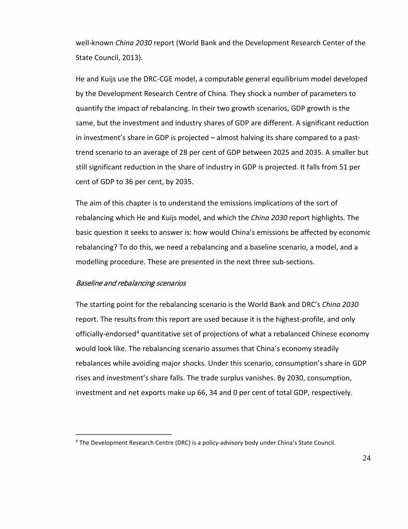
The starting point for the rebalancing scenario is the World Bank and DRC’s China 2030

report. The results from this report are used because it is the highest-profile, and only

officially-endorsed4 quantitative set of projections of what a rebalanced Chinese economy

would look like. The rebalancing scenario assumes that China’s economy steadily

rebalances while avoiding major shocks. Under this scenario, consumption’s share in GDP

rises and investment’s share falls. The trade surplus vanishes. By 2030, consumption,

investment and net exports make up 66, 34 and 0 per cent of total GDP, respectively.

4 The Development Research Centre (DRC) is a policy-advisory body under China’s State Council.

24

With regard to sectoral composition, the China 2030 rebalancing scenario projects that by

2030, agriculture, industry and services will account for 4, 35 and 61 per cent of GDP,

respectively. This particular result requires the share of the agriculture sector to fall by

more than 50 per cent, and, according to our simulations, is unrealistically large. In this

case, therefore, we adjust the China 2030 rebalancing scenario to keep the share of

agriculture the same as it was in 2013. We focus solely on rebalancing from industry to

services. Hence in our rebalancing scenario by 2030 the shares of the primary, secondary

and tertiary sectors are 10, 35 and 45 per cent of GDP, respectively. Given that the

primary sector is the least emissions-intensive among the three (see Table 2.10 in Section

2.4), if its share falls in the future – which is likely to be the case, we could overestimate

structural rebalancing’s contribution to emissions reductions. That said, it is reasonable to

believe the fall in primary sector will be matched by a one-for-one increase in service

sector share, as the difference in emisisons intensity between these two sectors is

relatively small, the extent of the overestimation is also likely to be small.

Average real GDP and population growth over the period are assumed to be 6.2 per cent

and 0.16 per cent, respectively. Table 2.5 summarises these assumptions.

One limitation of the World Bank and DRC (2013) study is that it lacks a baseline. For

meaningful quantitative comparisons, we need a baseline with which we can compare our

rebalancing scenario.

He and Kuijs (2007), on which the China 2030 report was based, take as their baseline an

extrapolation of past trends. Thus in their baseline investment and industry shares

continue to rise. This is implausible. Section 2 highlighted a number of reasons why, even

without significant policy change, some rebalancing might take place. We take as our

baseline the maintenance of current shares. Thus the assumption is that the current

extent of imbalance remains, rather than that the imbalances further worsen.

25

As with He and Kuijs (2007) and the World Bank and DRC (2013), we assume that

rebalancing does not affect real GDP. Having real GDP growing at the same rate between

the baseline and the policy case also allows us to focus purely on shifts in the way output

is produced, rather than on changes to the level of output, when it comes to thinking

about emissions. Table 2.5 puts the two scenarios side by side.

Table 2.5: Baseline and policy scenario economic structures, 2030

Baseline (status quo) Policy (rebalancing) Real annual GDP growth Real GDP growth 6.2% p.a. Labour growth 0.2% p.a. GDP Expenditures Share of GDP

C 50% 66% I 46% 34%

Industries Share of industrial value-added AGR 10% 10% IND 45% 35% SRV 45% 55%

Source: World Bank and DRC (2013), WDI (2013) for real GDP and labour growth rates.

CGE Model

A recursive dynamic computable general equilibrium (CGE) model, CHINAGEM, is

employed to conduct the simulation. It is a single country, top-down model. The core

theories of the model are based on the MONASH model (Dixon and Rimmer, 2007). An

emissions accounting framework and an energy accounting framework are incorporated

into CHINAGEM as is done in the MMRF model (Adams and Parmenter, 2013). A

documentation of CHINAGEM can be found in Mai et al. (2010). The model uses the 2002

Chinese Input-Output table as the main database. For the current study, the economic

structure is updated to represent the structure of the economy in 2012.

Simulation method

26

The approach we use is to allow a small number of economic parameters, normally held

constant, to vary so that the desired economic shares and growth rates are achieved. We

have six target variables: the rate of GDP growth, two shares of GDP - total consumption

and investment; and three shares of sectoral value added – agriculture, industry and

services. To achieve these six targets, we make the following six (normally exogenous)

parameters to be endogenous: general factor productivity; the average propensity to

consume in GNP; the return to capital; and the demand for agricultural, industrial and

service inputs. Table 2.6 outlines these closure choices.

Table 2.6: Closure for both the baseline and policy scenario

Exogenenized Endogenized Real GDP growth General factor productivity: GFP

Nominal consumption share in GDP Average propensity to consume in GNP: APC

Nominal investment share in GDP Expected rate of return to capital: EROR

Agriculture sector share in total VA Input-demand shifter: agriculture sector: IDS(agr)

Industry sector share in total VA Input-demand shifter: industry sector: IDS(ind)

Service sector share in total VA Input-demand shifter: service sector: IDS(srv)

Source: Author’s assumptions.

Clearly, rebalancing requires that the propensity to consume rises. Likewise, it requires a

higher return on capital, to end financial repression and over-investment. Less investment

will, on its own, mean lower growth, but we would expect factor productivity to be higher

as a result of rebalancing reforms, which enables growth to be kept constant across the

two scenarios.

We do not distinguish between private and government consumption, but we fix the

budget deficit to nominal GDP ratio across scenarios to ensure fiscal sustainability.

27

In terms of sectoral composition, we endogenise the three sectoral “input-demand

shifters” to model the “servicification” of the economy. These allow cost-neutral5 shifts in

the demand for intermediate goods produced by each of the three broad sectors. The

expectation is that rebalancing increases the demand for services and reduces it for

industry.

Additionally, the nominal exchange rate of the RMB is chosen as the numeraire; and the

world price level is also assumed to be fixed.

Regarding the modelling technique, a two-stage procedure is required. If we shock all

three of the shares of agriculture, industry and services at the same time, the model tends

not to solve.6 But if we only shock two of these three, one of the sectoral demand-shifters

has to be chosen to be exogenous. Preliminary tests show that the choices made here can

lead to inconsistent solutions.7

To get around this problem, we use a two-stage approach. In the first stage, for each

scenario, only three variables are targeted: GDP growth, the consumption share and the

investment share. Nominal sectoral value added is thereby obtained for each scenario,

and used, along with information on target shares, to calculate nominal growth rates for

industry, agriculture and services value added. These are then used as targets in a second

simulation, along with the investment and consumption shares already used, as well as

the real GDP and labour growth rates.

5 The cost-neutral condition ensures that a fall/increase in input use by a producer/investor is matched by a comparable increase/fall in output, such that that the unit costs of production/investment remain the same. 6 This is both because the model is solved by linear approximation and because externally calculating the rates of change in sector shares inevitably creates rounding errors. Since when the rate of changes in the three shares are shocked, the sum of the shares of all sector’s value-added must add to exactly 1, this becomes an unrealistic demand for the model to cope with. 7 For example, endogenizing the input demand shifters for agriculture and industry leads to different results comparing with endogenizing the input demand shifters for industry and services.

28

This two stage procedure ensures that the model solves, and gives the target sectoral as

well as demand-side shares desired.

2.4 Simulation results

In this section we show the cumulative, percentage deviations8 in the policy (rebalancing)

scenario relative to baseline (status-quo). The results should be read as the overall impact

of the rebalancing policies over the 18 years between 2013 and 2030.

The macro-economy

Real GDP income is unchanged by assumption. Table 2.7 shows the simulation results on

the income side of GDP. General factor productivity improves9 as expected: with lower

investment, the economy needs higher factor productivity to maintain rapid growth.

Capital employment falls due to the reduced investment. Labour hours also fall as a result

of the higher general factor productivity, so that less labour input is needed. As

capital/labour ratio decreases, marginal productivity of capital increases relative to

marginal productivity of labour.

Table 2.7: GDP and factor growth, cumulative percentage deviation by 2030

Real GDP 0 General factor productivity 8 Capital -11 Producers’ unit capital cost 57 Labour hours -1 Producers’ unit labour cost 5

Source: CHINAGEM, author’s simulations.

The composition of GDP changes due to the rebalancing, as Table 2.8 shows. (Demand-

side shares under the two scenarios have already been shown in Table 2.5.) Real

8 Unless otherwise stated. 9 The general factor productivity shifter being negative represents an improvement in factor productivity.

29

consumption increases by 46 per cent, due to the increase in the average propensity to

consume.

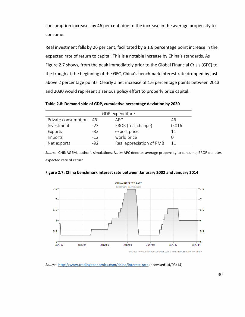
Real investment falls by 26 per cent, facilitated by a 1.6 percentage point increase in the

expected rate of return to capital. This is a notable increase by China’s standards. As

Figure 2.7 shows, from the peak immediately prior to the Global Financial Crisis (GFC) to

the trough at the beginning of the GFC, China’s benchmark interest rate dropped by just

above 2 percentage points. Clearly a net increase of 1.6 percentage points between 2013

and 2030 would represent a serious policy effort to properly price capital.

Table 2.8: Demand side of GDP, cumulative percentage deviation by 2030

GDP expenditure Private consumption 46 APC 46 Investment -23 EROR (real change) 0.016 Exports -33 export price 11 Imports -12 world price 0 Net exports -92 Real appreciation of RMB 11

Source: CHINAGEM, author’s simulations. Note: APC denotes average propensity to consume, EROR denotes

expected rate of return.

Figure 2.7: China benchmark interest rate between Janurary 2002 and January 2014

Source: http://www.tradingeconomics.com/china/interest-rate (accessed 14/03/14).

30

Net exports (exports minus imports) almost vanish as exports fall by more than imports

(both fall as the industrial sector shrinks, but imports are somewhat protected by the

increase in consumption). This requires a fall in the competitiveness of China’s goods and

services. World prices are assumed to be constant with the nominal exchange rate being

fixed. Thus the loss in global competitiveness can only come from an increase in the

domestic price level, i.e., a real appreciation of the RMB. This in turn pushes up China’s

export price index. Real exports hence fall by 33 per cent.

The real appreciation of the RMB should increase imports, but imports in fact fall by 12

per cent. This is because the majority of China’s imports are used as intermediate inputs in

the manufacturing (part of the industry sector) sector. Import demand falls when the

manufacturing sector shrinks – which the next subsection illustrates. Though China’s fall in

exports could lead to a rise in production, and thus emissions, from other countries, a fall

in real input demand from China is added good news to global mitigation as it could lead

to carbon savings elsewhere in the world.

Sectoral results

Overall sector results are summarised in Table 2.9. The agriculture and industry sectors

produce 4 per cent and 15 per cent less output, respectively. The service sector produces

19 per cent more. These changes are driven by the input-demand shifts in the respective

sectors. The rise in the input-demand shifter for services, and the falls for agriculture and

industry represent the “servicification” of the Chinese economy.

Table 2.9: Sector output, prices and input demand, cumulative percentage deviation by 2030

Source: CHINAGEM, author’s simulations.

output Price Input-demand shifter

Agriculture -4 10 -57 Industry -15 2 -16 Service 19 9 20

31

The directions of output changes are the same as the input demand shifts for all three

sectors. This is reasonable since the input-demand shifters are cost-neutral – a reduction

(or increase) in inputs used by a sector will lead to a comparable reduction (or increase) in

its outputs. This effect dominates in the industry and service sectors. For the agriculture

sector, however, a significant fall in input-demand only leads to a small fall in output. Two

factors are responsible for this. First, the agriculture sector sells a relatively larger

proportion of its outputs as consumer goods to the households. Thus the rise in

consumption in the rebalancing scenario raises the final demand for agriculture goods.

Second, the agriculture sector is relatively more labor-intensive than the other two

sectors. Thus as capital becomes relatively more expensive than labour in the rebalancing

scenario this supports the production of agriculture outputs. Hence these two effects

together partially offsets the big fall in input demand for agriculture outputs.

The price level of all three sectors increases in line with the general increase in domestic

price level as discussed earlier.

We look at the sectoral results, in particular those that are related with emissions, in more

detail in the next subsection.

Emissions

Simulation results shown in Table 2.10 show that the structural rebalancing will lead to a

17 per cent reduction in carbon dioxide emissions. Given that real GDP is constant, the

emissions intensity of GDP also falls by 17 per cent. Table 2.10 also records the emissions

and emissions intensity for the industry and service sectors in 2030, under both scenarios.

32

Table 2.10: Sectoral value-added, carbon dioxide emissions and emissions intensity index, 2030

2030 VA share Carbon emissions share

Carbon-intensity index

Base Agriculture 10% 1% 0.3 Industry 45% 79% 5.7 Services 45% 21% 1.5

Policy Agriculture 10% 1% 0.2 Industry 35% 74% 5.1 Services 55% 25% 1.1

Source: CHINAGEM, author’s simulations.

Two factors contribute to the fall in emissions intensity. First, the share of the industry

sector, which is far more emissions intensive, decreases relative to the share of the service

sector. This is the contribution from sectoral rebalancing we expected.

Second, not only do the shares of emission-intensive activities fall, but the emissions

intensities across all sectors are also lower in the rebalancing scenario than in the status

quo (see

33

Table 2.10). This effect has been overlooked in previous studies, but is an important

outcome of the “servicification” of the economy, which results in the economy in general

using less industrial output in both production and investment.

Our findings show a stronger emission reduction in emissions intensity than the literature.

The regression analysis of Feng et al. (2009) shows that one per cent increase in service

sector share led to 0.6 per cent reduction in energy intensity between 1980 and 2006. If

such a relationship is preserved, a 10 per cent switch between the shares of industry and

services implies a reduction of energy intensity of 11 per cent over the 18 years between

2013 and 2030. Howes (2012) predicts that increasing service sector share by 10 per cent

of GDP and reducing industry sector share by the same amount would reduce energy

intensity by 14 per cent.

The Howes study assumed constant energy intensities within each broad sector, and took

no account of a changing demand side, or of increased productivity, or reliance on service-

sector inputs across the economy. The current study shows that emissions intensity will be

lower across all sectors – implying an underestimation of emission reduction by Howes

(2012).

Howes (2012) also assumes that the entire change in the composition of sectoral value

added is achieved by changes in real output. This study shows, however, that price

changes also contribute to the change in sectoral value-added shares. The fact that the

industry price level increases suggests industry output falls more than expected – implying

again an underestimation of emission reduction by Howes (2012).

2.5 Concluding remarks

China needs to rebalance its economic structure from a focus on investment and exports

to one on consumption and services. Since the current economic structure is energy- and

34

emission-intensive, rebalancing the economic structure has the potential to reduce the

country’s emissions.

This paper tries to quantify the contribution of China’s structural rebalancing to its

emissions reduction. The paper devises two scenarios. Under one, the Chinese economy

preserves its current structure and, under the other, it successfully rebalances it. A two-

stage simulation method is used to carry out the simulation, allowing a few key

parameters to adjust endogenously. The results show that between 2013 and 2030,

successful rebalancing will help the country to reduce its emissions by 17 per cent. This is

higher than the two existing, partial-equilibrium estimates.

More rigorous analysis conducted here has unearthed additional general-equilibrium

mechanisms by which rebalancing will reduce emissions. The reason for our estimations to

be higher than previous results are these general equilibrium effects. On the one hand

rebalancing reduces emissions intensity across all three aggregated production sectors; on

the other hand changes in price levels require industry output to fall more than expected

and service output to rise less.

The focus has been on the transition from industry to services. This is consistent with the

agricultural share being held constant. This might result is a overestimation of the

emissions reduction since the emissions intensity of agriculture is lower than that of

services, and it is likely that the agricultural share will continue to fall over time. However,

any such overestimation will be small due to the relatively small difference in emissions

intensity between agriculture and services, and the small share of agriculture to begin

with.

Although our modelling is a significant advance on earlier efforts, there are still short-

comings, and the results we have obtained remain, while illuminating, indicative only. We

have no way, for example, to capture the relationship between SOE reform and its

35

potential contribution to increasing the cost of capital, nor is there any allowance for

greater investments in education to accelerate the “servicification” process.

Nevertheless, it is clear from our results that economic rebalancing holds non-negligible

abatement potential. This is not only another reason to rebalance the Chinese economy. It

is also a justification for the use of ambitious mitigation targets, at least in the short-run

where emissions savings can be made not only by the adoption of environmental

instruments and regulations but by the pursuit of economic reform.

36

Chapter 3 Efficiency improvements in coal-fired

power generation and emissions reduction

Abstract

Coal-fired power generation efficiency has been an important driver of energy and

emissions intensity in China, and over the last decade improvements in the former have

significantly reduced the latter. This study argues, however, that in the coming years

further efficiency improvements in coal-fired power plants will make a still important but

much more modest contribution to achieving China’s emissions targets. Between 2005

and 2012, coal-fired power plant efficiency improved by an average of 1.84 per cent a

year, contributing approximately a reduction of 5.8 percentage points in emissions

intensity or 24 per cent of the overall reduction in emissions intensity achieved over this

period. Between 2012 and 2020, we project that coal-fired power plant efficiency will

improve by 0.91 to 0.97 per cent a year, contributing approximately a reduction by 2020

of 2.5 to 3.0 percentage points in emissions intensity, or 9 to 11 per cent of the required

reduction to achieve China’s 2020 emissions intensity target. This approximate halving in

the pace and importance of improvements in coal-fired power generation efficiency is for

two reasons. First, and most importantly, after the progress already made, China’s current

coal-fired power generation efficiency is already close to global best practice. Second, the

scope for building new coal-fired power plants is being squeezed by renewable energy and

structural rebalancing. The essay shows that, going forward, switching to renewable

energy and structural rebalancing will be more important for achieving China’s emissions

targets than improving coal-fired power generation efficiency. That said, improvements in

coal-use efficiency will still be needed. To fully achieve China’s emissions intensity

37

reduction target, a combination of all three – structural rebalancing, renewable energy

promotion, and coal-use efficiency improvement – will be needed.

3.1 Introduction

China’s coal-fired power generation is a major contributor to global carbon dioxide

emissions. China released 8,206 million tons of carbon dioxide from the combustion of

fossil fuel in 2012, 26 per cent of the world’s total (IEA, 2015). The electricity sector alone

contributed 4,050 million tons – 49 per cent of China’s total emissions (ibid). And coal-

fired power plants produced almost all of the emissions of the electricity sector – 3,984

million tons (ibid) – or 48 per cent of China’s total emissions. Thus China’s coal-fired

power plants accounted for about one eighth of the total carbon emissions from fuel

combustion in the world in 2012.

Such sheer scale means a small efficiency improvement in China’s coal-fired power plants

could lead to a large fall in carbon emissions. If coal-using efficiency in China’s power

plants increases by 1 per cent, everything else being equal, the country’s overall emissions

would fall by 0.49 per cent, and global emissions by 0.13 per cent.

Since just before the turn of the century, China has been trying to improve the efficiency

of its coal-fired power plants. China initiated plans to phase out small and inefficient (SAI)

thermal power plants in the late 1990s. Units with a capacity below 50 megawatts (MW)

were scheduled to be closed down by 2003 (State Economic and Trade Commission,

1999). And China’s 10th Five Year Plan (FYP) scheduled the retirement of a total of 15

gigawatt (GW) of SAI capacity between 2001 and 2005.

However, a surge in industrial and investment demand disrupted these plans. Accelerated

economic growth combined with a boom in the energy-intensive parts of the economy led

to a power-shortage from 2002 onwards (Shen, 2004). As a result, many SAI units were

retained rather than closed. By the end of 2005, only 8.3GW had been closed and only

38

about half of China’s fleet were large power plants, with a capacity above 300MW (Zhang,

2007).

The improvement in overall coal-fired power generation efficiency was relatively slow

between 2003 and 2006. The average amount of coal used to supply one kWh electricity

to the grid was 380 grams of standard coal (gsc) in 2003, when data were first available.

This fell to 367 gsc per kWh in 2006, an average reduction of 1.15 per cent per annum

(Figure 3.1).

Figure 3.1: Coal-fired power plants efficiency: standard coal per kilowatt-hour electricity supply to the grid†

Source: China Electricity Council (2014). Note: Data for year 2011 and 2012 are for plants of capacities above

6000kW, whereas data for all previous years are for plants of all capacities. Hence data for 2010 and 2011

may slightly overstate the rate of improvement of coal-use efficiency in power generation.

Then in early 2007, in the wake of acute environmental challenges and a recognition of

the need to transform the growth model, the closure of SAI units was once again

emphasized. China’s 11th FYP targeted the closure of 50GW of SAI capacity between 2006

and 2010. One key new policy was the Large Substitute Small (LLS) campaign that

320

330

340

350

360

370

380

390

2003 2004 2005 2006 2007 2008 2009 2010 2011 2012

gsc/kWh

39

mandated old SAI capacity (below 50MW) to be replaced by new, larger and more

efficient plants (above 300MW).

The new campaign was more successful. By 2010, 76.8GW of SAI capacity had been

replaced by more efficient capacity and 70 per cent of China’s power generating fleet was

above 300 MW. Unit coal use in power generation fell to 325gsc/kWh in 2012 – an

average reduction of 1.84 per cent per annum from 2005 (Figure 3.1).

This period also saw a faster improvement in overall energy and carbon efficiency. Figure

3.2 shows index values for the carbon emissions intensity of GDP, energy intensity of GDP

and coal-fired power generation efficiency in China between 2003 and 2012. By 2012, the

three variables are respectively 81, 83 and 86 per cent of their 2003 values, with the most

rapid decline in all three variables coming after 2006.

Figure 3.2: Carbon intensity, energy intensity and coal-fired power generation efficiency in China

Sources: Carbon and energy intensity: IEA (2015); coal-using power generation efficiency: China Elecpower

Year Book, various years. Note: All indexes are normalized to be 1 in 2003.

0.70

0.75

0.80

0.85

0.90

0.95

1.00

1.05

1.10

2003 2004 2005 2006 2007 2008 2009 2010 2011 2012

CO2 / GDP PPP (kgCO2 per 2005 USD)

TPES / GDP PPP (MJ per 2005 USD)

gsc/kWh

40

It is the consensus of the literature that efficiency improvement has been the most

important factor in reducing China’s energy intensity since 1980 (Ma and Stern, 2008;

Chen, 2011; Li, 2011). Ma and Stern (2008) show that within-sector changes in energy

efficiency have traditionally been the dominant factor, either upwards or downwards,

behind changes in energy intensity in China.

Li (2011) disaggregates the sectoral contributions to technical efficiency and estimates

that thermal power generation made the biggest contribution to improving technical

efficiency in China between 2000 and 2008. According to Li (2011), the thermal power

sector contributed to energy savings of nearly 50 million tons of coal equivalent (mtce)

between 2006 and 2008. This was the largest among all sectors. In comparison, the

second to fourth ranked sectors, namely steel, cement, paper and cardboard and coal,

respectively, each contributed between 10 and 20 mtce. No other sector contributed

more than 5 mtce.

Our analysis confirms the importance of improvements in coal-fired power efficiency.

Between 2005 and 2012 coal-fired power plant efficiency improved by 12.2 per cent. That

was a contribution of approximately 5.8 percentage points (12.2 times 0.48), or 24 per

cent (5.8 divided by 24) of the 24 per cent overall reduction in emissions intensity over the

same period.

However it would be naïve to simply extrapolate such trends into the future. Efficiency

improvement in coal-fired power generation is more difficult as the technological frontier

is approached. Moreover, as growth slows down and the structure of the economy

becomes less energy-intensive, the space for adding new capacities will also shrink. No

study has projected the potential contribution of efficiency improvement in coal-fired

power generation to emissions intensity in the future. This chapter attempts to fill that

gap.

41

The aim of this chapter therefore is to estimate the potential for further improvement in

coal-fired power generation efficiency in China, and to analyse the impact of any such

improvement on reducing the emissions intensity of GDP. Section 2 develops a method for

projecting potential gains in coal-fired power generation efficiency by 2020. Section 3

introduces the CGE model this chapter deploys, and uses it to estimate base case

emissions as well as demand for coal-fired power generation in 2020. Section 4 then uses

both the CGE model and our coal-use efficiency projection method to estimate the

contribution of coal-fired power generation efficiency improvement to the reduction of

emissions intensity of GDP. It shows that in fact the contribution of coal-use efficiency

improvement is a relatively minor one, and not enough to get China close to its emissions

targets. Section 5 looks at alternative scenarios involving rebalancing and renewable

energy, which have the side-effect of giving coal efficiency improvements an even smaller

role, but which, more importantly, will help China to hit its emissions targets. Section 6

concludes.

3.2 A method to project China’s coal-fired efficiency improvement

If the rate of efficiency improvement between 2012 and 2020 followed the trend between

2005 and 2012, unit output coal use would fall at 1.84 per cent per year, or by a total of

13.8 per cent over the 8 years, reaching an average of 280gsc/kWh in 2020.

However, it is unreasonable to simply extrapolate past trends like this, since such

performance would likely imply China expanding the global technological frontier. The IEA

(2011) projects that the highest possible average efficiency in coal-fired power plants in

advanced economies will reach 288gsc/kWh by 2020. It is not plausible to argue that

China could do better than this.

On the other hand, China’s stated targets underestimate where it could end up. The 12th

Five Year Plan sets the target for the national average coal-fired power generation

42

efficiency in 2020 to be 315gsc/kWh. This is far less efficient than either best practice or

the past trends would suggest.

What then is a reasonable target to aim at, within the range of 315 gsc/kWh (too

conservative) and 280 gsc/kW (too ambitious)? To answer this question, we need first to

look at the current coal-fired power generation fleet, and then to project its evolution.

Table 3.1 shows the composition of the current fleet, as of 2010, the most recent year for

which this data is available. Given that the LSS campaign sets 300MW as the minimum

capacity required of new plants, we categorize units with capacities below 300MW as SAI.

Table 3.1: Composition of China’s coal-fired power generation fleet, 2010

Unit capacity (MW)

Efficiency classification

Total capacity (MW)

Capacity share

Heat rate (gsc/kWh)

1000 non-SAI 33000 0.048 286 600 non-SAI 222470 0.321 292 [300-600) non-SAI 248570 0.358 334 [200-300) SAI 52010 0.075 350

[100-200) SAI 60720 0.088 380 [6-100) SAI 76720 0.111 420

Total weighted average efficiency :333

Average non-SAI efficiency: 312 Average SAI efficiency: 388

Sources: Productivity Commission (2011) for efficiency, China Electricity Council (2011), p49, Table 5-3 for

capacity shares. Note: Units of capacities below 6MW are not included.

In 2010, 73 per cent of the units were non-SAI. The average efficiency of the non-SAI and

SAI units were 312gsc/kWh and 388gsc/kWh respectively, and the overall efficiency of the

fleet was 333gsc/kWh.

To project the average efficiency of coal-fired power generation by 2020 we need to make

a number of assumptions of how the composition of the fleet will evolve. First, we

aggregate all the new coal-fired power plants commissioned in 2011 and 2012, the last

year for which such data are available. These projects are published on the National

43

Development and Research Commission (NDRC) website. The website also includes the

technology types of most of these projects. In Table 3.2, we match the new capacities with

the efficiencies shown in Table 3.1, according to their unit sizes and technology types. The

average efficiency of these newly-commissioned plants is 298gsc/kWh.

Table 3.2: NDRC commissioned new coal-fired power plants in 2011 and 2012

Unit capacity (MW)

Technology Type

Total capacity (MW)

Capacity shares

Heat rate (gsc/kWh)

1000 USC 8000 34% 286 600 USC 2400 10% 292 SupC 600 3% 299 SubC 1200 5% 310 Unspecified 1200 5% 299 350 SupC 3850 16% 299 Unspecified 700 3% 310 300 SupC 300 1% 299 Unspecified 5100 21% 310 200 Unspecified 400 2% 330

Sources: NDRC (2012), Productivity Commission (2011). Notes: Ultra-supercritical (USC); Supercritical (SupC);

Subcritical (SubC). The total capacity of the new (2011 and 2012) plants published on the NDRC website was

19.85GW.

Second, we assume the average efficiency of all the new plants installed during the 12th

FYP and the 13th FYP to be 298gsc/kWh and 288 gsc/kWh, respectively. This is consistent

with China’s target that the average efficiency of the new plants should be lower than

300gsc/kWh (NDRC, 2014), and is also consistent with findings for 2011 and 2012, and has

plant introduced between 2015 and 2020 at the global technological frontier of 288

gsc/kWh.

Third, we assume that by 2020, all the SAI plants will be phased out.

Fourth, we assume that the average efficiency of all retained plants will improve slightly

from 312gsc/kWh in 2010 to 310gsc/kWh by 2020. The latter is the stated target of the

44

Coal-fired Power Generation Energy Saving and Emissions Mitigation Upgrading and

Transformation Action Plan (NDRC, 2014). All new plants introduced since 2010 are

assumed to be still operating in 2020 at their nameplate level of efficiency.

Fifth, we assume that new plants are introduced into the fleet by 2012 and 2020 to (a)

compensate for the withdrawn SAI capacity and (b) increase total capacity in line with the

projected increase in coal-fired power generation under the base case.

These assumptions give us a method for projecting China’s potential coal-use efficiency

improvements. To develop projections for 2020, we need estimates for electricity demand

in that year, a task which the next section takes forward.

3.3 The CGE model, generic assumptions and the base case scenario

The model used is the CHINAGEM model (Mai et al., 2012). The version used in Chapter

Two is enhanced by distinguishing between six types of power generation sectors by

fuel,10 namely coal, oil, gas, nuclear, hydro-electricity and other.

The macroeconomic assumptions deployed follow those in Chapter 2. Real GDP is

assumed to grow at 7 per cent per annum, and labour employment at 0.36 percent per

annum between 2012 and 2020.11 Capital growth is driven by investment, which in turn

depends on the rates of return. As in Chapter 2, a general-factor-productivity variable is

endogenized to allow real GDP to grow at the assumed rate, the nominal currency

exchange rate is the numeraire, and world prices are assumed constant.

10 This change was made by Mark Horridge at the Centre of Policy Studies, Victoria University. 11 The assumptions are consistent between those made in Chapter Two, where real GDP is assumed to grow at 6.2 per cent per annum and employment at 0.2 per cent per annum, between 2012 and 2030. The higher rates assumed for 2012-2020 reflect the common belief that China’s real GDP and employment growth rates will slow over time.

45

Because in the course of chapter we want to isolate the impact of all three of (i) coal-fired

power efficiency improvements, (ii) rebalancing, and (iii) the promotion of renewable

energy, the base case scenario holds constant (i) coal-fired power efficiency, (ii) the

sectoral composition of the economy (on both the supply and demand side), and (iii) the

fuel composition of the power sector. Table 3.3 summarizes the key assumptions of the

base case scenario. The economic variables come from Chapter 2 (via World Bank and

DRC, 2013), the coal-fired power efficiency comes from China Electricity Council (2014),

and the fuel shares are estimates of current levels from Garnaut (2014).

Table 3.3: Macroeconomic structure and electricity generation by fuel, base case scenario

Base case scenario GDP expenditure composition Consumption 50% Investment 46% Net export 4%

Sectoral composition Agriculture 10% Industry 45% Services 45%

Power output share by fuel Coal 75% Gas 2% Oil 0% Nuclear 2% Hydro-electricity 17% Other 4% Coal-fired power generation efficiency 325 gsc/kWh

Sources: World Bank and DRC (2013), Garnaut (2014).

The method used for achieving a given economic structure is described in Chapter Two

Section 3. The method used for achieving a given fuel mix in the power generation sector

is similar. We again adopt a two-stage strategy. In the first stage we make the economy

evolve according to the assumed macroeconomic and sectoral structures and observe the

46

real demand for total electricity generation by 2020. Then in the second stage we set the

total power generation growth to be the same as that obtained in the corresponding

variant in the first stage, and implement the changes in fuel composition by allowing the

‘input-demand shifters’12 to adjust.

The key base case results are shown in Table 3.4.

Table 3.4: Key simulation results under the base case scenario, cumulative % growth.

Base case L K A Y Coal-fired power output

CO2 CO2/Y CO2/Y

Relative to 2012 Relative to 2005

Change in 2020 (%) 2.9 81 40 56 50 48 -8 -30.6

Source: Author’s simulations using CHINAGEM. Note: L, K, A and Y represent labour employment, capital

stock, technological progress and real GDP, respectively.

Under the base case scenario, the emissions intensity of GDP falls by 8 per cent between

2012 and 2020 due to improvements in general-factor productivity. Hence by 2020,

emissions intensity will be 30.6 per cent lower than it was in 2005. Under this base case,

China will fall short of its 2020 emissions intensity reduction target of 45 per cent by about

14 percentage points.

Note that coal-fired power generation output is projected to grow by a total of 50 per cent

between 2012 and 2020. This seems very high considering that coal-fired power

generation output fell in 2014. This is because we did not take into consideration the

evolving economic structure and the fuel mix – to which we will come back in Section 5.

12 Again, see Chapter Two, Section 2.

47

3.4 Projecting China’s coal-fired efficiency improvement and its importance

We can combine the base case projection of electricity output growth from the previous

section with the coal-use efficiency projection method of Section 2 to project the

efficiency of China’s coal-fired power fleet in 2020 (Figure 3.3 and Table 3.5).

Figure 3.3: Coal-fired power generation capacity composition, 2010 (actuals) and 2020 (base case).

Source: Author’s calculations. Notes: Average efficiency levels are shown in the rectangles with matching

colours to the corresponding capacities; the units are MW for the installation capacity (vertical axis) and

gsc/kWh for efficiency (numbers in rectangles).

In summary, we estimate that, assuming power generation grows under the base case

assumptions, average coal-fired power generation efficiency will be 301.8 gsc/kWh by

2020. This is significantly better than the current 12th FYP target, and sits roughly half-way

between the announced target (315 gsc/kWh) and global best practice (288 gsc/kWh).

This represents an annual rate of efficiency improvement of 0.97 per cent, about half the

rate of efficiency improvement between 2005 and 2012 (1.84 per cent).

0

200

400

600

800

1000

1200

2010 2020

non-SAI, 2010 non-SAI, 2020 Existing SAI Added 2010-15 Added 2016-20

312 310

298

290

388

48

Table 3.5: Coal-fired power generation capacity composition and heat rate, 2010 (actuals) and 2020 (base case).

Plants existing/added Average efficiency Capacity shares

gsc/kWh 2010 2020 Existing SAI 388 27% 0% non-SAI, 2010 312 73% 0% non-SAI, 2020 310 0% 49% Added 2010-15 298 0% 26% Added 2016-20 290 0% 26% Overall Efficiency (gsc/kWh) 333 301.8 Average annual Δ% in heat rate (ac,i) -0.97

Sources: China Electric Power Yearbook (2012), author’s calculations.

We can test the accuracy of the projection method developed in Section 2 by comparing

the actual and projected efficiencies between 2011 and the first half of 2015. As Table 3.6

shows, the projections underestimate the rate of progress over these years, but not by a

big margin. An important simplification in our projection is that we assume linear

technical improvement rates between 2011 and 2020. In reality however the rate of

efficiency improvement may decelerate as room for new capacities reduce. Hence, the

gap between actual and projected coal-use efficiencies is likely to fall over time, and we

can be confident that our 2020 projection is an accurate one or at worst a modest

underestimate of potential improvements.

Table 3.6: Actual and projected coal-fired power generation efficiency

coal-efficiency (gsc/kWh) actuals projections

2011 329 330

2012 325 327

2013 321 323

2014 318 321

Source: China Electric Power Yearbook, various years; author’s calculations.

49

The projections for coal-use efficiency can be used to project the impact of coal-fired

power-generation efficiency improvement on China’s emissions. The efficiency

improvement is modelled in a Coal efficiency scenario by shocking the exogenous

technological variable ac,I which denotes the units of input commodity c used in producing

one unit of output by sector i, such that

,i ,c i c iInput output a== +

The variables are all written in terms of percentage changes. Subscripts c and i are

elements of the set of commodities and the set of sectors, respectively. In this particular

simulation, c denotes the quantity of input commodity coal and i denotes the quantity of

output by the coal-fired power generation industry. The value of ac,I -- -0.97 per cent per

annum – is shown in the last row of Table 3.5.

We present the simulation results in Table 3.7. The efficiency improvement in coal-fired

power generation allows real GDP to deviate positively from the base case, but the

difference is minimal. Real GDP is only 0.3 per cent higher than the base case. Higher real

GDP and lower electricity prices also create rebound effects that allow coal-fired power

generation output levels to deviate positively from the base case. But again such rebound

effects are minimal and do not increase the demand for coal-fired power output

significantly.

Table 3.7: Emissions, real GDP and emissions intensity of GDP, cumulative percentage deviation in 2020 from improvements in coal-fired power efficiency.

Y Coal-fired power output

CO2 CO2/Y

Cumulative % deviation from base case in 2020 0.3 0.5 -2.7 -3.0

Cumulative % change in 2020 relative to 2012 56 51 44 -11

Sources: CHINGEM, author’s simulations.

50

The impact on CO2 emissions is more significant. Emissions are 2.7 per cent lower than in

the base case. Consequently, the emissions intensity of GDP is 3.0 per cent lower than in

the base case.

In order to achieve the 45 per cent reduction target by 2020, emissions intensity needs to

fall by another 27 per cent from 2012. Our estimates thus show that efficiency

improvement in coal-fired power generation can contribute about 11 per cent (3 divided

by 27) of the remaining task. This is significant, but less than half of the contribution made

for the 2005 to 2010 period, which, as shown in the first section, was 24 per cent. And it

leaves a large gap. Under the Coal efficiency scenario, emissions intensity falls by 33 per

cent between 2005 and 2020 but it needs to fall by 40 to 45 per cent to meet China’s

target.

3.5 Assessing the relative roles of rebalancing, renewable energy and efficiency

improvement

So far we have shown that if the only two forces driving emissions down in China are

technological progress in general and improvements in coal-fired power generation

efficiency in particular then China will fail to achieve its emissions target. Combined, these

two give a reduction of 33 per cent in emissions intensity, compared to the target of 45

per cent. What else is needed to achieve the emissions target?

Our projections so far have been based on the assumption that the structure of the

economy and the fuel mix in power generation are unchanged. Such assumptions are

clearly unrealistic since China has ambitious reform plans in regard to both.

Three alternative scenarios are developed to reflect different economic development

paths, namely: 1) Rebalancing; 2) Renewable; and 3) Reform. All three of these scenarios

assume improvements in coal-fired power efficiency, but they go beyond this to also

51

assume reforms to the economy and the fuel mix in the electricity generation sector.

Table 3.8 summarizes the economic and energy structural assumptions of these three new

scenarios, and compares them to the Base case and Coal efficiency scenarios of the

previous section. (Note these two scenarios have the same assumptions except for coal

use efficiency, the different assumptions for which are shown in Table 3.8.)

Table 3.8: Macroeconomic structure, sectoral composition, and the fuel mix in the electricity generation sector – alternative assumptions for 2020.

Base case / Coal efficiency Rebalancing Renewable Reform

GDP expenditure composition Consumption 50% 56% 50% 56% Investment 46% 40% 46% 40% Net export 4% 4% 4% 4% Sectoral composition Agriculture 10% 10% 10% 10% Industry 45% 40% 45% 40% Services 45% 50% 45% 50% Power generation industry composition by fuel source Coal 75% 75% 60% 60% Gas 2% 2% 8% 8% Oil 0% 0% 0% 0% Nuclear 2% 2% 4% 4% Hydro-electricity 17% 17% 18% 18% Other 4% 4% 10% 10%

Sources: DRC and World Bank (2012), Garnaut (2014).

The Rebalancing scenario envisages a growth path in which the shares of consumption

and the service sector increase while the shares of investment and industry sector

decrease. This scenario is based on the joint study conducted by DRC and World Bank

(2012) and is consistent with the assumptions made in Chapter Two, Section 3.

The Renewable scenario embodies an increasing share of the renewable energy sources in

the power generation industry. The scenario draws from the Garnaut (2014) projections

for the fuel-mix of power generation in China in 2020, which are based on his analysis of a

52

range of Chinese policy commitments in this area. In this scenario, the share of coal-fired

power output falls by 15 percentage points over the policy years. Gas, nuclear, hydro-

electricity and other each contributes an additional 6, 2, 1 and 6 percentage points,

respectively.

The Rebalancing scenario holds the share of renewable energy constant, while the

Renewable scenario holds the structure of the economy constant. The Reform scenario

combines the two in order both to rebalance China’s economic structure and to boost the

use of renewable energy. The two main studies consulted in constructing the Rebalancing

and the Renewable scenarios are both held in high regard in policy-making and academic

circles in China. Combining the two therefore gives a good indication of China’s reform

aspirations in these areas.

Table 3.9: New planned capacity (GW) and heat rate (gsc/kWh)

Plants existing/added Average efficiency Capacity shares, 2010 and 2020

gsc/kWh 2010 CE RB RN RF Existing SAI 388 27% 0% 0% 0% 0% 2010 non-SAI, 2010 312 73% 0% 0% 0% 0% 2010 non-SAI, 2020 310 0% 49% 50% 57% 60% Added 2010-15 298 0% 26% 25% 21% 20% Added 2016-20 290 0% 26% 25% 21% 20% Overall Efficiency (gsc/kWh) 333 301.8 302.1 303.1 303.5 Average annual Δ% in heat rate (ac,i) -0.97 -0.96 -0.93 -0.91

Sources: China Electric Power Yearbook (2012), author’s calculations. Note: CE, RB, RN and RF denote the

Coal efficiency, Rebalancing, Renewable and Reform scenarios, respectively.

We use the same procedure as already outlined to calculate coal-use efficiency

improvements under these scenarios. As shown in Table 3.9, efficiency improvement is

slower when reform is more comprehensive. This is because more comprehensive reform

leads to less demand for electricity. As a result, fewer new and more efficient power

generation plants will be added, and the fleet will therefore have a lower overall efficiency

53

level. Nonetheless, the differences are small. The least efficient Reform scenario (303.5

gsc/kWh) is only 0.6 per cent less efficient than the most efficient Coal Efficiency (301.8

gsc/kWh).

Table 3.10: Emissions, real GDP and emissions intensity of GDP under the different scenarios

Y Coal-fired power output CO2 CO2/Y

Cumulative % change in 2020 from the base case Coal efficiency 0 1 -4 -3 Rebalancing 0 -5 -11 -10 Renewable 0 -23 -12 -10 Reform 0 -28 -19 -17 Cumulative % change in 2020 from 2012 Base case 56 50 48 -8 Coal efficiency 56 51 44 -11 Rebalancing 56 45 37 -18 Renewable 56 27 36 -18 Reform 56 22 29 -25

Sources: CHINGEM, author’s simulations.

Table 3.11: Cumulative % change in emissions intensity 2005-20

Scenario Cumulative % change in emissions intensity 2005-20 Coal efficiency -33 Rebalancing -38 Renewable -39 Reform -44

Sources: CHINGEM, author’s simulations.

Although the implications for coal use efficiency are relatively minor, the alternative

scenarios do lead to significantly deeper cuts in emissions intensity. Table 3.10 shows that

Rebalancing and Renewable lead to additional reductions in emissions intensity from the

base case of 7 per cent each compared to Coal efficiency in 2020. Combining the two, the

Reform scenario leads to an extra reduction of 14 per cent in emissions intensity. Under

Reform, as shown in Table 3.11, emissions intensity in 2020 is 44 per cent lower than it

54

was in 2005 – exceeding the less ambitious end of the emissions intensity target and

nearly reaching the more ambitious end.

Table 3.12 isolates the impact of improvements in coal-use efficiency in the four scenarios.

For the coal-efficiency scenario the results in Table 3.10 and Table 3.12 are the same by

definition, but for the other scenarios these results represent the difference between

running them with and without the coal-efficiency improvement assumptions.

Table 3.12: Emissions, real GDP and emissions intensity of GDP under the different scenarios: the impact of coal efficiency alone

Y Coal-fired power output

CO2 CO2/Y

Base case 56 50 48 -8 Cumulative % change from same scenario without

coal-efficiency improvements in 2020 Coal

efficiency 0.32 0.47 -2.68 -3.01

Rebalancing 0.31 0.46 -2.66 -2.98 Renewable 0.24 0.35 -2.31 -2.57

Reform 0.23 0.34 -2.28 -2.53

Sources: CHINGEM, author’s simulations.

The impact of efficiency improvement in coal-fired power generation on real GDP is

minimal across the four scenarios. Faster efficiency improvement does lead to slightly

faster growth in real GDP, but the differences are insignificant. Real GDP is only 0.2 to 0.3

per cent higher than under the corresponding scenarios without coal-use efficiency

improvement. This is expected given the small efficiency differences as shown in Table

3.9.

Efficiency improvements in coal-fired power generation are projected to contribute 2.5

per cent to 3.0 per cent to the overall reduction in emissions intensity of GDP between

2012 and 2020. Should China reach the 45 per cent reduction target, this will represent 9

to 11 per cent of the remaining task between 2012 and 2020. Such contribution is less

55

than half of that witnessed between 2005 and 2012 (when the contribution was 24 per

cent), but is nevertheless non-negligible. Under these simulations if China implements the

Reform scenario but does not improve coal-fired power generation efficiency, it can

achieve its less ambitious emissions intensity reduction target of a 40 per cent reduction

by 2020 relative to 2005 but not its more ambitious 45 per cent reduction target. (The

actual reduction without col-use efficiency will be 41 rather than 44 per cent.)

3.6 Discussion and conclusion

Coal-fired power generation efficiency has been an important determinant of energy

intensity in China. This study projects the contribution of such efficiency gains to

emissions intensity between 2012 and 2020.

The first task was to estimate likely or potential coal-use efficiency in China in 2020. Since

there are no estimates in the literature, a new method was developed relating coal-

efficiency improvements to the replacement of old plant and the growth in electricity

demand, both of which would lead to the installation of new plant. The results obtained

are summarized in Table 3.13 below, which also compares them to 2010 actuals and other

possible (but less soundly-based) projections for 2020.

Table 3.13: Coal-fired power generation efficiency: 2010 and possible 2020 scenarios

Heat rate (gsc/kWh) 2020

Improvement relative to 2010

2010 Actuals 333 - 2020 12th FYP target 315 5.4% Global best practice 288 13.5% Past-trend 280 15.9% Best estimate 301.8-303.5 9.7-9.1%

Source: Author’s calculations. Note: The ‘Best estimate’ range is the range of coal-fired power generation

efficiency under the four different scenarios considered: see Table 3.9.

56

We estimate that China can get coal-fired power generation efficiency down to around

302-304 gsc/kWh by 2020, roughly a 9 per cent improvement relative to 2010, or an

annual rate of 0.9 to 1 per cent. This is much slower than the annual average rate of

improvement between 2005 and 2012 of 1.8 per cent.

The potential for efficiency improvement in coal-fired power generation is smaller than

before for two reasons. First, and most importantly, China’s average coal-fired power

generation efficiency is much closer to the world’s best practice. Recently added plants

are already among the most efficient in the world. Many small and inefficient plants have

already been retired. They accounted for less than 30 per cent of the total generation

capacity in 2010, compared to one half in 2005. Second, the overall demand for coal-fired

power will not grow as fast in the future as it has in the recent past due to the increasing

share of renewable energy and a shift toward less energy-intensive parts of the economy.

This reduces the scope for the introduction of new plant, and is estimated to reduce the

growth in coal-use efficiency by up to 0.06 percentage points a year on average.

Table 3.14: The contribution of coal-fired power generation efficiency to emissions intensity reduction: 2005-2012 and 2012-2020

2005-2012 (actuals)

2012-2020 (scenarios)

Annual average rate of coal-use efficiency improvement (%) 1.84 0.91-0.97

Cumulative reduction in emissions intensity (percentage points) 5.8 2.5-3.0

Cumulative contribution to emissions intensity reduction achieved (2005-2012) or targeted (2012-20) (%)

24 9-11

Source: Author’s calculations. Notes: The 2020 45% emissions intensity reduction target is used. Emissions

intensity needs to falls 27 per cent from 2012 to 2020 in order to reduce 2005 emissions intensity by 45 per

cent in 2020.

57

Since the rate of coal-use efficiency improvement slows, its contribution to emissions

reduction falls as well. As can be seen from Table 3.14, efficiency improvement in coal-

fired power generation is expected to contribute 9 to 11 per cent to the remaining gap

between 2012 and 2020. This represents less than half of the contribution made by coal-

fired power generation efficiency improvement between 2005 and 2012 (24 per cent).

While the reduced efficiency of a strategy that relies on improved coal-fired power

generation efficiency is the bad news, there is good news as well. China’s emissions

intensity reduction targets can be achieved with help from other tools, namely a

rebalancing of the economy and a shift to renewable energy. While these broader reforms

have the inadvertent effect of marginally reducing the rate of coal-use efficiency

improvement (because they lead to lower demand for growth in coal-fired power

generation and thus reduce the share of new, more efficiency plants in the national fleet),

this small negative effect is much more than offset by a reduction in emissions intensity

due to a shift towards renewable energy and away from an energy-intensive growth path.

Specifically, in order to achieve the more ambitious end of the 2020 target, China needs to

cut emissions intensity by 27 per cent from 2012. Economy-wide productivity gains could

contribute 8 percentage points (thus contributing 30 per cent of the remaining task).

Renewable energy penetration in the electricity generation sector and structural

rebalancing could each contribute 7 percentage points (combined, 54 per cent of the

remaining task). In this context, efficiency improvement in coal-fired power generation

could contribute another 2.5 percentage points (11 per cent of the remaining task). Thus,

structural rebalancing and a shift to renewable energy do more to reduce emissions

intensity than improvements in coal-efficiency, but all three are needed to get close to the

more ambitious end of China’s emissions intensity target. In that sense, improvements in

coal efficiency are still needed, though they are not as important as before.

58

This is the first effort to project improvements in coal-use efficiency, and future

projections could be improved in at least three ways. First, further refinements to the

modelling of economic restructuring would improve the analysis. As discussed in the

conclusion to Chapter 2, if we assume that the share of agriculture declines, then this

might imply higher electricity demand as the agriculture sector is the least electricity-

intensive sector. This in turn would allow more room for more efficient coal-fired power

generation. However, as discussed in Chapter 2, any such effect is likely to be small.

Second, our lowest projection for coal-fired power generation growth is 22 per cent. This

might still prove to be an overestimate, since coal-fired output may have fallen in 2014.13

Our projections also lack more detailed projections about the structure of the economy at

sub-sector levels. In reality the more energy- and emissions-intensive sub-sectors, such as

steel, are likely to fall more than proportionately than the other sub-industries, such as

pharmaceuticals. This is likely to further reduce the importance of efficiency improvement

in coal-fired power plants.

Third, the introduction of a more flexible dispatching policy that allows the more efficient

plants to dispatch first would enhance coal-use efficiency and its contribution to emissions

reductions. Throughout this essay we have assumed that the average efficiency of the

coal-fired generation fleet is the same whether measured by usage of plants (about which

we lack data) or the capacity of plants (about which we have data). This is a reasonable

assumption given the prevalence in China of proportional dispatch, that is, the practice of

using all plants proportional to their capacity (Vivideconomics, 2011). Mercados (2010)

estimates that a shift to merit-based dispatch would improve efficiency by up to 10 per

cent. As small and inefficient plants are withdrawn from the fleet, these gains would fall.

Even without these refinements, it is clear that the era of fast efficiency improvement in

coal-fired power generation is coming to an end. While the challenge of improving coal-

13 Note, however, that there is still some uncertainty about 2014 energy numbers.

59

use efficiency remains a significant one, factors that have not traditionally been significant

contributors to emissions reduction, structural changes and renewable energy, will need

to play a more prominent role in the future.

60

Chapter 4 Linking regional carbon markets in

China: analyzing efficiency and equity impacts

Abstract

China intends to move from the current regional Emissions Trading Schemes (ETSs) to a

nation-wide ETS. Although a larger ETS will undoubtedly be more efficient, the literature

warns that it could make net permit selling regions worse off. We use a CGE model to

simulate the linking of two provincial ETSs, namely those of Hubei and Guangdong. Our

simulations suggest that there exists a trade-off between efficiency and equity as the

richer regions (typified by Guangdong) will benefit from linking but the poorer region

(typified by Hubei) may lose. This is because poorer provinces in China tend to be more

emissions intensive and therefore likely to face a carbon price rise upon linking, the costs

of which may be only partially offset by trading, if indeed trading is permitted. We show

this, and explain why it is the case by improving on the stylized model suggested by Adams

and Parmenter (2013). China has not yet decided whether provincial caps will be retained

upon linking. Our analysis suggests that they should be retained, and made more

generous for poorer provinces in order to ensure that linking is welfare enhancing.

61

4.1 Introduction

China has set up pilot emissions trading schemes (ETSs) in the seven regions of Beijing,

Tianjin, Shanghai, Chongqing, Shenzhen, Hubei and Guangdong. This is a first step towards

a nation-wide ETS, which is expected to start in late 2016 or early 2017 (Szabo and Reklev,

2015). No official statement has yet been released regarding the transition from regional

pilots to a nation-wide scheme. Many details are still unclear, for example, whether

provincial caps will be retained (Reklev, 2015).

A nation-wide ETS is certainly a logical step forward. A larger ETS generates higher

liquidity and lower volatility (Flachsland et al., 2009, p.359). But the most celebrated

benefits of linking carbon markets are the gains in economic efficiency for the linked

market as a whole. This is because a larger ETS has more abatement opportunities. This in

turn allows abatement to be carried out through less expensive options (Jaffe and Stavins,

2007, p.17).

However just because ETS linking improves efficiency does not mean that it will improve

welfare. If linking is introduced without trading, then those provinces which face a rise in

the carbon price will lose. Partial equilibrium analysis shows that all regions gain from

shifting from a “cap and no trade” to a “cap and trade” regime. However, in a general

equilibrium setting, there is no guarantee that this result will hold, and some international

studies predict that net permit sellers may lose from a shift to trading.

China has regions that are very different in terms of economic development, industrial

structure and emissions intensity. A system of uniform carbon pricing could affect

different regions quite differently, and create losers as well as winners. In particular, the

poorer regions tend to be more emissions intensive, and so might be expected to be

permit sellers in a single carbon market. If the poorer regions are made worse off from a

62

shift to trading, this could risk aggregate welfare losses, as well as pose political

difficulties.

This study investigates the welfare implications of moving from regional ETSs to a national

ETS. Section 2 reviews the literature on ETS linking. Section 3 discusses the particular

challenges of ETS linking in China. Section 4 sets out the policy scenarios that will be used

in the paper to explore these challenges, and introduces the CGE model employed in this

study. Section 5 presents the simulation results. Section 6 discusses the results and

Section 7 concludes.

Our simulations show that moving from separated markets to a linked one could indeed

involve a trade-off between improved efficiency and worsened equity. However overall

welfare will still be enhanced if provincial abatement caps are retained and made more

generous for poorer, permit selling provinces.

4.2 Literature review

The economic gains from ETS-linking are unlikely to be evenly distributed. A partial

equilibrium analysis shows that although all participating schemes stand to gain from

linking, a net permit-buying region (NPB) gains more than a net permit-selling region

(NPS). This is because the former has a steeper marginal abatement cost (MAC) curve than

the later (Flachsland et al., 2009, p.362).

General equilibrium effects may also affect a NPS negatively. In the presence of pre-

existing distortions, i.e. under “second-best” settings, a higher environmental tax not only

reduces the level of economic activities but also erodes the base of the pre-existing taxes

(Bovenberg and Goulder, 1996). Such ‘tax interaction’ effects are welfare-reducing

(Bovenberg and Goulder, 1996).

63

Another important but uncertain general equilibrium effect is the terms-of-trade effect,

which could be positive due to higher export prices (Webster et al., 2010) or negative

(Babiker et al., 2004), following the theory of immiserizing growth (Bhagwati, 1958,

Bhagwati, 1968). Changes in the real exchange rate may also negatively affect a NPS. The

external demand for emission permits could lead to a real appreciation of a NPS’ domestic

currency, and thus a fall in its competitiveness and net-exports (McKibbin et al., 1999).

In a growth model, a carbon price will tend to push up the relative cost of capital to

labour, and thus lower the investment rate and the rate of growth. Adams and Parmenter

(2013) present a stylized model in which the economic costs of a carbon tax are

approximated by the ratio of carbon tax revenue to GDP. In such a setting, an increase in

the carbon price as the result of market linking will result in both costs and benefits. It will

be an empirical matter whether the revenue generated by trading offsets the economy-

wide costs for a permit seller of a higher carbon price.

The possibility that a NPS will only benefit modestly or be worse off from linking is

confirmed by some model exercises. McKibbin et al. (1999) show that OECD-wide permit

trade would allow the NPBs to reap nearly all the benefits, while leaving the major NPS

(the United States) with a lower GDP and only a slightly higher GNP. Babiker et al. (2004)

show that under an EU-only scheme, NPSs are invariably worse off whereas NPBs are

invariably better off.

Some studies are more optimistic about trading. Lokhov and Welsch (2008) model

emissions trading between Russia and the EU, and find that all countries gain from

trading. This result is driven by the fact that Russia’s target is very close to business-as-

usual, and thus makes the point that whether or not sellers gain from trading will depend

on the generosity of the targets they face. Böhringer and Welsch (2004) model global

emissions trading, and also find net permit sellers (developing countries) are better off

due to their generous targets (obtained from the contraction and convergence approach).

64

These two studies both point to the importance of the generosity of caps for poorer

regions, a theme pursued in this research.

The studies mentioned above looked at the linking of international carbon markets. There

have been no papers investigating the impact of linking in the China market. Linking in

China is likely to raise several important issues, as the next section shows.

4.3 Challenges of ETS linking in China

China’s 12th Five-Year Plan (FYP) aims to gradually develop an emissions trading market.

Since 2013, China has set up pilot ETSs in the seven regions of Beijing, Shanghai, Tianjin,

Guangdong, Shenzhen, Hubei and Chongqing. These seven regions include five of China’s

most developed regions and two less developed ones (Hubei and Chongqing) (Table 4.1).

Table 4.1: Emissions, GDP, emissions intensity of GDP, regional intensity reduction targets, and average carbon price levels, China’s pilot ETSs

CO2 emissions (mt)

GDP, (million CNY, 2007 price)

GDP per capita (CNY)

CO2/GDP (g/CNY)

Intensity reduction target (%)

average price level‡ (CNY/ton)

Beijing 73 811156 49673 90 18 61 Tianjin 83 444353 39852 186 19 21 Shanghai 168 1176106 63300 143 19 39 Hubei 265 648575 11381 409 17 24 Guangdong†

311 2559319 27086 121 19.5 55

Chongqing 79 300534 10672 264 17 31

Source: SinoTERM-CO2 database. Note: †Guangdong includes Shenzhen; ‡all-time average permit price of

total trade as of 08/08/2014 <http://www.tanpaifang.com/tanjiaoyi/2014/0808/36414.html>.

In China, as in the world, poorer-provinces tend to be more emissions intensive (Figure

4.1). This means that for a given carbon price, they will tend to abate more (since there

are more abatement opportunities).

65

Figure 4.1: Emissions intensity versus GDP per capita, China’s provinces, 2007.

Source: SinoTERM-CO2 database.

A concern for equity has been reflected in the determination of China’s provincial

emission reduction targets, but only to a limited extent. Although the richer provinces

tend have higher abatement targets, the variation in targets is modest. For example, as

shown in Figure 4.2, the per capita GDP in Shanghai is 11.7 times the per capita GDP in

Guizhou, but the former’s abatement target (19%) is only 12 per cent higher than the

latter’s (17%). The provincial intensity-based emissions reduction targets for 2011-15 all

lie between the 10-20 per cent range. By contrast, the burden sharing agreement signed

among the EU-15 members under the Kyoto Protocol is much more generous to poorer

European countries. As shown in Figure 4.3, Luxemburg has a GDP per capita 4.6 times the

GDP per capita of Portugal. Whilst the former is required to reduce emissions by 28 per

cent, the latter is permitted to increase emissions by 27 per cent.

Beijing

Tianjin Shanghai

Hubei

Guangdong

Chongqing

Guizhou

Ningxia

China

0.0

0.5

1.0

1.5

2.0

2.5

3.0

0.0 0.5 1.0 1.5 2.0 2.5 3.0 3.5 4.0

Emiss

ions

inte

nsity

of G

DP,

natio

nal a

vera

ge in

dexe

d to

1

GDP per capita (current price), national average indexed to 1

66

Figure 4.2: Emissions intensity, GDP per capita and abatement targets and of China’s provinces.

Source: 12th FYP (State Council and State Council General Office, 2012). Note: Xinjiang and Tibet are excluded

due to the lack of data; emissions intensity and GDP per capita data are for year 2007; abatement targets

are for years between 2011 and 2015, inclusively.

Figure 4.3: Absolute emissions reduction targets and GDP per capita, EU-15, 2008-2012

Source: http://ec.europa.eu/clima/policies/g-gas/kyoto/index_en.htm.

The fact that China’s poor provinces are more emissions intensive means that they will

tend to be NPSs in a linked or national market. If provincial caps are not retained upon

linking, they will definitely be worse off. But even if provincial targets are retained, the

BeijingTianjin

ShanghaiHubei

Guangdong

Hainan

ChongqingGuizhou

Xinjiang

China

0

5

10

15

20

25

0.0 0.5 1.0 1.5 2.0 2.5 3.0 3.5 4.0

Emiss

ions

inte

nsity

of G

DP, %

re

duct

ion

targ

ets,

12t

h FY

P

GDP per capita (current price), national average indexed to 1

European Union Austria

Belgium

Denmark

FinlandFrance

Germany

Greece

Ireland

Italy

Luxembourg

Netherlands

Portugal

Spain

Sweden

United Kingdom

-40

-30

-20

-10

0

10

20

30

40

0 0.5 1 1.5 2 2.5 3

% e

misi

sons

redu

cito

n ta

rget

s

GDP per capita (2000US$), EU average indexed to 1

67

fact that emissions targets of the poorer provinces are not much different from those of

richer provinces exposes the former group to the risk that the volume of trade generated

through linking will not be enough to compensate them for the higher carbon price they

will face in a linked market.

To quantify and understand the trade-offs, we need a model, a selection of provinces, and

a set of policy scenarios. These are all discussed in the next section.

4.4 Model, provinces and scenarios

We employ a bottom-up, multi-regional, single-country, static CGE model, namely

SinoTERM-CO2. SinoTERM-CO2 is a upgraded version of SinoTERM (Horridge and Wittwer,

2008) – a China version of the generic TERM model (Horridge et al., 2005). SinoTERM-CO2

uses 2007 China input-output tables. It contains provincial level carbon dioxide emissions

accounting, also using the 2007 China input-output table, as well as data on emissions

factors from the IPCC. It also includes an emissions trading module based on McDougall

and Golub (2007). Under autarky, the provincial abatement level is set to be equal to the

abatement target, allowing different autarky permit prices to prevail in different markets.

Under linking, the provincial abatement levels are allowed to deviate from the abatement

targets, facilitated by a new, harmonized carbon price of the combined market.

Our simulations adopt the standard long-run assumptions. We assume labour

employment remains at the base-case level and the real wage adjusts to accommodate

the impact of carbon. This is consistent with the conventional modelling assumption that

the non-accelerated inflation rate of unemployment (NAIRU) is exogenous (Dixon and

Rimmer, 2002). The post-tax capital return to investors is fixed and capital stock adjusts to

accommodate policy shocks. Consumption is a fixed proportion of disposable income,

which equals to GDP plus lump-sum transfers, minus total tax revenues. Government

expenditure does not change and is not subject to budget deficit constrains. Investment to

68

capital ratios are fixed at the sector level. All carbon pricing revenues are recycled in a

lump-sum manner. There is no technological change.

We have selected Hubei and Guangdong to explore the economics of linking. Having only

two provinces makes the exercise tractable while still allowing implications to be drawn

for a nationwide ETS. These two provinces are chosen for their representativeness (Table

4.1). Hubei and Guangdong are not the richest nor the poorest provinces in China, but

they do represent the higher and lower ends of the middle income level regions,

respectively. There is also a considerable difference between the emissions intensity levels

of these two provinces, with the former being among the most emissions intensive

regions and the later among the least emissions intensive regions. In addition, Hubei and

Guangdong are both ETS pilot provinces so price data can be observed for these two

regions.

The base case is one of no carbon pricing. There are four carbon price (policy) scenarios:

one autarky scenario (A) and three linking scenarios. For each scenario there are also two

variants, a moderate mitigation and an ambitious mitigation variant.

Under the moderate mitigation variant, the autarky abatement efforts are implied by the

prices actually observed in the carbon markets (24 CNY/tCO2 in Hubei and 55 CNY/tCO2 in

Guangdong – see Table 4.1). According to the model, these prices will lead in autarky to

emissions cuts of 12.5 per cent for Hubei, 7.6 per cent for Guangdong and 9.9 per cent for

the two provinces combined relative to the base case. Under the ambitious variant, the

autarky abatement efforts are implied by the official emissions intensity targets (17%

reduction for Hubei, 19.5% reduction for Guangdong cumulative, between 2011 and

2015). According to the model, these targets correspond to much higher emission cuts

relative to the base case of 18.9 per cent in Hubei, 21.9 per cent in Guangdong and 20.5%

combined. Table 4.2 summarizes the caps under these two variants.

69

Table 4.2: Caps under moderate and ambitious mitigation variants

Hubei Guangdong combined Moderate mitigation 12.5% 7.6% 9.9%

Ambitious mitigation 18.9% 21.9% 20.5%

Source: Author’s calculation, see text. Note: All targets are of emission cuts relative to the base case.

The moderate and ambitious mitigation variants set plausible boundaries for permit prices

in China. On the one hand, it is generally understood in China that the emissions pilots

were started with deliberately low prices, and that the current prices will rise over time.

On the other hand, emissions trading is only one of the many mitigation measures, so

permit prices may not have to rise to levels as high as those suggested by the official

targets.

To anticipate the results, Figure 4.4 (a) plots carbon price levels against percentage

reductions in CO2 emissions in both provinces, and Figure 4.4 (b) plots GDP costs against

emissions reductions, both under autarky. Various predictions follow from these graph.

First, in autarky, carbon prices will be lower in Hubei than Guangdong (as indeed they

are). Second, when permit prices equalize under trade, Hubei will mitigate a lot more than

Guangdong, and lot more than under autarky. Since the extent and cost of mitigation are

positively linked, Hubei will face higher costs under linking, unless the benefits of trade are

sufficiently offsetting.

70

Figure 4.4: Guangdong and Hubei autarky (a) emissions abatement and (b) real GDP cost at various permit prices (CNY per ton)

Source: SinoTERM-CO2, author’s simulations

We develop three linking scenarios to further explore welfare implications between

autarky and linking.

Under the linking without provincial caps (L1) scenario, the provincial abatement targets

are abolished upon linking and only the combined target of the two provinces applies. We

shock the model with the implied combined abatement target under each variant with the

constraint that the permit price has to be the same in the two provinces.

Under the linking with existing caps (L2) scenario, the linked market retains the provincial

abatement targets prevailing under autarky. Hence the shocks are the same as in autarky,

but the closure is changed to allow inter-provincial trade. Permit prices in the two

provinces equalize. Hubei is sure to be better off under this scenario than under the

linking without trade, but there is no guarantee that it will be better off, and, indeed, as

we will show later, comparing with autarky, Hubei is still worse off.

Therefore we create a third linking with equitable caps (L3) scenario that gives a more

generous cap for Hubei, the poorer province. In this scenario, Hubei’s cap is determined as

0

50

100

150

200

250

0 10 20 30 40 50

Perm

it pr

ice,

CN

Y

(a) percentage emissions reduction

HubeiGuangdong

0

2

4

6

8

10

12

0

0.5

1

1.5

2

2.5

3

3.5

0 20 40

%re

duct

ion

in re

al G

DP

(b) percentage emissions reduction

Guangdong (left-axis)Hubei (right-axis)

71

the level that leaves welfare in Hubei unchanged, and Guangdong’s cap is then

determined by residual. We find these provincial caps by trial and error.

Table 4.3 summarizes the assumptions for these four scenarios.

Table 4.3: Cap assumptions in the four scenarios

Variant Autarky (A) and linking with existing provincial caps (L2)

Linking without

provincial caps (L1)

Linking with equitable provincial caps (L3)

Hubei cap

Guangdong cap

Implied combined cap

Combined cap

Hubei cap

Guangdong cap

Combined cap

Moderate mitigation

12.5% 7.6% 9.9% 9.9% 3% 15.7% 9.9%

Ambitious mitigation

18.9% 21.9% 20.5% 20.5% 6% 32.9% 20.5%

Source: Author’s calculations

4.5 Simulation results

We present the main simulation results in Table 4.4 and Table 4.5. Apart from the permit

prices, the quantities of inter-provincial trade, the shares of inter-provincial trade revenue

in GDP and the provincial abatement levels and caps, we also show results for three

welfare measures, namely real GDP,14 real GNI and real consumption. Real GDP and real

GNI are nominal GDP and nominal GNI deflated by the GDP price level, respectively.

Nominal GNI is defined as nominal GDP plus inter-provincial trade revenue. Real

household consumption is nominal household consumption (see Section 4) deflated by

the consumers’ price index.

14 ‘Real GDP’ denotes real GDP at market price, unless otherwise indicated.

72

Table 4.4 compares the main results of the four scenarios under the moderate mitigation

variant, and these results are summarized first in the paragraphs following. For this

variant, under autarky, the reductions in real GDP, real GNI and real household

consumption will be 1.31 per cent, 1.31 per cent and 0.77 per cent for Hubei, and 0.73 per

cent, 0.73 per cent and 0.56 per cent for Guangdong, respectively. The reduction in real

household consumption is lower than that in real GDP because all permit selling revenues

are given back in a lump-sum transfer that makes disposable income to increase relative

to GDP.

Under all linking scenarios, the uniform permit price will be 31.8 CNY/tCO2, a 34 per cent

increase for Hubei and a 42 per cent fall for Guangdong. Hubei’s abatement level will rise

to 15.7 per cent (a 26 per cent increase in abatement relative to autarky) whereas

Guangdong’s will fall to 4.9 per cent (a 36 per cent fall). The GDP and consumption of the

combined region rises compared to autarky. The same reduction in emissions is achieved

with a 19 per cent smaller fall in both output and consumption.

If provincial caps are abolished when linking is introduced (L1), Hubei will be worse off and

Guangdong better off. For Hubei, economic costs as measured by declines in real GDP,

GNI and consumption all increase by almost one-third more than under autarky, while the

same measures of economic cost in Guangdong all fall by about 40 per cent less.

If the existing caps are retained under linking (L2), Guangdong will purchase 8.4 mtCO2

from Hubei, which corresponds to about one third of its emission reduction cap. (In other

words, it will meet two-thirds of its mitigation reduction target by domestic effort, and

one third by the purchase of permits.) Hubei will generate these permits by mitigating

about one quarter more than its cap requires. For this trade, Hubei will receive 268 mCNY

through permit exports, or 0.04 per cent of its GDP. This is far from sufficient to

compensate the extra costs to Hubei due to linking. GDP hardly changes in response to

73

permit revenue. GNI and household consumption fall under L2 by 23 and 25 per cent,

compared to 32 and 31 per cent under L1, respectively.

In the third linking scenario (L3) we give a more generous cap to Hubei, defined as the cap

which results in no change to real household consumption in the province. We find that

this requires that Hubei’s emissions reduction target is reduced to 3.0 per cent (compared

to the existing target of 12.5 per cent) and the cap to Guangdong correspondingly is

increased (to hit the same combined target) from 7.6 per cent to 15.7 per cent after

linking. This increases the value of trading to 404 mCNY (or 0.06 per cent of Hubei’s GDP

and 0.02 per cent of Guangdong’s). While Hubei’s consumption is protected under this

scenario, Guangdong still emerges as a winner compared to autarky.

Similar but more dramatic results are obtained under the ambitious mitigation variant

(Table 4.5) to which results we now turn. The ambitious mitigation variant involves much

higher carbon prices and welfare costs. Under autarky, Guangdong’s carbon price (232

CNY/tCO2) is significantly higher than Hubei’s (43 CNY/tCO2). The reductions in real GDP,

real GNI and real household consumption will be 2.28 per cent, 2.28 per cent and 1.44 per

cent for Hubei, and 3.01 per cent, 3.01 per cent and 2.42 per cent for Guangdong,

respectively. Note how costs are higher in Guangdong than Hubei now, the opposite of

the case in the moderate variant.

Under all linking scenarios, the uniform permit price will be 91.7 CNY/tCO2, about double

the level of Hubei in autarky and less than half of Guangdong’s autarky price. Linking is

even more beneficial at a higher price and a larger autarky price differential. The

combined costs of mitigation in real GDP, real GNI and real household consumption are

reduced by about 35 per cent by linking.

If provincial caps are abolished upon linking, the costs of mitigation to Hubei roughly

double. Retaining existing caps reduces the increase in costs to 50 per cent (using either

74

GNI or consumption). A reduction in Hubei’s cap by two-thirds is necessary to prevent the

province suffering any welfare losses from linking.

Guangdong is much better off under all three linking scenarios. Even under its least

favorable linking scenario (L3), its consumption cost of mitigation is reduced by 45 percent

relative to autarky.

75

Table 4.4: Main simulation outputs for the moderate mitigation variant

Hubei Guangdong Bloc A L1 L2 L3 A L1 L2 L3 A L1 L2 L3 level, nominal permit price (CNY/ton) 23.8 31.8 31.8 31.8 54.8 31.8 31.8 31.8 n/a 31.8 31.8 31.8 quantity, net permit export (mtCO2) 0 0 8.4 12.7 0 0 -8.4 -12.7 0 0 0 0 %, net permit export revenue/GDP 0 0 0.04 0.06 0 0 -0.01 -0.02 0 0 0 0 Δ%, CO2 emissions Cap -12.5 n/a -12.5 -3.0 -7.6 n/a -7.6 -15.7 -9.9 -9.9 -9.9 -9.9 Δ%, CO2 emissions -12.5 -15.7 -15.7 -15.7 -7.6 -4.9 -4.9 -4.9 -9.9 -9.9 -9.9 -9.9 Δ%, real GDP -1.31 -1.73 -1.72 -1.70 -0.73 -0.42 -0.426 -0.433 -0.85 -0.69 -0.69 -0.69 Δ%, real GNI -1.31 -1.73 -1.64 -1.37 -0.73 -0.42 -0.45 -0.52 -0.85 -0.69 -0.69 -0.69 Δ%, real household consumption -0.77 -1.01 -0.95 -0.77 -0.56 -0.33 -0.34 -0.39 -0.61 -0.48 -0.48 -0.48

Table 4.5: Main simulation outputs for the ambitious mitigation variant

Hubei Guangdong Bloc A L1 L2 L3 A L1 L2 L3 A L1 L2 L3 level, nominal permit price (CNY/ton) 42.5 91.7 91.7 91.7 232 91.7 91.7 91.7 n/a 91.7 91.7 91.7 quantity, net permit export (mtCO2) 0 0 33.2 67.2 0 0 -33.2 -67.2 0 0 0 0 %, net permit export revenue/GDP 0 0 0.47 0.95 0 0 -0.12 -0.24 0 0 0 0 Δ%, CO2 emissions Cap -18.9 n/a -18.9 -6.0 -21.9 n/a -21.9 -32.9 -20.5 -20.5 -20.5 -20.5 Δ%, CO2 emissions -18.9 31.4 31.4 31.4 -21.9 -11.2 -11.2 -11.2 -20.5 -20.5 -20.5 -20.5 Δ%, real GDP -2.28 -4.56 -4.48 -4.39 -3.01 -1.21 -1.24 -1.26 -2.86 -1.90 -1.90 -1.90 Δ%, real GNI -2.28 -4.56 -3.54 -2.54 -3.01 -1.21 -1.48 -1.75 -2.86 -1.90 -1.90 -1.90 Δ%, real household consumption -1.44 -2.78 -2.15 -1.44 -2.42 -0.95 -1.14 -1.33 -2.20 -1.36 -1.36 -1.36

Sources for Table 4.4 and Table 4.5 author’s calculations and simulations using SinoTERM-CO2.; Note: L1, L2 and L3 denotes the linking scenarios under 1)

no provincial caps, 2) existing provincial caps and 3) more generous caps for Hubei, respectively.

76

4.6 Discussion

This section analyses the simulation results in more detail, starting with the relationship

between the carbon price and the cost to GDP and then investigating the welfare

implications.

Size of GDP shocks

Why does the increased cost of a higher carbon price often outweigh the benefits of

trade? Clearly, as the carbon price increases, additional costs are experienced not just at

the margin but across the economy. This is because introducing or increasing a carbon

price pushes up the cost of capital. Equation 1 is useful to understand the changes at

work.

GNE GDPK K I

F I GNE GDP F

P PP P PP P P P P

↑ = × × × ↑ (1)

PK, PI and PGDP are the nominal prices of capital, investment and GDP, PGNE is an index of

the nominal prices of consumption (public and private), investment and imports, weighted

by their shares in nominal GDP, and PF is an index of nominal factor prices weighted by

sectoral factor value added.

On the left hand side of the equation, (PK/PF) denotes the real cost of capital to producers

(or the capital-factor price ratio). On the right hand side of the equation, (PK/PI) denotes

the post-tax real cost of capital to investors. This is fixed by assumption (hence we place a

horizontal bar on top of it). The second term (PI/PGNE) on the RHS is also expected to be

77

relatively stable, as investment accounts for large shares of the total provincial

expenditure. The third term (PGNE/PGDP) approximates the inverse of terms of trade. This is

because the denominator contains export prices whereas the nominator does not. Carbon

pricing pushes up domestic price levels and reduces this term. However these changes are

expectedly small as they are second-round changes in nature.

The most significant impact of carbon pricing derives from the fourth term on the RHS of

Equation (1). The nominal GDP price includes both factor prices and indirect taxes. A

carbon price is a form of indirect tax and therefore pushes up the numerator more than

the denominator. Hence the imposition of a carbon price drives up the fourth term on the

RHS of Equation (1). Although the third term is expected to partially offset this increase,

the remaining two terms on the RHS hardly change. Hence the LHS of Equation (1)

increases as a results of the imposition of a carbon price.

The resulting increase in the capital-factor price ratio also means an increase in the

capital-labour price ratio. When producers find that the relative cost of capital to labour is

higher they reduce the ratio of capital to labour in their production. Since the labour

employment level is also fixed by assumption, the capital stock falls – reducing real GDP at

factor cost. It is such general equilibrium or growth effects that determine changes in real

GDP.

To understand the quantitative impact of a carbon price on GDP, we use the stylized

model put forward by Adams and Parmenter (2013). These authors put forward a simple

model to predict the GDP costs of a carbon price in the Australian MMRF (Adams and

78

Parmenter 2013). Although the MMRF model is a dynamic one, and our model is a static

one, they are both based on the ORANI model (Dixon et al 1982), and thus share the same

fundamental features.

Adams and Parmenter (2013) argue that the percentage change in real GDP at factor cost

( yFCest ) can be approximated by the following equation:

100 2stylized KFC X

L

S COy ror S tot P a l aS GDP

σ × = − × × − + × + + −

(2)

σ is the elasticity of substitution (CES) between labour and capital. It is typically set equal

to 0.5. SK, SL and SX are the shares of capital, labour and exports in GDP, respectively; ror is

percentage change in investor’s real capital return, post-tax; tot represents the

percentage change in terms of trade; CO2 is the physical quantity (million tons) of

emissions, GDP is the monetary value of GDP (million RMB) and P is the level of permit

price (¥/tCO2); a represents technological change and l represents percentage change in

labour employment.

Equation (2) shows a relationship in which the percentage reduction in real GDP at factor

cost is positively related to the elasticity of substitution between capital and labour, the

capital-labour ratio, the emissions intensity of GDP and the level of permit price, and

negatively related to the export share and the percentage change in terms of trade. The

intuition is that the higher the carbon price and the more emissions intensive the

economy, the more the carbon price will push up the price of capital relative to labour.

The greater the substitution between the two, and the more capital intensive the

79

economy to begin with the greater the impact on growth. These costs may be offset to

some extent by improvements in the terms of trade.

The stylized model suggests there exists a positive, linear relationship between the loss of

real GDP at factor cost and the level of the permit price. By assumption, in this exercise,

ror, a and l are all zero (see Section 4). While we cannot estimate tot without running the

full model, we know it is close to zero, and we assume it to be zero in the stylized model

as well. (After all, the utility of the stylized model is that it gives us a prediction of GDP

costs without having to run the full model). Therefore we obtain the following simple

relationship between yFCstylized and P:

100 2stylized KFC

L

S COdy dPS GDP

σ ×

= − × × ×

(3)

We know all the values on the RHS of Equation (3) from the model database. They are

summarized in Table 4.6. Hubei’s emissions intensity and K/L ratio are respectively 3.6

times and 0.6 times of that of Guangdong’s. Hence Hubei’s dyFCStylized/dP is 2.1 times of

that of Guangdong’s.

Table 4.6: Elements on the right hand side of Equation (3)

σ Sk Sl

CO2 (mt)

GDP (bCNY)

100* CO2/GDP Sk/ SL Slope (Sk/ SL)* Slope

*

Hubei 0.5 35% 46% 265 649 0.041† 0.76 0.016 1.52 0.031

Guangdong 0.5 41% 34% 311 2559 0.012† 1.23 0.007 1.80 1.46

Note: All values are taken from the model database; †the unit for CO2 emissions is million ton, the unit for

GDP value is million CNY ‡and the unit for permit price is CNY per tCO2.

80

Substituting the values of Table 4.6 into Equation (3), we find the slopes of two straight

lines. The slope for Hubei is 0.016 and the slope for Guangdong is 0.007 (Table 4.6, Figure

4.5). Hence the stylized model estimates that if the permit price goes up by 1 CNY per

tCO2, real GDP at factor cost will fall by 0.016 per cent and 0.007 per cent in Hubei and

Guangdong, respectively.

We show the percentage reduction in real GDP at factor cost across a range of permit

prices in Figure 4.5. Figure 4.5also plots the stylized results against the modelled results,

under autarky. The solid lines of Hubei-modelled and Guangdong-modelled are results

from the full model while the dashed lines of Hubei-stylized and Guangdong-stylized are

estimated results using the stylized model (Equation (3)).

Figure 4.5: Percentage reduction in real GDP at factor cost, autarky, modelled versus stylized.

Source: Author’s calculations using the stylized model and the full model.

0

1

2

3

4

5

6

7

8

0 50 100 150 200 250

% re

duct

ion

in re

al G

DP_f

c

Permit price (CNY/tCO2)

Hubei-modelledGuangdong-modelledHubei-stylizedGuangdong-stylized

81

The modelled and stylized results differ significantly, especially for Hubei. These

differences are due to compositional effects, which have not been captured by the

stylized model. In both provinces, the more emissions-intensive sectors tend to be more

capital-intensive. In Figure 4.6, we plot sectoral emissions intensities against sectoral

capital-labour ratios. A weak positive correlation exists between the two variables in both

provinces, with the one in Hubei being stronger. (The correlation coefficients between

emissions intensity and the capital-labour ratio for Hubei and Guangdong are 0.11 and

0.05, respectively.)

Figure 4.6: Emissions intensity versus capital-labour ratio by sectors.

Source: SinoTERM-CO2 database. Note: ElecSteam, NMetalProdt, MetalSmelt, NMetalMine represent the

sectors of Electricity and Steam, Non-metal product, Metallic smelting and non-metallic mining repectively.

With the imposition of a carbon price, the more emissions- and capital-intensive sectors

tend to fall more. For example, we plot the modelled percentage changes in output levels

against the capital-labour ratio of each industry under the autarky scenario and the

NMetalProdt

MetalSmelt

ElecSteam

NMetalMine ElecSteam

y = 0.0231x + 0.0985

y = 0.0048x + 0.03730

0.2

0.4

0.6

0.8

1

1.2

1.4

0 2 4 6 8

Emiss

ions

inte

nsity

of G

DP

(gCO

2/CN

Y)

K/L ratio

Hubei

Guangdong

Linear (Hubei)

Linear (Guangdong)

82

moderate variant in Figure 4.7. Figure 4.7 shows that the more capital-intensive industries

do tend to be more negatively affected by carbon pricing. This phenomenon can also be

expected in other scenarios and variants.

Figure 4.7: % change in real sectoral output versus sector capital-labour ratio under autarky,

moderate mitigation variant

Source and note: Same as Figure 4.6.

These compositional effects reduce the level of capital stock and real GDP to levels lower

than suggested by the stylized model. Hubei has some very emissions-intensive and

capital-intensive sectors that are badly affected by the carbon price. The fact that output

in these emissions-intensive sectors fall more in Hubei makes the modelled real GDP

reduction in Hubei proportionately higher than Guangdong’s.

In order to reflect these compositional effects in the stylized model, we use emissions-

intensity-weighted capital-labour ratios of Hubei ((K/L)HB*) and Guangdong ((K/L)GD*), to

get a better estimate the costs to real GDP at factor cost. In particular, as shown in

NMetalProdt

MetalSmelt

ElecSteam

NMetalMine ElecSteam

y = -0.3978x - 1.3441

y = -0.2399x - 0.6187

-12

-10

-8

-6

-4

-2

0

2

4

0 1 2 3 4 5 6 7 8

% c

hang

e in

out

put l

evel

K/L ratio

HubeiGuangdongLinear (Hubei)Linear (Guangdong)

83

Equation (4), we weight the value of capital for region r and sector j (Kr,j) by its

corresponding emissions-intensity index (EIIr,j) and sum the weighted capital values by

sectors for each region. We do the same for labour and obtain the weighted capital-labour

ratio for each region ((K/L)r*):

, ,

, ,

( )

( )

r j r jj

r r j r jj

EII KKL EII L

∗ × = ×

∑∑

(4)

We index sectoral emissions-intensities for each province by normalizing relative to the

provincial emissions intensity (EIr):

,,

r jr j

r

EIEII

EI= (5)

The weighted capital-labour ratios for Hubei and Guangdong are 1.99 and 1.46 times

higher respectively than the original K/L ratios (see Table 4.6). Using the weighted ratios in

place of the unweighted ones, the slopes of the Hubei-adjusted-stylized and Guangdong-

adjusted-stylized lines in Figure 4.8 are also 1.99 and 1.46 times of the original estimations

in Figure 4.5, respectively.

Figure 4.8 shows that the adjusted-stylized model does a much better job than the

estimates produced earlier (and shown in Figure 4.5). This is especially true for Hubei. We

therefore suggest this change as an improvement to the Adams and Parmenter (2013)

stylized model: that is, use weighted average capital-labour ratios, where the weights are

relative sectoral emission intensities, rather than an unweighted average. We suspect this

84

adjustment will also help to reduce the underestimation of the stylized model found in

Adam and Parmenter’s results (2014).15

Figure 4.8: Percentage reduction in real GDP at factor cost, autarky, modelled versus adjusted-

stylized.

Source: Author’s calculations and simulations using SinoTERM-CO2

So far we have focused on real GDP at factor cost. The overall change in real GDP though

should be measured by real GDP at market cost. Figure 4.9 plots the percentage reduction

in real GDP at factor price and at market price, under autarky, across a range of permit

prices. The two lines for Guangdong are reasonably close, whereas for Hubei the real GDP

cost at market price is significantly higher than it is at factor price.

15 Using the stylized model, Adam and Parmenter (2014) estimate that Australia’s carbon pricing policies will

lead to real GDP loss at factor cost by 0.4 per cent in the long-run; while the MMRF model shows the loss to

be 0.8 per cent.

0

1

2

3

4

5

6

7

8

0 50 100 150 200 250

% re

duct

ion

in re

al G

DP_f

c

Permit price (CNY/tCO2)

Hubei-modelledGuangdong-modelledHubei-adjusted-stylizedGuangdong-adjusted-stylized

85

Figure 4.9: Percentage reduction in real GDP at factor cost versus at market price, autarky.

Source: Author’s calculations and simulations using SinoTERM-CO2

The difference between real GDP at factor price and market price must have been caused

by the erosion of tax base. The extent of tax base erosion is larger in Hubei for two main

reasons. First, the general contraction in real GDP will inevitably lead to second-round

effects that reduce the flows on which some of the pre-existing taxes are based. Hubei’s

GDP at factor cost falls more than Guangdong in the first place, so the second round

effects are also expected to be larger.

Second, the compositional effect also have a stronger negative effect on Hubei. For

example, Figure 4.10 plots the percentage changes in output level of each sector against

its share of pre-existing tax revenues under autarky using the moderate variant. It shows

that in Hubei the sectors that are more negatively affected by carbon pricing also tend to

contribute a larger share of the total tax revenues. We also calculate that the correlation

coefficient between percentage changes in output level and shares of pre-existing taxes

0

2

4

6

8

10

12

0 50 100 150 200 250

% re

duct

ion

in re

al G

DP

Permit price (CNY/tCO2)

Hubei_fcGuangdong_fcHubei_mpGuangdong_mp

86

are -0.14 and -0.01 respectively in Hubei and Guangdong. Therefore carbon pricing could

lead to a larger, negative compositional effect, and in turn lead to a bigger tax base

erosion in Hubei.

Figure 4.10: Percentage change in real GDP versus pre-existing, sectoral tax shares under

Autarky, moderate mitigation variant.

Source: Author’s calculations and simulations using SinoTERM-CO2

Welfare implications

The previous section explained why GDP falls as the carbon price increases. Given the

sharp slope of the approximately linear relationship between the carbon price and the

cost to GDP for an emissions intensive economy such as Hubei (Figure 4.9), it is not

surprising that linking can be welfare-reducing for permit sellers. Our simulations reported

in Section 5 confirm the existence of a trade-off between efficiency and equity when the

carbon markets of Hubei and Guangdong are linked: overall, the two provinces are better

off, but in several scenarios the poorer province, Hubei, is made worse off by linking. In

y = -16.828x - 2.1033y = -0.6393x - 0.9319

-16-14-12-10

-8-6-4-2024

0 0.05 0.1 0.15 0.2

% c

hang

e in

out

put l

evel

Share of pre-existing taxex, indirect

Hubei, Autarky, moderate

HubeiGuangdongLinear (Hubei)Linear (Guangdong)

87

this section we use a welfare index from Atkinson (1970) to measure the extent of these

trade-offs. We assume the welfare of the combined Hubei-Guangdong bloc to be W, such

that

(6)

In Equation (6), popr denotes the population of region r and Ur,v,s denotes the average

personal utility of region r under variant v and scenario s.

Following Atkinson (1970), we measure Ur,v,s using the isoelastic welfare function so that

( )

1, , , ,s

, , , ,

1 , 11ln , 1

r v s r v

r v s r v s

U c

U c

ε εε

ε

−= ≠−

= = (7)

In Equation (7) ε is the aversion to inequality parameter and cr,v,s is the per capita real

household consumption for region r under variant v and scenario s. We test for three

representative values of ε, namely 0, 1 and 2. 0 implies no aversion to inequality, which is

unrealistic, but a useful benchmark, since it means that the welfare gain reflects only and

fully the efficiency gains. We choose 1 and 2 as common values of ε. For example, Stern

(2008) sets ε=1, while Nordhaus (2008) sets ε=2.

We need a money metric to understand the significance of the differences in welfare.

Again following Atkinson (1970) and his definition of “equally distributed income”, we

define e as the percentage change in the autarky per capita real consumption needed to

equate welfare to its actual level in each of the three linking scenarios. In other words, we

, ,r r v s

r

pop UW

pop×

= ∑∑

88

ask how much do average incomes need to be reduced or increased across the board in

both of the two provinces to give the same welfare level as achieved under the linking

scenario under consideration.

Specifically,

( ) ( ), , HB, , , GD, , , HB, ,L GD, ,L(1 /100) , (1 /100) ,ci ir v v i v A v i v A r v v vW e c e c W c+ × + × = (8)

In Equation (8), i takes values 1 (no provincial caps), 2 (existing provincial caps) and 3

(equitable caps); A represents the autarky scenario and L represents the linking scenario;

and HB denotes Hubei and GD denotes Guangdong.

Solving for the values of e, we show the results in Table 4.7.

Table 4.7: Values of e.

Source: Author’s calculations. Note: M denotes the moderate variant and A the ambitious variant. e is the

percentage change in autarky income applied to both provinces which would make aggregate welfare, given

linking, equal to its autarky value.

When e is positive, it suggests that the improvement in efficiency dominates the

deterioration in equality and that moving from autarky to linking improves the overall

welfare of the two regions. For example, when ε=1, under the ambitious variant and

linking without provincial caps scenario, e equals to 0.42. This means that moving from

ε ML1 ML2 ML3 AL1 AL2 AL3

0.0 0.13 0.13 0.13 0.86 0.86 0.86 1.0 0.06 0.07 0.11 0.42 0.55 0.70 2.0 -0.02 0.00 0.08 -0.10 0.18 0.50

89

autarky to trading while abolishing provincial caps is equivalent to increasing average

incomes in autarky by 0.42%.

For ε=1, the gain in efficiency outweighs the loss in equity or, put differently, Guangdong’s

gain more than offsets any loss by Hubei under all three trading scenarios. When ε=2,

however, and when provincial caps are abolished after linking (L1), moving from autarky

to linking becomes welfare-reducing under both the moderate and the ambitious

mitigation scenarios. With ε=2, there is no welfare gain from linking with existing caps

under the moderate mitigation scenario though there is under the ambitious scenario.

And welfare always improves under L2, with equitable caps.

Although in absolute terms, the gains and costs from moving from autarky to trading is

small, there are significant differences depending on how the linking is done, especially for

a high degree of inequality aversion. Under the ambitious scenario, linking without trading

is equivalent to a reduction of consumption of 0.1%, whereas linking with equitable caps is

equivalent to an increase in consumption of 0.5%.

4.7 Conclusion

We use a CGE model to simulate the linking of the carbon markets of Hubei and

Guangdong. Our simulations show that, consistent with the literature, linking ETSs

increases the overall efficiency of the combined market.

However, our simulations also suggest the existence of a trade-off between efficiency and

equity should the two markets link. This is likely to be a more general problem as poorer

90

provinces in China tend to be more emissions intensive and therefore more likely to

become net permit sellers in a linked market.

The reason why the benefits of trade may not be adequate to compensate poorer

provinces for linking is that, in a growth model, the imposition of a carbon price has

economy-wide effects. Increasing the carbon price reduces investment, capital, and

therefore output. The extent of this is not only dependent on the capital/labour share as

Adams and Parmenter (2013) show, but also the extent of correlation across sectors

between emissions intensity and capital intensity. To show this, and as a practical aid, we

improve on the Adams and Parmenter (2013) stylized model which can be used to give a

non-modelled “back of the envelope” estimate of the GDP costs of a carbon price by

incorporating emissions intensities into the stylized model.

Although the Chinese government has stated its intention to move to a national ETS, it has

not said how it will make that move, and in particular whether existing provincial caps will

be retained. If provincial caps are abolished upon linking, the poorer provinces can be

expected to lose. If existing provincial caps are retained, poorer provinces may still lose, as

Hubei does in our simulation. This will be both a political and a welfare problem. Our

analysis shows that for a high enough level of inequality aversion, from an aggregate

welfare perspective Hubei’s losses can outweigh Guangdong’s gain.

Provincial caps should not only be retained, but redefined to be much more generous to

the poorer provinces. Equity is only a minor factor in the formulation of the existing caps.

A more equitable set of caps will ensure that linking is welfare improving, and prevent

91

losses in the poorer provinces. (Alternatively, of course compensation could be provided

in other ways to poorer, emissions-intensive provinces.)

The caps which emerge as recommended from our analysis are quite different to the ones

in place. Guangdong is 2.4 times as rich as Hubei but its cap it only 16 per cent greater.

The demands of equity would suggest that Guangdong’s cap should be instead be at least

5.5 times as big as Hubei’s. This would still allow Guangdong to benefit from linking, but

would prevent Hubei from losing. Provincial abatement targets that give much more

weight to equity are advised prior to the introduction of a national ETS.

92

Chapter 5 Conclusion

The thesis has examined some crucial and so far under-examined aspects of China’s

carbon dioxide mitigation challenge. As framed in the introduction, this thesis applies

computable general equilibrium (CGE) analysis to examine three important Chinese

mitigation challenges and tools: the challenge of economic imbalance, and the tool of

rebalancing; the challenge of high coal dependency, and the tool of improving coal-use

efficiency in power generation; and the challenge of regional diversity, and the tool of

emissions trading. This conclusion provides a brief summary of findings, followed by a

discussion of policy implications, and of limitations and areas for further research.

Chapter 2 fills a gap in the literature by estimating the potential contribution of structural

rebalancing to the reduction of emissions intensity of GDP. It is increasingly recognized

not only that China’s economy needs to be rebalanced, but that rebalancing is in fact

underway. The motivation for rebalancing is not only environmental but it will have

important environmental consequences.

We model the rebalancing process as a shift from investment to consumption, and from

industry to services, along the lines of the World Bank-DRC China 2030 report. A two-stage

simulation process is implemented within the CHINAGEM CGE model to model these

structural changes. Our results suggest that such structural shifts will lead emissions to be

17 per cent lower between 2013 and 2030 than if the structure of the economy remains

the same.

93

This estimate is higher than the two existing, partial-equilibrium-type estimates of the

impact of restructuring on emissions, suggesting that the more rigorous analysis

conducted here has unearthed additional general-equilibrium mechanisms by which

rebalancing will reduce emissions. In particular, the analysis reveals that rebalancing

produces falls in emissions intensities across all sectors, due to greater reliance by all

sectors on services: the so-called “servicification” effect. The current study also shows that

price changes are important to the story: a rebalancing away from real net export surplus

requires an appreciation of the Chinese yuan. As a result the general price levels for

industry and service outputs all increase, meaning that for given industry and services

shares in GDP, real industry outputs fall more and real service outputs rise less than would

otherwise be the case.

The starting point for Chapter 3 is China’s high level of coal dependency and the strong

role played by improvements in coal-fired power generation efficiency in reducing energy

intensity in China in the past. How important will such improvements be in the future? To

answer this question the same CGE model used in Chapter 2 is deployed, but with the

augmented feature that different types of energy (by fuel) are modelled. The analysis

shows that improvements in coal-use efficiency will play much less of a role in the future

than they have in the past. Between 2005 and 2012, coal-fired power plant efficiency

improved by an average of 1.84 per cent a year, contributing approximately a reduction of

5.8 percentage points in emissions intensity or 24 per cent of the overall reduction in

emissions intensity achieved over this period. Between 2012 and 2020, coal-fired power

plant efficiency is projected to improve by 0.91 to 0.97 per cent a year, contributing

94

approximately a reduction of 2.5 to 3.0 percentage points in emissions intensity, or 9 to 11

per cent of the required reduction to achieve China’s 2020 emissions intensity target. This

approximate halving in the pace and importance of improvements in coal-fired power

generation efficiency is for two reasons. First, and most importantly, after the progress

already made, China’s current coal-fired power generation efficiency is already close to

the world’s best practice. Second, the scope for building new coal-fired power plants is

being squeezed by renewable energy and structural rebalancing which is reducing the

demand for coal-fired electricity.

The last section of Chapter 3 brings together the analysis of both Chapters 2 and 3 by

looking at the combined impact of economic rebalancing (Chapter 2) and coal-efficiency

improvement (Chapter 3). It also incorporates a shift to renewable energy. It shows that

all three combined are both necessary and (broadly) sufficient to achieve the upper end of

China’s emissions intensity target for 2020: a 45 per cent reduction relative to 2005 levels.

While the reforms of economic rebalancing and renewable energy promotion have the

inadvertent effect of marginally reducing the rate of coal-use efficiency improvement

(because they lead to lower demand for growth in coal-fired power generation and thus

reduce the share of new, more efficiency plants in the national fleet), this small negative

effect is much more than offset by a reduction in emissions intensity due to a shift

towards renewable energy and away from an energy-intensive growth path.

Specifically, in order to achieve the more ambitious end of the 2020 target, China needs to

cut emissions intensity by 27 per cent from 2012. Economy-wide productivity gains could

contribute 8 percentage points (thus contributing 30 per cent of the remaining task).

95

Renewable energy penetration in the electricity generation sector and structural

rebalancing could each contribute 7 percentage points (combined, 54 per cent of the

remaining task). In this context, efficiency improvement in coal-fired power generation

could contribute another 2.5 percentage points (11 per cent of the remaining task). Thus,

structural rebalancing and a shift to renewable energy do more to reduce emissions

intensity than improvements in coal-efficiency, but all three are needed to get close to the

more ambitious end of China’s emissions intensity target. In that sense, improvements in

coal efficiency are still needed, though they are not as important as before.

China’s government has recently announced that it will introduce a nationwide emissions

trading scheme (ETS) in 2017. Little attention has so far been given to how China will scale

up from the existing pilots to a national ETS, and in particular whether the current

provincial emissions caps will be retained. The analysis in Chapter 4 is the first such

attempt to examine this issue. A multi-provincial static CGE model (SinoTERM-CO2), is

used to examine the impact of linking pilot ETSs on two representative provinces: one

better off, less emissions intensive province, Guangdong; and one more emissions-

intensive province, Hubei. (In general in China, poorer provinces are more emissions-

intensive.) The chapter analyzes the impact on GDP and consumption from using a carbon

price to meet the state’s emissions-reduction target with and without linking.

The results – which are robust to whether an ambitious or moderate mitigation effort is

assumed – show that with linking but without trade or even with trade under existing caps

the poorer and more emissions-intensive province of Hubei loses from the shift to a

national ETS because of the economy-wide effects of a higher carbon price. (In autarky,

96

prices are lower in Hubei because being more emissions intensive it has a lower

abatement cost curve. Moreover, being more capital intensive Hubei also suffers more

from the economy-wide effect of an increase in the carbon price.) The analysis also shows

that, for a high enough level of inequality aversion, from an aggregate welfare perspective

Hubei’s losses can outweigh Guangdong’s gain without caps or, in some cases, possibly

equal them with existing caps. Finally, the analysis shows that there are caps available

which require both provinces to reduce emissions, but which are nevertheless more

progressive than the existing caps (in the sense that they place a greater burden on the

richer province), and which protect Hubei from a welfare loss when linking occurs.

Turning to policy implications, overall, the results of Chapters 2 and 3 suggest that China

must rely on new emissions reduction mechanisms in the future. Changes in economic

structure have contributed little to emissions reduction in the past. In fact, in the early

2000s, structural changes temporarily pushed up China’s emissions intensity. The policy

message of Chapter 2 is that in the coming years, China’s economic structure must change

profoundly, not only for sustaining its long-term economy growth, but also to fulfill

China’s commitment to environmental protection and climate mitigation.

Since improving coal-efficiency can make less of a contribution, Chapter 3 shows that

China must also rely more on non-traditional renewable energy as well as gas in the

power generation sector. In the renewable scenario developed in Chapter 3, the share of

coal-fired power output falls by 15 percentage points over the policy years, from 75% to

60%. The shares of gas, nuclear, hydro-electricity and other each rise by an additional 6, 2,

1 and 6 percentage points, respectively, with their cumulative share rising over this period

97

from 25% to 40%. Such a transformation of the power generation sector, which is

consistent with China’s various policy announcements on renewable energy and the

energy mix, will be, if it eventuates, the most important driving force behind emissions

reductions in China.

The main policy implication of Chapter 4 is that under a national-ETS, provincial caps

should not only be retained, but redefined to be much more generous to the poorer

provinces. This is advisable not only for equity and welfare reasons but also for political

ones. The analysis of Chapter 4 shows that, at least in the case of Guangdong and Hubei,

caps can be set so that both provinces emerge as winners from linking. Given that overall

the gains from trading more than offset the losses, it is important that the caps are

designed so that potential losers are compensated. Since the potential losers are likely to

be the poorer (and more emissions-intensive) provinces, this is one case where political

and welfare considerations point in the same direction.

There are various limitations to the research presented in this thesis, and numerous

opportunities for extension. The coal-fired power generation efficiency projections are

only calculated to 2020. A future research area is to extend the time span of the analysis

presented in Chapter 3 to 2030, so that we will be able to model the relative contributions

of different mechanisms towards China’s new INDC targets. For Chapter 4, it would clearly

be desirable to extend the analysis of linking between Hubei and Guangdong to a nation-

wide, multi-provincial linking.

98

While the analysis shows clearly the advantages of working with a general equilibrium

model, the application of CGE modelling to the climate change issues addressed in this

thesis is still at a fairly early stage and various improvements are called for. First, an

update of the input-output database to more recent years would be desirable. This thesis

uses a 2002 database for Chapters 2 and 3 (CHINAGEM) and 2007 for Chapter 4

(SinoTERM-CO2), applying shocks to replicate 2012 base year economic conditions. 2012

input-output data will shortly be available, and could be used to update both models.

Second, the development of alternative substitution structures, such as the capital-labour-

energy-material (KLEM), would be useful in simulations that involve carbon pricing.

Finally, the two models used both have their strengths. A future research challenge is to

combine the multi-provincial structure of SinoTERM-CO2 with the dynamics of CHINAGEM.

With respect to future research strategies, one direction would be to link CGE models with

other types of models, such as engineering models or environmental models. Another

direction is to customize the existing CGE models to better reflect the Chinese economy,

including excess capacity in heavy industry, and the taxation structure. Developments in

these two directions will not only help to inform better climate mitigation policies, but,

more importantly, help to better understand broader reform challenges and strategies in

China.

Both Chapters 2 and 3 model broad changes in the economy, whether in terms of the

economic structure (Chapter 2) or the fuel composition of the power sector (Chapter 3).

The modelling method used is well-suited to tease out the implications of broad structural

changes such as the phenomenon of “servicification” in Chapter 2 and the promotion of

99

renewable energy in Chapter 3. It is less well-suited to identifying the nature and cost of

particular policy levers available to the Chinese government to promote such trends. This

is also an area for future work.

In conclusion, the contribution of this thesis lies in its original application of Computable

General Equilibrium (CGE) modelling to some of the most important climate change

mitigation challenges China faces, and some of the tools it could use to overcome them.

Overall, the findings of the thesis underline the need for China to implement new

methods, carefully designed, to reduce emissions.

100

References:

ADAMS, P. D. & PARMENTER, B. R. 2013. Chapter 9 - Computable general equilibrium modeling of

environmental issues in Australia: economic impacts of an emissions trading scheme. in:

PETER, B. D. & DALE, W. J. (eds.) Handbook of computable general equilibrium modeling.

Elsevier.

ANDERS C, J. & XUN, W. 2011. Financial repression and structural imbalances. Working paper

series from China Economic Research Center, Stockholm School of Economics.

ATKINSON, AB 1970. On the measurement of inequality. Journal of economic theory, vol.2, no.3,

pp244-63.

AUSTRALIAN PRODUCTIVITY COMMISSION 2011. Carbon emission policies in key economies.

Australian Productivity Commission.

AZIZ, J. & CUI, L. 2007. Explaining China's low consumption: the neglected role of household

income. IMF Working Paper, WP/07/181.

BABIKER, M., REILLY, J. & VIGUIER, L. 2004. Is international emissions trading always beneficial?

The Energy Journal, 25, 33-56.

BAI, C.-E., HSIEH, C.-T. & QIAN, Y. 2006. The return to capital in China. NBER working paper series.

BARNETT, S. & BROOKS, R. 2010. China: does government health and education spending boost

consumption? IMF Working Paper, WP/10/16.

BHAGWATI, J. 1958. Immiserizing growth: a geometrical note. The Review of Economic Studies, 25,

201-205.

BHAGWATI, J. N. 1968. Distortions and immiserizing growth: a generalization. The Review of

Economic Studies, 35, 481-485.

101

BLANCHARD, O. & GIAVAZZI, F. 2006. Rebalancing growth in China: a three-handed approach.

China & World Economy, 14, 1-20.

BÖHRINGER, C. & WELSCH, H. 2004. Contraction and convergence of carbon emissions: an

intertemporal multi-region CGE analysis. Journal of Policy Modeling, 26, 21-39.

BOVENBERG, A. L. & GOULDER, L. H. 1996. Optimal environmental taxation in the presence of

other taxes: general- equilibrium analyses. The American Economic Review, 86, 985-1000.

CHEN, S. 2011. The abatement of carbon dioxide intensity in China: factors decomposition and

policy implications. The World Economy, 34, 1148-1167.

CHINA ELECTRICITY COUNCIL 2011. China electric power industry annual development report.

Beijing.

CHINA ELECTRICITY COUNCIL 2012. China electric power yearbook, Beijing.

CHINA ELECTRICITY COUNCIL 2014. China electric power yearbook, Beijing.

CLINE, W. R. 2012. Projecting china's current account surplus, Peterson Institute fo International

Economics, Policy Brief, number PB12-7.

CORDEN, M.W. 2009. China's exchange rate policy, its current account surplus and the global

imbalances. The Economic Journal, 119, F430-F441.

CRISTADORO, R. & MARCONI, D. 2012. Household savings in China. Journal of Chinese Economic

and Business Studies, 10, 275-299.

DAS, M. & N'DIAYE, P. 2013. Chronicle of a decline foretold: has China reached the Lewis turning

point? IMF Working Paper, 13/26, 21.

102

DANIELS, P.& Ni, P. 2014. Urbanisation and changes in the sectoral structure of economic

development: the scale of the manufacturing sector in Chinese cities and the shift towards

service industry, UrbaChina working paper no2 February 2014.

DING, S., GUARIGLIA, A. & KNIGHT, J. 2010. Does China overinvest? evidence from a panel of

Chinese firms. Oxford University Department of Economics Discussion Paper Series.

DIXON, P.B. & RIMMER, M. 2007. Dynamic general equilibrium modelling for forecasting and

policy, Bingley, Emerald Group Publishing Limited.

DIXON, P. B. & RIMMER, M. T. 2002. Dynamic General Equilibrium Modelling for Forecasting and

Policy: a Practical Guide and Documentation of MONASH, Emerald.

DORN, J. A. 2006. Ending Financial Repression in China. Global Economic Review, 35, 231-238.

DORNBUSCH, R. & HELMERS, F. 1998. The open economy: tools for policymakers in developing

countries. New York: Oxford University Press.

EICHENGREEN, B. & GUPTA, P. 2013. The two waves of service-sector growth. Oxford Economic

Papers, 65, 96-123.

ENERGY RESEARCH INSTITUTE 2015. China 2050 high renewable energy penetration scenario and

roadmap study. Energy Research Institute.

FENG, T., SUN, L. & ZHANG, Y. 2009. The relationship between energy consumption structure,

economic structure and energy intensity in China. Energy Policy, 37, 5475-5483.

FLACHSLAND, C., MARSCHINSKI, R. & EDENHOFER, O. 2009. To link or not to link: benefits and

disadvantages of linking cap-and-trade systems. Climate Policy, 9, 358-372.

FUKUMOTO, T. & MUTO, I. 2012. Rebalancing China's economic growth: some insights from

Japan's experience. China & World Economy, 20, 62-82.

103

GARBACCIO, R. F., HO, M. S. & JORGENSON, D. W. 1999. Controlling carbon emissions in China.

Environment and Development Economics, 4, 493-518.

GARNAUT, R. 2014. China's role in global climate change mitigation. China & World Economy, 22,

2-18.

GREEN, F. & STERN, N. 2015. China's 'new normal': better growth, better climate. London: London

School of Economics.

GUO, K. & N'DIAYE, P. 2009. Is China's export-oriented growth sustainable? IMF Working Paper,

WP/09/172.

HE, J. 2013. Analysis of CO2 emissions peak: China’s objective and strategy. China

Population,Resources and Environment.

HE, J. & KUIJS, L. 2007. Rebalancing China's economy - modeling a policy package. World Bank

China Research Paper, No.7.

HORRIDGE, M. 2012. The TERM Model and its database. In: WITTWER, G. (ed.) Economic modeling

of water. Springer.

HORRIDGE, M., MADDEN, J. & WITTWER, G. 2005. The impact of the 2002–2003 drought on

Australia. Journal of Policy Modeling, 27, 285-308.

HORRIDGE, M. & WITTWER, G. 2008. SinoTERM, a multi-regional CGE model of China. China

Economic Review, 19, 628-634.

HOWES, S. 2012. Climate change mitigation - a defining challenge for China. In: HUNAG, Y. & YU,

M. (eds.) China's new role in the world economy, chapter 5, Routledge.

HOWES, S. & DOBES, L. 2010. Climate change and fiscal policy - a report for APEC. World Bank.

104

HUANG, Y. 2010. China's great ascendancy and structural risks: consequences of asymmetric

market liberalisation. Asian-Pacific Economic Literature, 24, 65-85.

HUANG, Y. 2013. Unbalanced growth will help China avoid a slump. Financial Times.

HUANG, Y. & JIANG, T. 2010. What does the Lewis turning point mean for China? a computable

general equilibrium analysis. China Economic Journal, 3, 191-207.

HUANG, Y. & TAO, K. 2010. Factor market distortion and the current account surplus in China,

Asian Economic Papers, 9, 1-36.

HUANG, Y. & WANG, B. 2010a. Cost distortions and structural imbalances in China. China & World

Economy, 18, 1-17.

HUANG, Y. & WANG, B. 2010b. Rebalancing China’s economic structure. In: GARNAUT, R., GOLLEY,

J. & SONG, L. (eds.) China: the next twenty years of reform and development, chapter 14,

ANU E Press

IEA 2011. Power generation from coal, International Energy Agency.

IEA 2015. CO2 emissions by product and flow, International Energy Agency.

JAFFE, J. & STAVINS, R. 2007. Linking tradable permit systems: opportunities, implications, and

challenges. Analysis Group, International Emissions Trading Association.

JIANG, Z. & LIN, B. 2014. The perverse fossil fuel subsidies in China—the scale and effects. Energy,

70, 411-419.

LARDY, N. 2007. China: rebalancing economic growth. In:tthe China balance sheet in 2007 and

beyond, chapter 1, The Center of Strategic and International Studies and the Peterson

Institute for International Economics.

105

LEE, D. & WOLPIN, K. I. 2006. Intersectoral labor mobility and the growth of the service sector.

Econometrica, 74, 1-46.

LEE, I. H., SYED, M. & LIU, X. 2012. Is China over-investing and does it matter? IMF Working Paper,

WP/12/277.

LEE, I. H., SYED, M. & LIU, X. 2013. China's path to consumer-based growth: reorienting investment

and enhancing efficiency. IMF Working Paper, WP/13/83.

LI, J., WANG, X., ZHANG, Y. & KOU, Q. 2014. The economic impact of carbon pricing with regulated

electricity prices in China—an application of a computable general equilibrium approach.

Energy Policy, 75, 46-56.

LI, M. 2011. Dynamic mechanism for the decline of China's energy intensity during the 11th FYP

(Five-Year Plan). Frontiers in Energy, 5, 237-249.

LIU, S. & HU, A. 2013. Household Saving in China: The Keynesian hypothesis, life-cycle hypothesis,

and precautionary saving theory. The Developing Economies, 51, 360-387.

LOKHOV, R. & WELSCH, H. 2008. Emissions trading between Russia and the European Union: a CGE

analysis of potentials and impacts. Environmental Economics and Policy Studies, 9, 1-23.

MA, C. & STERN, D. I. 2008. China's changing energy intensity trend: a decomposition analysis.

Energy Economics, 30, 1037-1053.

MAI, Y., DIXON, P. B. & RIMMER, M. 2012. CHINAGEM: A Monash-styled dynamic CGE model of

China, Monash University.

MCDOUGALL, R. & GOLUB, A. 2007. GTAP-E: a revised energy-environmental version of the GTAP

Model. Purdue University.

106

MCKAY, H. & SONG, L. 2010. China as a global manufacturing powerhouse: strategic

considerations and structural adjustment. China & World Economy, 18, 1-32.

MCKIBBIN, W. J., ROSS, M. T., SHACKLETON, R. & WILCOXEN, P. J. 1999. Emissions trading, capital

flows and the Kyoto Protocol. The Energy Journal, 287-333,395-397.

MERCADOS 2010. World Bank policy note: China power dispatch efficiency improvement. Madrid.

NDRC. 2012. Nationa Development and Reform Commission. available:

http://www.sdpc.gov.cn/search/searchresultnew.jsp 2012].

NDRC 2014. Coal-fired ower generation energy saving and emissions mitigation upgrading and

transformation action plan, Beijing.

NORDHAUS, WD 2008, A question of balance Yale University Press, New Haven.

PETTIS, M. & LARDY, N. 2012. Lardy vs. Pettis - debating China's economic future. The Wall Street

Journal, 02/11/2012.

PRASAD, E. S. 2007. Is the Chinese growth miracle built to last. IZA Discussion Paper, No. 2995.

QI, T., WINCHESTER, N., KARPLUS, V. & ZHANG, X. 2014a. Will economic restructuring in China

reduce trade-embodied CO2 emissions? Energy Economics, 42, 204-212.

QI, T., ZHANG, X. & KARPLUS, V. 2014b. The energy and CO2 emissions impact of renewable energy

development in China. Energy Policy, 68, 60-69.

QIN, D., CAGAS, M. A., QUISING, P. & HE, X.-H. 2006. How much does investment drive economic

growth in China? Journal of Policy Modeling, 28, 751-774.

RAWSKI, T. G. 2002. Will investment behavior constrain China's growth? China Economic Review,

13, 361-372.

107

REKLEV, S. 2015. Decisions, decisions: key issues China must solve for its national carbon market.

In: REKLEV, S. (ed.) Carbon Pulse.

SHEN, W. 2004. Power shortage in Yangzte River Delta: how should Jiang Su and Zhe Jiang react?

People's Daily.

SOUBBOTINA T.P. & SHERAM K.A. 2004. Growth of the service sector, In: beyond economic

growth: an introduction to sustainable development, Chapter 9, Word Bank, Washington,

D.C.

STATE COUNCIL AND STATE COUNCIL GENERAL OFFICE 2012, The twelfth five year plan on national

economics and social development of People's Republic of China, State Council and State

Councile departments', China Government Net.

STATE ECONOMIC AND TRADE COMMISSION 1999. Plans for closing down small thermal power

generation units. Beijing.

STERN, N 2008. Richard T. Ely Lecture - The economics of climate change', American Economic

Review, vol.98, no.2, p.1.

SZABO, M. & REKLEV, S. 2015. China climate official flags potential later start for national ETS. In:

REKLEV, S. (ed.) Carbon Pulse.

TYERS, R. & LU, F. 2009. Competition policy, corporate saving and China's current account surplus.

Working Papers in Economics and Econometrics. Australian National University.

VIVIDECONOMICS 2011. Electricity dispatch regimes, repot for the World Bank

WAGNER, H. 2013. Challenges to China's policy: structural change. Comparative Economic Studies,

55, 721-736.

108

WANG, M. 2010. The rise of labor cost and the fall of labor input: has China reached Lewis turning

point? China Economic Journal, 3, 137-153.

WDI. 2013. World Bank World Development Indicators, 2013

WEBSTER, M., PALTSEV, S. & REILLY, J. 2010. The hedge value of international emissions trading

under uncertainty. Energy Policy, 38, 1787-1796.

WONG, C. 2013. Paying for urbanization in China: challenges of municipal finance in the twenty-

first century. In: BAHL, R. W., LINN, J. F. & WETZEL, D. L. (eds.) Financing metropolitan

governments in developing countries. Cambridge, Massachusetts: Lincoln institute of land

policy.

WORLD BANK & THE DEVELOPMENT RESEARCH CENTER OF THE STATE COUNCIL 2013. China 2030:

building a modern, harmonious and creative society, World Bank and The Development

Research Center.

WU, L. 2014. China's emissions: glimpsing the peak. Global Change: International Geosphere-

Biosphere Programme.

WU, Y. 2007. Service sector growth in China and India: a comparison. China: an International

Journal, 5, 137-154.

WU, Y. 2011. Energy intensity and its determinants in China's regional economies, University of

Western Australia, Business School, Economics.

XINHUA. 2013. China's education expenditure reaches $357b. China Daily, 08/05/2013.

YAO, Y. & ZHANG, K. 2010. Has China passed the Lewis turning point? a structural estimation

based on provincial data. China Economic Journal, 3, 155-162.

YU, Y. 2012. Rebalancing the Chinese economy. Oxford Review of Economic Policy, 28, 551-568.

109

YUAN, J., XU, Y., HU, Z., ZHAO, C., XIONG, M. & GUO, J. 2014. Peak energy consumption and CO2

emissions in China. Energy Policy, 68, 508-523.

ZHANG, J. 2003. Investment, investment efficiency, and economic growth in China. Journal of

Asian Economics, 14, 713-734.

ZHANG, X., KARPLUS, V. J., QI, T., ZHANG, D. & HE, J. 2014. Carbon emissions in China: how far can

new efforts bend the curve? MIT joint program on the science and policy of global change.

ZHANG, Y. 2007. Closing down small power plants: the beginning of a new era. China Electric

Power News.

ZHANG, Z. 1996. Macroeconomic effects of CO2 meission limits: a computable general equilibrium

analysis for China. Mansholt Working Papers. Wageningen University, Mansholt Graduate

School of Social Sciences.

110


Recommended