China's Growth to 2030: The Roles of Demographic Change and Investment Risk* Rod Tyers and Jane Golley College of Business and Economics Australian National University May 2006 Key words: Chinese economy, demographic change, investment risk and economic growth JEL codes: C68, E22, E27, F21, F43, J11 Corresponding author: Professor Rod Tyers School of Economics College of Business and Economics Australian National University Canberra, ACT 0200 [email protected]* Funding for the research described in this paper is from Australian Research Council Discovery Grant No. DP0557889. Thanks are due to Heather Booth, Siew Ean Khoo and Ming Ming Chan for helpful discussions about the demography, to Jeff Davis, Brett Graham, Ron Duncan, Robert McDougall and Hom Pant for their constructive comments on the economic analysis and to Terrie Walmsley for technical assistance with the GTAP Database as well as useful discussions on the subject of base line simulations. Iain Bain provided research assistance.
Transcript
China's Growth to 2030:
The Roles of Demographic Change and Investment Risk*
Rod Tyers and Jane Golley
College of Business and Economics Australian National University
May 2006
Key words: Chinese economy, demographic change, investment risk and economic growth
JEL codes:
C68, E22, E27, F21, F43, J11 Corresponding author: Professor Rod Tyers School of Economics College of Business and Economics Australian National University Canberra, ACT 0200 [email protected] * Funding for the research described in this paper is from Australian Research Council Discovery Grant No. DP0557889. Thanks are due to Heather Booth, Siew Ean Khoo and Ming Ming Chan for helpful discussions about the demography, to Jeff Davis, Brett Graham, Ron Duncan, Robert McDougall and Hom Pant for their constructive comments on the economic analysis and to Terrie Walmsley for technical assistance with the GTAP Database as well as useful discussions on the subject of base line simulations. Iain Bain provided research assistance.
2
Rev …/06
China's Growth to 2030:
The Roles of Demographic Change and Investment Risk*
Rod Tyers and Jane Golley
College of Business and Economics Australian National University
May 2006
For presentation at the conference on WTO, China and the Asian Economies IV: Economic Integration and Development, University of International Business and Economics, Beijing,
China on June 24-25, 2006 * Funding for the research described in this paper is from Australian Research Council Discovery Grant No. DP0557889. Thanks are due to Heather Booth, Siew Ean Khoo and Ming Ming Chan for helpful discussions about the demography, to Qun Shi, Jeff Davis, Brett Graham, Ron Duncan, Robert McDougall and Hom Pant for their constructive comments on the economic analysis and to Terrie Walmsley for technical assistance with the GTAP Database as well as useful discussions on the subject of base line simulations. Iain Bain provided research assistance.
3
China's Growth to 2030:
The Roles of Demographic Change and Investment Risk
Abstract: China's economic growth has, hitherto, depended on its relative abundance of production labour and its increasingly secure investment environment. Within the next decade, however, China's labour force will begin to contract. This will set its economy apart from other developing Asian countries where relative labour abundance will increase, as will relative capital returns. Unless there is a substantial change in population policy, the retention of China's large share of global FDI will require further improvements in its investment environment. These linkages are explored using a new global demographic model that is integrated with an adaptation of the GTAP-Dynamic global economic model in which regional households are disaggregated by age and gender. Interest premia are integral with projections made using these models and in this paper their influence on China's economic growth performance is investigated under alternative assumptions about fertility decline and labour force growth. China's share of global investment is found to depend sensitively on both its labour force growth and its interest premium though the results suggest that a feasible continuation of financial reforms will be sufficient to compensate for a slowdown and decline in its labour force.
1. Introduction In the last decade, the Chinese central government continued its drive away from state
planning to a market-driven economy.1 This shift towards the market is partly necessitated by
increasing integration into the global economy, one measure of which is the level of official
commitments to international arrangements such as the WTO, the satisfaction of which will entail
significant short-term costs in a number of sectors, including financial services and state-owned
enterprises (SOEs).2 The Communist Party is aware that reform of the weak financial system is
essential to achieving its growth projections. A measure of the need for this reform is the
Chinese interest premium. Funds sourced locally attract an interest rate at least 40 per cent larger
than that faced by investors in the US.3 This is due in part to financial market incompleteness
and segmentation, but also to higher risk due to factors that range from political stability to the
efficacy of the legal system in combating fraud and protecting property rights.
1 The 11th Five-Year Program (2006-2010) was delivered by Premier Wen Jiabao in March 2006 at the 4th Session of the 10th National People’s Congress. The switch to the word ‘Program’, after ten Five-Year ‘Plans’, is just one indication of the central government’s strengthening commitment to shifting away from state planning and towards the market mechanism. For the first time, rather than setting mandatory objectives for key economic targets such as per capita GDP and GDP growth, the government has instead submitted ‘projections’. China’s GDP is projected to grow by 7.5% between 2005 and 2010, with per capita GDP increasing from 13,985 yuan to 19,270 yuan over the same period. These projections are in line with the central government’s ambitions to raise the level of GDP in 2020 to four times the level in 2000, requiring an annual GDP growth rate of 7.2% (Cai and Wang, 2005). 2 See Lardy (2002). 3 The quotient of averages of daily 10 year bond yield quotations for China and the US over 2001-2005 is about 1.4.
4
Concurrent with the central government’s relinquishing control over the economy,
China’s demography is becoming less and less state-planned. The demographic transition to
slower population growth and the associated aging of China’s population have been profoundly
affected by the One Child Policy. Yet fertility rates would have declined anyway, affected as
they have been in China’s Asian neighbours by urbanisation, female education, increased labour
force participation rates and the improved life-expectancy of new-born children. With a
transition to a declining population in prospect, and with competing developing regions, such as
South Asia, set to enjoy continued “demographic dividends”, there is now extensive discussion of
the encouragement of higher fertility by the state in the guise of “1.5 or two child” policies.4
Indeed, unless there is a substantial change in population policy, the retention of China's
large share of global investment will require further improvements in its investment environment
and hence it will depend on financial, legal and other institutional reforms. In this paper the
linkages between demographic change and financial reform are explored using a new global
demographic sub-model that is integrated with an adaptation of the GTAP-Dynamic global
economic model in which regional households are disaggregated by age and gender. Interest
premia are key parameters in projections made using this model. Their influence on China's
economic growth performance is investigated under alternative assumptions about fertility
decline and labour force growth.
The paper proceeds as follows. Section 2 discusses the theoretical and practical links
between demographic change, the investment environment and economic growth in China. In
Section 3 the demographic sub-model is detailed and a description is offered as to how it is
integrated within GTAP-Dynamic. This yields a means to examine quantitatively the interactions
between demographic change, investment premia and economic performance. Section 4
constructs a baseline scenario for the global economy through to 2030, while Sections 5 and 6
present the results for alternative assumptions about fertility rates and interest premia
respectively. Conclusions are offered in Section 7.
2. Demographic Change and Economic Growth in China A country’s demographic change affects its economic performance via the levels and age-
gender compositions of its population and the labour force. Changes in the size and composition
of its population alter the scale and product composition of final demand and, more importantly,
they affect households’ division of their disposable incomes between consumption and saving. 4 See Bloom and Williamson (1997) for a discussion of the demographic dividend across developing countries and Cai and Wang (2005) for a detailed examination of its implications for China.
5
On the supply side, variations in labour force participation rates and skill levels by age and
gender affect the size and skill composition of the full time equivalent labour force. This, in turn,
affects the marginal product of capital and hence the level of investment.
At a basic level, faster population growth should yield stronger GDP growth, but lower per
capita income growth (assuming diminishing marginal productivity of labour and capital).5
Fertility rates are key determinants of the rate of population growth and, in China, they have long
been policy targets. Controlling for numerous other factors that affect population growth –
including urbanisation, female education, increases in labour force participation and improved
life expectancy – Sharping (2003) estimates that, in the absence of the state’s birth control
policies, China’s population would have been 1.6 billion instead of the 1.27 billion reported at the
end of the 20th century.
In the population projections by the United Nations (2005) it is noted, as elsewhere6, that a
key effect of low fertility has been the ageing of the population and labour force. Indeed, it is
projected that China’s population will age substantially over the next 25 years, with the
percentage of over 60s predicted to more than double by 2030. Meanwhile, the percentage of the
population of working age (15-59 years) is predicted to fall by more than a tenth during the same
period. It is thereby suggested that, some time between 2015 and 2020, the growth of the
working age population will become negative, which in turn suggests that GDP growth will
suffer as a consequence.
Turning to the anticipated effects of demographic change on savings, the final phase of the
demographic transition, during which fertility declines while death rates change slowly, is
characterised by ageing and a high aged dependency ratio. Cai and Wang (2005) use a provincial
panel dataset over the period 1980-2003, a period during which China’s total dependence ratio
dropped by a fifth, to claim that about one-quarter of per capita GDP growth could be attributed
to the “demographic dividend” associated with low dependency ratios of the middle phase of the
transition. They predict that this dividend will be exhausted in China by the year 2015, after
which the aged dependency ratio will rise steadily, reaching 40 per cent by 2030. Since the
dependent population is likely to live on accumulated wealth, it is expected that China’s average
saving rate will fall (Heller and Symansky, 1997).7
5 This stems from the standard Solow-Swan model of growth. Faster-growing labour forces yield steady states with lower levels of capital per worker and hence lower per capita income. 6 See also Peng (2005), Cai and Wang (2005) and Heller and Symansky (1997). 7 The evidence that savings declines with age in the Chinese case is unclear, however, as the age-specific saving rates used in the model to be described in the next section attest.
6
Whether the saving rate falls substantially or not, the impact of ageing on economic growth is
not clear cut. Higgins (1998) notes that the demographic ‘centre of gravity’ for investment
demand occurs earlier in the age distribution than for savings supply, because the former is most
closely related to the youth share in the population – via its connection to labour force growth –
while the latter is most closely related to the share of mature adults – via their retirement needs.
The divergence between these two centres of gravity means that the effect of the demographic
transition on savings and investment depends on the country’s openness to capital flows. In an
open economy, ageing slows savings growth but the associated slowdown in its labour force also
retards growth in its investment demand. If the slowdown in investment growth is either larger
than, or precedes, that in saving, the consequence is a widening capital account deficit (current
account surplus).8
While the link between demographic change, savings and the rate of economic growth
appears fraught with ambiguity, the direct link between investment and economic growth is not:
physical capital accumulation is a principal driving force behind economic growth and
development. In a world with capital mobility, capital accumulation is financed by either
domestic savings or foreign investment or both. The two key determinants of investment are the
anticipated rate of return on installed capital, net of depreciation, on which investment volume
depends positively, and the real cost of funds (the real borrowing rate), on which it depends
negatively. Although these might be expected to converge on common values in a steady state,
this is rare in practice. In developing countries, however, there are interest premia that drive both
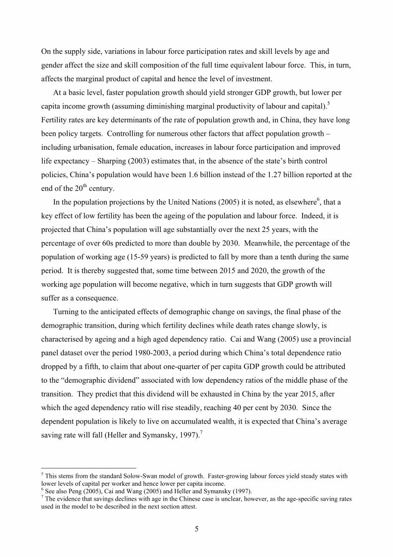
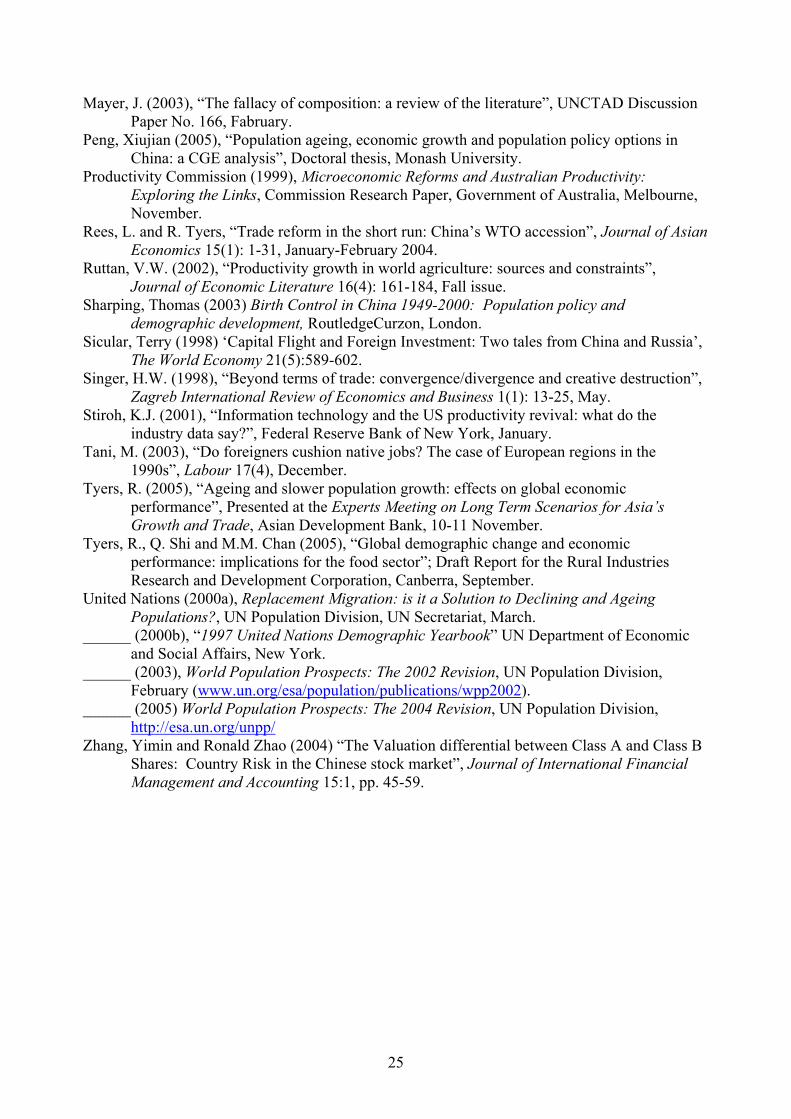
above the corresponding levels in the industrialised world. Indicative of this premium for the
case of China is the spread between its domestic bond yields and those of US Treasury bonds.
This is illustrated in Figure 1.
These “interest premia” have two components: a risk-free component, due to market
segmentation, and a risk premium. The risk-free component depends on capital controls and
other regulations that impair the free flow of financial capital across borders. De Jong and de
Roon (2005) analyse the impact that decreasing segmentation has had on thirty emerging stock
markets in the last two decades. They show that the average annual decrease in segmentation
(measured by the percentage of assets not available for foreign investors) has reduced the cost of
capital (measured by dividend yields) by about 11 basis points. Given that the Chinese stock
market was the most highly segmented of all the economies in the sample (averaging 86% 8 This is, indeed, the behaviour that emerges from our simulations, presented in Section 6. It contrasts with the work of Cheng (2003) who uses a numerical multi-period overlapping generations model for China through to 2030 and finds that there is no significant link between demography and per capita income growth (irrespective of financial capital mobility).
7
compared with 66% in South Korea, 18% in Malaysia and the lowest of 0.3% in Poland), these
results suggest substantial potential gains from reforms that successfully erode the degree of
segmentation.
The risk premium compensates investors for exchange rate risk, information asymmetries,
and perceived risks of expropriation. Fernald and Rogers (1998) develop an asset-pricing model
for China’s segmented stock market in which uncertainty is implicitly incorporated as an equity
risk premium in the required rate of return. They show that foreigners were paying only one
quarter of the domestic price for shares on China’s stock market in early 1998, and argue that this
is accounted for by an increase in the return they required, which may be caused by either an
increase in the risk-free real rate, an increase in the risk premium or both. Indeed at this time,
increased volatility and uncertainty led to higher required risk premia across the Asian region
(Fernald, Edison and Loungani, 1998).
Assessments of country risk – referring broadly to the likelihood that a sovereign state or
borrower from a particular country may be unable and/or unwilling to fulfil their obligations
towards one or more foreign lenders and/or investors – incorporate many economic, financial and
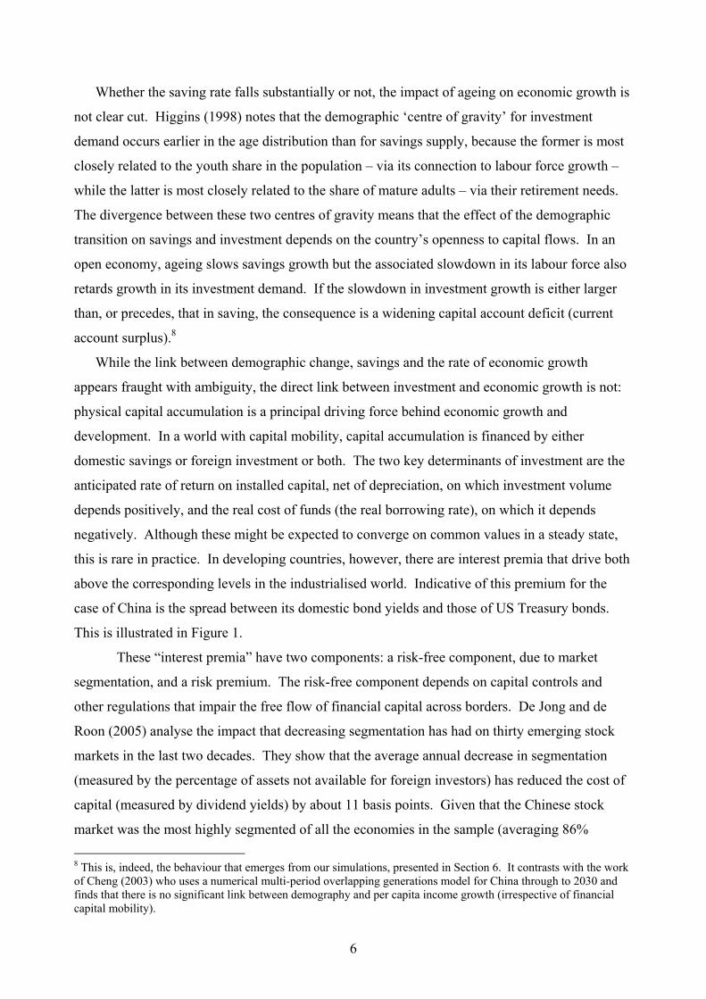
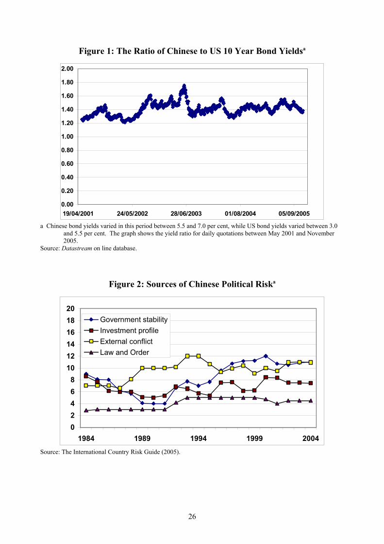
political factors (Hoti and McAleer, 2004). The International Country Risk Guide (2005) offers a
rating that comprises 22 variables in three categories – political, economic and financial – with
the political risk comprising 12 components and the economic and financial risk each comprising
five.9 Four of the key political components for China are plotted in Figure 2, illustrating a
volatile but generally upward trend in each, where higher scores equate to lower risk. While this
trend does not exist for all political variables (for example, democratic accountability worsened
throughout the 1990s), to the extent that lower risk ratings can be achieved we would expect this
trend to reduce China’s interest premium. Indeed, this is the conclusion from an analysis of asset
prices by Zhang and Zhao (2004). They focus on the divergence in Chinese A-share and B-share
prices over the period 1992-2000 and assess the determinants of stock price differentials. Their
key conclusion is that political risk is a significant determinant of the valuation differential
between Class A- and B-shares. Their findings also suggest that policy measures that reduce
either the degree of political (or country) risk or market segmentation will reduce investors’
required rates of return.
A complicating factor affecting China’s interest premia is that policies have tended to bias
the choice of the source of finance. Huang (2003) discusses how China’s economic policies
through to the turn of the 21st century were essentially biased in favour of foreign investment; the
9 See these described at http://www.prsgroup.com/icrg/icrg.html.
8
establishment of special economic zones being the key example. With central and local
governments providing such strong support and incentives for foreign investment, the perceived
risks of investing in China were lowered. Given that ongoing reforms and WTO concessions
should end this discrimination, it is quite possible that there will be an increase in the perceived
risks of investing in China, at least for foreigners. Yet Huang argues that the discrimination has
caused a “crowding out” of domestic by foreign direct investment, and that domestic investment
will rise to the occasion once the playing field is levelled. Overall, the net effect of financial
reforms on Chinese investment will depend upon their effects on incentives facing domestic
savers and foreign investors.
The bias in favour of foreign investment is seen by Sicular (1998) as fostering private
outflows of private financial capital. She attributes this to differences between residents’ and
non-residents’ returns to and risks of investing in China and notes that the limited opportunities
for locals to diversify their investment portfolios gives them the incentive to transfer savings
offshore if they think they can get away with it. If further reforms improve internal opportunities,
this could reduce the net outflows. On the other hand, the premature relaxation of capital controls
could have the reverse impact.
Clearly, much depends on continued market-oriented reforms, particularly in the financial
sector. Lardy (1998, 2003) argues that the reform of China’s financial system is one of the most
important decisions facing the Chinese leadership. Under the current system, declining
government revenues relative to GDP have meant that the government continues to force SOEs to
maintain excessive social obligations. In turn, state-owned banks have lent excessively to SOEs,
supported by extremely high household savings rates. Without urgently needed reforms, the
financial sector’s liabilities to households, which vastly exceed their assets, has the potential to
precipitate a financial crisis. This, more than anything, would lead to drastic increases in the risk
premium for investors in China, whether domestic or foreign.
3. Modelling the Economic Implications of Demographic Change The approach adopted follows Tyers (2005), in that it applies a complete demographic
sub-model that is integrated within a dynamic numerical model of the global economy.10 The
economic model is a development of GTAP-Dynamic, the standard version of which has single
10 See also Shi and Tyers (2004) and Tyers et al. (2005).
9
households in each region and therefore no demographic structure.11 The version used has
regional households with endogenous saving rates that are disaggregated by age group, gender
and skill level.
3.1 Demography:
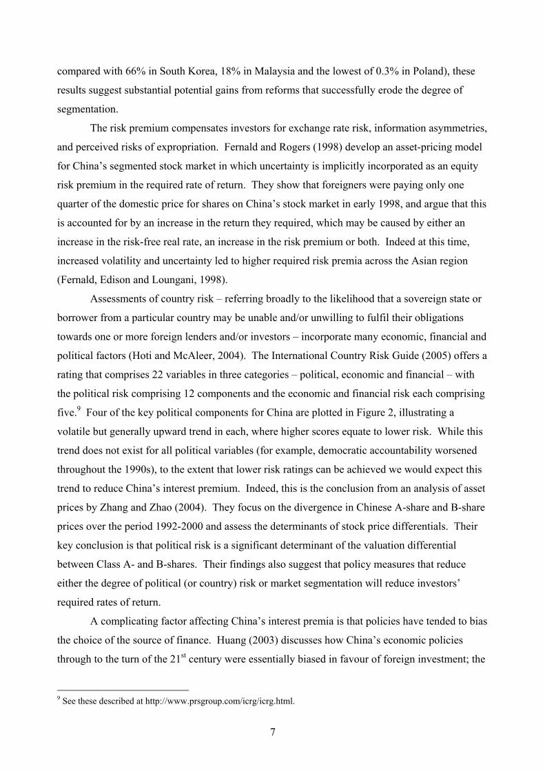
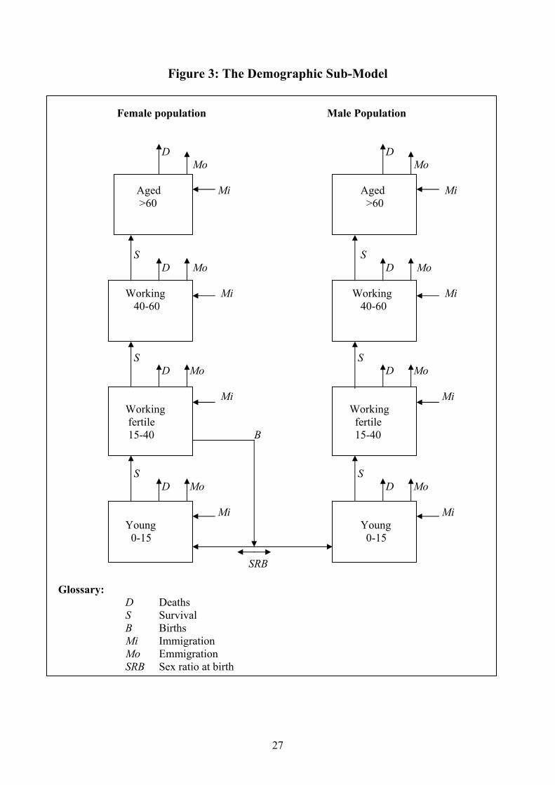
The demographic sub-model tracks populations in four age groups and two genders: a
total of 8 population groups in each of 14 regions.12 The four age groups are the dependent
young, adults of fertile and working age, older working adults and the mostly-retired over 60s.
The resulting age-gender structure is displayed in Figure 3. The population is further divided
between households that provide production labour and those providing professional labour.13
Each age-gender-skill group is a homogeneous sub-population with group-specific birth and
death rates and rates of both immigration and emigration.14 If the group spans T years, the
survival rate to the next age group is the fraction 1/T of its population, after group-specific deaths
have been removed and its population has been adjusted for net migration.
The final age group (60+) has duration equal to measured life expectancy at 60, which
varies across genders and regions. The key demographic parameters, then, are birth rates, sex
ratios at birth, age- and gender-specific death, immigration and emigration rates and life
expectancies at 60.15 A further key parameter is the rate at which each region’s education and
social development structure transforms production worker families into professional worker
families. Each year a particular proportion of the population in each production worker age-
gender group is transferred to professional status. These proportions depend on the regions’
levels of development, the associated capacities of their education systems and the relative sizes
of the production and professional labour groups.
In any year, for each age group, a, gender group g, skill group s, region of origin, r and
region of destination, d, the volume of migration flow is:
11 The GTAP-Dynamic model is a development of its comparative static progenitor, GTAP (Hertel et al. 1997). Its dynamics is described by Ianchovichina and McDougall (2000). Earlier applications of the standard model to the issues raised in this paper include those by Shi and Tyers (2004) and Duncan, Shi and Tyers (2005). 12 The demographic sub-model has been used in stand alone mode for the analysis of trends in dependency ratios. For a more complete documentation of the sub-model, see Chan and Tyers (2004). 13 The subdivision between production and professional labour accords with the ILO’s occupation-based classification and is consistent with the labour division adopted in the GTAP Database. See Liu et al. (1998). 14 Mothers in families providing production labour are assumed to produce children that will grow up to also provide production labour, while the children of mothers in professional families are correspondingly assumed to become professional workers. 15 Immigration and emigration are also age and gender specific. The model represents a full matrix of global migration flows for each age and gender group. Each of these flows is currently set at a constant proportion of the population of its destination group. See Tyers (2005) for further details.
10
(1) , , , , , , , , , , , , , , ,t t R ta g s r d d a g s r d a g s dM M N a g r dδ= ∀ ,
where tdδ is a destination-specific factor reflecting immigration policy in region d, R
agsrdM is the
migration rate between r and d expressed as a proportion of the group population in region d,
agsdN .
Given the migration matrix, agsrdM , the population in each age, gender and skill group and
region can be constructed. We begin with the population of males aged 0-14 from professional
families in region d (a=014, g=m, s=sk, r=d).
(2)
1 1014, , , 014, , , , 1539, , ,
1014, , , 014, , , 014, , , , 014, , , ,
1 1 1014, , , 014, , , 014, , , 014, , ,
1
1 ,15
tt t t td
m sk d m sk d sk d f sk dtd
t t t tm sk d m sk d m sk r d m sk d rr r
t t t td m unsk d m sk d m sk d m sk d
SN N B NS
D N M M
N N D N dρ
− −
−
− − −
= ++
− + −
+ − − ∀
∑ ∑
where tdS is the sex ratio at birth (the ratio of male to female births) in region d, t
dB is the birth
rate, 014, ,t
m dD the death rate and dρ is the rate at which region d’s educational institutions and
general development transform production into professional worker families. The final term is
survival to the corresponding 15-39 age group. In the corresponding equation for young males
from production worker families the penultimate term is negative.
For females in professional families in this age group the corresponding equation is:
(3)
1 1014, , , 014, , , , 1539, , ,
1014, , , 014, , , 014, , , , 014, , , ,
1 1 1014, , , 014, , , 014, , , 014, , ,
11
1 ,15
t t t tf sk d f sk d sk d f sk dt
d
t t t tf sk d f sk d f sk r d f sk d rr r
t t t td f unsk d f sk d f sk d f sk d
N N B NS
D N M M
N N D N dρ
− −
−
− − −
= ++
− + −
+ − − ∀
∑ ∑ .
For adults of gender g from professional families in the age group 15-39 the equation includes a
where the final term indicates that deaths from this group each year depend on its life expectancy
at 60, 60 , , ,t
g sk dL + . Again, the equation for aged production worker family members is the same
except that the skill transformation term is negative.
Sources and structure:
Key parameters in the model are the migration rates, , , , ,Ra g s r dM , birth rates, ,
ts rB , sex ratios
at birth, trS , death rates, , , ,
ta g s rD , life expectancies at 60, 60 , , ,
tg s rL + and the skill transformation
rates dρ . The migration rates are based on recent migration records and are held constant
through time.16 The skill transformation rates are based on changes during the decade prior to the
base year, 1997, in the composition of aggregate regional labour forces as between production
and professional workers. These are also held constant through time.17
Asymptotic trends in other parameters:
The birth rates, life expectancy at 60 and the age specific mortality rates all trend through
time asymptotically. For each age group, a, gender group, g, and region, r, a target rate is
identified.18 The parameters then approach these target rates with initial growth rates determined
by historical observation. In year t the birth rate of region r is:
16 The migration rates and the corresponding birth rates are listed in detail in Chan et al. (2005: Tables 2-5). 17 Note that, as regions become more advanced and populations in the production worker families become comparatively small, the skill transformation rate has a diminishing effect on the professional population. 18 In this discussion the skill index, s, is omitted because birth and death rates, and life expectancies at 60 do not vary by skill category in the version of the model used.
12
(8) ( )( )0 0 0 1t tr r Tgt rB B B B eβ= + − − ,
where the rate of approach, β, is calibrated from the historical growth rate:
(9) ( )( )0 01 0
00 0
1ˆ Tgt rr rr
r r
B B eB BBB B
β− −−= = , so that
(10) 0 0
0 0
ˆln 1 r r
Tgt r
B BB B
β
= − −
.
Labour force projections:
To evaluate the number of “full-time equivalent” workers we first construct labour force
participation rates, Pa,g,r by gender and age group for each region from ILO statistics on the
“economically active population”. We then investigate the proportion of workers that are part
time and the hours they work relative to each regional standard for full time work. The result is
the number of full time equivalents per worker, Fa,g,r. The labour force in region r is then:
(7) 60
, , ,1539
f unskt tr a g s r
a g m s sk
L L+
= = =
= ∑ ∑∑ where , , , , , , , , , , ,t t t ta g s r a r a g r a g r a g s rL P F Nµ= .
Here ,ta rµ is a shift parameter reflecting the influence of policy on participation rates. The time
superscript on , ,t
a g rP refers to the extrapolation of observed trends in these parameters.19
Asymptotic trends in labour force participation:
For each age group, a, gender group, g, and region, r, a target country is identified whose
participation rate is approached asymptotically. The rate of this approach is determined by the
initial rate of change. Thus, the participation rate takes the form:
(8) ( )( )0 0 0, , , , , , 1t t
a g r a g r Tgt a g rP P P P eβ= + − − ,
where the rate of approach, β, is calibrated from the initial participation growth rate:
(9) ( )( )0 01 0
, ,, , , ,0, , 0 0
, , , ,
1ˆ Tgt a g ra g r a g ra g r
a g r a g r
P P eP PP
P P
β− −−= = , so that
(10) 0 0, , , ,
0 0, ,
ˆln 1 a g r a g r
Tgt a g r
P PP P
β
= − −
.
Target rates are chosen from countries considered “advanced” in terms of trends in participation
rates. Where female participation rates are rising, therefore, Norway provides a commonly 19 Although part time hours may well also be trending through time, we hold F constant in the current version of the model.
13
chosen target because its female labour force participation rates are higher than for other
countries.20
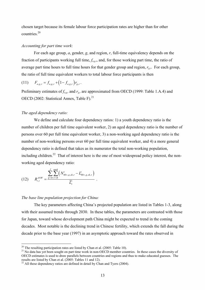
Accounting for part time work:
For each age group, a, gender, g, and region, r, full-time equivalency depends on the
fraction of participants working full time, fa,g,r, and, for those working part time, the ratio of
average part time hours to full time hours for that gender group and region, rg,r. For each group,
the ratio of full time equivalent workers to total labour force participants is then
(11) ( ), , , , , , ,1a g r a g r a g r g rF f f r= + − .
Preliminary estimates of fa,g,r and rg,r are approximated from OECD (1999: Table 1.A.4) and
OECD (2002: Statistical Annex, Table F).21
The aged dependency ratio:
We define and calculate four dependency ratios: 1) a youth dependency ratio is the
number of children per full time equivalent worker, 2) an aged dependency ratio is the number of
persons over 60 per full time equivalent worker, 3) a non-working aged dependency ratio is the
number of non-working persons over 60 per full time equivalent worker, and 4) a more general
dependency ratio is defined that takes as its numerator the total non-working population,
including children.22 That of interest here is the one of most widespread policy interest, the non-
working aged dependency ratio:
(12) ( )60 , , , 60 , , ,
,
f unskt t
g sk r g sk rg m s skANW
r t tr
N LR
L
+ += =
−=∑∑
.
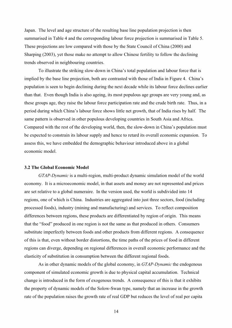
The base line population projection for China:
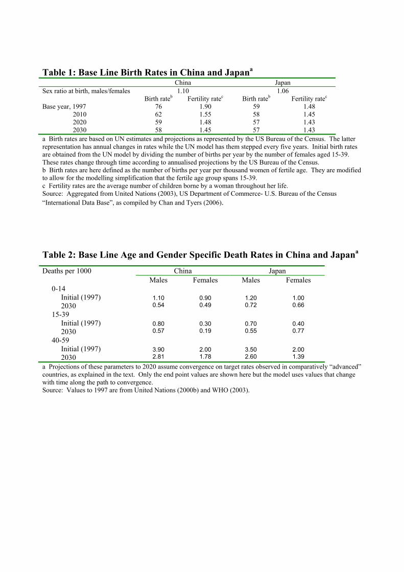
The key parameters affecting China’s projected population are listed in Tables 1-3, along
with their assumed trends through 2030. In these tables, the parameters are contrasted with those
for Japan, toward whose development path China might be expected to trend in the coming
decades. Most notable is the declining trend in Chinese fertility, which extends the fall during the
decade prior to the base year (1997) in an asymptotic approach toward the rates observed in
20 The resulting participation rates are listed by Chan et al. (2005: Table 10). 21 No data has yet been sought on part time work in non-OECD member countries. In these cases the diversity of OECD estimates is used to draw parallels between countries and regions and thus to make educated guesses. The results are listed by Chan et al. (2005: Tables 11 and 12). 22 All these dependency ratios are defined in detail by Chan and Tyers (2004).
14
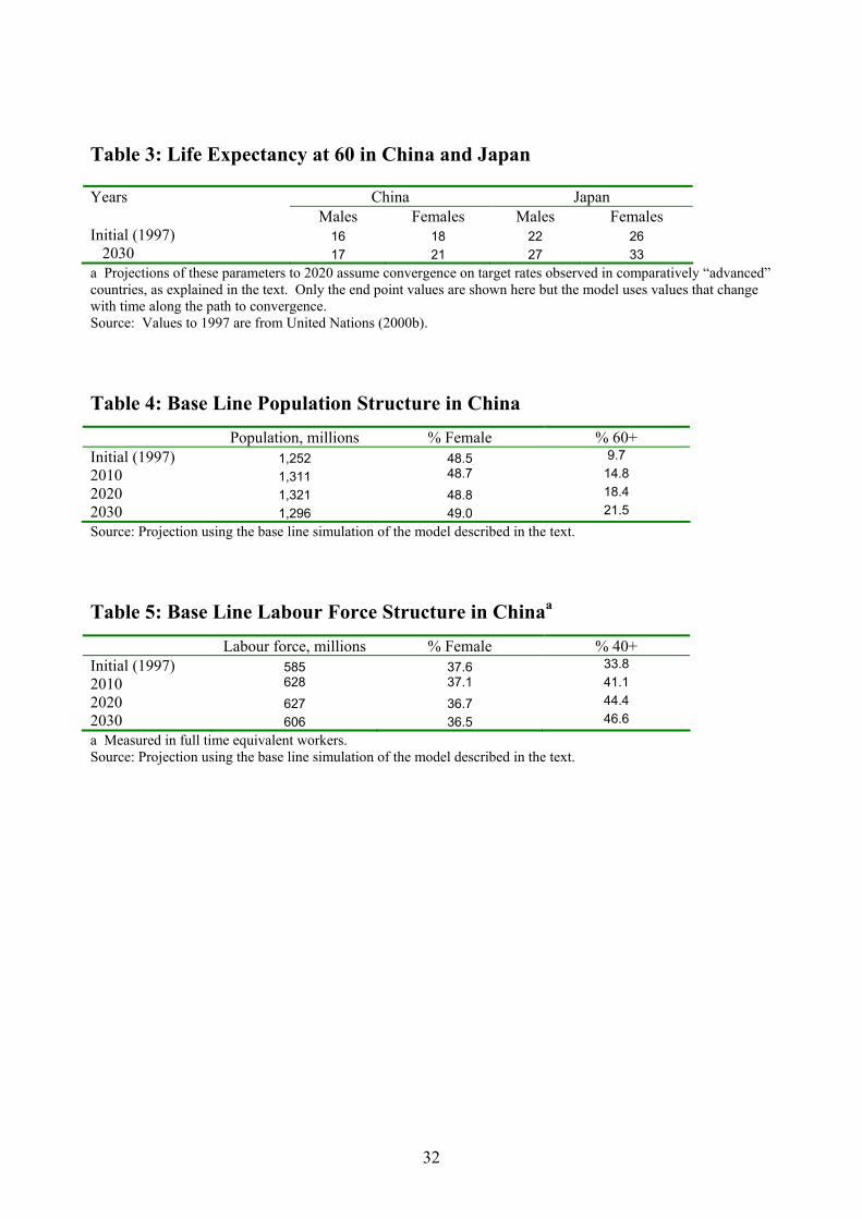
Japan. The level and age structure of the resulting base line population projection is then
summarised in Table 4 and the corresponding labour force projection is summarised in Table 5.
These projections are low compared with those by the State Council of China (2000) and
Sharping (2003), yet those make no attempt to allow Chinese fertility to follow the declining
trends observed in neighbouring countries.
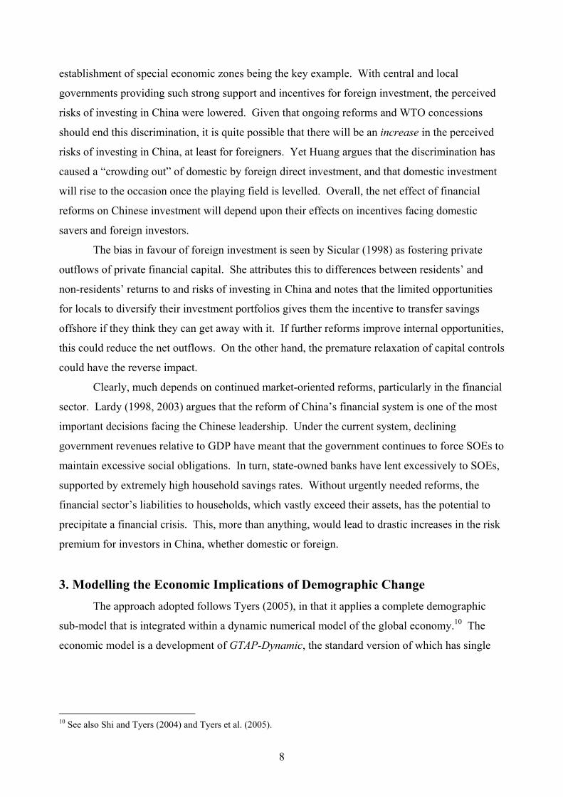
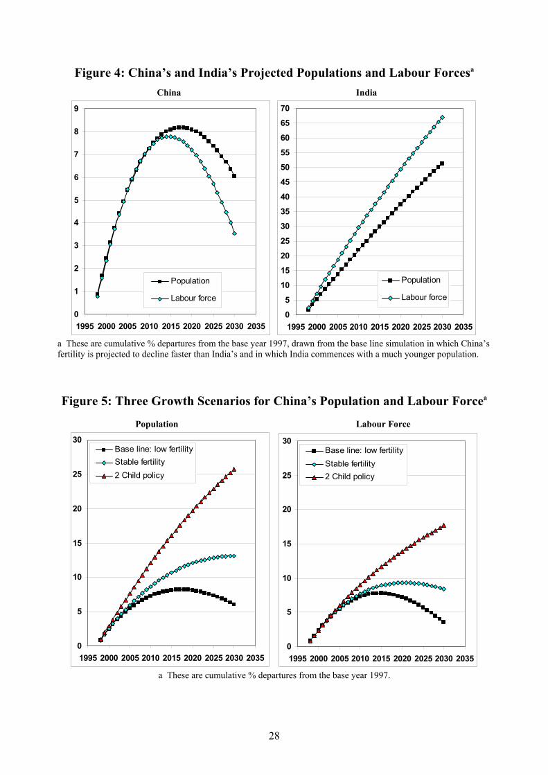
To illustrate the striking slow-down in China’s total population and labour force that is
implied by the base line projection, both are contrasted with those of India in Figure 4. China’s
population is seen to begin declining during the next decade while its labour force declines earlier
than that. Even though India is also ageing, its most populous age groups are very young and, as
these groups age, they raise the labour force participation rate and the crude birth rate. Thus, in a
period during which China’s labour force shows little net growth, that of India rises by half. The
same pattern is observed in other populous developing countries in South Asia and Africa.
Compared with the rest of the developing world, then, the slow-down in China’s population must
be expected to constrain its labour supply and hence to retard its overall economic expansion. To
assess this, we have embedded the demographic behaviour introduced above in a global
economic model.
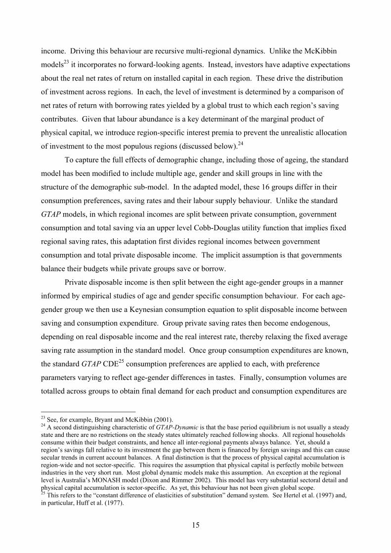
3.2 The Global Economic Model
GTAP-Dynamic is a multi-region, multi-product dynamic simulation model of the world
economy. It is a microeconomic model, in that assets and money are not represented and prices
are set relative to a global numeraire. In the version used, the world is subdivided into 14
regions, one of which is China. Industries are aggregated into just three sectors, food (including
processed foods), industry (mining and manufacturing) and services. To reflect composition
differences between regions, these products are differentiated by region of origin. This means
that the “food” produced in one region is not the same as that produced in others. Consumers
substitute imperfectly between foods and other products from different regions. A consequence
of this is that, even without border distortions, the time paths of the prices of food in different
regions can diverge, depending on regional differences in overall economic performance and the
elasticity of substitution in consumption between the different regional foods.
As in other dynamic models of the global economy, in GTAP-Dynamic the endogenous
component of simulated economic growth is due to physical capital accumulation. Technical
change is introduced in the form of exogenous trends. A consequence of this is that it exhibits
the property of dynamic models of the Solow-Swan type, namely that an increase in the growth
rate of the population raises the growth rate of real GDP but reduces the level of real per capita
15
income. Driving this behaviour are recursive multi-regional dynamics. Unlike the McKibbin
models23 it incorporates no forward-looking agents. Instead, investors have adaptive expectations
about the real net rates of return on installed capital in each region. These drive the distribution
of investment across regions. In each, the level of investment is determined by a comparison of
net rates of return with borrowing rates yielded by a global trust to which each region’s saving
contributes. Given that labour abundance is a key determinant of the marginal product of
physical capital, we introduce region-specific interest premia to prevent the unrealistic allocation
of investment to the most populous regions (discussed below).24
To capture the full effects of demographic change, including those of ageing, the standard
model has been modified to include multiple age, gender and skill groups in line with the
structure of the demographic sub-model. In the adapted model, these 16 groups differ in their
consumption preferences, saving rates and their labour supply behaviour. Unlike the standard
GTAP models, in which regional incomes are split between private consumption, government
consumption and total saving via an upper level Cobb-Douglas utility function that implies fixed
regional saving rates, this adaptation first divides regional incomes between government
consumption and total private disposable income. The implicit assumption is that governments
balance their budgets while private groups save or borrow.
Private disposable income is then split between the eight age-gender groups in a manner
informed by empirical studies of age and gender specific consumption behaviour. For each age-
gender group we then use a Keynesian consumption equation to split disposable income between
saving and consumption expenditure. Group private saving rates then become endogenous,
depending on real disposable income and the real interest rate, thereby relaxing the fixed average
saving rate assumption in the standard model. Once group consumption expenditures are known,
the standard GTAP CDE25 consumption preferences are applied to each, with preference
parameters varying to reflect age-gender differences in tastes. Finally, consumption volumes are
totalled across groups to obtain final demand for each product and consumption expenditures are
23 See, for example, Bryant and McKibbin (2001). 24 A second distinguishing characteristic of GTAP-Dynamic is that the base period equilibrium is not usually a steady state and there are no restrictions on the steady states ultimately reached following shocks. All regional households consume within their budget constraints, and hence all inter-regional payments always balance. Yet, should a region’s savings fall relative to its investment the gap between them is financed by foreign savings and this can cause secular trends in current account balances. A final distinction is that the process of physical capital accumulation is region-wide and not sector-specific. This requires the assumption that physical capital is perfectly mobile between industries in the very short run. Most global dynamic models make this assumption. An exception at the regional level is Australia’s MONASH model (Dixon and Rimmer 2002). This model has very substantial sectoral detail and physical capital accumulation is sector-specific. As yet, this behaviour has not been given global scope. 25 This refers to the “constant difference of elasticities of substitution” demand system. See Hertel et al. (1997) and, in particular, Huff et al. (1977).
16
subtracted from group disposable incomes to obtain group saving levels, which are then totalled
across groups to obtain regional saving.
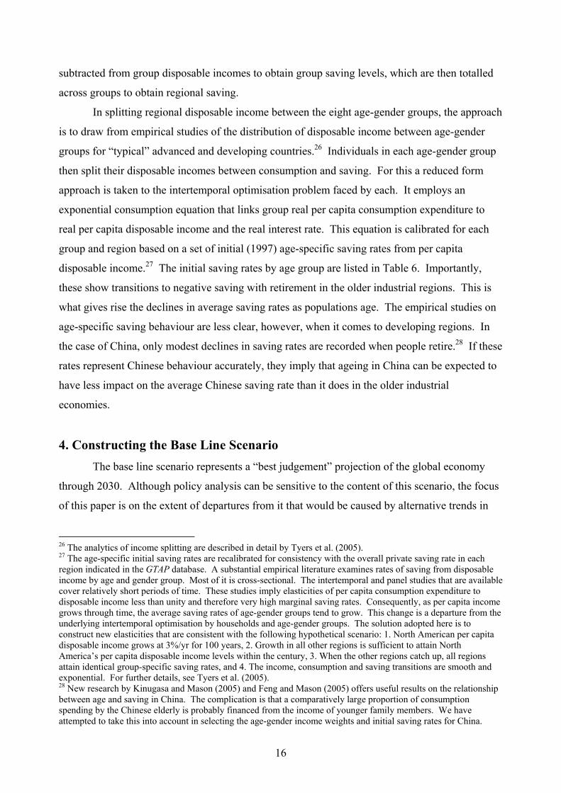
In splitting regional disposable income between the eight age-gender groups, the approach
is to draw from empirical studies of the distribution of disposable income between age-gender
groups for “typical” advanced and developing countries.26 Individuals in each age-gender group
then split their disposable incomes between consumption and saving. For this a reduced form
approach is taken to the intertemporal optimisation problem faced by each. It employs an
exponential consumption equation that links group real per capita consumption expenditure to
real per capita disposable income and the real interest rate. This equation is calibrated for each
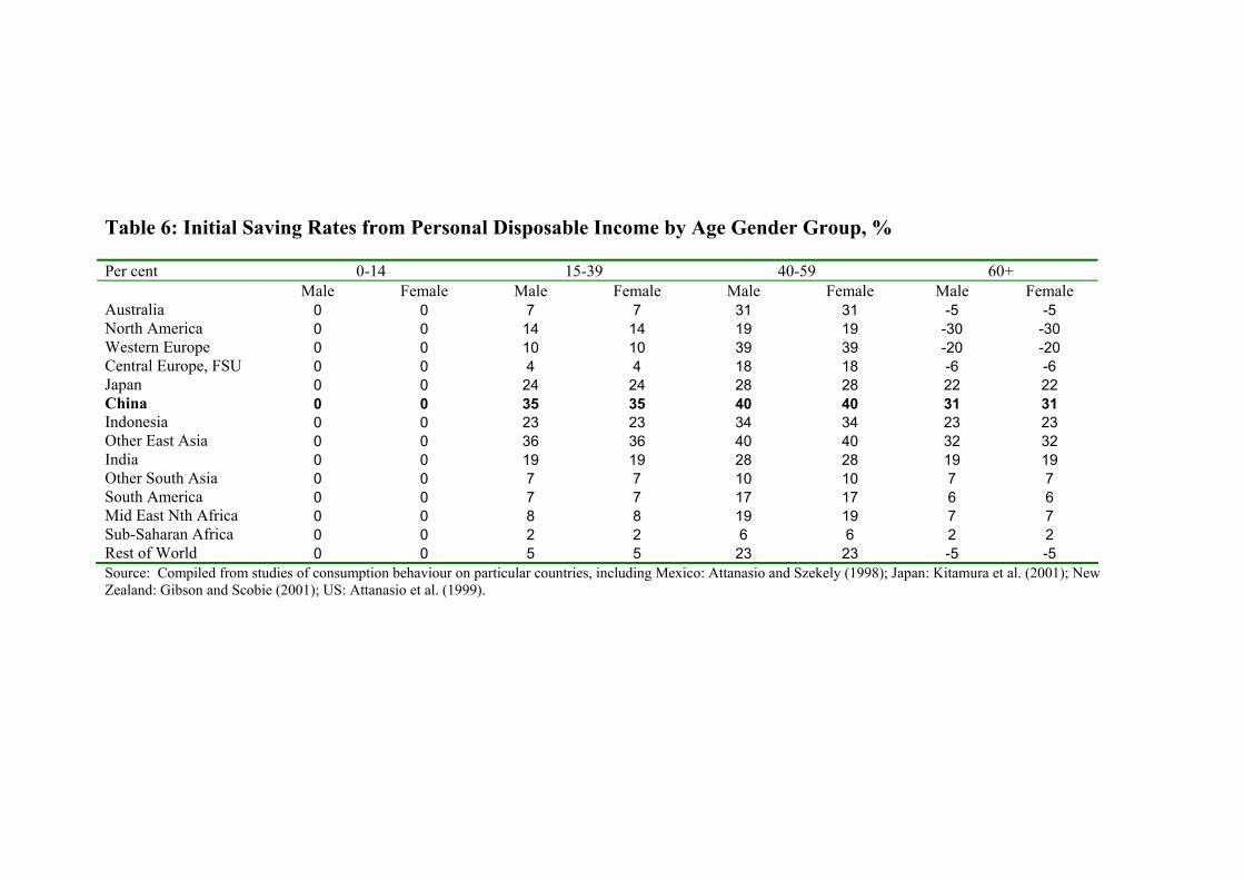
group and region based on a set of initial (1997) age-specific saving rates from per capita
disposable income.27 The initial saving rates by age group are listed in Table 6. Importantly,
these show transitions to negative saving with retirement in the older industrial regions. This is
what gives rise the declines in average saving rates as populations age. The empirical studies on
age-specific saving behaviour are less clear, however, when it comes to developing regions. In
the case of China, only modest declines in saving rates are recorded when people retire.28 If these
rates represent Chinese behaviour accurately, they imply that ageing in China can be expected to
have less impact on the average Chinese saving rate than it does in the older industrial
economies.
4. Constructing the Base Line Scenario The base line scenario represents a “best judgement” projection of the global economy
through 2030. Although policy analysis can be sensitive to the content of this scenario, the focus
of this paper is on the extent of departures from it that would be caused by alternative trends in
26 The analytics of income splitting are described in detail by Tyers et al. (2005). 27 The age-specific initial saving rates are recalibrated for consistency with the overall private saving rate in each region indicated in the GTAP database. A substantial empirical literature examines rates of saving from disposable income by age and gender group. Most of it is cross-sectional. The intertemporal and panel studies that are available cover relatively short periods of time. These studies imply elasticities of per capita consumption expenditure to disposable income less than unity and therefore very high marginal saving rates. Consequently, as per capita income grows through time, the average saving rates of age-gender groups tend to grow. This change is a departure from the underlying intertemporal optimisation by households and age-gender groups. The solution adopted here is to construct new elasticities that are consistent with the following hypothetical scenario: 1. North American per capita disposable income grows at 3%/yr for 100 years, 2. Growth in all other regions is sufficient to attain North America’s per capita disposable income levels within the century, 3. When the other regions catch up, all regions attain identical group-specific saving rates, and 4. The income, consumption and saving transitions are smooth and exponential. For further details, see Tyers et al. (2005). 28 New research by Kinugasa and Mason (2005) and Feng and Mason (2005) offers useful results on the relationship between age and saving in China. The complication is that a comparatively large proportion of consumption spending by the Chinese elderly is probably financed from the income of younger family members. We have attempted to take this into account in selecting the age-gender income weights and initial saving rates for China.
17
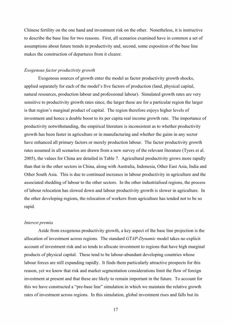
Chinese fertility on the one hand and investment risk on the other. Nonetheless, it is instructive
to describe the base line for two reasons. First, all scenarios examined have in common a set of
assumptions about future trends in productivity and, second, some exposition of the base line
makes the construction of departures from it clearer.
Exogenous factor productivity growth
Exogenous sources of growth enter the model as factor productivity growth shocks,
applied separately for each of the model’s five factors of production (land, physical capital,
natural resources, production labour and professional labour). Simulated growth rates are very
sensitive to productivity growth rates since, the larger these are for a particular region the larger
is that region’s marginal product of capital. The region therefore enjoys higher levels of
investment and hence a double boost to its per capita real income growth rate. The importance of
productivity notwithstanding, the empirical literature is inconsistent as to whether productivity
growth has been faster in agriculture or in manufacturing and whether the gains in any sector
have enhanced all primary factors or merely production labour. The factor productivity growth
rates assumed in all scenarios are drawn from a new survey of the relevant literature (Tyers et al.
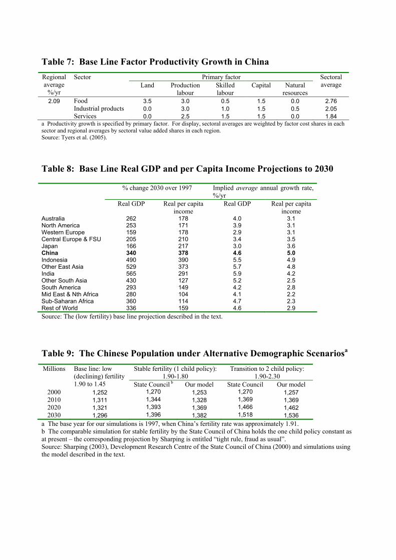
2005), the values for China are detailed in Table 7. Agricultural productivity grows more rapidly
than that in the other sectors in China, along with Australia, Indonesia, Other East Asia, India and
Other South Asia. This is due to continued increases in labour productivity in agriculture and the
associated shedding of labour to the other sectors. In the other industrialised regions, the process
of labour relocation has slowed down and labour productivity growth is slower in agriculture. In
the other developing regions, the relocation of workers from agriculture has tended not to be so
rapid.
Interest premia
Aside from exogenous productivity growth, a key aspect of the base line projection is the
allocation of investment across regions. The standard GTAP-Dynamic model takes no explicit
account of investment risk and so tends to allocate investment to regions that have high marginal
products of physical capital. These tend to be labour-abundant developing countries whose
labour forces are still expanding rapidly. It finds them particularly attractive prospects for this
reason, yet we know that risk and market segmentation considerations limit the flow of foreign
investment at present and that these are likely to remain important in the future. To account for
this we have constructed a “pre-base line” simulation in which we maintain the relative growth
rates of investment across regions. In this simulation, global investment rises and falls but its
18
allocation between regions is thus controlled. To do this the interest premium variable (GTAP
Dynamic variable SDRORT) is made endogenous. This creates wedges between the international
and regional interest rates. They show high interest premia for the populous developing regions
of Indonesia, India, South America and Sub-Saharan Africa. Premia tend to fall over time in
other regions, where labour forces are falling or growing more slowly. Most spectacular is a
secular fall in the Chinese premium. This is because the pre-base simulation maintains
investment growth in China despite the eventual decline in its labour force. This simulation is
therefore overly optimistic with respect to China and so we reject the declining premium in
constructing the final base line scenario. The time paths of all interest premia are set as
exogenous with China’s held constant through time. Regional investment is freed up in all
regions. The endogeneity of investment is an element of the model’s closure that is maintained in
all subsequent simulations.
The base line projection
Overall base line economic performance is suggested by Table 8, which details the
average GDP and real per capita income growth performance of each region from 1997 to 2030.
In part because of its comparatively young population and hence its continuing rapid labour force
growth, India attracts substantial new investment and is projected to take over from China as the
world’s most rapidly expanding region. Rapid population growth detracts from India’s real per
capita income performance, however. By this criterion, China is the strongest performing region
through the three decades. Indonesia and “other East Asia” are also strong performers, while the
older industrial economies continue to grow more slowly. The African regions enjoy good GDP
growth performance but their high population growth rates limit their performance in per capita
terms.
5. Alternative Demographic Scenarios for China Following Sharping (2003) and the State Council of China (2000), two higher-fertility
scenarios are constructed. These differ only in their fertility rates. Death rates and migration
behaviour are assumed to remain as in the base line projection. The first higher-fertility scenario
offers a comparatively stable Chinese birth rate, with the fertility rate trending from 1.90 to 1.80
over the three decades to 2030. It is similar to the State Council “one child policy”, and to
Sharping’s “tight rule, fraud as usual” scenario. The second trends toward two children per
couple throughout China, with a fertility rate of 2.3 achieved by 2030. It is similar to the State
19
Council’s “two child policy” and to Sharping’s “delayed two child policy …”. The implications
for China’s total population under these scenarios are indicated in Table 9.
The correspondence between these simulations and State Council projections is close. A
transition to a two-child policy would raise the 2030 population by 11 per cent relative to the
stable fertility case. Our low-fertility base line, on the other hand, achieves a 2030 population
seven per cent below the stable fertility case. These implications are displayed graphically in
Figure 5. Critically, the associated labour force changes are smaller in magnitude and transitions
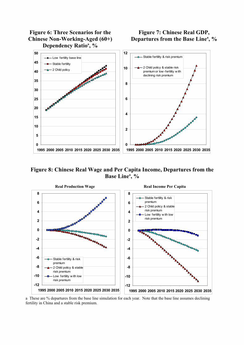
occur earlier than those in the populations. The Chinese population ages in all three scenarios,
but more slowly the higher the fertility rate. This can be seen from the non-working-aged
dependency ratio in Figure 6. It rises substantially by 2030 in all three cases. After 2015,
however, there are discernable differences, with the two-child policy yielding a 2030 ratio that is
lower by four percentage points than the low-fertility base line.
Economic Implications:
The three main avenues through which higher fertility affects economic performance are
via the labour force, which it expands, the savings share of income, which tends to rise with the
share of the population of working age, and the product composition of consumption, which more
strongly reflects the preferences of the young when population growth accelerates. The
comparisons made by Tyers et al. (2005) suggest a general ranking that has the labour force
avenue most commonly the strongest with the saving rate avenue next and with the influence of
age-specific consumption preferences comparatively small. This is indeed borne out. The labour
force effect can first be seen through it impact on the non-working-aged dependency ratio. This
ratio expands under all scenarios in China, as shown in Figure 6, but it grows least in the two-
child policy case.29
Turning to the other avenues, age-specific consumption preferences can be expected to
have little influence in the results presented here since product markets are aggregated into three
broad sectors and the capturing of generational differences in preferences requires fine product
detail. As to the saving rate, for reasons discussed previously the effects of Chinese fertility
changes on average saving rates can be expected to be smaller than they are in the older
industrialised regions. Beyond the dependency ratio, the dominant economic theme might
therefore be changes in China’s labour force that alter the productivity of its capital and therefore
29 This result could have a number of economic implications that are not captured in our model, including that higher fertility would necessitate lower rates of distorting taxes to finance aged pensions and public health systems. Our scenarios maintain constant tax rates and fiscal deficits.
20
the return on Chinese investment. Greater population growth thereby attracts an increased share
of the world’s savings into Chinese investment and so China’s capital stock grows more rapidly.
China’s GDP might therefore be expected to be boosted substantially by increased fertility,
through its direct and indirect influence over the supply of the two main factors of production,
labour and capital. In per capita terms, however, the Solow-Swan predisposition toward slower
real wage growth, combined with the need to reward foreign capital owners, suggests that the
average Chinese will not derive economic benefit from increased fertility.
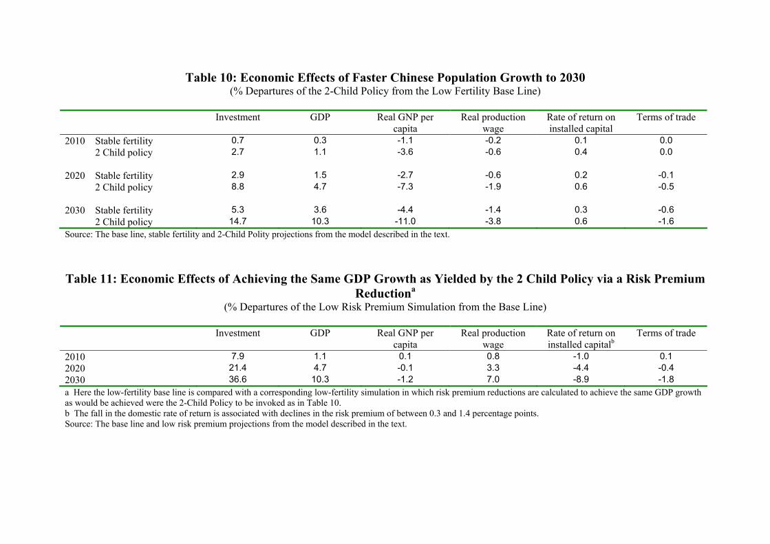
These expectations are indeed borne out in our simulations, as indicated in Table 10.
Higher fertility, relative to the base line, does raise the rate of return on installed capital in China
and hence the level of investment. In turn, China’s GDP is higher, as is also shown in Figure 7.
Yet the higher fertility slows real wage growth, due to the increased relative abundance of labour
and, in combination with the repatriation of an increased proportion of the income accruing to
capital, this causes real per capita income also to grow more slowly. A further negative
complication is the large-country effect – as China’s trade with the rest of the world expands it
turns its terms of trade against itself. This effect is small overall but of growing significance late
in the period.30 The corresponding dynamics of the real production wage and real per capital
income are illustrated in Figure 8.
6. Faster GDP Growth by Reducing China’s Interest Premium Here we ask how different the economic changes would be were fertility to remain low, as
in the base line, and were the GDP growth achieved under the two-child policy to be gained
instead by a decline in China’s interest premium. To find this out we change the closure of the
model by setting China’s GDP growth path as exogenous and making China’s interest premium
endogenous. Otherwise the simulation is identical with the base line. With this change in
closure, the model tells us by how much China’s interest premium would need to fall. This
magnitude, and the other economic implications of achieving higher growth through a reduced
premium, are summarised in Table 11.
The new simulation of the global economy approaches a steady state by 2030, in that the
bond yield that equates global saving with global investment as adjusted by China’s remaining
interest premium converges with the net rate of return on installed capital in China. To achieve
30 Empirical evidence for such terms of trade effects from growth is variable. In many cases, developing country expansions have not caused adverse shifts in their terms of trade because their trade has embraced new products and quality ladders in ways not captured by our model. See the literature on the developing country exports fallacy of composition argument, that includes Lewis (1952), Grilli and Yang (1988), Martin (1993), Singer (1998) and Mayer (2003).
21
GDP growth equivalent to the two-child policy case these rates need to be lower by almost a
tenth. Considering that the yield ratio of Chinese to US Treasury 10-year bonds has been about
1.4, as shown in Figure 1, there is, ultimately, scope for a decline of 28 per cent, this change
appears readily achievable with continued Chinese development and financial reform over three
decades.31
This acceleration in growth occurs because the reduced premium lowers the cost of funds
in China. Recall that investment depends positively on the net rate of return on installed capital
and negatively on the bond rate. Cheaper funds therefore spur investment, which, by 2030, is
larger than the base line by more than a third. This creates the principal distinction between this
simulation and that for the two-child policy. The latter spurs China’s GDP growth by raising its
labour endowment, while this simulation does so by accelerating the growth in its capital stock.
The two-child policy causes real wages to grow more slowly and for the increased labour
abundance to raise capital returns. On the other hand, the financial reform simulation sees real
wages accelerating and capital returns falling. Interestingly, although this alters the composition
of China’s imports and exports, the two simulations yield similar small deteriorations in China’s
terms of trade.
A key bottom line is the effect of each policy scenario on real income per capita. As
illustrated in Figure 8, the two-child policy slows real per capita income growth for reasons
discussed previously. The financial reform simulation achieves the same GDP growth without
this loss in per capita welfare relative to the low-fertility base line. It does so despite the slower
growth in capital returns that stem from the faster capital accumulation.32
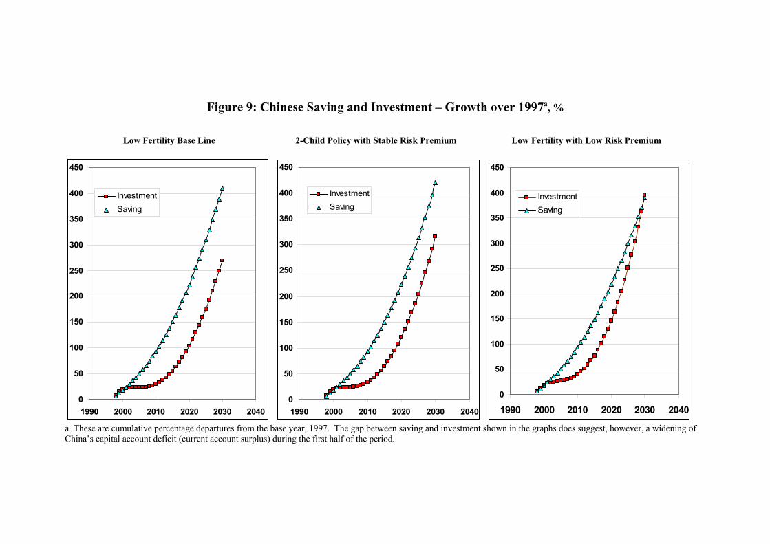
Superficially, one might expect that the accelerated build-up of the capital stock might be
at least partially financed from abroad and, therefore, that an increasing share of China’s capital
income would accrue to foreigners. A closer look shows that this is not the case. In all the
scenarios considered here China is projected to maintain a capital account deficit, and hence a
current account surplus, through 2030. This capital account deficit enlarges in the first half of the
period, as suggested by the plots shown in Figure 9, and either stabilises or contracts thereafter.
Small changes in saving rates, notwithstanding demographic change, and a high rate of income
growth ensure that total Chinese saving continues to grow to an extent that varies little across the
scenarios. As indicated earlier, it is the demographic effects on the labour force that make the
most difference. These change capital returns so that the two-child policy draws in more 31 See footnote 3. 32 A caveat applies here, however. To the extent that the initial interest premium is due to risk rather than to market segmentation, the cost of this risk is not accounted for in our deterministic model. Were that initial burden of risk to be properly measured, average net capital returns might not fall as much as predicted by the model.
22
investment and the capital account deficit tends to close. Reducing the interest premium,
however, has the most dramatic impact on China’s external accounts. This financial reform
scenario, with its accelerated capital accumulation, is seen to roughly close the capital account
deficit by the end of the period.
7. Conclusion China's economic growth has, hitherto, depended on its relative abundance of production
labour and its increasingly secure investment environment. Within the next decade, however,
China's labour force will begin to contract. This will set its economy apart from other developing
Asian countries where relative labour abundance will increase, as will relative capital returns.
This expectation is confirmed in this paper using a new global demographic model that is
integrated with an adaptation of the GTAP-Dynamic global economic model in which regional
households are disaggregated by age and gender. Unless there is a substantial change in
population policy, the retention of China's large share of global FDI will require reduced interest
premia and hence the successful continuation of financial reforms. A transition to a two child
policy in China is shown to boost its GDP growth, enlarging the projected 2030 Chinese
economy by about a tenth. Yet this would slow the growth rate of real per capita income,
reducing the level projected for 2030 by a tenth.
The same GDP growth performance might be achieved with continued low fertility, if
China’s interest premium can be reduced gradually through 2030, sufficiently to contract the
average domestic borrowing rate in 2030 by nine per cent. Considering that the yield ratio of
Chinese to US Treasury 10-year bonds has been about 1.4, there is, ultimately, scope for a decline
of 28 per cent, whihc appears achievable with continued Chinese development and financial
reform over three decades. This confirms that continued financial reform should take priority
over increased fertility.
Yet, even if financial sector reforms proceed smoothly, there is no guarantee that this will
immediately either reduce the risks of investing, or increase the volume of investment. In the
long-run, reforms should result in the allocation of funds to higher productivity sectors –
particularly the private sector – yielding efficiency gains and raising the returns to investment.
But in short-run, the shift away from a state-controlled banking system, in which the government
has implicitly guaranteed bank loans to loss-making SOEs and also provided incentives to attract
foreign investors, may actually increase the risks associated with investing in China. Perversely,
this could worsen the investment environment, in the short-run at least. For domestic investors,
23
the opening of the financial sector to foreign institutions will provide alternative investment
opportunities, which may lead them to require greater returns from state-owned assets or to find
new means of channelling their capital outside the country. Ultimately, successful financial
reforms will be those that attract domestic savings to China’s financial markets, while maitaining
a high level of foreign investment.
References Bloom, D.E. and J.G. Williamson (1997), “Demographic transitions, human resource
development and economic miracles in emerging Asia”, in J. Sachs and D. Bloom (eds.), Emerging Asia, Manila: Asian Development Bank.
Bryant, R.C. and W.J. McKibbin (1998), “Issues in modelling the global dimensions of demographic change”, http://www.sensiblepolicy.com/wmhp/home1.htm .
________ (2001), “Incorporating demographic change in multi-country demographic models: some preliminary results”, http://www.sensiblepolicy.com/wmhp/home1.htm .
Cai Fang and Dewen Wang (2005) ‘Demographic Transition: implications for growth’ in Garnaut and Song, eds, The China Boom and its Discontents, Asia-Pacific Press, Canberra.
Cheng, Kevin (2003) ‘Economic Implications of China’s Demographics in the 21st century’, IMF Working Paper WP/03/29
Chan, M.M., J. Pant and R. Tyers (2005), “Global demographic change and labour force growth: projections to 2020”, Centre for Economic Policy Research Discussion Paper, Research School of Social Sciences (RSSS), Australian National University, December.
De Jong, Frank and Frans A de Roon (2005), “Time-varying market integration and expected returns in emerging markets”, Journal of Financial Economics 78: 583-613
Development Research Centre of the State Council of China (2000), China Development Studies: the Selected Research Report of the Development Research Centre of the State Council, China Development Press.
Dixon, P.B. and M. Rimmer (2002), Dynamic General Equilibrium Modelling for Forecasting and Economic Policy, No. 256 in the Contributions for Economic Analysis series, published by Elsevier North Holland.
Duncan, R. and C. Wilson (2004), Global Population Projections: is the UN getting it wrong? Rural Industries Research and Development Corporation report No 04/041, RIRDC, Canberra.
Feng, W. and A. Mason (2005), “Demographic Dividend and Prospects for Economic Development in China”, UN Expert Group Meeting on Social and Economic Implications of Changing Population Age Structures, Mexico City, August 21-September 2.
Fernald, John G. and Oliver D. Babson (1999), “Why has China survived the Asian crisis so well? What risks remain?”, Board of Governors of the Federal Reserve System, International Finance Discussion Papers, No. 633, February.
Fernald, John, Hali Edison and Prakash Loungani (1998) ‘Was China the First Domino? Assessing Links between China and the rest of Emerging Asia’, Finance Division of the Federal Reserve Board, Washington DC.
Fernald, John and John Rogers (1998) “Puzzles in the Chinese Stock Market” International Finance Discussion Papers No. 619, August, Board of Governors of the Federal Reserve System.
24
Grilli, E. and M.C.Yang (1988), "Primary Commodity Prices, Manufactured Goods Prices and the Terms of Trade of Developing Countries: What the Long Run Shows", World Bank Economic Review, 2(1), January.
Gunter, Frank (2004) “Capital Flight from China: 1984-2001”, China Economic Review, 15: 63-85.
Harrigan, J. (1995), “The volume of trade in differentiated products: theory and evidence”, Review of Economics and Statistics 77(2): 283-293, May.
Hatton, T. and M. Tani (2003), “Immigration and Inter-Regional Mobility in the UK, 1982-2000”, Discussion Paper 4061, Centre for Economic Policy Research, London, September.
Heller, Peter and Steve Symansky (1997) “Implications for Savings of Aging in the Asian “Tigers””, IMF Working Paper, WP/97/136, October.
Hertel, T.W. (ed.), Global Trade Analysis Using the GTAP Model, New York: Cambridge University Press, 1997 (http://www.agecon.purdue.edu/gtap).
Higgins, Matthew (1998) “Demography, National Savings and International Capital Flows”, International Economic Review, Vol. 39, No. 2: 343-369, May.
Hoti, Suheljla and Michael McAleer (2004) “An empirical assessment of country risk ratings and associated models”, Journal of Economic Surveys, Vol. 18, No.4: 539-588.
Huang, Yasheng (2003) Selling China, Cambridge University Press, Cambridge, UK. Ianchovichina, E., R. Darwin and R. Shoemaker (2001), “Resource use and technological
progress in agriculture: a dynamic general equilibrium analysis”, Ecological Economics 38: 275-291.
Ianchovichina, E. and R. McDougall (2000), “Theoretical structure of Dynamic GTAP”, GTAP Technical Paper No.17, Purdue University, December (http://www.agecon.purdue.edu/gtap/GTAP-Dyn).
IMF (2004), World Economic Outlook, International Monetary Fund, Washington, DC, September.
Kinugasa, T. and A. Mason (2005), “The effects of adult longevity on saving”, mimeo, University of Hawaii at Manoa.
Khoo, S.E. and P. McDonald (2002), "Adjusting for change of status in international migration: demographic implications", International Migration, 40 (4): 103-124.
________ (eds.) (2003), The Transformation of Australia's Population, 1970-2030, Sydney: University of New South Wales Press, 302 pp.
Lardy, Nicolas (1998) China’s Unfinished Economic Revolution, Brookings Institution Press, Washington D.C.
________ (2002) Integrating China into the Global Economy, Brookings Institution Press, Washington D.C.
Lee, R. D. (2003), “The demographic transition: three centuries of fundamental change”, Journal of Economic Perspectives 17(4): 167-190.
Lewis, W.A. (1952) “World Production, Prices and Trade, 1870- 1960”, Manchester School of Economic and Social Sciences, 20(2):105-38, May.
Lipsey, R.E. (1994) “Quality Change and Other Influences on Measures of Export Prices of Manufactured Goods” World Bank Policy Research Working Paper 1348, Washington DC.
Liu, J. N. Van Leeuwen, T.T. Vo, R. Tyers, and T.W. Hertel (1998), “Disaggregating Labor Payments by Skill Level in GTAP”, Technical Paper No.11, Center for Global Trade Analysis, Department of Agricultural Economics, Purdue University, West Lafayette, September.
Martin, W. (1993), “The fallacy of composition and developing country exports of manufactures”, The World Economy 23: 979-1003.
25
Mayer, J. (2003), “The fallacy of composition: a review of the literature”, UNCTAD Discussion Paper No. 166, Fabruary.
Peng, Xiujian (2005), “Population ageing, economic growth and population policy options in China: a CGE analysis”, Doctoral thesis, Monash University.
Productivity Commission (1999), Microeconomic Reforms and Australian Productivity: Exploring the Links, Commission Research Paper, Government of Australia, Melbourne, November.
Rees, L. and R. Tyers, “Trade reform in the short run: China’s WTO accession”, Journal of Asian Economics 15(1): 1-31, January-February 2004.
Ruttan, V.W. (2002), “Productivity growth in world agriculture: sources and constraints”, Journal of Economic Literature 16(4): 161-184, Fall issue.
Sharping, Thomas (2003) Birth Control in China 1949-2000: Population policy and demographic development, RoutledgeCurzon, London.
Sicular, Terry (1998) ‘Capital Flight and Foreign Investment: Two tales from China and Russia’, The World Economy 21(5):589-602.
Singer, H.W. (1998), “Beyond terms of trade: convergence/divergence and creative destruction”, Zagreb International Review of Economics and Business 1(1): 13-25, May.
Stiroh, K.J. (2001), “Information technology and the US productivity revival: what do the industry data say?”, Federal Reserve Bank of New York, January.
Tani, M. (2003), “Do foreigners cushion native jobs? The case of European regions in the 1990s”, Labour 17(4), December.
Tyers, R. (2005), “Ageing and slower population growth: effects on global economic performance”, Presented at the Experts Meeting on Long Term Scenarios for Asia’s Growth and Trade, Asian Development Bank, 10-11 November.
Tyers, R., Q. Shi and M.M. Chan (2005), “Global demographic change and economic performance: implications for the food sector”; Draft Report for the Rural Industries Research and Development Corporation, Canberra, September.
United Nations (2000a), Replacement Migration: is it a Solution to Declining and Ageing Populations?, UN Population Division, UN Secretariat, March.
______ (2000b), “1997 United Nations Demographic Yearbook” UN Department of Economic and Social Affairs, New York.
______ (2003), World Population Prospects: The 2002 Revision, UN Population Division, February (www.un.org/esa/population/publications/wpp2002).
______ (2005) World Population Prospects: The 2004 Revision, UN Population Division, http://esa.un.org/unpp/
Zhang, Yimin and Ronald Zhao (2004) “The Valuation differential between Class A and Class B Shares: Country Risk in the Chinese stock market”, Journal of International Financial Management and Accounting 15:1, pp. 45-59.
26
Figure 1: The Ratio of Chinese to US 10 Year Bond Yieldsa
a Chinese bond yields varied in this period between 5.5 and 7.0 per cent, while US bond yields varied between 3.0 and 5.5 per cent. The graph shows the yield ratio for daily quotations between May 2001 and November 2005.
Source: Datastream on line database.
Figure 2: Sources of Chinese Political Riska
02468
101214161820
1984 1989 1994 1999 2004
Government stabilityInvestment profileExternal conflictLaw and Order
Source: The International Country Risk Guide (2005).
27
Figure 3: The Demographic Sub-Model
Female population Male Population D D Mo Mo Aged Mi Aged Mi >60 >60 S S D Mo D Mo Working Mi Working Mi 40-60 40-60 S S D Mo D Mo Mi Mi Working Working fertile fertile 15-40 B 15-40 S S D Mo D Mo Mi Mi Young Young 0-15 0-15 SRB Glossary: D Deaths S Survival B Births Mi Immigration Mo Emmigration SRB Sex ratio at birth
28
Figure 4: China’s and India’s Projected Populations and Labour Forcesa
China India
0
1
2
3
4
5
6
7
8
9
1995 2000 2005 2010 2015 2020 2025 2030 2035
Population
Labour force
0
5
10
15
20
25
30
35
40
45
50
55
60
65
70
1995 2000 2005 2010 2015 2020 2025 2030 2035
Population
Labour force
a These are cumulative % departures from the base year 1997, drawn from the base line simulation in which China’s fertility is projected to decline faster than India’s and in which India commences with a much younger population. Figure 5: Three Growth Scenarios for China’s Population and Labour Forcea
Population Labour Force
0
5
10
15
20
25
30
1995 2000 2005 2010 2015 2020 2025 2030 2035
Base line: low fertilityStable fertility2 Child policy
0
5
10
15
20
25
30
1995 2000 2005 2010 2015 2020 2025 2030 2035
Base line: low fertilityStable fertility2 Child policy
a These are cumulative % departures from the base year 1997.
Figure 6: Three Scenarios for the Chinese Non-Working-Aged (60+)
Dependency Ratioa, %
Figure 7: Chinese Real GDP, Departures from the Base Linea, %
0
5
10
15
20
25
30
35
40
45
50
1995 2000 2005 2010 2015 2020 2025 2030 2035
Low fertility base line
Stable fertility
2 Child policy
0
2
4
6
8
10
12
1995 2000 2005 2010 2015 2020 2025 2030 2035
Stable fertility & risk premium
2 Child policy & stable riskpremium or low -fertility w ithdeclining risk premium
Figure 8: Chinese Real Wage and Per Capita Income, Departures from the Base Linea, %
a These are % departures from the base line simulation for each year. Note that the base line assumes declining fertility in China and a stable risk premium.
Figure 9: Chinese Saving and Investment – Growth over 1997a, % Low Fertility Base Line 2-Child Policy with Stable Risk Premium Low Fertility with Low Risk Premium
0
50
100
150
200
250
300
350
400
450
1990 2000 2010 2020 2030 2040
InvestmentSaving
0
50
100
150
200
250
300
350
400
450
1990 2000 2010 2020 2030 2040
InvestmentSaving
0
50
100
150
200
250
300
350
400
450
1990 2000 2010 2020 2030 2040
InvestmentSaving
a These are cumulative percentage departures from the base year, 1997. The gap between saving and investment shown in the graphs does suggest, however, a widening of China’s capital account deficit (current account surplus) during the first half of the period.
Table 1: Base Line Birth Rates in China and Japana
China Japan Sex ratio at birth, males/females 1.10 1.06 Birth rateb Fertility ratec Birth rateb Fertility ratec
Base year, 1997 76 1.90 59 1.48 2010 62 1.55 58 1.45 2020 59 1.48 57 1.43 2030 58 1.45 57 1.43 a Birth rates are based on UN estimates and projections as represented by the US Bureau of the Census. The latter representation has annual changes in rates while the UN model has them stepped every five years. Initial birth rates are obtained from the UN model by dividing the number of births per year by the number of females aged 15-39. These rates change through time according to annualised projections by the US Bureau of the Census. b Birth rates are here defined as the number of births per year per thousand women of fertile age. They are modified to allow for the modelling simplification that the fertile age group spans 15-39. c Fertility rates are the average number of children borne by a woman throughout her life. Source: Aggregated from United Nations (2003), US Department of Commerce- U.S. Bureau of the Census “International Data Base”, as compiled by Chan and Tyers (2006).
Table 2: Base Line Age and Gender Specific Death Rates in China and Japana
China Japan Deaths per 1000 Males Females Males Females
0-14 Initial (1997) 1.10 0.90 1.20 1.00 2030 0.54 0.49 0.72 0.66 15-39 Initial (1997) 0.80 0.30 0.70 0.40 2030 0.57 0.19 0.55 0.77 40-59 Initial (1997) 3.90 2.00 3.50 2.00 2030 2.81 1.78 2.60 1.39 a Projections of these parameters to 2020 assume convergence on target rates observed in comparatively “advanced” countries, as explained in the text. Only the end point values are shown here but the model uses values that change with time along the path to convergence. Source: Values to 1997 are from United Nations (2000b) and WHO (2003).
32
Table 3: Life Expectancy at 60 in China and Japan
China Japan Years Males Females Males Females
Initial (1997) 16 18 22 26 2030 17 21 27 33 a Projections of these parameters to 2020 assume convergence on target rates observed in comparatively “advanced” countries, as explained in the text. Only the end point values are shown here but the model uses values that change with time along the path to convergence. Source: Values to 1997 are from United Nations (2000b).
Table 4: Base Line Population Structure in China Population, millions % Female % 60+
a Productivity growth is specified by primary factor. For display, sectoral averages are weighted by factor cost shares in each sector and regional averages by sectoral value added shares in each region. Source: Tyers et al. (2005). Table 8: Base Line Real GDP and per Capita Income Projections to 2030
% change 2030 over 1997 Implied average annual growth rate, %/yr
Real GDP Real per capita income
Real GDP Real per capita income
Australia 262 178 4.0 3.1 North America 253 171 3.9 3.1 Western Europe 159 178 2.9 3.1 Central Europe & FSU 205 210 3.4 3.5 Japan 166 217 3.0 3.6 China 340 378 4.6 5.0 Indonesia 490 390 5.5 4.9 Other East Asia 529 373 5.7 4.8 India 565 291 5.9 4.2 Other South Asia 430 127 5.2 2.5 South America 293 149 4.2 2.8 Mid East & Nth Africa 280 104 4.1 2.2 Sub-Saharan Africa 360 114 4.7 2.3 Rest of World 336 159 4.6 2.9 Source: The (low fertility) base line projection described in the text.
Table 9: The Chinese Population under Alternative Demographic Scenariosa
Stable fertility (1 child policy): 1.90-1.80
Transition to 2 child policy: 1.90-2.30
Millions Base line: low (declining) fertility 1.90 to 1.45 State Council b Our model State Council Our model
a The base year for our simulations is 1997, when China’s fertility rate was approximately 1.91. b The comparable simulation for stable fertility by the State Council of China holds the one child policy constant as at present – the corresponding projection by Sharping is entitled “tight rule, fraud as usual”. Source: Sharping (2003), Development Research Centre of the State Council of China (2000) and simulations using the model described in the text.
Table 10: Economic Effects of Faster Chinese Population Growth to 2030
(% Departures of the 2-Child Policy from the Low Fertility Base Line) Investment GDP Real GNP per
capita Real production
wage Rate of return on installed capital
Terms of trade
2010 Stable fertility 0.7 0.3 -1.1 -0.2 0.1 0.0 2 Child policy 2.7 1.1 -3.6 -0.6 0.4 0.0 2020 Stable fertility 2.9 1.5 -2.7 -0.6 0.2 -0.1 2 Child policy 8.8 4.7 -7.3 -1.9 0.6 -0.5 2030 Stable fertility 5.3 3.6 -4.4 -1.4 0.3 -0.6 2 Child policy 14.7 10.3 -11.0 -3.8 0.6 -1.6 Source: The base line, stable fertility and 2-Child Polity projections from the model described in the text.
Table 11: Economic Effects of Achieving the Same GDP Growth as Yielded by the 2 Child Policy via a Risk Premium
Reductiona
(% Departures of the Low Risk Premium Simulation from the Base Line) Investment GDP Real GNP per
capita Real production
wage Rate of return on installed capitalb
Terms of trade
2010 7.9 1.1 0.1 0.8 -1.0 0.1 2020 21.4 4.7 -0.1 3.3 -4.4 -0.4 2030 36.6 10.3 -1.2 7.0 -8.9 -1.8 a Here the low-fertility base line is compared with a corresponding low-fertility simulation in which risk premium reductions are calculated to achieve the same GDP growth as would be achieved were the 2-Child Policy to be invoked as in Table 10. b The fall in the domestic rate of return is associated with declines in the risk premium of between 0.3 and 1.4 percentage points. Source: The base line and low risk premium projections from the model described in the text.