Linear Programming Bounds for Entanglement-Assisted Quantum Error-CorrectingCodes by Split Weight Enumerators

Ching-Yi Lai and Alexei Ashikhmin

Abstract

Linear programming approaches have been applied to derive upper bounds on the size of classical and quantum codes. Inthis paper, we derive similar results for general quantum codes with entanglement assistance by considering a type of split weightenumerator. After deriving the MacWilliams identities for these enumerators, we are able to prove algebraic linear programmingbounds, such as the Singleton bound, the Hamming bound, and the first linear programming bound. Our Singleton bound andHamming bound are more general than the previous bounds for entanglement-assisted quantum stabilizer codes. In addition, weshow that the first linear programming bound improves the Hamming bound when the relative distance is sufficiently large.

On the other hand, we obtain additional constraints on the size of Pauli subgroups for quantum codes, which allow us to improvethe linear programming bounds on the minimum distance of quantum codes of small length. In particular, we show that thereis no [[27, 15, 5]] or [[28, 14, 6]] stabilizer code. We also discuss the existence of some entanglement-assisted quantum stabilizercodes with maximal entanglement. As a result, the upper and lower bounds on the minimum distance of maximal-entanglementquantum stabilizer codes with length up to 20 are significantly improved.

I. INTRODUCTION

The theory of quantum error-correcting codes has been developed over two decades for the purpose of protecting quantuminformation from noise in computation or communication [1], [2], [3], [4], [5], [6], [7], [8], [9], [10]. Classical coding techniques,such as code constructions, encoding and decoding procedures, have been generalized to the quantum case in the literature [11],[12]. An important question in coding theory is to determine how much redundancy is needed so that a certain amount of errorscan be tolerated [13]. The error-correcting capability of a code is usually quantified by the notion of its minimum distance,which can be determined by the weight enumerator of the code. Delsarte applied the duality theorem of linear programming tofind universal upper bounds on the size of classical codes [14]. A key step is to use the MacWilliams identities that relate theweight enumerators of a code and its dual code [13]. These linear programming bounds have been generalized to the quantumcase by Ashikhmin and Litsyn [15], based on the existence of quantum MacWilliams identities [16], [17]. We would like toextend these results to the case of quantum codes with entanglement assistance.

Entanglement-assisted (EA) quantum stabilizer codes are a coding scheme with an additional resource—entanglement—shared between the sender and receiver [18]. These codes have some advantages over standard stabilizer codes [19], [20], [21],[22]. In the scheme of an EA stabilizer code, it is assumed that the receiver’s qubits are error-free, which makes the analysisof error correction slightly more complicated. Previously, Lai, Brun, and Wilde discussed the MacWilliams identities for thecase of EA stabilizer codes [23], [24], which naturally follow from the MacWilliams identities for orthogonal groups [13]. Twodualities (see Eqs. (43) and (44) below) are used to find linear programming bounds on the minimum distance of small EAstabilizer codes. However, only one duality (see Eq. (4) below) appears in standard stabilizer codes, and thus we cannot directlyapply the method in [15] to obtain algebraic linear programming bounds for EA stabilizer codes. In addition, examples ofnonadditive EA quantum codes have recently been found in [25], which apparently do not fit the EA stabilizer formalism [18].Consequently, previous upper bounds for EA stabilizer codes, such as the Singleton bound and Hamming bound, do not workfor nonadditive EA quantum codes.

In this paper, we will first define general EA quantum codes and discuss their error correction conditions. Two split weightenumerators of an EA quantum code are defined accordingly and they are proved to obey a MacWilliams identity, similarlyto nonadditive quantum codes [16], [17]. These weight enumerators bear sufficient information about the error correctionconditions of the EA code (see Theorem 2). Recently the notion of data-and-syndrome correction codes is introduced [26],and algebraic linear programming bounds for these codes are derived from a type of weight enumerators over the productspace of F4 and Z2. We use similar techniques to derive algebraic linear programming bounds on the size of EA quantumcodes of given length, minimum distance, and entanglement, and obtain the Singleton bound, the Hamming bound, and thefirst linear programming (LP-1) bound for unrestricted (degenerate or nondegenerate, additive or nonadditive) EA quantumcodes. In addition, we show that the LP-1 bound improves the Hamming bound when the ratio of code distance to code length(relative distance) is sufficiently large. Also the previous Singleton bound for EA stabilizer codes in [18] does not work forlarge minimum distance (i.e., d > n+2

2 ; see definitions below). Recently examples of EA stabilizer codes that violate theSingleton bound have been constructed [42]. We will provide a refined Singleton bound for the general case.

A part of this work was presented at the IEEE International Symposium on Information Theory 2017.CYL is with the Institute of Information Science, Academia Sinica, No 128, Academia Road, Section 2 Nankang, Taipei 11529, Taiwan. (email:

cylai0616@iis.sinica.edu.tw)AA is with the Bell Laboratories, Nokia, 600 Mountain Ave, Murray Hill, NJ 07974. (email: alexei.ashikhmin@nokia-bell-labs.com)

arX

iv:1

602.

0041

3v3

[cs

.IT

] 1

7 M

ay 2

017

2

In the case of EA stabilizer codes, the MacWilliams identities for split weight enumerators provide more constraints inthe linear program of an EA stabilizer code than those in [23], and thus the resulting upper bound on the minimum distancecould be potentially tighter for EA stabilizer codes of small length. Other than that, we also find additional constraints on theweight distributions of EA stabilizer codes. Rains introduced the notion of shadow enumerator for additive quantum codes. Inthe case of a quantum stabilizer code, a type of MacWilliams identity between the weight enumerators of a stabilizer groupand its shadow (see Eq. (48)) provides additional constraints on the weight distribution of its stabilizer group and hence thelinear programming bound can be improved [27]. However, this method cannot be applied to non-Abelian groups, such as thenormalizer group of a stabilizer code or the simplified stabilizer group of an EA stabilizer code. We will derive additionalconstraints on the weight enumerators of non-Abelian Pauli groups and improve the linear programming bounds on the minimumdistance of small EA stabilizer codes. In particular, this helps to exclude the existence of [[27, 15, 5]] and [[28, 14, 6]] quantumcodes. As for EA stabilizer codes, the improved linear programming bounds rule out the existence of several EA stabilizercodes. We also prove the nonexistence of certain codes and construct several EA stabilizer codes with previously unknownparameters. To sum up, the table of upper and lower bounds on the minimum distance of maximal entanglement EA stabilizercodes of length up to 20 given in [24] (with lower bounds improved in [28]) is greatly improved in Table II.

This paper is organized as follows. Preliminaries are given in the next section. In Sec. III we discuss general EA quantumcodes and their properties, including two split weight enumerators and their MacWilliams identities. In particular, we prove aGilbert-Varshamov type lower bound for the case of EA stabilizer codes. Then we derive algebraic linear programming boundsin Sec. IV, including the Singleton-type, Hamming-type, and the first-linear-programming-type bounds. We will compare theHamming bound and the first linear programming bound in Subsec. IV-C. The linear programming bounds for small EAstabilizer codes are discussed in Sec. V, including the additional constraints, and nonexistence and existence of certain EAstabilizer codes. Then the discussion section follows.

II. PRELIMINARIES

In this section we give notation and briefly introduce Pauli operators, quantum error-correcting codes, the MacWilliamsidentities for orthogonal groups, and properties of the Krawtchouk polynomials.

A. Pauli Operators

A single-qubit state space is a two-dimensional complex Hilbert space C2, and a multiple-qubit state space is simply thetensor product space of single-qubit spaces. The Pauli matrices

I2 =

[1 00 1

], X =

[0 11 0

], Z =

[1 00 −1

], Y = iXZ

form a basis of the linear operators on a single-qubit state space. Let

Gn = {M1 ⊗M2 ⊗ · · · ⊗Mn : Mj ∈ {I2, X, Y, Z}},

which is a basis of the linear operators on the n-qubit state space C2n . Let

Gn = {ieg : g ∈ Gn, e ∈ {0, 1, 2, 3}}

be the n-fold Pauli group. The weight of g = ieM1⊗M2⊗· · ·⊗Mn ∈ Gn is the number of Mj’s that are nonidentity matricesand is denoted by wt (g). Note that all elements in Gn have only eigenvalues ±1 and they either commute or anticommutewith each other.

Since the overall phase of a quantum state is not important, it suffices to consider error operators in Gn. For a subgroupV ⊂ Gn, we define

V = {g ∈ Gn : ieg ∈ V for e ∈ {0, 1, 2, 3}}. (1)

That is, V is the collection of the elements in V with coefficient +1 instead. Sometimes it is convenient to consider the quantumcoding problem in terms of binary strings [6]. For two binary n-tuples u, v ∈ Zn2 , define

ZuXv =

n⊗j=1

Z [u]jX [v]j ,

where [u]j denotes the j-th entry of u. Thus any element g ∈ Gn can be expressed as g = ieZuXv for some e ∈ {0, 1, 2, 3}and u, v ∈ Zn2 . For example, we may denote X ⊗ Y ⊗ Z by Z011X110 up to some phase. Let I denote the identity operatorof appropriate dimensions. We may also use the notation Xj to denote the operator I2 ⊗ · · · ⊗ I2 ⊗ X ⊗ I2 ⊗ · · · ⊗ I2 (ofappropriate dimensions) with an X on the j-th qubit and identities on the others, and similarly for Zj and Yj . We define ahomomorphism τ : Gn → Z2n

2 by

ieZuXv 7→ (u, v). (2)

3

Define an inner product in Gn by

〈g, h〉Gn =

n∑i=1

([u1]i[v2]i + [v1]i[u2]i),

where g = ieZu1Xv1 , h = ie′Zu2Xv2 ∈ Gn and the addition is considered in Z2. Then 〈g, h〉Gn = 0 if they commute, and

〈g, h〉Gn = 1, otherwise.

B. Quantum Error-Correcting Codes

An ((n,M, d)) quantum code Q of length n and size M is an M -dimensional subspace of the n-qubit state space C2n ,such that any error E ∈ Gn of wt (E) ≤ d− 1 is detectable. The parameter d is called the minimum distance of Q. From theerror correction conditions [29], [3], E is detectable if and only if 〈v|E|w〉 = 0 for orthogonal codewords |v〉, |w〉 ∈ Q.

Suppose S = 〈g1, . . . , gn−k〉 is an Abelian subgroup of Gn, where gj are independent generators of S , such that the minusidentity −I /∈ S. Then S defines a quantum stabilizer code

C(S) = {|ψ〉 ∈ C2n : g|ψ〉 = |ψ〉,∀g ∈ S}

of dimension 2k. The vectors |ψ〉 ∈ C(S) are called the codewords of C(S) and the operators g ∈ S are called the stabilizersof C(S). Quantum stabilizer codes are analogues of classical additive codes. As opposed to stabilizer codes, others are callednonadditive quantum codes [30], [31], [32], [33], [34], [35], [12].

Suppose an error E ∈ Gn occurs on a codeword |ψ〉 ∈ C(S). If E anticommutes with some gj’s, it can be detected bymeasuring the eigenvalues of gj’s without disturbing the state of E|ψ〉. Let

S⊥ = {h ∈ Gn : 〈h, g〉Gn = 0, ∀g ∈ S}, (3)

which is the normalizer group of S in Gn. It is clear that for E ∈ S⊥, E cannot be detected. Thus the minimum distance dof C(S) is defined as the minimum weight of any element in

S⊥ \ S, (4)

since errors in S are not harmful. Then C(S) is called an [[n, k, d]] quantum stabilizer code. If there exists g ∈ S withwt (g) < d, C(S) is called degenerate; otherwise, it is nondegenerate.

The weight enumerator of a group S is

WS(x, y) =

n∑w=0

Bwxn−wyw,

where Bw is the number of elements of weight w in S . We may simply say that {Bw} is the weight distribution of S . Theweight enumerators of an additive group V and its orthogonal group V⊥ are related by the MacWilliams identities [13], [36]:

WV⊥(x, y) =1

|V|WV(x+ 3y, x− y), (5)

Thus we have the MacWilliams identities for stabilizer codes.1 Note that the MacWilliams identities for nonadditive quantumcodes also exist [16], [17]. As a consequence, linear programming techniques can be applied to find upper bounds on theminimum distance of small quantum stabilizer codes [7], [23] or to derive Delsarte’s algebraic upper bounds on the dimensionof general quantum codes [15].

C. Krawtchouk Polynomials

The i-th quaternary Krawtchouk polynomial is defined as

Ki(x;n) =

i∑j=0

(−1)j3i−j(x

j

)(n− xi− j

), (6)

which satisfies

(1− y)x(1 + 3y)n−x =

n∑i=0

Ki(x;n)yi.

1More precisely, when we apply the MacWilliams identities for orthogonal groups, we are considering the stabilizer subgroup defined in the quotient ofthe n-fold Pauli group by its center: Gn/{±I,±iI} as in [23]. Or one can consider the group τ(S) and its orthogonal group in Z2n

2 instead.

4

The Krawtchouk polynomials satisfy the following orthogonality relationn∑i=0

Kr(i;n)Ki(s;n) = 4nδr,s. (7)

where δr,s is the Kronecker delta function. Thus they form a basis of polynomials with finite degree n. They are especiallyuseful in the MacWilliams theory and algebraic linear programming bounds. Details of Krawtchouk polynomials can be foundin [13], [37], [15]. Here we survey some properties of the quaternary Krawtchouk polynomials. For convenience, sometimeswe may simply write Ki(x) = Ki(x;n) when the underlying n is clear from the context.

Let {Bw} and {B⊥w} be the weight distributions of a stabilizer group S and its orthogonal subset S⊥ in Gn, respectively.Thus Eqs. (5) and (6) imply

B⊥i =1

|S|

n∑j=0

BjKi(j;n), i = 0, . . . , n.

A symmetry relation is satisfied by the polynomials

3i(n

i

)Ks(i;n) = 3s

(n

s

)Ki(s;n). (8)

The following property is needed in the proof of Singleton bound later (Sec. IV-A)n∑i=0

(n− in− j

)Ki(x;n) = 4j

(n− xj

). (9)

Every polynomial of degree at most n has a unique expansion in the basis of Krawtchouk polynomials. If a polynomialf(x) has the expansion

f(x) =

t∑i=0

fiKi(x),

then

fi = 4−nn∑j=0

f(j)Kj(i).

The Christoffel-Darboux formula is of importance [37]:

Kt+1(x)Kt(a)−Kt(x)Kt+1(a) =4(a− x)

t+ 13t(n

t

) t∑i=0

Ki(x)Ki(a)

3i(ni

) . (10)

The Krawtchouk polynomials satisfy a recurrence relation,

(i+ 1)Ki+1(x) = (3n− 2i− 4x)Ki(x)− 3(n− i+ 1)Ki−1(x). (11)

The following equation is derived in [15, Lemma 2]

Ki(x)Kj(x) =

n∑l=0

Kl(x)

n−l∑r=0

α(l, i, j, r), (12)

where

α(l, i, j, r) =

(l

2l + 2r − i− j

)(n− lr

)(2l + 2r − i− jl + r − j

)2i+j−2r−l3r. (13)

Denote by rt the smallest root of Kt(x). It is well known that rt > rt+1 [13] and that when t grows linearly with n wehave

rtn

=3

4− t

2n− 1

2

√3t

n(n− t

n) + o(1).

Definef(x) =

1

a− x{Kt+1(x)Kt(a)−Kt(x)Kt+1(a)}2 . (14)

This polynomial yields the first linear programming bound for classical codes over F4 [38],[37]. To get the first linearprogramming bound in the asymptotic case, for large n, we choose

t

n=

3

4− 1

2δ − 1

2

√3δ(1− δ) + o(1),

5

where δ = d/n, and a so that rt+1 < a < rt and Kt(a)Kt+1(a)

= −1.The Krawtchouk polynomials also form a basis for multivariate polynomials. In our case, we will need the basis of bivariate

polynomials of degrees at most n, c in x, y, respectively:

{Ki(x;n)Kj(y; c)}.

Then a polynomial f(x, y) of degree at most n, c in x, y has a unique Krawtchouk expansion

f(x, y) =

n∑i=0

c∑j=0

fi,jKi(x;n)Kj(y; c),

where

fi,j =1

4n+c

n∑u=0

c∑v=0

f(u, v)Ku(i;n)Kv(j; c). (15)

III. ENTANGLEMENT-ASSISTED QUANTUM CODES

In the following we consider Pauli operators of the form

EA ⊗ FB ∈ Gn+c

for EA ∈ Gn, FB ∈ Gc, where the superscripts A and B denote two parties Alice and Bob, respectively. We may implicitlywrite E ⊗ F for simplicity when it is clear from the context. We will define two split weight enumerators for EA quantumcodes that count weights on Alice and Bob’s qubits separately, and then derive their MacWilliams identities, which is a keystep to prove algebraic linear programming bounds for general EA quantum codes.

Assume Alice and Bob share c pairs of maximally-entangled states (|00〉 + |11〉)/√

2, called ebits. In addition, Alice hasother n − c qubits in the state |0〉. Then Alice will encode information in her qubits (a total of n qubits) and send them toBob through a noisy channel. Bob’s c qubits are assumed to be error-free during the whole process. Since the qubits of Aliceand Bob are entangled, the encoded quantum state lies in an (n+ c)-qubit state space. (Details of the encoding procedure canbe found in [25].) Thus we define an EA quantum code as follows.

Definition 1. An ((n,M, d; c)) EA quantum code Q is an M -dimensional subspace of the (n + c)-qubit state space C2n+c

such that1) for |ψ〉 ∈ Q, TrA (|ψ〉〈ψ|) = 1

2c IB ;

2) for EA ∈ Gn of wt(EA)≤ d− 1, E′ = EA ⊗ IB is detectable.

The first condition in Def. 1 ensures that Alice and Bob share c ebits and that the encoding is locally performed by Alice. Theparameter d is called the minimum distance of Q, which quantifies the maximum weight of a detectable Pauli error. Denoteby R = log2M

n the code rate, by δ = dn the relative distance, and by ρ = c

n the entanglement-assistance rate. If Q is definedby a stabilizer group (of Gn+c) of size 2n+c−k, we have M = 2k and Q is called an [[n, k, d; c]] EA stabilizer code [18]. If,furthermore, c = n− k, Q is called a maximal-entanglement EA stabilizer code.

Suppose Q has an orthonormal basis {|ψi〉} and P =∑i |ψi〉〈ψi| is the orthogonal projector onto Q. The quantum error

correction conditions [29], [3] say that an error operator E ∈ Gn+c is detectable by Q if and only if

〈ψi|E|ψj〉 = λEδi,j

or PEP = λEP for some constant λE depending on E. An error operator E is called a degenerate error if λE 6= 0; otherwise,it is nondegenerate.

Similarly to the case of quantum codes [16], we define two split weight enumerators {Bi,j} and {B⊥i,j} of Q by

Bi,j =1

M2

∑Ei∈Gn,wt(Ei)=i

Ej∈Gc,wt(Ej)=j

(Tr ((Ei ⊗ Ej)P ))2, i = 0, . . . , n; j = 0, . . . , c; (16)

B⊥i,j =1

M

∑Ei∈Gn,wt(Ei)=i

Ej∈Gc,wt(Ej)=j

Tr ((Ei ⊗ Ej)P (Ei ⊗ Ej)P ) , i = 0, . . . , n; j = 0, . . . , c. (17)

6

Since P =∑i |ψi〉〈ψi|, we can rewrite Bi,j and B⊥i,j as

Bi,j =1

M2

∑Ei∈Gn,wt(Ei)=i

Ej∈Gc,wt(Ej)=j

|∑l

〈ψl|Ei ⊗ Ej |ψl〉|2,

B⊥i,j =1

M

∑Ei∈Gn,wt(Ei)=i

Ej∈Gc,wt(Ej)=j

∑l,m

|〈ψl|Ei ⊗ Ej |ψm〉|2.

Thus {Bi,j} is a distribution of errors that do not corrupt the code space of Q, while {B⊥i,j} is a distribution of errors thatare undetectable by Q.

Theorem 2. Suppose Q is an ((n,M, d; c)) EA quantum code with projector P and split weight enumerators {Bi,j} and{B⊥i,j}, defined in (16) and (17), respectively. Then1) B0,0 = B⊥0,0 = 1; B⊥i,j ≥ Bi,j ≥ 0;2) B0,j = 0 for j = 1, . . . , c;3) {

Bi,0 = B⊥i,0, i = 1, . . . , d− 1;Bd,0 < B⊥d,0;

(18)

4)

B⊥i,j =M

2n+c

n∑u=0

c∑v=0

Bu,vKi(u;n)Kj(v; c); (19)

Bi,j =1

2n+cM

n∑u=0

c∑v=0

B⊥u,vKi(u;n)Kj(v; c). (20)

Proof. 1) The first part is straightforward and the second part is from the Cauchy-Schwartz inequality.2) By Definition 1, we have TrA(P ) = M

2c IB . Then for j > 0,

B0,j =1

M2

∑Ej∈Gc,wt(Ej)=j

(Tr((IA ⊗ Ej)P

))2

=1

M2

∑Ej∈Gc,wt(Ej)=j

(Tr (EjTrA(P )))2

= 0,

since Tr (E) = 0 for a nonidentity Pauli operator E.3) We have Bi,0 = B⊥i,0 if and only if 〈ψl|EA ⊗ IB |ψm〉 = 0 for E ∈ Gn with wt (E) = i and for all l 6= m.4) The proof is similar to that in [16]. The projector P can be expressed as

P =

n∑u=0

c∑v=0

∑Du∈Gn,wt(Du)=u

Dv∈Gc,wt(Dv)=v

Tr ((Du ⊗Dv)P )

2n+cDu ⊗Dv,

since {Du ⊗Dv}u,v is a basis of linear operators on C2n+c

. For convenience, we will simply write Du ⊗Dv as the index ofsummation and similarly for Ei ⊗ Ej . By definition,

B⊥i,j =1

M

∑Ei⊗Ej

∑u,v

u′,v′

∑Du⊗Dv

Du′⊗D

v′

Tr ((Du ⊗Dv)P ) Tr ((Du′ ⊗Dv′)P )

22(n+c)· Tr ((Ei ⊗ Ej)(Du ⊗Dv)(Ei ⊗ Ej)(Du′ ⊗Dv′))

(a)=

1

M

∑Ei⊗Ej

∑u,v

∑Du⊗Dv

(Tr ((Du ⊗Dv)P ))2

22(n+c)· Tr ((Ei ⊗ Ej)(Du ⊗Dv)(Ei ⊗ Ej)(Du′ ⊗Dv′))

=M

2n+c

∑u,v

∑Du⊗Dv

(Tr ((Du ⊗Dv)P ))2

M2·∑Ei

Tr (EiDuEiDu)

2n

∑Ej

Tr (EjDvEjDv)

2c

(b)=

M

2n+c

∑u,v

Bu,vKi(u;n)Kj(v; c),

where (a) is because the trace of a nonidentity Pauli operator is zero. To prove (b), note that Tr (EiDuEiDu) /2n = 1 if Eiand Du commute; and Tr (EiDuEiDu) /2n = 1, otherwise. The rest is simply to determine the number of Ei that commutewith Du.

7

Eq. (20) is obtained by applying (7) twice to (19).

Definition 3. An ((n,M, d; c)) EA quantum code is called degenerate if its split weight enumerator Bi,0 > 0 for some0 < i < d, and nondegenerate, otherwise.

Remark: The converse of Theorem 2 is not necessarily true; given two distributions {Bi,j} and {B⊥i,j} satisfying theconditions 1), 2), 3), and 4) in Theorem 2, it may still be the case that no corresponding EA quantum code exists. In particular,we will derive additional constraints for the case of EA stabilizer codes in Theorem 16 later.

Usually the existence of a code is shown by construction. The Gilbert-Varshamov bound provides a nonconstructive proof ofthe existence of classical codes [13]. Next we will prove a Gilbert-Varshamov-type bound on the size of EA stabilizer codes2

for fixed n, d, c in Theorem 4. We start by defining three Pauli subgroups associated with an EA stabilizer code.Let S ′ be an Abelian subgroup of Gn+c generated by

g′1 = gA1 ⊗ ZB1 , . . . , g′c = gAc ⊗ ZBc ,h′1 = hA1 ⊗XB

1 , . . . , h′c = hAc ⊗XB

c ,

g′c+1 = gAc+1 ⊗ IB , . . . , g′n−k = gBn−k ⊗ IB ,

where ZBj , XBj ∈ Gc, gAj , hAj ∈ Gn, 0 ≤ c ≤ n− k, and gj and hj satisfy the commutation relations:

〈gi, gj〉Gn = 0 for i 6= j, (21)〈hi, hj〉Gn = 0 for i 6= j, (22)〈gi, hj〉Gn = 0 for i 6= j, (23)〈gi, hi〉Gn = 1 for all i. (24)

(We say that gi and hi are symplectic partners.) Then S ′ defines an [[n, k, d; c]] EA stabilizer code C(S ′) by

{|ψ〉 ∈ C2n+c

: g|ψ〉 = |ψ〉,∀g ∈ S ′}

of dimension 2k. We can introduce another 2k independent generators gAn−k+1⊗IB , . . . , gAn ⊗IB , hAn−k+1⊗IB , . . . , hAn ⊗IB ∈Gn+c, where gj and hj also satisfy the commutation relations. Since these 2k generators commute with the stabilizers in S ′, theyoperate on the logical level of the encoded states. Thus we define a logical subgroup L = 〈gn−k+1, . . . , gn, hn−k+1, . . . , hn〉.Let SI = 〈gc+1, . . . , gn−k〉 ⊂ Gn be the isotropic subgroup, which is Abelian. Let SS = 〈g1, h1, . . . , gc, hc〉 ⊂ Gn be thesymplectic subgroup, which is non-Abelian. Since gihi = −higi, −I ∈ SS. Let S = {g1g2 : g1 ∈ SS, g2 ∈ SI} be the simplifiedstabilizer group, which is non-Abelian. Since the elements in SS commute with the elements in SI, we can safely denote Sby the notation SS ×SI and similarly in the following. Then the minimum distance d of C(S ′) is the minimum weight of anyelement in

S⊥ \ SI. (25)

Now we prove a Gilbert-Varshamov bound for EA stabilizer codes.

Theorem 4. There exists an [[n, k, d; c]] EA stabilizer code provided that

(2n+k−c − 2n−k−c

) d−1∑j=0

(n

j

)3j ≤ 4n − 1.

As n becomes large, we haveR = 1 + ρ− δ log2 3−H2(δ),

where H2(x) = −x log2 x− (1− x) log2(1− x) is the binary entropy function.

Proof. The first part is similar to the proof of the Gilbert-Varshamov bound for quantum stabilizer codes [6], [39]. Let Nk bethe number of all [[n, k; c]] EA stabilizer codes. Let M denote the multiset⋃

SS⊥ \ SI,

where the union is over all simplified stabilizer subgroups S = SS × SI of [[n, k; c]] EA stabilizer codes. For each S, thereare(2n+k−c − 2n−k−c

)elements in S⊥ \ SI. Recall that the n-fold Clifford group is the set of unitary operators that preserve

the n-fold Pauli group Gn by conjugation. It is known that the n-fold Clifford group is transitive on Gn \ {I}. That is, for

2A similar result has been provided in [24], but the argument there was incomplete.

8

E,F ∈ Gn \ {I}, there exists an n-fold Clifford operator U such that UEU† = F . If E ∈ S , then F ∈ USU†, whereUSU† , {UgU† : g ∈ S}. Thus each nonidentity element E ∈ Gn appears

Nk ·2n+k−c − 2n−k−c

4n − 1

times in M. Now we delete from M those S⊥ \ SI with at least one nonidentity element of weight less than d. At most

d−1∑j=0

(n

j

)3j ·N · 2n+k−c − 2n−k−c

4n − 1

S are removed from the union of M. If this number is smaller than Nk, there exists an [[n, k, d; c]] EA stabilizer code.The second part is from Stirling’s approximation:

1

nlog2

(n

d

)= H2

(d

n

)+ o(1), (26)

where o(1) tends to 0 as n increases.

The Gilbert-Varshamov bound for EA stabilizer codes suggests that entanglement-assisted quantum codes may have highercode dimension than codes without entanglement assistance for fixed n and d.

IV. UPPER BOUNDS FOR EA QUANTUM CODES

In this section, we will derive Delsarte’s algebraic linear programming bounds for general quantum codes with entanglementassistance. We first derive the main theorem, similar to [15, Theorem 4] and [26, Theorem 3].

Theorem 5. Let Q be an ((n,M, d; c)) EA quantum code. Let

f(x, y) =

n∑i=0

c∑j=0

fi,jKi(x;n)Kj(y; c)

be a polynomial with nonnegative coefficients {fi,j} in the Krawtchouk expansion (15). Assume that

fi,0 > 0, for 0 ≤ i ≤ d− 1; (27)f(x, y) ≤ 0, for x ≥ d or y ≥ 1. (28)

ThenM ≤ 1

2n+cmax

0≤l≤d−1

f(l, 0)

fl,0.

If Q is nondegenerate, then

M ≤ 1

2n+cf(0, 0)

f0,0. (29)

Proof. Suppose Q is an ((n,M, d; c)) EA quantum code with split weight enumerators {Bi,j} and {B⊥i,j}. Then

2n+cM

d−1∑i=0

fi,0Bi,0 ≤2n+cM

n∑i=0

c∑j=0

fi,jBi,j

(a)= 2n+cM

n∑i=0

c∑j=0

fi,j ·1

2n+cM

n∑u=0

c∑v=0

B⊥u,vKi(u;n)Kj(v; c) =

n∑u=0

c∑v=0

B⊥u,vf(u, v)

=

d−1∑i=0

B⊥i,0f(i, 0) +

n∑i=d

B⊥i,0f(i, 0) +

n∑i=0

c∑j=1

B⊥i,jf(i, j)

(b)

≤d−1∑i=0

B⊥i,0f(i, 0) =

d−1∑i=0

Bi,0f(i, 0),

where (a) is by (20) from Theorem 2; (b) follows from assumption (28). The last equality is by (18) from Theorem 2. Thus

M ≤ 1

2n+c

∑d−1i=0 Bi,0f(i, 0)∑d−1l=0 fl,0Bl,0

≤ 1

2n+cmax

0≤l≤d−1

f(l, 0)

fl,0.

If Q is nondegenerate, we have its split weight enumerator Bi,0 = 0 for 0 < i < d. Using this additional constraint in theabove proof, we have (29).

9

It remains to find good polynomials f(x, y) that satisfy (27) and (28).

A. Singleton Bound for EA Quantum Codes

The Singleton bound for EA stabilizer codes was proposed in [18], which is obtained by an information-theoreticalapproach [40]. Herein we prove a Singleton bound for EA quantum codes. Our bound applies to nonadditive EA quantumcodes as well, and is thus more general than the one in [18].

Theorem 6. For an ((n,M, d; c)) EA quantum code Q, if d ≤ (n+ 2)/2, then

M ≤ 2n+c−2(d−1).

If Q is nondegenerate, the bound holds for any d.

Proof. Let

f(x, y) = 4n−d+1n∏i=d

(1− x

i

)· 4c

c∏j=1

(y − j) = 4n+c−d+1

(n−xn−d+1

)(nd−1) c∏

j=1

(y − j). (30)

From (15), (7), and (9), after some calculation, we have

fi,j =

(n−id−1)(

nd−1) ≥ 0.

It can be easily checked that fi,0 > 0 for 0 ≤ i ≤ d− 1 and f(x, y) = 0 if x ≥ d or y ≥ 1. Also f(0, 0)/f0,0 ≥ f(i, 0)/fi,0for 1 ≤ i ≤ d− 1 if d ≤ (n+ 2)/2. Thus by Theorem 5, we have M ≤ 1

2n+c

f(0,0)f0,0

= 2n+c−2(d−1).

The assumption d ≤ (n + 2)/2 is reasonable for quantum codes [15] because of the no-cloning theorem [41]; however,entanglement can increase the error-correcting ability of quantum codes as Grassl has proposed a construction of EA stabilizercodes with d > (n+ 2)/2 [42].

The argument used in [18] does not generalize to this case of d > (n+ 2)/2. Also, the polynomial f(x, y) in Eq. (30) does

not work for d > n+22 since fl,0 =

(n−ld−1)

( nd−1)

= 0 if n − l < d − 1, which will lead to a trivial upper bound M < ∞. To solve

this problem, a possible way is to introduce another polynomial h(x, y) , f(x, y) + g(x, y) such that gl,0 > 0 for those l withfl,0 = 0. A candidate is

ga(x, y) = 4an∏i=1

(x− i)c∏j=1

(y − j)

with coefficientgax,y = 4a−n−c

in the Krawtchouk expansion, where a is some real number chosen appropriately. Apparently, we can apply Theorem 5 withpolynomial ga(x, y) and obtain another trivial bound

M ≤ 2n+c.

Now defineha(x, y) = f(x, y) + ga(x, y)

with coefficienthax,y = fx,y + gax,y.

By linearity, we can apply Theorem 5 with ha(x, y). Optimizing over appropriate real numbers a, we have the followingtheorem.

Theorem 7. (Refined Singleton Bound) For an ((n,M, d; c)) EA quantum code Q, then

M ≤ 1

2n+cmin

{max

0≤l≤d−1

f(l, 0)

fl,0, min0≤a≤n+c

max0≤l≤d−1

ha(l, 0)

hal,0

}.

Note that the range 0 ≤ a ≤ n+ c can be enlarged.

10

The smallest EA quantum code with d > (n + 2)/2 in [42] has parameters [[9, 1, 6; 1]]. Applying this theorem withn = 9, d = 6, c = 1, and optimizing over a from 0 to 10 with increment 0.001, we have

M ≤ 3.73 · · · .

Therefore, the [[9, 1, 6; 1]] EA quantum code is optimal.Remark: The refined Singleton bound for EA quantum codes in Theorem 7 is not monotonic in d, while it appears to be

monotonic in c. For n = 9, d = 7, c = 1, we have M ≤ 5.63; for n = 9, d = 8, c = 1, we have M ≤ 5.18. Thus the quest fora good general bound remains open. It is our future direction to find suitable auxiliary polynomials.

B. Hamming Bounds for EA Quantum Codes

It is known that a nondegenerate [[n, k, d; c]] EA stabilizer code satisfies the EA Hamming bound [43], [44]. Herein wederive a Hamming bound for general EA quantum codes.

Theorem 8. For an unrestricted (nondegenerate or degenerate) ((n,M, d; c)) EA quantum code Q,

M ≤ 2n+c max0≤l≤d−1

∑ti=0

∑tj=0

∑n−lr=0 α(l, i, j, r)(∑t

i=0Ki(l;n))2 , (31)

where t = bd−12 c and α(l, i, j, r) is defined in (13).If Q is nondegenerate,

M

t∑j=0

3j(n

j

)≤ 2n+c. (32)

Proof. Let fHl,j = FHl , where

FHl =

(t∑i=0

Ki(l;n)

)2

. (33)

Using (7) and (12), one can show that

fH(x, y) = 4n+ct∑i=0

t∑j=0

n−x∑r=0

α(x, i, j, r)

is the polynomial with coefficients fHl,j in the Krawtchouk expansion. It can be checked easily that fH(x, y) = 0 if x ≥ d ory ≥ 1. Thus we can apply Theorem 5.

For degenerate ((n,M, d; c)) EA quantum codes, (31) and (32) coincide if max0≤l≤d−1fH(l,0)

fHl,0

is achieved at l = 0. Theregion of n, d where the quantum Hamming bound holds for degenerate quantum stabilizer codes has been discussed in [45],[26]. So far, there is no evidence of degenerate quantum codes that violate the nondegenerate Hamming bound (32). The sameanalysis can be considered here. Note that for fixed n, d, the value of l that maximizes fH(l,0)

fHl,0

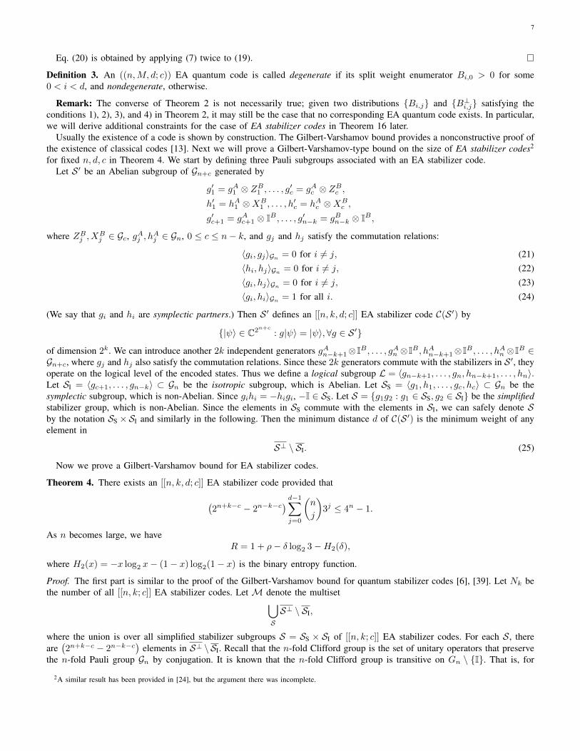
does not depend on c. In Fig. 1,we plot the degenerate and nondegenerate Hamming bounds at d = 9 and c = 3. The two bounds coincide after n = 19. Wehave observed similar behaviors for several values of d and t. Thus we have the following conjecture:

Conjecture 9. The nondegenerate Hamming bound (32) holds for degenerate ((n,M, d; c)) EA quantum codes for n ≥ N(t),where N(t) does not depend on c.

The first few values of N(t) are listed in Table I. Similar results have been observed for data-syndrome codes [26].

t 2 3 4 5 6 7 8 9 10N(t) 9 14 19 24 30 35 40 46 51

TABLE I: Values of N(t) for 2 ≤ t ≤ 10.Recall that Theorem 4 suggests that M can be larger by introducing entanglement assistance. Also the degenerate and

nondegenerate Hamming bounds diverge at low code rate from the above discussion. Consequently, it is likely that EAquantum codes violate the nondegenerate Hamming bound, as evidences have been provided in [46]: A family of degenerate[[n = 4t, 1, 2t+ 1; 1]] EA stabilizer codes for t ≥ 2 has been constructed, which violate (32).

On the other hand, the nondegenerate Hamming bound is valid for quantum codes in the asymptotic case for δ = d/n <1/3 [15], and similarly for EA quantum codes. Then applying (26) to (32), we have the following corollary.

11

Fig. 1: Plots of the degenerate and nondegenerate Hamming bounds at d = 9 and c = 3.

Corollary 10. For any ((n,M, d; c)) EA quantum code with large n,

log2M

n≤ 1 + ρ− δ

2log2 3−H2(

δ

2) + o(1),

where ρ = c/n and δ = d/n < 1/3.

By introducing entanglement assistance, distance can be increased [47]. Again consider the family of [[n = 4t, 1, 2t+ 1; 1]]EA stabilizer codes. These codes have relative distance δ = 0.5, which is beyond the working region of the Hamming bound.

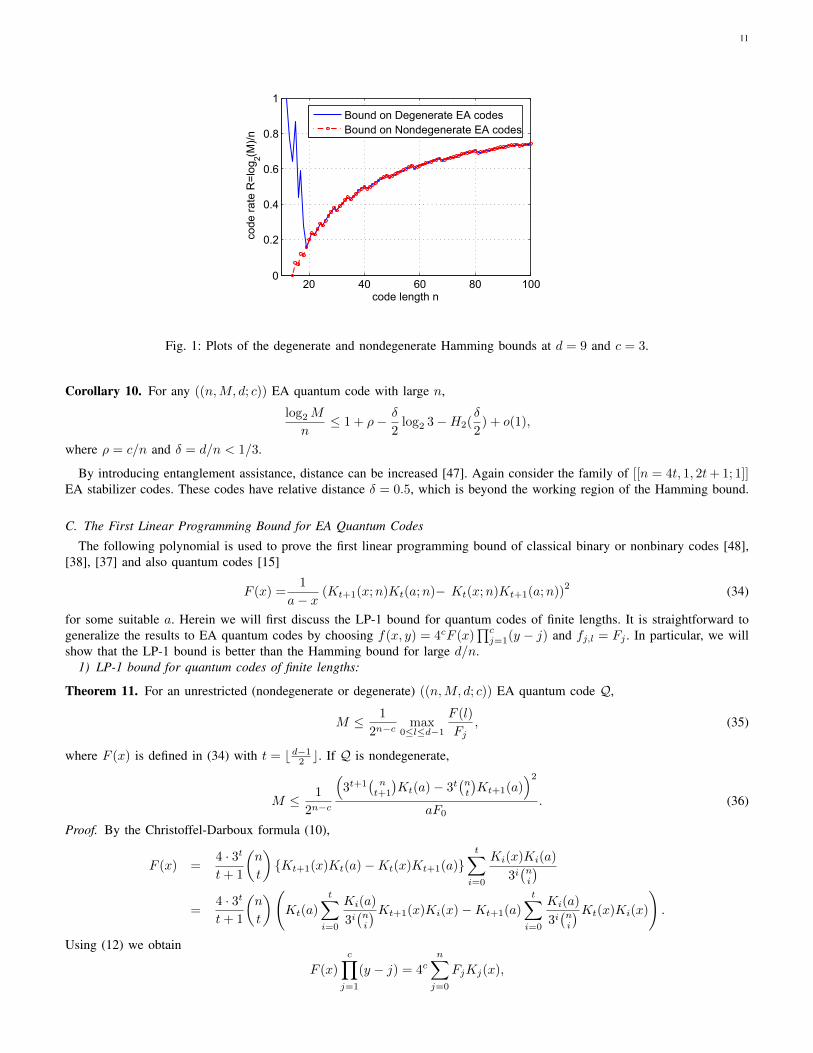
C. The First Linear Programming Bound for EA Quantum Codes

The following polynomial is used to prove the first linear programming bound of classical binary or nonbinary codes [48],[38], [37] and also quantum codes [15]

F (x) =1

a− x(Kt+1(x;n)Kt(a;n)− Kt(x;n)Kt+1(a;n))

2 (34)

for some suitable a. Herein we will first discuss the LP-1 bound for quantum codes of finite lengths. It is straightforward togeneralize the results to EA quantum codes by choosing f(x, y) = 4cF (x)

∏cj=1(y − j) and fj,l = Fj . In particular, we will

show that the LP-1 bound is better than the Hamming bound for large d/n.1) LP-1 bound for quantum codes of finite lengths:

Theorem 11. For an unrestricted (nondegenerate or degenerate) ((n,M, d; c)) EA quantum code Q,

M ≤ 1

2n−cmax

0≤l≤d−1

F (l)

Fj, (35)

where F (x) is defined in (34) with t = bd−12 c. If Q is nondegenerate,

M ≤ 1

2n−c

(3t+1

(nt+1

)Kt(a)− 3t

(nt

)Kt+1(a)

)2aF0

. (36)

Proof. By the Christoffel-Darboux formula (10),

F (x) =4 · 3t

t+ 1

(n

t

){Kt+1(x)Kt(a)−Kt(x)Kt+1(a)}

t∑i=0

Ki(x)Ki(a)

3i(ni

)=

4 · 3t

t+ 1

(n

t

)(Kt(a)

t∑i=0

Ki(a)

3i(ni

)Kt+1(x)Ki(x)−Kt+1(a)

t∑i=0

Ki(a)

3i(ni

)Kt(x)Ki(x)

).

Using (12) we obtain

F (x)

c∏j=1

(y − j) = 4cn∑j=0

FjKj(x),

12

with

Fj =4 · 3t

t+ 1

(n

t

)(Kt(a)

t∑i=0

Ki(a)

3i(ni

) n−j∑s=0

α(j, t+ 1, i, s) −Kt+1(a)

t∑i=0

Ki(a)

3i(ni

) n−j∑s=0

α(j, t, i, s)

). (37)

From (37) it follows that by choosing appropriate a ∈ (rt+1, rt), we can guarantee that Fj ≥ 0. Then we can applyTheorem 5 with f(x, y) = 4cF (x)

∏cj=1(y − j) and fj,l = Fj .

Even for small values of n we have to manipulate by very large numbers during computation of the bound

max0≤j≤d−1

F (j)/Fj .

The values of Krawtchouk polynomials and binomial coefficients in (37) grow very rapidly with n. Though packages like Mapleand Mathematica allow one to operate with very large numbers by increasing the precision of computations, straightforwardcomputations of F (j) and Fj are getting very slow even at relatively small n. The following simple tricks allow to speed upMaple computations significantly.

First, the analysis of (37) shows the limits of summations can be computed more accurately, leading to the equation:

Fj =4 · 3t

t+ 1

(n

t

)Kt(a)

t∑i=0

Ki(a)

3i(ni

) min{n−j,(t+i+1−j)/2}∑s=max{0,(t+i+1−2j)/2,t+1−j}

α(j, t+ 1, i, s)

−Kt+1(a)

t∑i=0

Ki(a)

3i(ni

) min{n−j,(t+i−j)/2}∑s=max{0,(t+i−2j)/2,t+1−j}

α(j, t, i, s)

. (38)

Second, in (38) the two summations over s do not depend on a. So, for given j and i, we can pre-compute and reuse themfor getting Fj for different values of a.

Third, computation of Kt(x) according to (11) is much faster than according to (6).To get a good bound for a particular value of n, we have to optimize the choice of parameters t and a in (34). The following

procedure is used:1. Find the smallest t such that rt < d. In order of doing this, we start with t0 = 3n

4 −d2 −

12

√3d(n− d) and increase t until

Kt(d) < 0.2. Find rt and rt+1.3. Find

aopt = arg mina∈(rt+1,rt)

max0≤j≤d−1

F (j)

Fj. (39)

For example, for n = 50 and d = 15, we have t = 15 and rt+1 ≈ 13.543, rt ≈ 14.510. The behavior of max0≤j≤d−1 F (j)/Fjas a function of a is shown in Fig. 2. In all our computations this function was convex. So, we conjecture that this is alwaysthe case.

Fig. 2: maxj F (j)/Fj as a function of parameter a for n = 50 and d = 15

The analysis of (37) shows that if we fix n and start increasing d, then at a certain moment we will have Fj = 0 for somej ≤ d − 1. For instance, for n = 30 this happens when d ≥ 15 and for n = 60 this happens for d ≥ 25. To overcome this

13

problem one may try to choose larger t so that it is not the first t for which rt < d. We leave this possibility, however, forfuture work. In this work we assume that if Fj = 0, j < d, then LP-1 bound is not applicable.

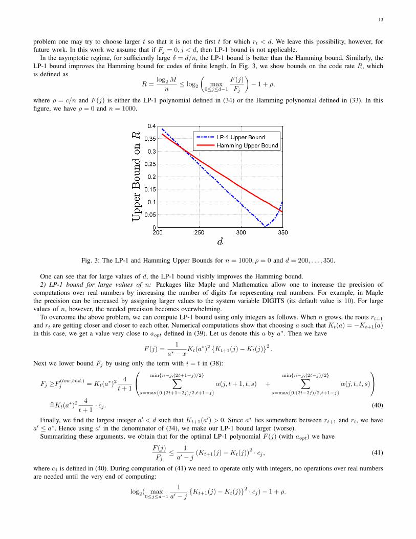
In the asymptotic regime, for sufficiently large δ = d/n, the LP-1 bound is better than the Hamming bound. Similarly, theLP-1 bound improves the Hamming bound for codes of finite length. In Fig. 3, we show bounds on the code rate R, whichis defined as

R =log2M

n≤ log2

(max

0≤j≤d−1

F (j)

Fj

)− 1 + ρ,

where ρ = c/n and F (j) is either the LP-1 polynomial defined in (34) or the Hamming polynomial defined in (33). In thisfigure, we have ρ = 0 and n = 1000.

Fig. 3: The LP-1 and Hamming Upper Bounds for n = 1000, ρ = 0 and d = 200, . . . , 350.

One can see that for large values of d, the LP-1 bound visibly improves the Hamming bound.2) LP-1 bound for large values of n: Packages like Maple and Mathematica allow one to increase the precision of

computations over real numbers by increasing the number of digits for representing real numbers. For example, in Maplethe precision can be increased by assigning larger values to the system variable DIGITS (its default value is 10). For largevalues of n, however, the needed precision becomes overwhelming.

To overcome the above problem, we can compute LP-1 bound using only integers as follows. When n grows, the roots rt+1

and rt are getting closer and closer to each other. Numerical computations show that choosing a such that Kt(a) = −Kt+1(a)in this case, we get a value very close to aopt defined in (39). Let us denote this a by a∗. Then we have

F (j) =1

a∗ − xKt(a

∗)2 {Kt+1(j)−Kt(j)}2 .

Next we lower bound Fj by using only the term with i = t in (38):

Fj ≥F (low.bnd.)j = Kt(a

∗)24

t+ 1

min{n−j,(2t+1−j)/2}∑s=max{0,(2t+1−2j)/2,t+1−j}

α(j, t+ 1, t, s) +

min{n−j,(2t−j)/2}∑s=max{0,(2t−2j)/2,t+1−j}

α(j, t, t, s)

,Kt(a

∗)24

t+ 1· cj . (40)

Finally, we find the largest integer a′ < d such that Kt+1(a′) > 0. Since a∗ lies somewhere between rt+1 and rt, we havea′ ≤ a∗. Hence using a′ in the denominator of (34), we make our LP-1 bound larger (worse).

Summarizing these arguments, we obtain that for the optimal LP-1 polynomial F (j) (with aopt) we have

F (j)

Fj≤ 1

a′ − j(Kt+1(j)−Kt(j))

2 · cj , (41)

where cj is defined in (40). During computation of (41) we need to operate only with integers, no operations over real numbersare needed until the very end of computing:

log2( max0≤j≤d−1

1

a′ − j{Kt+1(j)−Kt(j)}2 · cj)− 1 + ρ.

14

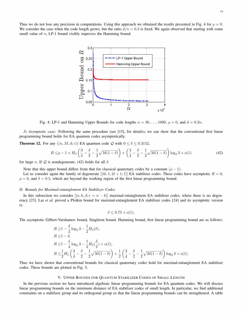
Thus we do not lose any precision in computations. Using this approach we obtained the results presented in Fig. 4 for ρ = 0.We consider the case when the code length grows, but the ratio d/n = 0.3 is fixed. We again observed that starting with somesmall value of n, LP-1 bound visibly improves the Hamming bound.

Fig. 4: LP-1 and Hamming Upper Bounds for code lengths n = 30, . . . , 1000, ρ = 0, and d = 0.3n.

3) Asymptotic case: Following the same procedure (see [15], for details), we can show that the conventional first linearprogramming bound holds for EA quantum codes asymptotically.

Theorem 12. For any ((n,M, d; c)) EA quantum code Q with 0 ≤ δ ≤ 0.3152,

R ≤ρ− 1 +H2

(3

4− δ

2− 1

2

√3δ(1− δ)

)+

(3

4− δ

2− 1

2

√3δ(1− δ)

)log2 3 + o(1) (42)

for large n. If Q is nondegenerate, (42) holds for all δ.

Note that this upper bound differs from that for classical quaternary codes by a constant (ρ− 1).Let us consider again the family of degenerate [[4t, 1, 2t+ 1; 1]] EA stabilizer codes. These codes have asymptotic R = 0,

ρ = 0, and δ = 0.5, which are beyond the working region of the first linear programming bound.

D. Bounds for Maximal-entanglement EA Stabilizer Codes

In this subsection we consider [[n, k, d; c = n − k]] maximal-entanglement EA stabilizer codes, where there is no degen-eracy [23]. Lai et al. proved a Plotkin bound for maximal-entanglement EA stabilizer codes [24] and its asymptotic versionis:

δ ≤ 0.75 + o(1).

The asymptotic Gilbert-Varshamov bound, Singleton bound, Hamming bound, first linear programming bound are as follows:

R ≥1− δ

2log2 3− 1

2H2(δ),

R ≤1− δ,

R ≤1− δ

4log2 3− 1

2H2(

δ

2) + o(1),

R ≤1

2H2

(3

4− δ

2− 1

2

√3δ(1− δ)

)+

1

2

(3

4− δ

2− 1

2

√3δ(1− δ)

)log2 3 + o(1).

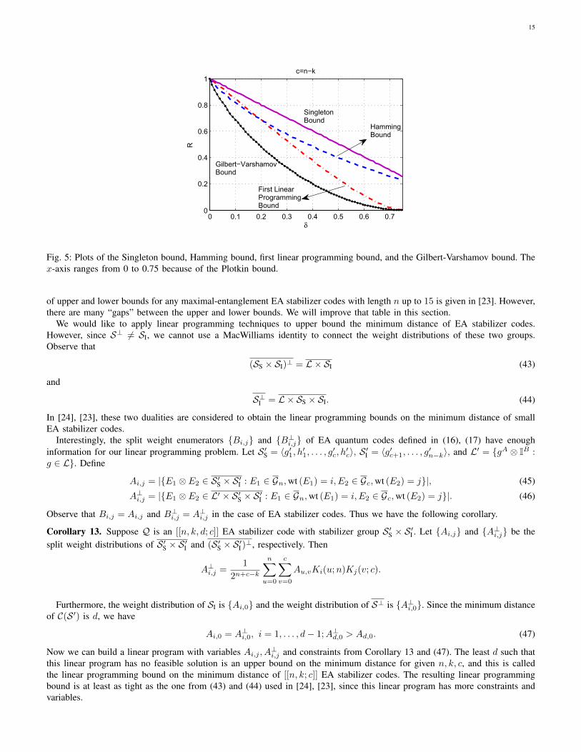
Thus we have shown that conventional bounds for classical quaternary codes hold for maximal-entanglement EA stabilizercodes. These bounds are plotted in Fig. 5.

V. UPPER BOUNDS FOR QUANTUM STABILIZER CODES OF SMALL LENGTH

In the previous section we have introduced algebraic linear programming bounds for EA quantum codes. We will discusslinear programming bounds on the minimum distance of EA stabilizer codes of small length. In particular, we find additionalconstraints on a stabilizer group and its orthogonal group so that the linear programming bounds can be strengthened. A table

15

Fig. 5: Plots of the Singleton bound, Hamming bound, first linear programming bound, and the Gilbert-Varshamov bound. Thex-axis ranges from 0 to 0.75 because of the Plotkin bound.

of upper and lower bounds for any maximal-entanglement EA stabilizer codes with length n up to 15 is given in [23]. However,there are many “gaps” between the upper and lower bounds. We will improve that table in this section.

We would like to apply linear programming techniques to upper bound the minimum distance of EA stabilizer codes.However, since S⊥ 6= SI, we cannot use a MacWilliams identity to connect the weight distributions of these two groups.Observe that

(SS × SI)⊥ = L × SI (43)

and

S⊥I = L × SS × SI. (44)

In [24], [23], these two dualities are considered to obtain the linear programming bounds on the minimum distance of smallEA stabilizer codes.

Interestingly, the split weight enumerators {Bi,j} and {B⊥i,j} of EA quantum codes defined in (16), (17) have enoughinformation for our linear programming problem. Let S ′S = 〈g′1, h′1, . . . , g′c, h′c〉, S ′I = 〈g′c+1, . . . , g

′n−k〉, and L′ = {gA ⊗ IB :

g ∈ L}. Define

Ai,j = |{E1 ⊗ E2 ∈ S ′S × S ′I : E1 ∈ Gn,wt (E1) = i, E2 ∈ Gc,wt (E2) = j}|, (45)

A⊥i,j = |{E1 ⊗ E2 ∈ L′ × S ′S × S ′I : E1 ∈ Gn,wt (E1) = i, E2 ∈ Gc,wt (E2) = j}|. (46)

Observe that Bi,j = Ai,j and B⊥i,j = A⊥i,j in the case of EA stabilizer codes. Thus we have the following corollary.

Corollary 13. Suppose Q is an [[n, k, d; c]] EA stabilizer code with stabilizer group S ′S × S ′I . Let {Ai,j} and {A⊥i,j} be thesplit weight distributions of S ′S × S ′I and (S ′S × S ′I )⊥, respectively. Then

A⊥i,j =1

2n+c−k

n∑u=0

c∑v=0

Au,vKi(u;n)Kj(v; c).

Furthermore, the weight distribution of SI is {Ai,0} and the weight distribution of S⊥ is {A⊥i,0}. Since the minimum distanceof C(S ′) is d, we have

Ai,0 = A⊥i,0, i = 1, . . . , d− 1;A⊥d,0 > Ad,0. (47)

Now we can build a linear program with variables Ai,j , A⊥i,j and constraints from Corollary 13 and (47). The least d such thatthis linear program has no feasible solution is an upper bound on the minimum distance for given n, k, c, and this is calledthe linear programming bound on the minimum distance of [[n, k; c]] EA stabilizer codes. The resulting linear programmingbound is at least as tight as the one from (43) and (44) used in [24], [23], since this linear program has more constraints andvariables.

16

A. Additional Constraints on the Weight Enumerator Associated with an Non-Abelian Pauli Subgroup

Rains introduced the idea of shadow enumerators to obtain additional constraints in the linear program of quantum codes [27].The shadow Sh(V) of a group V(⊆ Gn) is the set

{E ∈ Gn : 〈E, g〉Gn = wt (g) mod 2, ∀g ∈ V}.

If V is Abelian, Rains showed that

WSh(V)(x, y) =1

|V|WV(x+ 3y, y − x), (48)

where WV(x, y) and WSh(V)(x, y) are the weight enumerators of V and Sh(V), respectively [27]. For an EA stabilizer code,the isotropic subgroup SI is Abelian. Thus

WSh(SI)(x, y) =1

|SI|WSI(x+ 3y, y − x).

Recall that {Ai,0} is the weight distribution of SI. This impliesn∑

w′=0

(−1)w′Aw′,0Kw(w′;n) ≥ 0, i = 0, . . . , n. (49)

However, the situation is more complicated when V is not Abelian, which is the case of the simplified stabilizer groupS = SS × SI and its orthogonal group. Herein we derive additional constraints for an non-Abelian Pauli subgroup.

Suppose V ⊂ Gn is non-Abelian and V can be decomposed as V = VS × VI, where VS = 〈g1, h1, . . . , gc, hc〉 and VI =〈gc+1, . . . , gc+r〉 for some c such that the commutation relations (21)-(24) hold [49]. We categorize different V’s into thefollowing three types:

I. All the generators of V are of even weight.II. wt (gc+1) is odd and all the other generators of VI and VS are of even weight.

III. wt (g1) and wt (h1) are odd and all the other generators of VS and VI are of even weight.For convenience, we have the following lemma, which can be easily verified.

Lemma 14. For g, h ∈ Gn,wt (gh) ≡ wt (g) + wt (h) + 〈g, h〉Gn mod 2.

This lemma shows that the weight of the product of two operators depends on their inner product.

Lemma 15. Suppose V = VS ×VI, where VS = 〈g1, h1, . . . , gc, hc〉 and VI = 〈gc+1, . . . , gc+r〉 for some c such that (21)-(24)hold. Then the generators are of type I, II, or III.

Proof. Suppose VI contains some elements of odd weight, say gc+1 without loss of generality. If gj or hj is of odd weightfor j 6= c+ 1, it is replaced by gjgc+1 or hjgc+1, which is of even weight by (21), (23), and Lemma 14. Eqs. (21)-(24) holdfor the new set of generators. This is type II.

Next, suppose VI contains no elements of odd weight. Consider the generators of VS. We know that VS has some elementsof odd weight, because one of g1, h1, and g1h1 must be of odd weight. Assume g1 is of odd weight without loss of generality.If gi is of odd weight for i = 2, . . . , c, we replace it with gigc+1, which is of even weight by (21) and Lemma 14. Noticethat h1 has to be replaced by h1hi at the same time to maintain the commutation relation in (23). Thus wt (g1) is odd andwt (g2) , . . . ,wt (gc) are even. If hi has odd weight for i = 2, . . . , c, we replace it with hig1, which is of even weight by (22)and Lemma 14. Similarly, h1 has to be replaced by h1gi to maintain the commutation relation in (22). Therefore, we canassume h2, . . . , hc are of even weight.

It remains to check whether h1 is of odd weight or not. If wt (h1) is odd, this is type III. If wt (h1) is even, we replace g1with g1h1, which is of even weight by Eq. (24) and Lemma 14. This case is type I.

Suppose V ⊂ Gn is generated by c pairs of symplectic partners and r isotropic generators of type i. Let N eveni (c, r) and

N oddi (c, r) be the number of elements in V of even and odd weight, respectively. Below we derive formulas for these two

numbers for the three types of generators in Lemma 15.

17

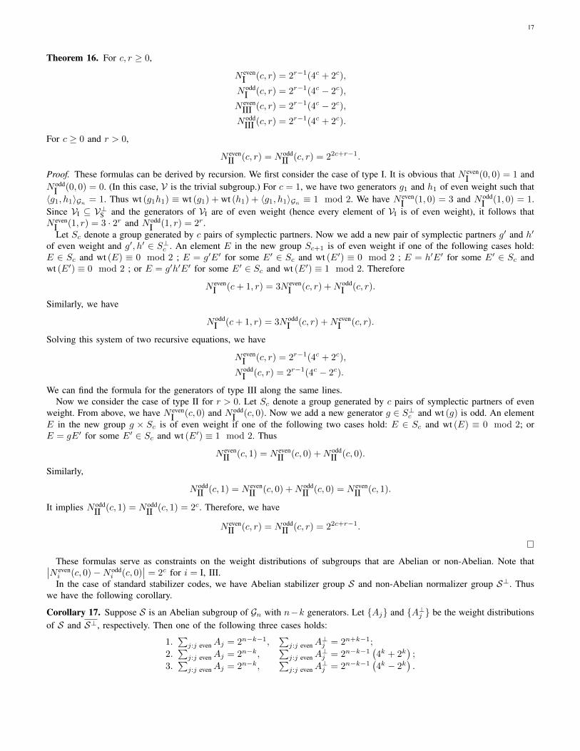
Theorem 16. For c, r ≥ 0,

N evenI (c, r) = 2r−1(4c + 2c),

N oddI (c, r) = 2r−1(4c − 2c),

N evenIII (c, r) = 2r−1(4c − 2c),

N oddIII (c, r) = 2r−1(4c + 2c).

For c ≥ 0 and r > 0,

N evenII (c, r) = N odd

II (c, r) = 22c+r−1.

Proof. These formulas can be derived by recursion. We first consider the case of type I. It is obvious that N evenI (0, 0) = 1 and

N oddI (0, 0) = 0. (In this case, V is the trivial subgroup.) For c = 1, we have two generators g1 and h1 of even weight such that〈g1, h1〉Gn = 1. Thus wt (g1h1) ≡ wt (g1) + wt (h1) + 〈g1, h1〉Gn ≡ 1 mod 2. We have N even

I (1, 0) = 3 and N oddI (1, 0) = 1.

Since VI ⊆ V⊥S and the generators of VI are of even weight (hence every element of VI is of even weight), it follows thatN even

I (1, r) = 3 · 2r and N oddI (1, r) = 2r.

Let Sc denote a group generated by c pairs of symplectic partners. Now we add a new pair of symplectic partners g′ and h′

of even weight and g′, h′ ∈ S⊥c . An element E in the new group Sc+1 is of even weight if one of the following cases hold:E ∈ Sc and wt (E) ≡ 0 mod 2 ; E = g′E′ for some E′ ∈ Sc and wt (E′) ≡ 0 mod 2 ; E = h′E′ for some E′ ∈ Sc andwt (E′) ≡ 0 mod 2 ; or E = g′h′E′ for some E′ ∈ Sc and wt (E′) ≡ 1 mod 2. Therefore

N evenI (c+ 1, r) = 3N even

I (c, r) +N oddI (c, r).

Similarly, we have

N oddI (c+ 1, r) = 3N odd

I (c, r) +N evenI (c, r).

Solving this system of two recursive equations, we have

N evenI (c, r) = 2r−1(4c + 2c),

N oddI (c, r) = 2r−1(4c − 2c).

We can find the formula for the generators of type III along the same lines.Now we consider the case of type II for r > 0. Let Sc denote a group generated by c pairs of symplectic partners of even

weight. From above, we have N evenI (c, 0) and N odd

I (c, 0). Now we add a new generator g ∈ S⊥c and wt (g) is odd. An elementE in the new group g × Sc is of even weight if one of the following two cases hold: E ∈ Sc and wt (E) ≡ 0 mod 2; orE = gE′ for some E′ ∈ Sc and wt (E′) ≡ 1 mod 2. Thus

N evenII (c, 1) = N even

II (c, 0) +N oddII (c, 0).

Similarly,

N oddII (c, 1) = N even

II (c, 0) +N oddII (c, 0) = N even

II (c, 1).

It implies N oddII (c, 1) = N odd

II (c, 1) = 2c. Therefore, we have

N evenII (c, r) = N odd

II (c, r) = 22c+r−1.

These formulas serve as constraints on the weight distributions of subgroups that are Abelian or non-Abelian. Note that∣∣N eveni (c, 0)−N odd

i (c, 0)∣∣ = 2c for i = I, III.

In the case of standard stabilizer codes, we have Abelian stabilizer group S and non-Abelian normalizer group S⊥. Thuswe have the following corollary.

Corollary 17. Suppose S is an Abelian subgroup of Gn with n−k generators. Let {Aj} and {A⊥j } be the weight distributionsof S and S⊥, respectively. Then one of the following three cases holds:

1.∑j:j even Aj = 2n−k−1,

∑j:j even A

⊥j = 2n+k−1;

2.∑j:j even Aj = 2n−k,

∑j:j even A

⊥j = 2n−k−1

(4k + 2k

);

3.∑j:j even Aj = 2n−k,

∑j:j even A

⊥j = 2n−k−1

(4k − 2k

).

18

B. Linear Program for EA Stabilizer Codes

Now we provide a linear program for EA stabilizer codes in this subsection. Let n, k, d, c be integers. Define integer variables

Ai,j , A⊥i,j , i = 0, . . . , n, j = 0, . . . , c.

The following constraints are from Theorem 2, Corollary 13, Eq. (49), and Theorem 16:

A0,0 = A⊥0,0 = 1, A⊥i,j ≥ Ai,j ≥ 0;

Ai,0 = A⊥i,0, i = 1, . . . , d− 1;A0,j = A⊥0,j = 0, j = 1, . . . , c;n∑

w=0

Aw,0 = 2n−k−c,

n∑w=0

c∑w′=0

Aw,w′ = 2n−k+c,

n∑w=0

A⊥w,0 = 2n+k−c,

n∑w=0

c∑w′=0

A⊥w,w′ = 2n+k+c;

A⊥i,j =1

2n+c−k

n∑u=0

c∑v=0

Au,vKi(u;n)Kj(v; c);

n∑w′=0

(−1)w′Aw′,0Kw(w′;n) ≥ 0, i = 0, . . . , n;

( ∑w:even

∑w′

Aw,w′ = N eveni (c, n− k − c), for i = I or III,

∑w:even

A⊥w,0 = N eveni (k, n− k − c), for i = I or III,

∑w:even

∑w′

A⊥w,w′ = N eveni (k + c, n− k − c), for i = I or III, and

∑w:even

Aw,0 = 2n−k−c

)

or

( ∑w:even

∑w′

Aw,w′ = N evenII (c, n− k − c),

∑w:even

A⊥w,0 = N evenII (k, n− k − c),

∑w:even

∑w′

A⊥w,w′ = N evenII (k + c, n− k − c), and

∑w:even

Aw,0 = 2n−k−c−1

).

If there is no solution to the integer program with variables Ai,j , A⊥i,j and the above constraints for given n, k, d, and c, thenthere is no [[n, k, d; c]] EA stabilizer code.

We can introduce additional constraints from MacWilliams identities for general split weight enumerators [36]. In thefollowing, we use the notation in [36]. Let HG1

be the complex Hilbert space with an orthonormal basis |I〉, |X〉, |Y 〉, |Z〉.Let HGn

= H⊗nG1. Then S ⊂ Gn has an exact weight generator

gES =∑g∈S

|g〉 ∈ HGn.

The MacWilliams identity says that

gES⊥ =1

|S|F⊗ngES , (50)

where F is the Fourier transform operator on HG1and its matrix representation in the ordered basis |I〉, |X〉, |Y 〉, |Z〉 is

F =

1 1 1 11 1 −1 −11 −1 1 −11 −1 −1 1

. (51)

Let γ : HGn→ C be a linear functional. Then applying γ to (50), we have the MacWilliams identities for general split weight

enumerators defined by γ. (See [36] for more details.) For example, let

γH(x, y) = x〈I|+∑

α∈{X,Y,Z}

y〈α|,

where x, y ∈ C. Then the general Hamming weight enumerator of S and its MacWilliams identity are defined by γ⊗nH (x, y).The split weight enumerators (45), (46) are defined by γ⊗nH (x, y)⊗ γ⊗cH (u, v).

In general, an arbitrary γ and its induced MacWilliams identity will lead to more constraints on the coefficients of S andS⊥. However, these general split weight enumerators usually introduce too many variables to solve in a computer program.If we know more about a stabilizer group, we can design an effective γ. In [7], the idea of refined weight enumerator is

19

introduced when S is known to have an element of weight u. Let

γre(y0, y1, y2) = y0〈I|+ y1〈X|+∑

α∈{Y,Z}

y2〈α|.

Then a refined weight enumerator is defined as

γ⊗n−uH (x0, x1)⊗ γ⊗ure (y0, y1, y2)gES =∑i,j,l

Ai,j,lxn−u−i0 xi1y

u−j−l0 yj1y

l2. (52)

Suppose {Ai} is the weight distribution of S. Then

Aw =∑

i,j,l:i+j+l=w

Ai,j,l.

Without loss of generality, we may assume S has the element I⊗n−u ⊗X⊗u of weight u. Since S is Abelian, we must haveAi,j,l = 0 for l 6= 0 mod 2. Similar constraints can be found for the distribution A⊥i,j,l of S⊥. From (50), we have additionalconstraints from the MacWilliams identities on Ai,j,l and A⊥i,j,l.

Next we use Mathematica [50] to see if the integer program has a feasible solution for some parameters. Since Mathematicais a symbolic manipulation program, the results are reliable.

Example 1. (Nonexistence of [[27,15,5]] quantum codes.) In the case of c = 0, SS is trivial and it reduces to the case ofstandard stabilizer codes. Solving the linear program for stabilizer codes [7] with additional constraints from Corollary 17,we found that a [[27, 15, 5]] stabilizer code, if it exists, must have S⊥ generated by type III generators and the only possibleweight distribution of S is

A0 = 1, A16 = 81, A18 = 1800, A22 = 1944, A24 = 270,

and Aw = 0, otherwise.Using refined weight enumerators with respect to u = 24, we have additional constraints from the MacWilliams identities

for the refined weight enumerators, which produce a linear program with no feasible solution. Thus we improved the quantumcode table at n = 27, k = 15 [51].

Example 2. (Nonexistence of [[28,14,6]] quantum codes.) We found that a [[28, 14, 6]] stabilizer code, if it exists, must haveS⊥ generated by type I generators and the only possible weight distribution of S is

A0 = 1, A16 = 189, A18 = 5040, A22 = 9072, A24 = 1890, A28 = 192,

and Aw = 0, otherwise. This implies that a [[28, 14, 6]] code must be nondegenerate. By the propagation rule that the existenceof a nondegenerate [[n, k, d]] code implies the existence of an [[n − 1, k + 1, d − 1]] code [7, Theorem 6], if we have anondegenerate [[28, 14, 6]] code, there is a [[27, 15, 5]] code. However, the existence of a [[27, 15, 5]] code has been excludedin Example 1. Thus there is no [[28, 14, 6]] code.

Example 3. Similarly, a [[23, 1, 9]] stabilizer code, if it exists, must have S⊥ generated by type III generators and the onlypossible weight distribution of S is

A0 = 1, A10 = 10626, A12 = 78246, A14 = 478170, A16 = 1245519, A18 = 1562022, A20 = 733194, A22 = 86526

and Aw = 0, otherwise. Unfortunately, we do not know how to exclude these possibilities. Some other techniques are needed.We also found that several quantum codes, such as the parameters [[14, 3, 5]], [[17, 3, 6]], [[17, 6, 5]], [[19, 5, 6]], [[21, 7, 6]],

[[23, 3, 8]] and so on, must have S⊥ with generators of type II, if they exist.

Next we consider maximal-entanglement EA stabilizer codes, where SI is trivial, in the following example.

Example 4. Solving the integer program, we eliminate the existence of [[4, 2, 3; 2]], [[5, 3, 3; 2]], [[5, 2, 4; 3]], [[6, 3, 4; 3]],[[9, 2, 7; 7]], [[10, 2, 8; 8]], [[10, 3, 7; 7]], [[11, 3, 8; 8]], [[14, 2, 11; 12]], [[14, 3, 10; 11]], [[15, 2, 12; 13]], [[15, 3, 11; 12]], [[15, 8, 7; 7]],[[15, 9, 6; 6]],[[16, 4, 11; 12]], [[17, 4, 12; 13]],[[20, 3, 15; 17]] EA stabilizer codes. The constraints from Theorem 16 are effectivein the case of maximal-entanglement EA stabilizer codes.

C. Nonexistence of [[5, 3, 3; 2]], [[4, 2, 3; 2]], [[5, 2, 4; 3]], and [[6, 3, 4; 3]] EA stabilizer Codes

A general method to prove or disprove the existence of a code of certain parameters is to use computer search over allpossibilities. It is applicable when the search space is small. Here we consider a general form of the check matrix of quantumcodes and use computer search to rule out the existence of some small EA stabilizer codes.

20

The parity-check matrix corresponding to a simplified stabilizer group S = 〈g1, . . . , gn−k, h1, . . . , hc〉 is defined as

H =

τ(g1)...

τ(gn−k)τ(h1)

...τ(hc)

with rank

(HΛ2nH

T)

= 2c [52], where the superscript T means transpose and Λ2n =

[0n×n InIn 0n×n

]. Recall that τ : Gn →

Z2n2 is defined in (2).Theorem 2 in Ref. [53] states that a check matrix of a nondegenerate [[n, k, d; c]] code can be transformed into a standard

form H =

Is A D 00 C Is B0 E 0 F

, where Is is the s × s identity matrix and s ≥ d − 1. Since a maximal-entanglement EA

stabilizer code is nondegenerate, we can construct a check matrix in that form. The check matrix of an [[5, 3, 3; 2]] code, if itexists, can be written as

H = [HX |HZ ] =

1 0 ∗ ∗ ∗ 0 0 ∗ ∗ ∗0 1 ∗ ∗ ∗ 0 0 ∗ ∗ ∗0 0 ∗ ∗ ∗ 1 0 ∗ ∗ ∗0 0 ∗ ∗ ∗ 0 1 ∗ ∗ ∗

,where a “ ∗ ” can be 0 or 1. The error syndromes of single-qubit Pauli errors Xi and Zj are the i-th column and j-th columnof HX and HZ , respectively. If the syndromes of Xi and Zi are sxi , and szi , respectively, then the syndrome of Yi is sxi + szi .Our goal is to fill in the missing columns such that rank(HΛHT ) = 4 and each single-qubit Pauli error has a unique errorsyndrome, since the minimum distance is three [54].

Let the integer number corresponding to a column vector [a0 a1 a2 a3]T be∑3i=0 a023−i. The columns 8, 4, 2, and 1 have

appeared in the above standard form, and hence so have the columns 10 and 5 (the syndromes of Y1 and Y2). The remainingcandidates are 3, 6, 7, 9, 11, 12, 13, 14, and 15. We group these columns as follows:

G1 : 3, 12, 15; G2 : 3, 13, 14; G3 : 6, 9, 15;G4 : 6, 11, 13; G5 : 7, 9, 14; G6 : 7, 11, 12.

The three columns in any one of the six groups are candidates of the syndromes of Xi, Zi, and Yi for a fixed i. We furtherdivide these six groups into two non-overlapping sets: S1 = {G1, G4, G5} and S2 = {G2, G3, G6}. To fill in the missingcolumns of H , we first choose a set Sj , and then choose two columns from each of the three groups in Sj . Consequently, thetotal number of candidates for H is

2× (

(3

2

)× 2!)3 = 432.

We verified that none of them has rank(HΛHT ) = 4. Hence there is no [[5, 3, 3; 2]] EA stabilizer code.The same technique shows that there are no [[4, 2, 3; 2]], [[5, 2, 4; 3]], or [[6, 3, 4; 3]] EA stabilizer codes.

D. Nonexistence of other EA stabilizer Codes

A maximal-entanglement EA code can also be uniquely defined by a logical group L. Like the check matrix, we can definea logical matrix L corresponding to L with

rank(LΛ2nLT ) = 2k.

Thus maximal-entanglement EA codes are a special case of classical additive quaternary code [7], [47].

Lemma 18. An upper bound on the minimum distance of a classical (n, 22k) additive quaternary code is an upper bound onthe minimum distance of an [[n, k;n− k]] EA stabilizer code.

A table of upper bounds on the minimum distance of additive quaternary codes for length n ≤ 13 is given in [55], [56].From that table, we learn that there are no [[11, 4, 7; 7]], [[12, 5, 7; 7]], [[12, 7, 5; 5]], [[13, 6, 7; 7]], [[13, 7, 6; 6]], or [[13, 8, 5; 5]]EA stabilizer codes. As pointed out in [28], there is no [[15, 5, 9; 10]] EA stabilizer code since there is no (15, 210, 9) additivequaternary code [57].

Lemma 19. An upper bound on the minimum distance of a classical (n, 22k) additive quaternary code is an upper bound onthe minimum distance of an (n + 1, 22(k+1)) additive quaternary code, and hence an upper bound on the minimum distanceof an [[n+ 1, k + 1;n− k]] EA stabilizer code.

21

n\k 1 2 3 4 5 6 7 8 93 3 24 3 2 15 5 3 2 26 5 4 3 2 17 7 5 4 3 2 28 7 6 5 4 3 2 19 9 6 6 5 4 3 2 2

10 9 7 6 6 5 4 3 2 111 11 8 7 6 6 5 4 3 212 11 9 8 7 6 5-6 4 4 313 13 10 9 8 7 6 5 4 414 13 10 9 8 7-8 6-7 6 5 415 15 11 10 9-10 8 7-8 6-7 6 516 15 12 11 10 9 8 7-8 6-7 617 17 13 12 11 9-10 8-9 7-8 7-8 6-718 17 14 13 11-12 10-11 9-10 8-9 8-9 7-819 19 14 13-14 12-13 11 10-11 8-9 8-9 820 19 15 14 13 12 11-12 9-10 8-10 8-9n\k 10 11 12 13 14 15 16 17 1811 212 2 113 3 2 214 4 3 2 115 4 4 3 2 216 5 4 4 3 2 117 6 5 4 3-4 3 2 218 6-7 5-6 5 4 3 3 2 119 7 6-7 5-6 5 4 3 3 2 220 7-8 6-7 6-7 5-6 5 4 3 2 2

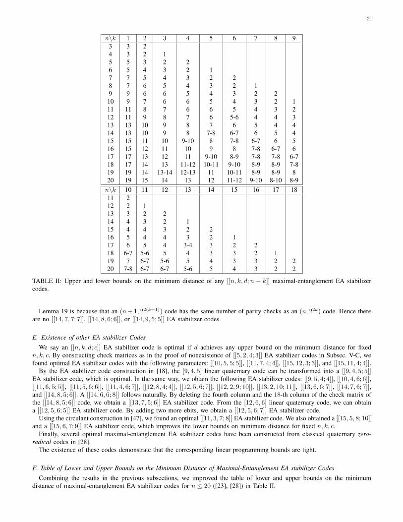
TABLE II: Upper and lower bounds on the minimum distance of any [[n, k, d;n − k]] maximal-entanglement EA stabilizercodes.

Lemma 19 is because that an (n+ 1, 22(k+1)) code has the same number of parity checks as an (n, 22k) code. Hence thereare no [[14, 7, 7; 7]], [[14, 8, 6; 6]], or [[14, 9, 5; 5]] EA stabilizer codes.

E. Existence of other EA stabilizer Codes

We say an [[n, k, d; c]] EA stabilizer code is optimal if d achieves any upper bound on the minimum distance for fixedn, k, c. By constructing check matrices as in the proof of nonexistence of [[5, 2, 4; 3]] EA stabilizer codes in Subsec. V-C, wefound optimal EA stabilizer codes with the following parameters: [[10, 5, 5; 5]], [[11, 7, 4; 4]], [[15, 12, 3; 3]], and [[15, 11, 4; 4]].

By the EA stabilizer code construction in [18], the [9, 4, 5] linear quaternary code can be transformed into a [[9, 4, 5; 5]]EA stabilizer code, which is optimal. In the same way, we obtain the following EA stabilizer codes: [[9, 5, 4; 4]], [[10, 4, 6; 6]],[[11, 6, 5; 5]], [[11, 5, 6; 6]], [[11, 4, 6; 7]], [[12, 8, 4; 4]], [[12, 5, 6; 7]], [[12, 2, 9; 10]], [[13, 2, 10; 11]], [[13, 6, 6; 7]], [[14, 7, 6; 7]],and [[14, 8, 5; 6]]. A [[14, 6, 6; 8]] follows naturally. By deleting the fourth column and the 18-th column of the check matrix ofthe [[14, 8, 5; 6]] code, we obtain a [[13, 7, 5; 6]] EA stabilizer code. From the [12, 6, 6] linear quaternary code, we can obtaina [[12, 5, 6; 5]] EA stabilizer code. By adding two more ebits, we obtain a [[12, 5, 6; 7]] EA stabilizer code.

Using the circulant construction in [47], we found an optimal [[11, 3, 7; 8]] EA stabilizer code. We also obtained a [[15, 5, 8; 10]]and a [[15, 6, 7; 9]] EA stabilizer code, which improves the lower bounds on minimum distance for fixed n, k, c.

Finally, several optimal maximal-entanglement EA stabilizer codes have been constructed from classical quaternary zero-radical codes in [28].

The existence of these codes demonstrate that the corresponding linear programming bounds are tight.

F. Table of Lower and Upper Bounds on the Minimum Distance of Maximal-Entanglement EA stabilizer Codes

Combining the results in the previous subsections, we improved the table of lower and upper bounds on the minimumdistance of maximal-entanglement EA stabilizer codes for n ≤ 20 ([23], [28]) in Table II.

22

VI. DISCUSSION

We have discussed general EA quantum codes, including nonadditive codes, and proposed their algebraic linear programmingbounds, including Singleton-type, Hamming-type, and the first-linear-programming-type bounds. The degenerate and nonde-generate bounds differ for some δ when degeneracy exists. It is known that degenerate EA stabilizer codes can violate the(nondegenerate) Hamming bound. Can we construct such a family of EA stabilizer codes with R > 0? Another interestingquestion is: are there families of degenerate [[n, k, d; c]] EA quantum codes with R > 0, ρ > 0 and 1/3 < δ < 0.75 thatviolate the conventional first linear programming bound? We can also consider the case of imperfect ebits, which should besimilar to the study in [26]. Finally, these results could be strengthened in the case of linear EA stabilizer codes [58], [59].

We provided a refined Singleton bound for EA quantum codes that works for d > (n+ 2)/2; however, it is not monotonicand may not fully characterize the case of large c. A better Singleton bound for EA stabilizer codes with d > (n + 2)/2remains open.

In the setting of usual EA quantum codes, it is assumed that Bob’s qubits are error-free. Thus we chose in Theorem 5 apolynomial of the form

f(x, y) = F (x)

c∏j=1

(y − j),

where F (x) is a polynomial that is used to derive a certain upper bound for general stabilizer codes. The case that Bob’squbits are imperfect [53] can be developed similarly to the split bounds for data-syndrome codes [26], where two types oferrors are considered on two disjoint sets of locations.

The linear programming bounds for small quantum codes are improved. The additional constraints in Theorem 16 areespecially effective for maximal-entanglement EA stabilizer codes, where the generators of a symplectic subgroup or a logicalgroup are of type I or type III. However, they are not that helpful in the case of standard stabilizer codes, where the normalizergroups often have weight distributions of type II. It is possible that the linear programming bounds for standard stabilizercodes can be improved for n ≥ 30.

The EA stabilizer code table in [23] has been significantly improved. Most of the check matrices of the EA stabilizer codesconstructed in this article are omitted because of limited space. All of the gaps between the lower bound and upper bound inTable II are now closed for d ≤ 5 or n ≤ 8. The grouping techniques used in [56] may be generalized to find upper boundson classical additive quaternary codes for n = 15 to 20, which can be used as bounds on maximal-entanglement EA stabilizercodes by Lemma 18.

Other types of split weight enumerators can be introduced into the linear programm for EA stabilizer codes. However,they usually induce too many variables so that the integer program is untraceable when n becomes large. The refined weightenumerator (52) has already introduced too many variables for large n.

The method used in Subsec. V-C is difficult to apply for larger codes because the computational complexity growsexponentially. Perhaps we can construct standard stabilizer codes using this grouping method together with Theorem 2 in [53].

The approach here can be applied to other type of quantum codes, for example, the data-syndrome quantum codes [60],[26], [61], which are codes in the space Fn4 ×Fm2 . Split weight enumerators for these codes can be derived easily. We can alsoapply these techniques to other asymmetric quantum codes.

ACKNOWLEDGMENT

We thank Todd Brun for helpful discussion. We are grateful to Markus Grassl for his comments and suggestions that helpto improve this paper.

REFERENCES

[1] P. W. Shor, “Scheme for reducing decoherence in quantum computer memory,” Phys. Rev. A, vol. 52, no. 4, pp. 2493–2496, 1995.[2] A. Ekert and C. Macchiavello, “Quantum error-correction for communication,” Phys. Rev. Lett., vol. 77, no. 12, pp. 2585–2588, 1996.[3] E. Knill and R. Laflamme, “A theory of quantum error-correcting codes,” Phys. Rev. A, vol. 55, no. 2, pp. 900–911, 1997.[4] A. M. Steane, “Multiple particle interference and quantum error correction,” Proc. R. Soc. London A, vol. 452, pp. 2551–2576, 1996.[5] D. Gottesman, “Stabilizer codes and quantum error correction,” Ph.D. dissertation, California Institute of Technology, Pasadena, CA, 1997.[6] A. R. Calderbank, E. M. Rains, P. W. Shor, and N. J. A. Sloane, “Quantum error correction and orthogonal geometry,” Phys. Rev. Lett., vol. 78, no. 3,

pp. 405–408, 1997.[7] ——, “Quantum error correction via codes over GF (4),” IEEE Trans. Inf. Theory, vol. 44, no. 4, pp. 1369–1387, 1998.[8] M. A. Nielsen and I. L. Chuang, Quantum Computation and Quantum Information. Cambridge, UK: Cambridge University Press, 2000.[9] A. E. Ashikhmin, A. M. Barg, E. Knill, and S. N. Litsyn, “Quantum error detection .I. statement of the problem,” IEEE Trans. Inf. Theory, vol. 46,

no. 3, pp. 778–788, May 2000.[10] ——, “Quantum error detection .II. bounds,” IEEE Trans. Inf. Theory, vol. 46, no. 3, pp. 789–800, May 2000.[11] F. Gaitan, Quantum error correction and fault tolerant quantum computing. Boca Raton, FL: CRC Press, 2008.[12] D. A. Lidar and T. A. Brun, Eds., Quantum Error Correction. Cambridge University Press, October 2013.[13] F. J. MacWilliams and N. J. A. Sloane, The Theory of Error-Correcting Codes. Amsterdam, The Netherlands: North-Holland, 1977.[14] P. Delsarte, “An algebraic approach to the association schemes of coding theory,” Philips Res. Rep. Suppl., vol. 10, 1973.[15] A. Ashikhmin and S. Litsyn, “Upper bounds on the size of quantum codes,” IEEE Trans. Inf. Theory, vol. 45, no. 4, pp. 1206 – 1215, 1999.[16] P. Shor and R. Laflamme, “Quantum analog of the MacWilliams identities for classical coding theory,” Phys. Rev. Lett., vol. 78, no. 8, pp. 1600–1602,

Feb 1997.

23

[17] E. M. Rains, “Quantum weight enumerators,” IEEE Trans. Inf. Theory, vol. 44, no. 4, pp. 1388 – 1394, 1995.[18] T. A. Brun, I. Devetak, and M.-H. Hsieh, “Correcting quantum errors with entanglement,” Science, vol. 314, pp. 436–439, 2006.[19] M.-H. Hsieh, T. A. Brun, and I. Devetak, “Entanglement-assisted quantum quasi-cyclic low-density parity-check codes,” Phys. Rev. A, vol. 79, p. 032340,

2009.[20] M.-H. Hsieh, W.-T. Yen, and L.-Y. Hsu, “High performance entanglement-assisted quantum LDPC codes need little entanglement,” IEEE Trans. Inf.

Theory, vol. 57, no. 3, pp. 1761–1769, 2011.[21] Y. Fujiwara, D. Clark, P. Vandendriessche, M. De Boeck, and V. D. Tonchev, “Entanglement-assisted quantum low-density parity-check codes,” Phys.

Rev. A, vol. 82, p. 042338, Oct 2010.[22] M. M. Wilde, M. H. Hsieh, and Z. Babar, “Entanglement-assisted quantum turbo codes,” IEEE Transactions on Information Theory, vol. 60, no. 2, pp.

1203–1222, Feb 2014.[23] C.-Y. Lai, T. A. Brun, and M. M. Wilde, “Duality in entanglement-assisted quantum error correction,” IEEE Trans. Inf. Theory, vol. 59, no. 6, pp.

4020–4024, 2013.[24] ——, “Dualities and identities for entanglement-assisted quantum codes,” Quant. Inf. Proc., pp. 1–34, 2013.[25] J. Shin, J. Heo, and T. A. Brun, “Entanglement-assisted codeword stabilized quantum codes,” Phys. Rev. A, vol. 84, p. 062321, Dec 2011.[26] A. Ashikhmin, C.-Y. Lai, and T. A. Brun, “Correction of data and syndrome errors by stabilizer codes,” in Proc. IEEE Int. Symp. Inf. Theory, 2016, pp.

2274 – 2278.[27] E. M. Rains, “Quantum shadow enumerators,” IEEE Trans. Inf. Theory, vol. 45, no. 7, pp. 2361 – 2366, 1999.[28] L. Lu, R. Li, L. Guo, and Q. Fu, “Maximal entanglement entanglement-assisted quantum codes constructed from linear codes,” Quant. Inf. Proc., vol. 14,

no. 1, pp. 165–182, 2015.[29] C. H. Bennett, D. P. DiVincenzo, J. A. Smolin, and W. K. Wootters, “Mixed state entanglement and quantum error correction,” Phys. Rev. A, vol. 54,

no. 5, pp. 3824–3851, 1996.[30] E. M. Rains, R. H. Hardin, P. W. Shor, and N. J. A. Sloane, “A nonadditive quantum code,” Phys. Rev. Lett., vol. 79, pp. 953–954, Aug 1997.[31] M. B. Ruskai, “Pauli exchange errors in quantum computation,” Phys. Rev. Lett., vol. 85, pp. 194–197, Jul 2000.[32] J. A. Smolin, G. Smith, and S. Wehner, “Simple family of nonadditive quantum codes,” Phys. Rev. Lett., vol. 99, p. 130505, Sep 2007.[33] S. Yu, Q. Chen, C. H. Lai, and C. H. Oh, “Nonadditive quantum error-correcting code,” Phys. Rev. Lett., vol. 101, p. 090501, Aug 2008.[34] A. Cross, G. Smith, J. Smolin, and B. Zeng, “Codeword stabilized quantum codes,” IEEE Trans. Inf. Theory, vol. 55, no. 1, pp. 433–438, Jan 2009.[35] Y. Ouyang, “Permutation-invariant quantum codes,” Phys. Rev. A, vol. 90, p. 062317, Dec 2014.[36] C. Y. Lai, M. H. Hsieh, and H. F. Lu, “On the Macwilliams identity for classical and quantum convolutional codes,” IEEE Trans. Commun., vol. 64,

no. 8, pp. 3148–3159, Aug 2016.[37] V. Levenshtein, “Krawtchouk polynomials and universal bounds for codes and designs in Hamming spaces,” IEEE Trans. Inf. Theory, vol. 41, no. 5, pp.

1303–1321, Sep 1995.[38] M. Aaltonen, “Linear programming bounds for tree codes,” IEEE Trans. Inf. Theory, vol. 25, no. 1, pp. 85–90, Jan 1979.[39] A. Ketkar, A. Klappenecker, S. Kumar, and P. K. Sarvepalli, “Nonbinary stabilizer codes over finite fields,” IEEE Trans. Inf. Theory, vol. 52, no. 11,

pp. 4892–4914, 2006.[40] J. Preskill, Physics 229: Advanced Mathematical Methods of Physics - Quantum Computation and Information. California Institute of Technology,

1998.[41] W. K. Wootters and W. H. Zurek, “A single quantum cannot be cloned,” Nature, vol. 299, pp. 802–803, October 1982.[42] M. Grassl, “Entanglement-assisted quantum communication beating the quantum Singleton bound,” 2017, in preparation; talk at AQIS 2016, Taiwan.[43] G. Bowen, “Entanglement required in achieving entanglement-assisted channel capacities,” Phys. Rev. A, vol. 66, p. 052313, 2002.[44] T. Brun, I. Devetak, and M.-H. Hsieh, “Catalytic quantum error correction,” IEEE Trans. Inf. Theory, vol. 60, no. 6, pp. 3073–3089, June 2014.[45] Z. Li and L. Xing, “On a problem concerning the quantum Hamming bound for impure quantum codes,” IEEE Trans. Inf. Theory, vol. 56, no. 9, pp.

4731–4734, Sept 2010.[46] R. Li, L. Guo, and Z. Xu, “Entanglement-assisted quantum codes achieving the quantum Singleton bound but violating the quantum Hamming bound,”

Quant. Inf. Comp., vol. 14, no. 13-14, pp. 1107–1116, Oct. 2014.[47] C.-Y. Lai and T. A. Brun, “Entanglement increases the error-correcting ability of quantum error-correcting codes,” Phys. Rev. A, vol. 88, p. 012320, Jul

2013.[48] R. McEliece, E. R. Rodemich, H. Rumsey, and L. Welch, “New upper bounds on the rate of a code via the Delsarte-Macwilliams inequalities,” IEEE

Trans. Inf. Theory, vol. 23, no. 2, pp. 157–166, Mar 1977.[49] D. Fattal, T. S. Cubitt, Y. Yamamoto, S. Bravyi, and I. L. Chuang, “Entanglement in the stabilizer formalism,” 2004. [Online]. Available:

http://arxiv.org/abs/quant-ph/0406168[50] I. Wolfram Research, Mathematica, 8th ed. Champaign, Illinois: Wolfram Research, Inc., 2010.[51] M. Grassl, “Bounds on the minimum distance of linear codes and quantum codes,” accessed on 2010-12-01. [Online]. Available: http://www.codetables.de/[52] M. M. Wilde and T. A. Brun, “Optimal entanglement formulas for entanglement-assisted quantum coding,” Phys. Rev. A, vol. 77, p. 064302, 2008.[53] C.-Y. Lai and T. A. Brun, “Entanglement-assisted quantum error-correcting codes with imperfect ebits,” Phys. Rev. A, vol. 86, p. 032319, Sep 2012.[54] C.-Y. Lai and C.-C. Lu, “A construction of quantum stabilizer codes based on syndrome assignment by classical parity-check matrices,” IEEE Trans.

Inf. Theory, vol. 57, no. 3, pp. 7163 – 7179, 2011.[55] A. Blokhuis and A. E. Brouwer, “Small additive quaternary codes,” European Journal of Combinatorics, vol. 25, pp. 161 – 167, 2004.[56] J. Bierbrauer, Y. Edel, G. Faina, S. Marcugini, and F. Pambianco, “Short additive quaternary codes,” IEEE Trans. Inf. Theory, vol. 55, no. 3, pp. 952 –

954, 2009.[57] G. F. S. M. F. P. Daniele Bartoli, Juergen Bierbrauer, “The nonexistence of an additive quaternary [15,5,9] code,” 2013. [Online]. Available:

arXiv:1308.2108[58] L. Guo and R. Li, “Linear Plotkin bound for entanglement-assisted quantum codes,” Phys. Rev. A, vol. 87, p. 032309, Mar 2013.[59] R. Li, X. Li, and L. Guo, “On entanglement-assisted quantum codes achieving the entanglement-assisted Griesmer bound,” Quant. Inf. Proc., vol. 14,

no. 12, pp. 4427–4447, 2015.[60] A. Ashikhmin, C.-Y. Lai, and T. A. Brun, “Robust quantum error syndrome extraction by classical coding,” in Proc. IEEE Int. Symp. Inf. Theory, 2014,

pp. 546–550.[61] Y. Fujiwara, “Ability of stabilizer quantum error correction to protect itself from its own imperfection,” Phys. Rev. A, vol. 90, p. 062304, Dec 2014.