'

&

$

%

Adaptive Sample Size Modification in Clinical Trials:

Start Small then Ask for More?

Christopher Jennison

Department of Mathematical Sciences,

University of Bath, UK

http://people.bath.ac.uk/mascj

Bruce Turnbull

Department of Statistical Science,

Cornell University

http://www.orie.cornell.edu/∼bruce

SMi, Adaptive Designs in Drug Development

London, April 2013

1

'

&

$

%

Choosing the sample size for a trial

Let θ denote the effect size of a new treatment, i.e., the difference in mean

response between the new treatment and the control.

Sample size is determined by:

Type I error rate α, and

Treatment effect size θ = ∆ at which power 1 − β is to be achieved.

Dispute may arise over the choice of ∆.

Should investigators use:

The minimum effect of interest ∆1, or

The anticipated effect size ∆2 ?

2

'

&

$

%

Choosing the sample size for a trial

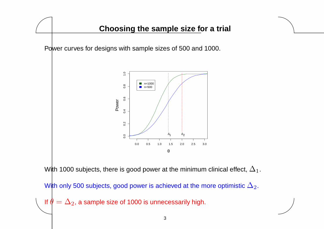
Power curves for designs with sample sizes of 500 and 1000.

0.0 0.5 1.0 1.5 2.0 2.5 3.0

0.0

0.2

0.4

0.6

0.8

1.0

θ

Pow

er

∆1 ∆2

n=1000n=500

With 1000 subjects, there is good power at the minimum clinical effect, ∆1.

With only 500 subjects, good power is achieved at the more optimistic ∆2.

If θ = ∆2, a sample size of 1000 is unnecessarily high.

3

'

&

$

%

Designing a trial with good power and sample size

In designing a clinical trial, we aim to

Protect the type I error rate,

Achieve sufficient power,

Use as small a sample size as possible.

Adaptive designs in this context often have the form:

Start with a fixed sample size design,

Examine interim data,

Add observations to improve power where most appropriate.

In contrast, Group Sequential designs require one to:

Specify the desired type I error and power function,

Set maximum sample size a little higher than the fixed sample size,

Stop the trial early if data support this.

4

'

&

$

%

Designing a clinical trial

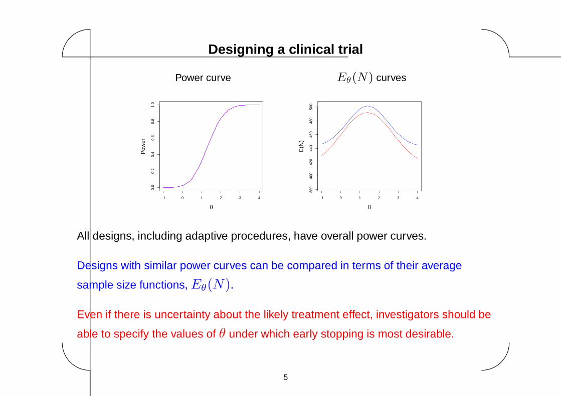
Power curve Eθ(N) curves

−1 0 1 2 3 4

0.0

0.2

0.4

0.6

0.8

1.0

θ

Pow

er

−1 0 1 2 3 4

380

400

420

440

460

480

500

θ

E(N

)

All designs, including adaptive procedures, have overall power curves.

Designs with similar power curves can be compared in terms of their average

sample size functions, Eθ(N).

Even if there is uncertainty about the likely treatment effect, investigators should be

able to specify the values of θ under which early stopping is most desirable.

5

'

&

$

%

Adaptive design or GST?

Jennison & Turnbull (JT) have compared group sequential tests (GSTs) and

adaptive designs. See, for example, papers in

Statistics in Medicine (2003, 2006), Biometrika (2006), Biometrics (2006)

JT conclude that:

GSTs are excellent

They do what is required with low expected sample sizes,

Error spending versions handle unpredictable group sizes, etc.

Adaptive designs can be as good as GSTs

However, many published adaptive designs require higher expected

sample sizes to achieve the same power as good GSTs.

6

'

&

$

%

Re-visiting the Group Sequential vs Adaptive question

The paper by Mehta & Pocock (Statistics in Medicine, 2011)

“Adaptive increase in sample size when interim results are promising:

A practical guide with examples”

has re-opened this question.

Conclusions of Mehta & Pocock (MP) are counter to the findings we have reported.

An important feature:

In MP’s first example, response is measured some time after treatment.

Thus, at an interim analysis, many patients have been treated but are yet to

produce a response.

Delayed responses are common — and not easily dealt with by standard GSTs.

7

'

&

$

%

Outline of talk

1. Mehta & Pocock’s Example 1

2. Mehta & Pocock’s design for this example

3. Alternative fixed and group sequential designs

4. Improving designs in Mehta & Pocock’s framework

5. Extending the framework

6. Relation to delayed response GSTs (Hampson & Jennison, JRSS B, 2013)

7. Conclusions

8

'

&

$

%

1. Mehta & Pocock’s Example

MP’s Example 1 concerns a Phase 3 trial of a new treatment for schizophrenia in

which a new drug is to be compared to an active comparator.

The efficacy endpoint is improvement in the Negative Symptoms Assessment score

from baseline to week 26.

Responses are

YBi ∼ N(µB, σ2), i = 1, 2, . . . , on the new treatment,

YAi ∼ N(µA, σ2), i = 1, 2, . . . , on the comparator treatment.

where σ2 = 7.52.

The treatment effect is

θ = µB − µA.

and we estimate θ by

θ = µB − µA = Y B − Y A.

9

'

&

$

%

Mehta & Pocock’s Example

The initial plan is for a total of n2 = 442 patients, 221 on each treatment.

In testing H0: θ ≤ 0 vs θ > 0, the final analysis will reject H0 if Z2

Z2 =θ(n2)√{4σ2/n2}

> 1.96.

This design and analysis gives type I error rate 0.025 and power 0.8 at θ = 2.

Higher power, e.g., power 0.8 at θ = 1.6, would be desirable.

But, the sponsors will only increase sample size if interim results are “promising”.

An interim analysis is planned after observing n1 = 208 responses.

10

'

&

$

%

Increasing the sample size

At the interim analysis with n1 = 208 observed responses, the estimated

treatment effect is

θ1(n1) = Y B(n1) − Y A(n1)

and

Z1 =θ1(n1)√{4σ2/n1}

.

At the time of this analysis, a further 208 subjects will have been treated for less

than 26 weeks. Their responses will be observed in due course.

As recruitment continues, we use the value of Z1 in choosing a new total sample

size between the original figure of 442 and a maximum of 884.

In deciding whether to increase the sample size, MP consider conditional power of

the original test (with n2 = 442 observations), given the observed value of Z1.

11

'

&

$

%

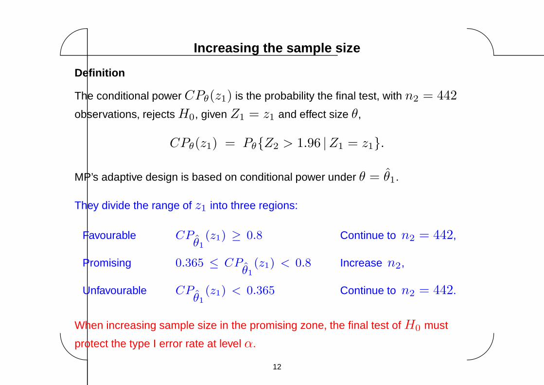
Increasing the sample size

Definition

The conditional power CPθ(z1) is the probability the final test, with n2 = 442

observations, rejects H0, given Z1 = z1 and effect size θ,

CPθ(z1) = Pθ{Z2 > 1.96 |Z1 = z1}.

MP’s adaptive design is based on conditional power under θ = θ1.

They divide the range of z1 into three regions:

Favourable CPθ1

(z1) ≥ 0.8 Continue to n2 = 442,

Promising 0.365 ≤ CPθ1

(z1) < 0.8 Increase n2,

Unfavourable CPθ1

(z1) < 0.365 Continue to n2 = 442.

When increasing sample size in the promising zone, the final test of H0 must

protect the type I error rate at level α.

12

'

&

$

%

The Chen, DeMets & Lan method

References:

Chen, DeMets & Lan, Statistics in Medicine (2004),

Gao, Ware & Mehta, J. Biopharmaceutical Statistics (2008).

Suppose at interim analysis 1, the final sample size is increased to n∗

2> n2 and a

final test is carried out without adjustment for this adaptation.

Thus, H0 is rejected if

Z2(n∗

2) =

θ(n∗

2)√{4σ2/n∗

2} > 1.96.

Chen, DeMets & Lan (CDL) show that if n2 is only increased when

CPθ1

(z1) > 0.5,

then the type I error probability will not increase.

(In general, changes to sample size may increase or decrease the type I error rate.)

13

'

&

$

%

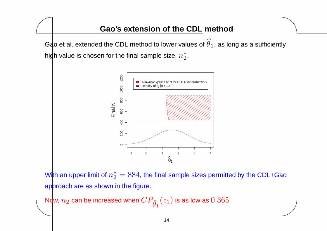
Gao’s extension of the CDL method

Gao et al. extended the CDL method to lower values of θ1, as long as a sufficiently

high value is chosen for the final sample size, n∗

2.

−1 0 1 2 3 4

020

040

060

080

010

0012

00

θ1

Fin

al N

Allowable values of N for CDL+Gao framework Density of θ1 (θ = 1.6)

With an upper limit of n∗

2= 884, the final sample sizes permitted by the CDL+Gao

approach are as shown in the figure.

Now, n2 can be increased when CPθ1

(z1) is as low as 0.365.

14

'

&

$

%

2. The MP design

In their “promising zone”, MP increase n2 to achieve conditional power 0.8 under

θ = θ1, truncating this value to 884 if it is larger than that.

−1 0 1 2 3 4

020

040

060

080

010

0012

00

θ1

Fin

al N

M−P adaptive design Density of θ1(θ = 1.6)

Comparison with the distribution of θ1 under θ = 1.6 shows that increases in n2

occur in a region of quite small probability.

The distribution of θ1 under other values of θ is shifted but has the same variance.

15

'

&

$

%

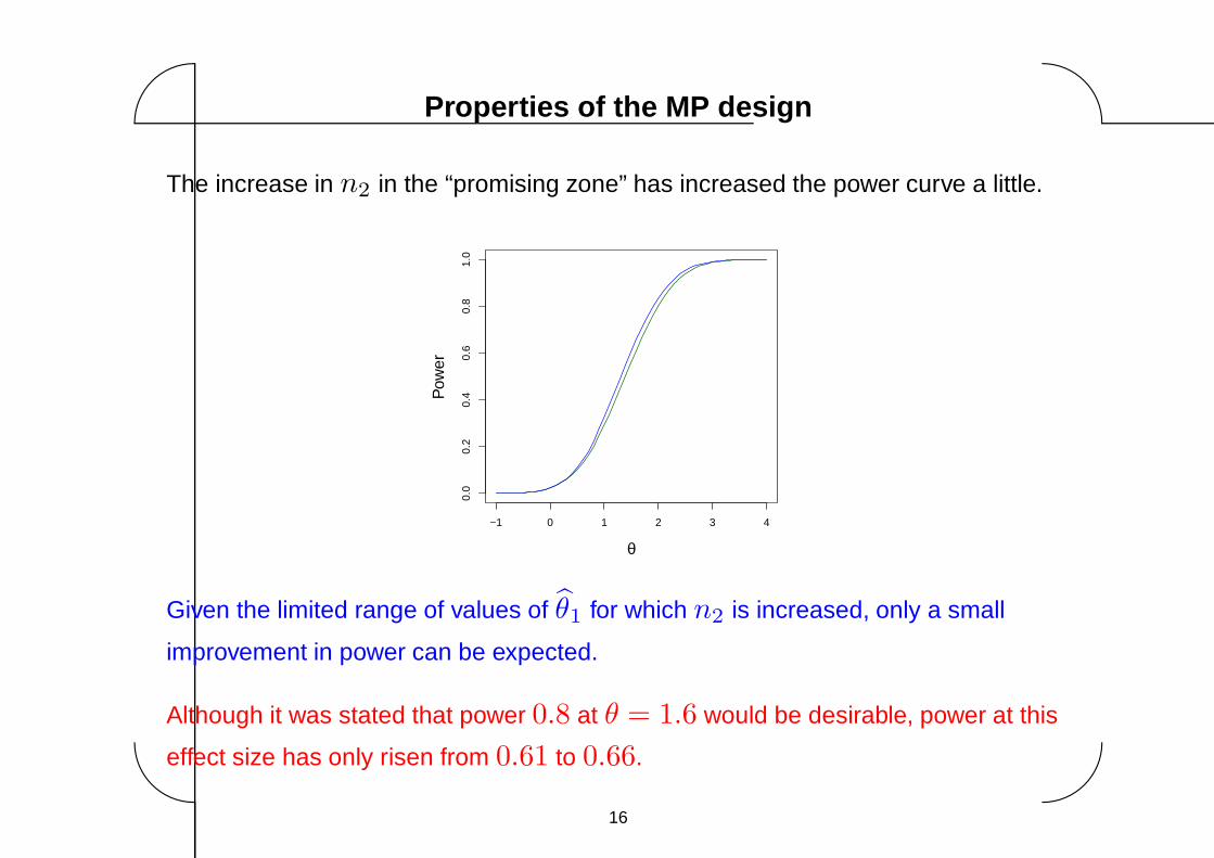
Properties of the MP design

The increase in n2 in the “promising zone” has increased the power curve a little.

−1 0 1 2 3 4

0.0

0.2

0.4

0.6

0.8

1.0

θ

Pow

er

Given the limited range of values of θ1 for which n2 is increased, only a small

improvement in power can be expected.

Although it was stated that power 0.8 at θ = 1.6 would be desirable, power at this

effect size has only risen from 0.61 to 0.66.

16

'

&

$

%

Properties of the MP design

The cost of higher power is an increase in expected sample size.

−1 0 1 2 3 4

380

400

420

440

460

480

500

θ

E(N

)

Aiming for higher conditional power under θ = θ1 or raising the sample size

beyond 884 gives small increases in power at the cost of large increases in E(N).

17

'

&

$

%

3. Alternatives to the MP design

Suppose we are satisfied with the overall power function attained by MP’s design.

The same power curve can be achieved by other designs.

A fixed sample design

Emerson, Levin & Emerson (Statistics in Medicine, 2011) note that the same power

is achieved by a fixed sample size study with 490 subjects.

This looks like an attractive option since, for effect sizes θ between 0.8 and 2.0, the

expected sample size of the MP design is greater than 490.

There is more to the sample size distribution than Eθ(N)

High variance in N is usually regarded as undesirable, so the wide variation in N

for the MP design is a negative feature.

Perhaps this might be viewed differently when a large increase in N represents an

influx of investment to a small bio-tech company?

18

'

&

$

%

A group sequential test

Despite the delayed response, we can still consider a group sequential design.

Suppose an interim analysis takes place after 208 observed responses.

If the trial stops at this analysis, the sample size is taken as 416, counting all

subjects treated thus far, even though only 208 have provided a response.

We consider an error spending design in the ρ-family (JT 2000, Ch. 7):

At analysis 1 after 208 responses

If Z1 ≥ 2.54 Stop, reject H0

If Z1 ≤ 0.12 Stop, accept H0

If 0.12 < Z1 < 2.54 Continue

At analysis 2 after 514 responses

If Z2 ≥ 2.00 Reject H0

If Z2 < 2.00 Accept H0

19

'

&

$

%

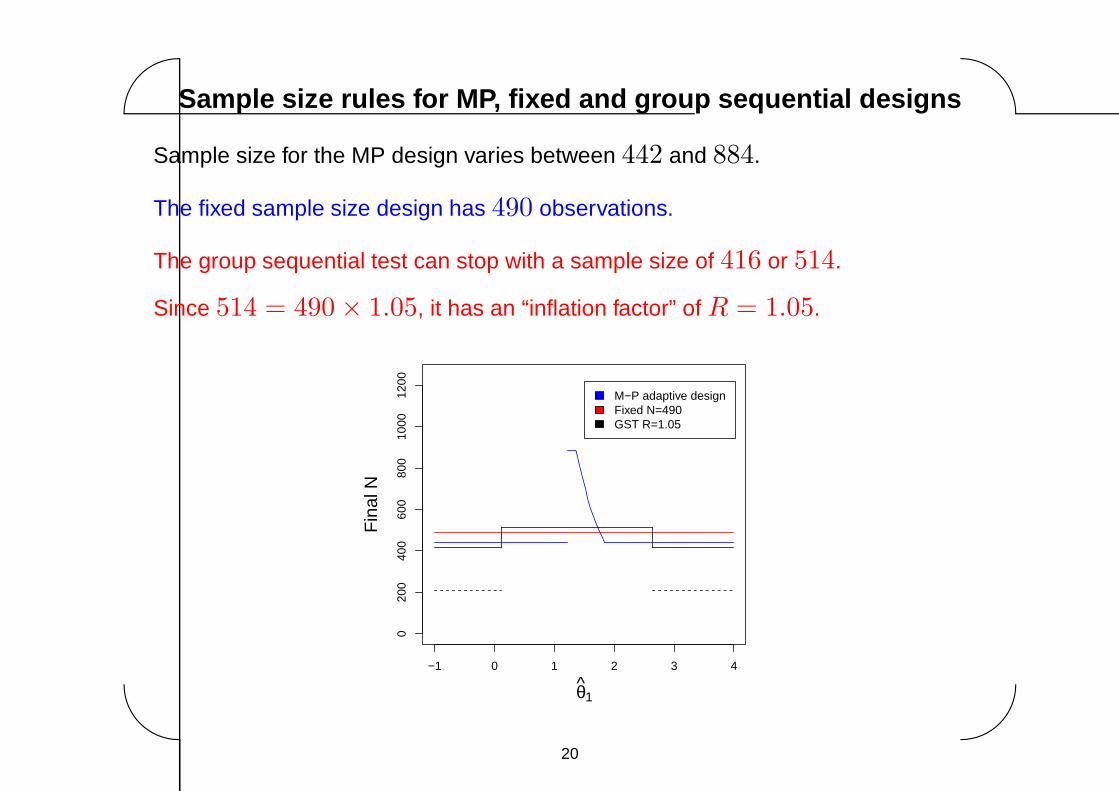
Sample size rules for MP, fixed and group sequential designs

Sample size for the MP design varies between 442 and 884.

The fixed sample size design has 490 observations.

The group sequential test can stop with a sample size of 416 or 514.

Since 514 = 490 × 1.05, it has an “inflation factor” of R = 1.05.

−1 0 1 2 3 4

020

040

060

080

010

0012

00

θ1

Fin

al N

M−P adaptive design Fixed N=490 GST R=1.05

20

'

&

$

%

Comparison of designs

Power curves Eθ(N) curves

−1 0 1 2 3 4

0.0

0.2

0.4

0.6

0.8

1.0

θ

Pow

er

M−P adaptive design Fixed N=490 GST R=1.05

−1 0 1 2 3 4

380

400

420

440

460

480

500

θ

E(N

)

M−P adaptive design Fixed N=490 GST R=1.05

All three designs have essentially the same power curve.

Clearly, it is quite possible to improve on the Eθ(N) curve of the MP design.

NB, Mehta & Pocock discuss two-stage group sequential designs but they only

present an example with much higher power (and, thus, higher sample size).

21

'

&

$

%

Can we improve the trial design within the MP framework?

Why does the MP design have high Eθ(N) for its achieved power?

Mehta & Pocock describe their method as adding observations in situations where

they will do the most good:

This seems a good idea, but the results are not so great,

Can we work out how to do this effectively?

22

'

&

$

%

4. Deriving efficient sample size rules in the MP framework

We stay with MP’s example and retain the basic elements of their design.

The interim analysis takes place after 208 observed responses.

A final sample size n∗

2is chosen based on θ1 (or equivalently Z1).

−1 0 1 2 3 4

020

040

060

080

010

0012

00

θ1

Fin

al N

Allowable values of N for CDL+Gao framework Values of n∗

2∈ [442, 884] that

satisfy the CDL+Gao conditions

are allowed.

At the final analysis, we reject

H0 if Z2 > 1.96, where Z2

is calculated without adjustment

for adaptation.

23

'

&

$

%

Efficient sample size rules in the MP framework

We shall assess the conditional power that an increase in sample size achieves.

Suppose Z1 = z1 and we are considering a final sample size n∗

2with

Z2(n∗

2) =

θ(n2)√{4σ2/n2}.

and conditional power under θ = θ

CPθ(z1, n

∗

2) = P

θ{Z2(n

∗

2) > 1.96 |Z1 = z1}.

Setting γ as a “rate of exchange” between sample size and power, we shall:

Choose n∗

2to optimise a combined objective

CPθ(z1, n∗

2) − γ(n∗

2− 442).

We shall do this with θ = 1.6, a value where we wish to “buy” additional power.

24

'

&

$

%

An overall optimality property

The rule that maximises CPθ(z1, n

∗

2(z1)) − γn∗

2(z1) for every z1 also

maximises, unconditionally,

Pθ=θ

(Reject H0) − γEθ(N).

This can be seen by writing Pθ=θ

(Reject H0) − γEθ(N) as

∫{CP

θ(z1, n

∗

2(z1)) − γn∗

2(z1)} f

θ(z1) dz1,

where fθ(z1) denotes the density of Z1 under θ = θ, and noting that we have

minimised the integrand for each z1.

We shall set γ = 0.14/(4 σ2) to achieve the same power curve as the MP design.

So, the resulting procedure will have minimum possible Eθ=1.6(N) among all

designs following the CDL+Gao framework that achieve power 0.658 at θ = 1.6.

25

'

&

$

%

Plots for θ = 1.6, γ = 0.14/(4 σ2) and θ1 = 1.5

500 600 700 800 900

0.5

0.6

0.7

0.8

0.9

1.0

Final N

Conditional powerCombined objective

The objective CPθ(z1, n

∗

2) − γ(n∗

2− 442) has a maximum at n∗

2= 654.

This value is similar to MP’s choice of n∗

2when θ1 = 1.5.

26

'

&

$

%

Plots for θ = 1.6, γ = 0.14/(4 σ2) and θ1 = 1.3

500 600 700 800 900

0.5

0.6

0.7

0.8

0.9

1.0

Final N

Conditional powerCombined objective

The conditional power curve is steeper and the optimum occurs at a higher n∗

2.

The objective CPθ(z1, n

∗

2) − γ(n∗

2− 442) is maximised at n∗

2= 707.

In this case, MP’s design takes the maximum permitted value of n∗

2= 884.

27

'

&

$

%

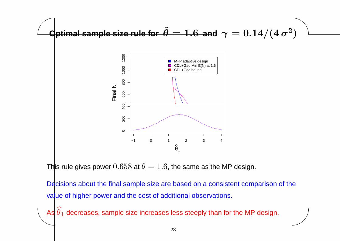
Optimal sample size rule for θ = 1.6 and γ = 0.14/(4 σ2)

−1 0 1 2 3 4

020

040

060

080

010

0012

00

θ1

Fin

al N

M−P adaptive design CDL+Gao Min E(N) at 1.6 CDL+Gao bound

This rule gives power 0.658 at θ = 1.6, the same as the MP design.

Decisions about the final sample size are based on a consistent comparison of the

value of higher power and the cost of additional observations.

As θ1 decreases, sample size increases less steeply than for the MP design.

28

'

&

$

%

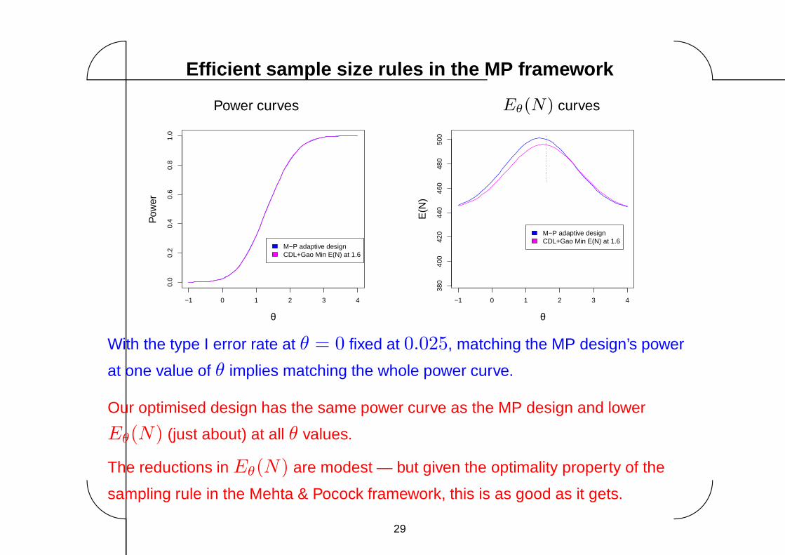
Efficient sample size rules in the MP framework

Power curves Eθ(N) curves

−1 0 1 2 3 4

0.0

0.2

0.4

0.6

0.8

1.0

θ

Pow

er

M−P adaptive design CDL+Gao Min E(N) at 1.6

−1 0 1 2 3 4

380

400

420

440

460

480

500

θ

E(N

)

M−P adaptive design CDL+Gao Min E(N) at 1.6

With the type I error rate at θ = 0 fixed at 0.025, matching the MP design’s power

at one value of θ implies matching the whole power curve.

Our optimised design has the same power curve as the MP design and lower

Eθ(N) (just about) at all θ values.

The reductions in Eθ(N) are modest — but given the optimality property of the

sampling rule in the Mehta & Pocock framework, this is as good as it gets.

29

'

&

$

%

Further efficiency gains

Our new, optimised procedure still has higher Eθ(N) than the two-stage GST that

ignores (but is charged for) pipeline data.

−1 0 1 2 3 4

380

400

420

440

460

480

500

θ

E(N

)

M−P adaptive design CDL+Gao Min E(N) at 1.6 GST R=1.05

−1 0 1 2 3 4

020

040

060

080

010

0012

00

θ1

Fin

al N

M−P adaptive design CDL+Gao Min E(N) at 1.6 CDL+Gao bound

Shapes of optimised sample size rules suggest it would help to increase n∗

2at

lower values of θ1 — but this is not permitted in the CDL+Gao framework.

The Conditional Probability of Rejection principle, or equivalently using a Bauer

& Kohne (Biometrics, 1994) Combination Test does allow such adaptations.

30

'

&

$

%

5. Using the Conditional Probability of Rejection principl e

Reference: Proschan & Hunsberger, (Biometrics, 1995)

On observing θ1, choose a new final sample size n∗

2.

Then, set the critical value for Z2(n∗

2) at the final analysis to maintain the

Conditional Probability of Rejection (CPR) under θ = 0 in the original design.

The overall type I error rate is the integral of the conditional type I error rate, and

this remains the same.

This type of adaptation can also be regarded as a “weighted inverse normal

combination test” Bauer & Kohne (1994).

We can follow our previous strategy in this new framework and set n∗

2to maximise

CPθ(z1, n

∗

2) − γ(n∗

2− 442). Again, we shall use θ = 1.6.

The resulting design has the minimum value of Eθ(N) among all designs in this

larger class that achieve the same power under θ = θ.

31

'

&

$

%

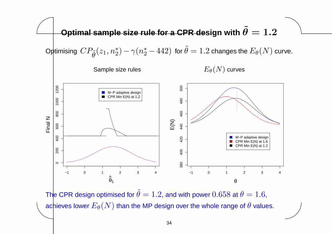
Optimal sample size rule for a CPR design with θ = 1.6

−1 0 1 2 3 4

020

040

060

080

010

0012

00

θ1

Fin

al N

M−P adaptive design CPR Min E(N) at 1.6

The rule with γ = 0.25/(4 σ2) matches the MP test’s power of 0.658 at θ = 1.6.

Shapes of optimised sample size rules are very different from the MP design.

The best opportunities for investing additional resource are not in Mehta & Pocock’s

“promising zone”.

32

'

&

$

%

Efficient sample size rules in the CPR framework

Eθ(N) curves

−1 0 1 2 3 4

380

400

420

440

460

480

500

θ

E(N

)

M−P adaptive design CDL+Gao Min E(N) at 1.6 CPR Min E(N) at 1.6

The CPR principle allows sample size increases for θ1 below the CDL+Gao region.

This leads to a useful reduction in Eθ(N) at θ = 1.6.

33

'

&

$

%

Optimal sample size rule for a CPR design with θ = 1.2

Optimising CPθ(z1, n

∗

2)− γ(n∗

2− 442) for θ = 1.2 changes the Eθ(N) curve.

Sample size rules Eθ(N) curves

−1 0 1 2 3 4

020

040

060

080

010

0012

00

θ1

Fin

al N

M−P adaptive design CPR Min E(N) at 1.2

−1 0 1 2 3 4

380

400

420

440

460

480

500

θ

E(N

)

M−P adaptive design CPR Min E(N) at 1.6 CPR Min E(N) at 1.2

The CPR design optimised for θ = 1.2, and with power 0.658 at θ = 1.6,

achieves lower Eθ(N) than the MP design over the whole range of θ values.

34

'

&

$

%

Further extensions

1. We can allow recruitment to be terminated at the interim analysis, so the

minimum final sample size is n2 = 416, rather than 442.

2. We can use a general conditional type I error function (Proschan & Hunsberger,

1995) or, equivalently, a general Bauer & Kohne (1994) combination rule.

3. We can minimise other sample size criteria, such as a weighted sum or integral

∑

i

wi Eθi(N) or

∫w(θ) Eθi

(N) dθ.

The resulting designs deal neatly with the “pipeline” subjects arising when there is a

delayed response.

They will give the best possible sampling and decision rules with n1 = 208 and

n2 in the range 416 to 884.

(We could also aim for higher power, now we have a good way to achieve this.)

35

'

&

$

%

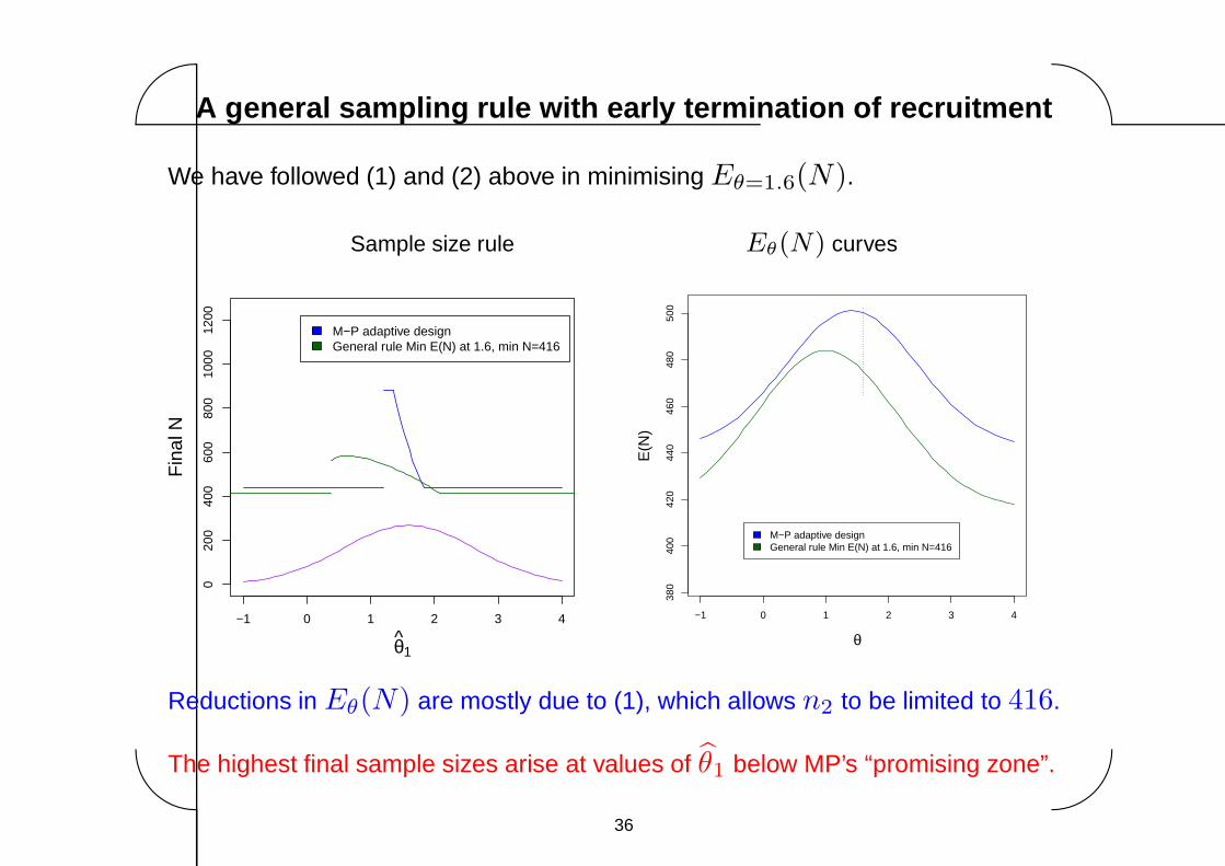
A general sampling rule with early termination of recruitme nt

We have followed (1) and (2) above in minimising Eθ=1.6(N).

Sample size rule Eθ(N) curves

−1 0 1 2 3 4

020

040

060

080

010

0012

00

θ1

Fin

al N

M−P adaptive design General rule Min E(N) at 1.6, min N=416

−1 0 1 2 3 4

380

400

420

440

460

480

500

θE

(N)

M−P adaptive design General rule Min E(N) at 1.6, min N=416

Reductions in Eθ(N) are mostly due to (1), which allows n2 to be limited to 416.

The highest final sample sizes arise at values of θ1 below MP’s “promising zone”.

36

'

&

$

%

6. Relation to proposals for Delayed Response GSTs

Reference: Hampson & Jennison, JRSS B (2013).

Hampson & Jennison have extended methodology for group sequential tests to

handle a delayed response.

Their “Delayed Response GSTs” allow any number of interim analyses and can be

optimised for specified criteria.

Applying this approach in the case of just 2 analyses:

Either recruitment stops at analysis 1 and the final analysis occurs when all

pipeline subjects have been observed,

Or, an additional group of subjects is recruited and the final analysis has

pipeline subjects plus these new subjects.

Thus, we have a special case of the designs we have been developing where only

two values of n2 are possible.

37

'

&

$

%

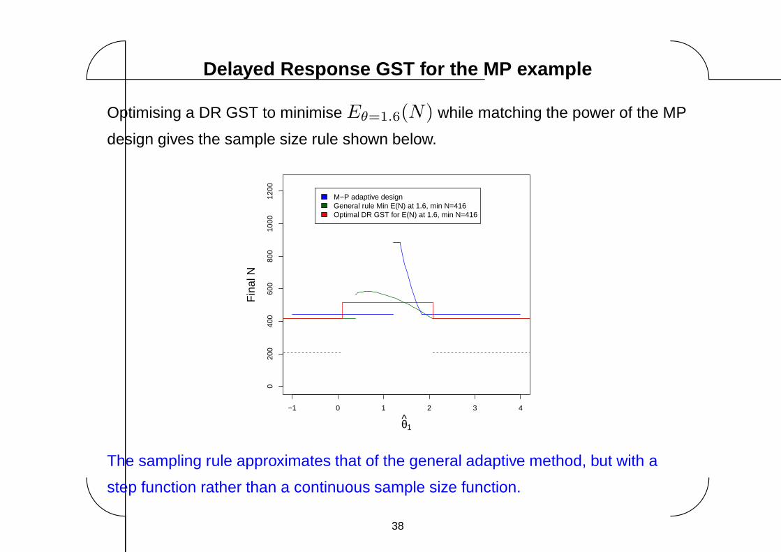
Delayed Response GST for the MP example

Optimising a DR GST to minimise Eθ=1.6(N) while matching the power of the MP

design gives the sample size rule shown below.

−1 0 1 2 3 4

020

040

060

080

010

0012

00

θ1

Fin

al N

M−P adaptive design General rule Min E(N) at 1.6, min N=416 Optimal DR GST for E(N) at 1.6, min N=416

The sampling rule approximates that of the general adaptive method, but with a

step function rather than a continuous sample size function.

38

'

&

$

%

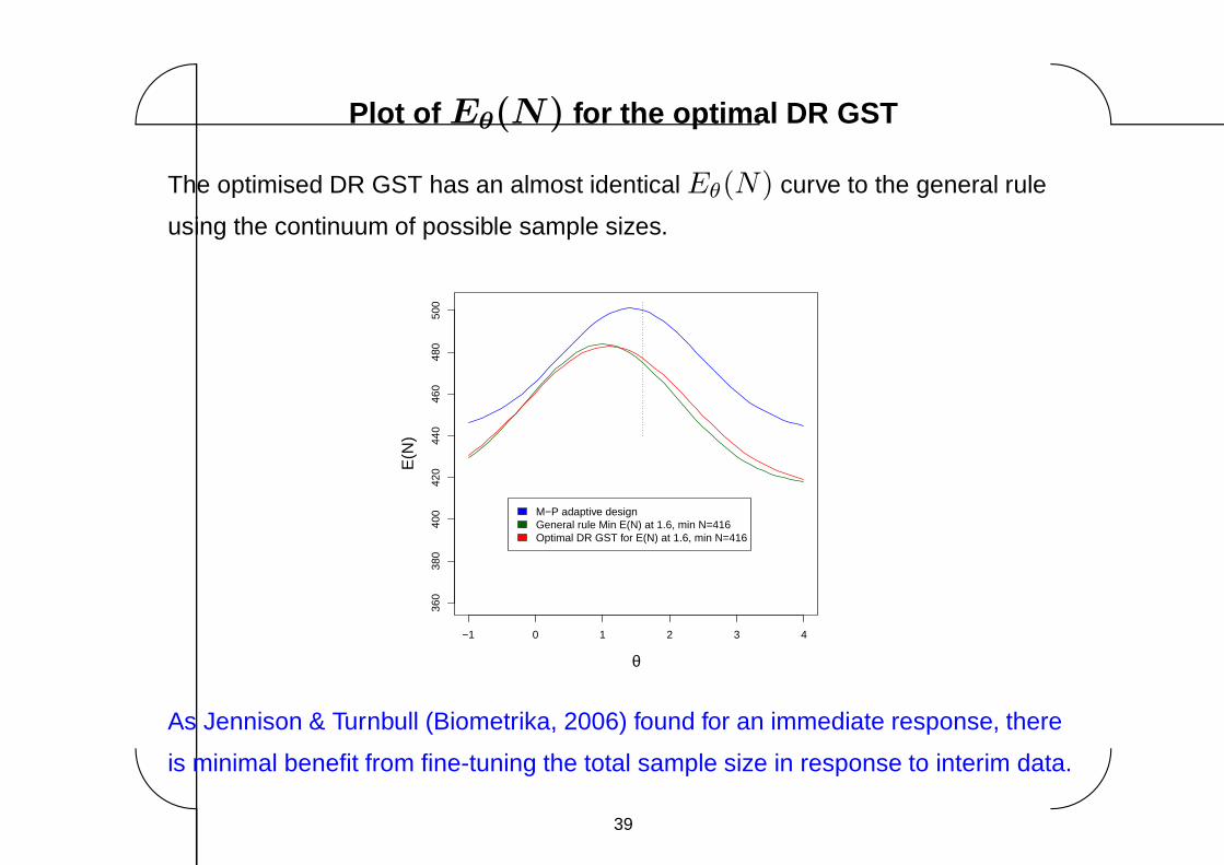
Plot of Eθ(N) for the optimal DR GST

The optimised DR GST has an almost identical Eθ(N) curve to the general rule

using the continuum of possible sample sizes.

−1 0 1 2 3 4

360

380

400

420

440

460

480

500

θ

E(N

)

M−P adaptive design General rule Min E(N) at 1.6, min N=416 Optimal DR GST for E(N) at 1.6, min N=416

As Jennison & Turnbull (Biometrika, 2006) found for an immediate response, there

is minimal benefit from fine-tuning the total sample size in response to interim data.

39

'

&

$

%

7. Conclusions

Although JT had previously shown that adaptive designs offer at most a slight

improvement on GSTs, it is appropriate to re-visit this issue for the case of a

delayed response, as in Mehta & Pocock’s example.

1. MP use the Chen, DeMets & Lan (2004) approach, choosing sample size

by a conditional power rule. This does not yield a particularly efficient design.

2. We have developed MP’s idea of spending resources where they have the

greatest benefit — and found efficient adaptive designs for this problem.

3. The solution to our most general version of the problem is very similar to a

“Delayed Response GST”, as proposed by Hampson & Jennison (2013).

Following this approach offers the benefits of established group sequential

methodology and its extensions, e.g., error spending tests.

4. If used well, the adaptive approach (start small, then ask for more) can

give good trial designs — but there are pitfalls to be avoided!

40