Chordal decomposition in operator-splitting methods...

Noname manuscript No.(will be inserted by the editor)

Chordal decomposition in operator-splitting methods forsparse semidefinite programs

Yang Zheng1 · Giovanni Fantuzzi2 ·Antonis Papachristodoulou1 · Paul Goulart1 ·Andrew Wynn2

Received: date / Accepted: date

Abstract We employ chordal decomposition to reformulate a large and sparse semidefiniteprogram (SDP), either in primal or dual standard form, into an equivalent SDP with smallerpositive semidefinite (PSD) constraints. In contrast to previous approaches, the decomposedSDP is suitable for the application of first-order operator-splitting methods, enabling thedevelopment of efficient and scalable algorithms. In particular, we apply the alternatingdirections method of multipliers (ADMM) to solve decomposed primal- and dual-standard-form SDPs. Each iteration of such ADMM algorithms requires a projection onto an affinesubspace, and a set of projections onto small PSD cones that can be computed in parallel.We also formulate the homogeneous self-dual embedding (HSDE) of a primal-dual pair ofdecomposed SDPs, and extend a recent ADMM-based algorithm to exploit the structure ofour HSDE. The resulting HSDE algorithm has the same leading-order computational costas those for the primal or dual problems only, with the advantage of being able to identifyinfeasible problems and produce an infeasibility certificate. All algorithms are implementedin the open-source MATLAB solver CDCS. Numerical experiments on a range of large-scale SDPs demonstrate the computational advantages of the proposed methods comparedto common state-of-the-art solvers.

Keywords sparse SDPs · chordal decomposition · operator-splitting · first-order methods

YZ and GF contributed equally. A preliminary version of part of this work appeared in [47, 48]. YZ is sup-ported by Clarendon Scholarship and Jason Hu Scholarship. GF was supported in part by the EPSRC grantEP/J010537/1. AP was supported in part by EPSRC Grant EP/J010537/1 and EP/M002454/1.

Y. Zheng (�)Tel.: +44-07511784230E-mail: [email protected]. FantuzziE-mail: [email protected]. PapachristodoulouE-mail: [email protected]. GoulartE-mail: [email protected]. WynnE-mail: [email protected] Department of Engineering Science, University of Oxford, Parks Road, Oxford, OX1 3PJ, U.K.2 Department of Aeronautics, Imperial College London, South Kensington Campus, SW7 2AZ, U.K.

2 Y. Zheng, G. Fantuzzi, A. Papachristodoulou, P. Goulart and A. Wynn

Mathematics Subject Classification (2000) 90C06 · 90C22 · 90C25 · 49M27 · 49M29

1 Introduction

Semidefinite programs (SDPs) are convex optimization problems over the cone of positivesemidefinite (PSD) matrices. Given b ∈ Rm, C ∈ Sn, and matrices A1, . . . , Am ∈ Sn,the standard primal form of an SDP is

minX

〈C,X〉

s.t. 〈Ai, X〉 = bi, i = 1, . . . ,m,

X ∈ Sn+,

(1)

while the standard dual form is

maxy, Z

〈b, y〉

s.t. Z +m∑i=1

Ai yi = C,

Z ∈ Sn+.

(2)

In the above and throughout this work, Rm is the usual m-dimensional Euclidean space,Sn is the space of n × n symmetric matrices, Sn+ is the cone of PSD matrices, and 〈·, ·〉denotes the inner product in the appropriate space, i.e., 〈x, y〉 = xT y for x, y ∈ Rm and〈X,Y 〉 = trace(XY ) for X,Y ∈ Sn. SDPs have found applications in a wide range offields, such as control theory, machine learning, combinatorics, and operations research [8].Semidefinite programming encompasses other common types of optimization problems, in-cluding linear, quadratic, and second-order cone programs [10]. Furthermore, many nonlin-ear convex constraints admit SDP relaxations that work well in practice [39].

It is well-known that small and medium-sized SDPs can be solved up to any arbitraryprecision in polynomial time [39] using efficient second-order interior-point methods (IPM-s) [2,22]. However, many problems of practical interest are too large to be addressed by thecurrent state-of-the-art interior-point algorithms, largely due to the need to compute, store,and factorize an m×m matrix at each iteration.

A common strategy to address this shortcoming is to abandon IPMs in favour of sim-pler first-order methods (FOMs), at the expense of reducing the accuracy of the solution. Forinstance, Malick et al. introduced regularization methods to solve SDPs based on a dual aug-mented Lagrangian [28]. Wen et al. proposed an alternating direction augmented Lagrangianmethod for large-scale SDPs in the dual standard form [40]. Zhao et al. presented an aug-mented Lagrangian dual approach combined with the conjugate gradient method to solvelarge-scale SDPs [45]. More recently, O’Donoghue et al. developed a first-order operator-splitting method to solve the homogeneous self-dual embedding (HSDE) of a primal-dualpair of conic programs [29]. The algorithm, implemented in the C package SCS [30], hasthe advantage of providing certificates of primal or dual infeasibility.

A second major approach to resolve the aforementioned scalability issues is based on theobservation that the large-scale SDPs encountered in applications are often structured and/orsparse [8]. Exploiting sparsity in SDPs is an active and challenging area of research [3],with one main difficulty being that the optimal (primal) solution is typically dense evenwhen the problem data are sparse. Nonetheless, if the aggregate sparsity pattern of the

Chordal decomposition in operator-splitting methods for sparse SDPs 3

data is chordal (or has sparse chordal extensions), Grone’s [21] and Agler’s theorems [1]allow one to replace the original, large PSD constraint with a set of PSD constraints onsmaller matrices, coupled by additional equality constraints. Having reduced the size ofthe semidefinite variables, the converted SDP can in some cases be solved more efficientlythan the original problem using standard IPMs. These ideas underly the domain-space andthe range-space conversion techniques in [16, 24], implemented in the MATLAB packageSparseCoLO [15].

The problem with such decomposition techniques, however, is that the addition of e-quality constraints to an SDP often offsets the benefit of working with smaller semidefinitecones. One possible solution is to exploit the properties of chordal sparsity patterns directlyin the IPMs: Fukuda et al. used Grone’s positive definite completion theorem [21] to devel-op a primal-dual path-following method [16]; Burer proposed a nonsymmetric primal-dualIPM using Cholesky factors of the dual variable Z and maximum determinant completionof the primal variable X [11]; and Andersen et al. developed fast recursive algorithms toevaluate the function values and derivatives of the barrier functions for SDPs with chordalsparsity [4]. Another attractive option is to solve the sparse SDP using FOMs: Sun et al. pro-posed a first-order splitting algorithm for partially decomposable conic programs, includingSDPs with chordal sparsity [35]; Kalbat & Lavaei applied a first-order operator-splittingmethod to solve a special class of SDPs with fully decomposable constraints [23]; Madaniet al. developed a highly-parallelizable first-order algorithm for sparse SDPs with inequalityconstraints, with applications to optimal power flow problems [27].

In this work, we embrace the spirit of [23,27,29,35] and exploit sparsity in SDPs using afirst-order operator-splitting method known as the alternating direction method of multipli-ers (ADMM). Introduced in the mid-1970s [17, 19], ADMM is related to other FOMs suchas dual decomposition and the method of multipliers, and it has recently found applicationsin many areas, including covariance selection, signal processing, resource allocation, andclassification; see [9] for a review. More precisely, our contributions are:

1. Using Grone’s theorem [21] and Agler’s theorem [1], we formulate domain-space andrange-space conversion frameworks for primal- and dual-standard-form sparse SDPswith chordal sparsity, respectively. These resemble the conversion methods developedin [16, 24] for IPMs, but are more suitable for the application of FOMs. One majordifference with [16,24] is that we introduce two sets of slack variables, so that the conicand the affine constraints can be separated when using operator-splitting algorithms.

2. We apply ADMM to solve the domain- and range-space converted SDPs, and show thatthe resulting iterates of the ADMM algorithms are the same up to scaling. The iterationsare cheap: the positive semidefinite (PSD) constraint is enforced via parallel projectionsonto small PSD cones — a computationally cheaper strategy than that in [35], whileimposing the affine constraints requires solving a linear system with constant coefficientmatrix, the factorization/inverse of which can be cached before iterating the algorithm.

3. We formulate the HSDE of a converted primal-dual pair of sparse SDPs. In contrastto [23, 27, 35], this allows us to compute either primal and dual optimal points, or acertificate of infeasibility. In particular, we extend the algorithm proposed in [29] toexploit the structure of our HSDE, reducing its computational complexity. The resultingalgorithm is more efficient than a direct application of the method of [29] to eitherthe original primal-dual pair (i.e. before chordal sparsity is taken into account), or theconverted problems: in the former case, the chordal decomposition reduces the costof the conic projections; in the latter case, we speed up the projection onto the affineconstraints using a series of block-eliminations.


1 4

2 3

(a)

1 4

2 3

(b)

Fig. 1 (a) Nonchordal graph: the cycle (1-2-3-4) has length four but no chords. (b) Chordal graph: all cyclesof length no less than four have a chord; the maximal cliques are C1 = {1, 2, 4} and C2 = {2, 3, 4}.

4. We present the MATLAB solver CDCS (Cone Decomposition Conic Solver), whichimplements our ADMM algorithms. CDCS is the first open-source first-order solverthat exploits chordal decomposition and can detect infeasible problems. We test ourimplementation on large-scale sparse problems in SDPLIB [7], selected sparse SDPswith nonchordal sparsity pattern [4], and randomly generated SDPs with block-arrowsparsity patterns [35]. The results demonstrate the efficiency of our algorithms comparedto the interior-point solvers SeDuMi [34] and the first-order solver SCS [30].

The rest of the paper is organized as follows. Section 2 reviews chordal decomposi-tion and the basic ADMM algorithm. Section 3 introduces our conversion framework forsparse SDPs based on chordal decomposition. We show how to apply the ADMM to exploitdomain-space and range-space sparsity in primal and dual SDPs in Section 4. Section 5 dis-cusses the ADMM algorithm for the HSDE of SDPs with chordal sparsity. CDCS and ournumerical experiments are presented in Section 6. Section 7 concludes the paper.

2 Preliminaries

2.1 A review of graph theoretic notions

We start by briefly reviewing some key graph theoretic concepts (see [6,20] for more details).A graph G(V, E) is defined by a set of vertices V = {1, 2, . . . , n} and a set of edgesE ⊆ V × V . A graph G(V, E) is called complete if any two nodes are connected by anedge. A subset of vertices C ⊆ V such that (i, j) ∈ E for any distinct vertices i, j ∈ C,i.e., such that the subgraph induced by C is complete, is called a clique. The number ofvertices in C is denoted by |C|. If C is not a subset of any other clique, then it is referredto as a maximal clique. A cycle of length k in a graph G is a set of pairwise distinct nodes{v1, v2, . . . , vk} ⊂ V such that (vk, v1) ∈ E and (vi, vi+1) ∈ E for i = 1, . . . , k − 1. Achord is an edge joining two non-adjacent nodes in a cycle.

An undirected graph G is called chordal (or triangulated, or a rigid circuit [38]) if everycycle of length greater than or equal to four has at least one chord. Chordal graphs includeseveral other classes of graphs, such as acyclic undirected graphs (including trees) and com-plete graphs. Algorithms such as the maximum cardinality search [36] can test chordalityand identify the maximal cliques of a chordal graph efficiently, i.e., in linear time in termsof the number of nodes and edges. Non-chordal graphs can always be chordal extended,i.e., extended to a chordal graph, by adding additional edges to the original graph. Comput-ing the chordal extension with the minimum number of additional edges is an NP-completeproblem [42], but several heuristics exist to find a good chordal extensions efficiently [38].

Fig. 1 illustrates these concepts. The graph in Fig. 1(a) is not chordal, but can be chordalextended to the graph in Fig. 1(b) by adding the edge (2, 4). The chordal graph in Fig. 1(b)


(a) (b) (c)

Fig. 2 Examples of chordal graphs: (a) banded graph; (b) block-arrow; (c) a generic chordal graph.

(a) (b) (c)

Fig. 3 Sparsity patterns of 8× 8 matrices corresponding to the 8-node graphs in Fig. 2(a)–(c).

has two maximal cliques, C1 = {1, 2, 4} and C2 = {2, 3, 4}. Other examples of chordalgraphs are given in Fig. 2.

2.2 Sparse matrix cones and chordal decomposition

The sparsity pattern of a symmetric matrix X ∈ Sn can be represented by an undirectedgraph G(V, E), and vice-versa. For example, the graphs in Fig. 2 correspond to the sparsitypatterns illustrated in Fig. 3. With a slight abuse of terminology, we refer to the graph G asthe sparsity pattern of X . Given a clique Ck of G, we define a matrix ECk ∈ R|Ck|×n as

(ECk)ij =

{1, if Ck(i) = j

0, otherwise

where Ck(i) is the i-th vertex in Ck, sorted in the natural ordering. Given X ∈ Sn, thematrix ECk can be used to select a principal submatrix defined by the clique Ck, i.e.,ECkXE

TCk ∈ S|Ck|. In addition, the operationETCkY ECk creates an n×n symmetric matrix

from a |Ck| × |Ck| matrix. For example, the chordal graph in Fig. 1(b) has a maximal cliqueC1 = {1, 2, 4}, and for Y ∈ S3 we have

EC1 =

1 0 0 00 1 0 00 0 0 1

, EC1XETC1 =

X11 X12 X14

X21 X22 X24

X41 X42 X44

, ETC1Y EC1 =

Y11 Y12 0 Y13Y21 Y22 0 Y230 0 0 0Y31 Y32 0 Y33

.Given an undirected graph G(V, E), let E∗ = E ∪{(i, i),∀ i ∈ V} be a set of edges that

includes all self-loops. We define the space of sparse symmetric matrices represented by Gas

Sn(E , 0) := {X ∈ Sn|Xij = Xji = 0 if (i, j) /∈ E∗},


and the cone of sparse PSD matrices as

Sn+(E , 0) := {X ∈ Sn(E , 0) : X � 0}.

Moreover, we consider the cone

Sn+(E , ?) := PSn(E,0)(Sn+)

given by the projection of the PSD cone onto the space of sparse matrices Sn(E , 0) withrespect to the usual Frobenius matrix norm (this is the norm induced by the usual trace innerproduct on the space of symmetric matrices). In is not difficult to see that X ∈ Sn+(E , ?) ifand only if it has a positive semidefinite completion, i.e., if there exists M � 0 such thatMij = Xij when (i, j) ∈ E∗.

For any undirected graph G(V, E), the cones Sn+(E , ?) and Sn+(E , 0) are dual to eachother with respect to the trace inner product in the space of sparse matrices Sn(E , 0) [38].In other words,

Sn+(E , ?) ≡ {X ∈ Sn(E , 0) : 〈X,Z〉 ≥ 0, ∀Z ∈ Sn+(E , 0)},Sn+(E , 0) ≡ {Z ∈ Sn(E , 0) : 〈Z,X〉 ≥ 0, ∀X ∈ Sn+(E , ?)}.

If G is chordal, then Sn+(E , ?) and Sn+(E , 0) can be equivalently decomposed into a setof smaller but coupled convex cones according to the following theorems:

Theorem 1 (Grone’s theorem [21]) Let G(V, E) be a chordal graph, and let {C1, C2, . . . , Cp}be the set of its maximal cliques. Then, X ∈ Sn+(E , ?) if and only if

ECkXETCk ∈ S|Ck|+ , k = 1, . . . , p.

Theorem 2 (Agler’s theorem [1]) Let G(V, E) be a chordal graph, and let {C1, C2, . . . , Cp}be the set of its maximal cliques. Then, Z ∈ Sn+(E , 0) if and only if there exist matricesZk ∈ S|Ck|+ for k = 1, . . . , p such that

Z =

p∑k=1

ETCkZkECk .

Note that these results can be proven individually, but can also be derived from each otherusing the duality of the cones Sn+(E , ?) and Sn+(E , 0) [24]. In this paper, the terminologychordal (or clique) decomposition of a sparse matrix cone will refer to the application ofTheorem 1 or Theorem 2 to replace a large sparse PSD cone with a set of smaller butcoupled PSD cones. Chordal decomposition of sparse matrix cones underpins much of therecent research on sparse SDPs [4,16,24,27,35,38], most of which relies on the conversionframework for IPMs proposed in [16, 24].

To illustrate the concept, consider the chordal graph in Fig. 1(b). According to Grone’stheorem,X11 X12 0 X14

X12 X22 X23 X24

0 X23 X33 X34

X14 X24 X34 X44

∈ Sn+(E , ?) ⇔

X11 X12 X14

X12 X22 X24

X14 X24 X44

� 0,

X22 X23 X24

X23 X33 X34

X24 X34 X44

� 0.


Similarly, Agler’s theorem guarantees that (after eliminating some of the variables)

Z11 Z12 0 Z14

Z12 Z22 Z23 Z24

0 Z23 Z33 Z34

Z14 Z24 Z34 Z44

∈ Sn+(E , 0) ⇔

Z11 Z12 Z14

Z12 a2 a3

Z14 a3 a4

� 0,

b2 Z23 b3

Z23 Z33 Z34

b3 Z34 b4

� 0,

ai + bi = Zii, i ∈ {2, 4},a3 + b3 = Z24.

Note that the PSD contraints obtained after the chordal decomposition of X (resp. Z) arecoupled via the elements X22, X44, and X24 = X42 (resp. Z22, Z44, and Z24 = Z42).

2.3 The Alternating Direction Method of Multipliers

The computational “engine” employed in this work is the alternating direction method ofmultipliers (ADMM). ADMM is an operator-splitting method developed in the 1970s, andit is known to be equivalent to other operator-splitting methods such as Douglas-Rachfordsplitting and Spingarn’s method of partial inverses; see [9] for a review. The ADMM algo-rithm solves the optimization problem

minx,y

f(x) + g(y)

s.t. Ax+By = c,(3)

where f and g are convex functions, x ∈ Rnx , y ∈ Rny , A ∈ Rnc×nx , B ∈ Rnc×ny andc ∈ Rnc . Given a penalty parameter ρ > 0 and a dual multiplier z ∈ Rnc , the ADMMalgorithm finds a saddle point of the augmented Lagrangian

Lρ(x, y, z) := f(x) + g(y) + zT (Ax+By − c) +ρ

2‖Ax+By − c‖2

by minimizing L with respect to the primal variables x and y separately, followed by a dualvariable update:

x(n+1) = arg minxLρ(x, y(n), z(n)), (4a)

y(n+1) = arg minyLρ(x(n+1), y, z(n)), (4b)

z(n+1) = z(n) + ρ (Ax(n+1) +By(n+1) − c). (4c)

The superscript (n) indicates that a variable is fixed to its value at the n-th iteration. Notethat since z is fixed in (4a) and (4b), one may equivalently minimize the modified Lagrangian

Lρ(x, y, z) := f(x) + g(y) +ρ

2

∥∥∥∥Ax+By − c+1

ρz

∥∥∥∥2 .Under very mild conditions, the ADMM converges to a solution of (3) with a rateO( 1

n )[9, Section 3.2]. ADMM is particularly suitable when (4a) and (4b) have closed-form ex-pressions, or can be solved efficiently. Moreover, splitting the minimization over x and yoften allows distributed and/or parallel implementations of steps (4a)–(4c).


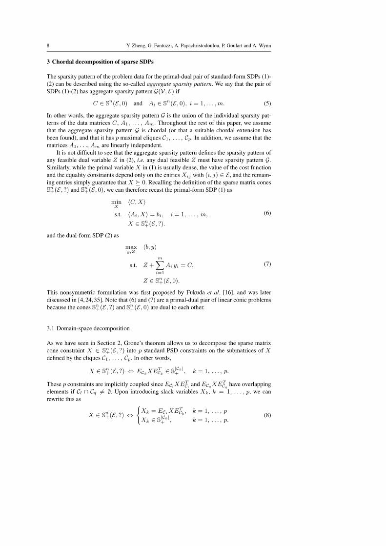
3 Chordal decomposition of sparse SDPs

The sparsity pattern of the problem data for the primal-dual pair of standard-form SDPs (1)-(2) can be described using the so-called aggregate sparsity pattern. We say that the pair ofSDPs (1)-(2) has aggregate sparsity pattern G(V, E) if

C ∈ Sn(E , 0) and Ai ∈ Sn(E , 0), i = 1, . . . ,m. (5)

In other words, the aggregate sparsity pattern G is the union of the individual sparsity pat-terns of the data matrices C, A1, . . . , Am. Throughout the rest of this paper, we assumethat the aggregate sparsity pattern G is chordal (or that a suitable chordal extension hasbeen found), and that it has p maximal cliques C1, . . . , Cp. In addition, we assume that thematrices A1, . . ., Am are linearly independent.

It is not difficult to see that the aggregate sparsity pattern defines the sparsity pattern ofany feasible dual variable Z in (2), i.e. any dual feasible Z must have sparsity pattern G.Similarly, while the primal variable X in (1) is usually dense, the value of the cost functionand the equality constraints depend only on the entries Xij with (i, j) ∈ E , and the remain-ing entries simply guarantee that X � 0. Recalling the definition of the sparse matrix conesSn+(E , ?) and Sn+(E , 0), we can therefore recast the primal-form SDP (1) as

minX

〈C,X〉

s.t. 〈Ai, X〉 = bi, i = 1, . . . , m,

X ∈ Sn+(E , ?).

(6)

and the dual-form SDP (2) as

maxy,Z

〈b, y〉

s.t. Z +m∑i=1

Ai yi = C,

Z ∈ Sn+(E , 0).

(7)

This nonsymmetric formulation was first proposed by Fukuda et al. [16], and was laterdiscussed in [4,24,35]. Note that (6) and (7) are a primal-dual pair of linear conic problemsbecause the cones Sn+(E , ?) and Sn+(E , 0) are dual to each other.

3.1 Domain-space decomposition

As we have seen in Section 2, Grone’s theorem allows us to decompose the sparse matrixcone constraint X ∈ Sn+(E , ?) into p standard PSD constraints on the submatrices of Xdefined by the cliques C1, . . . , Cp. In other words,

X ∈ Sn+(E , ?) ⇔ ECkXETCk ∈ S|Ck|+ , k = 1, . . . , p.

These p constraints are implicitly coupled since EClXETCl and ECqXE

TCq have overlapping

elements if Cl ∩ Cq 6= ∅. Upon introducing slack variables Xk, k = 1, . . . , p, we canrewrite this as

X ∈ Sn+(E , ?) ⇔

{Xk = ECkXE

TCk , k = 1, . . . , p

Xk ∈ S|Ck|+ , k = 1, . . . , p.(8)


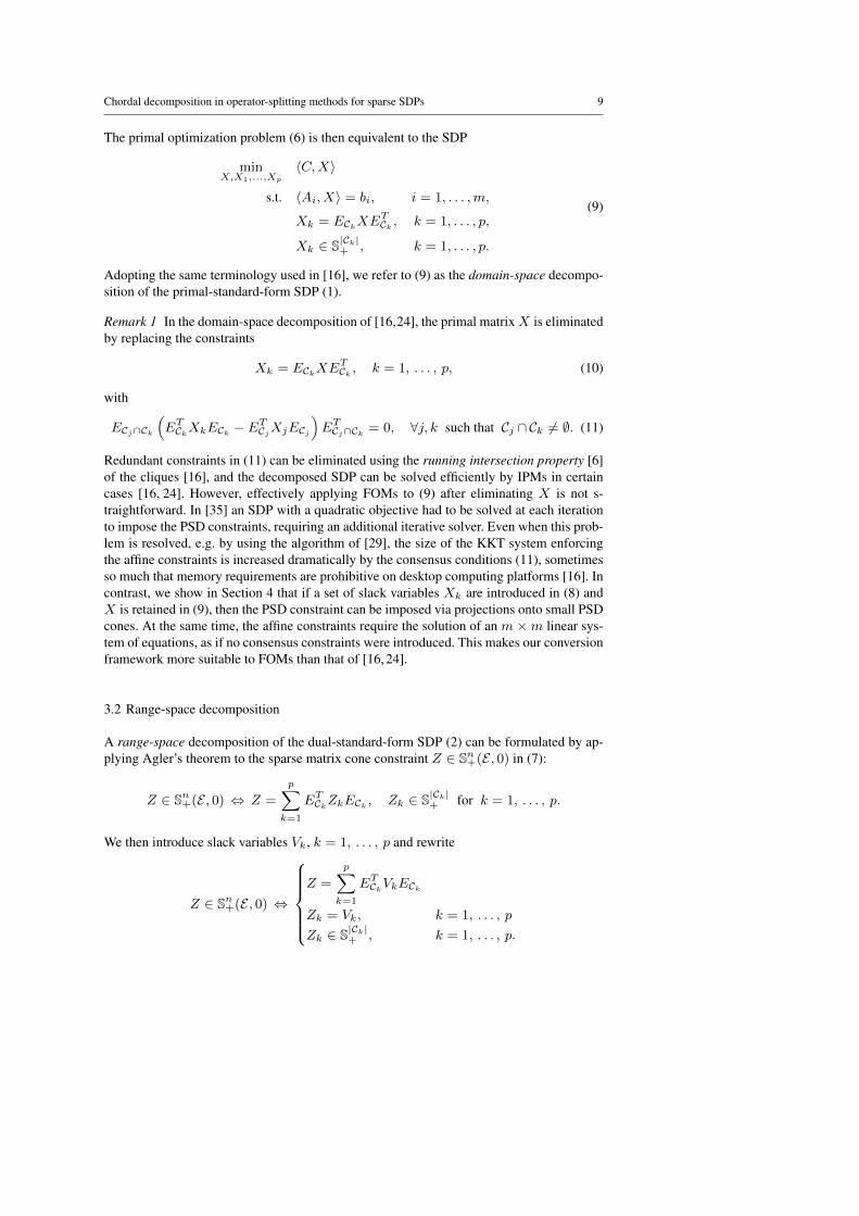
The primal optimization problem (6) is then equivalent to the SDP

minX,X1,...,Xp

〈C,X〉

s.t. 〈Ai, X〉 = bi, i = 1, . . . ,m,

Xk = ECkXETCk , k = 1, . . . , p,

Xk ∈ S|Ck|+ , k = 1, . . . , p.

(9)

Adopting the same terminology used in [16], we refer to (9) as the domain-space decompo-sition of the primal-standard-form SDP (1).

Remark 1 In the domain-space decomposition of [16,24], the primal matrixX is eliminatedby replacing the constraints

Xk = ECkXETCk , k = 1, . . . , p, (10)

with

ECj∩Ck

(ETCkXkECk − E

TCjXjECj

)ETCj∩Ck = 0, ∀j, k such that Cj ∩Ck 6= ∅. (11)

Redundant constraints in (11) can be eliminated using the running intersection property [6]of the cliques [16], and the decomposed SDP can be solved efficiently by IPMs in certaincases [16, 24]. However, effectively applying FOMs to (9) after eliminating X is not s-traightforward. In [35] an SDP with a quadratic objective had to be solved at each iterationto impose the PSD constraints, requiring an additional iterative solver. Even when this prob-lem is resolved, e.g. by using the algorithm of [29], the size of the KKT system enforcingthe affine constraints is increased dramatically by the consensus conditions (11), sometimesso much that memory requirements are prohibitive on desktop computing platforms [16]. Incontrast, we show in Section 4 that if a set of slack variables Xk are introduced in (8) andX is retained in (9), then the PSD constraint can be imposed via projections onto small PSDcones. At the same time, the affine constraints require the solution of an m×m linear sys-tem of equations, as if no consensus constraints were introduced. This makes our conversionframework more suitable to FOMs than that of [16, 24].

3.2 Range-space decomposition

A range-space decomposition of the dual-standard-form SDP (2) can be formulated by ap-plying Agler’s theorem to the sparse matrix cone constraint Z ∈ Sn+(E , 0) in (7):

Z ∈ Sn+(E , 0) ⇔ Z =

p∑k=1

ETCkZkECk , Zk ∈ S|Ck|+ for k = 1, . . . , p.

We then introduce slack variables Vk, k = 1, . . . , p and rewrite

Z ∈ Sn+(E , 0) ⇔

Z =

p∑k=1

ETCkVkECk

Zk = Vk, k = 1, . . . , p

Zk ∈ S|Ck|+ , k = 1, . . . , p.


Primal SDP (1) Dual SDP (2)

Decomposed Primal SDP (9) Decomposed Dual SDP (12)

Algorithm 1 Algorithm 2

Grone’s Theorem Agler’s Theorem

Duality

Duality

ADMM ADMMScaling

Fig. 4 Duality between the original primal and dual SDPs, and the decomposed primal and dual SDPs.

Similar comments as in Remark 1 hold, and the slack variables V1, . . . , Vp are essentialto formulate a decomposition framework suitable for the application of FOMs. The range-space decomposition of (2) is then given by

maxy,Z,V1,...,Vp

〈b, y〉

s.t.m∑i=1

Ai yi +

p∑k=1

ETCkVkECk = C,

Zk − Vk = 0, k = 1, . . . , p,

Zk ∈ S|Ck|+ , k = 1, . . . , p.

(12)

Remark 2 Although the domain- and range-space decompositions (9) and (12) have beenderived individually, they are in fact a primal-dual pair of SDPs. The duality between theoriginal SDPs (1) and (2) is inherited by the decomposed SDPs (9) and (12) by virtue of theduality between Grone’s and Agler’s theorems. This elegant picture is illustrated in Fig. 4.

4 ADMM for domain- and range-space decompositions of sparse SDPs

In this section, we demonstrate how ADMM can be applied to solve the domain-space de-composition (9) and the range-space decomposition (12) efficiently. Furthermore, we showthat the resulting domain- and range-space algorithms are equivalent, in the sense that oneis just a scaled version of the other. Throughout this section, δK(x) will denote the indicatorfunction of a set K, i.e.

δK(x) =

{0, if x ∈ K,+∞, otherwise.

For notational neatness, however, we write δ0 when K ≡ {0}.To ease the exposition further, we consider the usual vectorized forms of (9) and (12).

Specifically, we let vec : Sn → Rn2

be the usual operator mapping a matrix to the stack ofits column and define the vectorized data

c := vec(C), A :=[vec(A0) . . . vec(Am)

]T.

Note that the assumption that A1, . . ., Am are linearly independent matrices means that Ahas full row rank. For all k = 1, . . . , p, we also introduce the vectorized variables

x := vec(X), xk := vec(Xk), zk := vec(Zk), vk := vec(Vk),


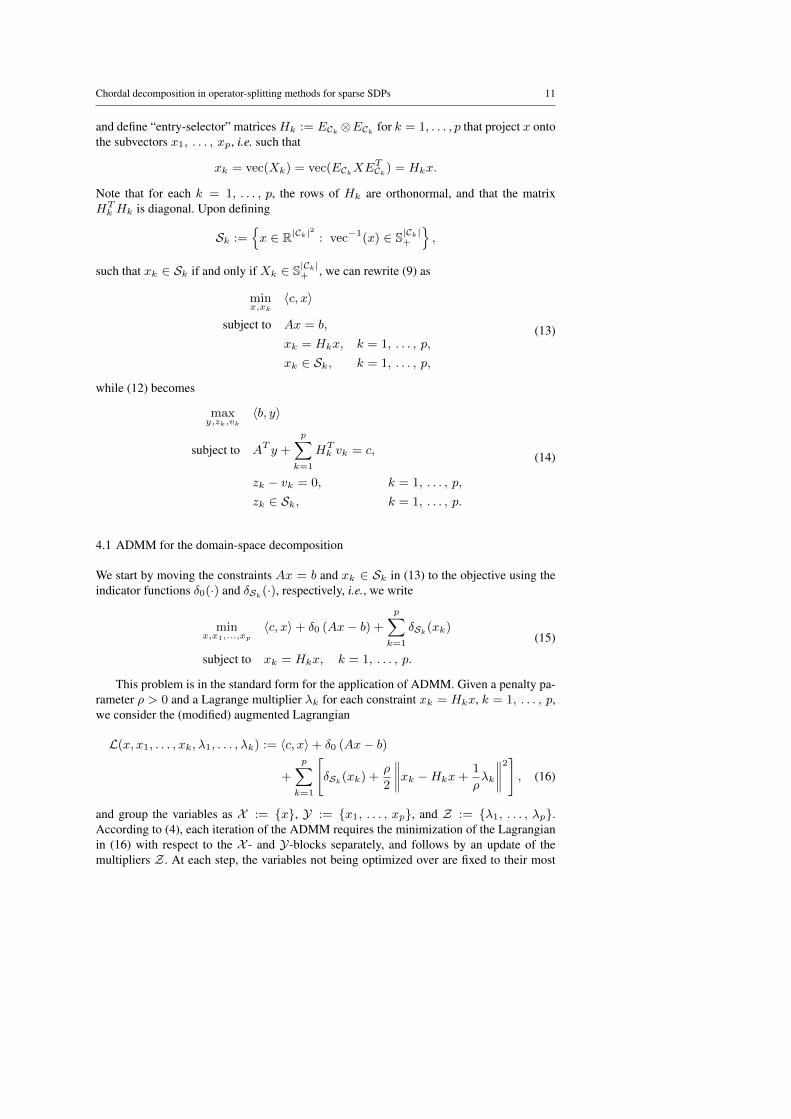
and define “entry-selector” matricesHk := ECk ⊗ECk for k = 1, . . . , p that project x ontothe subvectors x1, . . . , xp, i.e. such that

xk = vec(Xk) = vec(ECkXETCk) = Hkx.

Note that for each k = 1, . . . , p, the rows of Hk are orthonormal, and that the matrixHTk Hk is diagonal. Upon defining

Sk :={x ∈ R|Ck|

2

: vec−1(x) ∈ S|Ck|+

},

such that xk ∈ Sk if and only if Xk ∈ S|Ck|+ , we can rewrite (9) as

minx,xk

〈c, x〉

subject to Ax = b,

xk = Hkx, k = 1, . . . , p,

xk ∈ Sk, k = 1, . . . , p,

(13)

while (12) becomes

maxy,zk,vk

〈b, y〉

subject to AT y +

p∑k=1

HTk vk = c,

zk − vk = 0, k = 1, . . . , p,

zk ∈ Sk, k = 1, . . . , p.

(14)

4.1 ADMM for the domain-space decomposition

We start by moving the constraints Ax = b and xk ∈ Sk in (13) to the objective using theindicator functions δ0(·) and δSk

(·), respectively, i.e., we write

minx,x1,...,xp

〈c, x〉+ δ0 (Ax− b) +

p∑k=1

δSk(xk)

subject to xk = Hkx, k = 1, . . . , p.

(15)

This problem is in the standard form for the application of ADMM. Given a penalty pa-rameter ρ > 0 and a Lagrange multiplier λk for each constraint xk = Hkx, k = 1, . . . , p,we consider the (modified) augmented Lagrangian

L(x, x1, . . . , xk, λ1, . . . , λk) := 〈c, x〉+ δ0 (Ax− b)

+

p∑k=1

[δSk

(xk) +ρ

2

∥∥∥∥xk −Hkx+1

ρλk

∥∥∥∥2], (16)

and group the variables as X := {x}, Y := {x1, . . . , xp}, and Z := {λ1, . . . , λp}.According to (4), each iteration of the ADMM requires the minimization of the Lagrangianin (16) with respect to the X - and Y-blocks separately, and follows by an update of themultipliers Z . At each step, the variables not being optimized over are fixed to their most


current value. Note that splitting the primal variables x, x1, . . . , xp in the two blocks Xand Y defined above is essential to solving the X and Y minimization subproblems (4a)and (4b); more details will be given in Remark 3 after describing the Y-minimization stepin Section 4.1.2.

4.1.1 Minimization over X

Minimizing the augmented Lagrangian (16) overX is equivalent to the equality-constrainedquadratic program

minx

〈c, x〉+ρ

2

p∑k=1

∥∥∥∥x(n)k −Hkx+1

ρλ(n)k

∥∥∥∥2subject to Ax = b.

(17)

Letting ρy be the multiplier for the equality constraint (we scale the multiplier by ρ forconvenience), and defining

D :=

p∑k=1

HTk Hk, (18)

the optimality conditions for (17) can be written as the KKT system[D AT

A 0

] [xy

]=

[∑pk=1H

Tk

(x(n)k + ρ−1λ

(n)k

)− ρ−1c

b

]. (19)

Recalling that the product HTk Hk is a diagonal matrix for all k = 1, . . . , p we conclude

that so is D, and since A has full row rank by assumption (19) can be solved efficiently, forinstance by block elimination. In particular, eliminating x shows that the only matrix to beinverted/factorized is

AD−1AT ∈ Sm (20)

Incidentally, we note that the first-order algorithms of [29, 40] require the factorization of asimilar matrix with the same dimension. Since this matrix is the same at every iteration, itsCholesky factorization (or any other factorization of choice) can be computed and cachedbefore starting the ADMM iterations. For some families of SDPs, such as the SDP relax-ation of MaxCut problems and sum-of-squares (SOS) feasibility problems [46], the matrixAD−1AT is diagonal, so solving (19) is inexpensive even when the SDPs are very large. IffactorizingAD−1AT is too expensive, the linear system (19) can alternatively be solved byan iterative method, such as the conjugate gradient method [33].

4.1.2 Minimization over Y

Minimizing the augmented Lagrangian (16) over Y is equivalent to solving p independentconic problems of the form

minxk

∥∥∥xk −Hkx(n+1) + ρ−1λ(n)k

∥∥∥2subject to xk ∈ Sk.

(21)


In terms of the original matrix variablesX1, . . . , Xp, each of these p sub-problems amountsto a projection on a PSD cone. More precisely, if PSk

denotes the projection onto the PSDcone Sk and mat(·) = vec−1(·), we have

x(n+1)k = vec

{PSk

[mat

(Hkx

(n+1) − ρ−1λ(n)k

)]}. (22)

Since the projection PSkcan be computed with an eigenvalue decomposition, and s-

ince the size of each cone S|Ck|+ is small for typical sparse SDPs (such as SDP relaxationsof MaxCut problems), the variables x1, . . . , xp can be updated efficiently. Moreover, thecomputation can be carried out in parallel. In contrast, the algorithms for generic SDPsdeveloped in [28, 29, 40] require projections onto the original large PSD cone Sn+.

Remark 3 As anticipated in Remark 1, retaining the global variable x in the domain-spacedecomposed SDP to enforce the consensus constraints between the entries of the subvectorsx1, . . . , xp (i.e., xk = Hkx) is fundamental. In fact, it allowed us to separate the conic con-straints from the affine constraints in (13) when applying the splitting strategy of ADMM,making the minimization over Y easy to compute and parallelizable. In contrast, when x iseliminated as in the conversion method of [16, 24], the conic constraints and the affine con-straints cannot be easily decoupled when applying the first-order splitting method: in [35] aquadratic SDP had to be solved at each iteration, impeding the scalability of the algorithm.

4.1.3 Updating the multipliers Z

The final step in the n-th ADMM iteration is to update the multipliers λ1 . . . , λp with theusual gradient ascent rule: for each k = 1, . . . , p,

λ(n+1)k = λ

(n)k + ρ

(x(n+1)k −Hkx(n+1)

). (23)

This computation is cheap and easily parallelized.

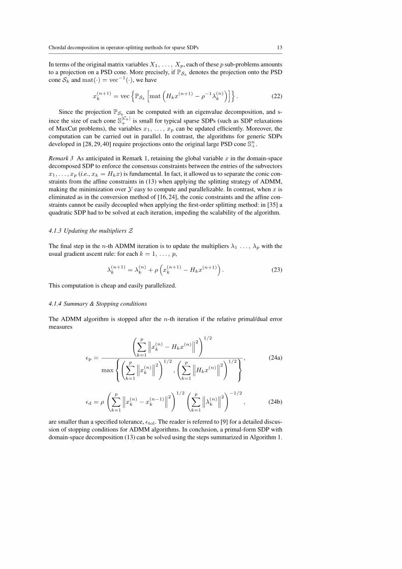
4.1.4 Summary & Stopping conditions

The ADMM algorithm is stopped after the n-th iteration if the relative primal/dual errormeasures

εp =

(p∑k=1

∥∥∥x(n)k −Hkx(n)∥∥∥2)1/2

max

(

p∑k=1

∥∥∥x(n)k

∥∥∥2)1/2

,

(p∑k=1

∥∥∥Hkx(n)∥∥∥2)1/2, (24a)

εd = ρ

(p∑k=1

∥∥∥x(n)k − x(n−1)k

∥∥∥2)1/2( p∑k=1

∥∥∥λ(n)k

∥∥∥2)−1/2

, (24b)

are smaller than a specified tolerance, εtol. The reader is referred to [9] for a detailed discus-sion of stopping conditions for ADMM algorithms. In conclusion, a primal-form SDP withdomain-space decomposition (13) can be solved using the steps summarized in Algorithm 1.


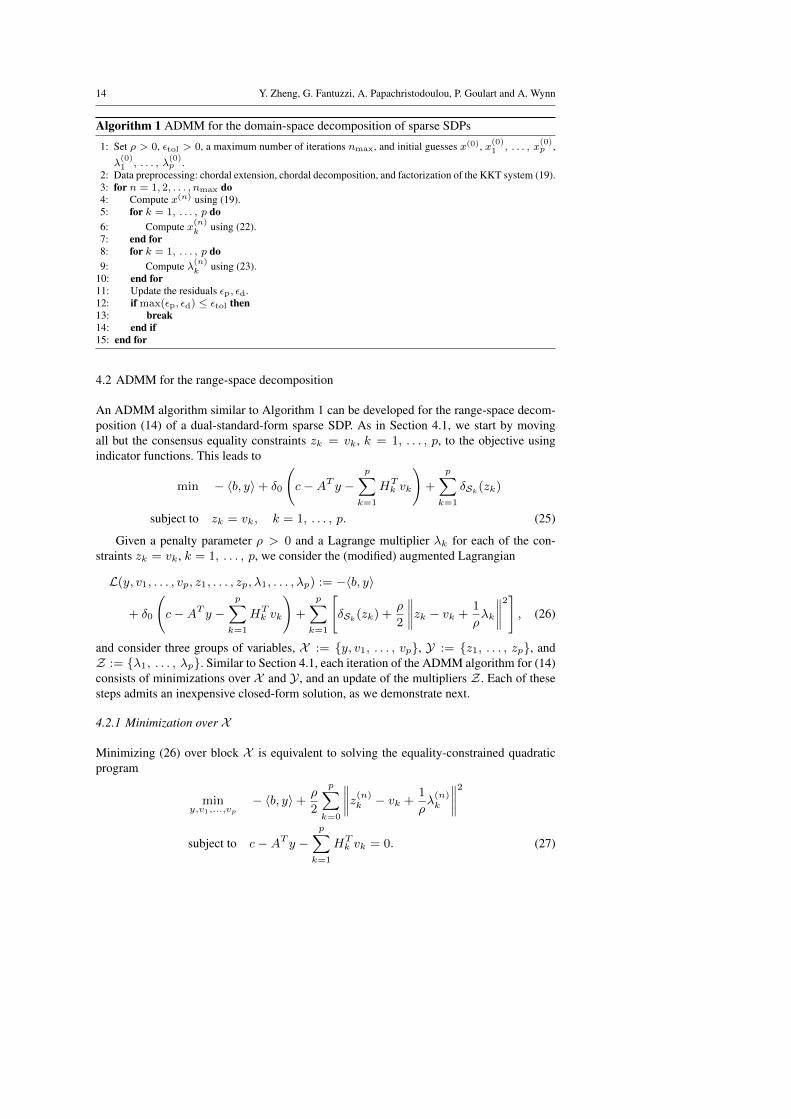
Algorithm 1 ADMM for the domain-space decomposition of sparse SDPs

1: Set ρ > 0, εtol > 0, a maximum number of iterations nmax, and initial guesses x(0), x(0)1 , . . . , x(0)p ,

λ(0)1 , . . . , λ

(0)p .

2: Data preprocessing: chordal extension, chordal decomposition, and factorization of the KKT system (19).3: for n = 1, 2, . . . , nmax do4: Compute x(n) using (19).5: for k = 1, . . . , p do6: Compute x(n)k using (22).7: end for8: for k = 1, . . . , p do9: Compute λ(n)k using (23).

10: end for11: Update the residuals εp, εd.12: if max(εp, εd) ≤ εtol then13: break14: end if15: end for

4.2 ADMM for the range-space decomposition

An ADMM algorithm similar to Algorithm 1 can be developed for the range-space decom-position (14) of a dual-standard-form sparse SDP. As in Section 4.1, we start by movingall but the consensus equality constraints zk = vk, k = 1, . . . , p, to the objective usingindicator functions. This leads to

min − 〈b, y〉+ δ0

(c−AT y −

p∑k=1

HTk vk

)+

p∑k=1

δSk(zk)

subject to zk = vk, k = 1, . . . , p. (25)

Given a penalty parameter ρ > 0 and a Lagrange multiplier λk for each of the con-straints zk = vk, k = 1, . . . , p, we consider the (modified) augmented Lagrangian

L(y, v1, . . . , vp, z1, . . . , zp, λ1, . . . , λp) := −〈b, y〉

+ δ0

(c−AT y −

p∑k=1

HTk vk

)+

p∑k=1

[δSk

(zk) +ρ

2

∥∥∥∥zk − vk +1

ρλk

∥∥∥∥2], (26)

and consider three groups of variables, X := {y, v1, . . . , vp}, Y := {z1, . . . , zp}, andZ := {λ1, . . . , λp}. Similar to Section 4.1, each iteration of the ADMM algorithm for (14)consists of minimizations over X and Y , and an update of the multipliers Z . Each of thesesteps admits an inexpensive closed-form solution, as we demonstrate next.

4.2.1 Minimization over X

Minimizing (26) over block X is equivalent to solving the equality-constrained quadraticprogram

miny,v1,...,vp

− 〈b, y〉+ρ

2

p∑k=0

∥∥∥∥z(n)k − vk +1

ρλ(n)k

∥∥∥∥2subject to c−AT y −

p∑k=1

HTk vk = 0. (27)


Let ρx be the multiplier for the equality constraint. After some algebra, the optimality con-ditions for (27) can be written as the KKT system[

D AT

A 0

] [xy

]=

[c−

∑pk=1H

Tk

(z(n)k + ρ−1λ

(n)k

)−ρ−1b

], (28)

plus a set of p uncoupled equations for the variables vk,

vk = z(n)k +

1

ρλ(n)k +Hkx, k = 1, . . . , p. (29)

The KKT system (28) is the same as (19) after rescaling x 7→ −x, y 7→ −y, c 7→ρ−1c and b 7→ ρb. Consequently, the numerical cost of these operations is the same as inSection 4.1.1, plus the cost of (29), which is cheap and can be parallelized. Moreover, as inSection 4.1.1, the factors of the coefficient matrix required to solve the KKT system (28)can be pre-computed and cached, before iterating the ADMM algorithm.

4.2.2 Minimization over Y

As in Section 4.1.2, the variables z1, . . . , zp are updated with p independent projections,

z(n+1)k = vec

{PSk

[mat

(v(n+1)k − ρ−1λ

(n)k

)]}, (30)

where PSkdenotes projection on the PSD cone S|Ck|+ . Again, these projections can be com-

puted efficiently and in parallel.

Remark 4 As anticipated in Section 3.2, introducing the set of slack variables vk and theconsensus constraints zk = vk, k = 1, . . . , p is essential to obtain an efficient algorithmfor range-space decomposed SDPs. The reason is that the splitting strategy of the ADMMdecouples the conic and affine constraints, and the conic variables can be updated using thesimple conic projection (30).

4.2.3 Updating the multipliers Z

The multipliers λk, k = 1, . . . , p, are updated (possibly in parallel) with the cheap gradientascent rule

λ(n+1)k = λ

(n)k + ρ

(z(n+1)k − v(n+1)

k

). (31)

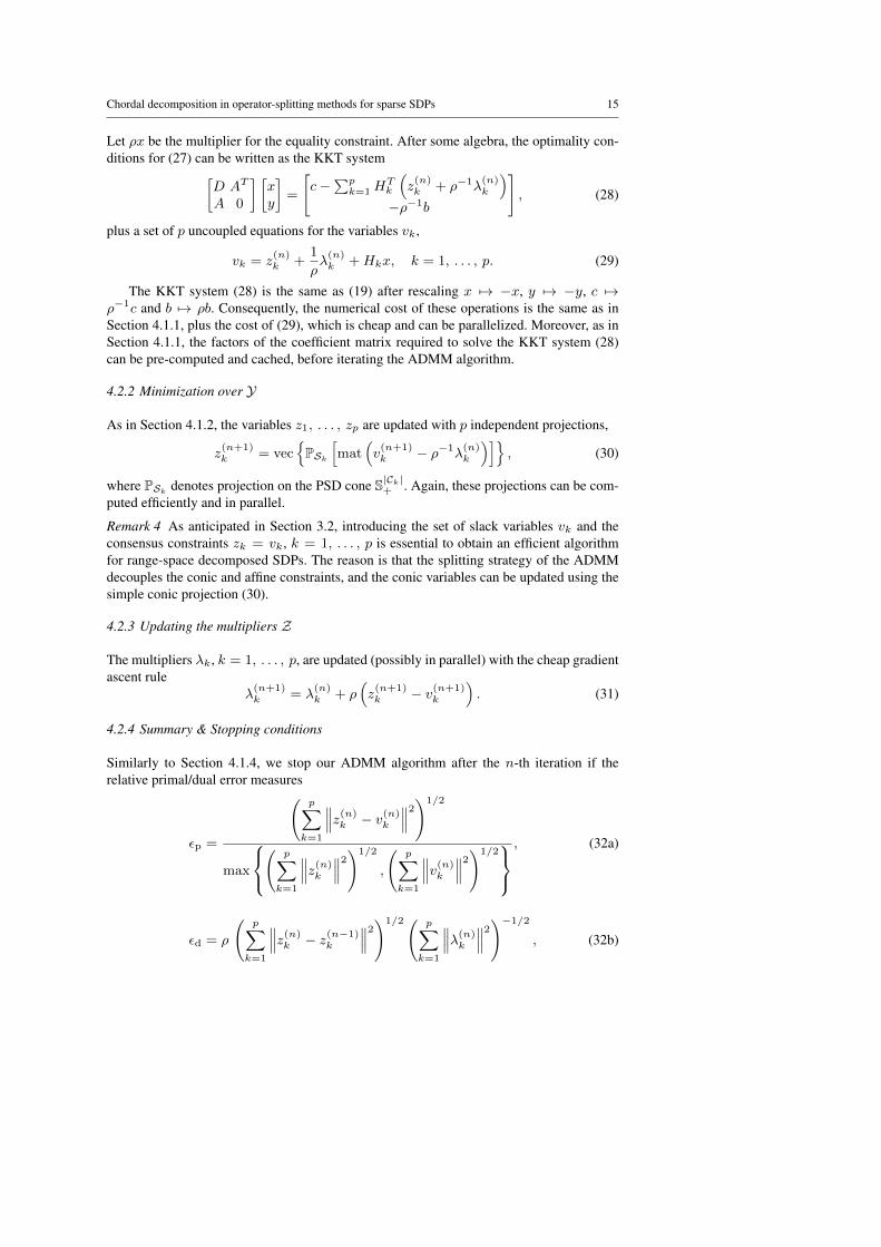
4.2.4 Summary & Stopping conditions

Similarly to Section 4.1.4, we stop our ADMM algorithm after the n-th iteration if therelative primal/dual error measures

εp =

(p∑k=1

∥∥∥z(n)k − v(n)k

∥∥∥2)1/2

max

(

p∑k=1

∥∥∥z(n)k

∥∥∥2)1/2

,

(p∑k=1

∥∥∥v(n)k

∥∥∥2)1/2, (32a)

εd = ρ

(p∑k=1

∥∥∥z(n)k − z(n−1)k

∥∥∥2)1/2( p∑k=1

∥∥∥λ(n)k

∥∥∥2)−1/2

, (32b)


Algorithm 2 ADMM for dual form SDPs with range-space decomposition

1: Set ρ > 0, εtol > 0, a maximum number of iterations nmax and initial guesses y(0), z(0)1 , . . . , z(0)p ,

λ(0)1 , . . . , λ

(0)p .

2: Data preprocessing: chordal extension, chordal decomposition, and factorization of the KKT system (28).3: for n = 1, 2, . . . , nmax do4: for k = 1, . . . , p do5: Compute z(n)k using (30).6: end for7: Compute y(n), x using (27).8: for k = 1, . . . , p do9: Compute v(n)k using (29)

10: Compute λ(n)k using (33) (no cost).11: end for12: Update the residuals εp and εd.13: if max(εp, εd) ≤ εtol then14: break15: end if16: end for

are smaller than a specified tolerance, εtol. The ADMM algorithm to solve the range-spacedecomposition (14) of a dual-form sparse SDP is summarized in Algorithm 2.

4.3 Equivalence between the primal and dual ADMM algorithms

Since the computational cost of (29) is the same as (23), all ADMM iterations for the dual-form SDP with range-space decomposition (14) have the same cost as those for the primal-form SDP with domain-space decomposition (13), plus the cost of (31). However, if oneminimizes the dual augmented Lagrangian (26) over z1, . . . , zp before minimizing it overy, v1, . . . , vp, then (29) can be used to simplify the multiplier update equations to

λ(n+1)k = ρHkx

(n+1), k = 1, . . . , p. (33)

Given that the products H1x, . . . ,Hpx have already been computed to update v1, . . . , vpin (29), updating the multipliers λ1, . . . , λp requires only a scaling operation. Recallingthat (19) and (28) are scaled versions of the same KKT system, after swapping the orderof the minimization, the ADMM algorithms for the primal and dual standard form SDPscan be considered as scaled versions of each other; see Fig. 4 for an illustration. In fact, theequivalence between ADMM algorithms for the original (i.e., before chordal decomposition)primal and dual SDPs was already noted in [41].

Remark 5 Although the iterates of Algorithm 1 and Algorithm 2 are the same up to scaling,the convergence performance of these two algorithms differ in practice because first-ordermethods are sensitive to the scaling of the problem data and of the iterates.

5 Homogeneous self-dual embedding of domain- and range-space decomposed SDPs

Algorithms 1 and 2, as well as other first-order algorithms that exploit chordal sparsi-ty [23, 27, 35], can solve feasible problems, but cannot detect infeasibility in their current


formulation. Although some recent ADMM methods reslove this issue [5, 25], an elegan-t way to deal with an infeasible primal-dual pair of SDPs—which we pursue here—is tosolve their homogeneous self-dual embedding (HSDE) [44].

The essence of the HSDE method is to search for a non-zero point in the intersection ofa convex cone and a linear space; this is non-empty because it always contains the origin,meaning that the problem is always feasible. Given such a non-zero point, one can eitherrecover optimal primal and dual solutions of the original pair of optimization problems,or construct a certificate of primal or dual infeasibility. HSDEs have been widely used todevelop IPMs for SDPs [34, 43], and more recently O’Donoghue et al. have proposed anoperator-splitting method to solve the HSDE of general conic programs [29].

In this section, we formulate the HSDE of the domain- and range-space decomposedSDPs (13) and (14), which is a primal-dual pair of SDPs. We also apply ADMM to solvethis HSDE; in particular, we extend the algorithm of [29] to exploit chordal sparsity withoutincreasing its computational cost (at least to leading order) compared to Algorithms 1 and 2.

5.1 Homogeneous self-dual embedding

To simplify the formulation of the HSDE of the decomposed (vectorized) SDPs (13) and (14),we let S := S1 × · · · × Sp be the direct product of all semidefinite cones and define

s :=

x1...xp

, z :=

z1...zp

, v :=

v1...vp

, H :=

H1

...Hp

.When strong duality holds, the tuple (x∗, s∗, y∗, v∗, z∗) is optimal if and only if all of

the following conditions hold:

1. (x∗, s∗) is primal feasible, i.e., Ax∗ = b, s∗ = Hx∗, and s∗ ∈ S. For reasons that willbecome apparent below, we introduce slack variables r∗ = 0 andw∗ = 0 of appropriatedimensions and rewrite these conditions as

Ax∗ − r∗ = b, s∗ + w∗ = Hx∗, s∗ ∈ S, r∗ = 0, w∗ = 0. (34)

2. (y∗, v∗, z∗) is dual feasible, i.e., AT y∗ + HT v∗ = c, z∗ = v∗, and z∗ ∈ S. Again, itis convenient to introduce a slack variable h∗ = 0 of appropriate size and write

AT y∗ +HT v∗ + h∗ = c, z∗ − v∗ = 0, z∗ ∈ S, h∗ = 0. (35)

3. The duality gap is zero, i.e.cTx∗ − bT y∗ = 0. (36)

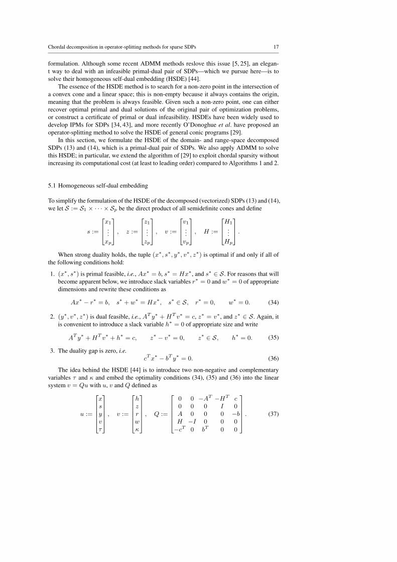
The idea behind the HSDE [44] is to introduce two non-negative and complementaryvariables τ and κ and embed the optimality conditions (34), (35) and (36) into the linearsystem v = Qu with u, v and Q defined as

u :=

xsyvτ

, v :=

hzrwκ

, Q :=

0 0 −AT −HT c0 0 0 I 0A 0 0 0 −bH −I 0 0 0

−cT 0 bT 0 0

. (37)


Any nonzero solution of this embedding can be used to recover an optimal solution for (9)and (12), or provide a certificate for primal or dual infeasibility, depending on the values ofτ and κ; details are omitted for brevity, and the interested reader is referred to [29].

The decomposed primal-dual pair of (vectorized) SDPs (13)-(14) can therefore be recastas the self-dual conic feasibility problem

find (u, v)

subject to v = Qu,

(u, v) ∈ K ×K∗,(38)

where, writing nd =∑pk=1 |Ck|

2 for brevity, K := Rn2

×S ×Rm ×Rnd ×R+ is a coneand K∗ := {0}n

2

× S × {0}m × {0}nd × R+ is its dual.

5.2 A simplified ADMM algorithm

The feasibility problem (38) is in a form suitable for the application of ADMM, and more-over steps (4a)-(4c) can be greatly simplified by virtue of its self-dual character [29]. Specifi-cally, the n-th iteration of the simplified ADMM algorithm for (38) proposed in [29] consistsof the following three steps, where PK denotes projection onto the cone K:

u(n+1) = (I +Q)−1(u(n) + v(n)

), (39a)

u(n+1) = PK(u(n+1) − v(n)

), (39b)

v(n+1) = v(n) − u(n+1) + u(n+1). (39c)

Note that (39b) is inexpensive, since K is the cartesian product of simple cones (zero,free and non-negative cones) and small PSD cones, and can be efficiently carried out in par-allel. The third step is also computationally inexpensive and parallelizable. On the contrary,even when the preferred factorization of I + Q (or its inverse) is cached before startingthe iterations a direct implementation of (39a) may require substantial computational effortbecause

Q ∈ Sn2+2nd+m+1

is a very large matrix (e.g., n2 + 2nd + m + 1 = 2360900 for the instance of rs365 inSection 6.3, which would take over 104 GB to store Q as a dense double-precision matrix).Yet, as we can see in (37), Q is highly structured and sparse, and these properties can beexploited to speed up step (39a) using a series of block-eliminations and the matrix inversionlemma [10, Section C.4.3].

5.2.1 Solving the “outer” linear system

The affine projection step (39a) requires the solution of a linear system (which we refer toas the “outer” system for reasons that will become clear below) of the form[

M ζ

−ζT 1

] [u1u2

]=

[ω1

ω2

], (40)


where

M :=

[I AT

−A I

], ζ :=

[c

b

], A :=

[−A 0−H I

], c :=

[c0

], b :=

[−b0

](41)

and we have split

u(n) + v(n) =

[ω1

ω2

]. (42)

Note that u2 and ω2 are scalars. After one step of block elimination in (40) we obtain

(M + ζζT )u1 = ω1 − ω2ζ, (43)

u2 = ω2 + ζT u1. (44)

Moreover, applying the matrix inversion lemma [10, Section C.4.3] to (43) shows that

u1 =

[I − (M−1ζ)ζT

1 + ζT (M−1ζ)

]M−1 (ω1 − ω2ζ) . (45)

Note that the vector M−1ζ and the scalar 1 + ζT (M−1ζ) depend only on the problemdata, and can be computed before starting the ADMM iterations (sinceM is quasi-definite itcan be inverted, and any symmetric matrix obtained as a permutation ofM admits an LDLT

factorization). Instead, recalling from (42) that ω1 − ω2ζ changes at each iteration becauseit depends on the iterates u(n) and v(n), the vector M−1 (ω1 − ω2ζ) must be computed ateach iteration. Consequently, computing u1 and u2 requires the solution of an “inner” linearsystem for the vector M−1 (ω1 − ω2ζ), followed by inexpensive vector inner products andscalar-vector operations in (45) and (44).

5.2.2 Solving the “inner” linear system

Recalling the definition of M from (41), the “inner” linear system to calculate u1 in (45)has the form [

I AT

−A I

] [σ1σ2

]=

[ν1ν2

], (46)

where σ1 and σ2 are the unknowns and represent suitable partitions of the vectorM−1(ω1−ω2ζ) in (45) (which is to be calculated), and where we have split

ω1 − ω2ζ =

[ν1ν2

].

Applying block elimination to remove σ1 from the second equation in (46), we obtain

σ1 = ν1 − ATσ2, (47)

(I + AAT )σ2 = Aν1 + ν2. (48)

Recalling the definition of A and recognizing that

D = HTH =

p∑k=1

HTk Hk


is a diagonal matrix, as already noted in Section 4.1.1, we also have

I + AAT =

[(I +D +ATA) −HT

−H 2I

]. (49)

Block elimination can therefore be used once again to solve (48), and simple algebraicmanipulations show that the only matrix to be factorized (or inverted) is

I +1

2D +ATA ∈ Sn

2

. (50)

Note that this matrix depends only on the problem data and the chordal decomposition, soit can be factorized/inverted before starting the ADMM iterations. In addition, it is of the“diagonal plus low rank” form becauseA ∈ Rm×n

2

withm < n2 (in fact, oftenm� n2).This means that the matrix inversion lemma can be used to reduce the size of the matrix tofactorize/invert even further: letting P = I + 1

2D be the diagonal part of (50), we have

(P +ATA)−1 = P−1 − P−1AT (I +AP−1AT )−1AP−1.

In summary, after a series of block eliminations and applications of the matrix inversionlemma, step (39a) of the ADMM algorithm for (38) only requires the solution of an m×mlinear system of equations with coefficient matrix

I +A

(I +

1

2D

)−1

AT ∈ Sm, (51)

plus a sequence of matrix-vector, vector-vector, and scalar-vector multiplications.

5.2.3 Stopping conditions

The ADMM algorithm described in the previous section can be stopped after the n-th iter-ation if a primal-dual optimal solution or a certificate of primal and/or dual infeasibility isfound, up to a specified tolerance εtol. As noted in [29], rather than checking the convergenceof the variables u and v, it is desirable to check the convergence of the original primal anddual SDP variables using the primal and dual residual error measures normally considered ininterior-point algorithms [34]. For this reason, we employ different stopping conditions thanthose used in Algorithms 1 and 2, which we define below. As for our notation, we denotethe entries of u in (37) that correspond to x, y, v, τ , respectively, by ux, uy, uv, uτ .

If at the n-th iteration of the ADMM algorithm u(n)τ > 0 we take

x(n) =u(n)x

u(n)τ

, y(n) =u(n)y

u(n)τ

, z(n) =u(n)v

u(n)τ

,

as the candidate primal-dual points. We terminate the algorithm if the relative primal resid-ual, dual residual and duality gap, defined as

εp =Ax(n) − b1 + ‖b‖2

, εd =AT y(n) + z(n) − c

1 + ‖c‖2, εgap =

cTx(n) − bT y(n)

1 + ‖cTx(n)‖2 + ‖bT y(n)‖2,

are smaller than εtol. If, instead, u(n)τ = 0, we terminate the algorithm if

max

{‖Au(n)x ‖2 +

cTu(n)x

‖c‖2εtol, ‖ATu(n)y + z(n)‖2 −

bTu(n)y

‖b‖2εtol

}≤ 0. (52)


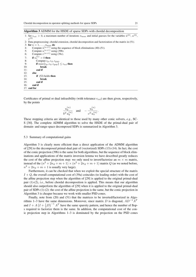
Algorithm 3 ADMM for the HSDE of sparse SDPs with chordal decomposition1: Set εtol > 0, a maximum number of iterations nmax and initial guesses for the variables u(0), u(0),v(0)

2: Data preprocessing: chordal extension, chordal decomposition and factorization of the matrix in (51).3: for n = 1, . . . , nmax do4: Compute u(n+1) using the sequence of block eliminations (40)-(51).5: Compute u(n+1) using (39b).6: Compute v(n+1) using (39c).7: if u(n)τ > 0 then8: Compute εp, εd, εgap.9: if max{εp, εd, εgap} ≤ εtol then

10: break11: end if12: else13: if (52) holds then14: break15: end if16: end if17: end for

Certificates of primal or dual infeasibility (with tolerance εtol) are then given, respectively,by the points

u(n)y

bTu(n)y

and − u(n)x

cTu(n)x

.

These stopping criteria are identical to those used by many other conic solvers, e.g., SC-S [30]. The complete ADMM algorithm to solve the HSDE of the primal-dual pair ofdomain- and range-space decomposed SDPs is summarized in Algorithm 3.

5.3 Summary of computational gains

Algorithm 3 is clearly more efficient than a direct application of the ADMM algorithmof [29] to the decomposed primal-dual pair of (vectorized) SDPs (13)-(14). In fact, the costof the conic projection (39b) is the same for both algorithms, but the sequence of block elim-inations and applications of the matrix inversion lemma we have described greatly reducesthe cost of the affine projection step: we only need to invert/factorize an m × m matrix,instead of the (n2 + 2nd +m+ 1)× (n2 + 2nd +m+ 1) matrix Q (as we noted before,n2 + 2nd +m+ 1 is usually very large).

Furthermore, it can be checked that when we exploit the special structure of the matrixI + Q, the overall computational cost of (39a) coincides (to leading order) with the cost ofthe affine projection step when the algorithm of [29] is applied to the original primal-dualpair (1)-(2), i.e., before chordal decomposition is applied. This means that our algorithmshould also outperform the algorithm of [29] when it is applied to the original primal-dualpair of SDPs (1)-(2): the cost of the affine projection is the same, but the conic projection inAlgorithm 3 is cheaper because we work with smaller PSD cones.

Finally, note from (20) and (51) that the matrices to be inverted/factorized in Algo-rithms 1–3 have the same dimensions. Moreover, since matrix D is diagonal, AD−1AT

and I + A(I + 1

2D)−1

AT have the same sparsity pattern, and hence the number of flop-s required to factorize them is the same. In addition, the computational cost of the con-ic projection step in Algorithms 1–3 is dominated by the projection on the PSD cones


S|Ck|, k = 1, . . . , p, which are the same in all three algorithms (they are determined bythe chordal decomposition of the aggregate sparsity pattern of the original problem). Con-sequently, each iteration of our ADMM algorithm for the HSDE formulation has the sameleading order cost as applying the ADMM to the primal and dual problem alone, with themajor advantage of being able to detect infeasibility.

6 Implementation and numerical experiments

We implemented Algorithms 1-3 in an open-source MATLAB solver which we call CDCS(Cone Decomposition Conic Solver). We refer to our implementation of Algorithms 1-3as CDCS-primal, CDCS-dual and CDCS-hsde, respectively. This section briefly describesCDCS, and presents numerical results of some sparse SDPs from SDPLIB [7], some largeand sparse SDPs with nonchordal sparsity patterns from [4], and randomly generated SDPswith block-arrow sparsity pattern. Such problems have also been used as benchmarks in [4,35].

In order to highlight the advantages of chordal decomposition, first-order algorithm-s, and their combination, the three algorithms in CDCS are compared to the interior-pointsolver SeDuMi [34], and to the single-threaded direct implementation of the first-order algo-rithm of [29] provided by the conic solver SCS [30]. All solvers were called with terminationtolerance εtol = 10−3, number of iterations limited to 2 000, and their default remainingparameters. The purpose of comparing CDCS to a low-accuracy IPM is to demonstrate theadvantages of combining FOMs with chordal decomposition, while a comparison to thehigh-performance first-order conic solver SCS highlights the advantages of chordal decom-position alone. Accurate solutions (εtol = 10−8) were also computed using SeDuMi; thesecan be considered “exact”, and used to assess how far the solution returned by CDCS is fromoptimality. All experiments were carried out on a PC with a 2.8 GHz Intel Core i7 CPU and8GB of RAM.

6.1 CDCS

To the best of our knowledge, CDCS is the first open-source first-order conic solver thatexploits chordal decomposition for the PSD cones and is able to handle infeasible problems.Cartesian products of the following cones are supported: the cone of free variables Rn, thenon-negative orthant Rn+, second-order cones, and PSD cones. The current implementationis written in MATLAB and can be downloaded from

https://github.com/oxfordcontrol/cdcs .Note that although many steps of Algorithms 1–3 can be carried out in parallel, our im-plementation is sequential. Interfaces with the optimization toolboxes YALMIP [26] andSOSTOOLS [31] are also available.

6.1.1 Implementation details

CDCS applies chordal decomposition to all PSD cones. Following [38], the sparsity patternof each PSD cone is chordal extended using the MATLAB function chol to compute asymbolic Cholesky factorization of the approximate minimum-degree permutation of thecone’s adjacency matrix, returned by the MATLAB function symamd. The maximal cliquesof the chordal extension are then computed using a .mex function from SparseCoLO [15].

https://github.com/oxfordcontrol/cdcs


As far as the steps of our ADMM algorithms are concerned, projections onto the PSDcone are performed using the MATLAB routine eig, while projections onto other supportedcones only use vector operations. The Cholesky factors of the m ×m linear system coef-ficient matrix (permuted using symamd) are cached before starting the ADMM iterations.The permuted linear system is solved at each iteration using the routines cs lsolve andcs ltsolve from the CSparse library [12].

6.1.2 Adaptive penalty strategy

While the ADMM algorithms proposed in the previous sections converge independently ofthe choice of penalty parameter ρ, in practice its value strongly influences the number ofiterations required for convergence. Unfortunately, analytic results for the optimal choiceof ρ are not available except for very special problems [18, 32]. Consequently, in order toimprove the convergence rate and make performance less dependent on the choice of ρ,CDCS employs the dynamic adaptive rule

ρk+1 =

µincr ρ

k if ‖εkp‖2 ≥ ν‖εkd‖2ρk/µdecr if ‖εkd‖2 ≥ ν‖εkp‖2ρk otherwise.

,

Here, εkp and εkd are the primal and dual residuals at the k-th iteration, while µincr, µdecr and νare parameters no smaller than 1. Note that since ρ does not enter any of the matrices beingfactorized/inverted, updating its value is computationally cheap.

The idea of the rule above is to adapt ρ to balance the convergence of the primal anddual residuals to zero; more details can be found in [9, Section 3.4.1]. Typical choices forthe parameters (the default in CDCS) are µincr = µdecr = 2 and ν = 10 [9].

6.1.3 Scaling the problem data

The relative scaling of the problem data also affects the convergence rate of ADMM algo-rithms. CDCS scales the problem data after the chordal decomposition step using a strategysimilar to [29]. In particular, the decomposed SDPs (13) and (14) can be rewritten as:

minx

cT x

s.t. Ax = b

x ∈ Rn2

×K,

maxy,z

bT y

s.t. AT y + z = c

z ∈ {0}n2

× K∗(53a,b)

where

x =

[xxh

], c =

[c0

], b =

[b0

], A =

[A 0H −I

].

CDCS solves the scaled problems

minx

σ(Dc)T x

s.t. EADx = ρEb

x ∈ Rn2

×K,

maxy,z

ρ(Eb)T y

s.t. DATEy + z = σDc

z ∈ {0}n2

×K∗,

(54a,b)


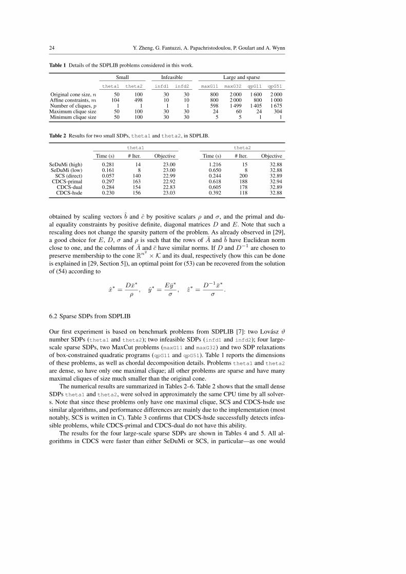
Table 1 Details of the SDPLIB problems considered in this work.

Small Infeasible Large and sparse

theta1 theta2 infd1 infd2 maxG11 maxG32 qpG11 qpG51

Original cone size, n 50 100 30 30 800 2 000 1 600 2 000Affine constraints, m 104 498 10 10 800 2 000 800 1 000Number of cliques, p 1 1 1 1 598 1 499 1 405 1 675Maximum clique size 50 100 30 30 24 60 24 304Minimum clique size 50 100 30 30 5 5 1 1

Table 2 Results for two small SDPs, theta1 and theta2, in SDPLIB.

theta1 theta2

Time (s) # Iter. Objective Time (s) # Iter. Objective

SeDuMi (high) 0.281 14 23.00 1.216 15 32.88SeDuMi (low) 0.161 8 23.00 0.650 8 32.88

SCS (direct) 0.057 140 22.99 0.244 200 32.89CDCS-primal 0.297 163 22.92 0.618 188 32.94

CDCS-dual 0.284 154 22.83 0,605 178 32.89CDCS-hsde 0.230 156 23.03 0.392 118 32.88

obtained by scaling vectors b and c by positive scalars ρ and σ, and the primal and du-al equality constraints by positive definite, diagonal matrices D and E. Note that such arescaling does not change the sparsity pattern of the problem. As already observed in [29],a good choice for E, D, σ and ρ is such that the rows of A and b have Euclidean normclose to one, and the columns of A and c have similar norms. If D and D−1 are chosen topreserve membership to the cone Rn

2

×K and its dual, respectively (how this can be doneis explained in [29, Section 5]), an optimal point for (53) can be recovered from the solutionof (54) according to

x∗ =Dx∗

ρ, y∗ =

Ey∗

σ, z∗ =

D−1x∗

σ.

6.2 Sparse SDPs from SDPLIB

Our first experiment is based on benchmark problems from SDPLIB [7]: two Lovasz ϑnumber SDPs (theta1 and theta2); two infeasible SDPs (infd1 and infd2); four large-scale sparse SDPs, two MaxCut problems (maxG11 and maxG32) and two SDP relaxationsof box-constrained quadratic programs (qpG11 and qpG51). Table 1 reports the dimensionsof these problems, as well as chordal decomposition details. Problems theta1 and theta2

are dense, so have only one maximal clique; all other problems are sparse and have manymaximal cliques of size much smaller than the original cone.

The numerical results are summarized in Tables 2–6. Table 2 shows that the small denseSDPs theta1 and theta2, were solved in approximately the same CPU time by all solver-s. Note that since these problems only have one maximal clique, SCS and CDCS-hsde usesimilar algorithms, and performance differences are mainly due to the implementation (mostnotably, SCS is written in C). Table 3 confirms that CDCS-hsde successfully detects infea-sible problems, while CDCS-primal and CDCS-dual do not have this ability.

The results for the four large-scale sparse SDPs are shown in Tables 4 and 5. All al-gorithms in CDCS were faster than either SeDuMi or SCS, in particular—as one would


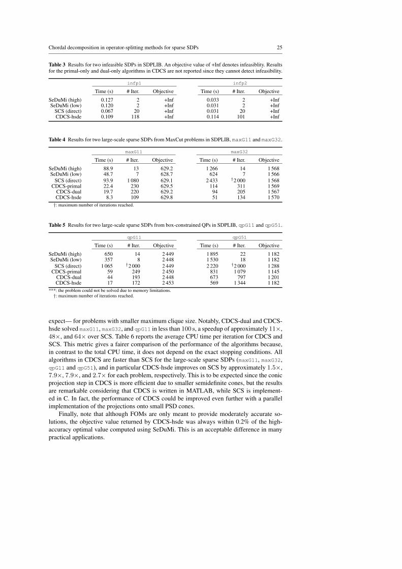
Table 3 Results for two infeasible SDPs in SDPLIB. An objective value of +Inf denotes infeasiblity. Resultsfor the primal-only and dual-only algorithms in CDCS are not reported since they cannot detect infeasibility.

infp1 infp2


SeDuMi (high) 0.127 2 +Inf 0.033 2 +InfSeDuMi (low) 0.120 2 +Inf 0.031 2 +Inf

SCS (direct) 0.067 20 +Inf 0.031 20 +InfCDCS-hsde 0.109 118 +Inf 0.114 101 +Inf

Table 4 Results for two large-scale sparse SDPs from MaxCut problems in SDPLIB, maxG11 and maxG32.

maxG11 maxG32


SeDuMi (high) 88.9 13 629.2 1 266 14 1 568SeDuMi (low) 48.7 7 628.7 624 7 1 566

SCS (direct) 93.9 1 080 629.1 2 433 †2 000 1 568CDCS-primal 22.4 230 629.5 114 311 1 569

CDCS-dual 19.7 220 629.2 94 205 1 567CDCS-hsde 8.3 109 629.8 51 134 1 570†: maximum number of iterations reached.

Table 5 Results for two large-scale sparse SDPs from box-constrained QPs in SDPLIB, qpG11 and qpG51.

qpG11 qpG51


SeDuMi (high) 650 14 2 449 1 895 22 1 182SeDuMi (low) 357 8 2 448 1 530 18 1 182

SCS (direct) 1 065 †2 000 2 449 2 220 †2 000 1 288CDCS-primal 59 249 2 450 831 1 079 1 145

CDCS-dual 44 193 2 448 673 797 1 201CDCS-hsde 17 172 2 453 569 1 344 1 182

***: the problem could not be solved due to memory limitations.†: maximum number of iterations reached.

expect— for problems with smaller maximum clique size. Notably, CDCS-dual and CDCS-hsde solved maxG11, maxG32, and qpG11 in less than 100 s, a speedup of approximately 11×,48×, and 64× over SCS. Table 6 reports the average CPU time per iteration for CDCS andSCS. This metric gives a fairer comparison of the performance of the algorithms because,in contrast to the total CPU time, it does not depend on the exact stopping conditions. Allalgorithms in CDCS are faster than SCS for the large-scale sparse SDPs (maxG11, maxG32,qpG11 and qpG51), and in particular CDCS-hsde improves on SCS by approximately 1.5×,7.9×, 7.9×, and 2.7× for each problem, respectively. This is to be expected since the conicprojection step in CDCS is more efficient due to smaller semidefinite cones, but the resultsare remarkable considering that CDCS is written in MATLAB, while SCS is implement-ed in C. In fact, the performance of CDCS could be improved even further with a parallelimplementation of the projections onto small PSD cones.

Finally, note that although FOMs are only meant to provide moderately accurate so-lutions, the objective value returned by CDCS-hsde was always within 0.2% of the high-accuracy optimal value computed using SeDuMi. This is an acceptable difference in manypractical applications.


Table 6 Average CPU time per iteration (in seconds) for the SDPs from SDPLIB tested in this work.

theta1 theta2 maxG11 maxG32 qpG11 qpG51

SCS (direct) 4.0×10−4 1.2×10−3 0.087 1.216 0.532 1.110CDCS-primal 1.8×10−3 3.3×10−3 0.079 0.194 0.210 0.758

CDCS-dual 1.8×10−3 3.4×10−3 0.074 0.196 0.191 0.829CDCS-hsde 1.5×10−3 3.3×10−3 0.059 0.153 0.067 0.417

(a) rs35 (b) rs200 (c) rs228

(d) rs365 (e) rs1555 (f) rs1907

Fig. 5 Aggregate sparsity patterns of the nonchordal SDPs in [4]; see Table 7 for the matrix dimensions.

Table 7 Summary of chordal decomposition for the chordal extensions of the nonchordal SDPs form [4].

rs35 rs200 rs228 rs365 rs1555 rs1907

Original cone size, n 2003 3025 1919 4704 7479 5357Affine constraints, m 200 200 200 200 200 200Number of cliques, p 588 1635 783 1244 6912 611Maximum clique size 418 102 92 322 187 285Minimum clique size 5 4 3 6 2 7

6.3 Nonchordal SDPs

In our second experiment, we solved six large-scale SDPs with nonchordal sparsity patternsform [4]: rs35, rs200, rs228, rs365, rs1555, and rs1907. The aggregate sparsity patternsof these problems, illustrated in Fig. 5, come from the University of Florida Sparse MatrixCollection [13]. Table 7 demonstrates that all six sparsity patterns admit chordal extensionswith maximum cliques that are much smaller than the original cone.

The numerical results are presented in Table 8 and Table 9. For all problems, the algo-rithms in CDCS (primal, dual and hsde) are all much faster than either SCS or SeDuMi.For the largest instance, rs1555, CDCS-hsde returned successfully winthin 20 minutes, 100times faster than SCS, which stopped after 38 hours having reached the maximum number ofiterations without meeting the convergence tolerance. In fact, SCS never terminates succes-fully, while the objective value returned by CDCS is always within 2% of the high-accuracysolutions returned by SeDuMi (when this could be computed).


Table 8 Results for large-scale SDPs with nonchordal sparsity patterns form [4].

rs35 rs200


SeDuMi (high) 1 391 17 25.33 4 451 17 99.74SeDuMi (low) 986 11 25.34 2 223 8 99.73

SCS (direct) 2 378 †2 000 25.08 9 697 †2 000 81.87CDCS-primal 597 379 25.27 192 577 99.61

CDCS-dual 426 245 25.53 131 353 99.72CDCS-hsde 299 265 25.94 79 256 98.56

rs228 rs365


SeDuMi (high) 1 655 21 64.71 *** *** ***SeDuMi (low) 809 10 64.80 *** *** ***

SCS (direct) 2 338 †2 000 62.06 34 497 †2 000 44.02CDCS-primal 111 400 64.65 541 401 63.37

CDCS-dual 100 341 64.76 417 265 63.69CDCS-hsde 38 130 64.71 272 269 63.12

rs1555 rs1907


SeDuMi (high) *** *** *** *** *** ***SeDuMi (low) *** *** *** *** *** ***

SCS (direct) 139 314 †2 000 34.20 50 047 †2 000 45.89CDCS-primal 3 641 †2 000 61.22 572 349 62.87

CDCS-dual 779 317 69.54 466 252 63.30CDCS-hsde 1 172 1 124 60.26 206 148 63.09

***: the problem could not be solved due to memory limitations.†: maximum number of iterations reached.

Table 9 Average CPU time per ADMM iteration (in seconds) for some SDPs with nonchordal sparsity patternform [4].

rs35 rs200 rs228 rs365 rs1555 rs1907

SCS (direct) 1.188 4.847 1.169 17.250 69.590 25.240CDCS-primal 1.540 0.288 0.250 1.226 1.682 1.391

CDCS-dual 1.680 0.297 0.260 1.334 1.577 1.520CDCS-hsde 1.082 0.236 0.233 0.830 0.934 0.954

The average CPU time per iteration in CDCS-hsde is also 20×, 21×, 26×, and 75×faster than SCS, respectively, for problems rs200, rs365, rs1907, and rs1555. In addition,the results show that the average CPU time per iteration for CDCS (primal, dual, and hs-de) is independent of the original problem size and, perhaps not unexpectedly, it seems todepend mainly on the dimension of the largest clique. In fact, in all of our algorithms thecomplexity of the conic projection—which dictates the overall complexity when m is fixedto a moderate value like in the examples presented here—is determined by the size of thelargest maximal clique, not the size of the cone in the original problem.

6.4 Random SDPs with block-arrow patterns

In our last experiment, we consider randomly generated SDPs with the block-arrow aggre-gate sparsity pattern illiustrated in Figure 6. Such a sparsity pattern, used as a benchmarkcase in [4, 35], is chordal. Its parameters are: the number of blocks, l; the block size, d; and


l blocks

d

d

h

h

Fig. 6 Block-arrow sparsity pattern (dots indicate repeating diagonal blocks). The parameters are: the numberof blocks, l; block size, d; the width of the arrow head, h.

400 600 1000 2000 3500

Number of constraints, m

100

101

102

103

104

Tim

e(s)

10 20 50 100 150

Number of blocks, l

100

101

102

103

104

Tim

e(s)

5 10 15 20 25 30

Size of each block, d

100

101

102

103

104

Tim

e(s)

SeDuMi (high) SeDuMi (low) SCS (direct) CDCS-primal CDCS-dual CDCS-hsde

Fig. 7 CPU time for SDPs with block-arrow patterns. Left to right: varying number of constraints; varyingnumber of blocks; varying block size.

the size of the arrow head, h. The final parameter in our randomly generated SDPs is thenumber of constraints, m. Here, we present results for the following cases:

1. Fix l = 40, d = 10, h = 20, and vary m;2. Fix m = 1000, d = 10, h = 20, and vary l;3. Fix l = 40, h = 10, m = 1000, and vary d.

The CPU times for the different solvers considered in this work are shown in Figure 7.In all three test scenarios, CDCS is more than 10 times faster than SeDuMi even when a lowtolerance is used, and on average it is also faster than SCS. In addition, we observed thatthe optimal value returned by all algorithms in CDCS (primal, dual and hsde) was alwayswithin 0.1% of the high-accuracy value returned by SeDuMi, which can be considered to benegligible in practice.

7 Conclusion

In this paper, we have presented a conversion framework for large-scale SDPs characterizedby chordal sparsity. This framework is analogous to the conversion techniques for IPMsof [16, 24], but is more suitable for the application of FOMs. We have then developed ef-ficient ADMM algorithms for sparse SDPs in either primal or dual standard form, and fortheir homogeneous self-dual embedding. In all cases, a single iteration of our ADMM al-gorithms only requires parallel projections onto small PSD cones and a projection onto anaffine subspace, both of which can be carried out efficiently. In particular, when the num-ber of constraints m is moderate the complexity of each iteration is determined by the size


of the largest maximal clique, not the size of the original problem. This enables us to solvelarge, sparse conic problems that are beyond the reach of standard interior-point and/or otherfirst-order methods.

All our algorithms have been made available in the open-source MATLAB solver CDCS.Numerical simulations on benchmark problems, including selected sparse problems fromSDPLIB, large and sparse SDPs with a nonchordal sparsity pattern, and SDPs with a block-arrow sparsity pattern, demonstrate that our methods can significantly reduce the total CPUtime requirement compared to the state-of-the-art interior-point solver SeDuMi [34] and theefficient first-order solver SCS [30]. We remark that the current implementation of our algo-rithms is sequential, but many steps can be carried out in parallel, so further computationalgains may be achieved by taking full advantage of distributed computing architectures. Be-sides, it would be interesting to integrate some acceleration techniques (e.g., [14, 37]) thatare promising to improve the convergence performance of ADMM in practice.

Finally, we note that the conversion framework we have proposed relies on chordal spar-sity, but there exist large SDPs which do not have this property. An example with applica-tions in many areas are SDPs from sum-of-squares relaxations of polynomial optimizationproblems. Future work should therefore explore whether, and how, first order methods canbe used to take advantage other types of sparsity and structure.

References

1. Agler, J., Helton, W., McCullough, S., Rodman, L.: Positive semidefinite matrices with a given sparsitypattern. Linear algebra Appl. 107, 101–149 (1988)

2. Alizadeh, F., Haeberly, J.P.A., Overton, M.L.: Primal-dual interior-point methods for semidefinite pro-gramming: convergence rates, stability and numerical results. SIAM J. Optim. 8(3), 746–768 (1998)

3. Andersen, M., Dahl, J., Liu, Z., Vandenberghe, L.: Interior-point methods for large-scale cone program-ming. In: Optimization for machine learning, pp. 55–83. MIT Press (2011)

4. Andersen, M.S., Dahl, J., Vandenberghe, L.: Implementation of nonsymmetric interior-point methodsfor linear optimization over sparse matrix cones. Math. Program. Comput. 2(3-4), 167–201 (2010)

5. Banjac, G., Goulart, P., Stellato, B., Boyd, S.: Infeasibility detection in the alternating directionmethod of multipliers for convex optimization. optimization-online.org (2017). URL http://www.optimization-online.org/DB_HTML/2017/06/6058.html

6. Blair, J.R., Peyton, B.: An introduction to chordal graphs and clique trees. In: Graph theory and sparsematrix computation, pp. 1–29. Springer (1993)

7. Borchers, B.: SDPLIB 1.2, a library of semidefinite programming test problems. Optim. Methods Softw.11(1-4), 683–690 (1999)

8. Boyd, S., El Ghaoui, L., Feron, E., Balakrishnan, V.: Linear Matrix Inequalities in System and ControlTheory. SIAM (1994)

9. Boyd, S., Parikh, N., Chu, E., Peleato, B., Eckstein, J.: Distributed optimization and statistical learningvia the alternating direction method of multipliers. Found. Trends R©Mach. Learn. 3(1), 1–122 (2011)

10. Boyd, S., Vandenberghe, L.: Convex optimization. Cambridge university press (2004)11. Burer, S.: Semidefinite programming in the space of partial positive semidefinite matrices. SIAM J.

Optim. 14(1), 139–172 (2003)12. Davis, T.: Direct Methods for Sparse Linear Systems. SIAM (2006)13. Davis, T.A., Hu, Y.: The University of Florida sparse matrix collection. ACM Transactions on Mathe-

matical Software (TOMS) 38(1), 1 (2011)14. Falt, M., Giselsson, P.: Line search for generalized alternating projections. arXiv preprint arX-

iv:1609.05920 (2016)15. Fujisawa, K., Kim, S., Kojima, M., Okamoto, Y., Yamashita, M.: User’s manual for SparseCoLO: Con-

version methods for sparse conic-form linear optimization problems. Tech. rep., Research Report B-453,Tokyo Institute of Technology, Tokyo 152-8552, Japan (2009)

16. Fukuda, M., Kojima, M., Murota, K., Nakata, K.: Exploiting sparsity in semidefinite programming viamatrix completion I: General framework. SIAM J. Optim. 11(3), 647–674 (2001)

17. Gabay, D., Mercier, B.: A dual algorithm for the solution of nonlinear variational problems via finiteelement approximation. Computers & Mathematics with Applications 2(1), 17–40 (1976)

http://www.optimization-online.org/DB_HTML/2017/06/6058.html

http://www.optimization-online.org/DB_HTML/2017/06/6058.html


18. Ghadimi, E., Teixeira, A., Shames, I., Johansson, M.: Optimal parameter selection for the alternatingdirection method of multipliers (admm): quadratic problems. IEEE Transactions on Automatic Control60(3), 644–658 (2015)

19. Glowinski, R., Marroco, A.: Sur l’approximation, par elements finis d’ordre un, et la resolution, parpenalisation-dualite d’une classe de problemes de dirichlet non lineaires. Revue francaise d’automatique,informatique, recherche operationnelle. Analyse numerique 9(2), 41–76 (1975)

20. Godsil, C., Royle, G.F.: Algebraic graph theory, vol. 207. Springer Science & Business Media (2013)21. Grone, R., Johnson, C.R., Sa, E.M., Wolkowicz, H.: Positive definite completions of partial hermitian

matrices. Linear Algebra Appl. 58, 109–124 (1984)22. Helmberg, C., Rendl, F., Vanderbei, R.J., Wolkowicz, H.: An interior-point method for semidefinite pro-

gramming. SIAM J. Optim. 6(2), 342–361 (1996)23. Kalbat, A., Lavaei, J.: A fast distributed algorithm for decomposable semidefinite programs. In: Proc.

54th IEEE Conf. Decis. Control, pp. 1742–1749 (2015)24. Kim, S., Kojima, M., Mevissen, M., Yamashita, M.: Exploiting sparsity in linear and nonlinear matrix

inequalities via positive semidefinite matrix completion. Math. Program. 129(1), 33–68 (2011)25. Liu, Y., Ryu, E.K., Yin, W.: A new use of douglas-rachford splitting and ADMM for identifying infeasi-

ble, unbounded, and pathological conic programs. arXiv preprint arXiv:1706.02374 (2017)26. Lofberg, J.: YALMIP: A toolbox for modeling and optimization in MATLAB. In: Computer Aided

Control Systems Design, 2004 IEEE International Symposium on, pp. 284–289. IEEE (2005)27. Madani, R., Kalbat, A., Lavaei, J.: ADMM for sparse semidefinite programming with applications to

optimal power flow problem. In: Proc. 54th IEEE Conf. Decis. Control, pp. 5932–5939 (2015)28. Malick, J., Povh, J., Rendl, F., Wiegele, A.: Regularization methods for semidefinite programming.

SIAM Journal on Optimization 20(1), 336–356 (2009)29. O’Donoghue, B., Chu, E., Parikh, N., Boyd, S.: Conic optimization via operator splitting and homoge-

neous self-dual embedding. J. Optim. Theory Appl. 169(3), 1042–1068 (2016)30. O’Donoghue, B., Chu, E., Parikh, N., Boyd, S.: SCS: Splitting conic solver, version 1.2.6. https:

//github.com/cvxgrp/scs (2016)31. Papachristodoulou, A., Anderson, J., Valmorbida, G., Prajna, S., Seiler, P., Parrilo, P.: SOSTOOLS ver-

sion 3.00 sum of squares optimization toolbox for MATLAB. arXiv preprint arXiv:1310.4716 (2013)32. Raghunathan, A.U., Di Cairano, S.: Alternating direction method of multipliers for strictly convex

quadratic programs: Optimal parameter selection. In: American Control Conference (ACC), 2014, p-p. 4324–4329. IEEE (2014)

33. Saad, Y.: Iterative methods for sparse linear systems. SIAM (2003)34. Sturm, J.F.: Using SeDuMi 1.02, a MATLAB toolbox for optimization over symmetric cones. Optim.

Methods Softw. 11(1-4), 625–653 (1999)35. Sun, Y., Andersen, M.S., Vandenberghe, L.: Decomposition in conic optimization with partially separa-

ble structure. SIAM J. Optim. 24(2), 873–897 (2014)36. Tarjan, R.E., Yannakakis, M.: Simple linear-time algorithms to test chordality of graphs, test acyclicity

of hypergraphs, and selectively reduce acyclic hypergraphs. SIAM Journal on computing 13(3), 566–579(1984)

37. Themelis, A., Patrinos, P.: SuperMann: a superlinearly convergent algorithm for finding fixed points ofnonexpansive operators. arXiv preprint arXiv:1609.06955 (2016)

38. Vandenberghe, L., Andersen, M.S.: Chordal graphs and semidefinite optimization. Found. Trends R©Optim. 1(4), 241–433 (2014)

39. Vandenberghe, L., Boyd, S.: Semidefinite programming. SIAM review 38(1), 49–95 (1996)40. Wen, Z., Goldfarb, D., Yin, W.: Alternating direction augmented lagrangian methods for semidefinite

programming. Math. Program. Comput. 2(3-4), 203–230 (2010)41. Yan, M., Yin, W.: Self equivalence of the alternating direction method of multipliers. In: Splitting

Methods in Communication, Imaging, Science, and Engineering, pp. 165–194. Springer (2016)42. Yannakakis, M.: Computing the minimum fill-in is NP-complete. SIAM Journal on Algebraic Discrete

Methods 2, 77–79 (1981)43. Ye, Y.: Interior point algorithms: theory and analysis, vol. 44. John Wiley & Sons (2011)44. Ye, Y., Todd, M.J., Mizuno, S.: An O

√nl-iteration homogeneous and self-dual linear programming

algorithm. Mathematics of Operations Research 19(1), 53–67 (1994)45. Zhao, X.Y., Sun, D., Toh, K.C.: A newton-cg augmented lagrangian method for semidefinite program-

ming. SIAM Journal on Optimization 20(4), 1737–1765 (2010)46. Zheng, Y., Fantuzzi, G., Papachristodoulou, A.: Exploiting sparsity in the coefficient matching conditions

in Sum-of-Squares programming using ADMM. IEEE Control Systems Letters PP(99), 1–1 (2017).DOI 10.1109/LCSYS.2017.2706941

47. Zheng, Y., Fantuzzi, G., Papachristodoulou, A., Goulart, P., Wynn, A.: Fast ADMM for homogeneousself-dual embedding of sparse SDPs. In: The 20th IFAC World Congress, pp. 8741–8746 (2017)

48. Zheng, Y., Fantuzzi, G., Papachristodoulou, A., Goulart, P., Wynn, A.: Fast ADMM for semidefiniteprograms with chordal sparsity. In: American Control Conference (ACC), pp. 3335–3340. IEEE (2017)

https://github.com/cvxgrp/scs

https://github.com/cvxgrp/scs

Date post:	13-Apr-2018
Category:	Documents
Upload:	ledien
View:	215 times
Download:	2 times

Chordal decomposition in operator-splitting methods...

Documents