Day trading returns across volatility states
Christian Lundström
Department of Economics
Umeå School of Business and Economics
Umeå University
Abstract
This paper measures the returns of a popular day trading strategy, the Opening
Range Breakout strategy (ORB), across volatility states. We calculate the average
daily returns of the ORB strategy for each volatility state of the underlying asset
when applied on long time series of crude oil and S&P 500 futures contracts. We
find an average difference in returns between the highest and the lowest volatility
state of around 200 basis points per day for crude oil, and of around 150 basis
points per day for the S&P 500. This finding suggests that the success in day
trading can depend to a large extent on the volatility of the underlying asset.
Key words: Contraction-Expansion principle, Futures trading, Opening Range Breakout strategies,
Time-varying market inefficiency.
JEL classification: C21, G11, G14, G17.
We thank Kurt Brännäs, Tomas Sjögren, Thomas Aronsson, Rickard Olsson and Erik Geijer for insightful
comments and suggestions.
1
1. Introduction
Day traders are relatively few in number – approximately 1% of market participants – but
account for a relatively large part of the traded volume in the marketplace, ranging from 20%
to 50% depending on the marketplace and the time of measurement (e.g., Barber and Odean,
1999; Barber et al., 2011; Kuo and Lin, 2013). Studies of the empirical returns of day traders
using transaction records of individual trading accounts for various stock and futures
exchanges can be found in Harris and Schultz (1998), Jordan and Diltz (2003), Garvey and
Murphy (2005), Linnainmaa (2005), Coval et al. (2005), Barber et al. (2006, 2011) and Kuo
and Lin (2013). When measuring the returns of day traders using transaction records, average
returns are calculated from trades initiated and executed on the same trading day. Most of
these studies report empirical evidence that some day traders are able to achieve average
returns significantly larger than zero after adjusting for transaction costs, but that profitable
day traders are relatively few – only one in five or less (e.g., Harris and Schultz, 1998; Garvey
and Murphy, 2005; Coval et al., 2005; Barber et al., 2006; Barber et al., 2011; Kuo and Lin,
2013). Linnainmaa (2005), on the other hand, finds no evidence of positive returns from day
trading. We note that, if markets are efficient with respect to information, as suggested by the
efficient market hypothesis (EMH) of Fama (1965; 1970), day traders should lose money on
average after adjusting for trading costs. Therefore, empirical evidence of long-run profitable
day traders is considered something of a mystery (Statman, 2002).
Why is it that some traders profit from day trading while most traders do not? We note that
the difference between profitable traders and unprofitable traders can come from either
trading different assets and/or trading differently, i.e., different trading strategies. The account
studies of Harris and Schultz (1998), Jordan and Diltz (2003), Garvey and Murphy (2005),
Linnainmaa (2005), Coval et al. (2005), Barber et al. (2006, 2011) and Kuo and Lin (2013) do
not relate trading success to any specific assets or to any specific trading strategy. Harris and
Schultz (1998) and Garvey and Murphy (2005) report that profitable day traders react quickly
to market information, but they do not investigate the underlying strategy of the traders
studied. Holmberg, Lönnbark and Lundström (2013), hereafter HLL (2013), link the positive
returns of a popular day trading strategy, the Opening Range Breakout (ORB) strategy, to
intraday momentum in asset prices. The ORB strategy is based on the premise that, if the
price moves a certain percentage from the opening price level, the odds favor a continuation
of that movement until the closing price of that day, i.e., intraday momentum. The trader
should therefore establish a long (short) position at some predetermined threshold placed a
2
certain percentage above (below) the opening price and should exit the position at market
close (Crabel, 1990). Because the ORB is used among profitable day traders (Williams, 1999;
Fisher, 2002), assessing the ORB returns complements the account studies literature and
could provide insights on the characteristics of day traders’ profitability, such as average daily
returns, possible correlation to macroeconomic factors, robustness over time, etc. For a
hypothetical day trader, HLL (2013) find empirical evidence of average daily returns
significantly larger than the associated trading costs when applying the ORB strategy to a
long time series of crude oil futures. When splitting the data series into smaller time periods,
HLL (2013) find significantly positive returns only in the last time period, ranging from 2001-
10-12 to 2011-01-26, which are thus not robust to time. Because this time period includes the
sub-prime market crisis, it is possible that ORB returns are correlated with market volatility.
This paper assesses the returns of the ORB strategy across volatility states. We calculate the
average daily returns of the ORB strategy for each volatility state of the underlying asset
when applied on long time series of crude oil and S&P 500 futures contracts. This
undertaking relates to the recent literature that tests whether market efficiency may vary over
time in correlation with specific economic factors (see Lim and Brooks, 2011, for a survey of
the literature on time-varying market inefficiency). In particular, Lo (2004) and Self and
Mathur (2006) emphasize that, because trader rationality and institutions evolve over time,
financial markets may experience a long period of inefficiency followed by a long period of
efficiency and vice versa. The possible existence of time-varying market inefficiency is of
interest for the fundamental understanding of financial markets but it also relates to how we
view long-run profitable day traders. If profit is related to volatility, we expect profit in day
trading to be the result of relatively infrequent trades that are of relatively large magnitude
and are carried out during the infrequent periods of high volatility. If so, we could view
positive returns from day trading as a tail event during time periods of high volatility in an
otherwise efficient market. This paper contributes to the literature on day trading profitability
by studying the returns of a day trading strategy for different volatility states. As a minor
contribution, this paper improves the HLL (2013) approach of assessing the returns of the
ORB strategy by allowing the ORB trader to trade both long and short positions and to use
stop loss orders in line with the original ORB strategy in Crabel (1990).
Applying technical trading strategies on empirical asset prices to assess the returns of a
hypothetical trader is nothing new (for an overview, see Park and Irwin, 2007). This paper
refers to technical trading strategies as strategies that are based solely on past information. As
3
well as in HLL (2013), the returns of technical trading strategies applied intraday are
discussed in Marshall et al. (2008b), Schulmeister (2009), and Yamamoto (2012). By
assessing the returns of technical trading strategies, this paper achieves two advantages
relative to studying individual trading accounts, as done in Harris and Schultz (1998), Jordan
and Diltz (2003), Garvey and Murphy (2005), Linnainmaa (2005), Coval et al. (2005), Barber
et al. (2006, 2011) and Kuo and Lin (2013). First, by assessing the returns of technical trading
strategies, we may test longer time series than in account studies, thereby avoiding possible
volatility bias in small samples. Second, we can study trading strategies that are specifically
used for day trading, in contrast to the recorded returns of trading accounts. That is because
trading accounts may also include trades initiated for reasons other than profit, such as
consumption, liquidity, portfolio rebalancing, diversification, hedging or tax motives, etc.,
creating potentially noisy estimates (see the discussion in Kuo and Lin, 2013).
This paper recognizes two possible disadvantages when assessing the returns of a hypothetical
trader using a technical trading strategy relative to studying individual trading accounts when
the strategy is developed by researchers. First, if we want to assess the potential returns of
actual traders, the strategy must be publicly known and used by traders at the time of their
trading decisions (see the discussion in Coval et al., 2005). Assessing the past returns of a
strategy developed today tells little or nothing of the potential returns of actual traders
because the strategy is unknown to traders at the time of their trading decisions. This paper
avoids this problem by simulating the ORB strategy returns using data from January 1, 1991
and onward, after the first publication in Crabel (1990). Second, even if the strategy has been
used among traders, the researcher could still potentially over-fit the strategy parameters to
the data and, in turn, over-estimate the actual returns of trading. This is related to the problem
of data snooping (e.g., Sullivan et al. 1999; White, 2000). Because the ORB strategy is
defined by only one parameter – the distance to the upper and lower threshold level – we
avoid the problem of data snooping by assessing the ORB returns for a large number of
parameter values.
By empirically testing long time series of crude oil and S&P 500 futures contracts, this paper
finds that the average ORB return increases with the volatility of the underlying asset. Our
results relate to the findings in Gencay (1998), in that technical trading strategies tend to
result in higher profits when markets “trend” or in times of high volatility. This paper finds
that the differences in average returns between the highest and lowest volatility state are
around 200 basis points per day for crude oil, and around 150 basis points per day for S&P
4
500. This finding explains the significantly positive ORB returns in the period 2001-10-12 to
2011-01-26 found in HLL (2013). In addition, when reading the trading literature (e.g.,
Crabel, 1990; Williams, 1999; Fisher, 2002) and the account studies literature (e.g., Harris
and Schultz, 1998; Garvey and Murphy, 2005; Coval et al., 2005; Barber et al., 2006; Barber
et al., 2011; Kuo and Lin, 2013), one may get the impression that long-run profitability in day
trading is the same as earning steady profit over time. Related to volatility, however, the
implication is that a day trader, profitable in the long-run, could still experience time periods
of zero, or even negative, average returns during periods of normal, or low, volatility. Thus,
even if long-run profitability in day trading could be possible to achieve, it is achieved only
by the trader committed to trade every day for a very long period of time or by the
opportunistic trader able to restrict his trading to periods of high volatility. Further, this
finding highlights the need for using a relatively long time series that contains a wide range of
volatility states when evaluating the returns of day traders to avoid possible volatility bias.
We note that day traders may trade according to strategies other than the ORB strategy and
that positive returns from day trading strategies may coincide with factors other than
volatility, but the ORB strategy is the only strategy and volatility the only factor considered in
this paper. To the best of our knowledge, the ORB strategy is the only documented trading
strategy actually used among profitable day traders.
The remainder of the paper is organized as follows. Section 2 presents the ORB strategy,
outlines the returns assessment approach, and presents the tests. Section 3 describes the data
and gives the empirical results. Section 4 concludes.
2. The ORB strategy
2.1 The ORB strategy and intraday momentum
The ORB strategy is based on the premise that, if the price moves a certain percentage from
the opening price level, the odds favor a continuation of that move until the market close of
that day. The trader should therefore establish a long (short) position at some predetermined
threshold a certain percentage above (below) the opening price and exit the position at market
close (Crabel, 1990). Positive expected returns of the ORB strategy implies that the asset
5
prices follow intraday momentum, i.e., rising asset prices tend to rise further and falling asset
prices to fall further, at the price threshold levels (e.g., HLL, 2013). We note that momentum
in asset prices is nothing new (e.g., Jegadeesh and Titman, 1993; Erb and Harvey, 2006;
Miffre and Rallis, 2007; Marshall et al., 2008a; Fuertes et al., 2010). Crabel (1990) proposed
the Contraction-Expansion (C-E) principle to generally describe how asset prices are affected
by intraday momentum. The C-E principle is based on the observation that daily price
movements seem to alternate between regimes of contraction and expansion, i.e., periods of
modest and large price movements, in a cyclical manner. On expansion days, prices are
characterized by intraday momentum, i.e., trends, whereas prices move randomly on
contraction days (Crabel, 1990). This paper highlights the resemblance between the C-E
principle and volatility clustering in the underlying price returns series (e.g., Engle, 1982).
Crabel (1990) does not provide an explanation of why momentum may exist in markets. In
the behavioral finance literature, we note that the appearance of momentum is typically
attributed to cognitive biases from irrational investors, such as investor herding, investor over-
and under-reaction, and confirmation bias (e.g., Barberis et al., 1998; Daniel et al., 1998). As
discussed in Crombez (2001), however, momentum can also be observed with perfectly
rational traders if we assume noise in the experts’ information. The reason why intraday
momentum may appear is outside the scope of this paper. We now present the ORB strategy.
We follow the basic outline of HLL (2013) and we denote 𝑃𝑡𝑜, 𝑃𝑡
ℎ, 𝑃𝑡𝑙 and 𝑃𝑡
𝑐 as the opening,
high, low, and closing log prices of day 𝑡, respectively. Assuming that prices are traded
continuously within a trading day, a point on day 𝑡 is given by 𝑡 + 𝛿, 0 ≤ 𝛿 ≤ 1, and we may
write: 𝑃𝑡𝑜 = 𝑃𝑡, 𝑃𝑡
𝑐 = 𝑃𝑡+1, 𝑃𝑡ℎ = max0≤𝛿≤1 𝑃𝑡+𝛿, and 𝑃𝑡
𝑙 = min0≤𝛿≤1 𝑃𝑡+𝛿. Further, we let 𝜓𝑡𝑢
and 𝜓𝑡𝑙 denote the threshold levels such that, if the price crosses it from below (above), the
ORB trader initiates a long (short) position. These thresholds are placed at some
predetermined distance from the opening price, 0 < 𝜌 < 1, i.e. 𝜓𝑡𝑢 = 𝑃𝑡
𝑜 + 𝜌 and 𝜓𝑡𝑙 = 𝑃𝑡
𝑜 −
𝜌. This paper refers to 𝜌 as the range; it is a log return expressed in percentages. As positive
ORB returns are based on intraday momentum, i.e., trends, the range should be small enough
to enter the market when the move still is small, but large enough to avoid market noise that
does not result in trends (Crabel, 1990). This paper assumes that day traders have no ex ante
bias regarding future price trend direction and, in line with HLL (2013), uses symmetrically
placed thresholds with the same 𝜌 for long and short positions.
6
If markets are efficient with respect to the information set, Ψ𝑡+𝛿, we know from the
martingale pricing theory (MPT) model of Samuelson (1965) that no linear forecasting
strategy for future price changes based solely on information set Ψ𝑡+𝛿 should result in any
systematic success. In particular, we may write the martingale property of log prices and log
returns, respectively, as follows;
𝐸𝑡+𝛿[𝑃𝑡+1|Ψ𝑡+𝛿] = 𝑃𝑡+𝛿 (1)
𝐸𝑡+𝛿[𝑅𝑡+1|Ψ𝑡+𝛿] = 𝐸𝑡+𝛿[𝑃𝑡+1|Ψ𝑡+𝛿] − 𝑃𝑡+𝛿 = 0 (2)
where 𝐸𝑡+𝛿 is the expected value operator evaluated at time 𝑡 + 𝛿.
Relating ORB returns to intraday momentum, this paper tests whether prices follow
momentum at the thresholds, 𝜓𝑡𝑢 and (𝜓𝑡
𝑙), such that:
𝐸𝑡+𝛾[𝑃𝑡+1|𝑃𝑡+𝛾 = 𝜓𝑡𝑢] > 𝜓𝑡
𝑢 𝑜𝑟 𝐸𝑡+𝛾[𝑃𝑡+1|𝑃𝑡+𝛾 = 𝜓𝑡𝑙 ] < 𝜓𝑡
𝑙 (3)
where 0 < 𝛾 < 1 represents the point in time when a threshold is crossed for the first time
during a trading day. We note that intraday momentum, as shown by Eq. (3), contradicts the
MPT of Eq. (1).
2.2 Assessing the returns
This paper assesses the returns of the ORB strategy using time series of futures contracts with
daily readings of the opening, high, low, and closing prices. The basic observation is that, if
the daily high (𝑃𝑡ℎ) is equal to or higher than 𝜓𝑡
𝑢, or if the daily low (𝑃𝑡𝑙) is equal to or lower
than 𝜓𝑡𝑙 , we know with certainty that a buy or sell signal was triggered during the trading day.
From the returns assessment approach of HLL (2013), we can calculate the daily returns for
long ORB trades by 𝑅𝑡𝐿 = 𝑃𝑡
𝑐 − 𝜓𝑡𝑢|𝑃𝑡
ℎ ≥ 𝜓𝑡𝑢, and for short ORB trades by 𝑅𝑡
𝑆 = 𝜓𝑡𝑙 −
𝑃𝑡𝑐|𝑃𝑡
𝑙 ≤ 𝜓𝑡𝑙 , assuming that traders can trade at continuous asset prices to a trading cost equal
7
to zero. Further, the trader is expected to trade only on days when thresholds are reached, so
the ORB strategy returns are not defined for days when the price never reaches 𝜓𝑡𝑢 or 𝜓𝑡
𝑙 (e.g.,
Crabel, 1990; HLL, 2013).
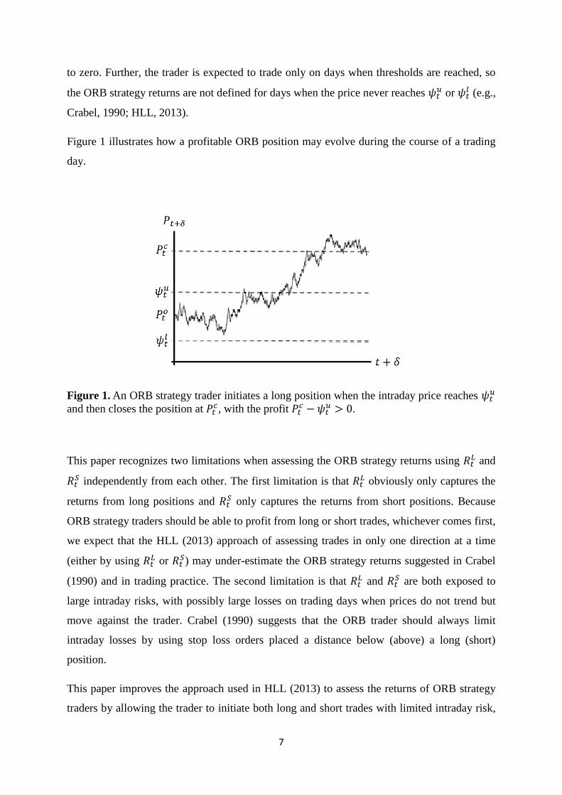
Figure 1 illustrates how a profitable ORB position may evolve during the course of a trading
day.
Figure 1. An ORB strategy trader initiates a long position when the intraday price reaches 𝜓𝑡
𝑢
and then closes the position at 𝑃𝑡𝑐, with the profit 𝑃𝑡
𝑐 − 𝜓𝑡𝑢 > 0.
This paper recognizes two limitations when assessing the ORB strategy returns using 𝑅𝑡𝐿 and
𝑅𝑡𝑆 independently from each other. The first limitation is that 𝑅𝑡
𝐿 obviously only captures the
returns from long positions and 𝑅𝑡𝑆 only captures the returns from short positions. Because
ORB strategy traders should be able to profit from long or short trades, whichever comes first,
we expect that the HLL (2013) approach of assessing trades in only one direction at a time
(either by using 𝑅𝑡𝐿 or 𝑅𝑡
𝑆) may under-estimate the ORB strategy returns suggested in Crabel
(1990) and in trading practice. The second limitation is that 𝑅𝑡𝐿 and 𝑅𝑡
𝑆 are both exposed to
large intraday risks, with possibly large losses on trading days when prices do not trend but
move against the trader. Crabel (1990) suggests that the ORB trader should always limit
intraday losses by using stop loss orders placed a distance below (above) a long (short)
position.
This paper improves the approach used in HLL (2013) to assess the returns of ORB strategy
traders by allowing the trader to initiate both long and short trades with limited intraday risk,
8
in line with Crabel (1990), still applicable to time series with daily readings of the opening,
high, low, and closing prices. We denote it the “ORB Long Strangle” returns assessment
approach because it is a futures trader’s equivalent to a Long Strangle option strategy (e.g.,
Saliba et al., 2009). The ORB Long Strangle is done in practice by placing two resting market
orders: a long position at 𝜓𝑡𝑢 and a short position at 𝜓𝑡
𝑙 , both positions remaining active
throughout the trading day. Assuming that traders can trade at continuous asset prices and to a
trading cost equal to zero, the Long Strangle produces one of three possible outcomes: 1) only
the upper threshold is crossed, yielding the return 𝑅𝑡𝐿; 2) only the lower threshold is crossed,
yielding the return 𝑅𝑡𝑆; or 3) both thresholds are crossed during the same trading day, yielding
a return equal to 𝜓𝑡𝑙 − 𝜓𝑡
𝑢 < 0. We note that, if a trader experiences an intraday double
crossing, the trader should not trade during the remainder of the trading day (e.g., Crabel,
1990). Because there are only two active orders in the Long Strangle, we can safely rule out
more than two intraday crossings. As before, ORB strategy returns are not defined for days
when the price reaches neither threshold.
This paper calculates the daily returns of the Long Strangle strategy, 𝑅𝑡𝐿&𝑆, as:
𝑅𝑡𝐿&𝑆 = {
𝑃𝑡𝑐 − 𝜓𝑡
𝑢 ⋛ 0, 𝑖𝑓 (𝑃𝑡ℎ ≥ 𝜓𝑡
𝑢) ∩ (𝑃𝑡𝑙 > 𝜓𝑡
𝑙 )
𝜓𝑡𝑙 − 𝑃𝑡
𝑐 ⋛ 0, 𝑖𝑓 (𝑃𝑡ℎ < 𝜓𝑡
𝑢) ∩ (𝑃𝑡𝑙 ≤ 𝜓𝑡
𝑙 )
𝜓𝑡𝑙 − 𝜓𝑡
𝑢 < 0, 𝑖𝑓 (𝑃𝑡ℎ ≥ 𝜓𝑡
𝑢) ∩ (𝑃𝑡𝑙 ≤ 𝜓𝑡
𝑙)
(4)
The ORB Long Strangle approach in Eq. (4) allows us to assess the returns of traders
initiating long or short positions, whichever comes first, using the opposite threshold as a stop
loss order1, effectively limiting maximum intraday losses to 𝜓𝑡
𝑙 − 𝜓𝑡𝑢 = −2𝜌 < 0 (for
symmetrically placed thresholds). Therefore, the returns 𝑅𝑡𝐿&𝑆 provide a closer approximation
of the ORB returns in Crabel (1990) relative to studying 𝑅𝑡𝐿 and 𝑅𝑡
𝑆 independently and
separately from each other. Henceforth, we refer to the ORB Long Strangle strategy as the
ORB strategy if not otherwise mentioned. This paper assumes an interest rate of money equal
to zero so that profit can only come from actively trading the ORB strategy and not from
1 One could think of other possible placements of stop loss orders but this placement is the only one tested in this
paper.
9
passive rent-seeking. In the empirical section, we also study ORB returns when trading costs
are added, and we discuss the effects on ORB returns if asset prices are not continuous.
2.3 Measuring the average daily returns across volatility states
This paper measures the average daily returns for different volatility states by grouping the
ORB returns into ten volatility states based on the deciles of the daily price returns volatility
distribution. The volatility states are ranked from low to high, with the 1: 𝑠𝑡 decile as the state
with the lowest volatility and the 10: 𝑡ℎ decile as the state with the highest volatility.
We then calculate the average daily return for each volatility state by the following dummy
variable regression, given 𝜌:
𝑅𝜌,𝑡𝐿&𝑆 = ∑ 𝑎𝜌,𝜏𝐷𝜌,𝜏
10
𝜏=1
+ 𝑣𝜌,𝑡 (5)
where 𝑎𝜌,𝜏 is the average ORB return in the 𝜏: 𝑡ℎ volatility state, 𝐷𝜌,𝜏 is a binary variable
equal to one if the returns corresponds to the 𝜏: 𝑡ℎ decile of the volatility distribution, or zero
otherwise, and 𝑣𝜌,𝑡 is the error term. From the expected (positive) correlation between ORB
returns and volatility, the ORB returns will experience heteroscedasticity and possibly serial
correlation. To assess the statistical significance of Regression (5), we therefore apply
Ordinary Least Squares (OLS) estimation using Newey-West Heteroscedasticity and
Autocorrelated Consistent (HAC) standard errors.
The 𝐷𝜌,𝜏 in Regression (5) requires that we estimate the volatility. Unfortunately, volatility,
𝜎𝑡+𝛿, is not directly observable (e.g., Andersen and Bollerslev, 1998). Another challenge for
this study is to estimate intraday volatility over the time interval 0 ≤ 𝛿 ≤ 1, when limited to
time series with daily readings of the opening, high, low, and closing prices.
Making good use of the data at hand, this paper uses the simplest available approach to
estimate daily volatility 𝜎𝑡+1 by tracking the daily absolute return (log-difference of prices) of
day 𝑡:
10
𝜎𝑡𝑐 = +√(𝑃𝑡
𝑐 − 𝑃𝑡𝑜)2 = |𝑃𝑡
𝑐 − 𝑃𝑡𝑜| (6)
Using absolute returns as a proxy for volatility is the basis of much of the modeling effort
presented in the volatility literature (e.g., Taylor, 1987; Andersen and Bollerslev, 1998;
Granger and Sin, 2000; Martens et al., 2009), and has shown itself to be a better measurement
of volatility than squared returns (Forsberg and Ghysels, 2007). Although 𝜎𝑡𝑐 is unbiased, i.e.,
𝐸𝑡𝜎𝑡𝑐 = 𝜎𝑡+1, it is a noisy estimator (e.g., Andersen and Bollerslev, 1998). One extreme
example would be a very volatile day, with widely fluctuating prices, but where the closing
price is the same as the opening price. The daily open-to-close absolute return would then be
equal to zero, whereas the actual volatility has been non-zero. Because positive ORB returns
imply a closing price at a relatively large (absolute) distance from the opening price, we
expect reduction in noise for the higher levels of positive ORB returns.
Because the ORB strategy trader is profiting from intraday price trends, it stands to reason
that he should increase his return on days when volatility is relatively high. When using 𝜎𝑡𝑐 to
estimate volatility, the relationship between intraday momentum (by Eq. (3)) and volatility is
straightforward. For a profitable long trade, we have the relationship 𝑅𝑡𝐿&𝑆 = 𝑃𝑡
𝑐 − 𝜓𝑡𝑢 =
𝑃𝑡𝑐 − 𝑃𝑡
𝑜 − 𝜌 = 𝜎𝑡𝑐 − 𝜌 because 𝑅𝑡
𝐿&𝑆 = 𝑃𝑡𝑐 − 𝜓𝑡
𝑢 > 0 and 𝑃𝑡𝑐 − 𝑃𝑡
𝑜 = 𝜎𝑡𝑐 > 0. For a
profitable short trade, we have the relationship 𝑅𝑡𝐿&𝑆 = −(𝑃𝑡
𝑐 − 𝜓𝑡𝑙) = −(𝑃𝑡
𝑐 − 𝑃𝑡𝑜 + 𝜌) =
−(−𝜎𝑡𝑐 + 𝜌) = 𝜎𝑡
𝑐 − 𝜌 because 𝑅𝑡𝐿&𝑆 = −(𝑃𝑡
𝑐 − 𝜓𝑡𝑙) > 0 and 𝑃𝑡
𝑐 − 𝑃𝑡𝑜 = −𝜎𝑡
𝑐 < 0. Thus, a
positive ORB return equals the volatility minus the range for both long and short trades.
From this exercise, we learn that the ORB strategy trader should increase his expected return
during days of relatively high volatility and decrease his expected return during days of
relatively low volatility, suggesting different expected returns in different volatility states. In
addition, we learn that positive ORB returns imply high volatility, but not the other way
around, since the ORB strategy trader still can experience losses when volatility is high,
associated with intraday double crossing: 𝑅𝑡𝐿&𝑆 = 𝜓𝑡
𝑙 − 𝜓𝑡𝑢 = −2𝜌 < 0.
When a price series is given in a daily open, high, low, and close format, Taylor (1987)
proposes that the (log) price range in day 𝑡 (𝜍𝑡 = 𝑃𝑡ℎ − 𝑃𝑡
𝑙 > 0) could also serve as a suitable
measure of the daily volatility. To strengthen the empirical results, this paper also estimates
11
daily volatility 𝜎𝑡+1 by the price range of day 𝑡, i.e., 𝜍𝑡. Finding qualitatively identical results
whether we use 𝜍𝑡 or 𝜎𝑡𝑐, we report only the empirical results when using 𝜎𝑡
𝑐.
3. Empirical results
3.1 Data
We apply the ORB strategy to long time series of crude oil futures and of S&P 500 futures.
Futures contracts are used in this paper because long time series are readily available, and
because futures are the preferred investment vehicle when trading the ORB strategy in
practice (e.g., Crabel, 1990; Williams, 1999; Fisher, 2002). There are many reasons why
futures are the preferable investment vehicle relative to, for example, stocks. Futures are as
easily sold short as bought long, are not subject to short-selling restrictions, and can be bought
on a margin, providing attractive leverage possibilities for day traders who wish to increase
profit. In addition, costs associated with trading, such as commissions and bid-ask spreads, are
typically smaller in futures contracts than in stocks due to the relatively high liquidity.
The data includes daily readings of the opening, high, low, and closing prices, during the US
market opening hours. We note that ORB traders should trade only during the US market
opening hours, when the liquidity is high, even if futures contracts may trade for 24 hours
(Crabel, 1990). Thus, the US market opening period is the only time interval of interest for the
study of this paper.
The crude oil price series covers the period January 2, 1991 to January 26, 2011 and the S&P
500 price series covers the period January 2, 1991 to November 29, 2010. Both series are
obtained from Commodity Systems Inc. (CSI) and are adjusted for roll-over effects such as
contango and backwardation by CSI. The future contract typically rolls out on the 20th
of each
month, one month prior to the expiration month; see Pelletier (1997) for technical details. We
analyze the series separately and independent of each other.
Figures 2 and 3 illustrate the price series over time for crude oil and S&P 500 futures,
respectively.
12
Figure 2. The daily closing prices for crude oil futures over time, adjusted for roll-over
effects, from January 2, 1991 to January 26, 2011. Source: Commodity Systems Inc.
Figure 3. The daily closing prices for S&P 500 futures over time, adjusted for roll-over
effects, from January 2, 1991 to November 29, 2010. Source: Commodity Systems Inc.
40
60
80
100
120
140
160
180
200
19910102 19951010 20000726 20050519 20100702
Clo
sin
g p
rice
cru
de
oil
600
800
1000
1200
1400
1600
1800
19910102 19950929 20000630 20050413 20100119
Clo
sin
g p
rice
S&
P5
00
13
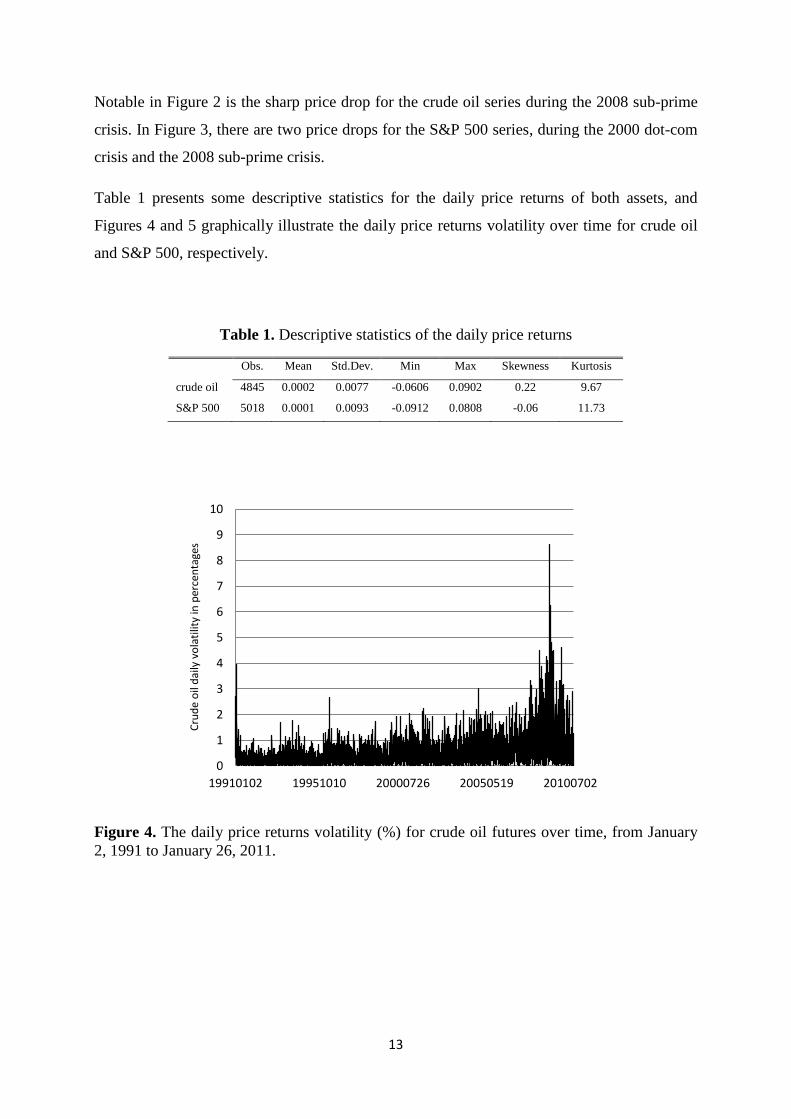
Notable in Figure 2 is the sharp price drop for the crude oil series during the 2008 sub-prime
crisis. In Figure 3, there are two price drops for the S&P 500 series, during the 2000 dot-com
crisis and the 2008 sub-prime crisis.
Table 1 presents some descriptive statistics for the daily price returns of both assets, and
Figures 4 and 5 graphically illustrate the daily price returns volatility over time for crude oil
and S&P 500, respectively.
Table 1. Descriptive statistics of the daily price returns
Obs. Mean Std.Dev. Min Max Skewness Kurtosis
crude oil 4845 0.0002 0.0077 -0.0606 0.0902 0.22 9.67
S&P 500 5018 0.0001 0.0093 -0.0912 0.0808 -0.06 11.73
Figure 4. The daily price returns volatility (%) for crude oil futures over time, from January
2, 1991 to January 26, 2011.
0
1
2
3
4
5
6
7
8
9
10
19910102 19951010 20000726 20050519 20100702
Cru
de
oil
dai
ly v
ola
tilit
y in
per
cen
tage
s
14
Figure 5. The daily price returns volatility (%) for S&P 500 futures over time, from January
2, 1991 to November 29, 2010.
Table 1 shows that daily price returns display the expected characteristics of empirical returns
series, with close-to-zero means and positive kurtosis for both assets. As expected, we can
confirm that the means for crude oil and S&P 500 are not significantly larger than zero,
although this is not explicitly shown. Figures 4 and 5 reveal apparent volatility clustering over
time for both assets. These results are expected for empirical returns (e.g., Cont 2001).
3.2 The average daily returns across volatility states
This paper assesses strategy returns for different levels of 𝜌, ranging from small to large,
thereby spanning the profit opportunities of ORB strategies. For simplicity and without loss
of information, we only present the results for thresholds 𝜌𝜖{0.5%, 1.0%, 1.5%, 2.0%}, for
both assets. Figures 6-9 and Figures 10-13 present the average daily ORB returns across
volatility states for crude oil futures and for S&P 500 futures, respectively. We illustrate the
ORB returns in basis points (%%), (𝑎 ∙ 10 000), where 𝑎 is the average ORB return for a
given volatility state (see the definition of 𝑎 in the previous section). We use 95% point-wise
confidence intervals based on the HAC standard errors.
0
1
2
3
4
5
6
7
8
9
10
19910102 19950929 20000630 20050413 20100119
S&P
50
0 d
aily
vo
lati
lity
in p
erce
nta
ges
15
Figure 6. Average returns (bp:s) across
volatility states (𝜏) when trading crude oil
futures using 𝜌 = 0.5%. We use 95%
confidence intervals based on the HAC
standard errors.
Figure 7. Average returns (bp:s) across
volatility states (𝜏) when trading crude oil
futures using 𝜌 = 1.0%. We use 95%
confidence intervals based on the HAC
standard errors.
Figure 8. Average returns (bp:s) across
volatility states (𝜏) when trading crude oil
futures using 𝜌 = 1.5%. We use 95%
confidence intervals based on the HAC
standard errors.
Figure 9. Average returns (bp:s) across
volatility states (𝜏) when trading crude oil
futures using 𝜌 = 2.0%. We use 95%
confidence intervals based on the HAC
standard errors.
-100
-50
0
50
100
150
200
10th 40th 70th 100th
OR
B R
etu
rns
in b
asis
po
ints
Percentile of daily volatility
upper confidence levelparameterlower confidence level
-100
-50
0
50
100
150
200
250
10th 40th 70th 100th
OR
B R
etu
rns
in b
asis
po
ints
Percentile of daily volatility
upper confidence levelparameterlower confidence level
-200
-100
0
100
200
300
10th 40th 70th 100th
OR
B R
etu
rns
in b
asis
po
ints
Percentile of daily volatility
upper confidence levelparameterlower confidence level
-200
-100
0
100
200
300
10th 40th 70th 100th
OR
B R
etu
rns
in b
asis
po
ints
Percentile of daily volatility
upper confidence levelparameterlower confidence level
16
Figure 10. Average returns (bp:s) across
volatility states (𝜏) when trading S&P 500
futures using 𝜌 = 0.5%. We use 95%
confidence intervals based on the HAC
standard errors.
Figure 11. Average returns (bp:s) across
volatility states (𝜏) when trading S&P 500
futures using 𝜌 = 1.0%. We use 95%
confidence intervals based on the HAC
standard errors.
Figure 12. Average returns (bp:s) across
volatility states (𝜏) when trading S&P 500
futures using 𝜌 = 1.5%. We use 95%
confidence intervals based on the HAC
standard errors.
Figure 13. Average returns (bp:s) across
volatility states (𝜏) when trading S&P 500
futures using 𝜌 = 2.0%. We use 95%
confidence intervals based on the HAC
standard errors.
Figures 6-13 show significantly negative returns for lower volatility states, 𝜏 ≤ 3, and
significantly positive returns for higher volatility states, 𝜏 ≥ 7, for both assets. That is, the
average daily returns from day trading using ORB strategies are correlated with volatility. The
difference in average daily returns between state 1 and 10 are remarkably high – around 200
basis points per day for crude oil and around 150 basis points per day for S&P 500, given
𝜌 = 0.5%. For larger 𝜌: 𝑠, the differences grow even larger.
Because the returns are calculated daily, relatively small differences in the average daily
returns have substantial effects on wealth when annualized. The annualized return from a 200
-100
-50
0
50
100
150
10th 40th 70th 100th
OR
B R
etu
rns
in b
asis
po
ints
Percentile of daily volatility
upper confidence levelparameterlower confidence level
-150
-100
-50
0
50
100
150
200
250
10th 40th 70th 100th
OR
B R
etu
rns
in b
asis
po
ints
Percentile of daily volatility
upper confidence levelparameterlower confidence level
-150
-50
50
150
250
350
10th 40th 70th 100th
OR
B R
etu
rns
in b
asis
po
ints
Percentile of daily volatility
upper confidence levelparameterlower confidence level
-200
-100
0
100
200
300
400
10th 40th 70th 100th
OR
B R
etu
rns
in b
asis
po
ints
Percentile of daily volatility
upper confidence levelparameterlower confidence level
17
point daily difference between state 1 and state 10 amounts to (1 + 0.02)240 − 1 = 115 %,
and a 150 point daily difference amounts to (1 + 0.015)240 − 1 = 35 %, given 240 trading
days in a year. Thus, the annualized returns differ substantially for a day trader consistently
trading in the lowest volatility state compared to one trading in the highest volatility state.
This is merely an example to illustrate the effect that daily returns have on annualized returns;
however, it should not be taken as the result of actual trading. This is because the results so
far are based on the assumption that the trader a priori knows the volatility state; in this
respect, these are in-sample results. In actual trading, traders do not a priori know the
volatility state and are not able to trade assets in high volatility states every day.
To shed more light on profitability when using the ORB strategy in actual trading, this paper
also assesses the ORB strategy returns without a priori knowledge of the volatility state
among traders, i.e., the results of trading out-of-sample. We assess both daily and annual
returns because both are relevant for traders – a strategy yielding a high daily return on
average is of limited use to a trader who trades only once a year.
3.3 Returns when trading the ORB strategy out-of-sample
When trading the ORB strategy, the idea is to restrict trading only to expansion days (high
volatility) and avoid trading during contraction days (normal or low volatility). When trading
out-of-sample, however, the trader does not a priori know the volatility state, so some form of
volatility prediction is necessary. The trader either can try to predict volatility states using
econometric approaches (e.g., Engle, 1982; Andersen and Bollerslev, 1998) or can use the
ORB strategy approach (Crabel, 1990; Williams, 1999; Fisher, 2002), identifying the range as
a volatility predictor by itself and setting the range large enough so that only large volatility
days are able to reach the thresholds.
This paper assesses the average daily returns when trading the ORB strategy out-of-sample,2
following the approach of Crabel (1990), Williams (1999), and Fisher (2002), i.e., setting the
range large enough so that only large volatility days are able to reach the thresholds. We
estimate the average daily returns with the regression 𝑅𝜌,𝑡𝐿&𝑆 = 𝐴𝜌 + 𝜔𝜌,𝑡, where 𝐴𝜌 is the
2 We tried various ARCH and GARCH specifications to predict the volatility state, but without improving the
results in any significant way. We find that expansion days, which result in high ORB returns, tend to come
unexpectedly after a number of contraction days. Further, expansion days do not typically appear two days in a
row. Thus, the volatility prediction models do not have time to react. This is perhaps the reason why the ARCH
and GARCH specifications are unable to improve the trading results.
18
average daily return of the ORB strategy during days with predicted high volatility, and 𝜔𝑡 is
the error term, given a certain range.
The results for both assets are given in Table 2:
Table 2. Daily returns when trading the ORB strategy out-of-sample. 𝜌 is the per cent
distance added to and subtracted from the opening price. 𝑇 is the number of trades. 𝑓𝑟𝑒𝑞
gives the proportion of trades that result in positive returns, while 𝐴 gives the average daily
return. The p-values are calculated based on the HAC standard errors. No trading costs are
included.
𝜌(%) T freq. 𝐴 𝑝
0.5 2827 0.57 0.0013 0.0000
crude oil 1.0 1044 0.58 0.0020 0.0000
1.5 423 0.61 0.0027 0.0000
2.0 189 0.67 0.0036 0.0001
𝜌(%) T freq. 𝐴 𝑝
0.5 3314 0.49 0.0004 0.0057
S&P 500 1.0 1572 0.53 0.0006 0.0267
1.5 749 0.52 0.0006 0.1755
2.0 368 0.52 0.0006 0.4937
Table 2 shows mixed results when trading the ORB strategy out-of-sample. We find
significantly positive returns for all ranges at the 95% confidence level when trading crude oil
futures out-of-sample, and it seems that returns increase with 𝜌. When trading S&P 500
futures out-of-sample, however, we find significantly positive returns only for the two smaller
ranges, 𝜌 = 0.5 and 𝜌 = 1.0, at the 95% confidence level. For ranges larger than 𝜌 = 1.0,
e.g., 𝜌 = 1.5 and 𝜌 = 2.0, we cannot reject the null hypothesis of zero returns on average.
When separating the (Long Strangle) returns between long and short trades when trading S&P
500, we find that the average returns of short trades, initially positive, are reduced for
𝜌 > 1.0% while the returns of long trades seem to increase with 𝜌, as in the crude oil
example. This difference in average returns between long and short ORB trades drives the
results although this is not explicitly shown. Regardless of the reasons why, it is clear that not
all ranges are profitable when trading the S&P 500 out-of-sample. Thus, profitability when
trading the ORB strategy out-of-sample depends on the choice of asset and range. Using the
“wrong” range for a particular asset, for example, using 𝜌 = 1.5 or 𝜌 = 2.0 when trading
19
S&P 500, the ORB strategy does not necessarily yield a daily return significantly larger than
zero on average.
To compare these returns with the returns of an alternative investment strategy, we also study
the difference between the return of the ORB strategy (𝑅𝑡𝐿&𝑆) for day 𝑡 and the corresponding
return of the so-called buy and hold strategy (𝑅𝑡𝐵&𝐻 = 𝑃𝑡
𝑐 − 𝑃𝑡−1𝑐 ). The buy and hold strategy
is a straightforward strategy where the trader buys the asset and holds it until the expiration of
the future contract, at which point the position is “rolled over” onto the next contract. As it
turns out, the buy and hold strategy returns are close to zero; when running the regression
𝑅𝑡𝐿&𝑆 − 𝑅𝑡
𝐵&𝐻 = �̃� + �̃�𝑡, we find qualitatively the same results as illustrated in Table 2, for
both assets, although not explicitly shown. That is, when trading crude oil futures out-of-
sample, we find empirical support that the ORB strategy yields a larger average daily return
for all ranges compared to the buy and hold strategy. When trading S&P 500 futures out-of-
sample, on the other hand, we find empirical support that the ORB strategy yields a larger
average daily return only for 𝜌 = 0.5 and 𝜌 = 1.0, compared to the buy and hold strategy.
We now investigate what a day trader can expect in terms of accumulated annual returns
when trading the ORB strategy out-of-sample. We start by plotting the wealth accumulation
over time starting at 1991-01-01 with a value of 1 000 000 USD, for all ranges, and for both
assets. Profit is reinvested on to the next trade. The wealth accumulation of the buy and hold
(B&H) strategy is included as a reference. Figures 14-15 plot the wealth accumulation over
time when applying the B&H and the ORB strategy to trade crude oil futures and S&P 500
futures, respectively, out-of-sample. Table 3 presents the corresponding out-of-sample annual
returns statistics (calendar year).
20
Figure 14. Wealth over time, starting with 1 000 000 USD (expressed in log levels), when
trading crude oil futures out-of-sample using ORB strategies for all ranges from January 1,
1991 to January 26, 2011. B&H refers to the buy and hold strategy, and ORB refers to the
ORB strategy given a particular range. No trading costs are included.
Figure 15. Wealth over time, starting with 1 000 000 USD (expressed in log levels), when
trading S&P 500 futures out-of-sample using ORB strategies for all ranges from January 1,
1991 to November 29, 2010. B&H refers to the buy and hold strategy, and ORB refers to the
ORB strategy for a particular range. No trading costs are included.
13
14
15
16
17
18
19910101 19951009 20000725 20050518 20100701
Wea
lth
ove
r ti
me
(lo
g le
vels
)
B&H
ORB 0.5
ORB 1.0
ORB 1.5
ORB 2.0
13
14
15
19910101 19950928 20000629 20050412 20100115
Wea
lth
ove
r ti
me
(lo
g le
vels
)
B&H
ORB 0.5
ORB 1.0
ORB 1.5
ORB 2.0
21
Table 3. Annual returns (calendar year) when trading the B&H strategy and the ORB strategy
out-of-sample. 𝜌 is the per cent distance added to and subtracted from the opening price,
where N/A refers to the B&H strategy. Mean/Std.Dev gives the average annual return per unit
of annual volatility and Mean/-Min gives the average annual return over the largest annual
loss. No trading costs are included.
𝜌(%) Obs. Mean Std.Dev. Min Max Mean/Std.Dev. Mean/-Min
N/A 19 0.0530 0.1672 -0.2505 0.3864 0.32 0.21
0.5 19 0.3055 0.7110 -0.0493 2.5527 0.43 6.19
crude oil 1.0 19 0.1568 0.4244 -0.0758 1.3994 0.37 2.07
1.5 19 0.0725 0.2180 -0.0214 0.7740 0.33 3.39
2.0 19 0.0391 0.1179 -0.0189 0.3866 0.33 2.07
𝜌(%) Obs. Mean Std.Dev Min Max Mean/Std.Dev Mean/-Min
N/A 19 0.0250 0.1061 -0.1791 0.2665 0.24 0.14
0.5 19 0.0661 0.1655 -0.0784 0.6995 0.40 0.84
S&P 500 1.0 19 0.0562 0.1876 -0.1222 0.7946 0.30 0.46
1.5 19 0.0243 0.0848 -0.0557 0.3673 0.29 0.44
2.0 19 0.0087 0.0253 -0.0208 0.0720 0.34 0.42
Figures 14-15 illustrate that wealth accumulates unevenly over time and primarily during time
periods connected to market crisis events with high volatility, for both assets. Even when
ORB traders profit in the long run, we observe long periods of negative growth in wealth for
both assets. Hence, profitability is not robust to time. Moreover, Figures 14-15 graphically
show that long-run profit using ORB strategies is the result of relatively infrequent trades of a
relatively large magnitude, associated with the infrequent time periods of market crisis, i.e.,
periods of high volatility.
Table 3 shows that the optimal levels of the range for maximizing annual returns are the
relatively small range, 𝜌 = 0.5%, for both assets. Table 3 illustrates further that traders using
the B&H strategy can achieve larger annual returns on average (Mean) than traders using
ORB strategies for some ranges (𝜌 = 2.0% for crude oil, and 𝜌 = 1.5% and 𝜌 = 2.0% for
S&P 500). One reason for the relatively low annual returns when trading ORB strategies is
the relatively low frequency of trading (especially when using large ranges). As we increase
the range, we remember from Table 2 that the number of trades (𝑇) decreases. Fewer trades,
in turn, decreases annual returns, ceteris paribus. We note that low annual returns due to few
trades can, to some extent, be offset by trading many assets simultaneously, but this is not
studied in this paper.
22
Table 3 further shows that ORB strategies yield larger risk-adjusted returns (measured by
Mean/Std.Dev and Mean/-Min) than the buy and hold strategy, for all ranges and for both
assets. This is interesting from a risk-return point of view because risk-averse day traders
could benefit from using ORB strategies compared to the buy and hold strategy. ORB
strategies seem especially attractive in terms of high Mean/-Min due to relatively moderate
largest annual losses (min).
3.3.1 Sensitivity analysis regarding price jumps
Prices are not always continuous within a trading day but may experience so-called price
jumps in the direction of the most recent price movement (e.g., Mandelbrot, 1963; Fama and
Blume, 1966). Because of the price jumps, the trader may experience an order fill at worse
prices than expected. Consequently, we may over-estimate the actual return from trading if
the effects of price jumps are not taken into account when assessing the returns of technical
trading strategies based on intraday thresholds (see, for example, the technical trading strategy
in Alexander, 1961). This paper recognizes that possible price jumps will affect the returns of
trading, but not necessarily in a negative way when we consider the ORB strategy.
This paper estimates the effects of price jumps on ORB returns in two stages of the trade.
First, we model the price jump effect in market entries and, second, in market exits. First,
because price jumps occur in the direction of the most recent price movement, the ORB
traders’ entry prices are sometimes filled at some other price than the threshold. If �̃�𝑡 denotes
the actual entry price on day 𝑡, we may write the price jump effects for long trades as
�̃�𝑡𝑢 > 𝜓𝑡
𝑢, and for short trades as �̃�𝑡𝑙 < 𝜓𝑡
𝑙 , where the actual trading price is based on the
range plus a price jump, �̃� = 𝜌 + 휀, where 휀 > 0 is the size of the price jump. We consider
here a reasonable estimate of 휀 = 2 basis points when trading crude oil and S&P 500 futures
(based on empirical observations when trading futures with the ORB strategy using an
account size of around 1 000 000 USD, Interactive Brokers, www.interactivebrokers.com,
February 2, 2010 to November 29, 2010).
Second, because ORB traders exit the market at the market close, there cannot be a jump to
some other level. Thus, 𝑃𝑡𝑐 is the actual closing price of day 𝑡. Moreover, in contrast to the
technical trading strategy of Alexander (1961), where both market entry and exit are based on
intraday threshold crossing, the ORB strategy is only affected by possible price jumps at the
23
market entry level. From Figures 6-13 and Table 2, we observe that the effect of price jumps
of 휀 = 2 basis points on returns is not necessarily negative when trading the ORB strategy. In
fact, we find that the price jump effect on the average returns is positive for larger 𝜌 when
trading crude oil, and either negative or positive, depending on the initial level of 𝜌, when
trading S&P 500.
From this reasoning, we do not expect price jumps to qualitatively change the results shown
in Figures 6-13 and Table 2, i.e., returns significantly larger (smaller) than zero will most
likely remain significantly larger (smaller) than zero.
3.3.2 Sensitivity analysis regarding trading costs
Trading costs in terms of commission fees and bid-ask spreads will consume some of the
profits. For the assets under consideration, these costs are relatively small during the trading
hours of the US markets. We estimate that we need to subtract 4 basis points per trade, or 8
basis points roundtrip daily cost, for crude oil futures. For the S&P 500, we need to subtract
1.5 basis points per trade, or 3 basis points roundtrip daily cost (based on empirical
observations when trading futures with the ORB strategy, using an account size of around
1 000 000; USD Interactive Brokers, www.interactivebrokers.com, February 2, 2010 to
November 29, 2010).
We recognize that these levels of trading costs are not large enough to qualitatively change
the results for the average daily returns shown in Figures 6-13 or in Table 2; that is, returns
significantly (insignificantly) larger than zero will remain significantly (insignificantly) larger
than zero even if trading costs are included. We find, however, that even small levels of
trading costs have a large effect on the accumulation of wealth over time and on the
corresponding annual returns, when trading ORB strategies out-of-sample.
Figures 16-17 graphically show the accumulation of wealth over time when trading ORB
strategies out-of-sample, adjusted for trading costs, applied to crude oil and S&P 500,
respectively. Table 4 gives the corresponding annual returns statistics for both assets.
24
Figure 16. Wealth over time, starting with 1 000 000 USD (expressed in log levels), when
trading crude oil futures out-of-sample, with trading costs included, from January 1, 1991 to
January 26, 2011. B&H refers to the buy and hold strategy, and ORB refers to the ORB
strategy given a particular range. We subtract 8 basis points roundtrip daily cost during
trading days for ORB strategies, and a roundtrip daily cost of 8/20 basis points for the B&H
strategy (we assume that contracts are rolled each month and that each month consists of 20
trading days).
Figure 17. Wealth over time, starting with 1 000 000 USD (expressed in log levels), when
trading S&P 500 futures out-of-sample, with trading costs included, from January 1, 1991 to
November 29, 2010. B&H refers to the buy and hold strategy, and ORB refers to the ORB
strategy for a particular range. We subtract 3 basis points roundtrip daily cost during trading
days for ORB strategies, and a roundtrip daily cost of 3/20 basis points for the B&H strategy
(we assume that contracts are rolled each month and that each month consists of 20 trading
days).
12
13
14
15
16
17
18
19910101 19951009 20000725 20050518 20100701
Wea
lth
ove
r ti
me
(lo
g le
vels
)
B&H
ORB 0.5
ORB 1.0
ORB 1.5
ORB 2.0
13
14
15
19910101 19950928 20000629 20050412 20100115
Wea
lth
ove
r ti
me
(lo
g le
vels
)
B&H
ORB 0.5
ORB 1.0
ORB 1.5
ORB 2.0
25
Table 4. Annual returns statistics (calendar year) when trading the B&H strategy and the
ORB strategy out-of-sample when trading costs are included. 𝜌 is the per cent distance added
to and subtracted from the opening price, where N/A refers to the B&H strategy.
Mean/Std.Dev gives the average annual return per unit of annual volatility and Mean/-Min
gives the average annual return over the largest annual loss. When trading crude oil futures,
we subtract 8 basis points roundtrip daily cost during trading days for ORB strategies, and a
roundtrip daily cost of 8/20 basis points for the B&H strategy. When trading S&P 500 futures,
we subtract 3 basis points roundtrip daily cost during trading days for ORB strategies, and a
roundtrip daily cost of 3/20 basis points for the B&H strategy (we assume that contracts are
rolled each month and that each month consists of 20 trading days).
𝜌(%) Obs. Mean Std.Dev. Min Max Mean/Std.Dev. Mean/-Min
N/A 19 0.0429 0.1658 -0.2580 0.3739 0.26 0.17
0.5 19 0.1568 0.5930 -0.2016 2.0990 0.26 0.78
crude oil 1.0 19 0.0993 0.3490 -0.1128 1.1638 0.28 0.88
1.5 19 0.0505 0.1798 -0.0718 0.6123 0.28 0.70
2.0 19 0.0298 0.0980 -0.0221 0.3315 0.30 1.35
𝜌(%) Obs. Mean Std.Dev Min Max Mean/Std.Dev Mean/-Min
N/A 19 0.0212 0.1057 -0.1822 0.2617 0.20 0.12
0.5 19 0.0135 0.1482 -0.1416 0.5779 0.09 0.10
S&P 500 1.0 19 0.0300 0.1687 -0.1528 0.6954 0.18 0.20
1.5 19 0.0123 0.0738 -0.0670 0.3120 0.17 0.18
2.0 19 0.0031 0.0239 -0.0212 0.0681 0.13 0.15
Figures 16-17 graphically show considerably reduced wealth levels for both assets when
trading costs are included, compared to the wealth levels in Figures 14-15. When trading
crude oil, terminal wealth is reduced 49% (𝜌 = 0.5%), 37% (𝜌 = 1.0%), 30% (𝜌 = 1.5%),
and 24% (𝜌 = 2.0%). When trading S&P 500, terminal wealth is reduced 80% (𝜌 = 0.5%),
47% (𝜌 = 1.0%), 49% (𝜌 = 1.5%), and 64% (𝜌 = 2.0%). For the buy and hold strategy,
wealth is reduced 19% and 15%, for crude oil and S&P 500, respectively.
Table 4 shows that annual returns and risk-adjusted returns decrease considerably for both
assets when trading costs are included. Further, we find that the optimal range for maximizing
annual returns remains at 𝜌 = 0.5% for crude oil but increases to 𝜌 = 1.0% for S&P 500 due
to the increase in trading costs. In sum, trading costs decrease wealth accumulation and
annual returns considerably but do not affect average daily returns shown in Table 2 in a
qualitative way.
26
4. Concluding discussion
This paper assesses the returns of the Opening Range Breakout (ORB) strategy across
volatility states. We calculate the average daily returns of the ORB strategy for each volatility
state of the underlying asset when applied on long time series of crude oil and S&P 500
futures contracts. This paper contributes to the literature on day trading profitability by
studying the returns of a day trading strategy for different volatility states. As a minor
contribution, this paper improves the HLL (2013) approach of assessing ORB strategy returns
by allowing the ORB trader to trade both long and short positions and to use stop loss orders,
in line with the original ORB strategy in Crabel (1990) and in trading practice.
When empirically tested on long time series of crude oil and S&P 500 futures contracts, this
paper finds that the average ORB return increases with the volatility of the underlying asset.
Our results relate to the findings in Gencay (1998), in that technical trading strategies tend to
result in higher profits when markets “trend” or in times of high volatility. This paper finds
that the differences in average returns between the highest and lowest volatility state are
around 200 basis points per day for crude oil, and around 150 basis points per day for S&P
500. This finding explains the significantly positive ORB returns in the period 2001-10-12 to
2011-01-26 found in HLL (2013) but also, perhaps more importantly, relates to the way we
view profitable day traders. When reading the trading literature (e.g., Crabel, 1990; Williams,
1999; Fisher, 2002) and the account studies literature (e.g., Coval et al., 2005; Barber et al.,
2011; Kuo and Lin, 2013), one may get the impression that long-run profitability in day
trading is the same as earning steady profit over time. The findings of this paper suggest
instead that long-run profitability in day trading is the result of trades that are relatively
infrequent but of relatively large magnitude and are associated with the infrequent time
periods of high volatility. Positive returns in day trading can hence be seen as a tail event
during periods of high volatility of an otherwise efficient market. The implication is that a day
trader, profitable in the long run, could still experience time periods of zero, or even negative,
average returns during periods of normal, or low, volatility. Thus, even if long-run
profitability in day trading could be achieved, it is achieved only by the trader committed to
trade every day for a very long period of time or by the opportunistic trader able to restrict his
trading to periods of high volatility. Further, this finding highlights the need for using a
relatively long time series that contains a wide range of volatility states when evaluating the
returns of day traders, in order to avoid possible volatility bias.
27
With trading ORB strategies out-of-sample, we find that profitability depends on the choice of
asset and range, and that not all ranges are profitable. We find that the ORB strategy is
profitable for all ranges when trading crude oil, but, when trading the S&P 500, the ORB
strategy does not necessarily yield a daily return significantly larger than zero on average for
some of the ranges. Further, we find that profitability is not robust to time. Even when ORB
strategies are profitable in the long run, ORB strategies still lose money during periods of
time when volatility is normal or low. If the trader, for example, is unfortunate enough to start
trading the ORB strategy after a market crisis event, when the volatility has moved back to a
low volatility state, it could take a long time, sometimes years, of day trading until the trader
starts to profit. We believe this finding to be worrisome news for a trader looking to day
trading as an alternative source of regular income instead of employment. A point to note is
that ORB strategies result in relatively few trades, which restricts potential wealth
accumulation over time. Most likely, the ORB trader simultaneously monitors and trades on
several different markets, thereby increasing the frequency of trading. Further, this paper
studies profitability when trading the ORB strategy without leverage (leverage means that the
trader could have a market exposure larger than the value of trading capital), which also may
restrict potential wealth accumulation over time. Most likely, the ORB trader uses leverage to
increase the returns from trading. Moreover, we find that trading costs do not affect average
daily returns in a qualitative way but decrease annual returns considerably.
For future research, it would be of interest to study whether the returns of other strategies used
by day traders also correlate with volatility. In addition, it would be of interest to study
whether the returns of momentum-based strategies with longer investment periods than
intraday (see, for example, the strategies in Jegadeesh and Titman, 1993; Erb and Harvey,
2006; Miffre and Rallis, 2007) correlate with volatility.
28
References
Alexander, S. (1961): “Price Movements in Speculative Markets: Trends or Random Walks,”
Industrial Management Review, 2, 7-26.
Andersen, T.G., and T. Bollerslev (1998): “Answering the skeptics: Yes, standard volatility
models do provide accurate forecasts,” International Economic Review, 39, 885-905.
Barber, B.M., Y. Lee, Y. Liu, and T. Odean (2006): “Do Individual Day Traders Make
Money? Evidence from Taiwan,” Working Paper. University of California at Davis and
Peking University and University of California, Berkeley.
Barber, B.M., Y. Lee, Y. Liu, and T. Odean (2011): “The cross-section of speculator skill:
Evidence from day trading,” Working Paper. University of California at Davis and Peking
University and University of California, Berkeley.
Barber, B.M., and T. Odean (1999): “The Courage of Misguided Convictions.” Financial
Analysts Journal, 55, 41-55.
Barberis, N., A. Shleifer, and R. Vishny (1998): “A Model of Investor Sentiment," Journal of
Financial Economics, 49, 307-343.
Cont, R. (2001): “Empirical properties of asset returns: stylized facts and statistical issues.”
Quantitative Finance, 1, 223-236.
Coval, J.D., D.A. Hirshleifer, and T. Shumway (2005): “Can Individual Investors Beat the
Market?” Working Paper No. 04-025. School of Finance, Harvard University.
Crabel, T. (1990): Day Trading With Short Term Price Patterns and Opening Range
Breakout, Greenville, S.C.: Traders Press.
29
Crombez, J. (2001): “Momentum, Rational Agents and Efficient Markets," Journal of
Psychology and Financial Markets, 2, 190-200.
Daniel, K., D. Hirshleifer, and A. Subrahmanyam (1998): “Investor Psychology and Security
Market Under- and Overreactions" Journal of Finance, 53, 1839-1885.
Engle, R. F. (1982): “Autoregressive Conditional Heteroscedasticity with Estimates of the
Variance of United Kingdom Inflation," Econometrica, 50.
Fama, E. (1965): “The Behavior of Stock Market Prices," Journal of Business, 38, 34-105.
Fama, E. (1970): “Efficient Capital Markets: A Review of Theory and Empirical Work," The
Journal of Finance, 25, 383-417.
Fama, E. and M. Blume (1966): “Filter Rules and Stock Market Trading Profits," Journal of
Business, 39, 226-241.
Fisher, M. (2002): The Logical Trader: Applying a Method to the Madness, John Wiley &
Sons, Inc., Hoboken, New Jersey.
Forsberg, L., and E. Ghysels (2007): “Why do absolute returns predict volatility so well?”
Journal of Financial Econometrics, 5, 31-67.
Fuertes, A.M., J. Miffre and G. Rallis (2010): “Tactical Allocation in Commodity Futures
Markets: Combining Momentum and Term Structure Signals," Journal of Banking &
Finance, 34, 2530-2548.
Garvey, R. and A. Murphy (2005): “Entry, exit and trading profits: A look at the trading
strategies of a proprietary trading team. Journal of Empirical Finance 12, 629-649.
30
Gencay, R. (1998): “The predictability of security returns with simple technical trading rules.”
Journal of Empirical Finance 5, 347-359.
Granger, C., and C. Sin (2000): “Modelling the absolute returns of different stock market
indices: exploring the forecastability of an alternative measure of risk.” Journal of
Forecasting, 19, 277-298.
Harris, J. and P. Schultz (1998): “The trading profits of SOES bandits,” Journal of Financial
Economics, 50, 39-62.
Holmberg, U., C. Lonnbark, and C. Lundstrom (2013): “Assessing the Profitability of
Intraday Opening Range Breakout Strategies,” Finance Research Letters, 10, 27-33.
Jegadeesh, N. and S. Titman (1993): “Returns to Buying Winners and Selling Losers:
Implications for Stock Market Efficiency," Journal of Finance, 48, 65-91.
Jordan, D.J. and D.J. Diltz (2003): “The Profitability of Day Traders,” Financial Analysts
Journal, 59, 85-94.
Kuo, W-Y. and T-C. Lin (2013): “Overconfident Individual Day Traders: Evidence from the
Taiwan Futures Market,” Journal of Banking & Finance, 37, 3548-3561.
Lim, K. and R. Brooks (2011): “The evolution of stock market efficiency over time: a survey
of the empirical literature,” Journal of Economic Surveys, 25, 69-108.
Linnainmaa, J. (2005): “The individual day trader”. Working Paper. University of Chicago.
31
Lo, A.W. (2004): “The adaptive market hypothesis: market efficiency from an evolutionary
perspective,” Journal of Portfolio Management, 30, 15-29.
Mandelbrot, B. (1963): “The Variation of Certain Speculative Prices.” The Journal of
Business 36, 394–419.
Marshall, B.R., R.H. Cahan, and J.M. Cahan (2008a): “Can Commodity Futures Be Profitably
Traded with Quantitative Market Timing Strategies?” Journal of Banking & Finance, 32,
1810–1819.
Marshall, B.R., R.H. Cahan, and J.M. Cahan (2008b): “Does Intraday Technical Analysis in
the U.S. Equity Market Have Value?” Journal of Empirical Finance, 15, 199–210.
Martens, M., D. van Dijk, and M. de Pooter (2009): “Forecasting S&P 500 Volatility: Long
Memory, Level Shifts, Leverage Effects, Day-of-the-week Seasonality, and Macroeconomic
Announcements.” International Journal of Forecasting, 25, 282–303.
Miffre, J. and G. Rallis (2007): “Momentum Strategies in Commodity Futures Markets,"
Journal of Banking & Finance, 31, 1863-1886.
Park, C. and S.H. Irwin (2007): “What Do We Know About the Profitability of Technical
Analysis?” Journal of Economic Surveys, 21, 786–826.
Pelletier, B. (1997): “Computed Contracts: Computed Contracts: Their Meaning, Purpose and
Application,” CSI Technical Journal, 13, 1-6.
Saliba, J., J. Corona, and K. Johnson (2009): Option Spread Strategies: Trading Up, Down,
and Sideways Markets, Bloomberg Press, New York.
32
Samuelson, P. A. (1965): “Proof That Properly Anticipated Prices Fluctuate Randomly,"
Industrial Management Review, 6, 41-49.
Schulmeister, S. (2009): “Profitability of Technical Stock trading: Has it moved from daily to
intraday data?” Review of Financial Economics, 18, 190-201.
Self J.K. and I. Mathur (2006): “Asymmetric stationarity in national stock market indices: an
MTAR analysis,” Journal of Business, 79, 3153-74.
Statman, M. (2002): “Lottery Players / Stock Traders,” Financial Analysts Journal. 58, 14-21.
Sullivan, R., A. Timmermann, and H. White (1999): “Data-Snooping, Technical Trading Rule
Performance, and the Bootstrap.” The Journal of Finance, 54, 1647–1691.
Taylor, S. (1987): “Forecasting of the volatility of currency exchange rates.” International
Journal of Forecasting, 3, 159-170.
White, H. (2000): “A Reality Check for Data Snooping.” Econometrica, 68, 1097–1126.
Williams, L. (1999): Long-Term Secrets to Short-Term Trading, John Wiley & Sons, Inc.,
Hoboken, New Jersey.
Yamamoto, R. (2012): “Intraday Technical Analysis of Individual Stocks on the Tokyo Stock
Exchange.” Journal of Banking & Finance, 36, 3033–3047.