Statistical inference (1): estimation Christian P. Robert Universit´ e Paris Dauphine, IUF, & University of Warwick https://sites.google.com/site/statistics1estimation Licence MI2E, anne 2018–2019
Transcript
Statistical inference (1): estimation
Christian P. Robert
Universite Paris Dauphine, IUF, & University of Warwickhttps://sites.google.com/site/statistics1estimation
Many notions and usages of statistics, from description to action:
summarising data
extracting significant patternsfrom huge datasets
exhibiting correlations
smoothing time series
predicting random events
selecting influential variates
making decisions
identifying causes
detecting fraudulent data
[xkcd]
What?
Many approaches to the field
algebra
data mining
mathematical statistics
machine learning
computer science
econometrics
psychometrics
[xkcd]
Definition(s)
Given data x1, . . . , xn, possibly driven by a probability distributionF, the goal is to infer about the distribution F with theoreticalguarantees when n grows to infinity.
data can be of arbitrary size and format
driven means that the xi’s are considered as realisations ofrandom variables related to F
sample size n indicates the number of [not alwaysexchangeable] replications
distribution F denotes a probability distribution of a known orunknown transform of x1inference may cover the parameters driving F or somefunctional of F
guarantees mean getting to the “truth” or as close as possibleto the “truth” with infinite data
“truth” could be the entire F, some functional of F or somedecision involving F
Warning
Data most usually comes without a model, which is amathematical construct intended to bring regularity andreproducibility, in order to draw inference
“All models are wrongbut some are moreuseful than others”—George Box—
Usefulness is to be understood as having explanatory or predictiveabilities
Warning (2)
“Model produces data. The data does not produce themodel.”—P. Westfall and K. Henning—
Meaning that
a single model cannot be associated with a given dataset, nomatter how precise the data gets
models can be checked by opposing artificial data from amodel to observed data and spotting potential discrepancies
[Lin et al., 2014, Int. J. Envir. Res. Pub. Health]
Example 1: spatial pattern
(a) and (b) mortality in the 1st and 8th
realizations; (c) mean mortality; (d)
LISA map; (e) area covered by hot
spots; (f) mortality distribution with
high reliability
Mortality from oral cancer in Taiwan:
Model chosen to be
Yi ∼ P(mi) logmi = logEi + a+ εi
where
Yi and Ei are observed and age/sexstandardised expected counts in area i
a is an intercept term representing thebaseline (log) relative risk across thestudy region
noise εi spatially structured with zeromean
[Lin et al., 2014, Int. J. Envir. Res. Pub. Health]
Example 2: World cup predictions
If team i and team j are playing and score yi and yj goals, resp.,then the data point for this game is
yij = sign(yi − yj)×√|yi − yj|
Corresponding data model is:
yij ∼ N(ai − aj,σy),
where ai and aj ability parameters and σyscale parameter estimated from the data
Nate Silver’s prior scores
ai ∼ N(b× prior scorei,σa)
[A. Gelman, blog, 13 July 2014]
Resulting confidenceintervals
Example 2: World cup predictions
If team i and team j are playing and score yi and yj goals, resp.,then the data point for this game is
yij = sign(yi − yj)×√|yi − yj|
Potential outliers led to fatter tail model:
yij ∼ T7(ai − aj,σy),
Nate Silver’s prior scores
ai ∼ N(b× prior scorei,σa)
[A. Gelman, blog, 13 July 2014] Resulting confidenceintervals
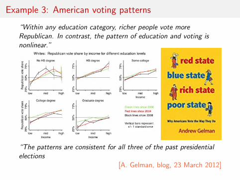
Example 3: American voting patterns
“Within any education category, richer people vote moreRepublican. In contrast, the pattern of education and voting isnonlinear.”
[A. Gelman, blog, 23 March 2012]
Example 3: American voting patterns
“Within any education category, richer people vote moreRepublican. In contrast, the pattern of education and voting isnonlinear.”“There is no plausible way based on these data in which elites canbe considered a Democratic voting bloc. To create a group ofstrongly Democratic-leaning elite whites using these graphs, youwould need to consider only postgraduates (...), and you have togo down to the below-$75,000 level of family income, which hardlyseems like the American elites to me.”
[A. Gelman, blog, 23 March 2012]
Example 3: American voting patterns
“Within any education category, richer people vote moreRepublican. In contrast, the pattern of education and voting isnonlinear.”
“The patterns are consistent for all three of the past presidentialelections
[A. Gelman, blog, 23 March 2012]
Example 4: Automatic number recognition
Reading postcodes and cheque amounts by analysing images ofdigitsClassification problem: allocate a new image (1024x1024 binaryarray) to one of the classes 0,1,...,9
Tools:
linear discriminant analysis
kernel discriminant analysis
random forests
support vector machine
deep learning
Example 5: Asian beetle invasion
Several studies in recent years have shown the harlequin conquering other ladybirds across Europe.In the UK scientists found that seven of the eight native British species have declined. Similarproblems have been encountered in Belgium and Switzerland.
[BBC News, 16 May 2013]
How did the Asian Ladybird beetlearrive in Europe?
Why do they swarm right now?
What are the routes of invasion?
How to get rid of them(biocontrol)?
[Estoup et al., 2012, Molecular Ecology Res.]
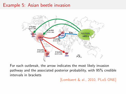
Example 5: Asian beetle invasion
For each outbreak, the arrow indicates the most likely invasionpathway and the associated posterior probability, with 95% credibleintervals in brackets
[Lombaert & al., 2010, PLoS ONE]
Example 5: Asian beetle invasion
Most likely scenario of evolution, based on data:samples from five populations (18 to 35 diploid individuals persample), genotyped at 18 autosomal microsatellite loci,summarised into 130 statistics
[Lombaert & al., 2010, PLoS ONE]
Example 6: Are more babies born on Valentine’s day thanon Halloween?
Uneven pattern of birth rate across the calendar year
with large variations on heavily significant dates (Halloween,Valentine’s day, April fool’s day, Christmas, ...)
Example 6: Are more babies born on Valentine’s day thanon Halloween?
Uneven pattern of birth rate across the calendar year with largevariations on heavily significant dates (Halloween, Valentine’s day,April fool’s day, Christmas, ...)
The data could be cleaned even further. Here’s how I’dstart: go back to the data for all the years and fit aregression with day-of-week indicators (Monday, Tuesday,etc), then take the residuals from that regression andpipe them back into [my] program to make a cleaned-upgraph. It’s well known that births are less frequent on theweekends, and unless your data happen to be an exact28-year period, you’ll get imbalance, which I’m guessingis driving a lot of the zigzagging in the graph above.
Example 6: Are more babies born on Valentine’s day thanon Halloween?
I modeled the data with a Gaussianprocess with six components:
1 slowly changing trend
2 7 day periodical componentcapturing day of week effect
3 365.25 day periodical componentcapturing day of year effect
4 component to take into accountthe special days and interactionwith weekends
5 small time scale correlating noise
6 independent Gaussian noise
[A. Gelman, blog, 12 June 2012]
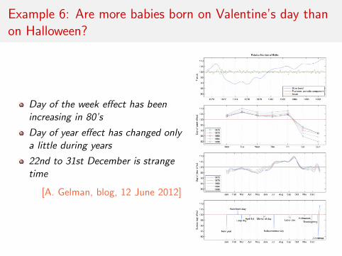
Example 6: Are more babies born on Valentine’s day thanon Halloween?
Day of the week effect has beenincreasing in 80’s
Day of year effect has changed onlya little during years
22nd to 31st December is strangetime
[A. Gelman, blog, 12 June 2012]
Example 6: Are more babies born on Valentine’s day thanon Halloween?
Day of the week effect has beenincreasing in 80’s
Day of year effect has changed onlya little during years
22nd to 31st December is strangetime
[A. Gelman, blog, 12 June 2012]
Example 7: Were the earlier Iranian elections rigged?
Presidential elections of 2009 in Iran saw Mahmoud Ahmadinejadre-elected, amidst considerable protests against rigging.
...We’ll concentrate on vote counts–the number of votesreceived by different candidates in different provinces–andin particular the last and second-to-last digits of thesenumbers. For example, if a candidate received 14,579votes in a province (...), we’ll focus on digits 7 and 9.[B. Beber & A. Scacco, The Washington Post, June 20, 2009]
Example 7: Were the earlier Iranian elections rigged?
Presidential elections of 2009 in Iran saw Mahmoud Ahmadinejadre-elected, amidst considerable protests against rigging.
The ministry provided data for 29 provinces, and weexamined the number of votes each of the four maincandidates–Ahmadinejad, Mousavi, Karroubi and MohsenRezai–is reported to have received in each of theprovinces–a total of 116 numbers.Similar analyses in other countries like Russia (2018)[B. Beber & A. Scacco, The Washington Post, June 20, 2009]
Example 7: Were the earlier Iranian elections rigged?
Presidential elections of 2009 in Iran saw Mahmoud Ahmadinejadre-elected, amidst considerable protests against rigging.
The numbers look suspicious. We find too many 7s andnot enough 5s in the last digit. We expect each digit (0,1, 2, and so on) to appear at the end of 10 percent ofthe vote counts. But in Iran’s provincial results, the digit7 appears 17 percent of the time, and only 4 percent ofthe results end in the number 5. Two such departuresfrom the average–a spike of 17 percent or more in onedigit and a drop to 4 percent or less in another–areextremely unlikely. Fewer than four in a hundrednon-fraudulent elections would produce such numbers.[B. Beber & A. Scacco, The Washington Post, June 20, 2009]
Why?
Transforming (potentially deterministic) observations of aphenomenon “into” a model allows for
detection of recurrent or rare patterns (outliers)
identification of homogeneous groups (classification) and ofchanges
selection of the most adequate scientific model or theory
assessment of the significance of an effect (statistical test)
comparison of treatments, populations, regimes, trainings, ...
estimation of non-linear regression functions
construction of dependence graphs and evaluation ofconditional independence
Assumptions
Statistical analysis is always conditional to some mathematicalassumptions on the underlying data like, e.g.,
random sampling
independent and identically distributed observations
exchangeability
stationary
weakly stationary
homocedasticity
data missing at random
When those assumptions fail to hold, statistical procedures areunreliableWarning: This does not mean statistical methodology only applieswhen the model is correct
Role of mathematics wrt statistics
Warning: This does not mean statistical methodology only applieswhen the model is correctStatistics is not [solely] a branch of mathematics, but relies onmathematics to
build probabilistic models
construct procedures as optimising criteria
validate procedures as asymptotically correct
provide a measure of confidence in the reported results
Six quotes from Kaiser Fung
You may think you have all of the data. You don’t.
One of the biggest myths of Big Data is that data aloneproduce complete answers.
Their “data” have done no arguing; it is the humans who aremaking this claim.
Before getting into the methodological issues, one needs toask the most basic question. Did the researchers check thequality of the data or just take the data as is?
We are not saying that statisticians should not tell stories.Story-telling is one of our responsibilities. What we want tosee is a clear delineation of what is data-driven and what istheory (i.e., assumptions).
[Kaiser Fung, Big Data, Plainly Spoken blog]
Six quotes from Kaiser Fung
Their “data” have done no arguing; it is the humans who aremaking this claim.
Before getting into the methodological issues, one needs toask the most basic question. Did the researchers check thequality of the data or just take the data as is?
We are not saying that statisticians should not tell stories.Story-telling is one of our responsibilities. What we want tosee is a clear delineation of what is data-driven and what istheory (i.e., assumptions).
The standard claim is that the observed effect is so large as toobviate the need for having a representative sample. Sorry —the bad news is that a huge effect for a tiny non-randomsegment of a large population can coexist with no effect forthe entire population.
[Kaiser Fung, Big Data, Plainly Spoken blog]
Chapter 1 :statistical vs. real models
Statistical modelsQuantities of interestExponential families
Statistical models
For most of the course, we assume that the data is a randomsample x1, . . . , xn and that
X1, . . . ,Xn ∼ F(x)
as i.i.d. variables or as transforms of i.i.d. variables[observations versus Random Variables]
Motivation:
Repetition of observations increases information about F, by virtueof probabilistic limit theorems (LLN, CLT)
Statistical models
For most of the course, we assume that the data is a randomsample x1, . . . , xn and that
X1, . . . ,Xn ∼ F(x)
as i.i.d. variables or as transforms of i.i.d. variables
Motivation:
Repetition of observations increases information about F, by virtueof probabilistic limit theorems (LLN, CLT)
Warning 1: Some aspects of F may ultimately remain unavailable
Statistical models
For most of the course, we assume that the data is a randomsample x1, . . . , xn and that
X1, . . . ,Xn ∼ F(x)
as i.i.d. variables or as transforms of i.i.d. variables
Motivation:
Repetition of observations increases information about F, by virtueof probabilistic limit theorems (LLN, CLT)
Warning 2: The model is always wrong, even though we behave asif...
Limit of averages
Case of an iid sequence X1, . . . ,Xn ∼ N(0, 1)
Evolution of the range of Xn across 1000 repetitions, along with one randomsequence and the theoretical 95% range
Limit theorems
Law of Large Numbers (LLN)
If X1, . . . ,Xn are i.i.d. random variables, with a well-definedexpectation E[X]
X1 + . . . + Xnn
prob−→ E[X]
[proof: see Terry Tao’s “What’s new”, 18 June 2008]
Limit theorems
Law of Large Numbers (LLN)
If X1, . . . ,Xn are i.i.d. random variables, with a well-definedexpectation E[X]
X1 + . . . + Xnn
a.s.−→ E[X]
[proof: see Terry Tao’s “What’s new”, 18 June 2008]
Limit theorems
Law of Large Numbers (LLN)
If X1, . . . ,Xn are i.i.d. random variables, with a well-definedexpectation E[X]
X1 + . . . + Xnn
a.s.−→ E[X]
Central Limit Theorem (CLT)
If X1, . . . ,Xn are i.i.d. random variables, with a well-definedexpectation E[X] and a finite variance σ2 = var(X),
√n
X1 + . . . + Xn
n− E[X]
dist.−→ N(0,σ2)
[proof: see Terry Tao’s “What’s new”, 5 January 2010]
Limit theorems
Central Limit Theorem (CLT)
If X1, . . . ,Xn are i.i.d. random variables, with a well-definedexpectation E[X] and a finite variance σ2 = var(X),
√n
X1 + . . . + Xn
n− E[X]
dist.−→ N(0,σ2)
[proof: see Terry Tao’s “What’s new”, 5 January 2010]
Continuity Theorem
IfXn
dist.−→ a
and g is continuous at a, then
g(Xn)dist.−→ g(a)
Limit theorems
Central Limit Theorem (CLT)
If X1, . . . ,Xn are i.i.d. random variables, with a well-definedexpectation E[X] and a finite variance σ2 = var(X),
√n
X1 + . . . + Xn
n− E[X]
dist.−→ N(0,σ2)
[proof: see Terry Tao’s “What’s new”, 5 January 2010]
Slutsky’s Theorem
If Xn, Yn, Zn converge in distribution to X, a, and b, respectively,then
XnYn + Zndist.−→ aX+ b
Limit theorems
Central Limit Theorem (CLT)
If X1, . . . ,Xn are i.i.d. random variables, with a well-definedexpectation E[X] and a finite variance σ2 = var(X),
√n
X1 + . . . + Xn
n− E[X]
dist.−→ N(0,σ2)
[proof: see Terry Tao’s “What’s new”, 5 January 2010]
Delta method’s Theorem
If √nXn − µ
dist.−→ Np(0,Ω)
and g : Rp → Rq is a continuously differentiable function on aneighbourhood of µ ∈ Rp, with a non-zero gradient ∇g(µ), then
√n g(Xn) − g(µ)
dist.−→ Nq(0,∇g(µ)TΩ∇g(µ))
Entertaining read
Exemple 1: Binomial sample
Case # 1: Observation of i.i.d. Bernoulli variables
Xi ∼ B(p)
with unknown parameter p (e.g., opinion poll)Case # 2: Observation of independent Bernoulli variables
Xi ∼ B(pi)
with unknown and different parameters pi (e.g., opinion poll, fluepidemics)Transform of i.i.d. U1, . . . ,Un:
Xi = I(Ui 6 pi)
Exemple 1: Binomial sample
Case # 1: Observation of i.i.d. Bernoulli variables
Xi ∼ B(p)
with unknown parameter p (e.g., opinion poll)Case # 2: Observation of conditionally independent Bernoullivariables
Xi|zi ∼ B(p(zi))
with covariate-driven parameters p(zi) (e.g., opinion poll, fluepidemics)Transform of i.i.d. U1, . . . ,Un:
Xi = I(Ui 6 pi)
Parametric versus non-parametric
Two classes of statistical models:
Parametric when F varies within a family of distributionsindexed by a parameter θ that belongs to a finite dimensionspace Θ:
F ∈ Fθ, θ ∈ Θ
and to “know” F is to know which θ it corresponds to(identifiability);
Non-parametric all other cases, i.e. when F is not constrainedin a parametric way or when only some aspects of F are ofinterest for inference
Trivia: Machine-learning does not draw such a strict distinctionbetween classes
Non-parametric models
In non-parametric models, there may still be constraints on therange of F‘s as for instance
EF[Y|X = x] = Ψ(βTx), varF(Y|X = x) = σ2
in which case the statistical inference only deals with estimating ortesting the constrained aspects or providing prediction.Note: Estimating a density or a regression function like Ψ(βTx) isonly of interest in a restricted number of cases
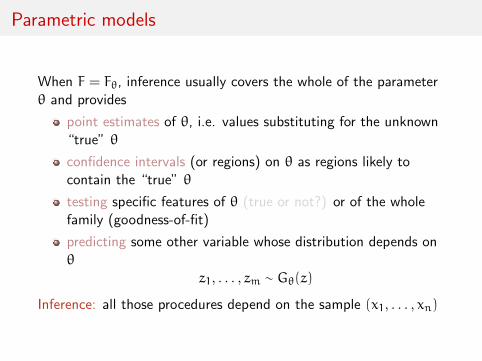
Parametric models
When F = Fθ, inference usually covers the whole of the parameterθ and provides
point estimates of θ, i.e. values substituting for the unknown“true” θ
confidence intervals (or regions) on θ as regions likely tocontain the “true” θ
testing specific features of θ (true or not?) or of the wholefamily (goodness-of-fit)
predicting some other variable whose distribution depends onθ
z1, . . . , zm ∼ Gθ(z)
Inference: all those procedures depend on the sample (x1, . . . , xn)
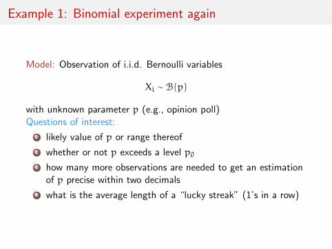
Example 1: Binomial experiment again
Model: Observation of i.i.d. Bernoulli variables
Xi ∼ B(p)
with unknown parameter p (e.g., opinion poll)Questions of interest:
1 likely value of p or range thereof
2 whether or not p exceeds a level p03 how many more observations are needed to get an estimation
of p precise within two decimals
4 what is the average length of a “lucky streak” (1’s in a row)
Exemple 2: Normal sample
Model: Observation of i.i.d. Normal variates
Xi ∼ N(µ,σ2)
with unknown parameters µ and σ > 0 (e.g., blood pressure)Questions of interest:
1 likely value of µ or range thereof
2 whether or not µ is above the mean η of another sampley1, . . . ,ym
3 percentage of extreme values in the next batch of m xi’s
4 how many more observations to exclude µ = 0 from likelyvalues
5 which of the xi’s are outliers
Quantities of interest
Statistical distributions (incompletely) characterised by (1-D)moments:
central moments
µ1 = E [X] =
∫xdF(x) µk = E
[(X− µ1)
k]k > 1
non-central moments
ξk = E[Xk]k > 1
α quantileP(X < ζα) = α
and (2-D) moments
cov(Xi,Xj) =
∫(xi − E[Xi])(xj − E[Xj])dF(xi, xj)
Note: For parametric models, those quantities are transforms ofthe parameter θ
Example 1: Binomial experiment again
Model: Observation of i.i.d. Bernoulli variables
Xi ∼ B(p)
Single parameter p with
E[X] = p var(X) = p(1− p)
[somewhat boring...]Median and mode
Example 1: Binomial experiment again
Model: Observation of i.i.d. Binomial variables
Xi ∼ B(n,p) P(X = k) =
(n
k
)pk(1− p)n−k
Single parameter p with
E[X] = np var(X) = np(1− p)
[somewhat less boring!]Median and mode
Example 2: Normal experiment again
Model: Observation of i.i.d. Normal variates
Xi ∼ N(µ,σ2) i = 1, . . . ,n ,
with unknown parameters µ and σ > 0 (e.g., blood pressure)
µ1 = E[X] = µ var(X) = σ2 µ3 = 0 µ4 = 3σ4
Median and mode equal to µ
Exponential families
Class of parametric densities with nice analytic properties
Start from the normal density:
ϕ(x; θ) =1√2π
expxθ− x2/2− θ2/2
=
exp−θ2/2√2π
exp xθ︸ ︷︷ ︸x meets θ
exp−x2/2
where θ and x only interact through single exponential product
Exponential families
Class of parametric densities with nice analytic properties
Definition
A parametric family of distributions on X is an exponential familyif its density with respect to a measure ν satisfies
where T(·) and τ(·) are k-dimensional functions and c(·) and h(·)are positive unidimensional functions.
Function c(·) is redundant, being defined by normalising constraint:
c(θ)−1 =
∫X
h(x) expT(x)Tτ(θ)dν(x)
Exponential families (examples)
Example 1: Binomial experiment again
Binomial variable
X ∼ B(n,p) P(X = k) =
(n
k
)pk(1− p)n−k
can be expressed as
P(X = k) = (1− p)n(n
k
)expk log(p/(1− p))
hence
c(p) = (1− p)n , h(x) =
(n
x
), T(x) = x , τ(p) = log(p/(1− p))
Exponential families (examples)
Example 1: Binomial experiment again
Binomial variable
X ∼ B(n,p) P(X = k) =
(n
k
)pk(1− p)n−k
can be expressed as
P(X = k) = (1− p)n(n
k
)expk log(p/(1− p))
hence
c(p) = (1− p)n , h(x) =
(n
x
), T(x) = x , τ(p) = log(p/(1− p))
Exponential families (examples)
Example 2: Normal experiment again
Normal variateX ∼ N(µ,σ2)
with parameter θ = (µ,σ2) and density
f(x|θ) =1√2πσ2
exp−(x− µ)2/2σ2
=1√2πσ2
exp−x2/2σ2 + xµ/σ2 − µ2/2σ2
=exp−µ2/2σ2√
2πσ2exp−x2/2σ2 + xµ/σ2
hence
c(θ) =exp−µ2/2σ2√
2πσ2, T(x) =
(x2
x
), τ(θ) =
(−1/2σ2
µ/σ2
)
natural exponential families
reparameterisation induced by the shape of the density:
Definition
In an exponential family, the natural parameter is τ(θ) and thenatural parameter space is
Θ =
τ ∈ Rk;
∫X
h(x) expT(x)Tτdν(x) <∞Example For the B(m,p) distribution, the natural parameter is
θ = logp/(1− p)
and the natural parameter space is R
regular and minimal exponential families
Possible to add and (better!) delete useless components of T :
Definition
A regular exponential family corresponds to the case where Θ is anopen set.A minimal exponential family corresponds to the case when theTi(X)’s are linearly independent, i.e.
Pθ(αTT(X) = const.) = 0 for α 6= 0 θ ∈ Θ
Also called non-degenerate exponential familyUsual assumption when working with exponential families
Illustrations
For a Normal N(µ,σ2) distribution,
f(x|µ,σ) =1√2π
1
σexp− x2/2σ2 + µ/σ2 x− µ2/2σ2
means this is a two-dimensional minimal exponential family
implies this is a three-dimensional minimal exponential family[Exercise: find C]
convexity properties
Highly regular densities
Theorem
The natural parameter space Θ of an exponential family is convexand the inverse normalising constant c−1(θ) is a convex function.
Example For B(n,p), the natural parameter space is R and theinverse normalising constant (1+ exp(θ))n is convex
convexity properties
Highly regular densities
Theorem
The natural parameter space Θ of an exponential family is convexand the inverse normalising constant c−1(θ) is a convex function.
Example For B(n,p), the natural parameter space is R and theinverse normalising constant (1+ exp(θ))n is convex
analytic properties
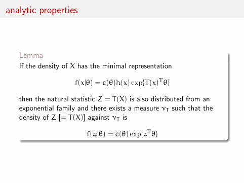
Lemma
If the density of X has the minimal representation
f(x|θ) = c(θ)h(x) expT(x)Tθ
then the natural statistic Z = T(X) is also distributed from anexponential family and there exists a measure νT such that thedensity of Z [= T(X)] against νT is
f(z; θ) = c(θ) expzTθ
analytic properties
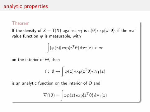
Theorem
If the density of Z = T(X) against νT is c(θ) expzTθ, if the realvalue function ϕ is measurable, with∫
|ϕ(z)| expzTθdνT (z) <∞on the interior of Θ, then
f : θ→ ∫ ϕ(z) expzTθ dνT (z)
is an analytic function on the interior of Θ and
∇f(θ) =∫zϕ(z) expzTθdνT (z)
moments of exponential families
Normalising constant c(·) generating all moments
Proposition
If T(·) : X→ Rd and the density of Z = T(X) is expzTθ−ψ(θ),then
Eθ[expT(x)Tu
]= expψ(θ+ u) −ψ(θ)
and ψ(·) is the cumulant generating function.
[Laplace transform]
moments of exponential families
Normalising constant c(·) generating all moments
Proposition
If T(·) : X→ Rd and the density of Z = T(X) is expzTθ−ψ(θ),then
Eθ[Ti(X)] =∂ψ(θ)
∂θii = 1, . . . ,d,
and
Eθ[Ti(X) Tj(X)
]=∂2ψ(θ)
∂θi∂θji, j = 1, . . . ,d
Sort of integration by part in parameter space:∫ Ti(x) +
∂
∂θilog c(θ)
c(θ)h(x) expT(x)Tθdν(x) =
∂
∂θi1 = 0
connected examples of exponential families
Example
Chi-square χ2k distribution corresponding to distribution ofX21 + . . . + X2k when Xi ∼ N(0, 1), with density
fk(z) =zk/2−1 exp−z/2
2k/2Γ(k/2)z ∈ R+
connected examples of exponential families
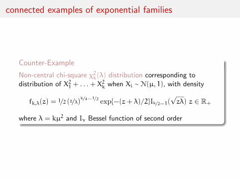
Counter-Example
Non-central chi-square χ2k(λ) distribution corresponding todistribution of X21 + . . . + X2k when Xi ∼ N(µ, 1), with density
fk,λ(z) = 1/2 (z/λ)k/4−1/2 exp−(z+ λ)/2Ik/2−1(
√zλ) z ∈ R+
where λ = kµ2 and Iν Bessel function of second order
connected examples of exponential families
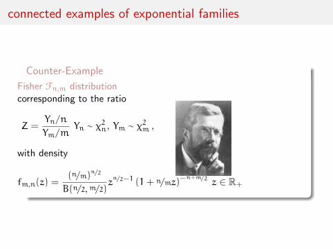
Counter-Example
Fisher Fn,m distributioncorresponding to the ratio
Z =Yn/n
Ym/mYn ∼ χ2n, Ym ∼ χ2m ,
with density
fm,n(z) =(n/m)n/2
B(n/2,m/2)zn/2−1 (1+ n/mz)−
n+m/2 z ∈ R+
connected examples of exponential families
Example
Ising Be(n/2,m/2) distribution corresponding to the distribution of
Z =nY
nY +mwhen Y ∼ Fn,m
has density
fm,n(z) =1
B(n/2,m/2)zn/2−1 (1− z)
m/2−1 z ∈ (0, 1)
connected examples of exponential families
Counter-Example
Laplace double-exponential L(µ,σ) distribution corresponding tothe rescaled difference of two exponential E(σ−1) random variables,
Z = µ+ X1 − X2 when X1,X2∼
iid E(σ−1)
has density
f(z;µ,σ) =1
σexp−σ−1|x− µ|
chapter 2 :the bootstrap method
IntroductionGlivenko-Cantelli TheoremThe Monte Carlo methodBootstrapParametric Bootstrap
Motivating example
Case of a random event with binary (Bernoulli) outcome Z ∈ 0, 1such that P(Z = 1) = pObservations z1, . . . , zn (iid) put to use to approximate p by
p = p(z1, . . . , zn) = 1/n
n∑i=1
zi
Illustration of a (moment/unbiased/maximum likelihood) estimatorof p
intrinsic statistical randomness
inference based on a random sample implies uncertainty
Since it depends on a random sample, an estimator
δ(X1, . . . ,Xn)
also is a random variable
Hence “error” in the reply: an estimator produces a differentestimation of the same quantity θ each time a new sample is used(data does produce the model)
infered variation
inference based on a random sample implies uncertainty
Question 1 :
How much does δ(X1, . . . ,Xn) vary when the sample varies?
Question 2 :
What is the variance of δ(X1, . . . ,Xn) ?
Question 3 :
What is the distribution of δ(X1, . . . ,Xn) ?
infered variation
inference based on a random sample implies uncertainty
Question 1 :
How much does δ(X1, . . . ,Xn) vary when the sample varies?
Question 2 :
What is the variance of δ(X1, . . . ,Xn) ?
Question 3 :
What is the distribution of δ(X1, . . . ,Xn) ?
infered variation
inference based on a random sample implies uncertainty
Question 1 :
How much does δ(X1, . . . ,Xn) vary when the sample varies?
Question 2 :
What is the variance of δ(X1, . . . ,Xn) ?
Question 3 :
What is the distribution of δ(X1, . . . ,Xn) ?
infered variation
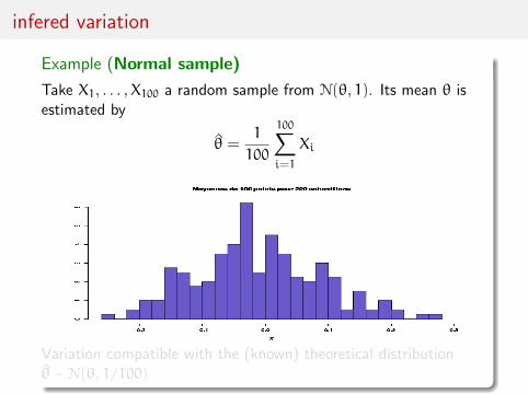
Example (Normal sample)
Take X1, . . . ,X100 a random sample from N(θ, 1). Its mean θ isestimated by
θ =1
100
100∑i=1
Xi
Variation compatible with the (known) theoretical distributionθ ∼ N(θ, 1/100)
infered variation
Example (Normal sample)
Take X1, . . . ,X100 a random sample from N(θ, 1). Its mean θ isestimated by
θ =1
100
100∑i=1
Xi
Variation compatible with the (known) theoretical distributionθ ∼ N(θ, 1/100)
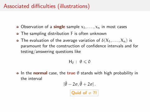
Associated difficulties (illustrations)
Observation of a single sample x1, . . . , xn in most cases
The sampling distribution F is often unknown
The evaluation of the average variation of δ(X1, . . . ,Xn) isparamount for the construction of confidence intervals and fortesting/answering questions like
H0 : θ 6 0
In the normal case, the true θ stands with high probability inthe interval
[θ− 2σ, θ+ 2σ] .
Quid of σ ?!
Estimation of the repartition function
Extension/application of the LLN to the approximation of the cdf:For an i.i.d. sample X1, . . . ,Xn, empirical cdf
Fn(x) =1
n
n∑i=1
I]−∞,x](Xi)
=card Xi; Xi 6 x
n,
Step function corresponding to the empirical distribution
1/n
n∑i=1
δXi
where δ Dirac mass
Estimation of the repartition function
Extension/application of the LLN to the approximation of the cdf:For an i.i.d. sample X1, . . . ,Xn, empirical cdf
Fn(x) =1
n
n∑i=1
I]−∞,x](Xi)
=card Xi; Xi 6 x
n,
Step function corresponding to the empirical distribution
1/n
n∑i=1
δXi
where δ Dirac mass
convergence of the empirical cdf
Glivenko-Cantelli Theorem
‖Fn − F‖∞ = supx∈R
|Fn(x) − F(x)|a.s.−→ 0
[Glivenko, 1933;Cantelli, 1933]
Fn(x) is a convergent estimator of the cdf F(x)
convergence of the empirical cdf
Dvoretzky–Kiefer–Wolfowitz inequality
P(
supx∈R
∣∣Fn(x) − F(x)∣∣ > ε) 6 e−2nε2
for every ε > εn =√1/2n ln 2
[Massart, 1990]
Fn(x) is a convergent estimator of the cdf F(x)
convergence of the empirical cdf
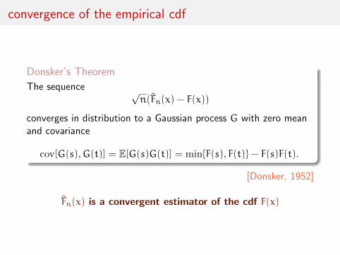
Donsker’s Theorem
The sequence √n(Fn(x) − F(x))
converges in distribution to a Gaussian process G with zero meanand covariance
Estimation of the cdf F from a normal sample of 100 pointsand variation of this estimation over 200 normal samples
Properties
Estimator of a non-parametric nature : it is not necessary toknow the distribution or the shape of the distribution of thesample to derive this estimator
Robustess versus efficiency: If the [parameterised] shape ofthe distribution is known, there exists a better approximationbased on this shape, but if the shape is wrong, the parametricresult can be completely off!
parametric versus non-parametric inference
Example (Normal sample)
cdf of N(θ, 1), Φ(x− θ)
Estimation of Φ(·− θ) by Fn and by Φ(·− θ) based on 100points and maximal variation of those estimations over 200replications
parametric versus non-parametric inference
Example (Non-normal sample)
Sample issued from
0.3N(0, 1) + 0.7N(2.5, 1)
wrongly allocated to a normal distribution Φ(·− θ)
parametric versus non-parametric inference
Estimation of F by Fn and by Φ(·− θ) based on 100 pointsand maximal variation of those estimations over 200replications
Extension to functionals of F
For any quantity θ(F) depending on F, for instance,
θ(F) =
∫h(x)dF(x) ,
[Functional of the cdf]use of the plug-in approximation θ(Fn), for instance,
θ(F) =
∫h(x)dFn(x)
= 1/n
n∑i=1
h(Xi)
[Moment estimator]
Extension to functionals of F
For any quantity θ(F) depending on F, for instance,
θ(F) =
∫h(x)dF(x) ,
[Functional of the cdf]use of the plug-in approximation θ(Fn), for instance,
θ(F) =
∫h(x)dFn(x)
= 1/n
n∑i=1
h(Xi)
[Moment estimator]
examples
variance estimator
If
θ(F) = var(X) =
∫(x− EF[X]
)2dF(x)
then
θ(Fn) =
∫(x− E
Fn[X])2
dFn(x)
= 1/n
n∑i=1
(Xi − E
Fn[X])2
= 1/n
n∑i=1
(Xi − Xn
)2which differs from the (unbiased) sample variance
1/n−1
n∑i=1
(Xi − Xn
)2
examples
median estimator
If θ(F) is the median of F, it is defined by
PF(X 6 θ(F)) = 0.5
θ(Fn) is thus defined by
PFn(X 6 θ(Fn)) = 1/n
n∑i=1
I(Xi 6 θ(Fn)) = 0.5
which implies that θ(Fn) is the median of X1, . . . ,Xn, namelyX(n/2)
median estimator
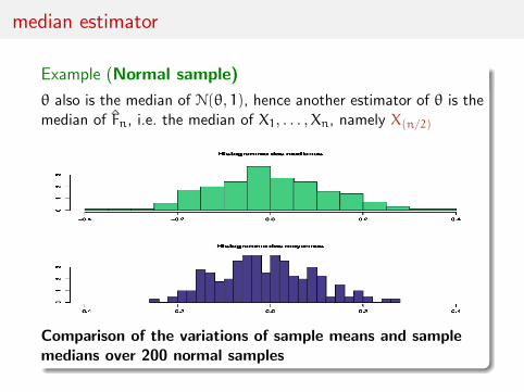
Example (Normal sample)
θ also is the median of N(θ, 1), hence another estimator of θ is themedian of Fn, i.e. the median of X1, . . . ,Xn, namely X(n/2)
Comparison of the variations of sample means and samplemedians over 200 normal samples
q-q plots
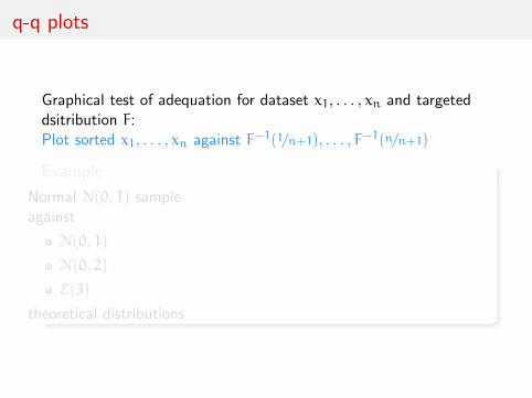
Graphical test of adequation for dataset x1, . . . , xn and targeteddsitribution F:Plot sorted x1, . . . , xn against F−1(1/n+1), . . . , F−1(n/n+1)
Example
Normal N(0, 1) sampleagainst
N(0, 1)
N(0, 2)
E(3)
theoretical distributions
q-q plots
Graphical test of adequation for dataset x1, . . . , xn and targeteddsitribution F:Plot sorted x1, . . . , xn against F−1(1/n+1), . . . , F−1(n/n+1)
Example
Normal N(0, 1) sampleagainst
N(0, 1)
N(0, 2)
E(3)
theoretical distributions
q-q plots
Graphical test of adequation for dataset x1, . . . , xn and targeteddsitribution F:Plot sorted x1, . . . , xn against F−1(1/n+1), . . . , F−1(n/n+1)
Example
Normal N(0, 1) sampleagainst
N(0, 1)
N(0, 2)
E(3)
theoretical distributions
q-q plots
Graphical test of adequation for dataset x1, . . . , xn and targeteddsitribution F:Plot sorted x1, . . . , xn against F−1(1/n+1), . . . , F−1(n/n+1)
Example
Normal N(0, 1) sampleagainst
N(0, 1)
N(0, 2)
E(3)
theoretical distributions
basis of Monte Carlo simulation
Recall the
Law of large numbers
If X1, . . . ,Xn simulated from f,
E[h(X)]n =1
n
n∑i=1
h(Xi)a.s.−→ E[h(X)]
Result fundamental for the use of computer-based simulation
basis of Monte Carlo simulation
Recall the
Law of large numbers
If X1, . . . ,Xn simulated from f,
E[h(X)]n =1
n
n∑i=1
h(Xi)a.s.−→ E[h(X)]
Result fundamental for the use of computer-based simulation
computer simulation
Principle
produce by a computer program an arbitrary long sequence
x1, x2, . . .iid∼ F
exploit the sequence as if it were a truly iid sample
Since Fn is known, it is possible to simulate from Fn, thereforeone can approximate the distribution of θ(X∗1 , . . . ,X∗n) [instead ofθ(X1, . . . ,Xn)]The distribution corresponding to
Fn(x) = card Xi; Xi 6 x/n
allocates a probability of 1/n to each point in x1, . . . , xn :
PrFn(X∗ = xi) = 1/n
Simulating from Fn is equivalent to sampling with replacement in(X1, . . . ,Xn)
[in R, sample(x,n,replace=TRUE)]
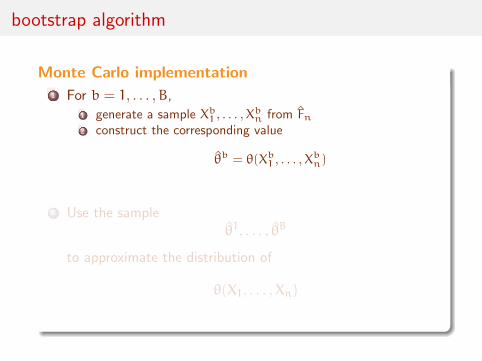
bootstrap algorithm
Monte Carlo implementation1 For b = 1, . . . ,B,
1 generate a sample Xb1 , . . . ,Xbn from Fn2 construct the corresponding value
θb = θ(Xb1 , . . . ,Xbn)
2 Use the sampleθ1, . . . , θB
to approximate the distribution of
θ(X1, . . . ,Xn)
bootstrap algorithm
Monte Carlo implementation1 For b = 1, . . . ,B,
1 generate a sample Xb1 , . . . ,Xbn from Fn2 construct the corresponding value
θb = θ(Xb1 , . . . ,Xbn)
2 Use the sampleθ1, . . . , θB
to approximate the distribution of
θ(X1, . . . ,Xn)
bootstrap algorithm
Monte Carlo implementation1 For b = 1, . . . ,B,
1 generate a sample Xb1 , . . . ,Xbn from Fn2 construct the corresponding value
θb = θ(Xb1 , . . . ,Xbn)
2 Use the sampleθ1, . . . , θB
to approximate the distribution of
θ(X1, . . . ,Xn)
mixture illustration
Observation of a sample [here simulated from0.3N(0, 1) + 0.7N(2.5, 1) as illustration]
> x=rnorm(250)+(runif(250)<.7)*2.5 #n=250
Interest in the distribution of X = 1/n∑i Xi
> xbar=mean(x)
[1] 1.73696
Bootstrap sample of X∗
> bobar=rep(0,1000) #B=1000
> for (t in 1:1000)
+ bobar[t]=mean(sample(x,250,rep=TRUE))
> hist(bobar)
mixture illustration
Example (Sample 0.3N(0, 1) + 0.7N(2.5, 1))
Variation of the empirical means over 200 bootstrap samplesversus observed average
mixture illustration
Example (Derivation of the average variation)
For an estimator θ(X1, . . . ,Xn), the standard deviation is given by
η(F) =√
EF[θ(X1, . . . ,Xn) − EF[θ(X1, . . . ,Xn)]2
]and its bootstrap approximation is
η(Fn) =
√EFn
[θ(X1, . . . ,Xn) − EFn [θ(X1, . . . ,Xn)]2
]
mixture illustration
Example (Derivation of the average variation)
For an estimator θ(X1, . . . ,Xn), the standard deviation is given by
η(F) =√
EF[θ(X1, . . . ,Xn) − EF[θ(X1, . . . ,Xn)]2
]and its bootstrap approximation is
η(Fn) =
√EFn
[θ(X1, . . . ,Xn) − EFn [θ(X1, . . . ,Xn)]2
]
mixture illustration
Example (Derivation of the average variation)
Approximation itself approximated by Monte-Carlo:
η(Fn) =
(1/B
B∑b=1
(θ(Xb1 , . . . ,Xbn) − θ)2
)1/2
where
θ = 1/B
B∑b=1
θ(Xb1 , . . . ,Xbn)
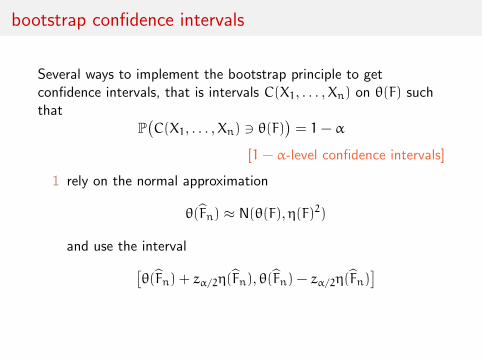
bootstrap confidence intervals
Several ways to implement the bootstrap principle to getconfidence intervals, that is intervals C(X1, . . . ,Xn) on θ(F) suchthat
P(C(X1, . . . ,Xn) 3 θ(F)
)= 1− α
[1− α-level confidence intervals]
1 rely on the normal approximation
θ(Fn) ≈ N(θ(F),η(F)2)
and use the interval[θ(Fn) + zα/2η(Fn), θ(Fn) − zα/2η(Fn)
]
bootstrap confidence intervals
Several ways to implement the bootstrap principle to getconfidence intervals, that is intervals C(X1, . . . ,Xn) on θ(F) suchthat
P(C(X1, . . . ,Xn) 3 θ(F)
)= 1− α
[1− α-level confidence intervals]
2 generate a bootstrap approximation to the cdf of θ(Fn)
H(r) = 1/B
B∑b=1
I(θ(Xb1 , . . . ,Xbn) 6 r)
and use the interval[H−1(α/2), H−1(1− α/2)
]which is also [
θ∗(nα/2), θ∗(n1−α/2)
]
bootstrap confidence intervals
Several ways to implement the bootstrap principle to getconfidence intervals, that is intervals C(X1, . . . ,Xn) on θ(F) suchthat
P(C(X1, . . . ,Xn) 3 θ(F)
)= 1− α
[1− α-level confidence intervals]
3 generate a bootstrap approximation to the cdf of θ(Fn)−θ(F),
H(r) =1
B
B∑b=1
I((θ(Xb1 , . . . ,Xbn) − θ(Fn) 6 r)
and use the interval[θ(Fn) − H
−1(1− α/2), θ(Fn) − H−1(α/2)
]which is also[
2θ(Fn) − θ∗(n1−α/2), 2θ(Fn) − θ
∗(nα/2)
]
exemple: median confidence intervals
Take X1, . . . ,Xn an iid random sample and θ(F) as the median ofF, then
θ(Fn) = X(n/2)
> x=rnorm(123)
> median(x)
[1] 0.03542237
> T=10^3
> bootmed=rep(0,T)
> for (t in 1:T) bootmed[t]=median(sample(x,123,rep=TRUE))
> sd(bootmed)
[1] 0.1222386
> median(x)-2*sd(bootmed)
[1] -0.2090547
> median(x)+2*sd(bootmed)
[1] 0.2798995
exemple: median confidence intervals
Take X1, . . . ,Xn an iid random sample and θ(F) as the median ofF, then
θ(Fn) = X(n/2)
> x=rnorm(123)
> median(x)
[1] 0.03542237
> T=10^3
> bootmed=rep(0,T)
> for (t in 1:T) bootmed[t]=median(sample(x,123,rep=TRUE))
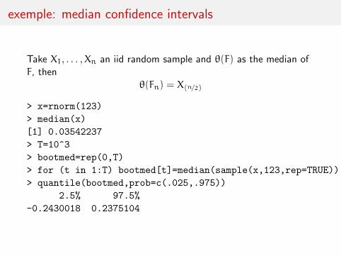
> quantile(bootmed,prob=c(.025,.975))
2.5% 97.5%
-0.2430018 0.2375104
exemple: median confidence intervals
Take X1, . . . ,Xn an iid random sample and θ(F) as the median ofF, then
θ(Fn) = X(n/2)
> x=rnorm(123)
> median(x)
[1] 0.03542237
> T=10^3
> bootmed=rep(0,T)
> for (t in 1:T) bootmed[t]=median(sample(x,123,rep=TRUE))
> 2*median(x)-quantile(bootmed,prob=c(.975,.025))
97.5% 2.5%
-0.1666657 0.3138465
example: mean bootstrap variation
Example (Sample 0.3N(0, 1) + 0.7N(2.5, 1))
Interval of bootstrap variation at ±2η(Fn) and average of theobserved sample
example: mean bootstrap variation
Example (Normal sample)
Sample
(X1, . . . ,X100)iid∼ N(θ, 1)
Comparison of the confidence intervals
[x− 2 ∗ σx/10, x+ 2 ∗ σx/10] = [−0.113, 0.327]
[normal approximation]
[x∗ − 2 ∗ σ∗, x∗ + 2 ∗ σ∗] = [−0.116, 0.336]
[normal bootstrap approximation]
[q∗(0.025),q∗(0.975)] = [−0.112, 0.336]
[generic bootstrap approximation]
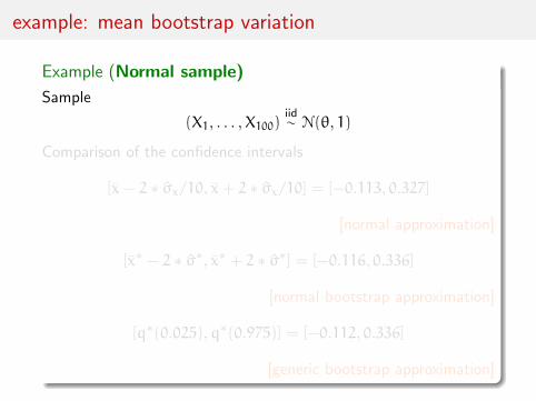
example: mean bootstrap variation
Variation ranges at 95% for a sample of 100 points and 200bootstrap replications
a counter-example
Consider X1, . . . ,Xn ∼ U(0, θ) then
θ = θ(F) = Eθ[n
n− 1X(n)
]
Using bootstrap, distribution ofn−1/nθ(Fn) far from truth
fmax(x) = nxn−1/θn I(0,θ)(x)
a counter-example
Consider X1, . . . ,Xn ∼ U(0, θ) then
θ = θ(F) = Eθ[n
n− 1X(n)
]
Using bootstrap, distribution ofn−1/nθ(Fn) far from truth
fmax(x) = nxn−1/θn I(0,θ)(x)
Parametric Bootstrap
If the parametric shape of F is known,
F(·) = Φλ(·) λ ∈ Λ ,
an evaluation of F more efficient than Fn is provided by
Φλn
where λn is a convergent estimator of λ[Cf Example 3]
Parametric Bootstrap
If the parametric shape of F is known,
F(·) = Φλ(·) λ ∈ Λ ,
an evaluation of F more efficient than Fn is provided by
Φλn
where λn is a convergent estimator of λ[Cf Example 3]
Parametric Bootstrap
Approximation of the distribution of
θ(X1, . . . ,Xn)
by the distribution of
θ(X∗1 , . . . ,X∗n) X∗1 , . . . ,X∗niid∼ Φλn
May avoid Monte Carlo simulation approximations in some cases
Parametric Bootstrap
Approximation of the distribution of
θ(X1, . . . ,Xn)
by the distribution of
θ(X∗1 , . . . ,X∗n) X∗1 , . . . ,X∗niid∼ Φλn
May avoid Monte Carlo simulation approximations in some cases
example of parametric Bootstrap
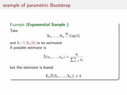
Example (Exponential Sample )
Take
X1, . . . ,Xniid∼ Exp(λ)
and λ= 1/Eλ[X] to be estimatedA possible estimator is
λ(x1, . . . , xn) =n∑ni=1 xi
but this estimator is biased
Eλ[λ(X1, . . . ,Xn)] 6= λ
example of parametric Bootstrap
Example (Exponential Sample )
Take
X1, . . . ,Xniid∼ Exp(λ)
and λ= 1/Eλ[X] to be estimatedA possible estimator is
95% variation interval for a 150 points sample with 400bootstrap replicas (top) nonparametric and (bottom)parametric
Chapter 3 :Likelihood function and inference
4 Likelihood function and inferenceThe likelihoodInformation and curvatureSufficiency and ancilarityMaximum likelihood estimationNon-regular modelsEM algorithm
The likelihood
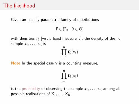
Given an usually parametric family of distributions
F ∈ Fθ, θ ∈ Θ
with densities fθ [wrt a fixed measure ν], the density of the iidsample x1, . . . , xn is
n∏i=1
fθ(xi)
Note In the special case ν is a counting measure,
n∏i=1
fθ(xi)
is the probability of observing the sample x1, . . . , xn among allpossible realisations of X1, . . . ,Xn
The likelihood
Definition (likelihood function)
The likelihood function associated with a sample x1, . . . , xn is thefunction
L :Θ −→ R+
θ −→ n∏i=1
fθ(xi)
same formula as density but different space of variation
The likelihood
Definition (likelihood function)
The likelihood function associated with a sample x1, . . . , xn is thefunction
L :Θ −→ R+
θ −→ n∏i=1
fθ(xi)
same formula as density but different space of variation
Example: density function versus likelihood function
Take the case of a Poisson density[against the counting measure]
f(x; θ) =θx
x!e−θ IN(x)
which varies in N as a function of xversus
L(θ; x) =θx
x!e−θ
which varies in R+ as a function of θ θ = 3
Example: density function versus likelihood function
Take the case of a Poisson density[against the counting measure]
f(x; θ) =θx
x!e−θ IN(x)
which varies in N as a function of xversus
L(θ; x) =θx
x!e−θ
which varies in R+ as a function of θ x = 3
Example: density function versus likelihood function
Take the case of a Normal N(0, θ)density [against the Lebesgue measure]
f(x; θ) =1√2πθ
e−x2/2θ IR(x)
which varies in R as a function of xversus
L(θ; x) =1√2πθ
e−x2/2θ
which varies in R+ as a function of θθ = 2
Example: density function versus likelihood function
Take the case of a Normal N(0, θ)density [against the Lebesgue measure]
f(x; θ) =1√2πθ
e−x2/2θ IR(x)
which varies in R as a function of xversus
L(θ; x) =1√2πθ
e−x2/2θ
which varies in R+ as a function of θx = 2
Example: density function versus likelihood function
Take the case of a Normal N(0, 1/θ)density [against the Lebesgue measure]
f(x; θ) =
√θ√2πe−x
2θ/2 IR(x)
which varies in R as a function of xversus
L(θ; x) =
√θ√2πe−x
2θ/2 IR(x)
which varies in R+ as a function of θθ = 1/2
Example: density function versus likelihood function
Take the case of a Normal N(0, 1/θ)density [against the Lebesgue measure]
f(x; θ) =
√θ√2πe−x
2θ/2 IR(x)
which varies in R as a function of xversus
L(θ; x) =
√θ√2πe−x
2θ/2 IR(x)
which varies in R+ as a function of θx = 1/2
Example: Hardy-Weinberg equilibrium
Population genetics:
Genotypes of biallelic genes AA, Aa, and aa
sample frequencies nAA, nAa and naa
multinomial model M(n;pAA,pAa,paa)
related to population proportion of A alleles, pA:
pAA = p2A , pAa = 2pA(1− pA) , paa = (1− pA)2
likelihood
L(pA|nAA,nAa,naa) ∝ p2nAAA [2pA(1− pA)]nAa(1− pA)
2naa
[Boos & Stefanski, 2013]
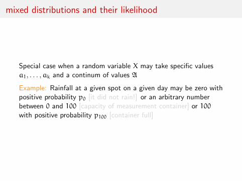
mixed distributions and their likelihood
Special case when a random variable X may take specific valuesa1, . . . ,ak and a continum of values A
Example: Rainfall at a given spot on a given day may be zero withpositive probability p0 [it did not rain!] or an arbitrary numberbetween 0 and 100 [capacity of measurement container] or 100with positive probability p100 [container full]
mixed distributions and their likelihood
Special case when a random variable X may take specific valuesa1, . . . ,ak and a continum of values A
Example: Tobit model where y ∼ N(XTβ,σ2) buty∗ = y× Iy > 0 observed
mixed distributions and their likelihood
Special case when a random variable X may take specific valuesa1, . . . ,ak and a continum of values A
Density of X against composition of two measures, counting andLebesgue:
fX(a) =
Pθ(X = a) if a ∈ a1, . . . ,ak
f(a|θ) otherwise
Results in likelihood
L(θ|x1, . . . , xn) =
k∏j=1
Pθ(X = ai)nj ×
∏xi /∈a1,...,ak
f(xi|θ)
where nj # observations equal to aj
Enters Fisher, Ronald Fisher!
Fisher’s intuition in the 20’s:
the likelihood function contains therelevant information about theparameter θ
the higher the likelihood the morelikely the parameter
the curvature of the likelihooddetermines the precision of theestimation
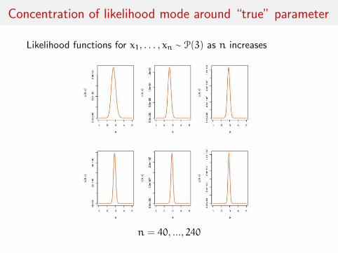
Concentration of likelihood mode around “true” parameter
Likelihood functions for x1, . . . , xn ∼ P(3) as n increases
n = 40, ..., 240
Concentration of likelihood mode around “true” parameter
Likelihood functions for x1, . . . , xn ∼ P(3) as n increases
n = 38, ..., 240
Concentration of likelihood mode around “true” parameter
Likelihood functions for x1, . . . , xn ∼ N(0, 1) as n increases
Concentration of likelihood mode around “true” parameter
Likelihood functions for x1, . . . , xn ∼ N(0, 1) as sample varies
Concentration of likelihood mode around “true” parameter
Likelihood functions for x1, . . . , xn ∼ N(0, 1) as sample varies
why concentration takes place
Consider
x1, . . . , xniid∼ F
Then
log
n∏i=1
f(xi|θ) =
n∑i=1
log f(xi|θ)
and by LLN
1/n
n∑i=1
log f(xi|θ)L−→ ∫
X
log f(x|θ)dF(x)
Lemma
Maximising the likelihood is asymptotically equivalent tominimising the Kullback-Leibler divergence∫
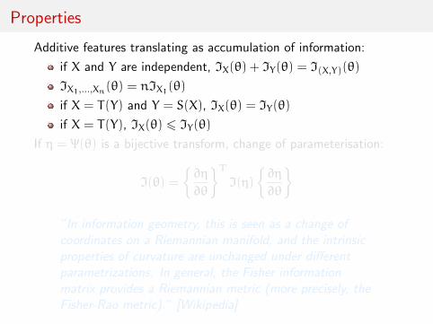
Additive features translating as accumulation of information:
if X and Y are independent, IX(θ) + IY(θ) = I(X,Y)(θ)
IX1,...,Xn(θ) = nIX1(θ)
if X = T(Y) and Y = S(X), IX(θ) = IY(θ)
if X = T(Y), IX(θ) 6 IY(θ)
If η = Ψ(θ) is a bijective transform, change of parameterisation:
I(θ) =
∂η
∂θ
T
I(η)
∂η
∂θ
”In information geometry, this is seen as a change ofcoordinates on a Riemannian manifold, and the intrinsicproperties of curvature are unchanged under differentparametrizations. In general, the Fisher informationmatrix provides a Riemannian metric (more precisely, theFisher-Rao metric).” [Wikipedia]
Properties
If η = Ψ(θ) is a bijective transform, change of parameterisation:
I(θ) =
∂η
∂θ
T
I(η)
∂η
∂θ
”In information geometry, this is seen as a change ofcoordinates on a Riemannian manifold, and the intrinsicproperties of curvature are unchanged under differentparametrizations. In general, the Fisher informationmatrix provides a Riemannian metric (more precisely, theFisher-Rao metric).” [Wikipedia]
Central limit law of the score vectorGiven X1, . . . ,Xn i.i.d. f(x|θ),
1/√n∇ log L(θ|X1, . . . ,Xn) ≈ N (0, IX1(θ))
[at the “true” θ]
Notation I1(θ) stands for IX1(θ) and indicates informationassociated with a single observation
First CLT
Central limit law of the score vectorGiven X1, . . . ,Xn i.i.d. f(x|θ),
1/√n∇ log L(θ|X1, . . . ,Xn) ≈ N (0, IX1(θ))
[at the “true” θ]
Notation I1(θ) stands for IX1(θ) and indicates informationassociated with a single observation
Sufficiency
What if a transform of the sample
S(X1, . . . ,Xn)
contains all the information, i.e.
I(X1,...,Xn)(θ) = IS(X1,...,Xn)(θ)
uniformly in θ?
In this case S(·) is called a sufficient statistic [because it issufficient to know the value of S(x1, . . . , xn) to get completeinformation]
[A statistic is an arbitrary transform of the data X1, . . . ,Xn]
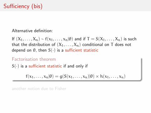
Sufficiency (bis)
Alternative definition:
If (X1, . . . ,Xn) ∼ f(x1, . . . , xn|θ) and if T = S(X1, . . . ,Xn) is suchthat the distribution of (X1, . . . ,Xn) conditional on T does notdepend on θ, then S(·) is a sufficient statistic
If (X1, . . . ,Xn) ∼ f(x1, . . . , xn|θ) and if T = S(X1, . . . ,Xn) is suchthat the distribution of (X1, . . . ,Xn) conditional on T does notdepend on θ, then S(·) is a sufficient statistic
If (X1, . . . ,Xn) ∼ f(x1, . . . , xn|θ) and if T = S(X1, . . . ,Xn) is suchthat the distribution of (X1, . . . ,Xn) conditional on T does notdepend on θ, then S(·) is a sufficient statistic
Both previous examples belong to exponential families
f(x|θ) = h(x) expT(θ)TS(x) − τ(θ)
Generic property of exponential families:
f(x1, . . . , xn|θ) =
n∏i=1
h(xi) exp
T(θ)T
n∑i=1
S(xi) − nτ(θ)
lemma
For an exponential family with summary statistic S(·), the statistic
S(X1, . . . ,Xn) =
n∑i=1
S(Xi)
is sufficient
Sufficiency and exponential families
Both previous examples belong to exponential families
f(x|θ) = h(x) expT(θ)TS(x) − τ(θ)
Generic property of exponential families:
f(x1, . . . , xn|θ) =
n∏i=1
h(xi) exp
T(θ)T
n∑i=1
S(xi) − nτ(θ)
lemma
For an exponential family with summary statistic S(·), the statistic
S(X1, . . . ,Xn) =
n∑i=1
S(Xi)
is sufficient
Sufficiency as a rare feature
Nice property reducing the data to a low dimension transform but...
How frequent is it within the collection of probability distributions?
Very rare as essentially restricted to exponential families[Pitman-Koopman-Darmois theorem]
with the exception of parameter-dependent families like U(0, θ)
Pitman-Koopman-Darmois characterisation
If X1, . . . ,Xn are iid random variables from a densityf(·|θ) whose support does not depend on θ and verifyingthe property that there exists an integer n0 such that, forn > n0, there is a sufficient statistic S(X1, . . . ,Xn) withfixed [in n] dimension, then f(·|θ) belongs to anexponential family
[Factorisation theorem]
Note: Darmois published this result in 1935 [in French] andKoopman and Pitman in 1936 [in English] but Darmois is generallyomitted from the theorem... Fisher proved it for one-D sufficientstatistics in 1934
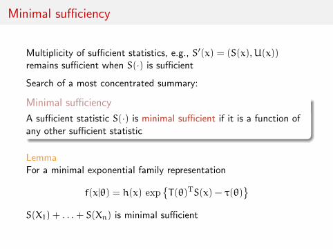
Minimal sufficiency
Multiplicity of sufficient statistics, e.g., S′(x) = (S(x),U(x))remains sufficient when S(·) is sufficient
Search of a most concentrated summary:
Minimal sufficiency
A sufficient statistic S(·) is minimal sufficient if it is a function ofany other sufficient statistic
LemmaFor a minimal exponential family representation
f(x|θ) = h(x) expT(θ)TS(x) − τ(θ)
S(X1) + . . . + S(Xn) is minimal sufficient
Minimal sufficiency
Multiplicity of sufficient statistics, e.g., S′(x) = (S(x),U(x))remains sufficient when S(·) is sufficient
Search of a most concentrated summary:
Minimal sufficiency
A sufficient statistic S(·) is minimal sufficient if it is a function ofany other sufficient statistic
LemmaFor a minimal exponential family representation
f(x|θ) = h(x) expT(θ)TS(x) − τ(θ)
S(X1) + . . . + S(Xn) is minimal sufficient
Ancillarity
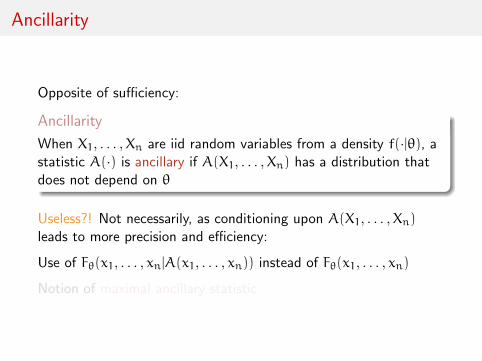
Opposite of sufficiency:
Ancillarity
When X1, . . . ,Xn are iid random variables from a density f(·|θ), astatistic A(·) is ancillary if A(X1, . . . ,Xn) has a distribution thatdoes not depend on θ
Useless?! Not necessarily, as conditioning upon A(X1, . . . ,Xn)leads to more precision and efficiency:
Use of Fθ(x1, . . . , xn|A(x1, . . . , xn)) instead of Fθ(x1, . . . , xn)
Notion of maximal ancillary statistic
Ancillarity
Opposite of sufficiency:
Ancillarity
When X1, . . . ,Xn are iid random variables from a density f(·|θ), astatistic A(·) is ancillary if A(X1, . . . ,Xn) has a distribution thatdoes not depend on θ
Useless?! Not necessarily, as conditioning upon A(X1, . . . ,Xn)leads to more precision and efficiency:
Use of Fθ(x1, . . . , xn|A(x1, . . . , xn)) instead of Fθ(x1, . . . , xn)
3 If X1, . . . ,Xniid∼ f(x|θ), rank(X1, . . . ,Xn) is ancillary
> x=rnorm(10)
> rank(x)
[1] 7 4 1 5 2 6 8 9 10 3
[see, e.g., rank tests]
Basu’s theorem
Completeness
When X1, . . . ,Xn are iid random variables from a density f(·|θ), astatistic A(·) is complete if the only function Ψ such thatEθ[Ψ(A(X1, . . . ,Xn))] = 0 for all θ’s is the null function
Let X = (X1, . . . ,Xn) be a random sample from f(·|θ) whereθ ∈ Θ. If V is an ancillary statistic, and T is complete andsufficient for θ then T and V are independent with respect to f(·|θ)for all θ ∈ Θ.
[Basu, 1955]
some examples
Example 1
If X = (X1, . . . ,Xn) is a random sample from the Normaldistribution N(µ,σ2) when σ is known, Xn = 1/n
∑ni=1 Xi is
sufficient and complete, while (X1 − Xn, . . . ,Xn − Xn) is ancillary,hence independent from Xn.
counter-Example 2
Let N be an integer-valued random variable with known pdf(π1,π2, . . .). And let S|N = n ∼ B(n,p) with unknown p. Then(N,S) is minimal sufficient and N is ancillary.
more counterexamples
counter-Example 3
If X = (X1, . . . ,Xn) is a random sample from the doubleexponential distribution f(x|θ) = 2 exp−|x− θ|, (X(1), . . . ,X(n))is minimal sufficient but not complete since X(n) − X(1) is ancillaryand with fixed expectation.
counter-Example 4
If X is a random variable from the Uniform U(θ, θ+ 1)distribution, X and [X] are independent, but while X is completeand sufficient, [X] is not ancillary.
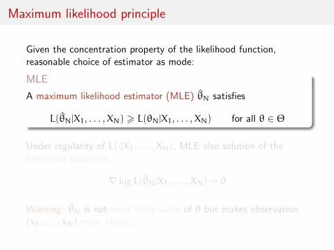
Given the concentration property of the likelihood function,reasonable choice of estimator as mode:
MLE
A maximum likelihood estimator (MLE) θN satisfies
L(θN|X1, . . . ,XN) > L(θN|X1, . . . ,XN) for all θ ∈ Θ
Under regularity of L(·|X1, . . . ,XN), MLE also solution of thelikelihood equations
∇ log L(θN|X1, . . . ,XN) = 0
Warning: θN is not most likely value of θ but makes observation(x1, . . . , xN) most likely...
Maximum likelihood principle
Given the concentration property of the likelihood function,reasonable choice of estimator as mode:
MLE
A maximum likelihood estimator (MLE) θN satisfies
L(θN|X1, . . . ,XN) > L(θN|X1, . . . ,XN) for all θ ∈ Θ
Under regularity of L(·|X1, . . . ,XN), MLE also solution of thelikelihood equations
∇ log L(θN|X1, . . . ,XN) = 0
Warning: θN is not most likely value of θ but makes observation(x1, . . . , xN) most likely...
Maximum likelihood invariance
Principle independent of parameterisation:
If ξ = h(θ) is a one-to-one transform of θ, then
ξMLEN = h(θMLE
N )
[estimator of transform = transform of estimator]
By extension, if ξ = h(θ) is any transform of θ, then
ξMLEN = h(θMLE
n )
Alternative of profile likelihoods distinguishing between parametersof interest and nuisance parameters
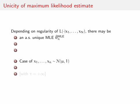
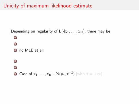
Unicity of maximum likelihood estimate
Depending on regularity of L(·|x1, . . . , xN), there may be
1 an a.s. unique MLE θMLEn
2
3
1 Case of x1, . . . , xn ∼ N(µ, 1)
2
3 [with τ = +∞]
Unicity of maximum likelihood estimate
Depending on regularity of L(·|x1, . . . , xN), there may be
1
2 several or an infinity of MLE’s [or of solutions to likelihoodequations]
3
1
2 Case of x1, . . . , xn ∼ N(µ1 + µ2, 1) [and mixtures of normal]
3 [with τ = +∞]
Unicity of maximum likelihood estimate
Depending on regularity of L(·|x1, . . . , xN), there may be
1
2
3 no MLE at all
1
2
3 Case of x1, . . . , xn ∼ N(µi, τ−2) [with τ = +∞]
Unicity of maximum likelihood estimate
Consequence of standard differential calculus results on`(θ) = log L(θ|x1, . . . , xn):
lemma
If Θ is connected and open, and if `(·) is twice-differentiable with
limθ→∂Θ `(θ) < +∞
and if H(θ) = ∇∇T`(θ) is positive definite at all solutions of thelikelihood equations, then `(·) has a unique global maximum
Limited appeal because excluding local maxima
Unicity of MLE for exponential families
lemma
If f(·|θ) is a minimal exponential family
f(x|θ) = h(x) expT(θ)TS(x) − τ(θ)
with T(·) one-to-one and twice differentiable over Θ, if Θ is open,and if there is at least one solution to the likelihood equations,then it is the unique MLE
Likelihood equation is equivalent to S(x) = Eθ[S(X)]
Unicity of MLE for exponential families
lemma
If Θ is connected and open, and if `(·) is twice-differentiable with
limθ→∂Θ `(θ) < +∞
and if H(θ) = ∇∇T`(θ) is positive definite at all solutions of thelikelihood equations, then `(·) has a unique global maximum
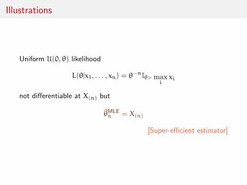
Illustrations
Uniform U(0, θ) likelihood
L(θ|x1, . . . , xn) = θ−nIθ> max
ixi
not differentiable at X(n) but
θMLEn = X(n)
[Super-efficient estimator]
Illustrations
Bernoulli B(p) likelihood
L(p|x1, . . . , xn) = p/1−p∑i xi (1− p)n
differentiable over (0, 1) and
pMLEn = Xn
Illustrations
Normal N(µ,σ2) likelihood
L(µ,σ|x1, . . . , xn) ∝ σ−n exp
−1
2σ2
n∑i=1
(xi − xn)2 −
1
2σ2
n∑i=1
(xn − µ)2
differentiable with
(µMLEn , σ2
MLE
n ) =
(Xn,
1
n
n∑i=1
(Xi − Xn)2
)
The fundamental theorem of Statistics
fundamental theorem
Under appropriate conditions, if (X1, . . . ,Xn)iid∼ f(x|θ), if θn is
solution of ∇ log f(X1, . . . ,Xn|θ) = 0, then
√nθn − θ
L−→ Np(0, I(θ)−1)
Equivalent of CLT for estimation purposes
I(θ) can be replaced with I(θn)
or even I(θn) = −1/n∑i∇∇T log f(xi|θn)
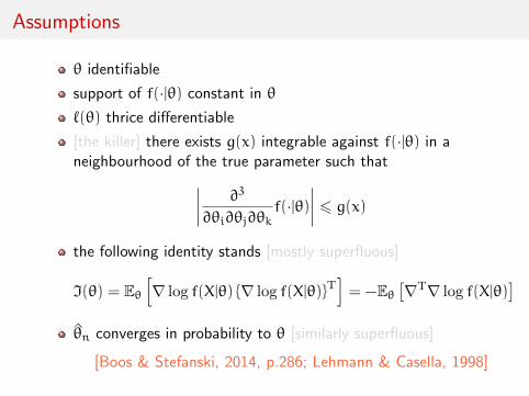
Assumptions
θ identifiable
support of f(·|θ) constant in θ
`(θ) thrice differentiable
[the killer] there exists g(x) integrable against f(·|θ) in aneighbourhood of the true parameter such that∣∣∣∣ ∂3
∂θi∂θj∂θkf(·|θ)
∣∣∣∣ 6 g(x)the following identity stands [mostly superfluous]
I(θ) = Eθ[∇ log f(X|θ) ∇ log f(X|θ)T
]= −Eθ
[∇T∇ log f(X|θ)
]θn converges in probability to θ [similarly superfluous]
for any θ0, with integration operated against conditionnaldistribution of Z given observables (and parameters), k(z|θ0, x)
[A tale of] two θ’s
There are “two θ’s” ! : in (1), θ0 is a fixed (and arbitrary) valuedriving integration, while θ both free (and variable)
Maximising observed likelihood
L(θ|x)
equivalent to maximise r.h.s. term in (1)
E[log Lc(θ|x,Z)|θ0, x] − E[log k(Z|θ, x)|θ0, x]
[A tale of] two θ’s
There are “two θ’s” ! : in (1), θ0 is a fixed (and arbitrary) valuedriving integration, while θ both free (and variable)
Maximising observed likelihood
L(θ|x)
equivalent to maximise r.h.s. term in (1)
E[log Lc(θ|x,Z)|θ0, x] − E[log k(Z|θ, x)|θ0, x]
Intuition for EM
Instead of maximising wrt θ r.h.s. term in (1), maximise only
E[log Lc(θ|x,Z)|θ0, x]
Maximisation of complete log-likelihood impossible since z
unknown, hence substitute by maximisation of expected completelog-likelihood, with expectation depending on term θ0
Intuition for EM
Instead of maximising wrt θ r.h.s. term in (1), maximise only
E[log Lc(θ|x,Z)|θ0, x]
Maximisation of complete log-likelihood impossible since z
unknown, hence substitute by maximisation of expected completelog-likelihood, with expectation depending on term θ0
Expectation–Maximisation
Expectation of complete log-likelihood denoted
Q(θ|θ0, x) = E[log Lc(θ|x,Z)|θ0, x]
to stress dependence on θ0 and sample x
Principle
EM derives sequence of estimators θ(j), j = 1, 2, . . ., throughiteration of Expectation and Maximisation steps:
Q(θ(j)|θ(j−1), x) = maxθQ(θ|θ(j−1), x).
EM Algorithm
Iterate (in m)
1 (step E) Compute
Q(θ|θ(m), x) = E[log Lc(θ|x,Z)|θ(m), x] ,
2 (step M) Maximise Q(θ|θ(m), x) in θ and set
θ(m+1) = arg maxθ
Q(θ|θ(m), x).
until a fixed point [of Q] is found[Dempster, Laird, & Rubin, 1978]
Justification
Observed likelihoodL(θ|x)
increases at every EM step
L(θ(m+1)|x) > L(θ(m)|x)
[Exercice: use Jensen and (1)]
Censored data
Normal N(θ, 1) sample right-censored
L(θ|x) =1
(2π)m/2exp
−1
2
m∑i=1
(xi − θ)2
[1−Φ(a− θ)]n−m
Associated complete log-likelihood:
log Lc(θ|x, z) ∝ −1
2
m∑i=1
(xi − θ)2 −
1
2
n∑i=m+1
(zi − θ)2 ,
where zi’s are censored observations, with density
k(z|θ, x) =exp− 1
2(z− θ)2
√2π[1−Φ(a− θ)]
=ϕ(z− θ)
1−Φ(a− θ), a < z.
Censored data (2)
At j-th EM iteration
Q(θ|θ(j), x) ∝ −1
2
m∑i=1
(xi − θ)2 −
1
2E
[n∑
i=m+1
(Zi − θ)2
∣∣∣∣∣ θ(j), x]
∝ −1
2
m∑i=1
(xi − θ)2
−1
2
n∑i=m+1
∫∞a
(zi − θ)2k(z|θ(j), x)dzi
Censored data (3)
Differenciating in θ,
n θ(j+1) = mx+ (n−m)E[Z|θ(j)] ,
with
E[Z|θ(j)] =∫∞a
zk(z|θ(j), x)dz = θ(j) +ϕ(a− θ(j))
1−Φ(a− θ(j)).
Hence, EM sequence provided by
θ(j+1) =m
nx+
n−m
n
[θ(j) +
ϕ(a− θ(j))
1−Φ(a− θ(j))
],
which converges to likelihood maximum θ
Censored data (3)
Differenciating in θ,
n θ(j+1) = mx+ (n−m)E[Z|θ(j)] ,
with
E[Z|θ(j)] =∫∞a
zk(z|θ(j), x)dz = θ(j) +ϕ(a− θ(j))
1−Φ(a− θ(j)).
Hence, EM sequence provided by
θ(j+1) =m
nx+
n−m
n
[θ(j) +
ϕ(a− θ(j))
1−Φ(a− θ(j))
],
which converges to likelihood maximum θ
Mixtures
Mixture of two normal distributions with unknown means
.3N1(µ0, 1) + .7N1(µ1, 1),
sample X1, . . . ,Xn and parameter θ = (µ0,µ1)Missing data: Zi ∈ 0, 1, indicator of component associated withXi ,
Xi|zi ∼ N(µzi , 1) Zi ∼ B(.7)
Complete likelihood
log Lc(θ|x, z) ∝ −1
2
n∑i=1
zi(xi − µ1)2 −
1
2
n∑i=1
(1− zi)(xi − µ0)2
= −1
2n1(µ1 − µ1)
2 −1
2(n− n1)(µ0 − µ0)
2
with
n1 =
n∑i=1
zi , n1µ1 =
n∑i=1
zixi , (n− n1)µ0 =
n∑i=1
(1− zi)xi
Mixtures (2)
At j-th EM iteration
Q(θ|θ(j), x) =1
2E[n1(µ1 − µ1)
2 + (n− n1)(µ0 − µ0)2|θ(j), x
]Differenciating in θ
θ(j+1) =
E[n1µ1
∣∣θ(j), x] /E [n1|θ(j), x]E[(n− n1)µ0
∣∣θ(j), x] /E [(n− n1)|θ(j), x]
Mixtures (3)
Hence θ(j+1) given by∑ni=1 E
[Zi∣∣θ(j), xi] xi /∑n
i=1 E[Zi|θ(j), xi
]∑ni=1 E
[(1− Zi)
∣∣θ(j), xi] xi /∑ni=1 E
[(1− Zi)|θ(j), xi
]
Conclusion
Step (E) in EM replaces missing data Zi with their conditionalexpectation, given x (expectation that depend on θ(m)).
Mixtures (3)
−1 0 1 2 3
−1
01
23
µ1
µ 2
EM iterations for several starting values
Properties
EM algorithm such that
it converges to local maximum or saddle-point
it depends on the initial condition θ(0)
it requires several initial values when likelihood multimodal
Chapter 4 :Decision theory and Bayesian analysis
5 Decision theory and Bayesian analysisBayesian modellingConjugate priorsImproper prior distributionsBayesian inference
A pedestrian example
paired and orphan socks
A drawer contains an unknown number of socks, some of whichcan be paired and some of which are orphans (single). One takesat random 11 socks without replacement from this drawer: no paircan be found among those. What can we infer about the totalnumber of socks in the drawer?
sounds like an impossible task
one observation x = 11 and two unknowns, nsocks and npairs
writing the likelihood is a challenge [exercise]
A pedestrian example
paired and orphan socks
A drawer contains an unknown number of socks, some of whichcan be paired and some of which are orphans (single). One takesat random 11 socks without replacement from this drawer: no paircan be found among those. What can we infer about the totalnumber of socks in the drawer?
sounds like an impossible task
one observation x = 11 and two unknowns, nsocks and npairs
and 11 socks picked at random from S give X unique socks.
Rassmus’ reasoning
If you are a family of 3-4 persons then a guesstimate would be thatyou have something like 15 pairs of socks in store. It is alsopossible that you have much more than 30 socks. So as a prior fornsocks I’m going to use a negative binomial with mean 30 andstandard deviation 15.On npairs/2nsocks I’m going to put a Beta prior distribution that putsmost of the probability over the range 0.75 to 1.0,
2 generate a newobservation of X,number of uniquesocks out of 11.
3 accept the pair(nsocks,npairs) if therealisation of X isequal to 11
Meaning
ns
Den
sity
0 10 20 30 40 50 60
0.00
0.01
0.02
0.03
0.04
0.05
0.06
The outcome of this simulation method returns a distribution onthe pair (nsocks,npairs) that is the conditional distribution of thepair given the observation X = 11Proof: Generations from π(nsocks,npairs) are accepted with probability
P X = 11|(nsocks,npairs)
Meaning
ns
Den
sity
0 10 20 30 40 50 60
0.00
0.01
0.02
0.03
0.04
0.05
0.06
The outcome of this simulation method returns a distribution onthe pair (nsocks,npairs) that is the conditional distribution of thepair given the observation X = 11Proof: Hence accepted values distributed from
π(nsocks,npairs)× P X = 11|(nsocks,npairs) = π(nsocks,npairs|X = 11)
General principle
Bayesian principle Given a probabilitydistribution on the parameter θ calledprior
π(θ)
and an observation x of X ∼ f(x|θ),Bayesian inference relies on theconditional distribution of θ given X = x
π(θ|x) =π(θ)f(x|θ)∫π(θ)f(x|θ)dθ
called posterior distribution[Bayes’ theorem]
Thomas Bayes(FRS, 1701?-1761)
Bayesian inference
Posterior distributionπ(θ|x)
as distribution on θ the parameter conditional on x theobservation used for all aspects of inference
point estimation, e.g., E[h(θ)|x];confidence intervals, e.g.,θ; π(θ|x) > κ;
tests of hypotheses, e.g.,π(θ = 0|x) ; and
prediction of future observations
Central tool... central to Bayesian inference
Posterior defined up to a constant as
π(θ|x) ∝ f(x|θ)π(θ)
Operates conditional upon the observation(s) X = x
Integrate simultaneously prior information and informationbrought by x
Avoids averaging over the unobserved values of X
Coherent updating of the information available on θ,independent of the order in which i.i.d. observations arecollected [domino effect]
Provides a complete inferential scope and a unique motor ofinference
The thorny issue of the prior distribution
Compared with likelihood inference, based solely on
L(θ|x1, . . . , xn) =
n∏i=1
f(xi|θ)
Bayesian inference introduces an extra measure π(θ) that is chosena priori, hence subjectively by the statistician based on
hypothetical range of θ
guesstimates of θ with an associated (lack of) precision
type of sampling distribution
Note There also exist reference solutions (see below)
Bayes’ example
Billiard ball W rolled on a line of lengthone, with a uniform probability ofstopping anywhere: W stops at p.Second ball O then rolled n times underthe same assumptions. X denotes thenumber of times the ball O stopped onthe left of W.
Bayes’ example
Billiard ball W rolled on a line of lengthone, with a uniform probability ofstopping anywhere: W stops at p.Second ball O then rolled n times underthe same assumptions. X denotes thenumber of times the ball O stopped onthe left of W.
Thomas Bayes’ question
Given X, what inference can wemake on p?
Bayes’ example
Billiard ball W rolled on a line of lengthone, with a uniform probability ofstopping anywhere: W stops at p.Second ball O then rolled n times underthe same assumptions. X denotes thenumber of times the ball O stopped onthe left of W.
Modern translation:
Derive the posterior distribution of pgiven X, when
p ∼ U([0, 1]) and X ∼ B(n,p)
Resolution
Since
P(X = x|p) =
(n
x
)px(1− p)n−x,
P(a < p < b and X = x) =
∫ba
(n
x
)px(1− p)n−xdp
and
P(X = x) =
∫ 10
(n
x
)px(1− p)n−x dp,
Resolution (2)
then
P(a < p < b|X = x) =
∫ba
(nx
)px(1− p)n−x dp∫1
0
(nx
)px(1− p)n−x dp
=
∫ba p
x(1− p)n−x dp
B(x+ 1,n− x+ 1),
i.e.p|x ∼ Be(x+ 1,n− x+ 1)
[Beta distribution]
Resolution (2)
then
P(a < p < b|X = x) =
∫ba
(nx
)px(1− p)n−x dp∫1
0
(nx
)px(1− p)n−x dp
=
∫ba p
x(1− p)n−x dp
B(x+ 1,n− x+ 1),
i.e.p|x ∼ Be(x+ 1,n− x+ 1)
[Beta distribution]
Conjugate priors
Easiest case is when prior distribution is within parametric family
Conjugacy
In this case, posterior inference is tractable and reduces toupdating the hyperparameters∗ of the prior
Example In Thomas Bayes’ example, the Be(a,b) prior isconjugate
∗The hyperparameters are parameters of the priors; they are most often nottreated as random variables
Conjugate priors
Easiest case is when prior distribution is within parametric family
Conjugacy
Given a likelihood function L(y|θ), the family Π of priors π0 on Θis said to be conjugate if the posterior π(·|y) also belong to Π
In this case, posterior inference is tractable and reduces toupdating the hyperparameters∗ of the prior
Example In Thomas Bayes’ example, the Be(a,b) prior isconjugate
∗The hyperparameters are parameters of the priors; they are most often nottreated as random variables
Conjugate priors
Easiest case is when prior distribution is within parametric family
Conjugacy
A family F of probability distributions on Θ is conjugate for alikelihood function f(x|θ) if, for every π ∈ F, the posteriordistribution π(θ|x) also belongs to F.
In this case, posterior inference is tractable and reduces toupdating the hyperparameters∗ of the prior
Example In Thomas Bayes’ example, the Be(a,b) prior isconjugate
∗The hyperparameters are parameters of the priors; they are most often nottreated as random variables
Necessary extension from a prior probability distribution to a priorσ-finite positive measure π such that∫
Θ
π(θ)dθ = +∞Improper prior distribution
Note A σ-finite density with ∫Θ
π(θ)dθ < +∞can be renormalised into a probability density
Improper distributions
Necessary extension from a prior probability distribution to a priorσ-finite positive measure π such that∫
Θ
π(θ)dθ = +∞Improper prior distribution
Note A σ-finite density with ∫Θ
π(θ)dθ < +∞can be renormalised into a probability density
Improper distributions
Necessary extension from a prior probability distribution to a priorσ-finite positive measure π such that∫
Θ
π(θ)dθ = +∞Improper prior distribution
Note A σ-finite density with ∫Θ
π(θ)dθ < +∞can be renormalised into a probability density
Justifications
Often automatic prior determination leads to improper priordistributions
1 Only way to derive a prior in noninformative settings
2 Performances of estimators derived from these generalizeddistributions usually good
3 Improper priors often occur as limits of proper distributions
4 More robust answer against possible misspecifications of theprior
5 Penalization factor
Validation
Extension of the posterior distribution π(θ|x) associated with animproper prior π as given by Bayes’s formula
π(θ|x) =f(x|θ)π(θ)∫
Θ f(x|θ)π(θ)dθ,
when ∫Θ
f(x|θ)π(θ)dθ <∞
Validation
Extension of the posterior distribution π(θ|x) associated with animproper prior π as given by Bayes’s formula
π(θ|x) =f(x|θ)π(θ)∫
Θ f(x|θ)π(θ)dθ,
when ∫Θ
f(x|θ)π(θ)dθ <∞
Normal illustration
If x ∼ N(θ, 1) and π(θ) = $, constant, the pseudo marginaldistribution is
m(x) = $
∫+∞−∞
1√2π
exp−(x− θ)2/2
dθ = $
and the posterior distribution of θ is
π(θ | x) =1√2π
exp−(x−θ)2/2
,
i.e., corresponds to a N(x, 1) distribution.[independent of ω]
Normal illustration
If x ∼ N(θ, 1) and π(θ) = $, constant, the pseudo marginaldistribution is
m(x) = $
∫+∞−∞
1√2π
exp−(x− θ)2/2
dθ = $
and the posterior distribution of θ is
π(θ | x) =1√2π
exp−(x−θ)2/2
,
i.e., corresponds to a N(x, 1) distribution.[independent of ω]
Normal illustration
If x ∼ N(θ, 1) and π(θ) = $, constant, the pseudo marginaldistribution is
m(x) = $
∫+∞−∞
1√2π
exp−(x− θ)2/2
dθ = $
and the posterior distribution of θ is
π(θ | x) =1√2π
exp−(x−θ)2/2
,
i.e., corresponds to a N(x, 1) distribution.[independent of ω]
Warning
The mistake is to think of them [non-informative priors]as representing ignorance
[Lindley, 1990]
Normal illustration:Consider a θ ∼ N(0, τ2) prior. Then
limτ→∞ Pπ (θ ∈ [a,b]) = 0
for any (a,b)
Warning
Noninformative priors cannot be expected to representexactly total ignorance about the problem at hand, butshould rather be taken as reference or default priors,upon which everyone could fall back when the priorinformation is missing.
[Kass and Wasserman, 1996]
Normal illustration:Consider a θ ∼ N(0, τ2) prior. Then
limτ→∞ Pπ (θ ∈ [a,b]) = 0
for any (a,b)
Haldane prior
Consider a binomial observation, x ∼ B(n,p), and
π∗(p) ∝ [p(1− p)]−1
[Haldane, 1931]The marginal distribution,
m(x) =
∫ 10
[p(1− p)]−1(n
x
)px(1− p)n−xdp
= B(x,n− x),
is only defined for x 6= 0,n .[Not recommended!]
Haldane prior
Consider a binomial observation, x ∼ B(n,p), and
π∗(p) ∝ [p(1− p)]−1
[Haldane, 1931]The marginal distribution,
m(x) =
∫ 10
[p(1− p)]−1(n
x
)px(1− p)n−xdp
= B(x,n− x),
is only defined for x 6= 0,n .[Not recommended!]
The Jeffreys prior
Based on Fisher information
I(θ) = Eθ[∂`
∂θt∂`
∂θ
]Jeffreys prior density is
π∗(θ) ∝ |I(θ)|1/2
Pros & Cons
relates to information theory
agrees with most invariant priors
parameterisation invariant
The Jeffreys prior
Based on Fisher information
I(θ) = Eθ[∂`
∂θt∂`
∂θ
]Jeffreys prior density is
π∗(θ) ∝ |I(θ)|1/2
Pros & Cons
relates to information theory
agrees with most invariant priors
parameterisation invariant
Example
If x ∼ Np(θ, Ip), Jeffreys’ prior is
π(θ) ∝ 1
and if η = ‖θ‖2,π(η) = ηp/2−1
andEπ[η|x] = ‖x‖2 + p
with bias 2p[Not recommended!]
Example
If x ∼ B(n, θ), Jeffreys’ prior is
Be(1/2, 1/2)
and, if n ∼ Neg(x, θ), Jeffreys’ prior is
π2(θ) = −Eθ[∂2
∂θ2log f(x|θ)
]= Eθ
[x
θ2+
n− x
(1− θ)2
]=
x
θ2(1− θ),
∝ θ−1(1− θ)−1/2
MAP estimator
When considering estimates of the parameter θ, one defaultsolution is the maximum a posteriori (MAP) estimator
arg maxθ`(θ|x)π(θ)
Motivations
Most likely value of θ
Penalized likelihood estimator
Further appeal in restricted parameter spaces
MAP estimator
When considering estimates of the parameter θ, one defaultsolution is the maximum a posteriori (MAP) estimator
arg maxθ`(θ|x)π(θ)
Motivations
Most likely value of θ
Penalized likelihood estimator
Further appeal in restricted parameter spaces
Illustration
Consider x ∼ B(n,p). Possible priors:
π∗(p) =1
B(1/2, 1/2)p−1/2(1− p)−1/2 ,
π1(p) = 1 and π2(p) = p−1(1− p)−1 .
Corresponding MAP estimators:
δ∗(x) = max
(x− 1/2
n− 1, 0
),
δ1(x) =x
n,
δ2(x) = max
(x− 1
n− 2, 0
).
Illustration [opposite]
MAP not always appropriate:When
f(x|θ) =1
π
[1+ (x− θ)2
]−1,
and
π(θ) =1
2e−|θ|
then MAP estimator of θ is always
δ∗(x) = 0
Prediction
Inference on new observations depending on the same parameter,conditional on the current data
If x ∼ f(x|θ) [observed], θ ∼ π(θ), and z ∼ g(z|x, θ) [unobserved],predictive of z is marginal conditional
gπ(z|x) =
∫Θ
g(z|x, θ)π(θ|x)dθ.
time series illustration
Consider the AR(1) model
xt = ρxt−1 + εt εt ∼ N(0,σ2)
predictive of xT is then
xT |x1:(T−1) ∼
∫σ−1√2π
exp−(xT−ρxT−1)2/2σ2π(ρ,σ|x1:(T−1))dρdσ ,
and π(ρ,σ|x1:(T−1)) can be expressed in closed form
Posterior mean
Theorem The solution to
arg minδ
Eπ[||θ− δ||2
∣∣ x]is given by
δπ(x) = Eπ [θ|x]
[Posterior mean = Bayes estimator under quadratic loss]
Posterior median
Theorem When θ ∈ R, the solution to
arg minδ
Eπ [ |θ− δ| | x]
is given byδπ(x) = medianπ (θ|x)
[Posterior mean = Bayes estimator under absolute loss]
Obvious extension to
arg minδ
Eπ[
p∑i=1
|θi − δ|
∣∣∣∣∣ x]
Posterior median
Theorem When θ ∈ R, the solution to
arg minδ
Eπ [ |θ− δ| | x]
is given byδπ(x) = medianπ (θ|x)
[Posterior mean = Bayes estimator under absolute loss]
Obvious extension to
arg minδ
Eπ[
p∑i=1
|θi − δ|
∣∣∣∣∣ x]
Inference with conjugate priors
For conjugate distributions, posterior expectations of the naturalparameters may be expressed analytically, for one or severalobservations.
Distribution Conjugate prior Posterior meanNormal Normal
N(θ,σ2) N(µ, τ2)µσ2 + τ2x
σ2 + τ2Poisson Gamma
P(θ) G(α,β)α+ x
β+ 1
Inference with conjugate priors
For conjugate distributions, posterior expectations of the naturalparameters may be expressed analytically, for one or severalobservations.
Distribution Conjugate prior Posterior meanGamma Gamma