109
MICROSOFT EXCEL 1. Logical Functions 2. Mathematical Functions 3. Statistical Functions 4. Lookup Functions 2
| Date post: | 26-Dec-2015 |
| Category: |
Documents |
| Upload: | kristian-tucker |
| View: | 217 times |
| Download: | 5 times |
2
MICROSOFT EXCEL
1. Logical Functions2. Mathematical Functions3. Statistical Functions4. Lookup Functions

3
MICROSOFT EXCEL LOGICAL FUNCTIONS
AND=AND(logical1, [logical2], ...)
OR=OR(logical1, [logical2], ...)
NOT=NOT(logical)
IF=IF(logical_test, [value_if_true], [value_if_false])
NESTEDIF
IF( condition1, value_if_true, IF( condition2, value_if_true,
value_if_false ))
IFERROR
=IFERROR(value, value_if_error)
4
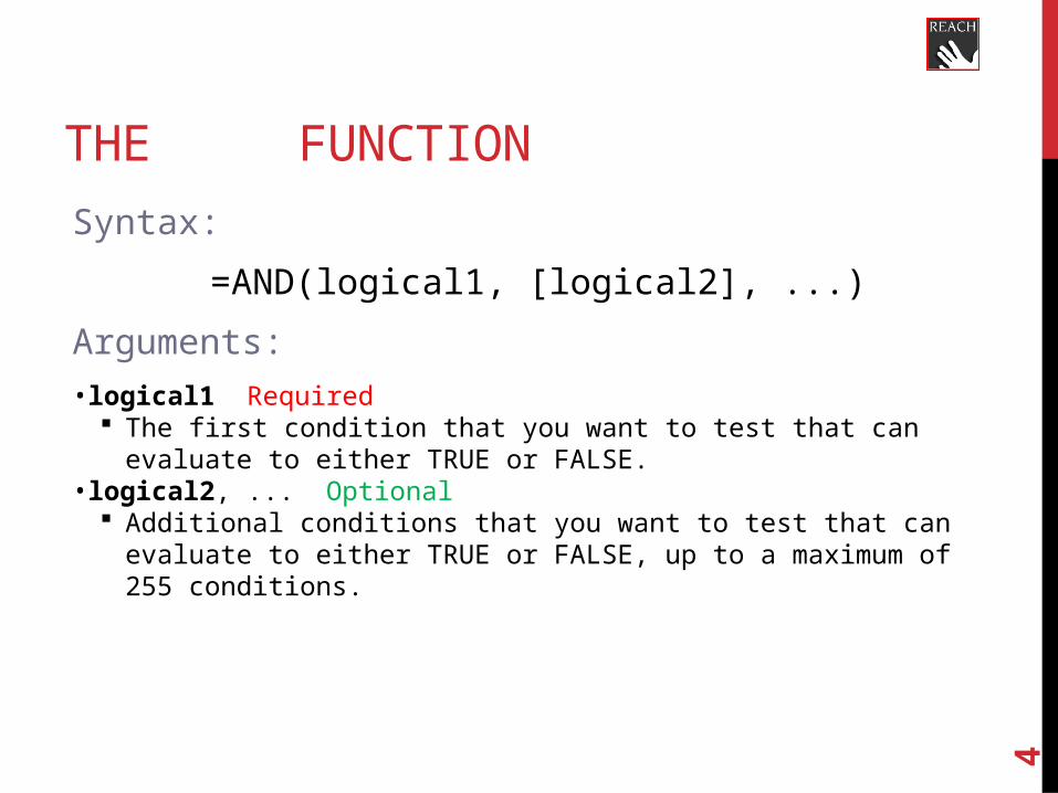
THE AND FUNCTION
Syntax:
=AND(logical1, [logical2], ...)
Arguments:
•logical1 Required The first condition that you want to test that can evaluate to either TRUE or
FALSE.•logical2, ... Optional
Additional conditions that you want to test that can evaluate to either TRUE or FALSE, up to a maximum of 255 conditions.
5
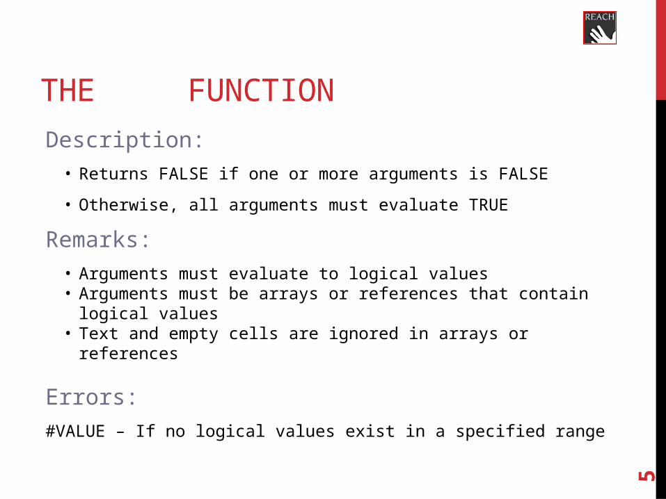
THE AND FUNCTION
Description:
• Returns FALSE if one or more arguments is FALSE
• Otherwise, all arguments must evaluate TRUE
Remarks:
• Arguments must evaluate to logical values• Arguments must be arrays or references that contain logical values• Text and empty cells are ignored in arrays or references
Errors:
#VALUE – If no logical values exist in a specified range
6
THE AND FUNCTION – EXAMPLE 1

7
THE AND FUNCTION – EXAMPLE 2

8
THE OR FUNCTION
Syntax:
=OR(logical1, [logical2], ...)
Arguments:
•logical1 Required The first condition that you want to test that can evaluate to either TRUE or
FALSE.•logical2, ... Optional
Additional conditions that you want to test that can evaluate to either TRUE or FALSE, up to a maximum of 255 conditions.
9
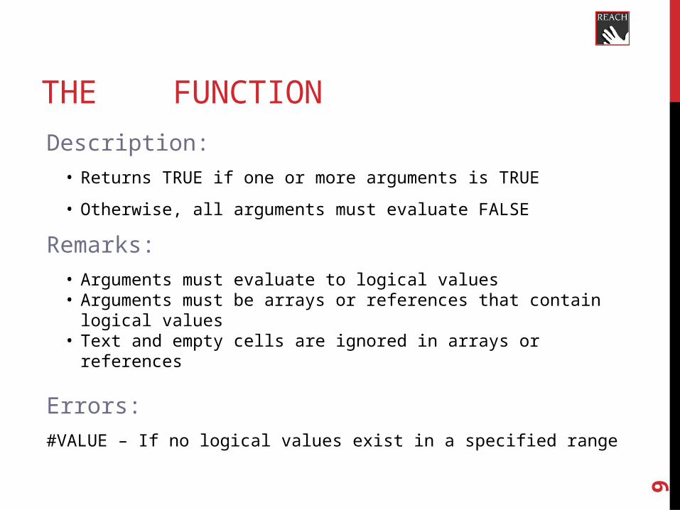
THE OR FUNCTION
Description:
• Returns TRUE if one or more arguments is TRUE
• Otherwise, all arguments must evaluate FALSE
Remarks:
• Arguments must evaluate to logical values• Arguments must be arrays or references that contain logical values• Text and empty cells are ignored in arrays or references
Errors:
#VALUE – If no logical values exist in a specified range

10
THE OR FUNCTION

11
THE NOT FUNCTION
Syntax:
=NOT(logical)
Arguments:
•logical Required A value or expression that can be evaluated to TRUE or FALSE.
12
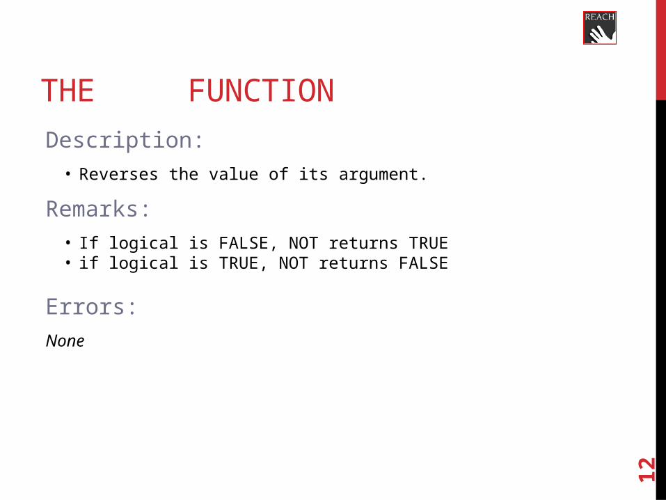
THE NOT FUNCTION
Description:
• Reverses the value of its argument.
Remarks:
• If logical is FALSE, NOT returns TRUE• if logical is TRUE, NOT returns FALSE
Errors:
None

13
THE NOT FUNCTION

14
THE IF FUNCTION
Syntax:
=IF(logical_test, [value_if_true], [value_if_false])
Arguments:
•logical_test Required Any value or expression that can be evaluated to TRUE or FALSE.
•value_if_true Optional• The value that you want to be returned if the logical_test argument
evaluates to TRUE. • If logical_test evaluates to TRUE and the value_if_true argument is omitted
(that is, there is only a comma following the logical_test argument), the IF function returns 0 (zero).
• To display the word TRUE, use the logical value TRUE for the value_if_true argument.

15
THE IF FUNCTION
Syntax:
=IF(logical_test, [value_if_true], [value_if_false])
Arguments:
•value_if_false Optional The value that you want to be returned if the logical_test argument
evaluates to FALSE. If logical_test evaluates to FALSE and the value_if_false argument is
omitted, (that is, there is no comma following the value_if_true argument), the IF function returns the logical value FALSE.
If logical_test evaluates to FALSE and the value of the value_if_false argument is omitted (that is, in the IF function, there is a comma following the value_if_true argument), the IF function returns the value 0 (zero).
16
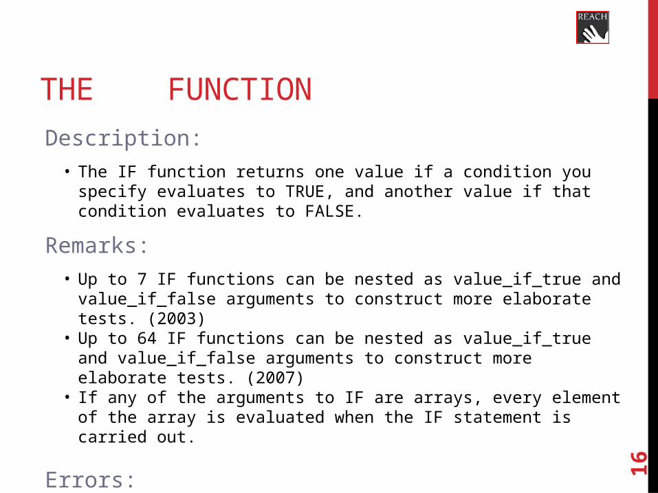
THE IF FUNCTION
Description:
• The IF function returns one value if a condition you specify evaluates to TRUE, and another value if that condition evaluates to FALSE.
Remarks:
• Up to 7 IF functions can be nested as value_if_true and value_if_false arguments to construct more elaborate tests. (2003)
• Up to 64 IF functions can be nested as value_if_true and value_if_false arguments to construct more elaborate tests. (2007)
• If any of the arguments to IF are arrays, every element of the array is evaluated when the IF statement is carried out.
Errors:
None

17
THE IF FUNCTION
value_if_true
[value_if_false]

18
NESTED IF IN EXCEL
http://www.fontstuff.com/excel/exltut01.htm
A nested IF statement says something like...
"If the answer is yes, do this. If the answer is no do this or this (depending on...“
Syntax:
IF( condition1, value_if_true, IF( condition2, value_if_true, value_if_false ))
19
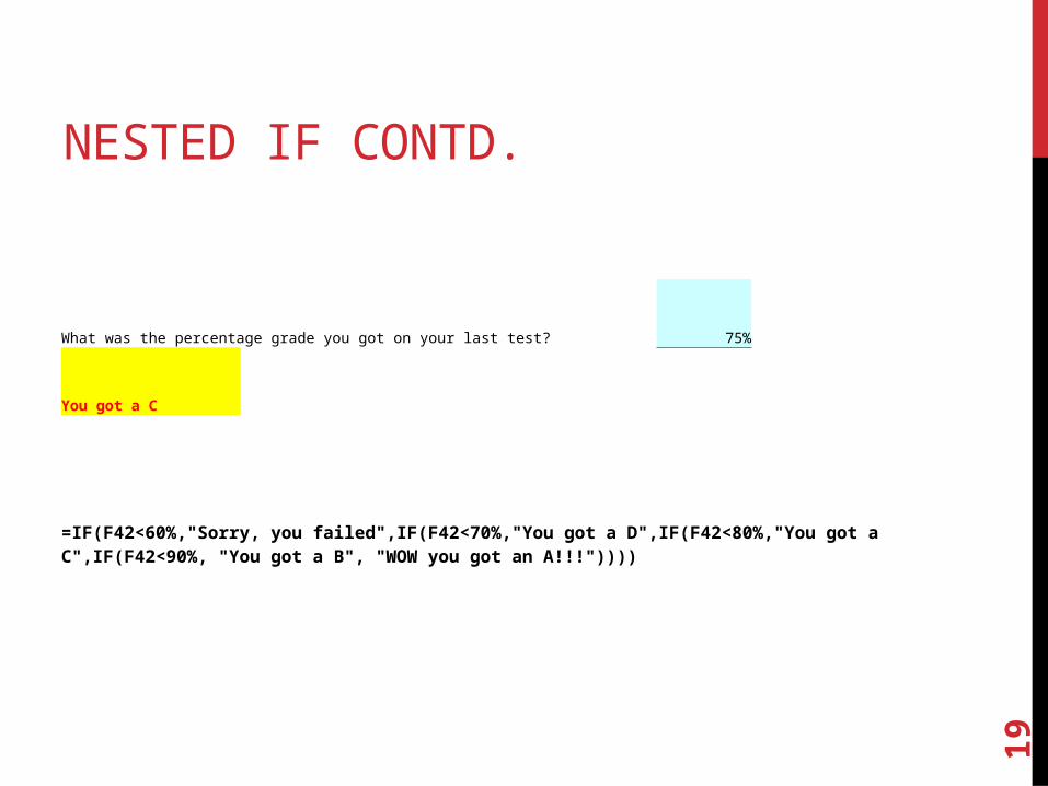
NESTED IF CONTD.
What was the percentage grade you got on your last test? 75%
You got a C
=IF(F42<60%,"Sorry, you failed",IF(F42<70%,"You got a D",IF(F42<80%,"You got a C",IF(F42<90%, "You got a B", "WOW you got an A!!!"))))

20
NESTED IF
Example 2 (Rule 2)
• If cell B1 (which contains a student’s total points out of a 100 scale) is greater than or equal to 90 then give her an A, if it is greater than equal to 80 and less than 90 then give her a B, if it is greater than equal to 70 and less than 80 then give her a C, if it is greater than equal to 60 and less than 70 then give her a D, and if it is less than 60 then give her an F
21
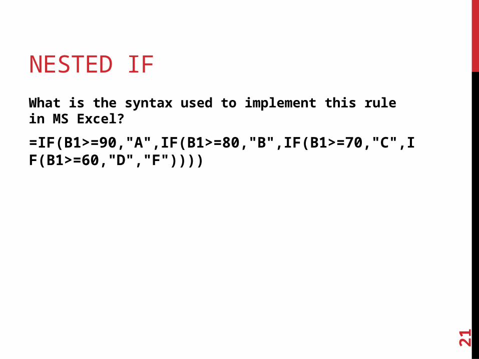
NESTED IF
What is the syntax used to implement this rule in MS Excel?
=IF(B1>=90,"A",IF(B1>=80,"B",IF(B1>=70,"C",IF(B1>=60,"D","F"))))
22
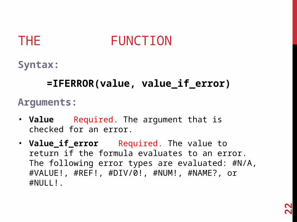
THE IFERROR FUNCTION
Syntax:
=IFERROR(value, value_if_error)
Arguments:
• Value Required. The argument that is checked for an error.
• Value_if_error Required. The value to return if the formula evaluates to an error. The following error types are evaluated: #N/A, #VALUE!, #REF!, #DIV/0!, #NUM!, #NAME?, or #NULL!.
23
THE IFERROR FUNCTION
Description:
• Returns a value you specify if a formula evaluates to an error; otherwise, returns the result of the formula. Use the IFERROR function to trap and handle errors in a formula.
Remarks:
• If value or value_if_error is an empty cell, IFERROR treats it as an empty string value ("").
• If value is an array formula, IFERROR returns an array of results for each cell in the range specified in value. See the second example below.
Errors
• None
24
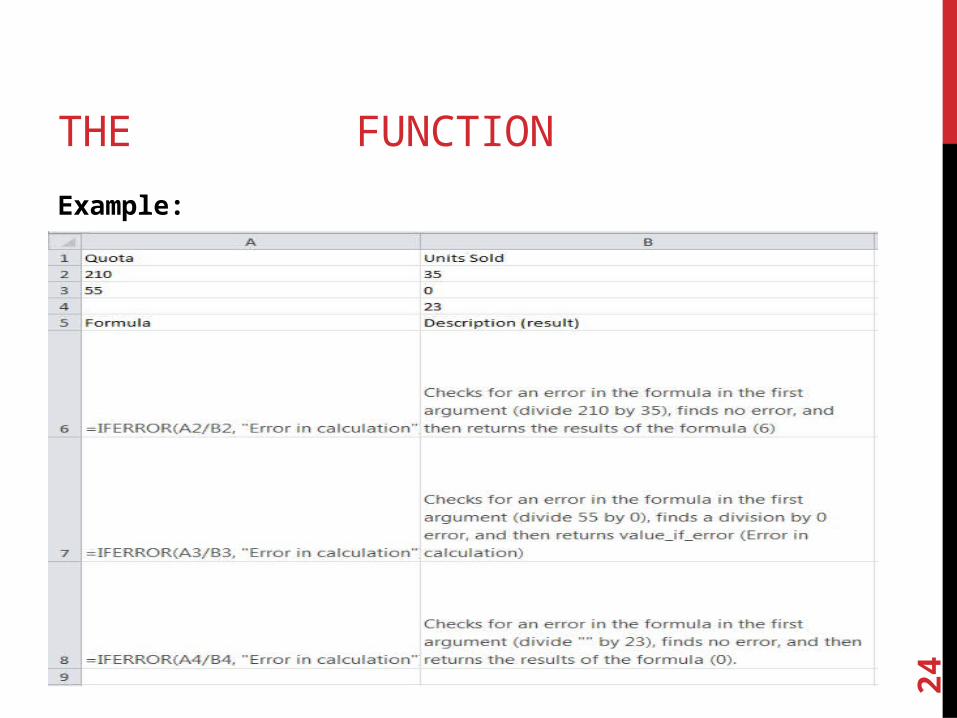
THE IFERROR FUNCTION
Example:

25
Microsoft ExcelMathematical Functions
SUM=SUM(number1,[number2], ...)
SUMIF=SUMIF(range,criteria,[sum_range])
SUMIFS=SUMIFS(sum_range, criteria_range1, criteria1,
[criteria_range2, criteria2], ...)
ROUND=ROUND(number,num_digits)

26
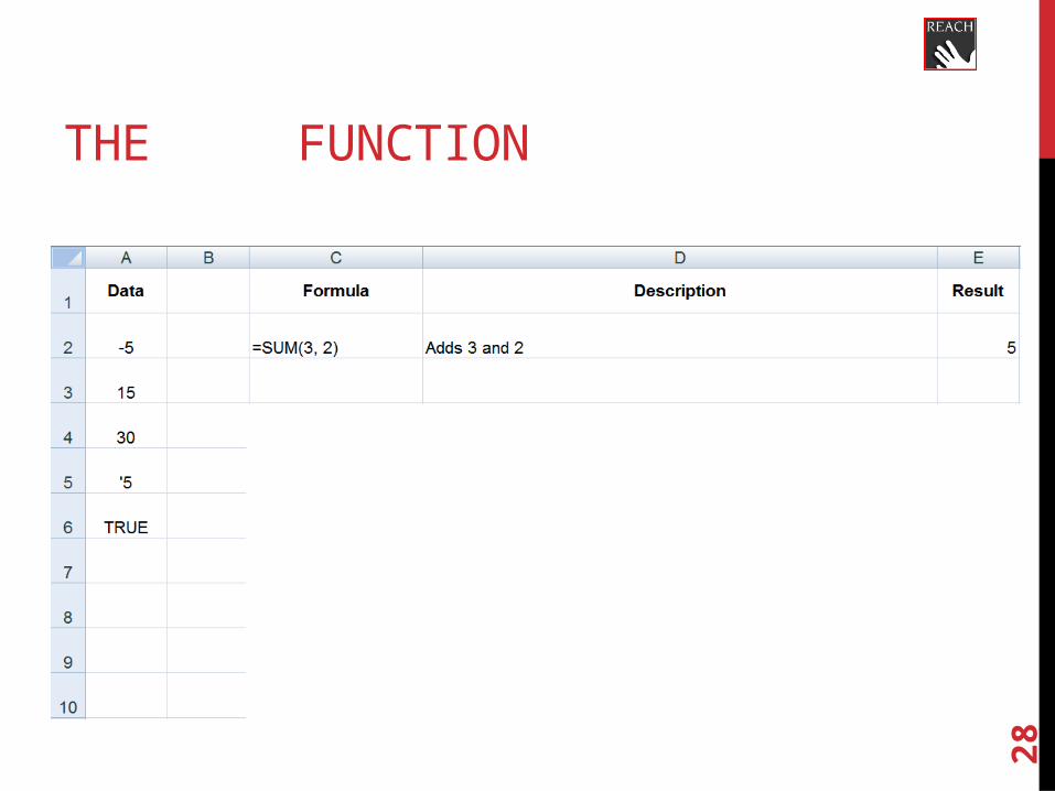
THE SUM FUNCTION
Syntax:
=SUM(number1, [number2], [number3], [number4], ...)
Arguments:
•number1 Required The first item that you want to add.
•number2, number3, number4, ... Optional The remaining items that you want to add, up to a total of 255 items.

27
THE SUM FUNCTION
Description:
• Adds all the numbers that you specify as arguments.
Remarks:
• Each argument can be a range, a cell reference, an array, a constant, a formula, or the result from another function.
• If an argument is an array or reference, only numbers in that array or reference are counted. Empty cells, logical values, or text in the array or reference are ignored.
Errors:
If any arguments are error values, or if any arguments are text that cannot be translated into numbers, Excel displays an error.
28
THE SUM FUNCTION
29
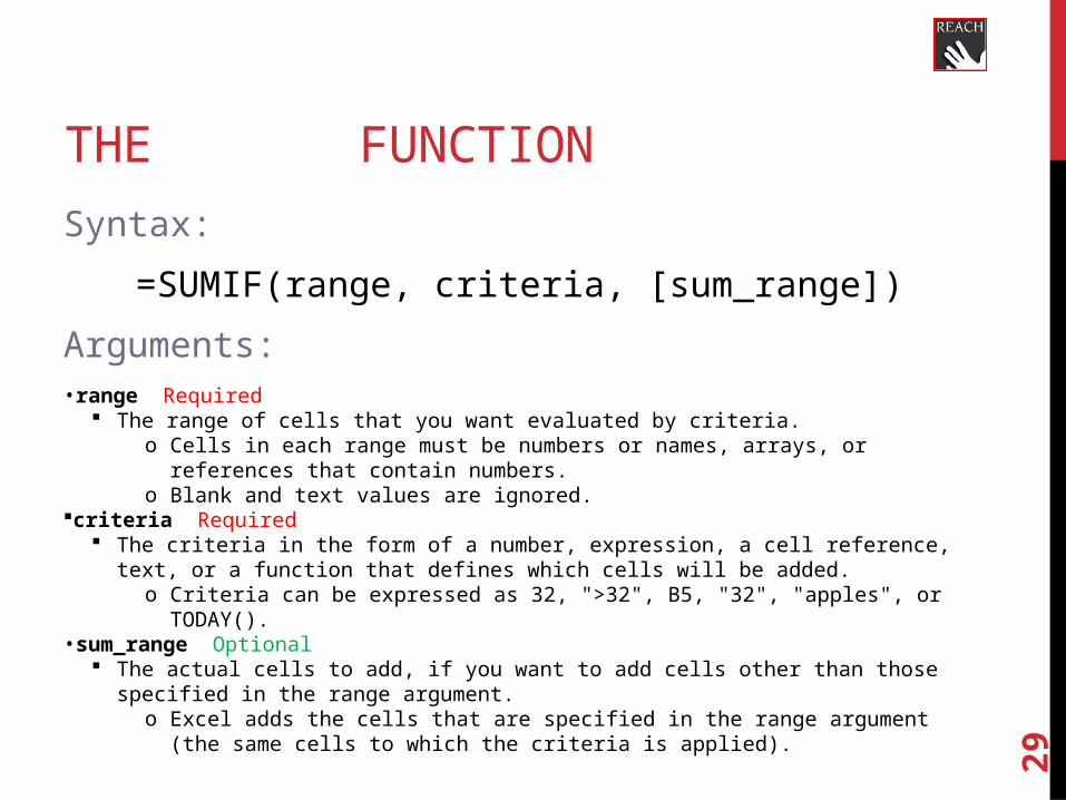
THE SUMIF FUNCTION
Syntax:
=SUMIF(range, criteria, [sum_range])
Arguments:•range Required
The range of cells that you want evaluated by criteria.o Cells in each range must be numbers or names, arrays, or references that contain
numbers.o Blank and text values are ignored.
criteria Required The criteria in the form of a number, expression, a cell reference, text, or a function that
defines which cells will be added.o Criteria can be expressed as 32, ">32", B5, "32", "apples", or TODAY().
•sum_range Optional The actual cells to add, if you want to add cells other than those specified in the range
argument.o Excel adds the cells that are specified in the range argument (the same cells to which
the criteria is applied).

30
THE SUMIF FUNCTION
Description:
• Sums the values in a range that meet criteria that you specify.
Remarks:
• See the Microsoft® Excel® help for additional remarks.
Errors:
None

31
THE SUMIF FUNCTION

32
THE SUMIFS FUNCTION
Syntax:
SUMIFS(sum_range, criteria_range1, criteria1, [criteria_range2, criteria2], ...)
Arguments:
sum_range Required. One or more cells to sum, including numbers or names, ranges, or cell references that contain numbers. Blank and text values are ignored.
criteria_range1 Required. The first range in which to evaluate the associated criteria.
criteria1 Required. The criteria in the form of a number, expression, cell reference, or text that define which cells in the criteria_range1 argument will be added. For example, criteria can be expressed as 32, ">32", B4, "apples", or "32."
criteria_range2, criteria2, … Optional. Additional ranges and their associated criteria. Up to 127 range/criteria pairs are allowed.
33
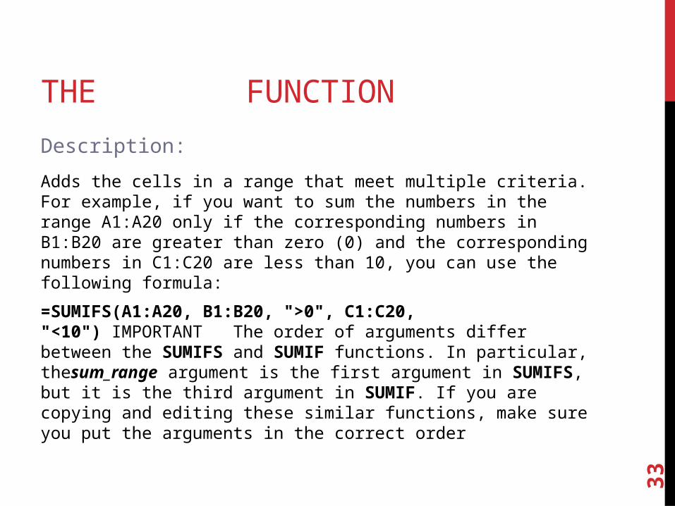
THE SUMIFS FUNCTION
Description:
Adds the cells in a range that meet multiple criteria. For example, if you want to sum the numbers in the range A1:A20 only if the corresponding numbers in B1:B20 are greater than zero (0) and the corresponding numbers in C1:C20 are less than 10, you can use the following formula:
=SUMIFS(A1:A20, B1:B20, ">0", C1:C20, "<10") IMPORTANT The order of arguments differ between the SUMIFS and SUMIF functions. In particular, thesum_range argument is the first argument in SUMIFS, but it is the third argument in SUMIF. If you are copying and editing these similar functions, make sure you put the arguments in the correct order

34
THE SUMIFS FUNCTIONRemarks:
Each cell in the sum_range argument is summed only if all of the corresponding criteria specified are true for that cell. For example, suppose that a formula contains two criteria_range arguments. If the first cell ofcriteria_range1 meets criteria1, and the first cell of criteria_range2 meets critera2, the first cell ofsum_range is added to the sum, and so on, for the remaining cells in the specified ranges.
Cells in the sum_range argument that contain TRUE evaluate to 1; cells in sum_range that contain FALSE evaluate to 0 (zero).
Unlike the range and criteria arguments in the SUMIF function, in the SUMIFS function, each criteria_rangeargument must contain the same number of rows and columns as the sum_range argument.
You can use the wildcard characters — the question mark (?) and asterisk (*) — in criteria. A question mark matches any single character; an asterisk matches any sequence of characters. If you want to find an actual question mark or asterisk, type a tilde (~) before the character.
Errors:
None

35
THE SUMIFS FUNCTION

36
THE ROUND FUNCTION
Syntax:
=ROUND(number, num_digits)
Arguments:
•number Required The number that you want to round.
•num_digits Required The number of digits to which you want to round the number argument.

37
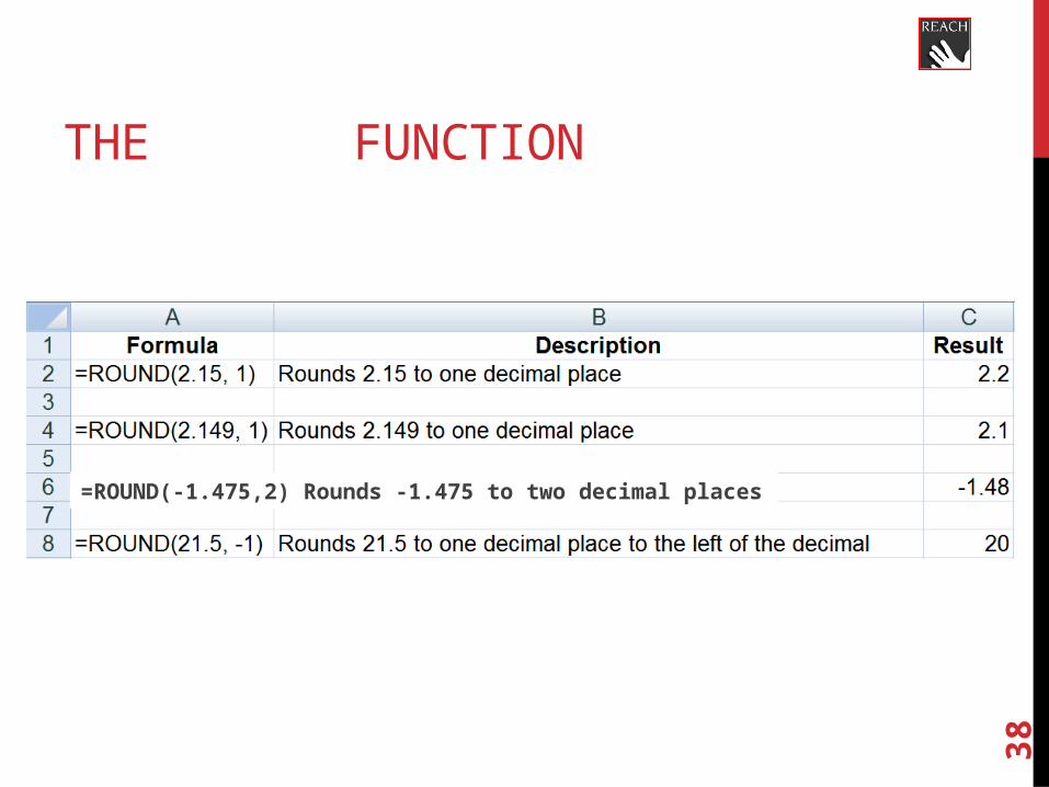
THE ROUND FUNCTION
Description:
• Rounds a number to a specified number of digits.
Remarks:
• If num_digits is greater than 0 (zero), then number is rounded to the specified number of decimal places.
• If num_digits is 0, the number is rounded to the nearest integer. • If num_digits is less than 0, the number is rounded to the left of the decimal
point.
Errors:
None
38
THE ROUND FUNCTION
=ROUND(-1.475,2) Rounds -1.475 to two decimal places

39
MICROSOFT EXCEL
STATISTICAL FUNCTIONSAVERAGE
=AVERAGE(number1, [number2],...)AVERAGEIF
=AVERAGEIF(range, criteria, [average_range])COUNT
=COUNT(value1, [value2],...)COUNTIF
=AVERAGEIF(range, criteria, [average_range])COUNTIFS
COUNTIFS(criteria_range1, criteria1, [criteria_range2, criteria2]…)COUNTA
=COUNTA(value1, [value2],...)MAX
=MAX(number1,[number2],...)MIN
=MIN(number1,[number2],...)LARGE
=LARGE(array,k)SMALL
=LARGE(array,k)

40
THE AVERAGE FUNCTION
Syntax:
=AVERAGE(number1, [number2],...)
Arguments:
•number1 Required The first number, cell reference, or range for which you want the average.
•number2, ... Optional Additional numbers, cell references or ranges for which you want the
average, up to a maximum of 255.

41
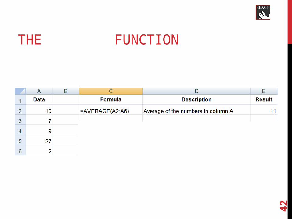
THE AVERAGE FUNCTION
Description:
• Returns the average (arithmetic mean) of the arguments.
Remarks:• Arguments can either be numbers or names, ranges, or cell references that contain
numbers.• Logical values and text representations of numbers that you type directly into the list
of arguments are counted.• If a range or cell reference argument contains text, logical values, or empty cells,
those values are ignored; however, cells with the value zero are included.
Errors:
Arguments that are error values or text that cannot be translated into numbers cause errors.
42
THE AVERAGE FUNCTION
43
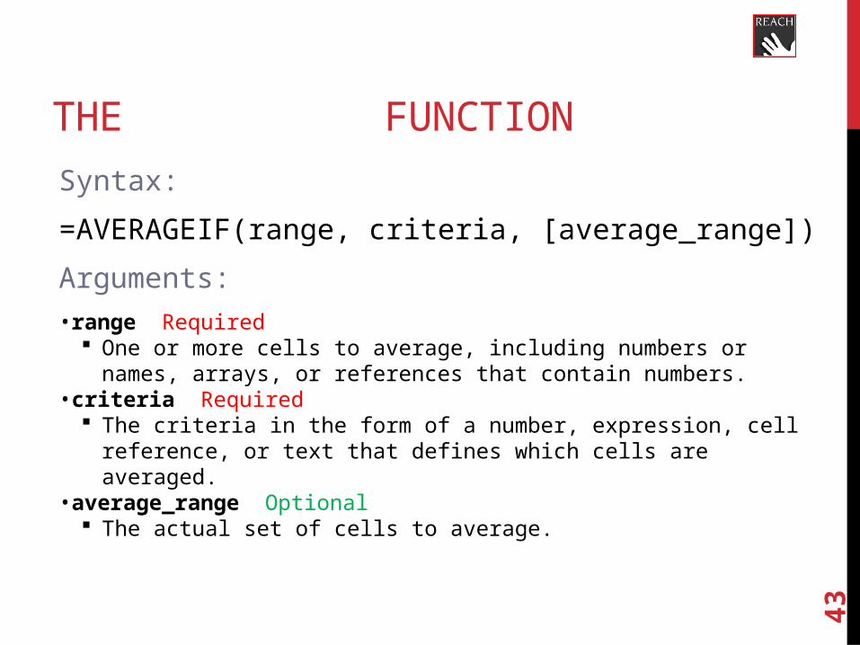
THE AVERAGEIF FUNCTION
Syntax:
=AVERAGEIF(range, criteria, [average_range])
Arguments:
•range Required One or more cells to average, including numbers or names, arrays, or
references that contain numbers.•criteria Required
The criteria in the form of a number, expression, cell reference, or text that defines which cells are averaged.
•average_range Optional The actual set of cells to average.

44
THE AVERAGEIF FUNCTION
Description:
• Returns the average (arithmetic mean) of all the cells in a range that meet a given criteria.
Remarks:• If average_range is omitted, range is used.• Cells in range that contain TRUE or FALSE are ignored.• If a cell in average_range is an empty cell, AVERAGEIF ignores it.• If a cell in criteria is empty, AVERAGEIF treats it as a 0 value.
Errors:
#DIV/0 – If range is a blank or text value.
#DIV/0 – If no cells in the range meet the criteria.
45
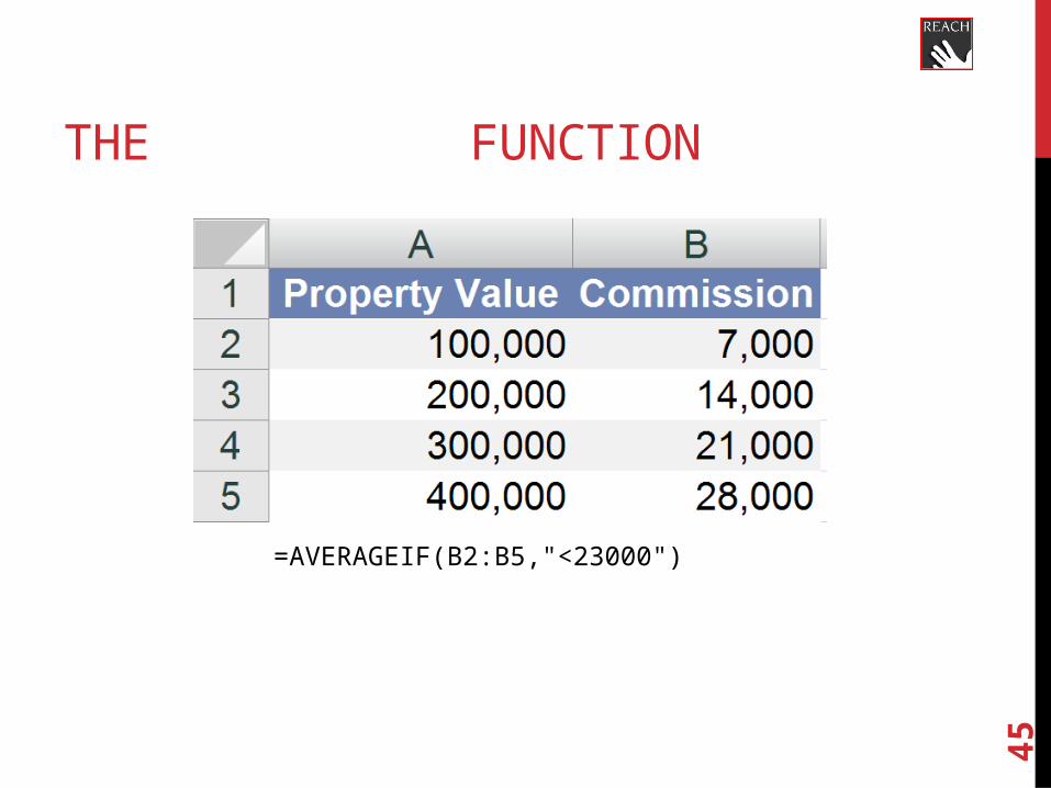
THE AVERAGEIF FUNCTION
=AVERAGEIF(B2:B5,"<23000")
46
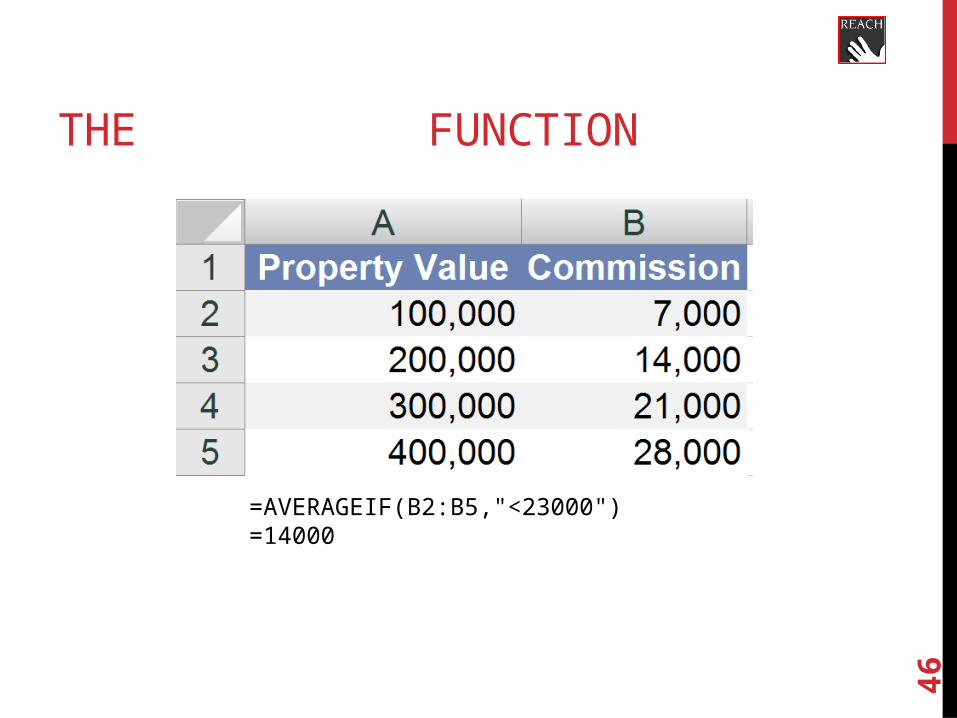
THE AVERAGEIF FUNCTION
=AVERAGEIF(B2:B5,"<23000")=14000

47
THE AVERAGEIF FUNCTION
=AVERAGEIF(A2:A5,"<95000")

48
THE AVERAGEIF FUNCTION
=AVERAGEIF(A2:A5,"<95000")=#DIV/0

49
THE AVERAGEIF FUNCTION
=AVERAGEIF(A2:A5,">250000",B2:B5)

50
THE AVERAGEIF FUNCTION
=AVERAGEIF(A2:A5,">250000",B2:B5)=24500

51
THE AVERAGEIFS FUNCTION
Syntax:
AVERAGEIFS(average_range, criteria_range1, criteria1, [criteria_range2, criteria2], ...)
Arguments:
•Average_range Required. One or more cells to average, including numbers or names, arrays, or references that contain numbers.•Criteria_range1, criteria_range2, … Criteria_range1 is required, subsequent criteria_ranges are optional. 1 to 127 ranges in which to evaluate the associated criteria.•Criteria1, criteria2, ... Criteria1 is required, subsequent criteria are optional. 1 to 127 criteria in the form of a number, expression, cell reference, or text that define which cells will be averaged. For example, criteria can be expressed as 32, "32", ">32", "apples", or B4.

52
THE AVERAGEIFS FUNCTION
Description:•Returns the average (arithmetic mean) of all cells that meet multiple criteria.
Remarks:
• If average_range is a blank or text value, AVERAGEIFS returns the #DIV0! error value.
• If a cell in a criteria range is empty, AVERAGEIFS treats it as a 0 value.
• Cells in range that contain TRUE evaluate as 1; cells in range that contain FALSE evaluate as 0 (zero).
• Each cell in average_range is used in the average calculation only if all of the corresponding criteria specified are true for that cell.
• Unlike the range and criteria arguments in the AVERAGEIF function, in AVERAGEIFS each criteria_range must be the same size and shape as sum_range.
• If cells in average_range cannot be translated into numbers, AVERAGEIFS returns the #DIV0! error value.
• If there are no cells that meet all the criteria, AVERAGEIFS returns the #DIV/0! error value.
• You can use the wildcard characters, question mark (?) and asterisk (*), in criteria. A question mark matches any single character; an asterisk matches any sequence of characters. If you want to find an actual question mark or asterisk, type a tilde (~) before the character.
Errors:
None.
53
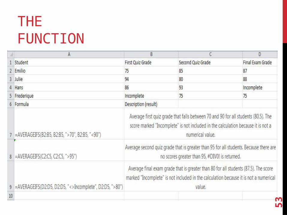
THE AVERAGEIFS FUNCTION
54
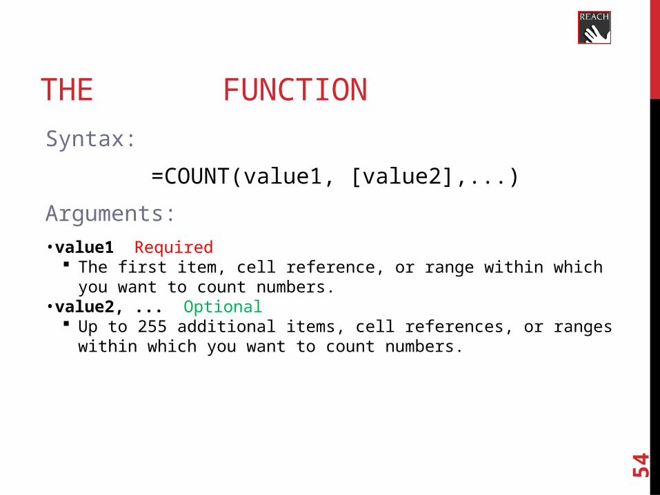
THE COUNT FUNCTION
Syntax:
=COUNT(value1, [value2],...)
Arguments:
•value1 Required The first item, cell reference, or range within which you want to count
numbers.•value2, ... Optional
Up to 255 additional items, cell references, or ranges within which you want to count numbers.
55
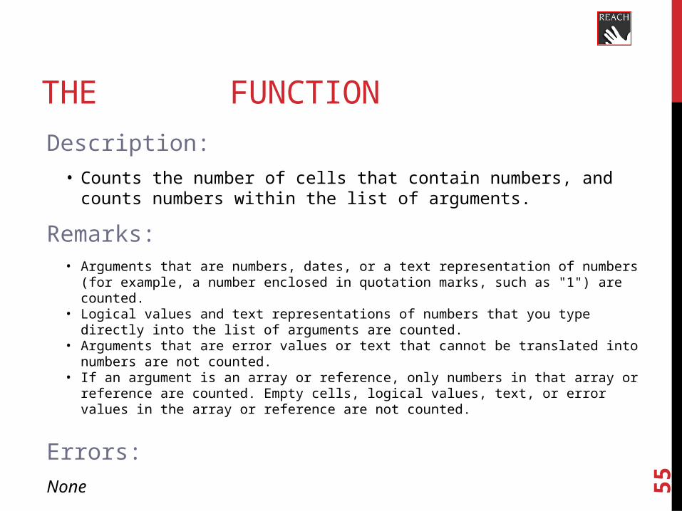
THE COUNT FUNCTION
Description:
• Counts the number of cells that contain numbers, and counts numbers within the list of arguments.
Remarks:• Arguments that are numbers, dates, or a text representation of numbers (for example, a number
enclosed in quotation marks, such as "1") are counted.• Logical values and text representations of numbers that you type directly into the list of
arguments are counted.• Arguments that are error values or text that cannot be translated into numbers are not counted. • If an argument is an array or reference, only numbers in that array or reference are counted.
Empty cells, logical values, text, or error values in the array or reference are not counted.
Errors:
None

56
THE COUNT FUNCTION
57
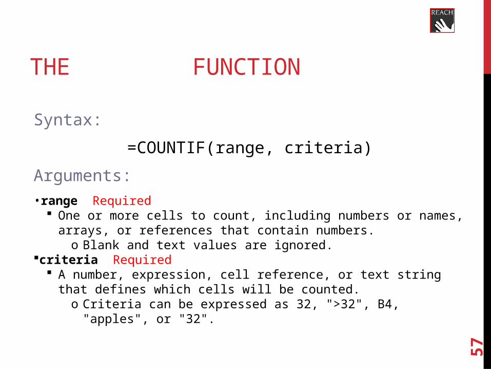
THE COUNTIF FUNCTION
Syntax:
=COUNTIF(range, criteria)
Arguments:
•range Required One or more cells to count, including numbers or names, arrays, or
references that contain numbers.o Blank and text values are ignored.
criteria Required A number, expression, cell reference, or text string that defines which cells
will be counted.o Criteria can be expressed as 32, ">32", B4, "apples", or "32".
58
THE COUNTIF FUNCTION
Description:
• Counts the number of cells within a range that meet a single criterion that you specify.
Remarks:• See the Microsoft® Excel® help for additional remarks.• Criteria are case insensitive
Errors:
None
59
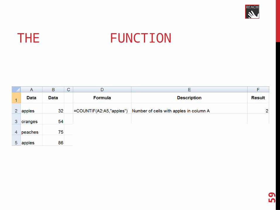
THE COUNTIF FUNCTION

60
THE COUNTIFS FUNCTIONSyntax:
COUNTIFS(criteria_range1, criteria1, [criteria_range2, criteria2]…)
Arguments:
• criteria_range1 Required. The first range in which to evaluate the associated criteria.
• criteria1 Required. The criteria in the form of a number, expression, cell reference, or text that define which cells will be counted. For example, criteria can be expressed as 32, ">32", B4, "apples", or "32".
• criteria_range2, criteria2, ... Optional. Additional ranges and their associated criteria. Up to 127 range/criteria pairs are allowed.
IMPORTANT Each additional range must have the same number of rows and columns as the criteria_range1argument. The ranges do not have to be adjacent to each other.

61
THE COUNTIFS FUNCTION
Description:
• Applies criteria to cells across multiple ranges and counts the number of times all criteria are met.
Remarks:
Each range's criteria is applied one cell at a time. If all of the first cells meet their associated criteria, the count increases by 1. If all of the second cells meet their associated criteria, the count increases by 1 again, and so on until all of the cells are evaluated.If the criteria argument is a reference to an empty cell, the COUNTIFS function treats the empty cell as a 0 value.You can use the wildcard characters— the question mark (?) and asterisk (*) — in criteria. A question mark matches any single character, and an asterisk matches any sequence of characters. If you want to find an actual question mark or asterisk, type a tilde (~) before the character.
Errors:
None

62
THE COUNTIFS FUNCTION
63
THE COUNTA FUNCTION
Syntax:
=COUNTA(value1, [value2],...)
Arguments:
•value1 Required The first argument representing the values that you want to count.
•value2, ... Optional Additional arguments representing the values that you want to count, up to
a maximum of 255 arguments.

64
THE COUNTA FUNCTION
Description:
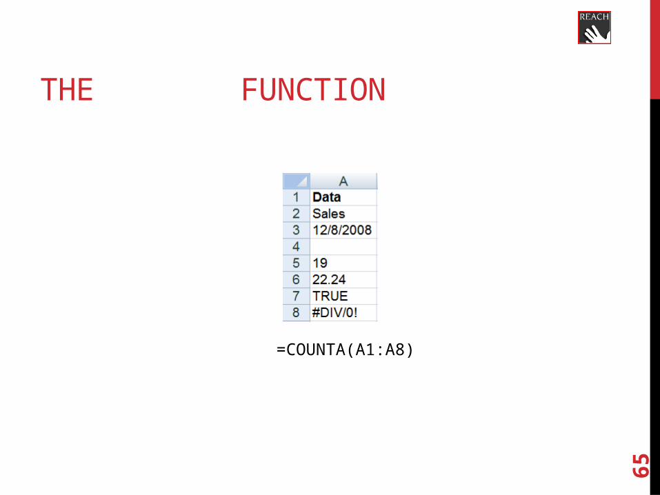
• Counts the number of cells that are not empty in a range.
Remarks:
• Counts cells containing any type of information, including error values and empty text ("“).
• The COUNTA function does not count empty cells.
Errors:
None
65
THE COUNTA FUNCTION
=COUNTA(A1:A8)
66
THE MAX FUNCTION
Syntax:
=MAX(number1,[number2],...)
Arguments:
•number1, number2, ... Required 1 to 255 numbers for which you want to find the maximum value.

67
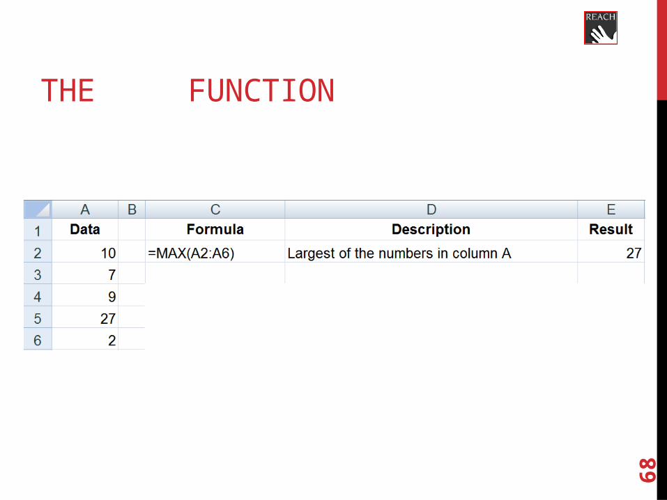
THE MAX FUNCTION
Description:
• Returns the largest value in a set of values.
Remarks:• Arguments can either be numbers or names, arrays, or references that contain
numbers. • Logical values and text representations of numbers that you type directly into the list
of arguments are counted. • If an argument is an array or reference, only numbers in that array or reference are
used. Empty cells, logical values, or text in the array or reference are ignored.• If the arguments contain no numbers, MAX returns 0 (zero).
Errors:
Arguments that are error values or text that cannot be translated into numbers cause errors.
68
THE MAX FUNCTION

69
THE MIN FUNCTION
Syntax:
=MIN(number1,[number2],...)
Arguments:
•number1, number2, ... Required 1 to 255 numbers for which you want to find the minimum value.
70
THE MIN FUNCTION
Description:
• Returns the smallest value in a set of values.
Remarks:• Arguments can either be numbers or names, arrays, or references that contain
numbers. • Logical values and text representations of numbers that you type directly into the list
of arguments are counted. • If an argument is an array or reference, only numbers in that array or reference are
used. Empty cells, logical values, or text in the array or reference are ignored.• If the arguments contain no numbers, MIN returns 0 (zero).
Errors:
Arguments that are error values or text that cannot be translated into numbers cause errors.

71
THE MIN FUNCTION
72
THE LARGE FUNCTION
Syntax:
=LARGE(array,k)
Arguments:
•array Required The array or range of data for which you want to determine the k-th largest
value.k Required
The position (from the largest) in the array or cell range of data to return.

73
THE LARGE FUNCTION
Description:
• Returns the k-th largest value in a data set.
Remarks:• If n is the number of data points in a range, then LARGE(array,1) returns the largest
value.• If n is the number of data points in a range, then LARGE(array,n) returns the
smallest value.
Errors:
#NUM! – If array is empty#NUM! – If k ≤ 0#NUM! – If k is greater than the number of data points

74
=LARGE(array,k)
3rd largest number in the numbers in columns A and B

75
=LARGE(array,k)=LARGE(A2:B6
3rd largest number in the numbers in columns A and B

76
=LARGE(array,k)=LARGE(A2:B6,3)
3rd largest number in the numbers in columns A and B
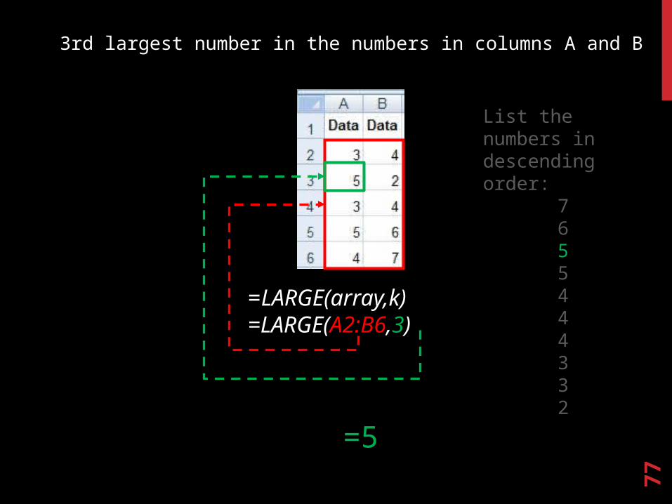
77
=LARGE(array,k)=LARGE(A2:B6,3)
3rd largest number in the numbers in columns A and B
List the numbers in descending order:
7655444332
=5

78
=LARGE(array,k)
7th largest number in the numbers in columns A and B
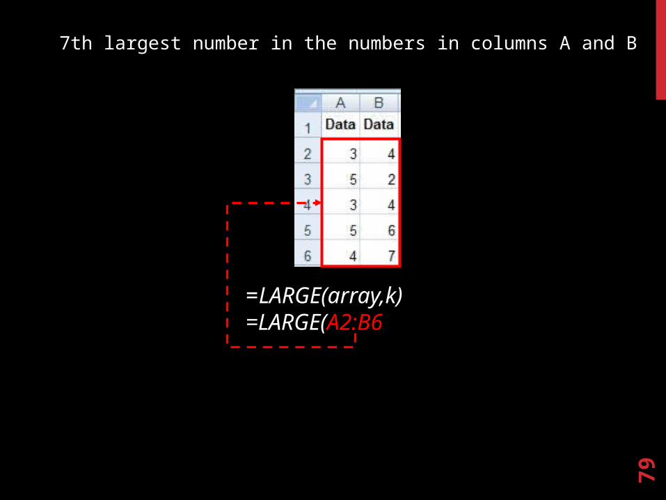
79
=LARGE(array,k)=LARGE(A2:B6
7th largest number in the numbers in columns A and B

80
=LARGE(array,k)=LARGE(A2:B6,7)
7th largest number in the numbers in columns A and B

81
=LARGE(array,k)=LARGE(A2:B6,7)
7th largest number in the numbers in columns A and B
List the numbers in descending order:
7655444332

82
=LARGE(array,k)=LARGE(A2:B6,7)
7th largest number in the numbers in columns A and B
List the numbers in descending order:
7655444332
=4

83
THE SMALL FUNCTION
Syntax:
=SMALL(array,k)
Arguments:
•array Required The array or range of data for which you want to determine the k-th
smallest value.k Required
The position (from the smallest) in the array or cell range of data to return.

84
THE SMALL FUNCTION
Description:
• Returns the k-th smallest value in a data set.
Remarks:• If n is the number of data points in a range, then SMALL(array,1) returns the
smallest value.• If n is the number of data points in a range, then SMALL(array,n) returns the largest
value.
Errors:
#NUM! – If array is empty#NUM! – If k ≤ 0#NUM! – If k is greater than the number of data points
85
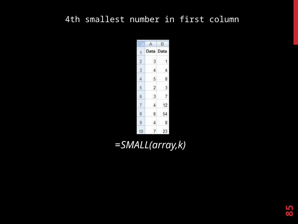
=SMALL(array,k)
4th smallest number in first column

86
=SMALL(array,k)=SMALL(A2:A10
4th smallest number in first column

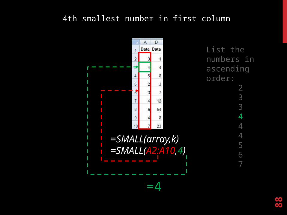
87
=SMALL(array,k)=SMALL(A2:A10,4)
4th smallest number in first column
List the numbers in ascending order:
233444567
88
=SMALL(array,k)=SMALL(A2:A10,4)
4th smallest number in first column
List the numbers in ascending order:
233444567
=4

89
=SMALL(array,k)
2nd smallest number in second column

90
=SMALL(array,k)=SMALL(B2:B10
2nd smallest number in second column

91
=SMALL(array,k)=SMALL(B2:B10,2)
2nd smallest number in second column
List the numbers in ascending order:
134788
122354

92
=SMALL(array,k)=SMALL(B2:B10,2)
2nd smallest number in second column
=3
List the numbers in ascending order:
134788
122354

93
MICROSOFT EXCEL LOOKUP FUNCTIONS
VLOOKUP=VLOOKUP(lookup_value, table_array, col_index_num,
[range_lookup])HLOOKUP
= HLOOKUP(lookup_value,table_array,row_index_num,range_lookup)

94
THE VLOOKUP FUNCTION
Syntax:
=VLOOKUP(lookup_value,table_array,col_index_num,[range_lookup])
Arguments:
•lookup_value Required The value to search in the first column of the table or range.
•table_array Required The range of cells that contains the data.
•col_index_num Required The column number in the table_array argument from which the matching
value must be returned. •range_lookup Optional
A logical value that specifies whether you want VLOOKUP to find an exact match or an approximate match.
95
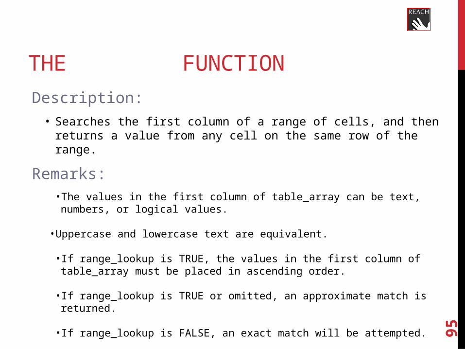
THE VLOOKUP FUNCTION
Description:
• Searches the first column of a range of cells, and then returns a value from any cell on the same row of the range.
Remarks:• The values in the first column of table_array can be text, numbers, or logical
values.
• Uppercase and lowercase text are equivalent.
• If range_lookup is TRUE, the values in the first column of table_array must be placed in ascending order.
• If range_lookup is TRUE or omitted, an approximate match is returned.
• If range_lookup is FALSE, an exact match will be attempted.
96
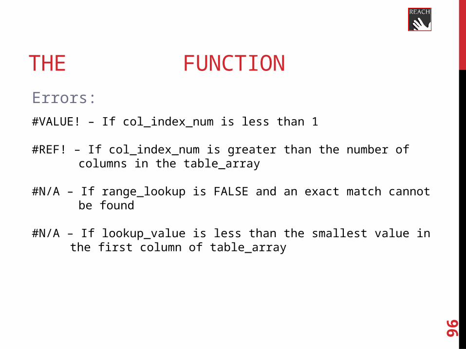
THE VLOOKUP FUNCTION
Errors:
#VALUE! – If col_index_num is less than 1
#REF! – If col_index_num is greater than the number of columns in the table_array
#N/A – If range_lookup is FALSE and an exact match cannot be found
#N/A – If lookup_value is less than the smallest value in the first column of table_array

97
(1) =VLOOKUP(C11*2, $B$8:$G$24, G18/E6, TRUE)
98
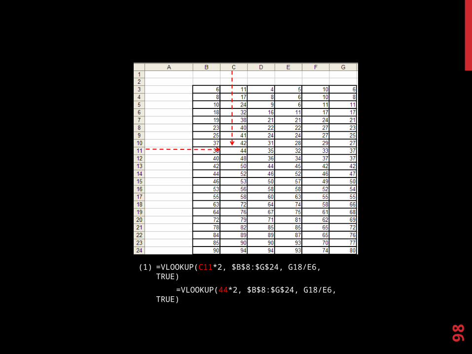
(1) =VLOOKUP(C11*2, $B$8:$G$24, G18/E6, TRUE)
=VLOOKUP(44*2, $B$8:$G$24, G18/E6, TRUE)

99
(1) =VLOOKUP(C11*2, $B$8:$G$24, G18/E6, TRUE)
=VLOOKUP(44*2, $B$8:$G$24, G18/E6, TRUE)
=VLOOKUP(88, $B$8:$G$24, G18/E6, TRUE)

100
(1) =VLOOKUP(C11*2, $B$8:$G$24, G18/E6, TRUE)
=VLOOKUP(44*2, $B$8:$G$24, G18/E6, TRUE)
=VLOOKUP(88, $B$8:$G$24, G18/E6, TRUE)

101
(1) =VLOOKUP(C11*2, $B$8:$G$24, G18/E6, TRUE)
=VLOOKUP(44*2, $B$8:$G$24, G18/E6, TRUE)
=VLOOKUP(88, $B$8:$G$24, G18/E6, TRUE)
=VLOOKUP(88, $B$8:$G$24, 66/E6, TRUE)

102
(1) =VLOOKUP(C11*2, $B$8:$G$24, G18/E6, TRUE)
=VLOOKUP(44*2, $B$8:$G$24, G18/E6, TRUE)
=VLOOKUP(88, $B$8:$G$24, G18/E6, TRUE)
=VLOOKUP(88, $B$8:$G$24, 66/E6, TRUE)
=VLOOKUP(88, $B$8:$G$24, 66/11, TRUE)
103
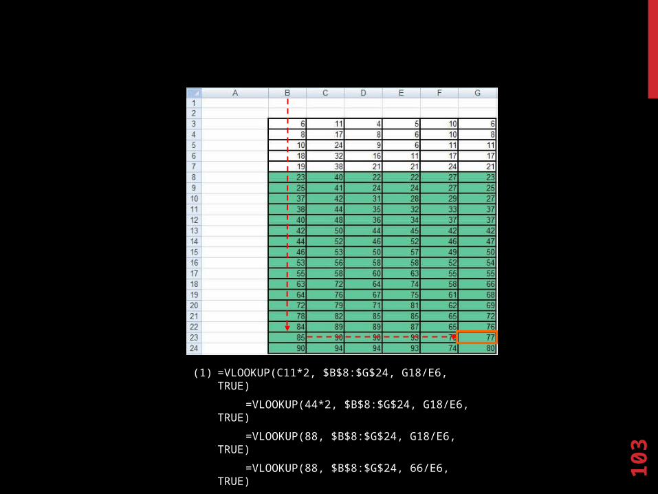
(1) =VLOOKUP(C11*2, $B$8:$G$24, G18/E6, TRUE)
=VLOOKUP(44*2, $B$8:$G$24, G18/E6, TRUE)
=VLOOKUP(88, $B$8:$G$24, G18/E6, TRUE)
=VLOOKUP(88, $B$8:$G$24, 66/E6, TRUE)
=VLOOKUP(88, $B$8:$G$24, 66/11, TRUE)
=VLOOKUP(88, $B$8:$G$24, 6, TRUE)
104
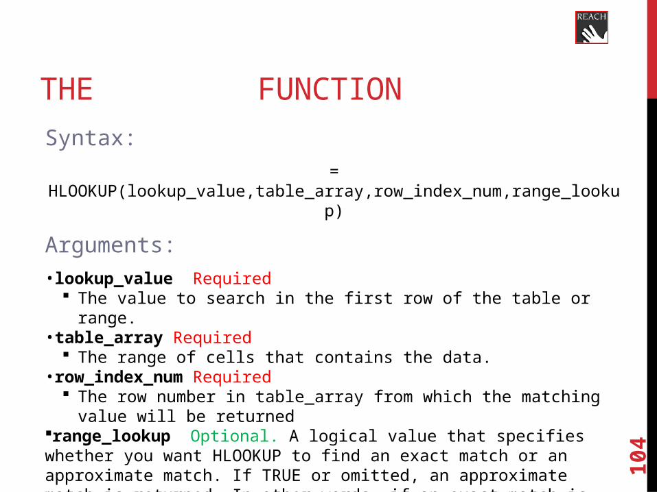
THE HLOOKUP FUNCTION
Syntax:
= HLOOKUP(lookup_value,table_array,row_index_num,range_lookup)
Arguments:
•lookup_value Required The value to search in the first row of the table or range.
•table_array Required The range of cells that contains the data.
•row_index_num Required The row number in table_array from which the matching value will be
returned range_lookup Optional. A logical value that specifies whether you want HLOOKUP to find an exact match or an approximate match. If TRUE or omitted, an approximate match is returned. In other words, if an exact match is not found, the next largest value that is less than lookup_value is returned. If FALSE, HLOOKUP will find an exact match. If one is not found, the error value #N/A is returned.

105
THE HLOOKUP FUNCTIONDescription:
• Searches for a value in the top row of a table or an array of values, and then returns a value in the same column from a row you specify in the table or array.
Remarks:
• If HLOOKUP can't find lookup_value, and range_lookup is TRUE, it uses the largest value that is less than lookup_value.
• If lookup_value is smaller than the smallest value in the first row of table_array, HLOOKUP returns the #N/A error value.

106
THE HLOOKUP FUNCTION
Errors:
#VALUE! – If row_index_num is less than 1
#REF! – If row_index_num is greater than the number of rows in the table_array
#N/A – If range_lookup is FALSE and an exact match cannot be found
#N/A – If lookup_value is less than the smallest value in the first row of table_array
107
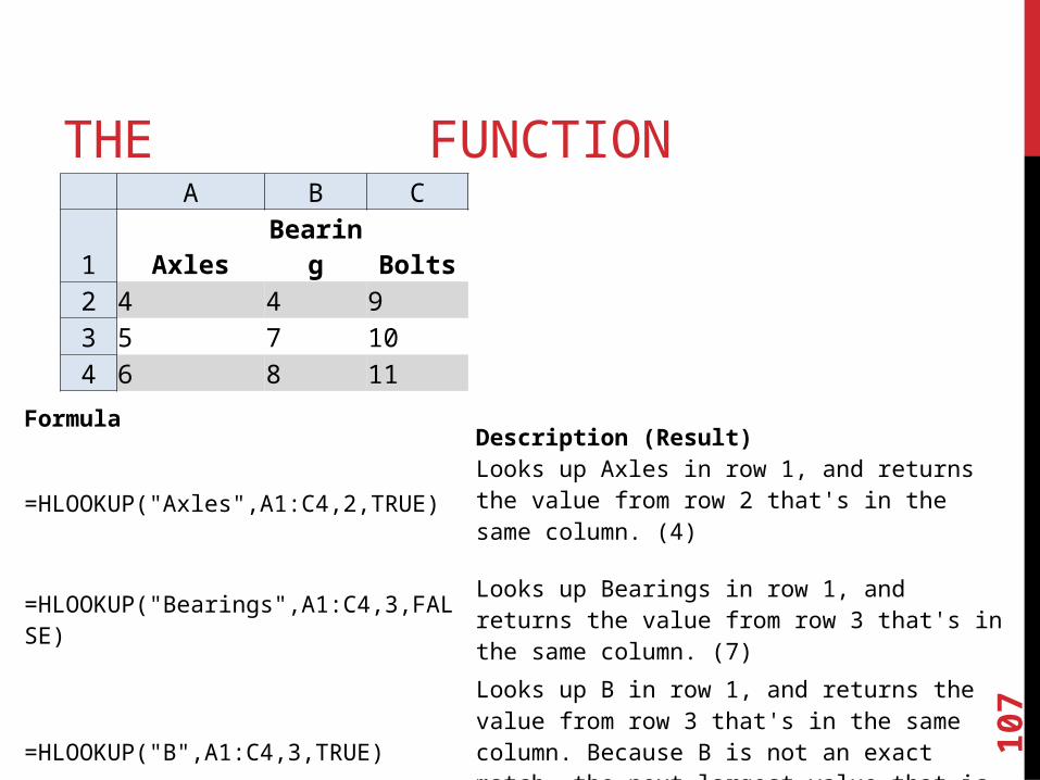
THE HLOOKUP FUNCTION A B C1 Axles Bearing Bolts2 4 4 93 5 7 104 6 8 11
FormulaDescription (Result)Looks up Axles in row 1, and returns the value from row 2 that's in the same column. (4)=HLOOKUP("Axles",A1:C4,2,TRUE)
=HLOOKUP("Bearings",A1:C4,3,FALSE) Looks up Bearings in row 1, and returns the value from row 3 that's in the same column. (7)
=HLOOKUP("B",A1:C4,3,TRUE)
Looks up B in row 1, and returns the value from row 3 that's in the same column. Because B is not an exact match, the next largest value that is less than B is used: Axles. (5)
=HLOOKUP("Bolts",A1:C4,4) Looks up Bolts in row 1, and returns the value from row 4 that's in the same column. (11)

108
The worksheet above lists the annual salaries for a company’s employees. (A) What is the formula to determine the total number of employees who earn
between $50,000 and $70,000 in annual salary (inclusive)? =COUNTIFS(C4:C14,">50000",C4:C14,"<70000")
(B) What is the formula to determine the sum of the salaries of employees who have first names that begin with the letter A?
=SUMIFS(C4:C14,B4:B14,"=A*") (C) What is the formula to determine the average salary of employees who earn more than the third (3rd) highest salary?
=AVERAGEIF(C4:C14,">"&LARGE(C4:C14,3),C4:C14)

109

110


