"J CITIDMSP - citibank's Direct Marketing Software Package Akos Felsovcilyi, citibank ABSTRACT The paper introduces CITIDMSP, citibank's SAS-base program package for direct marketing applications. The key system activities of quantitative direct marketing are testing, profiling the responders, building statistical models for predicting response, scoring the customer base with a response model and finally; segmenting the customer base for a profitable solicitation. The package offers all system and statistical tools to automate and to standardize all these activities. The package is written in the SAS macro language and it provides an easy, flexible, single-environment solution for systems applications in direct marketing. The paper describes the package and then demonstrates its main features by applying it to a fictitious direct marketing program. INTRODUCTION Direct marketing has many definitions. According to one of them {9}: !I Direct (response) marketing is the total of activities by which products and services are ,offered to market segments in one or more media for informational purposes, or to solicit a direct response from a present or prospective customer or contributor by mail, telephone or other access. 1I Let us define some terms of direct marketing we will refer to in this paper. Direct Marketing Campaigh: a mail, telemarketing (or other type of) solicitation that offers a product or service to customers chosen for the campaign. Test Campaign: a direct marketing campaign to a representative sample of a population with the aim of testing a product and/or developing segmentation models. Response Profile: the common characteristics of the responders relative to all customers solicit""ted .in a direct marketing campaign. Response Model: a statistical model (derived from the response profile) to predict the likelihood of response of every customer of a population. Scoring: application ofa response model to a pOPUla:tion, that is, calculating the response probability Of its every customer based on the response model. Segmentation: partition of a population into segments of different response probabilities based on the scores of its members. A future campaign attempts to target profitable segments. Although direct marketing relies on many other activities (for example, choosing the right medium, phrasing and packaging the offer, etc.), this paper will focus on its system-related activities only. The terms defined above describe the most significant system-related steps a direct marketer has to take: testing, profiling the responders, developing response models, scoring the population and finally segmenting it for a future campaign. Because of its vast quantities of data and the paramount importance of segmentation, direct marketing has been associated with and. depending on computer processing and mathematical statistics. Due to this double requirement, the SAS System \ ideally lends itself to.direct marketing. Its· data processing power and the whole \; spectrum of its statistical it the numberonechoicefor.thetask. 47
Transcript
"J
CITIDMSP - citibank's Direct Marketing Software Package
Akos Felsovcilyi, citibank
ABSTRACT
The paper introduces CITIDMSP, citibank's SAS-base program package for direct marketing applications.
The key system activities of quantitative direct marketing are testing, profiling the responders, building statistical models for predicting response, scoring the customer base with a response model and finally; segmenting the customer base for a profitable solicitation. The package offers all system and statistical tools to automate and to standardize all these activities.
The package is written in the SAS macro language and it provides an easy, flexible, single-environment solution for systems applications in direct marketing.
The paper describes the package and then demonstrates its main features by applying it to a fictitious direct marketing program.
INTRODUCTION
Direct marketing has many definitions. According to one of them {9}: !I Direct (response) marketing is the total of activities by which products and services are
,offered to market segments in one or more media for informational purposes, or to solicit a direct response from a present or prospective customer or contributor by mail, telephone or other access. 1I Let us define some terms of direct marketing we will refer to in this paper.
Direct Marketing Campaigh: a mail, telemarketing (or other type of) solicitation that offers a product or service to customers chosen for the campaign.
Test Campaign: a direct marketing campaign to a representative sample of a population with the aim of testing a product and/or developing segmentation models.
Response Profile: the common characteristics of the responders relative to all customers solicit""ted .in a direct marketing campaign.
Response Model: a statistical model (derived from the response profile) to predict the likelihood of response of every customer of a population.
Scoring: application ofa response model to a pOPUla:tion, that is, calculating the response probability Of its every customer based on the response model.
Segmentation: partition of a population into segments of different response probabilities based on the scores of its members. A future campaign attempts to target profitable segments.
Although direct marketing relies on many other activities (for example, choosing the right medium, phrasing and packaging the offer, etc.), this paper will focus on its system-related activities only. The terms defined above describe the most significant system-related steps a direct marketer has to take: testing, profiling the responders, developing response models, scoring the population and finally segmenting it for a future campaign. Because of its vast quantities of data and the paramount importance of segmentation, direct marketing has been associated with and. depending on computer processing and mathematical statistics. Due to this double requirement, the SAS System
\ ideally lends itself to.direct marketing. Its· data processing power and the whole \; spectrum of its statistical proc~dures.make it the numberonechoicefor.thetask.
47
1. DESCRIPTION OF CITIDMSP
1.1 General Description
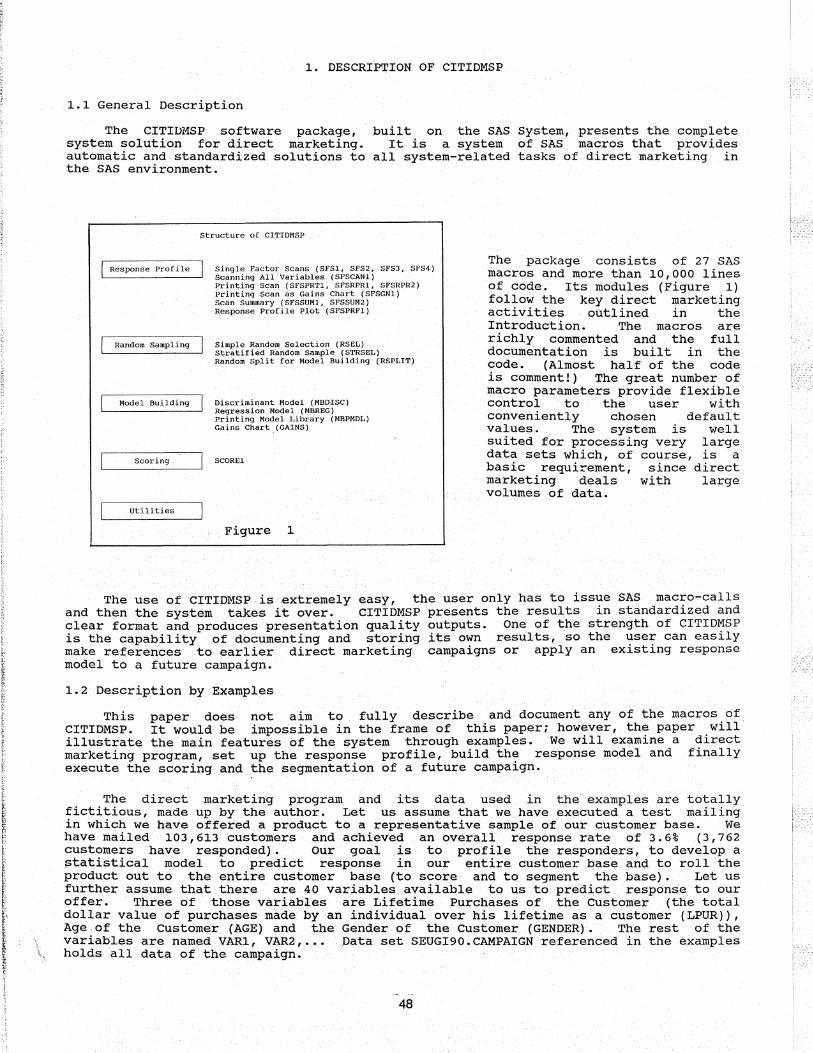
The CITIDMSP software package, built on the SAS System, presents the complete system solution for direct marketing. It is a system of SAS macros that provides automatic and standardized solutions to all system-related tasks of direct marketing in the SAS environment.
Simple Random Selection (RSEL) stratified Random Sample (ST.RSEL) . Random Split for Model Building (RSPLIT)
Discriminant Model (MBDISC) Regression Model (MBREG) Printing Model Library (MBPMDL) Gains Chart. (GA.INS)
SCOREl
Figure 1
The package consists of 27 SAS macros and more than 10,000 lines of code. Its modules (Figure 1) follow the key direct marketing activities outlined in the Introduction. The macros are richly commented and the full documentation is built in the code. (Almost half of the code is comment!) The great number of macro parameters provide flexible control to the user with conveniently chosen default values. The system is well suited for processing very large data sets which, of course, is a basic requirement, since direct marketing deals with large volumes of data.
The use ofCITIDMSPis .extremely easy, the user only has to issue SAS macro-calls and then the system takes it over. CITIDMSP presents the results in standardized and clear format and produces presehtation quality outputs. One of the strength of CITIDMSP is the capability of documenting and storing its own results, so the user can easily make referehces to earlier direct marketing campaigns or apply an existing response model to a future campaign.
1.2· Description by Examples
This paper dOeS not aim to fully describe and document any of the macros of CITIDMSP. It would be impossible in the frame of thispaperi however, the paper will illustrate the main features of the system through examples. We will eXamine a direct marketing program, set up the response profile, build the response model and finally execute the scc;>ring and the segmentation of a future campaign.
The direct marketing program and its data used in the examples are totally fictitious, made up by the author. Let us assume that we have executed a test mailing in which we have offered a product to a representative sample of our customer base. We have mailed 103,613 customers and achieved an overall response rate of 3.6% .(3,762 customers have responded). Our goal is to profile the responders, to develop a ;;tatistical model to predict response in our entire customer base and to roll the product out to the entire customer base (to score· and to segment· the base). Let us further assume .that there are 40 variables available to us to predict respOnse to our offer. Three of those variables are Lifetime Purchases of the Customer (thetotal dollar value of purchases made by an individual. over his lifetime as a customer (LPUR}), Age of the Customer (AGE) and the Gender of the Customer (GENDER). The rest of the variables are named VAR1, VAR2,... Data s.et SEUGI90. CAMPAIGN referenced in the examples holds all data of the camp~ign.
48
2. SETTING UP THE RESPONSE PROFILE.
The first questions a direct marketer raises are "Who are my responders?", "what do they look like?". In order to answer the questions, we determine the common characteristics of the responders, we set up the response profile.
2.1 The technique of Single Factor Scan
The technique of single factor scan examines a predictor variable in conjunction with response rate. It analyzes how the variable effects the binary response variable. When we set up the response profile, we execute the scan on all predictor variables and by summarizing their results, we can draw the profile of the responders relative to all customers included in the campaign.
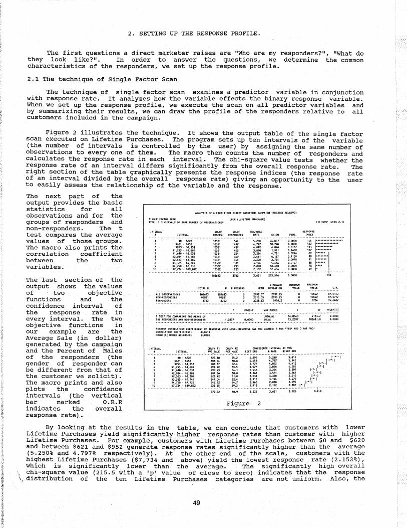
Figure 2 illustrates the teChnique. It shows the output table of the single factor scan executed on Lifetime Purchases. The program sets up ten intervals of the variable (the number of intervals is controlled by the user) by ass~gning the same number of observations to everyone of them. The macro then counts the number of responders and calculates the response rate in each interval. The chi-square value tests whether the response rate of an interval differs significantly from the overall response rate. The right section of the table graphically presents the response indices (the response rate of an interval divided by the overall response rate) giving an opportunity to the user to easily assess the relationship of the variable and the response.
The next part of the output provides the basic statistics for all observations and for the groups of responders and non-responders. The t test compares the average values of those groups. The macro also prints the correlation coefficient between the two variables.
The last section of the output shows the values of . two objective functions and the confidence interval of the response rate in every interval. The two Objective functions in our example are the Average Sale (in dollar) generated by the campaign and the Percent of Males of the responders (the gender of responder can be different from that of the customer we solicit). The macro prints and also plots the confidence intervals (the vertical bar marked O.R.R indicates the overall response rate).
ANALYSIS OF A fiCTITIOUS DIRECT MARKETING CAMPAIGN (PROJECT -SEUGI90)
SiNGLE fACTOR; SCAN lPUR (liFETIHE PURCHASE) TYPE 15 "INTERVALS Of SAME NUMBER OF OBSERVATIONS". CITIOHSP (VERS 2.1>
STANDARD MINIMUM HAXIMUH rOTAL N N N MISSING MEAN DEVIATION VALUE VALUE C.V. ....... _ ........ _ .............. _ ................... _ ....... -... -..... __ ........... -.... _ .................. _ ..... .
ALL OBSER'I!:ATIONS NOH· RESPONDERS RESPONDERS
103613 99851
3762
103613 99851 3762
2492.57 2191.25 2510.05 2198.25 2028.63 1940.2
1989'2 ,19892 m4
87.9112 87.5777 95.6407
f PROO>f VARIANCES Of PROB> I T j ....... -.. _ ...................... _ ................... -.................... _ .. -_ ......... _- .............. -._---.-. T TEST FOR COMPARING THE MEANS Of THE RESPONDERS AND NOH' RESPONDERS 1.2837 0._0000
UNEQUAL EQUAL
4133.2 1036U.0
PEARSON CORRELATION COEFFICIENT OF RESPONSE win. LPUR.-RESPONSE HAS TWO VALUES; 1 fOR 'YES' AND 0 FOR 'NO' CORRELATION COEfFICIENT: '0.0411 PROO>jR j UNDER HO:RHO=O: 0.0000
INTERVAL 08JfN #1 OUJfN #2 CONFIDENCE INTERVAL AT 90% II INTERVAL AVE_SALE PCT_HALE LEFT END R.RATE RIGHT END
By looking at the results in the table, we can conclude that customers with lower Lifetime Purchases yield significantly higher response rates than customer with higher Lifetime Purchases. For .examp·le, customers with Lifetime Purchases between $0 and $620 and between $621 and $952 generate response rates significantly higher than the average (5.250% and 4.797% respectively). At the other end of the scale, customers with the highest Lifetime Purchases ($7,734 and above) yield the lowest response rate (2.152%), which is significantly lower than the average. The significantly high overall chi-square value (215.5 with a 'p' value of close to zero) indicates that the response distribution of the ten Lifetime Purchases categories are not uniform. Also, the
49
., ~ ,
average Lifetime Purchases values of responders ($2028) and non~responders($2510) are statistically different (see the result of the t test). All these results imply that Lifetime Purchases might be a powerful predictor for response.
The values of the first objective function supply another important information: the high response rates coincide with high average sales.
2.2 Executing the Single Factor Scan
The single factor scan presented in Figure 2 is produced by the following simple macro-call:
In the macro-call, the response variable is given by parameter RESPONSE, the "yes" response is coded as 1 (parameterYESRESP), the confidence interval is calculated at 90% level (LEVEL), the name of the project is SEUGI90 (TITLE), the name of the Scan Library (see 2.5) is LIBRARY.SCAN (OUT), the intervals are printed with format DOLLARIO. and parameter OBJFUN specifies the two objective functions (AVE SALE and PCT MALE whose average values are calculated based on the responders {YMEAN}):
2.3 Types of single Factor Scans
CITIDMSP offers four types of single factor scan macros. The macros provides different ways to establish the intervals in the scans. In macro SFS1, every different
Mac::ro Technique to
SF~n Discrete SFS2 Same Number SFS3 Intervals of SFS4 User De!ined
Establish Int.ervals
of Observations Same Length Interval
value makes up one interval. Macro SFS2 establishes the intervals (their number is specified by the user) such that every interval has the same number of obserVations. Macro SFS3 sets up intervals with the same lengths. Finally, in macro SFS4, the intervals are specified by the user with the
help ofa user defined SAS format. A numeric variable can be scanned with any of the four macros, but a character variable can be scanned only with macros SFSI and SFS4.
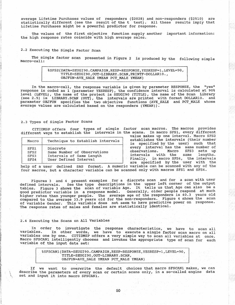
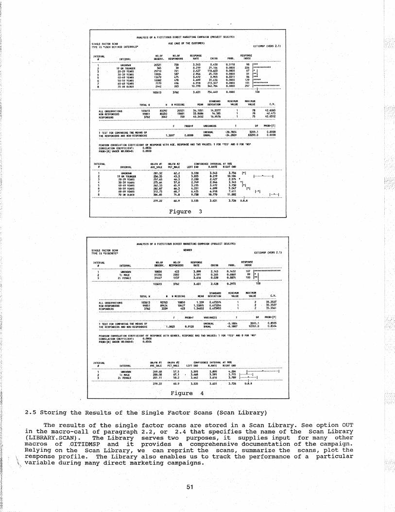
Figures 3 and 4 present exampJ,es . for a discrete scan and for a scan with user defined intervals. See the type descriptions in the upper left corner of the output tables. Figure 3 shows the scan of variable Age. It tells us that Age can also be a good predictor variable in a response model. Generally, older peopl~ respond at much higher rates than younger p·eople. The average age of the respon~ers l.S 40.3 years old compared to the average 33.9 years old for the non-responders., F:gure 4 shows the scan of variable Gender. This variable does not seem to have predl.ctl.ve power on response. The response rates of males and females are statistically identical.
2.4 Executing the Scans on All variables
In ord~rto investigate ~he response characteristics, we have t scan all variables. . In other words, we have to execute a single factor scan m~~ro on all variables one by one. CITIDMSP offers a very simple way to scan all variables at once. Macro SFSCANl intelligently chooses and invokes the appropriate type of scan for each variable of the input data set:
If we want to overwrite the default choices that macro SFSCAN1Iilakes, we can \ describe the paramet.ers of every scan or certain scans only, in a so-called engine data \. set and input it into macro SFSCAN1. "
50
AJlAlYSIS Of A fiCTITIOUS DIRECT WUTlNG CAMPAIGN (PROJ~CT SEUGI90)
AGE (AGE Of THE CUSTotER) SINGle fACTOR SCAN TYPE IS "USER DEfiNED INTERVALS" cIT IDMSP (VERS Z.1)
;.;~;;.;~.~;;;;;.;~.~;.;;~;,; .............................. ·········;,;~········:20:m;.·········i209:,······0:0000 T"E RESPONOEIS AND NOU·RESPONDERS 1.3897 0.01100 EQUAL. '24.2029 83290.0 0.00011 ............................................................................................................................. PEARSON CORRELATION COEffiCIENT OF RESPCWSE WITH AGE. RESPONse HAS TWO VALUES-: 1 FDA 'YES' AND 0 FOA 'MOt CORRELATION COEFFICIENT: O.Dal6 PRCJJ)oIRI UNDER HO:I"OIIO: 0.0000
INTERVAL OOJFN " OBJfN 112 CONFIDENCE INTERVAL AT 901
2.5 storing the Results of the Single Factor Scans (Scan Library)
The results of the single factor scans are stored in a scan Library. See option OUT in the macro-call of paragraph 2.2, or 2.4 that specifies the name of the Scan Library (LIBRARY.SCAN). The Library serves two purposes, it supplies input for many other macros of ,OITIDMSP and it provides a comprehensive documentation of the campaign. Relying on the Scan Library, we .can reprint the scans, summarize the scans, plot the
" response profile. The Library also enables us to track the performance of a particular \. variable during many direct marketing campaigns. ,.
51
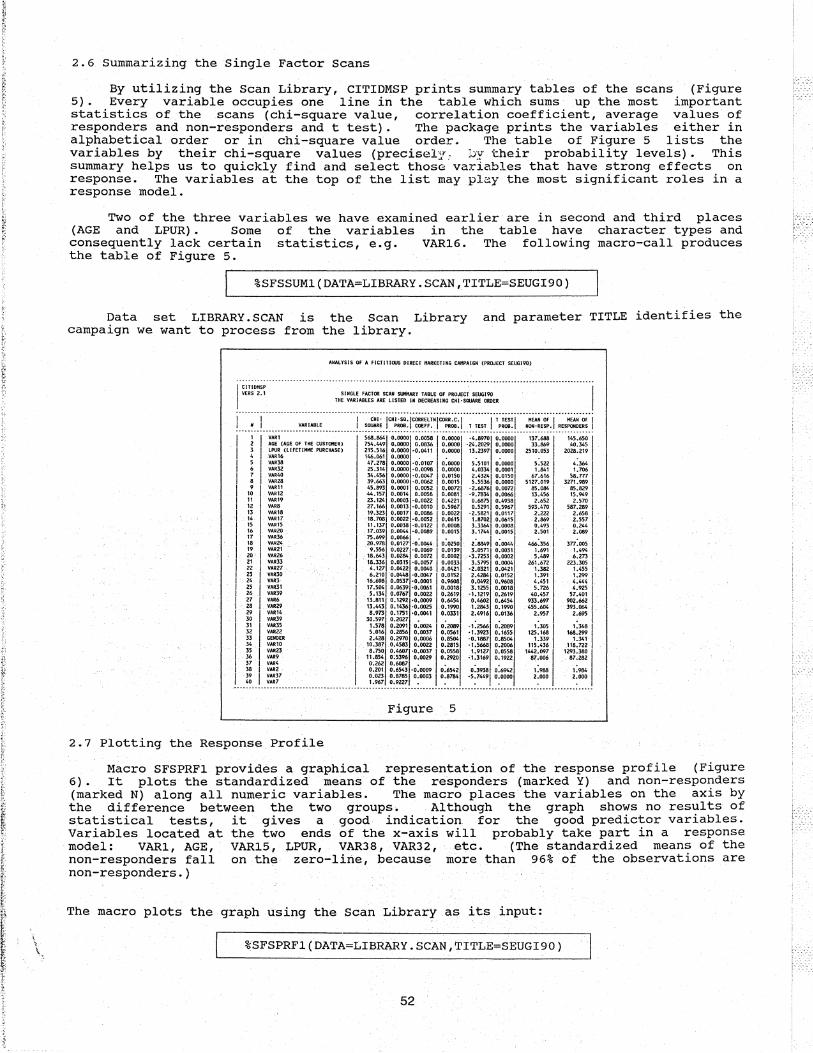
2.6 summarizing the Single Factor Scans
By utilizing the Scan Library, CITIDMSP prints summary tables of the scans (Figure 5). Every variable occupies one line in the table which sums up the most important statistics of the scans (Chi-square value, correlation coefficient, average values of responders and non-responders and t test). The package prints the variables either in alphabetical order or in chi-square value order. The table of Figure 5 lists the variables by their chi-square values (precisel::,', l.)y their probability levels). This summary helps us to quickly find and select those variables that have strong effects on response. The variables at the top of the list may play the most significant roles in a response model.
Two of the three variables we have examined earlier are in second and third places (AGE and LPUR). Some of the variables in the table have character types and consequently lack certain statistics, e.g. VAR16. The following macro-call produces the table of Figure 5.
%SFSSUMl (DATA=LIBRARY. SCAN,TITLE=SEUGI90)
Data set LIBRARY.SCAN is the Scan Library and parameter TITLE identifies the campaign we want to process from the library.
ANALYSIS Of A FICTITIOUS DIRECT MARKETING CAHPAIGH'(PROJECT SEUGI90)
Figure 5
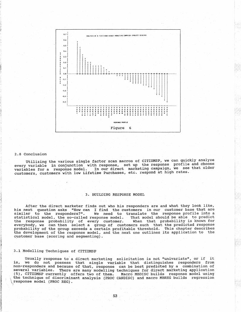
2.7 Plotting the Response Profile
Macro SFSPRFl provides a graphical representation of the response profile (Figure 6). It plots the standardized means of the responders (marked Y) and non-responders (marked N) along all numeric variables. The macro places the variables on the axis by the difference between the two groups. Although the graph shows no results of statistical tests, it gives a good indication for the good predictor variables. Variables located at the two ends of the x-axis will probably take part in a response
. model: VAR1, AGE, VAR15, LPUR, VAR38, VAR32, etc. (The standardized means of the non-responders fallon the zero-line, because more than 96% of the observations are non-responders.)
The macro plots the graph using the Scan Library as its input:
%SFSPRF1(DATA=LIBRARY.SCAN,iI'ITLE=SEUGI90)
52
2.8 Conclusion
I Q.7 +
I ANALYSIS OF A FlC1"JtlOUS OIRECT MRKEiING CAMPAIGN (PROJECT SEUGIW)
0.6 +
I ' 0.5· I
I II 0.4 + II I , 0.3 i I I II 0.2 i 1111 r j yy yy
0.1 i I " " I 11111 ; , .::~ r················································,··,··:··:··:·TTIIlllTr·il·lll···ll··II ...... · .. · '0.2 i ' , , ) I I II '0.3 ~ 'I I I ,0.4! ) ) , 1\
V A V Y V V " Y Y 'y V V G Y Y V V Y Y Y V V .V V V V Y V V V V V V l V A G A A A A A A A A A A E A A A A A A A A A A A A A A A A A A A A p'" RERRRRRRRRRRIfRRftRRRRRRRRRRRRRRRRRUR 1 1 2 1 1 2 2· 9 1 3 3 D 3 3 2 6 8 1 2 2 1 2 3 4 1 1 1 2 2 2 3 3 R 1
utilizing the various single factor scan macros of CITIDMSP, we can q';1ickly analyze every variable in conjunction with response, set up the response prof1le and choose variables for a response model. In our direct marketing campaig~, we see that older customers, customers with low Lifetime Purchases, etc. respond at h1gh rates.
3. BUILDING RESPONSE MODEL
After the direct marketer finds out who his responders are and what they look like, his next question asks "How can I find the customers in our customer base that are similar to the responders?". We need to translate the response profile into a statistical model, the so-called respons~ model. That model should be able to predict the response probability of every customer. When that probability is known for everybody, we can then select a group of customers such that the predicted response probability of the group exceeds a certain profitable threshold. This chapter describes the development of the response model, and the next one outlines its application to the customer base (scoring and segmenting). . .
3.1 Modelling Techniques of CITIDMSP
Usually response to'a direct marketing solicitation is not "univariate", or if it is, we do not possess that single variable ·that distinguishes responders from non-responders and because of that, response can be best predicted by a combination of several variables. There are many modelling techniques for direct marketing application {5}, CITIDMSP currently offers two of them. Macro MBDISC builds response model using
\ the technique of discriminant analysis (PROC CANDISC) and macro MBREG builds regression \,response model (PROC REG) • ,
53
3.2 selecting variables for the Response Model
As the first step of the model building, we have to select the variables for inclusion. There are many considerations, the penetration of the variable in the customer base, its historical performance, its reliability (internal vs. external), etc. The results of the single factor scans give us the potential model variables: variables with the highest chi-square values, or variables with the highest correlation coefficients. Since the single factor scan is a univariate technique only, we also need the help of certain mUltivariate methods, to select the best variables based on their simultaneous effects on response. For example, we can utilize PROC STEPDISC or PROC STEPWISE to choose our model variables.
3.3 Building the Model
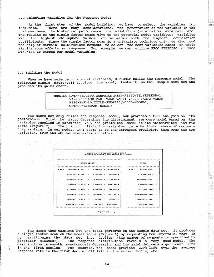
When we have selected the model variables, CITIDMSP builds the response model. The following single macro-call develops the model, tests it on the sample data set and produces its gains chart.
The macro not only builds the response model, but provides a full analysis on its performance. First the macro determines the discriminant response model based on the variables supplied in parameter VAR, and prints the model in its standardized and raw forms (Figure 7). The printout lists the variables in order their share of variance they explain. In our model, VARI seems to be the strongest predictor, then come the two variables, LPUR and AGE we have examined before.
I
ANALYSIS OF A fiCTITIOUS DIRECT MARKETING ~PAIGN STANDARDIZED AIlD RAY FORMS Of MOOEL MaJE'L1 OF PROJECT SEUGI90
ST AHDARD I ZED fORM RAW' FORM I .................................................................................. . ........................................ . I SCORE" D.695080sn * ( VAK1 1.766224616) I 0.4232330124 ... I
II :::: ::: '~:::: :=: I
'0.369368166 ... ( VARl8 1.364074203 J I D.48117191S5 ...
0.3563684497 ... ( VAR28 3.977559648 ) I 3.492561649 +
I I
I 1.994151031 ) I 0.07625493344
I D.0001S893J ... LPUR ... I
·0.01107912902 .. AGE
-0.767642819 ... VAR38 + I 0.1020364092 ... VAR28 +
O.OOOl1610786n • VAH" • I 0.02951962515 .. VAR;t ... I
1.04312.7882 .. VAR8
0.2769465231 ." ( V~R32 , 1387.864615, ) I 876.1139847 +
SCORE = 1.642311804 ." VAR1
0.2692859821 "'« VAR11 17.5011"7752) I 9.122269701 +
0.07954364718 ." ( VAR8
Figure 7
The macro then examines how th~model performs on.~he sample data s~t~ It p:r;oduces a single factor scan on the model score ·(Figure 8) by requesting ten iritervals, that is by partitioning the data set into· deciles . (the number ofsegritents is specified by param~ter NSEGMENT). The responsedistributiori. reveals a very good model .. The distribution is smooth, monotonollslydecreasing and the model delivers significant lifts in the first·deciles. For example, the model provides 229% lift over the average response rate in the first decile, 62% lift in the second decile, etc.
54
ANALYSIS OF A FICTITIOUS DIRECT MARKETING CAMPAIGN (PROJECT SEUGI90)
SINGLE FACTOR SCAN SCORE (SCORE OF THE RESPONSE MOOEL) TYPE IS I+INTERVAlS Of SAME NUMBER OF OBSERVATIONS"
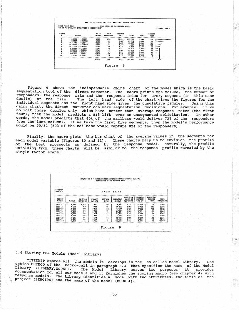
Figure 9 shows the indispensable gains chart of the model which is the basic segmentation tool of the direct marketer. The macro prints the volume, the number of responders, the response rate and the response index for every segment (in this case decile) of the file. The left hand side of the chart gives the figures for the individual segments and the right hand side gives the cumUlative figures. Using this gains chart, the direct marketer can make segmentation decisions. For example, if we solicit those deciles only which have better than average response rates (the first four), then the model predicts a 81% lift over an unsegmented solicitation. In other words, the model predicts that 40% of the mailbase would deliver 73% of the responders (see the last column). If we take the first five segments, then the model's performance would be 50/82 (50% of the mailbase would capture 82% of the responders).
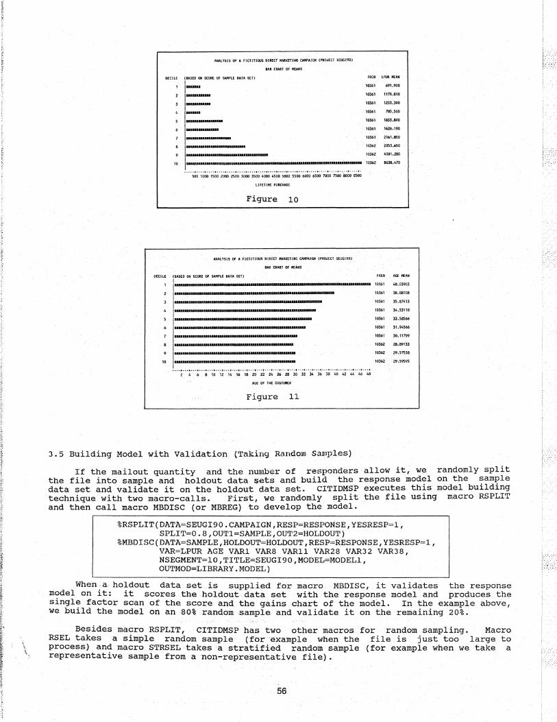
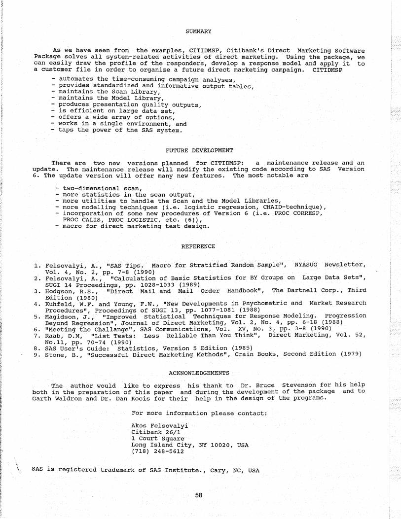
Finally, the macro plots the bar chart of the average values in the segments for each model variable (Figures 10 and 11). These charts help us to envision the profile of the best prospects as defined by the response model. Naturally, the profile unfolding from these charts will be similar to the .response profile revealed by the single factor scans~
ANALYSIS OF A FICTITIOUS DIRECT MARKETING CAMPAIGN (PROJECT SEUGI90) PERFORMANCE OF THE RESPONSE MOOEl
I CtTltiHSP VERS2.1 GAINS' CKART
................................................. -~ .... _. _ .. _. -......... _ ......... _ .... -............ _ ...... '-" .... _ ..... --., ...... . 1 SEGMENT I I NUMBER OF I RESPONSE I RESPONSE I CUMULATIve I c:!:~T~ I ~~~~~E I C::~~~E I MOOEl I ! ... ~~~~~. _.! ... ~~ ~~~ .. !. ~~~~?~~~.! .. ~~~~. ~~~ .. !. _ .. ~~~~ ... ! -.. ~~ ~~~ _.!. ~~~~~~~~~.! .. ~~:~. ~~~ ....... ~~~~ ... !~~~~~~~::!
DECILE 1
I 10,361 I 1,238 11.949 329 I ~:~~ I 1.238 I 11.949 329 10/33
DECILE 4 10,361 402 3.880 107 2,730 6.587 181 40/73 DECILE 5 I 10,361 I '60 3.475 96 !~:~c11 3,090
I 5.965 164 50/82
OECTI:E 6 10.361 198 1.911 '3 3,Z88 5.289 146 60/87 DECilE 7 I ~~:~:; I I.' 1.682 52
I ~~:!!~ I 3,483 4.802 '" 70/93 DECilE 8 16.1 1.554 " 3,M4 4.396 121 80/97 OECllE 9 I 10,362 I 100 0.965 27 l~~:~~i I 3,744 I 4.015 111 90/10() DECILE 10 10,362 18 0.174 , 3,762 3.631 100 _lOa/IDa ................................................ -...... .....................................................................
Figure 9
3.4 storing the Models (Model Library)
CITIDMSP stores all the models it develops in the so-called Model Library. See option OUTMOD of the macro-call in paragraph 3.3 that specifies the name of the Model Library (LIBRARY.MODEL). The Model Library serves two purposes, it provides documentation for all our models and it furnishes the scoring macro (see chapter 4) with res~onse mOdels. The Library identifies a model with two attributes, the title of the proJect (SEUGI90) and the name of .the model (MODELl).
55
f f r ': ~:
1 " r ~" ~:
l. ,. ~ ~
~ ~ [ ~~
1; f ~ ~ ~.
" ~;
~
* ~. ~
~
i :i
f,
I \ ~.
\. "
~
~ ~ :t .:~
ANALYSIS OF A FICTITIOOS DIRECT MARKETING CAMPAIGN (PROJECT SEUGI-90)
BAR CHART Of HEARS
DECilE (BASED ON SCCltE OF SAMPLE DATA SET) I '1_ 21_
31==-· 61 __ _
7 I .......... • ........ I 81====--10 1_~.,U __ .... _ ... _ ........ H __ ... _ ..... ua_ ...... II ......
3.5 Building Model with Va l£clCl,tiOl1. ('faking RandOltl SaropJ,es)
48.03903
38.88108
35.87413
34.53110
33.58566
31.94566
30.11199
28.89133
Z9.57538
Z9.59595
If the mailout quantity and'the riumber of responders allow it; we randomly split the file into sample and holdout data sets and build the response model on the sample data s.et and validate it on the holdout data set. CITIDMSP executes this model building teChnique with two macro-calls. First, we randomly split the file using macro RSPLIT and then call macro MBDISC (or MBREG) to develop the model.
%MBDISC(DATA=SAMPLE,HOLDOUT=HOLDOUT,RESP=RESPONSE,YESRESP=l, VAR=LPUR AGE VARI VAR8 VARll VAR28 VAR32 VAR38, NSEGMENT=10,TITLE=SEUGI90,MODEL=MODELl, OUTMOD=LIBRARY.MODEL)
Whena. holdout data set is supplied for macro MBDISC, it validates the response m<?delon it: it scores theholdout.data set with the response model and produces the sl.ngle factor scan of the score and .. the gains chart of the model. In the example above, we build the model on an80%random.sample and validate it on the remaining 20%.
Besides macro RSPLIT, CITIDMSPhas two other macros for random sampling. Macro RSEL takes a simple random sample (fOrexample when the file is just too large to process) and macro STRSEL takes a stratified random sample (for example when we take a representative sample from anon-representative file).
56
3.6 Conclusion
With the help of the model building macros of CITIDMSP, we can easily develop a response model, validate it and compile its gains chart for further segmentation. In our example, we have fabricated a powerful response model that predicts SUbstantial lifts in the best deciles. It is a 50/82 model, that is by mailing the upper half of the ~u~tomer base we can captures 82~ of all potential responders. (The problem of d7cl1n1~g response rate of the rollout 1S beyond the scope of this paper. See {7} for a d1scuss10n. )
4. SCORING, SEGMENTING
When the direct marketer clearly pictures his responders and possesses a powerful response model, he wants to apply the model to his customer base and to "rollout" the product. CITIDMSP effortlessly scores and segments the customer file.
4.1 scoring and Segmenting the Customer Base
The following macro-call scores the customer Base and partitions the file into segments of different response rates.
The parameters identify one model of the Model Library to be used (parameters TITLE and MODEL), specify the number of segments we want to create (NSEGMENT) and the names of the variables that hold the segment numbers (SEGMENT) and the score,values (SCORE). In our example, we take the model from the Model Library we developed 1n Chapter 4 (called MODELl) and apply it to the . customer Base. After . scoring all customer~, the ma~ro assigns them to ten segments, to thedeciles.Adcord1ngtothemodel,·thef1rst dec1le has the highest probability of response (it is 3.29 times higher then the response rate of the entire file) then COmes the second decile and So on.
4.2 creating the Mailing File
Macro STRSEL (macro for stratified random sample) can create us the mailing file of our rollout. Based on the model's gains chart (Figure 9), we decide which segments we want to include in the rollout and the macro selects them for us. Let us select the first five deciles entirely and also let use take a 5% random sample from every decile from 6 to 10 for model validation purpose. The following statements create the mailing file.
\ ' The program creates a mailing file with three ~ariables (ID, NAME, and ADDRESS) by \ tak1ng all c~stomer~ from the first fivedeciles and 5% of the customers randomly from -"the second f1ve dec1les. --
57
~ ." ~~ ~-' i
~ ~
SUMMARY
As we have seen from the examples,CITIDMSP, citibank's Direct Marketing Software Package solves all system-related activities of direct marketing. Using the package, we can easily draw the profile of the responders, develop a response model and apply it to a customer file in order to organize a future direct marketing campaign. CITIDMSP
- automates the time-consuming campaign analyses, - provides standardized and informative output tables, - maintains the Scan Library, - maintains the Model Library, - I?roduc7s,Presentation quality outputs, - ~s eff~c~ent on large data set, - offers a wide array of options, - works in a single environment, and - taps the power of the SAS system.
FUTURE DEVELOPMENT
There are two new versions planned for CITIDMSP: a maintenance release and an update. The maintenance release will modify the existing code according to SAS Version 6. The update version will offer many new features. The most notable are
1.
2 · 3 · 4 · 5 · 6 · 7 · 8 9 ·
- two-dimensional scan, - more statistics in the scan output, - more utilities to handle the Scan and the Model Libraries, - more modelling techniques (i.e. logistic regression, CHAID-technique), - incorporation of some new procedures of Version 6 (i.e. PROC CORRESP,
PROC CALIS, PROC LOGISTIC, etc. (6}), - macro for direct marketing test design.
REFERENCE
Felsovalyi, A., "SAS Tips, Macro. :for stratified Random Sample", NYASUG Newsletter, Vol. 4, No.2, pp. 7-8 (1990) Felsovalyi, A., "Calculation of Basic. statistics for BY Groups on Large Data sets", SUGI 14 Proceedings, pp. 1028-1033 (1989) Hodgson,R.S., "Direct Mail and Mail Order Handbook", The Dartnell Corp., Third Edition (1980) Kuhfeld, W.F. and Young, F.W., "New Developments in psychometric and Market Research Procedures", Proceedings of BUGI 13, pp. 1077-1081 (1988) Magidson, J., "Improved statistical Techniques for Response Modeling. progression Beyond Regression", Journal of Direct Marketing, Vol. 2, No.4, pp. 6-18 (1988) "Meeting the Challange", SAS Communications, Vol. XV, No.3, pp. 3-8 (1990) Raab, D.M, "List Tests: Less Reliable Than You Think", Direct Marketing, Vol. 52, No.ll, pp. 70-74 (1990) SAS User's Guide: Statistics, Version 5 Edition (1985) Stone, B., "Successful Direct Marketing Methods", Crain Books, Second Edition (1979)
ACKNOWLEDGEMENTS
The author would like to express his thank to Dr. Bruce Stevenson for his help both in the preparation of this paper and during the development of the package and to Garth Waldron and Dr. Dan Kocis for their help in the design of the programs.
For more information please contact:
Akos Felsovalyi Citibank 26/1 1 Court Square Long Island City, NY 10020, USA (718) 248-5612
SAS is registered trademark of SAS Institute., Cary, NC, USA