City-Location and Sell-Side Analyst Research

by

Joshua L. Gunn

University of Pittsburgh

Draft Date: August 2014

City-Location and Sell-Side Analyst Research

ABSTRACT: I find that analysts’ earnings forecasts are more accurate and the stock market

reaction to analyst reports is stronger when the analyst is located in a city with higher human

capital. Human capital is proxied for as the average education-level in the city. These results are

consistent with prior theoretical and empirical research in the urban economics literature that links

a higher average education of a city’s work force with externalities and knowledge spillovers that

increase productivity. These findings contribute to the literature investigating the effect of

geography on information flows and analyst performance by expanding the discussion to the

attributes of particular geographic locations.

Keywords: Human capital; analyst informativeness; forecast accuracy

Data Availability: Data used are publicly available from sources identified in the paper.

Acknowledgments

I am grateful to my dissertation committee, Jere Francis (co-chair), Inder Khurana (co-chair),

Raynolde Pereira, and John Howe, as well as workshop participants at the University of Missouri,

for many helpful comments and suggestions that have improved this paper.

1

City-Location and Sell-Side Analyst Research

1. Introduction

Equity analysts are important information intermediaries in the capital markets that engage

in private information acquisition and provide analysis to investors, and their reports are

potentially important to improving the informational efficiency of capital markets (Frankel et al.,

2006). To issue these reports, analysts must acquire, process, and summarize a significant amount

of knowledge. Prior research has found that the informativeness and accuracy of analyst reports

vary predictably with different analyst attributes and characteristics of their information

environment, such as reputation (Stickel, 1992), ability (Sinha et al., 1997), experience (Clement,

1999; Clement et al. 2007; Mikhail et al., 1997), brokerage firm size (Clement, 1999; Jacob et al.,

1999), number of firms followed (Clement, 1999; Hirst et al., 2004), and industry expertise (Jacob

et al., 1999).

In addition, researchers have found that geography plays an important role in the flow of

information. For example, Coval and Moskowitz (1999) find that information asymmetry drives a

preference for geographically proximate investments by U.S. mutual fund managers, and Malloy

(2005) documents that analyst forecasts are more accurate and informative when there is less

distance between the analyst and the firm. I extend this line of inquiry by investigating the

association between analyst performance and the average education of the city in which the analyst

works. Prior research on economic geography in the accounting and finance literatures largely

focuses on distance (e.g. the distance between the analyst/investment manager and a particular

firm), but location also marks differences in other factors potentially relevant to the analyst’s

information environment.

Research in urban economics finds that the human capital depth in a geographic area,

proxied as the average education level, speeds the flow of ideas and creates knowledge spillovers

that result in positive economic outcomes (Moretti, 2004b). Because they are dependent on

2

acquiring and processing information to produce their reports, analysts are a good example of the

type of knowledge workers who should benefit from human capital externalities. Jacobs (1969)

argues that a key role of learning in cities is due to their ability to bring in a set of diverse firms

because the most important source of knowledge spillovers is external to the industry, not within

the industry. Lucas (1988) notes that the advantages of cities for learning are not only related to

cutting-edge technologies, but also the acquisition of everyday skills and knowledge accumulation.

In this sense, human capital externalities could make analysts more productive by providing more

precise information or by making them more efficient processors of information through the

acquisition of such skills. I hypothesize that these human capital externalities create a source of

variation in the information available to individual analysts, which in turn, affects their

productivity.

To test whether human capital externalities make analysts more productive, I investigate

the association between the informativeness and accuracy of analyst reports and the average

education of the city in which the analyst is located. I predict that analysts located in cities with

higher human capital will issue reports that are more accurate (smaller absolute value forecast

errors) and more informative (larger stock market reaction to recommendation changes and

forecast revisions). The results of my empirical analysis are consistent with these predictions.

Using a panel data set of individual analyst forecasts and recommendations from 2002 to 2008, I

find robust evidence that the accuracy and informativeness of analyst reports are increasing in city-

level human capital.1 More specifically, I find that the absolute value of relative forecast errors

decreases by 2.27% with a one standard deviation change in average human capital. In addition,

abnormal trading volume on the day an analyst report is issued increases by 5.66% to 15.62% with

1 I obtain information on individual analyst’s location from Nelson’s Directory of Investment Research, but this

directory is no longer published after 2008.Therefore, data availability limits my sample to 2008 and earlier. See

Section 3 for more detail on sample construction.

3

a one standard deviation change in the percent of people with a college degree in the analyst’s city,

depending on the type of analyst report issued (i.e., recommendation change or forecast revision)

and whether the report conveyed good or bad news. Finally, industry-size adjusted stock returns

on the day an analyst report is issued are larger by 0.07% to 0.27% (in absolute magnitude) with a

one standard deviation change in average human capital. Because almost half of all sell-side

analysts are located in New York, I report all analyses both with and without these analysts, and

the results are virtually the same.2 In addition, the results are robust to controlling for a variety of

analyst-related characteristics that prior literature has shown to be associated with analyst

performance as well as city-level factors that might be associated with productivity differences.

This paper contributes to the research literature in several ways. First, a significant body of

literature is devoted to understanding analysts and their role in the capital markets (Bradshaw,

2011). As noted above, this has led researchers to document several attributes of analysts and their

information environments which affect their ability to provide informative and accurate research.

At the same time, accounting and finance studies have begun to explore the role that economic

geography plays in the capital markets (Coval and Moskowitz, 1999; Malloy, 2005). One

contribution of this paper is to document an additional source of variation in analyst performance

that links their information environment to their location in geographic space. In doing so, I attempt

to shed some light into the “blackbox” of how analysts gather and process information (i.e.,

through interactions with other people), which Bradshaw (2011) argues is necessary to move the

literature forward. Nonetheless, that blackbox is still very dark, and there are several questions

beyond the scope of this study that remain unanswered. For example, while I make some

conjectures as to the mechanisms through which average city-level human capital is translated into

more informative and accurate analyst reports, my archival research setting limits my ability to

2 In untabulated analyses, I find that the results are also robust to deleting analysts located in San Francisco and

Chicago, the cities with the second and third highest number of analysts.

4

directly test these potential mechanisms. As such, the evidence presented in this paper should be

interpreted as suggestive of the hypothesized relationships, rather than definitive evidence of

causality, similar to other studies employing such cross-sectional research designs (Bushman et

al., 2004). Section 5 discusses this issue in more detail. Future research may be able to explore

these issues further, perhaps using different research designs.

This paper also contributes to the research literature investigating the economic

consequences of human capital externalities by documenting an additional real economic outcome

of local knowledge spillovers – the incorporation of local information into security prices. Moretti

(2004b) notes that while there is theoretical and empirical support for the existence of human

capital externalities, economists have not yet reached a consensus on their economic magnitudes.

I extend research on human capital externalities to equity analysts, and suggest an additional way

through which human capital externalities can affect economic activity.

Finally, the results of this paper should also be of interest to practitioners. Similar to many

other service industries, outsourcing in financial services has become increasingly common, to the

extent that even more complex tasks, such as junior-level analyst work, are now seen as potential

candidates for outsourcing (Benson, 2010). What tasks can and should be outsourced, and where

they should be outsourced to, will continue to be important questions for the industry as this trend

continues, especially as educational levels rise in parts of the developing world. While the results

of this study do not provide definitive answers to these questions, they do point to several cost and

benefits to location choice that could be potentially relevant for the industry.

The rest of this paper proceeds as follows. Section 2 provides more background on the

analyst and human capital research literatures, and formally states my hypotheses. Section 3

describes the empirical models, sample selection, and data. Section 4 presents the results of the

empirical analysis. Section 5 discusses some robustness tests and caveats. Section 6 concludes.

5

2. Background and Hypothesis Development

2.1 Background on Analyst Research

Several prior studies argue that analysts provide useful information to the markets (e.g.,

Womack, 1996; Barber et al., 2001; Jegadeesh et al., 2004). Researchers have also documented

that analysts’ ability to provide useful information to the markets varies predictably with their

ability to gather and/or process information.3 For example, several papers have hypothesized that

analyst performance is associated with experience. Clement (1999) and Mikhail et al. (1997) find

that forecast accuracy is positively related to analysts’ firm-specific forecasting experience

(proxied as the number of years the analyst has been following a specific firm). Comparing the

effects of firm-specific and general experience, Clement (1999) concludes that firm-specific

experience is more important, although Jacob et al. (1999) find that the effect of experience goes

away after controlling for analysts’ innate ability in a fixed effects regression.

Clement et al. (2007) find that the most relevant type of experience is task-related, not firm-

or industry-related. They suggest that analysts learn by performing specific tasks, such as

forecasting earnings for firms undergoing restructurings, and this task-specific experience is more

relevant to analyst performance than industry- or firm-related experience. Clement et al. (2007)

and Jacob et al. (1999) both report that analysts who specialize in specific industries (measured as

the concentration of firms followed in a particular industry) perform better. Clement (1999) and

Hirst et al. (2004) find that analyst performance decreases when they follow more firms,

suggesting that analysts reduce their average firm-specific knowledge if they follow too many

3 There are other factors which influence the accuracy and informativeness of analyst reports, such as company-

related-factors (e.g. size), and characteristics of the reports themselves (e.g. forecast horizon). I discuss these

variables in Section 3 when I introduce my control variables. Because the analyst literature is so large, I focus this

section specifically on attributes of analysts and their information environment, as I consider this segment of the

analyst literature to be most relevant to my study.

6

firms. Similarly, Clement et al. (2007) report some mixed evidence that analysts who follow more

industries reduce their forecast accuracy on average.

Several papers find that analysts who work for larger brokerage firms issue more accurate

and informative reports, suggesting that analysts are more productive when they work for

brokerage firms with more resources at their disposal (e.g. Clement et al., 2007; Jacob et al.,

1999).4 With regard to innate ability, Brown (2001) finds that a model using analyst past accuracy

performs as well as using analyst characteristics in identifying superior analysts, suggesting that

analyst performance is somewhat sticky over time. Stickel (1992) reports evidence that analysts

who are named to Institutional Investors All-America team issue more accurate forecasts and that

the stock market reaction to their forecast revisions is stronger than other analysts. Jacob et al.

(1997) use an analyst fixed effects model to control for innate ability and conclude that innate

ability is a more important determinant of analyst performance than experience.

Finally, Malloy (2005) integrates the study of economic geography into the analyst

literature by finding that reports issued by analysts who are geographically proximate to the firms

they are following are more accurate and informative than analysts who are further away. This

suggests that analysts can gain information advantages about specific firms when they are

physically close to them. These findings are consistent with prior research by Coval and

Moskowitz (1999), who find that U.S. investment managers have a preference for locally

headquartered firms, especially small and highly levered firms. Coval and Moskowitz (1999)

conclude that asymmetric information drives a preference for geographically proximate

investments because proximity leads to information advantages.

This study contributes to the analyst literature by linking research on attributes of the

analyst’s information environment to studies of economic geography. Geographic location can be

4 I refer to the company which the analyst is following and issuing reports about as the “company” or the “firm.”

The company that employs the analyst is always referred to as the “brokerage firm” in the text.

7

used to define the distance between two parties in the capital markets (e.g., the analyst/mutual fund

manager and the firm that they are following), but it also marks differences in average human

capital. As noted below, a separate stream of research provides theoretical and empirical evidence

that human capital externalities create positive economic outcomes through knowledge spillovers.

2.2 Background on Human Capital Externalities

Research on human capital externalities has grown out of the urban economics literature,

which can be broadly defined as trying to answer the question, “why do cities exist?” This is an

interesting question because economic activity continues to be heavily concentrated in a relatively

small geographic area, despite the considerable costs associated with living and working in cities

(e.g. crime, congestion, higher rents, etc.) and technological advances that have made

transportation and communication across large distances cheaper than ever before (Krugman,

1991; Glaeser, 2011). While workers can be compensated for the higher costs of living in cities

through increased wages and/or cultural and social amenities, it is harder to explain why firms

would choose to continue locating in cities (Moretti, 2004). Without some benefit that accrues to

the firm, cities should “fly apart” in the face of these economic forces (Lucas, 1988).

Agglomeration economies are the mechanism through which this concentration of economic

activity persists. Agglomeration economies exist when productivity increases with density. If

workers are more productive in cities, this would help firms bear the costs of locating in urban

areas. Human capital externalities can be considered a subset of the research on agglomeration

economies and explain one potential benefit arising from geographic concentration.

Agglomeration economies arise by reducing transportation costs. This includes not only

the transportation of goods, but also of ideas and knowledge between individuals. Glaeser and

Gottlieb (2009) argue that modern cities survive by speeding the flow of ideas between people.

Studies such as Glaeser (1999), Jovanovic and Rob (1989), and Lucas (1988) provide the

8

microeconomic foundation for these local knowledge spillovers. In these models, new ideas are

generated as individuals interact with each other. As the average level of human capital

(knowledge) increases, individuals have more “luck” at gaining productive knowledge from

others. An important point in these models is that knowledge spillovers depend on both the

intensity of the search for new knowledge and the vertical differences in what people know. “If all

of us know the same thing, we cannot learn from each other.”(Jovanovic and Rob, 1989, p. 569)

Building on this theoretical work, several empirical studies have tried to measure whether

the vertical difference of knowledge in a particular place, or what is termed human capital depth

(Fu, 2007), is related to productivity. Because the microeconomic models discussed above show

that the “luck” that an individual has of learning a new idea is a function of the average human

capital of the people that the individual interacts with, a common empirical proxy in this research

is the average education level of the city in which the individual works. The average education of

a city has been found to be associated with higher wages (Rauch, 1993), patent generation (Glaser

and Saiz, 2004), and service firm formation rates (Acs and Armington, 2004). Moretti (2004a)

uses longitudinal data on individual wages over a long sample period to address some of the more

serious endogeneity threats in this line of research (such as individuals potentially sorting into

cities based on unobserved ability). He continues to find an association between individual wages

and average education level and finds little support for individuals self-sorting into high human

capital cities based on unobserved ability. Overall, Moretti (2004b) surveys the literature and

concludes that there is both theoretical and empirical support for the existence of human capital

externalities, although researchers have not reached a consensus as to their economic magnitudes.

2.3 Why would equity analysts benefit from human capital externalities?

Jovanovic and Rob (1989) conclude that knowledge spillovers depend upon the vertical

integration of knowledge. In order for equity analysts to benefit from knowledge spillovers, they

9

would need to interact with others who know something that they do not already know. To get a

sense for how these knowledge spillovers might happen in practice, it is useful to gain an

understanding of what analysts do on a daily basis. Appendix A contains excerpts from four

webpages and blog posts identified using two internet searches: “a day in the life of an equity

analyst” and “what does an equity research analyst do.” The purpose of this exercise is to

understand what analysts do on a daily basis, who they interact with, and how they might benefit

from local knowledge spillovers. For interested readers, I have retained the entire text of the

internet posts in Appendix A. The excerpts that I discuss below are highlighted with bold and italic

text in the appendix.

While obviously anecdotal, there are several points in these descriptions of analysts’ duties

that highlight the importance of developing information sources from others with different

knowledge bases than the analyst. For example, Example 1 provides a job description and opinion

about what makes a sell-side analyst successful. To generate revenue, the author believes that a

sell-side analyst must be seen as providing valuable information. Since “nobody cares about the

third iteration of the same story….there is tremendous pressure to be the first to the client with

new and different information.” The author of Example 1 goes on to discuss the importance of

creating “expert networks...anybody can call a doctor or engineer, but the best sell-side analysts

know the right ones to call.” Example 2 describes a “typical” day for an analyst who appears to

follow the Biotechnology sector. A busy day includes a discussion (in this case a conference call)

with a doctor who is a lung cancer specialist to understand recent clinical trials. Example 3 presents

a similar picture for an analyst who follows the retail sector. Included in this analyst’s day are

assessing fashion trends through store walks as well as analyzing “historical macroeconomic

trends” and industry trade journals.

10

The author of Example 4 stresses the importance of face-to-face interactions: “Primarily, I

am interacting with clients….I interact with corporate managers and independent contacts to

perform due diligence on companies…over the years I’ve developed a significant number of

contacts, both with clients and on the outside, from which to obtain information.” The “clients” in

this statement appears to refer to the purchasers of the analyst’s information, and it suggests that

analysts benefit not only from being close to sources of information but also from being close to

their customers. The authors of Examples 2 and 4 also indicate this. Example 2 has lunch with a

hedge fund analyst, and the author of Example 4 states that on typical day, “primarily, I am

interacting with clients.”

I have three primary takeaways from this analysis. First, analysts benefit from information

sources with knowledge different from their own (e.g. doctors, fashion trends, and engineers are

all mentioned in these examples). Second, developing networks and interpersonal relationships to

provide this information and generate new ideas is important. These relationships should be easier

to develop and maintain when people are in close proximity to each other and suggests that it is

important for analysts to be in geographic locations where such relationships can flourish.5 These

first two takeaways support my hypothesis that human capital externalities will make analysts

more productive.

The third takeaway from this analysis is that there are likely benefits to analysts of certain

geographic locations other than human capital externalities. Each of the four examples stress the

importance of working with clients (for a sell-side analyst, these are typically investors and/or buy-

side analysts). In Section 3, I introduce city population as a control for the number of potential

5 In the words of Lucas (1988, p.38): “Most of what we know we learn from other people. We pay tuition to a few of

these teachers, either directly or indirectly by accepting lower pay so we can hang around them, but most of it we get

for free, and often in ways that are mutual – without distinction between student and teacher. Certainly in our own

profession, the benefits of colleagues from whom we hope to learn are tangible enough to lead us to spend a

considerable fraction of our time fighting over who they shall be, and another fraction travelling to talk with those we

wish we could have as colleagues but cannot.”

11

customers located close to an analyst to account for this effect, and I also find that my results are

robust to dropping analysts located in New York from the sample (untabulated results indicate my

findings are also robust to dropping analysts in Chicago and San Francisco). In addition, there is

evidence in these accounts that corroborates Malloy’s (2005) evidence that being close to the firms

the analyst is following is an important source of information advantage. The author of Example

1 notes that “investors value one-on-one meetings with company management and will reward

those analysts who arrange these meetings.” My empirical models also include the distance

between an analyst and the firm to control for this effect.

As mentioned in Section 1, my archival setting does not allow me to directly test the

mechanism through which human capital externalities might make analysts more productive.

However, I do offer some potential mechanisms, mostly based on conjecture, that that might lead

to more informative and accurate reports. These potential mechanisms need not be mutually

exclusive and could be complementary to each other.

The first mechanism is the reduction of search costs when analysts are seeking information

on a particular subject. For example, an analyst who needs to understand the results of a new cancer

drug test may need the assistance of a doctor. If the analyst does not know the right doctor to call

in advance, it is relatively more likely that the analyst knows someone (or knows someone who

knows someone, etc.) with the relevant knowledge when that analyst is located in a city with higher

average high human capital. If time is critical to the analyst (and the speed with which new

information appears to be incorporated into security prices suggests that it is), any reduction in

search costs should improve analyst productivity. Reducing the degrees of separation between an

analyst and a person with the relevant information should reduce these search costs.

A second potential mechanism, and one more in line with theoretical models such as

Jovanovic and Rob (1989), is through the random interactions with others that can happen

12

unpredictably in places with high human capital. For example, at a child’s soccer game, an after-

work softball league, or any social gathering where an individual might meet someone with

potentially productive knowledge. These interactions are necessarily somewhat of a “blackbox”

(Jovanovic and Rob, 1989 pp.580), but they could include potentially endless possibilities. For

example, the analyst might overhear someone complaining about the map application on their new

iPhone while in line at the coffee shop, which prompts the analyst to be skeptical of Apple’s stock

price before it fell at the end of 2012. Such conversations are more likely to happen in places with

high human capital (where among other things, wages would be high enough to allow more people

to afford an iPhone), causing analysts in these locations to be more productive.

A third potential mechanism relates to the role that cities play in communicating everyday

knowledge and skills (e.g., Lucas, 1988). Such skills need not be directly related to an analyst’s

forecasting or stock picking ability but may nonetheless be important to the analyst’s ability to

gather and process information. The examples above all indicate that interpersonal relationships

are important to analysts. Recent survey evidence finds that direct communications with

management are valuable to analysts (Brown et al., 2013). This reinforces the notion that analysts

cannot do their job without frequent interactions with other people. The problems encountered in

managing such professional relationships (e.g., dealing with difficult clients, convincing others to

help, communicating effectively, juggling priorities, etc.) are not unique to analysts and are dealt

with, in one form or another, by most client-facing professional service workers. In addition, they

tend to be tacit knowledge skills that are more easily learned during face-to-face interactions

(Audretsch and Feldman, 2004). Further, Acs and Armington (2004) note the concentration of

human capital in a particular geographic location might also create “more positive attitudes toward

change, risk, and new knowledge.”(p.245) Thus, these types of skills might be more easily

13

acquired and developed in high human capital cities, and would make analysts more productive as

a result.

A final mechanism, not directly related to knowledge spillovers, is that concentrations of

high human capital might create positive peer effects. For example, Mas and Moretti (2009) study

supermarket cashiers and find that the presence of a highly productive checkout clerk on a shift

increases the productivity of other checkout clerks working nearby. They attribute these findings

to social pressure creating positive spillovers (e.g., everyone else works harder when they are close

to these “stars”). If average education at the city-level is associated with a higher concentration of

highly productive workers, then these same social pressures may come to bear at the city-level as

well. For example, labor markets with high concentrations of human capital may increase

competition among skilled workers, leading to less shirking.

2.4 Hypotheses

My first measure of analyst performance is the accuracy of earnings forecasts. Consistent

with several prior authors (e.g., Malloy 2005), I interpret more accurate forecasts as being

positively associated with analyst performance, all else equal. In addition to forecast accuracy, I

also investigate whether the market views analyst reports as more informative. If analysts are able

to generate more accurate earnings forecasts, it follows that their reports should also be viewed as

more informative by the market. To assess the informativeness of analyst reports, I measure the

market reaction whenever an analyst updates his or her expectations about a particular firm. There

are two primary reports through which analysts do this. First, they can issue revised earnings

guidance. Second, they can change their recommendation for the firm’s stock (e.g. Buy, Hold,

Sell, etc.). If analysts in cities with higher human capital are issuing more informative reports, then

I expect the market reaction on the day that the revised expectation is released to be larger, all else

14

equal. I measure the market reaction using two variables: abnormal trading volume and abnormal

stock return. Thus, I have three formal hypotheses, all of which are stated in the alternative form:

H1: The absolute value of EPS forecast errors will be lower when analysts are

located in cities with higher average human capital.

H2: Abnormal trading volume on the day an analyst revises expectations about a

firm, via a forecast revision or recommendation change, will be higher when the

analyst is located in a city with higher average human capital.

H3: The abnormal stock return on the day an analyst revises expectations about a

firm, via a forecast revision or recommendation change, will be higher when the

analyst is located in a city with higher average human capital.

Although I state my hypotheses in the alternative form, the nulls cannot be ruled out ex

ante. Moretti (2004a) provides evidence that all workers, both skilled and unskilled, are more

productive in the presence of human capital externalities, but it is not obvious that equity analysts

will benefit from knowledge spillovers in the same way as other workers. Analysts can be thought

of as information arbitrageurs whose job is to process and communicate relevant information to

investors, with the ultimate goal of having those investors make trades through the trading desk of

the analyst’s brokerage firm. I argued above that in addition to knowledge spillovers, a higher

concentration of human capital in a city might reduce an analyst’s search costs. However, analysts’

search for new information could be sufficiently intense to make any localized information

advantages inconsequential. In other words, an argument for the null hypotheses is that analysts

are going to cultivate information networks sufficient to do their jobs regardless of where they are

located, and only analysts with sufficient information networks to perform their jobs satisfactorily

will make recommendations and forecasts that are observable. In addition, anecdotal evidence,

such as that presented in Section 2.3, and prior research evidence (e.g., Clement et al., 2007; Jacob

et al., 1999; Brown et al., 2013) suggests that industry knowledge is very important for analysts.

Average human capital, which is not measured on an industry-specific basis, might be too general

to benefit analysts in any material way. Thus, whether local knowledge spillovers would apply to

15

such information arbitrageurs, who are actively and continuously seeking new information, and

which tend to focus narrowly in particular industries, is an empirical question worth investigating.

3. Research Design

3.1 City-level Human Capital

The proxy used for average city-level human capital (HUMANCAPITAL), is the percentage

of the population 25 years and older with a college degree (bachelor’s degree or higher). As noted

above, average education level is a common empirical proxy in the human capital externalities

literature because 1) the “luck” of transferring productive knowledge in models such as Jovanovic

and Rob’s (1989) depends on the average level of knowledge in the population and 2) education

is a typical way for a person to deepen their individual human capital, which increases the chances

that two people will have different, but complementary, information sets to share when they meet.

As argued above, increasing the average human capital in a city might also reduce an analyst’s

search costs when they are looking for a specific piece of information (e.g., a doctor who can

interpret cancer drug tests) or lead to productivity spillovers in other ways, such as positive social

pressures or increasing the completion between workers.

Data on educational attainment comes from the U.S. Census Bureau’s American

Community Survey (“ACS”). The ACS is an on-going survey designed to provide data to

individual communities regarding income, education, and population, among other things. The

ACS provides data according to several geographical definitions, including core-based statistical

areas (“CBSA”) which I adopt as my definition of a city.6

6As measured by the Office of Management and Budget, a CBSA is an area surrounding an urban center of “at least

10,000 people and adjacent areas that are socio-economically tied to the urban center by commuting. See

http://www.census.gov/population/metro/about/ for a more detailed discussion of the construction of CBSA’s. CBSA

can refer to either metropolitan statistical areas or micropolitan statistical areas, with the principal difference being

the size of the core urban area. I use CBSA to describe the data as it is more consistent with the definitions currently

in use by the census bureau, but only metropolitan statistical areas appear in my sample (See Section 3.3 below). For

the remainder of this paper, the terms “CBSA” and “city” are used interchangeably.

16

The ACS provides one-, three-, and five-year estimates of human capital. The surveys used

to provide these estimates are conducted over time, and they provide averages of the relevant

characteristic during the relevant time period, as opposed to estimates at a particular point in time

as the decennial census has historically provided. I use the 5-year estimates from 2005 to 2009

because the 5-year estimates include larger sample sizes when surveying the population, and thus,

the estimates of educational attainment are more accurate than the three- or one-year surveys. ACS

began collecting data in 2003, but information is only available for a smaller number of test pilot

CBSA’s before 2005, so the 2009 ACS results are the first year in which the 5-year estimates are

available for all locations. Beck et al. (2013) report that less than 2 percent of the variation in this

measure of human capital is attributable to variation across years over a very similar time period

to the one used in this study. Given the lack of across-year variation, I apply the 2005-2009

estimates of HUMANCAPITAL to all years in my sample, which spans from November 1, 2003

to October 31, 2009. Section 3.3 provides more detail on sample construction.

Educational attainment is likely a noisy measure of average human capital. Yet despite its

coarseness, it remains the best way to measure the general knowledge and skill level of a particular

place, and no other measure does a better job of explaining recent urban prosperity (Glaeser, 2011).

Fu (2007) refers to average educational attainment as the “depth” of human capital or the vertical

difference of knowledge. As argued in Section 2, this is the construct that I am investigating in this

paper because I expect analysts to benefit from knowledge spillovers beyond simply working with

other analysts or working around people in the same industry which they are covering.

3.2 Empirical Model and Variable Definitions – Forecast Accuracy (H1)

In order to test whether analyst forecast accuracy varies with HUMANCAPITAL, I

estimate the following equation:

𝑅𝐹𝐸𝑗,𝑖,𝑡 = 𝛽0 + 𝛽1𝐻𝑈𝑀𝐴𝑁𝐶𝐴𝑃𝐼𝑇𝐴𝐿𝑗,𝑡 + ∑ 𝐶𝑂𝑁𝑇𝑅𝑂𝐿𝑆 (1)

17

Where, RFE is relative forecast error calculated as the firm-year mean adjusted absolute value of

forecast errors as follows (Clement et al., 2007; Jacob et al., 1999; Clement, 1999):

𝑅𝐹𝐸𝑗,𝑖,𝑡 =𝐴𝐵𝑆_𝐹𝐸𝑗,𝑖,𝑡 − 𝑀𝐸𝐴𝑁_𝐹𝐸𝑖,𝑡

𝑀𝐸𝐴𝑁_𝐹𝐸𝑖,𝑡 (2)

Where, ABS_FE is the absolute value of analyst j’s forecast error for firm i and fiscal year t, and

MEAN_FE is the mean absolute forecast error using all analysts who issued annual forecasts for

that firm-year. Similar to Clement et al. (2007) and Jacob et al. (1999), I only retain the last forecast

issued by each analyst for each firm and fiscal year and require at least three observations for each

firm-year combination. In other words, Equation (1) has one observation for every analyst-firm-

year combination with required data. I use the I/B/E/S U.S. Detail History file to obtain both the

forecast and actual earnings per share. H1 predicts that β1 will be negative.

Also following Clement et al. (2007) and Jacob et al. (1999), I adjust each right-hand side

variable in Equation (1) by its firm-year mean. Clement et al. (2007) note that this model is

equivalent to a firm-year fixed effects model and helps to control for changes in the difficultly of

forecasting earnings across firms and years. I use several variables in my multivariate models to

help control for potentially confounding factors. In general, the control variables fall into three

categories: city-related control variables, analyst-related control variables, and firm-related control

variables, and these are discussed below.

3.3 Empirical Models and Variable Definitions – Informativeness Tests (H2 and H3)

I measure the informativeness of analyst reports as the stock market reaction on the day

that an analyst report is issued. If analysts benefit from human capital externalities, then I expect

their reports to be more informative when city-level human capital is high and to result in a stronger

market reaction. Empirically, I implement this by estimating Equation (3a) and (3b), on four

different types of analyst reports: upward forecast revisions, downward forecast revisions,

recommendation upgrades, and recommendation downgrades:

18

𝐴𝐵𝑁𝑉𝑂𝐿𝑖,𝑗,𝑡 = 𝛽0 + 𝛽1𝐻𝑈𝑀𝐴𝑁𝐶𝐴𝑃𝐼𝑇𝐴𝐿𝑗,𝑡 + ∑ 𝐶𝑂𝑁𝑇𝑅𝑂𝐿𝑆 (3a)

𝐴𝐵𝑁𝑅𝐸𝑇𝑖,𝑗,𝑡 = 𝛽0 + 𝛽1𝐻𝑈𝑀𝐴𝑁𝐶𝐴𝑃𝐼𝑇𝐴𝐿𝑗,𝑡 + ∑ 𝐶𝑂𝑁𝑇𝑅𝑂𝐿𝑆 (3b)

The four different types of reports are defined as follows. The first two communicate good news,

the second two bad news:

1. Upward Forecast Revisions – The analyst issued an annual earnings forecast increasing the

analyst’s expectation of the firm’s annual earnings from a previously issued earnings

forecast for the same firm for the same fiscal year.

2. Upgrade to Buy – The analyst changed the recommendation for the firm’s stock to BUY

or STRONGBUY from HOLD, SELL, or STRONGSELL.

3. Downward Forecast Revisions – The analyst issued an annual earnings forecast decreasing

the analyst’s expectation of the firm’s annual earnings from a previously issued earnings

forecast for the same firm for the same fiscal year.

4. Downgrade to Hold/Sell – The analyst changed the recommendation for the firm’s stock

to HOLD, SELL, or STRONGSELL from BUY or STRONGBUY.

In all four samples, only analyst reports that update a previously issued report issued by the same

analyst for same firm are included. In the case of forecast revisions, the forecast had to update a

previously issued report for the same fiscal year as well.

ABNVOL is abnormal trading volume for firm i, on day t, where day t is the same day that

analyst j issued a report from one of the four subsamples mentioned above. Similar to Womack

(1996), I define ABNVOL as the ratio of event day trading volume, Vt, to the average volume for

the same firm from the three months (60 trading days) before to the three months after the event:

𝐴𝐵𝑁𝑉𝑂𝐿𝑡𝑖 =

𝑉𝑡𝑖

(∑ 𝑉𝑡𝑖+−60

𝑡=−1 ∑ 𝑉𝑡𝑖60

𝑡=1 )∗ 1 120⁄ (4)

19

Following Frankel et al. (2006), I measure ABNVOL on the day of the report issuance because

many of the firms in my sample are followed by multiple analysts who issue reports at similar

times. This could potentially confound results in longer time windows.7 If the analyst report was

issued after 3:59PM Eastern U.S. time (i.e. the report was issued after market close), then I use

trading volume on day t+1.

ABNRET is the industry-size adjusted return. Similar to ABNVOL, firm, day, and analyst

are indexed by i, t, and j, respectively. I calculate ABNRET using the procedure outlined in

Womack (1996). First, I calculate size-adjusted returns (RETSIZE) by subtracting the return from

the appropriate market capitalization decile for day t from firm i’s return. Then, ABNRET is

calculated as follows:

𝐴𝐵𝑁𝑅𝐸𝑇𝑖,𝑡 = 𝑅𝐸𝑇𝑖,𝑡𝑆𝐼𝑍𝐸 −

1

𝑚(∑ 𝑅𝐸𝑇𝑖,𝑡

𝑆𝐼𝑍𝐸𝑚 ) (5)

ABNRET is calculated using all firms on CRSP with size-adjusted returns on day t in industry m

(2-digit SIC) and requiring at least 4 firms in the same industry on the same day. Note that in

Equations (3) – (5), t indexes days, but in Equations (1) and (2), it indexes years.

HUMANCAPITAL, as discussed in Section 3.1, is the average education level of the city in

which analyst j is located. Individual analysts are matched to cities using the procedures discussed

in Section 3.5. If human capital externalities create knowledge spillovers that make analysts more

productive, then I expect stronger market reactions to analyst reports when analysts are located in

cities with higher human capital. Thus, I expect β1 to be positive in Equation (3a) for all

subsamples. In Equation (3b), I expect β1 to be positive for the Upgrade to Buy and Upward

Forecast Revision subsamples, but negative for the Downgrade to Hold/Sell and Downward

Forecast Revision subsamples.

7 In untabulated analyses, I find that all reported results are robust to using a 3-day window (-1, 1).

20

3.4 Control Variables

3.4.1 City-related control variables

I include the natural log of population (LNPOP) to control for general agglomeration

effects that are correlated with city-size. As indicated from the analysis in Section 2.3, analysts in

larger cities may be closer to more customers, which might increase the number of investors

responding to the analyst’s reports, even if the reports themselves are not more informative.

Commuting represents a cost to analysts of locating in a particular city by increasing the time spent

travelling between work and home, and therefore reducing the total time available to the analyst.

I proxy for this as the percentage of the population with a daily commute greater than 45 minutes

per day (COMMUTE). The consumer price index (CPI) is measure of how expensive living in a

particular city is, relative to other cities. Average population growth (AVGPOPGWTH) during the

sample period is included to capture changes in a city’s demographics that might be correlated

with human capital externalities or agglomeration economies more generally. Cities with declining

populations may face more dis-amenities that affect worker productivity. Similar to population

growth, average income growth (AVGINCGWTH) over the sample period is included to capture

changes over time in a city that might be correlated with agglomeration effects. For example,

vibrant or growing cities with increasing wages may be better at attracting more talented workers

and creating opportunities.

3.4.2 Analyst-related control variables

It is plausible that analysts with high ability self-sort into cities with higher average

education, which might bias the coefficient for HUMANCAPITAL in in favor of rejecting the null.

This type of self-sorting would exist if the return to analyst ability is higher in cities where average

education is higher. Moretti (2004a) and Rauch (1993) investigate this issue in some detail and

find little evidence for this type of self-sorting at the city-level. Nonetheless, I include several

21

control variables found by prior literature to be associated with analyst performance that might

also be correlated with average human capital.8

Analysts with more experience may provide more informative reports (Clement, 1999). I

include EXPERIENCE(GENERAL), defined as the natural log of the number of days between the

first report issued by analyst j recorded in I/B/E/S and day t to control for this. In addition to general

experience, I also control for analysts’ firm-specific experience and expect that analyst reports will

be more informative as analysts become more familiar with a specific firm. I include

EXPERIENCE(FIRM) as a proxy for firm-specific experience, and it is defined as the natural log

of the number of days between the first report issued by analyst j for firm i captured by I/B/E/S

and day t. Jacob et al. (1999) argue that these variables are correlated with unobserved analyst

ability, in which case these variables should also help to control for any self-sorting of high ability

analysts into high human capital cities.

Prior research also shows that analysts perform better when they focus on specific firms

and/or industries (e.g. Clement et al., 2007). I therefore include the number of companies that each

analyst issued a report for during the year (#FIRMSFOLLOWED) to control for company-specific

focus and the ratio of firms followed in a specific industry to total firms followed (INDSPEC) as

a control of industry-specific focus. Stickel (1992) finds that analyst named to Institutional

Investor All-America’s team outperform other analysts, so I include an indicator variable for each

analyst named to the All-America team (ALLSTAR) as an additional control for analyst ability

and reputation. Because Brown (2001) finds that analyst accuracy is sticky over time, I also include

8 An additional econometric solution to this potential endogeneity threat would be to estimate an analyst fixed-effect

regression (e.g., a “change” model), similar to Jacob et al. (1999) to control for unobserved analyst ability.

Unfortunately, such an analysis is severely constrained by data availability because there is essentially no time

variation in my test variable (see Section 3.1) and very few analysts changed cities during the sample period. Section

5 discusses the analyst fixed effect regression and other robustness checks in more detail.

22

the average relative forecast error (AVG_FCST_ERR) for each analyst over the sample period as

another control for unobserved analyst ability.

Analysts who work for larger brokerage firms may have access to more resources than

other analysts, and larger brokerages may be more likely to locate in high human capital cities.

BROKERSIZE is the number of individual analysts who issued forecasts for the same brokerage

firm during the same year and is calculated using the full I/B/E/S population. Malloy (2005) finds

that analysts who are geographically closer to the firms that they follow issue more accurate and

informative reports. I include an indicator for analysts who are located within 100 kilometers of

the company’s headquarters (LOCAL), to control for knowledge spillovers that occur because of

proximity to the firm being followed.

3.4.3 Firm-related control variables

Larger firms are expected to have more public information about them available, and so I

expect analyst reports to be less informative for these firms, consistent with prior literature. The

natural log of the market value of equity (COMPANYSIZE) is the proxy for firm size. In the

forecast subsamples, I also include DISPERSION, measured as the standard deviation of analyst

forecasts issued for each firm’s fiscal year to control for firms with earnings that are harder to

forecast. For the tests of forecast accuracy (H1), the firm-year mean adjusting procedures removes

any variation at the firm-year level, so these variables are only included in tests of H2 and H3.

3.4.4 Recommendation- and Forecast-related control variables

In tests using analyst forecasts, I include HORIZON, measured as the number of days

between the earnings announcement date and the issuance of the analyst’s forecast, to control for

differences in accuracy and informativeness caused by the timing of announcement dates. For the

tests using changes to analyst recommendations, I include indicator variables for whether the

recommendation was changed to a “Strong Buy” in the Upgraded to Buy subsample, or whether

23

the recommendation was changed to “Sell,” or “Strong Sell” in the Downgraded to Hold/Sell

subsample (Barber et al., 2006).

3.5 Sample Construction

I use Nelson’s Directory of Investment Research (Nelson’s) (2003 – 2008) to identify the

geographic location of individual analysts. Each Nelson’s volume contains the names of brokerage

firms and the mailing address of each firm’s headquarters as well as all significant branch offices

where research professionals are located. Each volume also lists the names of individual analysts

working for the brokerage firm, as well the branch office where the analyst works. Therefore, I am

able to identify the geographic location of each individual analyst listed in Nelson’s independently

of the location of the brokerage firm’s headquarters.9

Nelson’s was published annually until 2008. After 2008, it was available electronically

through Lexis Nexis until 2012. Unfortunately, it had already been discontinued, even in electronic

form, by the time data collection started for this study. Therefore, my sample ends with the 2008

Nelson’s volume as this was the last year that I could obtain data.10 I begin the sample with the

2003 Nelson’s volume because this is the first full year after the passage of the Global Analyst

Research Settlement as well as several other significant regulatory reforms (Kadan et al., 2009;

Bradshaw, 2009), so that my data are after these important regulatory changes.

I obtain data on analyst forecasts and recommendations from the I/B/E/S U.S. Detail

History and I/B/E/S Recommendation History databases, respectively. The U.S. Detail History

database contains analyst’s EPS forecasts, including the actual EPS for the fiscal year. The

Recommendations History database contains information on analysts’ investment

9 Approximately 72 percent of analysts in my sample are in a different city than the brokerage firm’s headquarters. 10 I spent some time attempting to collect data beyond 2008. Thomson Reuters currently owns Nelson’s, although I

do not know how long this has been the case. I spoke with several representatives of Thomson Reuters, but was

unable to find a way to acquire data after 2008. Thomson Reuter’s representatives also indicated that they no longer

maintain historical data for the directory, so it is likely that what data they do have would have been of limited use

even if I had been able to obtain it.

24

recommendations, translated by I/B/E/S into a common 1 – 5 scale (1 = “Strong Buy” and 5 =

“Strong Sell”). Table 1 summarizes the sample construction, with Panels A, B, and C describing

construction of the forecast accuracy (H1), forecast revision (H2 and H3), and recommendation

change (H2 and H3) samples, respectively. For the sake of brevity, I only discuss the sample

construction for the test of forecast accuracy (H1) summarized in Panel A. The sample construction

for H2 and H3 follows a similar procedure, with the following exceptions. Tests of H2 and H3

require data from CRSP, which reduces the sample. In addition, tests of H2 and H3 use forecast

revisions and changes to recommendations, whereas tests of H1 only retain the last forecast issued

by each analyst for each firm-year. Finally, when testing H2 and H3, I delete any observations

where more than one analyst issued a recommendation/forecast for the same firm on the same day

since I have no empirical way to separate out the portion of the market reaction attributable to each

of the multiple forecasts /recommendations.

[INSERT TABLE 1 HERE]

Each volume of Nelson’s is published in January using data from November, so I classify

an analyst’s location starting in November of year t and ending in October of year t+1.11 Therefore,

I begin the sample construction with 847,150 earnings forecasts issued by 7,319 analysts in the

I/B/E/S database that were issued between November 1, 2003 (2003 edition of Nelson’s) and

October 31, 2009 (2008 edition of Nelson’s). Each observation must have all required variables. I

match each analyst to a brokerage firm in I/B/E/S which allows me to match, by hand, each analyst

and brokerage firm name to the corresponding Nelson’s volume for each year. I successfully match

3,288 analysts, located in 42 cities, who issued 469,652 during my sample period. I exclude any

analysts not located in the United States during this step. When calculating the distance between

11 This timing convention follows that used by Malloy (2005) and is similar to that used by Bae et al. (2008). Similar

to those studies, I also find that my results are not sensitive to this timing convention. For example, my results are

robust to redefining analyst location as starting in December of year t-1 and ending in November of year t.

25

each analyst-firm pair for the variable LOCAL, I was unable to identify the geographic location of

some firms’ headquarters using a combination of database merges (primarily Compustat) and

internet searches, and these observations are also deleted. Finally, I follow prior literature and only

retain the last forecast issued by each analyst for a particular firm-year, and I require at least three

forecasts for each firm-year. After these data limitations, my final sample includes 104,884

forecasts issued by 3,168 analysts, who are located in 41 different cities.

3.6 Summary Statistics

This section summarizes and describes the data before moving on to the empirical results.

Figure 1 shows how the location of analysts breaks down among the 41 cities in the final forecast

sample.12 1,498 unique analysts, or roughly 47 percent of the sample, are located in New York (the

bar for New York is too high to fit on the chart in Figure 1).13 The concentration of analysts in

New York is probably not surprising, given the importance of the financial industry in that city.

Later in my empirical tests, I report all tests both with and without analysts located in New York

to address concerns that this one city may be driving results, and the results are virtually identical.

Figure 2 presents the same information, but instead sorts cities by population.

[INSERT FIGURES 1 & 2 HERE]

Table 2 contains summary statistics for all relevant variables in the models, with Panels A

– E showing descriptive statistics for forecast accuracy, upward forecast revisions, downward

forecast revisions, added to buy recommendation, and added to hold/sell recommendations,

respectively. Appendix B provides detailed variable definitions, and Appendix C reports the values

of the city-level variables for all of the cities in the final sample. Most of the statistics are similar

12 I only present the forecast accuracy sample because it is the largest, but creating the figure using the H2 and H3

samples presents a similar picture. 13 Similarly, Malloy (2005) reports that between 49 and 56 percent of analyst in his sample are located in New York,

depending on the sample used.

26

across the five panels, so to make the discussion more concise, I only discuss the summary statistics

in Panel A of Table 2, unless otherwise noted.

[INSERT TABLE 2 HERE]

The test variable of interest, HUMANCAPITAL, has a mean (median) of 0.346 (0.352)

indicating that 34.6 (35.2) percent of the population in the average city in my sample has a

bachelor’s degree or higher. In Appendix B, the variable ranges from a minimum of 0.22 (Reading,

PA) to a maximum of 0.47 (Washington, D.C.). Table 2 reveals that most analysts are located in

relatively large cities, with a mean (median) population in the sample of 11.173 million (9.462

million).14 In Appendix B, the smallest city in the sample, Trenton, NJ, has a population of 0.363

million, while the largest, New York, NY, has a population of 18.9 million. Population is skewed

because roughly half of all analysts are located in New York. Taking the natural log of population,

which is the control variable used in the empirical models, corrects this to some extent, but this is

another reason to perform all analyses both with and without New York in the sample. On average,

24.5 percent of people commute 45 minutes or more to work. The average city grew by 5.6 percent

and incomes grew by 9.8 for these cities during the sample period.

The firms in the sample are relatively large, with the mean SIZE of 7.588 translating to a

market value of equity of $1.97 billion. Around 12.8 percent of forecasts are issued by analysts

who are named as Allstars by Institutional Investor magazine. The average analyst issues forecasts

for 17.2 firms during the year. EXPERIENCE(FIRM) is the natural log of the number of days

since the first recommendation issued by the analyst for a specific firm, and the mean of 6.349

translates into average firm-specific experience of 572 days. The mean of

EXPERIENCE(GENERAL) of 7.689 indicates that the average analyst has been issuing forecasts

in I/B/E/S for 2,184 days (almost 6 years). Around 14.0 percent of forecasts are issued by analysts

14 Raw population numbers are only presented for discussion purposes. The natural log of population is the control

variable used in all models.

27

who are within 100 kilometers of the firm’s headquarters (LOCAL). The average brokerage firm

has 53.922 different analysts issuing forecasts during the year.15 The average forecast is issued

131.77 days before the earnings announcement date. The average relative forecast error (RFE) is

zero because of the mean-adjusting procedure. But the median is -0.423. RFE is left-skewed since

the mean-adjusting procedure creates a minimum that cannot be less than negative one, but there

is not theoretical maximum. In untabulated analyses, results using the log of RFE plus one to

correct for this skewness are nearly identical to the reported results.

The average abnormal trading volume is 1.353 (1.395) in Panel B (Panel C), indicating that

trading volume increases by 135.3 percent (139.5 percent) on the day an upward (downward)

forecast revision is issued compared to average volume in the 120-day window centered on the

issuance date. In Panel B (Panel C), the average industry-size adjusted return is 0.6 percent (-0.6

percent) for upward (downward) forecast revisions. The average industry-size adjusted stock

return on the day a stock is upgraded to the Buy list (downgraded to the Hold/Sell list) is 2.3

percent (-3.1 percent). The average abnormal volume is 1.791 in Table 2 Panel D, indicating that

volume is 179 percent higher on the day a stock is upgraded to the Buy list compared to average

volume for the firm. For stocks downgraded to the Hold/Sell list in Panel E, the abnormal volume

is 255.8 percent higher than normal volume.

4. Results

4.1 Univariate Correlations

Correlation tables for each sample are presented in Appendix C. The main reason to

analyze univariate correlations in a multivariate analysis is the potential for multicollinearity. With

one exception, the correlation tables in Appendix C do not suggest that multicollinearity will be

15 Note that this figure is calculated using all of the unique analysts for each brokerage included in the I/B/E/S

database, not just the ones which I could identify the geographic location and are included in my final sample. I

consider this a better estimate of total broker size since I was only able to match 45 percent of analysts in I/B/E/S to

a geographic location.

28

an issue. That exception is the univariate correlation between LNPOP and CPI, which is above

0.90 in all samples. Univariate correlations this high do not necessarily indicate that

multicollinearity is a problem however, so in all regressions reported in Tables 3 – 5, I also checked

variance inflation factors (VIF’s). VIF’s for LNPOP and COMMUTE are between 13 and 19 in

regressions on the full sample. Multicollinearity is typically regarded as high (very high) when

VIF’s exceed ten (twenty) (Belsley et al., 1980; Greene, 2008). However, when New York is

removed from the sample, the VIF’s for LNPOP and COMMUTE never exceed 5 and the

univariate correlation never exceeds 0.76. The next highest VIF is CPI, which is never higher than

3. The VIF’s for all other variables, including my test variable, HUMANCAPITAL, are never

higher than 2.1, regardless of the sample. In untabulated analyses, I also reran all regressions

excluding one or both of LNPOP and COMMUTE, and inferences are the same. Therefore, I

conclude that multicollinearity is not an issue affecting my results, with the possible exception of

inferences regarding the two control variables LNPOP and COMMUTE, but this is only in the full

sample and not when New York is excluded from the sample.

4.2 Multivariate Tests of Analyst Forecast Accuracy (H1)

Table 3 presents the results of estimating Equation (1) to test H1. Column (2) removes

analysts located in New York. P-values are presented beside the coefficient estimates in

parentheses and are based on robust standard errors with two-way clustering by firm and analyst,

using the method described by Cameron, Gelbach, and Miller (2011). HUMANCAPITAL is

negative, as expected, and statistically significant at the 1 percent level in both columns. In terms

of economic significance, the coefficient of -0.477 indicates that EPS forecast errors are lower for

an analyst located in Boston, MA (90th percentile of HUMANCAPITAL) compared to an analyst

in Tampa, FL (10th percentile of HUMANCAPITAL) by around 7.7 percent of the firm-year

average forecast error.

29

With regards to control variables, LNPOP is negative and significant in both columns

indicating that analysts might benefit from more general agglomeration effects. In addition,

COMMUTE is positive and significant indicating that commuting times represent a cost to analysts

that decreases their productivity. CPI also has the expected sign and is statistically significant.

Population growth is not significant, but AVGINCGWTH is significant and positive.

As to the other control variables, INDSPEC has the expected sign and is statistically

significant. EXPERIENCE(GENERAL) has the opposite sign of what was predicted, but

EXPERIENCE(FIRM) has the predicted sign and is statistically significant. This might indicate

that firm-specific experience is more important than general experience (Clement, 1999).

However, Jacob et al. (1999) argue that these variables are capturing elements of individual

analyst’s unobserved ability, so inferences with regard to these variables should be made with

some caution. HORIZON is also statistically significant with the expected sign.

4.3 Average market reactions surrounding the announcement date of analyst reports

Before discussing the multivariate tests of H2 and H3, Figure 3 presents average ABNVOL

and ABNRET for the 41-day window surrounding the announcement day of analyst reports, with

Panels A and B showing the results for the Upward Forecast Revision subsample and Panels C

and D showing the results for the Added to Buy Recommendation subsample. In each panel, t=0

is the day the report was announced. ABNVOL and ABNRET are clearly larger on the

announcement day than any other day in the range. Further, the announcement day response is

larger for Quintile 5 than Quintile 1 in all panels. Untabulated t-tests confirm the visual evidence

in Figure 3. The average abnormal trading volume and industry-size adjusted returns on the

announcement date are significantly different from zero (p-value<0.001 in all panels), and the

announcement day response for analysts in Quintile 5 is larger than for Quintile 1 in each panel

(p-values of 0.000, 0.071, 0.077, and 0.004, in Panels A through D, respectively).

30

[INSERT FIGURES 3 & 4 HERE]

Figure 4 presents similar information for analyst reports providing bad news. Panels A and

B show the results for the Downward Forecast Revision subsample and Panels C and D show

results for the Added to Hold/Sell subsample. Once again, the market reaction is clearly larger in

absolute magnitude than any other day in the window and the reaction for analysts in Quintile 5 is

larger than for analysts in Quintile 1. Untabulated t-tests again confirm the visual evidence. A test

of the null that the announcement day return is different from zero is rejected at p<0.0001 in all

panels, and the announcement day return for analysts in Quintile 5 is greater than analysts in

Quintile 1 (p-values of 0.000, 0.001, 0.024, and 0.016, two-tailed in Panels A through D,

respectively). Overall, the univariate evidence in Figures 3 and 4 provides support that analyst

reports provide information to market participants and that reports issued by analysts in high

human capital cities are relatively more informative than analysts in low human capital cities.

4.4 Multivariate Tests of Informativeness (H2 and H3)

Table 4 presents the results of estimating Equations (3a) and (3b) for analyst reports that

provide good news. Panel A shows the results for upward forecast revisions. Panel B shows the

results for the Added to Buy List subsample. In each panel, the first two columns are the results

when ABNVOL is the dependent variable (H2), and the third and fourth columns show results

when ABNRET is the dependent variable (H3). Columns (2) and (4) in each panel remove analysts

located in New York. Two-tailed p-values are presented in parentheses beside the coefficient

estimates, and all p-values are based on robust standard errors with two-way clustering by each

unique firm and analyst in the sample, using the method described by Cameron, Gelbach, and

Miller (2011). The Chi-squared test for all models rejects the null at p<0.001.

The coefficient for HUMANCAPITAL is positive and significant at the 1 percent level in

all regressions, except for column (3) of Panel A, where it is significant at p<.05. These results are

31

consistent with H2 and H3. In terms of economic significance, the coefficient of 1.188 in column

(1) of Panel A indicates that abnormal trading volume on the day of an upward forecast revision

is 19 percent higher for an analyst located in Boston, MA (the 90th percentile of

HUMANCAPITAL) than for an analyst located in Tampa, FL (the 10th percentile of

HUMANCAPITAL). The coefficient of 0.14 in column (3) of Panel A suggests that the industry-

size adjusted stock return is around 0.23 percent higher for the same change in the average

education level of a city on the day of an upward forecast revision. The economic magnitudes for

positive recommendation changes in Panel B are higher, as increasing HUMANCAPITAL from

the 10th to 90th percentile increases abnormal volume by 26.5 percent and the industry-size adjusted

return by 0.53 percent.

[INSERT TABLE 4 HERE]

LNPOP is positive in each column of Table 4 and is statistically significant at p<0.10 in

five of the eight columns, consistent with analysts gaining advantages in larger cities where they

might potentially be closer to clients or receive the benefits of more general agglomeration effects

not captured by HUMANCAPITAL. Similarly, COMMUTE is negative in all columns and

statistically significant at p<0.05 in six of the eight columns of Table 4. This suggests that longer

commute times impose a cost on analysts that reduces their productivity. The results for CPI are

mixed, as it is negative and significant in the first two columns of Panel B, positive and significant

in the third and fourth columns, and not significant in Panel A. Both of the growth variables,

POPGWTH and INCGWTH, are generally not statistically different from zero.

Several of the analyst- and firm-related control variables are also statistically significant.

AVG_FCST_ERR, which is intended to control for analyst ability, has the expected sign and is

statistically significant in Panel B, but not Panel A. BROKERSIZE is positive and statistically

significant in six of the eight columns. #FIRMSFOLLOWED is negative and statistically

32

significant in all columns, as expected if following too many firms reduces analyst’s firm-specific

knowledge. EXPERIENCE(FIRM) is positive and significant in Panel B, but not statistically

different from zero in Panel A. In Panel A, DISPERSION is negative and significant as expected,

and HORIZON is positive and significant, which is consistent with forecasts issued earlier in the

year carrying more information when less is known about the firm’s earnings.

[INSERT TABLE 5 HERE]

Table 5 presents the results of estimating equations (3a) and (3b) on analyst reports that

communicate bad news. Panel A presents the results for Downward Forecast Revisions, and Panel

B presents results for the Added to Hold/Sell List sample. The first two columns in each panel are

when the dependent variable is ABNVOL (H2) and the third and fourth columns are when

ABNRET is the dependent variable (H3). Columns (1) and (3) are the full sample results, while

columns (2) and (4) remove analysts located in New York from the sample. As before, two-tailed

p-values are presented in parentheses beside the coefficient estimates, and all p-values are based

on robust standard errors with two-way clustering on each unique firm and analyst in the sample.

All models are significant at p<0.001. Because the expected stock market reaction to bad news

reports is negative, the predicted signs of all variables in columns (3) and (4) are opposite of those

predicted in columns (1) and (2). Therefore, if I refer to a result as being similar, I am referring to

them being similar in terms of the predicted signs.

Consistent with H2 and H3, the coefficient for HUMANCAPITAL has the expected sign

and is statistically significant in all regressions. In terms of economic significance, the coefficient

of 1.765 in column (1) of Panel A, Table 5 indicates that the abnormal volume for a downward

forecast revision by an analyst in a city at the 90th percentile of HUMANCAPITAL is almost 28.5

percent higher than an analyst in a city at the 10th percentile. The coefficient of -0.024 in column

(3) of Panel A indicates that the stock price reaction when an analyst in Boston (the 90th percentile

33

of HUMANCAPITAL) issues a negative forecast revision is around 0.39 percent more negative

than the same recommendation change issued by an analyst in Tampa, FL (the 10th percentile of

HUMANCAPITAL). Similar to Table 4, the economic magnitudes for downward forecast

revisions are smaller than for recommendation downgrades. In column (1) of Table 5 Panel B, the

coefficient of 3.277 suggests a difference in abnormal volume surrounding a downward forecast

revision of 52.8 percent and in column (3) of Table 5 Panel B, the coefficient of -0.057 suggests

industry-size adjusted returns that are 0.39 percent more negative for the 90th compared to the 10th

percentile of HUMANCAPITAL.

Compared with Table 4, the results for LNPOP and COMMUTE are slightly less

significant. LNPOP has the expected sign in most regressions, but is only statistically significant

when abnormal volume is the dependent variable. COMMUTE has the expected sign and is

significantly different from zero in 5 of the eight columns. As in Table 4, I interpret this as

consistent with longer commute times representing a cost for analysts. CPI has the opposite sign

from what was predicted and is only statistically different from zero in Panel B. The two growth

variables are generally insignificantly different from zero.

With regard to the other control variables, AVG_FCST_ERR has the expected sign in most

regressions, but is only statistically significant in three of the eight regressions. BROKERSIZE

also typically has the expected sign and is statistically different from zero in five of the eight

columns. #FIRMSFOLLOWED has the expected sign and is significant in all but one column in

Table 5. COMANYSIZE has the expected sign and is statistically significant in every column. The

two experience related variables are more mixed in Table 5 compared to Table 4 and sometimes

have opposite signs of what was predicted.

34

Overall, I conclude that the results in Tables 4 and 5 provide evidence in support of H2 and

H3. Analysts appear to be more productive in cities with higher average human capital, as

evidenced by the relative informativeness of their recommendation changes and forecast revisions.

5. Robustness Tests and Caveats

As discussed in Section 3, I classify an analyst’s location in I/B/E/S as starting in

November of year t and ending in October of year t+1. This relies on the assumption that analysts

move between cities relatively infrequently. The data supports this assumption, as only about 7

percent of analysts changed cities during the entire sample period. Nonetheless, I follow Malloy

(2005) and Bae et al. (2008) and assessed the sensitivity of my results to this timing convention

by reclassifying analyst location as starting in December of year t-1 and ending in November of

year t. All reported results are robust to this alternative timing convention.

I also found that results are robust to two different model specifications. First, I clustered

standard errors by CBSA in addition to firm and analyst (i.e., three-way cluster). Second, I re-

performed all the analyses in Tables 3 through 5 using multi-level mixed models, estimated using

maximum likelihood, instead of OLS, with random effects at the city-, analyst-, and firm-levels.

The results are similar to the OLS results.

As noted in Section 3.4.2, one potential source of endogeneity in my models is the

possibility that high ability analysts self-sort into high human capital cities. Since city location is

an endogenous choice, average education in a city might be correlated with unobserved individual

analyst ability. Analysts would self-sort in this way if the return to ability is higher in cities with

higher average education. Although two important empirical papers in the human capital

externality literature, Moretti (2004a) and Rauch (1993), find little support for this type of self-

sorting, unobserved analyst ability still could be an omitted correlated variable in my regressions.

In the multivariate models, I have attempted to address this concern by controlling for several

35

analyst-related factors. However, to the extent that these variables imperfectly capture individual

analyst performance, my OLS estimates might be biased if the self-sorting hypothesis is true.

One potential empirical solution to this problem is to estimate analyst fixed effects (i.e., a

“change” model). The downside is that analyst fixed effects require a test variable that varies

across time. While there is essentially no time variation in average education attainment in my

sample (see Section 3.1), a small number of analysts did change cities during the sample period,

which makes estimating an analyst fixed-effect regression technically feasible. However, this

represents an extremely conservative test of the hypothesized relationship for two reasons. First,

only 220 analysts, or about 7 percent of the sample, changed cities during the sample period, so

the sample of movers is very small. Second, as noted above, I am only able to determine the

location of analysts on November of each year, so determining the exact date that an analyst moved

between cities is not possible and introduces an additional source of measurement error.

Nonetheless, I re-estimated equations (1), (3a), and (3b) with analyst fixed effects in the interest

of thoroughness. In tests of forecast accuracy (H1), HUMANCAPITAL remains negative and

statistically significant at p<0.01. For the tests of informativeness (H2 and H3), it is no longer

statistically different from zero at conventional levels (p>0.10, two-tailed). Given the data

constraints discussed above, these mixed results are not that surprising.

Like most archival studies, causal inferences in this study should be made with caution.

The cross-city design that I use in this study is analogous to cross-country designs that other

researchers have employed (e.g., Bushman et al., 2004; Levine and Zervos, 1993). As noted by

Levine and Zervos (1993), these types of research designs can be “very useful” (p. 427) as long as

the evidence is interpreted as suggestive of the hypothesized relations, rather than definite proof

of causality. Similar to Bushman et al. (2004), it is in this spirit that I wish these results to be

interpreted. To provide additional evidence, I also follow the suggestion of Levine and Zervos

36

(1993) and assess the sensitivity of my results to various model specifications and variable

definitions to evaluate the “believability” (p.427) of the cross-city regressions. In this vein, I re-

defined HUMANCAPITAL as the percent of the population with a master’s degree or higher and

as the percent of high school dropouts (an inverse measure of HUMANCAPITAL). Results were

similar. I also assessed the sensitivity of the results to including several additional control

variables, including religiosity (the percent of people reporting that they attend weekly church

services), the number of financial institutions located in the CBSA16, average domestic rental costs,

and median age. Results were similar.

6. Conclusion

I find a positive and significant correlation between the accuracy and informativeness of

analyst reports and the average education level of the city in which the individual analyst who

issued the report is located. This result is robust to a variety of city-, analyst-, and firm-related

control variables, different model specifications, as well as to removing all analysts located in New

York, which is where almost half of the analysts are located. My results also indicate that analysts

face costs and benefits to locating in certain cities. In particular, commuting times are typically

negatively associated with analyst informativeness and accuracy in most tests, indicating that the

opportunity cost of an analyst’s time is important to productivity.

With the caveats discussed in Section 5 in mind, I interpret these results to be consistent

with my prediction that human capital externalities make analysts more productive. This finding

contributes to the research literature in several ways. First, I link two related, but separate, strands

of the analyst literature. Several researchers have documented that analyst performance varies with

analyst ability and characteristics of the analyst’s information environment. Research on economic

geography finds that distance plays an important role in spreading information, and analysts are

16 This variable is highly correlated (>.90) with population.

37

more productive when they follow firms that are geographically proximate (Malloy, 2005). I

extend this literature by showing that an analyst’s location in geographic space also marks

important characteristics of the analyst’s information environment, namely the average human

capital of those in the same local labor market.

While these findings shed some light onto the way that analyst’s gather and process

information, there are still several unanswered questions that provide opportunities for future

research. In particular, I conjecture several mechanisms through which average city-level

education is translated into more accurate and informative analyst reports, but my archival research

setting limits my ability to test these different mechanisms directly. Future research may be able

to explore these issues further.

38

Appendix A. Examples of Internet Search for “a day in the life of an analyst” and “what does

an equity analyst do”

Example 1

http://www.investopedia.com/articles/financialcareers/11/sell-side-buy-side-analysts.asp\

Much is made of the "Wall Street analyst" as though it were a uniform job description. In reality, there are significant differences

between sell-side and buy-side analysts. True, both spend much of their day researching companies and industries in an effort to

handicap the winners or losers. On many fundamental levels, however, the jobs are quite different.

The Sell-Side Job Description simply put, the job of a sell-side research analyst is to follow a list of companies, all typically in the same industry, and provide

regular research reports to the firm's clients. As part of that process, the analyst will typically build models to project the firms'

financial results, as well as speak with customers, suppliers, competitors, and other sources with knowledge of the industry. From

the public's standpoint, the ultimate outcome of the analyst's work is a research report, a set of financial estimates, a price target,

and a recommendation as to the stock's expected performance. (Learn about the importance of information in the marketplace,

and an analyst's role, see What Is The Impact Of Research On Stock Prices?)

In practice the job of an analyst is to convince institutional accounts to direct their trading through the trading desk of the

analyst's firm and the job is very much about marketing. In order to capture trading revenue, the analyst must be seen by the

buy-side as providing valuable services. Information is clearly valuable, and some analysts will constantly hunt for new

information or proprietary angles on the industry. Since nobody cares about the third iteration of the same story, there is a

tremendous amount of pressure to be the first to the client with new and different information.

Of course, that is not the only way to stand out with clients. Institutional investors value one-on-one meetings with company

management and will reward those analysts who arrange those meetings. On a very cynical level, there are times when the job

of a sell-side analyst is much like that of a high-priced travel agent. Complicating matters is the fact that companies will often

restrict access to management by those analysts who do not toe their line - placing analysts in the uncomfortable position of

giving the Street useful news and opinion (which may be negative) and maintaining cordial relations with company management.

(See The Impact Of Sell-Side Research.)

Analysts will also seek to create expert networks that they can rely upon for a constant stream of information. After all, it

stands to reason that a deeper understanding of a market or product will allow for differentiated calls. What's more, anybody

can call a doctor or engineer but the best sell-sides analysts know the right ones to call (and just as importantly, have found a

way to make sure they pick up the phone). Much of this information is digested and analyzed so it never actually reaches the

public page, and cautious investors might not necessarily assume that an analyst's printed word is their real feeling for a company

- rather it is in the private conservations with the buy-side (conversations that occupy much of an analyst's day) where the real

truth is imagined to come out.

Example 2:

Source: http://www.analystforum.com/forums/cfa-forums/cfa-general-discussion/91081600

5:00AM: Snooze alarm clock once again…no time for a run today…too exhausted need more sleep, since I was at the office until

11:00PM working on a research note on Company X going out this morning.

5:15AM: Alarm clock sounds again…(I think to myself) Do I get up???…yeah, better get going need to prep for the morning

meeting. The morning meeting is where analysts discuss the morning note with the sales and trading teams.

5:20AM: Finally get out of bed…shower…dress…and get ready for the day.

6:00AM: Out the door…off to the subway…the morning commute.

6:30AM: Make it to the office…put my bag down…start my computer and check for any morning news…Yes, nothing major

reported…now I focus on the morning meeting…need to make hard copies of the report for distribution at the morning

meeting…reread the note and prepare for possible questions from sales and trading.

7:00AM: Check again for any breaking news. Nothing…YES!!! Companies usually report news either before the markets open

(9:30AM) or when the markets close (4:00PM).

7:30AM: Morning meeting…Pass out hard copies of the note on Company X…Boss (Senior Biotechnology Analyst) introduces

the note, relays its significance and fields questions from the sales and trading teams.

8:00AM: Morning meeting is over…but before heading back to my desk to begin the day, I make a quick dash downstairs to

Starbucks to grab a coffee and some breakfast (will need a Venti today…still feeling the effects of only 5 hours of sleep).

8:15AM: Back at my desk…check for news again…nothing…check email for any additional questions from research note

published today…nothing…guess note was clearly written and understandable.

8:20AM: Check calendar for any meetings…Meeting with top management of small-cap biotech Company Y at

11:00AM…Lunch with analyst of hedge fund at 12:30PM…Conference call with lung cancer specialist at 3:00PM to discuss

recent clinical trial results.

39

9:00AM: Call from California sales person who had one quick question with the morning note…question answered.

9:30AM: Markets open…check early morning trading…Company X trading up…our note must have been well received.

10:00AM: Phone starts ringing…clients are interested in discussing our note on Company X… questions answered.

10:30AM: Prep for management meeting.

11:00AM: Company Y management meeting…interesting developmental stage company with a product in Phase 2

development for Glioblastoma multiform…make note to self need to build market model for Gliobastoma multiforme.

12:30AM: Meet with analyst from hedge fund at restaurant…ah lunch at La Cirque…should be good…discussions ensue…I eat

only a portion of my grilled salmon with pumpkin risotto because I spend the whole time talking…what a waste…off to the

office

2:00 PM: Search the web for information of Glioblastoma multiforme…download a few articles to read tonight.

2:45 PM: Put some questions together for the lung cancer specialist.

3:00 PM: Call doc…have a great conversation regarding the current treatments for small cell lung cancer…discuss a few of

the recent clinical trial results on new products in the pipeline for both small cell and non-small cell lung cancer.

4:00 PM: Markets close down 2.0%…all stocks were hit…now the wait begins…will there be an announcement from one of my

sectors companies???? I wait as I review my notes from the doc call…need to put together a summary for my boss…

4:20 PM: Looking good no news yet….maybe I’ll get to go out with my buddies tonight

4:40 PM: Start putting my bag together…OH @#$%^&!!! (I’ll leave out the profanity)…Company ABC has halted their Phase

III trial…conference call at 5PM…ughhh…no mention of whether it is positive or negative news…gonna be a long night…

4:45 PM: Call my buddies to let them know it’ll have to be another time…

Remember, this account represents a typical, though long, day in the life of an associate analyst (the entry level position). An

average work week might be 55 to 70 hours, with a half day in on the weekend. As you move up the ladder to Analyst and Senior

Analyst, the stress and responsibilities may increase but as you build a strong team and have more years of experience under your

belt, managing the work-life balance become easier and you’ll be able to pursue outside interests again.

Example 3

Source: http://www.piperjaffray.com/2col.aspx?id=225

Why did you choose Equity Research?

I chose a career in Equity Research because I am drawn to a challenging, fast-paced environment. This multi-faceted career

encompasses far more than merely crunching through financial models, monitoring the market and drafting numerous research

reports. In addition to possessing strong accounting and finance skills, a research associate needs to be articulate, work well under

pressure with absolute accuracy and interact well with company management teams as well as clients. With the nature of this job

far from static, market-moving news can reconfigure your agenda completely on any given day. Specific to the retailing industry,

a research associate needs to stay up-to-date with fashion trends, read trade journals and visit stores.

A Day in the Life

5:30 Arrive at the office; monitor multiple news

sources for potentially market-moving news

in my industry space; update valuation table

and forward to senior analyst

6:00 Attend (or dial into) the pre-morning

meeting as senior analyst refines her call on

XYZ

6:15 Pick up the Wall Street Journal and go to

morning meeting to listen to senior analyst

make the call on XYZ stock

7:00 Head to trading floor with senior analyst to

answer questions and summarize the call to

the market makers, position traders and the

institutional sales force

7:30 Return to desk and skim through the WSJ

for any relevant news

8:00 Compile our estimates for the comparable-

store sales preview for all companies in our

space that report this metric monthly;

provide estimates to senior analyst

8:30 Market opens; monitor stocks at open

11:00 Attend intraday meeting with senior

analyst

11:30 Lunch at desk; read Women's Wear

Daily and Home Furnishings News to

stay in tune with industry trends

12:00 Prepare material (including earnings

model and a list of questions) for senior

analyst to meet with a new company

3:00 Market closes; continue to monitor for

company press releases while working on

initiation of coverage of ABC stock; start

PowerPoint presentation for ABC

initiation

4:00 Leave with senior analyst to conduct

store walks of our companies;

individually write up comments on

fashion trends, traffic trends,

promotional and clearance activity for

each store visited

5:30 Return to office; begin writing industry a

note on proprietary findings from our

store walks

40

9:00 Work on initiation note for ABC stock:

analyze historical macroeconomic data

from Bloomberg, company Web sites,

company presentations and industry

journals; build the model and project

income statement, balance sheet and

statement of cashflows

6:15 Meet with senior analyst to discuss

strategy, new research ideas and goals for

upcoming month

6:45 Head home

Example 4

Source: http://news.efinancialcareers.com/15250/equity-research-day-in-the-life/

My day can vary depending on the time of year. I typically follow 13 stocks. I spend my day doing due diligence on companies,

comprised of independent work and outside communications with companies.

Earnings season is a rigorous period and occurs four times a year. We evaluate what companies have reported and evaluate the

quality of those earnings. In between top line revenues and bottom line EPS there may be any number of things. We help

interpret it for investors. Ultimately we make decisions as to whether individuals should buy, sell or hold stock. We visit

companies, conduct supportive research, speak at conferences, and attend them, too. I cover the staffing industry, including

both temporary and permanent staffing companies. I follow health care staffing, professional services and consulting firms.

It’s the senior analyst who typically publishes research. My first title at Stephens Inc. was as an analyst. Eventually I rose to Vice

President and now am a Managing Director. On the sell side, Managing Directors don’t do much different than a VP or senior

analyst. I have a senior analyst and an associate analyst reporting to me.

Primarily, I am interacting with clients. I spend a lot of time on the phone and also visit clients several times a year. I interact

with corporate managers and independent contacts to perform due diligence on companies. Also, I write a lot. It’s the means

by which we communicate new information to clients. Once we get information, we publish it in a research note.

Each day, we have a pre-market meeting and another one at 2 p.m. In the afternoon, we communicate information to our sales

force, and they disseminate it to investors. I’ll be on the phone talking to clients. We’ll also issue a Basic Report, which runs

about 15-20 pages, when we initiate coverage on a company. Occasionally, we’ll publish white papers, or industry reports.

Over the past five years I’ve developed a significant number of contacts, both with clients and on the outside, from which to

obtain information. Compared with when I first started, I now have an understanding of the market, specifically what makes

stocks move, both as a group and individually.

41

Appendix B. Variable Definitions

Variable Name Definition Source

City-level variables:

HUMANCAPITAL Percentage of the city population 25 years

and older with a college degree (bachelor’s

or higher)

2009 5-year American

Community Survey

LNPOP Natural log of the city’s population 2009 5-year American

Community Survey

COMMUTE Percentage of the city’s population that

commutes 45 minutes or longer per day

2009 5-year American

Community Survey

CPI The annual consumer price index U.S. Department of Labor

AVGPOPGWTH Percentage change in population for the city

from 2005 to 2009

2009 5-year American

Community Survey

AVGINCGWTH Percentage change in median income for the

city from 2005 to 2009

2009 5-year American

Community Survey

Firm-level variables:

COMPANYSIZE The natural log of the market value of

equity

I/B/E/S

DISPERSION The standard deviation of all analyst annual

EPS forecasts issued for firm i and year t by

all analysts in I/B/E/S

I/B/E/S

Analyst-level variables:

ALLSTAR An indicator variable equal to 1 if they

analyst was named to the All-American

research team by Institutional Investor.

Institutional Investor

AVERAGE_FCST_ERR The average relative forecast error for each

analyst during the sample period.

I/B/E/S

INDSPEC The ratio of the number of firms in a

particular industry followed by analyst j to

the total number of firms followed by

analyst j.

I/B/E/S

EXPERIENCE(GENERAL) The natural log of the number of days

between recommendation/forecast i issued

by analyst j and the first forecast or

recommendation issued by analyst j

recorded in I/B/E/S

I/B/E/S

#FIRMSFOLLOWED The number of firms for which the analyst

issued forecasts or recommendations for

during the year.

I/B/E/S

EXPERIENCE(FIRM) The natural log of the number of days

between recommendation/forecast i issued

by analyst j and the first forecast or

recommendation issued by analyst j for firm

i recorded in I/B/E/S

I/B/E/S

LOCAL An indicator variable equal to one if the

straight-line distance in kilometers between

analyst j and firm i is less than 100.

Calculated using the geodist function in

SAS and assuming both the analyst and firm

are located at the center of their respective

zip codes.

Calculated using data form

I/B/E/S, Nelson’s Director

of Investment Research,

Compustat, and/or internet

searches

BROKERSIZE The number of analysts who issued

recommendations/forecasts during the year

for the brokerage firm that analyst j works.

I/B/E/S

42

Recommendation- and Forecast-

level variables:

ABNVOL The ratio of trading volume on day t for

firm i to the average trading volume in the

120 window surrounding day t. See

Equation (4).

CRSP

ABNRET Industry-size adjusted stock return for firm i

on day t. See Equation (5)

CRSP

RFE Relative forecast error. Calculated by

subtracting the average absolute value

forecast error of all analysts who issued an

annual earnings forecast for firm i in year t

from each analyst’s absolute value forecast

error, then dividing by the average forecast

error. See Equation (5). Only the last

forecast issued by an analyst for each firm-

year is included in the calculation.

I/B/E/S

HOLD An indicator variable equal to one of the

recommendation is a “Hold” and zero

otherwise.

I/B/E/S

SELL An indicator variable equal to one if the

recommendation is a “Sell” or “Strong Sell”

and zero otherwise.

STRONGSELL An indicator variable equal to one if the

recommendation is a “Strong Sell” and zero

otherwise.

I/B/E/S

FCSTUP An indicator variable equal to one of the

forecast revision increased analyst j’s

expectation of firm i’s earnings for year t

and equal to zero otherwise.

I/B/E/S

FCSTDOWN An indicator variable equal to one of the

forecast revision decreased analyst j’s

expectation of firm i’s earnings for year t

and equal to zero otherwise.

I/B/E/S

HORIZON The number of days between the actual

earnings announcement and the day the

analyst’s forecast was released.

I/B/E/S

43

References

Acs, Z. J., & Armington, C. (2004). The impact of geographic differences in human capital on

service firm formation rates. Journal of Urban Economics , 56, 244-278.

Audretsch, D.B., M.P. Feldman (2004). Knowledge Spillovers and the Geography of Innovation.

In J. H. Thisse (Ed.), Handbook of Regional and Urban Economics (Vol. 4). Elsevier

B.V.

Bae, K., Tan, H., & Welker, M. (2008). International GAAP Differences: The Impact on Foreign

Analysts. The Accounting Review , 83 (3), 593-628.

Barber, B., Lehavy, R., McNichols, M., & Trueman, B. (2001). Can Investors Profit from the

Prophets? Security Analyst Recommendations and Stock Returns. The Journal of

Finance , LVI (2), 531-563.

Beck, M., Francis, J., & Gunn, J. (2013). City-Level Human Capital and Audit Markets. Working

paper.

Benson, J. (2010) Small World, Big Globe: Globalization in the Financial-Services Job Market.

The Financial Professionals' Post. http://post.nyssa.org/nyssa-news/2010/11/small-

world-big-globe-globalization-in-the-financialservices-job-market.html

Belsley, D., Kuh, E., Welsch, E. 1980. Regression Diagnostics: Identifying Influential Data and

Sources of Collinearity. Wiley & Sons, New York, NY.

Bradshaw, M. (2009). Analyst Information Processing, ,Financial Regulation, and Academic

Research. The Accounting Review , 84 (4), 1073-1083.

Bradshaw, M. (June 2011). Analysts' Forecasts: What Do We Know After Decades of Work?

Working paper .

Bradshaw, M. (2004). How Do Analysts Use Their Earnings Forecasts in Generating Stock

Recommendations? The Accounting Review , 79 (1), 25-50.

Brown, L. (2001). How Important is Past Analyst Forecast Accuracy? Financial Analysts

Journal , 57 (6), 44-49.

Brown, L., Call, A., Clement, M., & Sharp, N. (2013, October). Inside the "Black Box" of Sell-

Side Financial Analysts. working paper , Available at SSRN:

http://ssrn.com/abstract=2228373 or http://dx.doi.org/10.2139/ssrn.2228373.

Bushman, R.M., J.D. Piotroski, & A.J. Smith. (2004). What Determines Corporate

Transparency? Journal of Accounting Research, 42 (2), pp. 207-252.

Cameron, A., Gelbach, J., & Miller, D. (2011). Robust Inference With Multiway Clustering.

Journal of Business and Economic Statistics , 29 (2), 238-249.

Clement, M. (1999). Analyst forecast accuracy: Do ability, resources, and portfolio complexity

matter? Journal of Accounting and Economics , 27, 285-303.

44

Clement, M., Koonce, L., & Lopez, T. (2007). The roles of task-specific forecasting experience

and innate ability in understanding analyst forecasting performance. Journal of

Accounting and Economics , 44, 378-398.

Coval, J., & Moskowitz, T. (1999). Home Bias at Home: Local Equity Preference in Domestic

Portfolios. The Journal of Finance , 54 (6), 2045-2073.

DeAngelo, H., DeAngelo, L., & Stulz, R. (2006). Dividend policy and the earned/contributed

capital mix: a test of the life-cycle theory. Journal of Financial Economics , 227-254.

Frankel, R., Kothari, S., & Weber, J. (2006). Determinants of the informativeness of analyst

research. Journal of Accounting & Economics , 41, 29-54.

Fu, S. (2007). Smart Café Cities: Testing human capital externalities in the Boston metropolitan

area. Journal of Urban Economics , 61, 86-111.

Glaeser, E. L. (1999). Learning in Cities. Journal of Urban Economics , 46, 254-277.

Glaeser, E. L. (2011). Triumph of the City: how our greatest invention makes us richer, smarter,

greener, healthier, and happier. New York, NY: The Penguin Press.

Glaeser, E. L., & Gottlieb, J. D. (2009). The Wealth of Cities: Agglomeration Economies and

Spatial Equilibrium in the United States. Journal of Economic Literature , 47 (4), 983-

1028.

Glaeser, E. L., Saiz, A., & Burtless, G. (2004). The Rise of the Skilled City. Brookings-Wharton

Papers on Urban Affairs , 47-105.

Greene, W. 2008. Econometric Analysis (6th ed.). Pearson Prentice Hall, Upper Saddle River,

New Jersey.

Hirst, D., Hopkins, P., & Wahlen, J. (2004). Fair Values, Income Measurement, and Bank

Analysts' Risk and Valuation Judgments. The Accounting Review , 79 (2), 453-472.

Jacob, J., Lys, T., & Neale, M. (1999). Expertise in forecasting performance of security anlaysts.

Journal of Accounting and Economics , 28 (2), 51-82.

Jegadeesh, N., Kim, J., Krische, S., & Lee, C. (2004). Analyzing the Analysts: When Do

Recommendations Add Value. The Journal of Finance , LIX (3), 1083-1124.

Jovanovic, B., & Rob, R. (1989). The Growth and Diffusion of Knowledge. Review of Economic

Studies , 56, 569-582.

Kadan, O., Madureira, L., Wang, R., & Zach, T. (2009). Conflicts of Interest and Stock

Recommendations: The Effects of the Global Settlement and Related Regulations. The

Review of Financial Studies , 22 (10), 4189 - 4217.

Krugman, P. (1991). Increasing Returns and Economic Geography. Journal of Political

Economy , 99 (3), 483-499.

Levine, R., S.J. Zervos. (1993). What We Have Learned About Policy and Growth from Cross-

Country Regressions?. American Economic Review, 83 (2), pp. 426-430.

45

Lucas, R. E. (1988). On the Mechanics of Economic Development. Journal of Monetary

Economics , 22, 3-42.

Malloy, C. (2005). The Geography of Equity Analysis. The Journal of Finance , 60 (2), 719-755.

Mas, A., E. Moretti (2009). Peers at Work. American Economic Review, 99(1), 112-145

Mikhail, M., Walther, B., & Willis, R. (1999). Does Forecast Accuracy Matter to Security

Analysts? The Accounting Review , 74 (2), 185-200.

Moretti, E. (2004a). Estimating the social return to higher education: evidence from longitudinal

and repeated cross-sectional data. Journal of Econometrics , 121, 175-212.

Moretti, E. (2004b). Human capital externalities in cities. In J. H. Thisse (Ed.), Handbook of

Regional and Urban Economics (Vol. 4, pp. 2243-2291). Elsevier B.V.

Rauch, J. E. (1993). Productivity Gains from Geographic Concentration of Human Capital:

Evidence from the Cities. Journal of Urban Economics , 34, 380-340.

Schipper, K. (1991). Analysts' Forecasts. Accounting Horizons , 5, 105-131.

Sinha, P., Brown, L., & Das, S. (1997). A re-examination of financial analysts' differential

earnings forecast accuracy. Contemporary Accounting Research , 14 (1), 1-42.

Stickel, S. (1992). Reputation and Performance Among Security Analysts. The Journal of

Finance , XLVII (5), 1811--1836.

Womack, K. (1996). Do Brokerage Analysts' Recommendations Have Investment Value? The

Journal of Finance , 51 (1), 137-167.

46

Table 1

Sample Selection

Panel A: Forecast Accuracy Sample Size (H1)

Sample Size

Analysts Cities Forecasts

All forecasts in IBES issued between November 1, 2003

and October 31, 2009 with required data

7,319 -- 847,150

Match, by hand, analyst name and brokerage firm name to

Nelson's Directory of Investment Research

3,288 42 469,652

Calculate distance between analyst and firm 3,247 42 387,909

Retain only the last forecast issued by each analyst for the

firm’s fiscal year and require at least three forecasts per

firm-year.

3,168 41 104,884

Panel B: Forecast Informativeness Sample Size (H2 & H3)

Sample Size

Analysts Cities Forecast Revisions

All forecast revisions in IBES issued between November 1,

2003 and October 31, 2009 with required data

6,643 -- 637,303

Match, by hand, analyst name and brokerage firm name to

Nelson's Directory of Investment Research

3,197 42 358,784

Calculate distance between analyst and firm 3,151 42 296,964

Merge with CRSP 3,066 42 217,537

Drop observations with more than one observation on the

same day

2,952 41 144,508

Panel C: Change in Recommendation Sample Size (H2 & H3)

Sample Size

Analysts Cities Recommendations

All recommendation changes in IBES issued between

November 1, 2003 and October 31, 2009 with required

data

6,010 -- 91,078

Match, by hand, analyst name and brokerage firm name to

Nelson's Directory of Investment Research

2,985 41 49,990

Merge with CRSP 2,848 40 35,817

Calculate distance between analyst and firm 2,780 40 35,690

47

Drop observations with more than one observation on the

same day

2,762 39 32,543

48

Table 2

Summary Statistics

Panel A: Forecast Accuracy

(n=104888)

Panel B: Upward Forecast

Revision (n=50650)

Panel C: Downward Forecast

Revision (n=59352)

Mean Median

Std.

Dev.

Mean Median

Std.

Dev. Mean Median Std. Dev.

HUMANCAPITAL 0.346 0.352 0.047 0.344 0.352 0.047 0.344 0.352 0.046

Population (millions) 11.173 9.462 7.580 11.636 18.913 7.646 11.674 18.913 7.634

LNPOPULATION 15.9 16.1 1.0 15.9 16.8 1.0 15.9 16.8 1.0

COMMUTE 0.245 0.254 0.077 0.249 0.314 0.077 0.249 0.314 0.077

CPI 199.8 204.8 31.2 197.7 204.8 32.9 200.4 204.8 32.5

AVGPOPGWTH 0.056 0.036 0.041 0.055 0.036 0.048 0.056 0.036 0.046

AVGINCGWTH 0.098 0.111 0.035 0.102 0.111 0.034 0.101 0.111 0.035

SIZE 7.588 7.462 1.790 7.879 7.773 1.838 7.480 7.386 1.860

DISPERSION 0.225 0.111 0.346 0.293 0.143 0.408 0.341 0.169 0.471

ALLSTAR 0.128 0.000 0.334 0.146 0.000 0.353 0.140 0.000 0.347

AVG_FCST_ERR -0.035 -0.074 0.256 -0.044 -0.080 0.266 -0.053 -0.091 0.262

INDSPEC 0.507 0.500 0.314 0.537 .5625 0.299 0.527 0.545 0.298

#FIRMSFOLLOWED 17.209 16.000 7.273 17.718 17.000 7.540 17.801 17.000 7.349

EXPERIENCE(GENERAL) 7.689 7.774 0.823 7.687 7.754 0.805 7.691 7.748 0.792

EXPERIENCE(FIRM) 6.349 6.760 1.820 6.650 6.817 1.186 6.677 6.824 1.148

LOCAL 0.140 0.000 0.347 0.150 0.000 0.357 0.146 0.000 0.353

BROKERSIZE 53.922 39.000 44.564 56.333 41.000 45.766 56.677 40.000 46.115

HORIZON 131.77 104.00 80.53 178.98 186.00 92.12 170.87 169.00 94.58

RFE 0.000 -0.423 1.285

ABNRET 0.006 0.003 0.039 -0.006 -0.004 0.051

ABNVOL 1.353 1.049 1.373 1.395 1.054 1.610

Panel D: Added to Buy

(n=19132)

Panel E: Added to Hold/Sell

(n=13846)

Variable Name Mean Median

Std.

Dev. Mean Median

Std.

Dev.

HUMANCAPITAL 0.348 0.352 0.048 0.347 0.352 0.048

Population (millions) 10.944 9.462 7.584 10.949 9.462 7.627

LNPOPULATION 15.8 16.1 0.982 15.8 16.1 0.993

COMMUTE 0.242 0.254 0.077 0.242 0.254 0.078

CPI 198.0 204.8 31.220 198.2 204.8 31.871

AVGPOPGWTH 0.057 0.036 0.041 0.057 0.036 0.041

AVGINCGWTH 0.098 0.111 0.033 0.098 0.111 0.034

SIZE 7.473 7.309 1.753 7.537 7.400 1.719

ALLSTAR 0.087 0.000 0.282 0.098 0.000 0.297

AVG_FCST_ERR -0.033 -0.079 0.272 -0.045 -0.084 0.252

INDSPEC 0.639 0.667 0.316 0.643 0.667 0.314

#FIRMSFOLLOWED 11.297 10.000 7.875 11.733 10.000 7.901

EXPERIENCE(GENERAL) 7.346 7.609 1.241 7.605 7.733 0.710

EXPERIENCE(FIRM) 4.285 5.979 3.318 6.643 6.765 1.038

LOCAL 0.126 0.000 0.332 0.125 0.000 0.331

BROKERSIZE 44.625 30.000 39.899 45.974 32.000 40.689

ABNRET 0.023 0.013 0.069 -0.031 -0.017 0.076

ABNVOL 1.791 1.314 1.858 2.558 1.531 3.749

STRONGBUY 0.501 1.000 0.500 0.000 0.000 0.000

HOLD 0.000 0.000 0.000 0.960 1.000 0.196

STRONGSELL 0.000 0.000 0.000 0.040 0.000 0.196

SELL 0.000 0.000 0.000 0.015 0.000 0.121

49

Table 3

City-level Human Capital and Analyst Forecast Accuracy

Sample

: All Analysts Excluding NYC

Exp.

Sign (1) (2)

HUMANCAPITAL - -0.477 (0.000)*** -0.304 (0.000)***

LNPOP - -5.451 (0.000)*** -3.569 (0.000)***

COMMUTE + 0.716 (0.000)*** 0.525 (0.000)***

CPI + 1.437 (0.000)*** 0.911 (0.000)***

AVGPOPGWTH ? 0.001 (0.263) 0.002 (0.126)

AVGINCGWTH ? 0.054 (0.003)*** 0.033 (0.072)*

ALLSTAR - -0.002 (0.484) -0.006 (0.370)

AVERAGE_FCST_ERR + 0.000 (0.588) -0.000 (0.363)

INDSPEC - -0.033 (0.003)*** -0.029 (0.039)**

BROKERSIZE - 0.044 (0.000)*** 0.046 (0.020)**

#FCSTS PER ANALYST + 0.016 (0.495) -0.036 (0.222)

EXPERIENCE(GENERAL) - 0.261 (0.000)*** 0.239 (0.002)***

EXPERIENCE(FIRM) - -0.072 (0.000)*** -0.050 (0.027)**

LOCAL - -0.000 (0.998) -0.000 (0.942)

HORIZON + 0.762 (0.000)*** 0.753 (0.000)***

CONSTANT ? -0.000 (0.993) -0.001 (0.950)

N 104884 55633

R-squared 0.135 0.134

Adj. R-squared 0.135 0.134

Model Chi-squared 2526.0 1606.1

Model p-value 0.000 0.000

Number of clusters:

Analysts 3168 3977

Firms 3833 1762

This table presents the results of estimating Equation (1). All regressions are run at the

individual earnings forecast level using the lasts EPS forecast issued for each firm-analyst-year.

Two-tailed P-values are reported in parentheses beside the coefficient estimates and are based

on robust standard errors with two-way clustering by firm and analyst. In Column (2), I exclude

analysts in New York from the sample. The dependent variable in all regressions is relative

forecast error (RFE), calculated by adjusting each analyst’s absolute value forecast error by the

average absolute forecast error for each firm-year. It is decreasing in analyst forecast accuracy.

All independent variables are also firm-year mean adjusted. All variables are defined in the text

and in Appendix A.

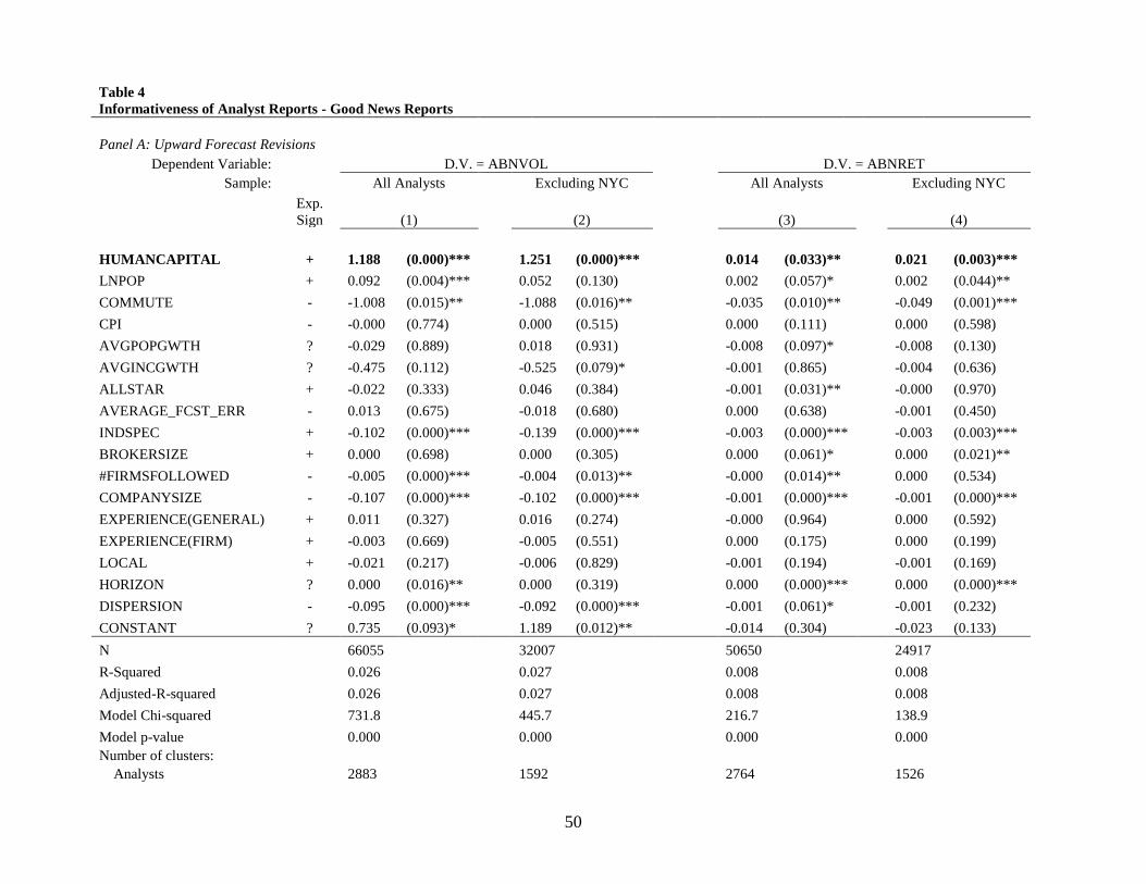
50

Table 4

Informativeness of Analyst Reports - Good News Reports

Panel A: Upward Forecast Revisions

Dependent Variable: D.V. = ABNVOL D.V. = ABNRET

Sample: All Analysts Excluding NYC All Analysts Excluding NYC

Exp.

Sign (1) (2) (3) (4)

HUMANCAPITAL + 1.188 (0.000)*** 1.251 (0.000)*** 0.014 (0.033)** 0.021 (0.003)***

LNPOP + 0.092 (0.004)*** 0.052 (0.130) 0.002 (0.057)* 0.002 (0.044)**

COMMUTE - -1.008 (0.015)** -1.088 (0.016)** -0.035 (0.010)** -0.049 (0.001)***

CPI - -0.000 (0.774) 0.000 (0.515) 0.000 (0.111) 0.000 (0.598)

AVGPOPGWTH ? -0.029 (0.889) 0.018 (0.931) -0.008 (0.097)* -0.008 (0.130)

AVGINCGWTH ? -0.475 (0.112) -0.525 (0.079)* -0.001 (0.865) -0.004 (0.636)

ALLSTAR + -0.022 (0.333) 0.046 (0.384) -0.001 (0.031)** -0.000 (0.970)

AVERAGE_FCST_ERR - 0.013 (0.675) -0.018 (0.680) 0.000 (0.638) -0.001 (0.450)

INDSPEC + -0.102 (0.000)*** -0.139 (0.000)*** -0.003 (0.000)*** -0.003 (0.003)***

BROKERSIZE + 0.000 (0.698) 0.000 (0.305) 0.000 (0.061)* 0.000 (0.021)**

#FIRMSFOLLOWED - -0.005 (0.000)*** -0.004 (0.013)** -0.000 (0.014)** 0.000 (0.534)

COMPANYSIZE - -0.107 (0.000)*** -0.102 (0.000)*** -0.001 (0.000)*** -0.001 (0.000)***

EXPERIENCE(GENERAL) + 0.011 (0.327) 0.016 (0.274) -0.000 (0.964) 0.000 (0.592)

EXPERIENCE(FIRM) + -0.003 (0.669) -0.005 (0.551) 0.000 (0.175) 0.000 (0.199)

LOCAL + -0.021 (0.217) -0.006 (0.829) -0.001 (0.194) -0.001 (0.169)

HORIZON ? 0.000 (0.016)** 0.000 (0.319) 0.000 (0.000)*** 0.000 (0.000)***

DISPERSION - -0.095 (0.000)*** -0.092 (0.000)*** -0.001 (0.061)* -0.001 (0.232)

CONSTANT ? 0.735 (0.093)* 1.189 (0.012)** -0.014 (0.304) -0.023 (0.133)

N 66055 32007 50650 24917

R-Squared 0.026 0.027 0.008 0.008

Adjusted-R-squared 0.026 0.027 0.008 0.008

Model Chi-squared 731.8 445.7 216.7 138.9

Model p-value 0.000 0.000 0.000 0.000

Number of clusters:

Analysts 2883 1592 2764 1526

51

Firms 4245 3718 3304 2887

(Table 4, cont.)

Panel B: Added to Buy List Recommendation Changes

Dependent Variable: D.V. = ABNVOL D.V. = ABNRET

Sample: All Analysts Excluding NYC All Analysts Excluding NYC

Exp.

Sign (1) (2) (3) (4)

HUMANCAPITAL + 1.646 (0.000)*** 1.572 (0.001)*** 0.033 (0.008)*** 0.041 (0.001)***

LNPOP + 0.198 (0.000)*** 0.154 (0.007)*** -0.002 (0.252) -0.000 (0.807)

COMMUTE - -2.127 (0.002)*** -2.018 (0.010)** -0.012 (0.620) -0.029 (0.226)

CPI - -0.004 (0.000)*** -0.003 (0.003)*** 0.000 (0.002)*** 0.000 (0.005)***

AVGPOPGWTH ? 0.137 (0.763) 0.056 (0.901) -0.005 (0.672) -0.013 (0.264)

AVGINCGWTH ? -0.862 (0.133) -0.737 (0.197) -0.004 (0.795) -0.007 (0.624)

ALLSTAR + -0.004 (0.934) 0.164 (0.331) 0.006 (0.300) -0.009 (0.020)**

AVERAGE_FCST_ERR - -0.103 (0.041)** -0.166 (0.017)** -0.005 (0.001)*** -0.003 (0.235)

INDSPEC + -0.088 (0.075)* -0.110 (0.088)* -0.001 (0.660) -0.003 (0.112)

BROKERSIZE + 0.002 (0.000)*** 0.002 (0.000)*** 0.000 (0.002)*** 0.000 (0.000)***

#FIRMSFOLLOWED - -0.010 (0.000)*** -0.014 (0.000)*** -0.000 (0.013)** -0.001 (0.000)***

COMPANYSIZE - -0.178 (0.000)*** -0.183 (0.000)*** -0.006 (0.000)*** -0.006 (0.000)***

EXPERIENCE(GENERAL) + 0.012 (0.285) -0.001 (0.950) 0.000 (0.302) 0.000 (0.968)

EXPERIENCE(FIRM) + 0.111 (0.000)*** 0.127 (0.000)*** 0.003 (0.000)*** 0.003 (0.000)***

LOCAL + -0.051 (0.188) -0.088 (0.115) -0.001 (0.576) -0.001 (0.485)

STRONGBUY + -0.047 (0.173) 0.090 (0.037)** 0.002 (0.068)* 0.005 (0.000)***

CONSTANT ? 0.364 (0.621) 0.769 (0.303) 0.063 (0.011)** 0.041 (0.088)*

N 18996 10364 19132 10422

R-Squared 0.063 0.070 0.042 0.072

Adjusted-R-squared 0.063 0.071 0.042 0.072

Model Chi-squared 917.1 646.5 720.8 495.8

Model p-value 0.000 0.000 0.000 0.000

Number of clusters:

Analysts 2683 1500 2688 1501

Firms 3352 2817 3370 2834

52

(Table 4, cont.)

This table presents the results of estimating Equations (3a) and (3b) for Upward Forecast Revisions in Panel A and for the Added to Buy List

sample in Panel B. The dependent variable is ABNVOL in columns (1) and (2) and ABNRET in columns (3) and (4) of each panel. All regressions

are run at the individual forecast/recommendation level. Columns (2) and (4) of each panel exclude forecasts/recommendations issued by analysts

located in New York. Only reports which update a previously issued forecast/recommendation from the same analyst for the same firm are

included, and only if the recommendation or forecast provided good news about the firm (i.e., added the firm to the analyst's buy list or revised

the analyst's earnings forecast upward). In the case of forecasts, the forecast revision must be updating a previously issued forecast for the same

fiscal year as well. The variable of interest is HUMANCAPITAL, the percentage of the population in the analyst's city with a bachelor's degree

or higher. Two-tailed p-values, based on robust standard errors and two-way clustering by firm and analyst, are presented in parentheses beside

the coefficient estimates. *, **, and *** indicate two-tailed statistical significance at p<0.10, p<0.05, and p<0.01, respectively. All variables are

defined in the text and Appendix A.

53

Table 5

Informativeness of Analyst Reports - Bad News Reports

Panel A: Downward Forecast Revisions

Dependent Variable: D.V. = ABNVOL D.V. = ABNRET

Sample: All Analysts Excluding NYC All Analysts Excluding NYC

Exp.

Sign (1) (2)

Exp.

Sign (3) (4)

HUMANCAPITAL + 1.765 (0.000)*** 1.707 (0.000)*** - -0.024 (0.000)*** -0.026 (0.000)***

LNPOP + 0.236 (0.000)*** 0.141 (0.001)*** - -0.001 (0.409) -0.000 (0.812)

COMMUTE - -2.696 (0.000)*** -2.318 (0.000)*** + 0.021 (0.088)* 0.026 (0.049)**

CPI - -0.002 (0.000)*** -0.001 (0.079)* + -0.000 (0.348) -0.000 (0.120)

AVGPOPGWTH ? -0.184 (0.402) -0.224 (0.317) ? 0.007 (0.164) 0.006 (0.242)

AVGINCGWTH ? -0.328 (0.275) -0.236 (0.440) ? 0.000 (0.965) -0.004 (0.659)

ALLSTAR + 0.012 (0.643) -0.040 (0.519) - 0.002 (0.146) 0.001 (0.555)

AVERAGE_FCST_ERR - 0.031 (0.369) -0.034 (0.487) + 0.001 (0.314) 0.001 (0.606)

INDSPEC + -0.060 (0.052)* -0.133 (0.002)*** - 0.002 (0.010)** 0.002 (0.132)

BROKERSIZE + 0.000 (0.717) 0.001 (0.036)** - -0.000 (0.054)* -0.000 (0.057)*

#FIRMSFOLLOWED - -0.003 (0.008)*** 0.000 (0.922) + 0.000 (0.030)** 0.000 (0.622)

COMPANYSIZE - -0.099 (0.000)*** -0.097 (0.000)*** + 0.002 (0.000)*** 0.002 (0.000)***

EXPERIENCE(GENERAL) + 0.014 (0.297) 0.020 (0.224) - 0.000 (0.792) -0.001 (0.188)

EXPERIENCE(FIRM) + -0.019 (0.014)** -0.024 (0.023)** - -0.000 (0.077)* -0.000 (0.327)

LOCAL + 0.010 (0.628) 0.014 (0.677) - 0.000 (0.881) 0.001 (0.095)*

HORIZON ? 0.001 (0.000)*** 0.001 (0.000)*** ? -0.000 (0.001)*** -0.000 (0.001)***

DISPERSION - -0.105 (0.000)*** -0.132 (0.000)*** + 0.001 (0.089)* 0.000 (0.920)

CONSTANT ? -0.964 (0.061)* 0.059 (0.912) ? -0.002 (0.848) -0.003 (0.819)

N 78453 38005 59352 29134

R-Squared 0.018 0.018 0.008 0.011

Adjusted-R-squared 0.018 0.018 0.008 0.011

Model Chi-squared 584.472 307.864 311.934 166.736

Model p-value 0.000 0.000 0.000 0.000

Number of clusters:

Analysts 2898 1598 2779 1536

Firms 4343 3799 3380 2943

54

(Table 5, cont.)

Panel B: Added to Hold/Sell List Recommendations

Dependent Variable: D.V. = ABNVOL D.V. = ABNRET

Sample: All Analysts Excluding NYC All Analysts Excluding NYC

Exp.

Sign (1) (2)

Exp.

Sign (3) (4)

HUMANCAPITAL + 3.277 (0.003)*** 3.069 (0.010)*** - -0.057 (0.006)*** -0.040 (0.072)*

LNPOP + 0.459 (0.001)*** 0.308 (0.044)** - 0.002 (0.580) 0.001 (0.682)

COMMUTE - -3.686 (0.035)** -2.605 (0.200) + 0.018 (0.624) -0.013 (0.763)

CPI - -0.008 (0.000)*** -0.005 (0.029)** + -0.000 (0.061)* -0.000 (0.051)*

AVGPOPGWTH ? 0.911 (0.420) 0.590 (0.606) ? 0.026 (0.209) 0.040 (0.061)*

AVGINCGWTH ? -2.464 (0.074)* -2.390 (0.063)* ? -0.003 (0.915) -0.008 (0.776)

ALLSTAR + 0.003 (0.981) -0.412 (0.151) - 0.001 (0.640) 0.011 (0.027)**

AVERAGE_FCST_ERR - -0.255 (0.052)* -0.121 (0.544) + 0.011 (0.000)*** 0.009 (0.023)**

INDSPEC + 0.002 (0.988) -0.150 (0.361) - 0.005 (0.059)* 0.008 (0.011)**

BROKERSIZE + -0.000 (0.859) 0.002 (0.322) - -0.000 (0.001)*** -0.000 (0.000)***

#FIRMSFOLLOWED - -0.036 (0.000)*** -0.062 (0.000)*** + 0.001 (0.000)*** 0.001 (0.000)***

COMPANYSIZE - -0.374 (0.000)*** -0.360 (0.000)*** + 0.006 (0.000)*** 0.006 (0.000)***

EXPERIENCE(GENERAL) + 0.314 (0.000)*** 0.340 (0.000)*** - -0.005 (0.000)*** -0.004 (0.007)***

EXPERIENCE(FIRM) + -0.141 (0.000)*** -0.158 (0.001)*** - 0.003 (0.002)*** 0.003 (0.006)***

LOCAL + 0.154 (0.149) 0.041 (0.785) - -0.001 (0.742) 0.001 (0.733)

SELL + 1.116 (0.003)*** 0.687 (0.062)* - -0.022 (0.001)*** -0.010 (0.194)

STRONGSELL + 0.131 (0.822) 1.152 (0.187) - -0.004 (0.718) -0.023 (0.172)

CONSTANT ? -1.469 (0.448) 0.294 (0.888) ? -0.062 (0.137) -0.069 (0.127)

N 13547 7339 13846 7504

R-Squared 0.046 0.041 0.034 0.034

Adjusted-R-squared 0.046 0.041 0.034 0.034

Model Chi-squared 272.519 180.575 283.023 171.646

Model p-value 0.000 0.000 0.000 0.000

Number of clusters:

Analysts 2313 1239 2323 1243

Firms 3181 2537 3236 2581

55

(Table 5, cont.)

This table presents the results of estimating Equations (3a) and (3b) for downward forecast revisions in Panel A and the Added to Hold/Sell List sample

in Panel B. The dependent variable is ABNVOL in columns (1) and (2) and ABNRET in columns (3) and (4) of each panel. All regressions are run at

the individual forecast/recommendation level. Columns (2) and (4) of each panel exclude forecasts/recommendations issued by analysts located in New

York. Only reports which update a previously issued forecast or recommendation from the same analyst for the same firm are included, and only if the

recommendation or forecast provided bad news about the firm (i.e., added the firm to the hold/sell list or revised the earnings forecast downward). In the

case of forecasts, the forecast revisions must be for the same fiscal year as well. The variable of interest is HUMANCAPITAL, the percentage of the

population in the analyst's city with a bachelor's degree or higher. Two-tailed p-values, based on robust standard errors and two-way clustering by firm

and analyst, are presented in parentheses beside the coefficient estimates. *, **, and *** indicate two-tailed statistical significance at the p<0.10, p<0.05,

and p<0.01, respectively.

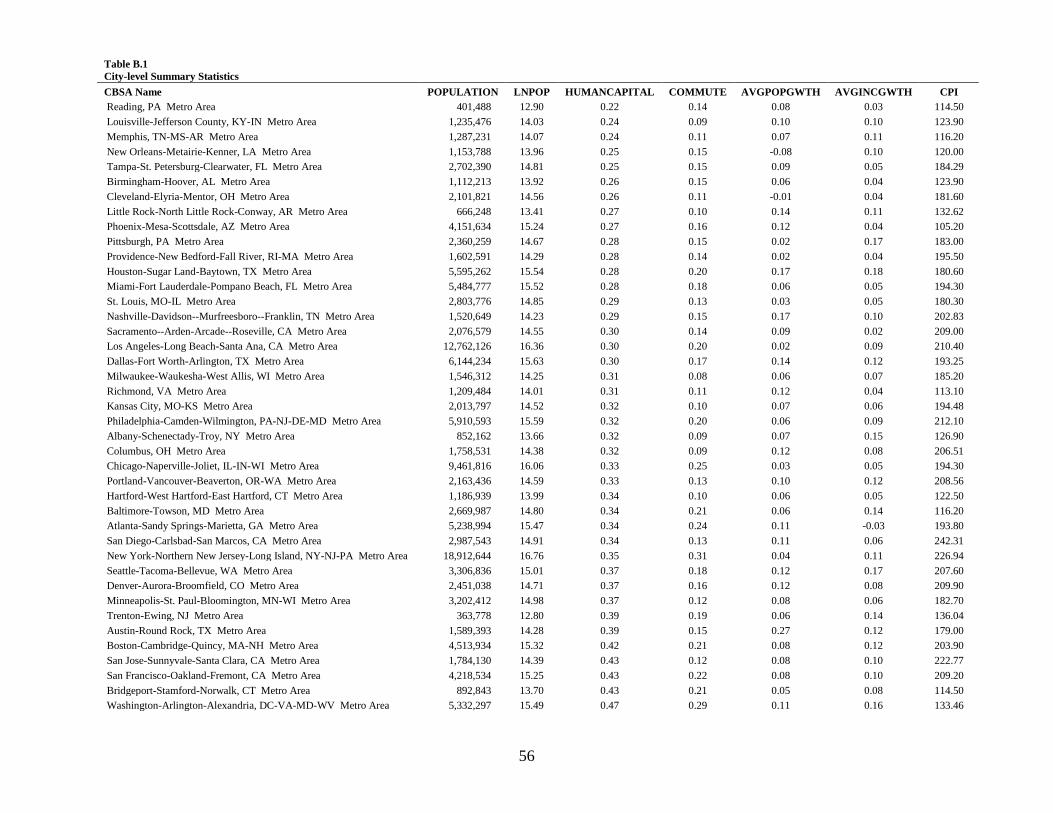
56

Table B.1

City-level Summary Statistics

CBSA Name POPULATION LNPOP HUMANCAPITAL COMMUTE AVGPOPGWTH AVGINCGWTH CPI

Reading, PA Metro Area 401,488 12.90 0.22 0.14 0.08 0.03 114.50

Louisville-Jefferson County, KY-IN Metro Area 1,235,476 14.03 0.24 0.09 0.10 0.10 123.90

Memphis, TN-MS-AR Metro Area 1,287,231 14.07 0.24 0.11 0.07 0.11 116.20

New Orleans-Metairie-Kenner, LA Metro Area 1,153,788 13.96 0.25 0.15 -0.08 0.10 120.00

Tampa-St. Petersburg-Clearwater, FL Metro Area 2,702,390 14.81 0.25 0.15 0.09 0.05 184.29

Birmingham-Hoover, AL Metro Area 1,112,213 13.92 0.26 0.15 0.06 0.04 123.90

Cleveland-Elyria-Mentor, OH Metro Area 2,101,821 14.56 0.26 0.11 -0.01 0.04 181.60

Little Rock-North Little Rock-Conway, AR Metro Area 666,248 13.41 0.27 0.10 0.14 0.11 132.62

Phoenix-Mesa-Scottsdale, AZ Metro Area 4,151,634 15.24 0.27 0.16 0.12 0.04 105.20

Pittsburgh, PA Metro Area 2,360,259 14.67 0.28 0.15 0.02 0.17 183.00

Providence-New Bedford-Fall River, RI-MA Metro Area 1,602,591 14.29 0.28 0.14 0.02 0.04 195.50

Houston-Sugar Land-Baytown, TX Metro Area 5,595,262 15.54 0.28 0.20 0.17 0.18 180.60

Miami-Fort Lauderdale-Pompano Beach, FL Metro Area 5,484,777 15.52 0.28 0.18 0.06 0.05 194.30

St. Louis, MO-IL Metro Area 2,803,776 14.85 0.29 0.13 0.03 0.05 180.30

Nashville-Davidson--Murfreesboro--Franklin, TN Metro Area 1,520,649 14.23 0.29 0.15 0.17 0.10 202.83

Sacramento--Arden-Arcade--Roseville, CA Metro Area 2,076,579 14.55 0.30 0.14 0.09 0.02 209.00

Los Angeles-Long Beach-Santa Ana, CA Metro Area 12,762,126 16.36 0.30 0.20 0.02 0.09 210.40

Dallas-Fort Worth-Arlington, TX Metro Area 6,144,234 15.63 0.30 0.17 0.14 0.12 193.25

Milwaukee-Waukesha-West Allis, WI Metro Area 1,546,312 14.25 0.31 0.08 0.06 0.07 185.20

Richmond, VA Metro Area 1,209,484 14.01 0.31 0.11 0.12 0.04 113.10

Kansas City, MO-KS Metro Area 2,013,797 14.52 0.32 0.10 0.07 0.06 194.48

Philadelphia-Camden-Wilmington, PA-NJ-DE-MD Metro Area 5,910,593 15.59 0.32 0.20 0.06 0.09 212.10

Albany-Schenectady-Troy, NY Metro Area 852,162 13.66 0.32 0.09 0.07 0.15 126.90

Columbus, OH Metro Area 1,758,531 14.38 0.32 0.09 0.12 0.08 206.51

Chicago-Naperville-Joliet, IL-IN-WI Metro Area 9,461,816 16.06 0.33 0.25 0.03 0.05 194.30

Portland-Vancouver-Beaverton, OR-WA Metro Area 2,163,436 14.59 0.33 0.13 0.10 0.12 208.56

Hartford-West Hartford-East Hartford, CT Metro Area 1,186,939 13.99 0.34 0.10 0.06 0.05 122.50

Baltimore-Towson, MD Metro Area 2,669,987 14.80 0.34 0.21 0.06 0.14 116.20

Atlanta-Sandy Springs-Marietta, GA Metro Area 5,238,994 15.47 0.34 0.24 0.11 -0.03 193.80

San Diego-Carlsbad-San Marcos, CA Metro Area 2,987,543 14.91 0.34 0.13 0.11 0.06 242.31

New York-Northern New Jersey-Long Island, NY-NJ-PA Metro Area 18,912,644 16.76 0.35 0.31 0.04 0.11 226.94

Seattle-Tacoma-Bellevue, WA Metro Area 3,306,836 15.01 0.37 0.18 0.12 0.17 207.60

Denver-Aurora-Broomfield, CO Metro Area 2,451,038 14.71 0.37 0.16 0.12 0.08 209.90

Minneapolis-St. Paul-Bloomington, MN-WI Metro Area 3,202,412 14.98 0.37 0.12 0.08 0.06 182.70

Trenton-Ewing, NJ Metro Area 363,778 12.80 0.39 0.19 0.06 0.14 136.04

Austin-Round Rock, TX Metro Area 1,589,393 14.28 0.39 0.15 0.27 0.12 179.00

Boston-Cambridge-Quincy, MA-NH Metro Area 4,513,934 15.32 0.42 0.21 0.08 0.12 203.90

San Jose-Sunnyvale-Santa Clara, CA Metro Area 1,784,130 14.39 0.43 0.12 0.08 0.10 222.77

San Francisco-Oakland-Fremont, CA Metro Area 4,218,534 15.25 0.43 0.22 0.08 0.10 209.20

Bridgeport-Stamford-Norwalk, CT Metro Area 892,843 13.70 0.43 0.21 0.05 0.08 114.50

Washington-Arlington-Alexandria, DC-VA-MD-WV Metro Area 5,332,297 15.49 0.47 0.29 0.11 0.16 133.46

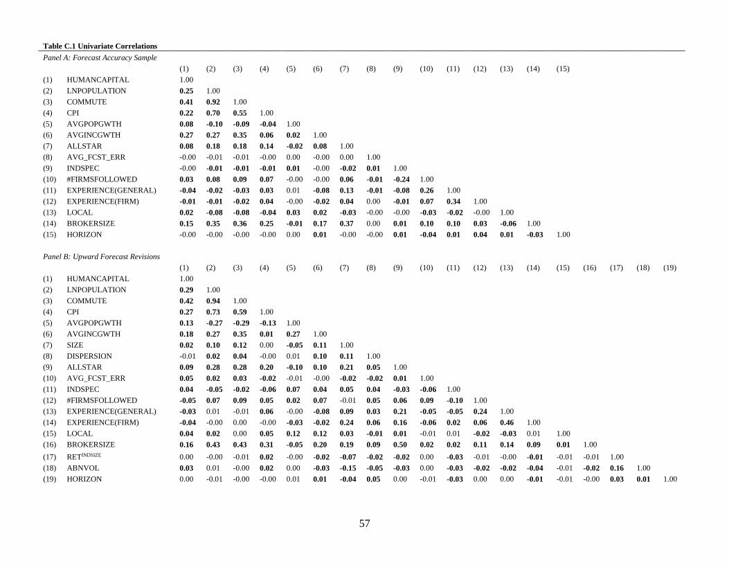
57

Table C.1 Univariate Correlations

Panel A: Forecast Accuracy Sample

(1) (2) (3) (4) (5) (6) (7) (8) (9) (10) (11) (12) (13) (14) (15)

(1) HUMANCAPITAL 1.00

(2) LNPOPULATION 0.25 1.00

(3) COMMUTE 0.41 0.92 1.00

(4) CPI 0.22 0.70 0.55 1.00

(5) AVGPOPGWTH 0.08 -0.10 -0.09 -0.04 1.00

(6) AVGINCGWTH 0.27 0.27 0.35 0.06 0.02 1.00

(7) ALLSTAR 0.08 0.18 0.18 0.14 -0.02 0.08 1.00

(8) AVG_FCST_ERR -0.00 -0.01 -0.01 -0.00 0.00 -0.00 0.00 1.00

(9) INDSPEC -0.00 -0.01 -0.01 -0.01 0.01 -0.00 -0.02 0.01 1.00

(10) #FIRMSFOLLOWED 0.03 0.08 0.09 0.07 -0.00 -0.00 0.06 -0.01 -0.24 1.00

(11) EXPERIENCE(GENERAL) -0.04 -0.02 -0.03 0.03 0.01 -0.08 0.13 -0.01 -0.08 0.26 1.00

(12) EXPERIENCE(FIRM) -0.01 -0.01 -0.02 0.04 -0.00 -0.02 0.04 0.00 -0.01 0.07 0.34 1.00

(13) LOCAL 0.02 -0.08 -0.08 -0.04 0.03 0.02 -0.03 -0.00 -0.00 -0.03 -0.02 -0.00 1.00

(14) BROKERSIZE 0.15 0.35 0.36 0.25 -0.01 0.17 0.37 0.00 0.01 0.10 0.10 0.03 -0.06 1.00

(15) HORIZON -0.00 -0.00 -0.00 -0.00 0.00 0.01 -0.00 -0.00 0.01 -0.04 0.01 0.04 0.01 -0.03 1.00

Panel B: Upward Forecast Revisions

(1) (2) (3) (4) (5) (6) (7) (8) (9) (10) (11) (12) (13) (14) (15) (16) (17) (18) (19)

(1) HUMANCAPITAL 1.00

(2) LNPOPULATION 0.29 1.00

(3) COMMUTE 0.42 0.94 1.00

(4) CPI 0.27 0.73 0.59 1.00

(5) AVGPOPGWTH 0.13 -0.27 -0.29 -0.13 1.00

(6) AVGINCGWTH 0.18 0.27 0.35 0.01 0.27 1.00

(7) SIZE 0.02 0.10 0.12 0.00 -0.05 0.11 1.00

(8) DISPERSION -0.01 0.02 0.04 -0.00 0.01 0.10 0.11 1.00

(9) ALLSTAR 0.09 0.28 0.28 0.20 -0.10 0.10 0.21 0.05 1.00

(10) AVG_FCST_ERR 0.05 0.02 0.03 -0.02 -0.01 -0.00 -0.02 -0.02 0.01 1.00

(11) INDSPEC 0.04 -0.05 -0.02 -0.06 0.07 0.04 0.05 0.04 -0.03 -0.06 1.00

(12) #FIRMSFOLLOWED -0.05 0.07 0.09 0.05 0.02 0.07 -0.01 0.05 0.06 0.09 -0.10 1.00

(13) EXPERIENCE(GENERAL) -0.03 0.01 -0.01 0.06 -0.00 -0.08 0.09 0.03 0.21 -0.05 -0.05 0.24 1.00

(14) EXPERIENCE(FIRM) -0.04 -0.00 0.00 -0.00 -0.03 -0.02 0.24 0.06 0.16 -0.06 0.02 0.06 0.46 1.00

(15) LOCAL 0.04 0.02 0.00 0.05 0.12 0.12 0.03 -0.01 0.01 -0.01 0.01 -0.02 -0.03 0.01 1.00

(16) BROKERSIZE 0.16 0.43 0.43 0.31 -0.05 0.20 0.19 0.09 0.50 0.02 0.02 0.11 0.14 0.09 0.01 1.00

(17) RETINDSIZE 0.00 -0.00 -0.01 0.02 -0.00 -0.02 -0.07 -0.02 -0.02 0.00 -0.03 -0.01 -0.00 -0.01 -0.01 -0.01 1.00

(18) ABNVOL 0.03 0.01 -0.00 0.02 0.00 -0.03 -0.15 -0.05 -0.03 0.00 -0.03 -0.02 -0.02 -0.04 -0.01 -0.02 0.16 1.00

(19) HORIZON 0.00 -0.01 -0.00 -0.00 0.01 0.01 -0.04 0.05 0.00 -0.01 -0.03 0.00 0.00 -0.01 -0.01 -0.00 0.03 0.01 1.00

58

(Table C.1, cont.)

Panel C: Downward Forecast Revisions

(1) (2) (3) (4) (5) (6) (7) (8) (9) (10) (11) (12) (13) (14) (15) (16) (17) (18) (19)

(1) HUMANCAPITAL 1.00

(2) LNPOPULATION 0.30 1.00

(3) COMMUTE 0.43 0.94 1.00

(4) CPI 0.25 0.73 0.60 1.00

(5) AVGPOPGWTH 0.09 -0.34 -0.33 -0.20 1.00

(6) AVGINCGWTH 0.22 0.29 0.37 0.04 0.21 1.00

(7) SIZE 0.03 0.10 0.12 0.02 -0.04 0.12 1.00

(8) DISPERSION 0.01 0.02 0.04 0.02 0.01 0.06 0.05 1.00

(9) ALLSTAR 0.09 0.28 0.28 0.20 -0.12 0.09 0.23 0.04 1.00

(10) AVG_FCST_ERR 0.04 0.03 0.04 -0.01 -0.02 -0.01 -0.03 -0.02 0.01 1.00

(11) INDSPEC 0.04 -0.05 -0.02 -0.05 0.08 0.01 0.05 0.02 -0.04 -0.06 1.00

(12) #FIRMSFOLLOWED -0.03 0.07 0.08 0.05 0.01 0.03 0.01 0.06 0.07 0.07 -0.10 1.00

(13) EXPERIENCE(GENERAL) -0.03 -0.01 -0.02 0.02 -0.01 -0.09 0.11 0.03 0.21 -0.03 -0.06 0.25 1.00

(14) EXPERIENCE(FIRM) -0.04 -0.03 -0.02 -0.01 -0.01 -0.05 0.21 0.05 0.16 -0.05 0.00 0.06 0.47 1.00

(15) LOCAL 0.04 0.03 0.01 0.05 0.11 0.12 0.04 -0.02 0.01 -0.01 -0.00 -0.02 -0.01 0.02 1.00

(16) BROKERSIZE 0.17 0.43 0.44 0.31 -0.11 0.20 0.22 0.08 0.51 0.02 -0.00 0.11 0.12 0.07 0.01 1.00

(17) RETINDSIZE -0.01 0.00 0.01 -0.01 -0.00 0.01 0.08 0.01 0.02 0.00 0.02 0.01 0.01 0.01 0.00 0.01 1.00

(18) ABNVOL 0.02 -0.01 -0.01 -0.00 0.00 -0.02 -0.12 -0.04 -0.02 0.01 -0.02 -0.02 -0.01 -0.04 0.00 -0.03 -0.19 1.00

(19) HORIZON 0.01 -0.00 -0.01 0.00 0.00 -0.01 -0.05 0.03 -0.00 0.01 -0.02 0.01 0.00 -0.02 0.00 -0.00 -0.02 0.04 1.00

Panel D: Added to Buy Recommendations

(1) (2) (3) (4) (5) (6) (7) (8) (9) (10) (11) (12) (13) (14) (15) (16) (17)

(1) HUMANCAPITAL 1.00

(2) LNPOPULATION 0.21 1.00

(3) COMMUTE 0.35 0.93 1.00

(4) CPI 0.24 0.67 0.52 1.00

(5) AVGPOPGWTH 0.15 -0.45 -0.39 -0.24 1.00

(6) AVGINCGWTH 0.31 0.29 0.41 0.04 0.09 1.00

(7) SIZE 0.02 0.11 0.14 0.03 -0.06 0.10 1.00

(8) ALLSTAR 0.06 0.23 0.23 0.16 -0.11 0.09 0.21 1.00

(9) AVG_FCST_ERR 0.01 0.06 0.08 0.01 -0.02 0.05 -0.01 0.03 1.00

(10) INDSPEC 0.03 -0.02 0.01 -0.03 0.03 -0.02 0.06 0.01 -0.06 1.00

(11) #FIRMSFOLLOWED 0.03 0.11 0.12 0.09 -0.06 0.05 0.09 -0.00 0.01 -0.20 1.00

(12) EXPERIENCE(GENERAL) -0.01 -0.05 -0.05 -0.01 0.05 -0.05 0.08 0.14 -0.10 -0.03 0.11 1.00

(13) EXPERIENCE(FIRM) -0.02 0.01 0.03 -0.01 -0.01 0.00 0.19 0.14 -0.06 0.05 0.08 0.32 1.00

(14) LOCAL 0.10 0.00 0.01 0.04 0.07 0.08 0.03 0.01 -0.01 -0.00 -0.01 0.00 0.03 1.00

(15) BROKERSIZE 0.10 0.32 0.34 0.18 -0.08 0.15 0.24 0.46 0.03 0.07 -0.02 0.14 0.12 0.00 1.00

(16) RETINDSIZE 0.02 -0.01 -0.02 0.02 0.02 -0.02 -0.13 0.02 -0.03 0.00 -0.03 0.05 0.11 -0.00 0.02 1.00

(17) ABNVOL 0.01 -0.03 -0.03 -0.04 0.02 -0.03 -0.13 0.00 -0.03 -0.00 -0.05 0.06 0.17 -0.01 0.01 0.27 1.00

59

(Table C.1, cont.)

Panel E: Added to Hold/Sell Recommendations

(1) (2) (3) (4) (5) (6) (7) (8) (9) (10) (11) (12) (13) (14) (15) (16) (17)

(1) HUMANCAPITAL 1.00

(2) LNPOPULATION 0.23 1.00

(3) COMMUTE 0.38 0.93 1.00

(4) CPI 0.21 0.67 0.52 1.00

(5) AVGPOPGWTH 0.15 -0.47 -0.39 -0.27 1.00

(6) AVGINCGWTH 0.35 0.30 0.41 0.05 0.07 1.00

(7) SIZE 0.04 0.13 0.16 0.03 -0.08 0.10 1.00

(8) ALLSTAR 0.07 0.24 0.24 0.16 -0.12 0.10 0.22 1.00

(9) AVG_FCST_ERR 0.01 0.06 0.08 -0.00 -0.01 0.05 0.01 0.03 1.00

(10) INDSPEC 0.04 -0.01 0.02 -0.04 0.04 -0.01 0.08 0.03 -0.07 1.00

(11) #FIRMSFOLLOWED 0.04 0.11 0.11 0.10 -0.06 0.02 0.06 -0.02 -0.01 -0.17 1.00

(12) EXPERIENCE(GENERAL) -0.05 -0.09 -0.09 -0.03 0.05 -0.11 0.10 0.17 -0.06 -0.00 0.04 1.00

(13) EXPERIENCE(FIRM) -0.05 -0.03 -0.01 -0.02 -0.01 -0.05 0.22 0.17 -0.06 0.04 0.01 0.48 1.00

(14) LOCAL 0.09 0.01 0.01 0.05 0.05 0.07 0.02 0.00 -0.01 -0.01 -0.02 -0.02 0.01 1.00

(15) BROKERSIZE 0.09 0.32 0.34 0.18 -0.09 0.15 0.22 0.47 0.04 0.08 -0.07 0.12 0.10 0.01 1.00

(16) RETINDSIZE -0.02 0.02 0.03 -0.01 -0.02 0.01 0.15 0.02 0.04 0.02 0.06 -0.02 0.04 -0.00 0.00 1.00

(17) ABNVOL 0.01 -0.03 -0.04 -0.03 0.03 -0.03 -0.18 -0.03 -0.02 -0.00 -0.08 0.02 -0.05 0.01 -0.03 -0.40 1.00

The table presents univariate correlations between selected regression variables. Bold test indicates significance at p<0.01. All variables are defined in the text and in Appendix B.

60

0

50

100

150

200

250

300

350R

eadin

g, P

A

Lo

uis

vil

le,

KY

Mem

phis

, T

N

New

Orl

ean

s, L

A

Tam

pa,

FL

Bir

min

gh

am,

AL

Cle

vel

and

, O

H

Lit

tle

Ro

ck,

AR

Ph

oen

ix,

AZ

Pit

tsb

urg

h, P

A

Pro

vid

ence

, R

I

Ho

ust

on,

TX

Mia

mi,

FL

St.

Lo

uis

, M

O

Nas

hv

ille

, T

N

Sac

ram

ento

, C

A

Lo

s A

ngel

es,

CA

Dal

las,

TX

Mil

wau

kee

, W

I

Ric

hm

on

d,

VA

Kan

sas

Cit

y,

MO

Ph

ilad

elp

hia

, P

A

Alb

any,

NY

Colu

mb

us,

OH

Chic

ago

, IL

Po

rtla

nd,

OR

Har

tfo

rd,

CT

Bal

tim

ore

, M

D

Atl

anta

, G

A

San

Die

go

, C

A

New

Yo

rk,

NY

Sea

ttle

, W

A

Den

ver

, C

O

Min

nea

po

lis,

MN

Tre

nto

n,

NJ

Au

stin

, T

X

Bost

on,

MA

San

Jo

se,

CA

San

Fra

nci

sco

, C

A

Bri

dg

eport

, C

T

Was

hin

gto

n, D

C

Figure 1: Number of Analysts by City, sorted by HUMANCAPITAL

High Human CapitalLow Human Capital

61

0

50

100

150

200

250

300

350

Tre

nto

n,

NJ

Rea

din

g, P

A

Lit

tle

Ro

ck,

AR

Alb

any,

NY

Bri

dg

eport

, C

T

Bir

min

gh

am,

AL

New

Orl

ean

s, L

A

Har

tfo

rd,

CT

Ric

hm

on

d,

VA

Lo

uis

vil

le,

KY

Mem

phis

, T

N

Nas

hv

ille

, T

N

Mil

wau

kee

, W

I

Au

stin

, T

X

Pro

vid

ence

, R

I

Colu

mb

us,

OH

San

Jo

se,

CA

Kan

sas

Cit

y,

MO

Sac

ram

ento

, C

A

Cle

vel

and

, O

H

Po

rtla

nd,

OR

Pit

tsb

urg

h, P

A

Den

ver

, C

O

Bal

tim

ore

, M

D

Tam

pa,

FL

St.

Lo

uis

, M

O

San

Die

go

, C

A

Min

nea

po

lis,

MN

Sea

ttle

, W

A

Ph

oen

ix,

AZ

San

Fra

nci

sco

, C

A

Bost

on,

MA

Atl

anta

, G

A

Was

hin

gto

n, D

C

Mia

mi,

FL

Ho

ust

on,

TX

Ph

ilad

elp

hia

, P

A

Dal

las,

TX

Chic

ago

, IL

Lo

s A

ngel

es,

CA

New

Yo

rk,

NY

Figure 2: Number of Analysts by City, sorted by POPULATION

High PopulationLow Population

62

Figure 3: Average Abnormal Trading Volume and Unexpected Returns: Good News Reports

0.00

0.00

0.00

0.00

0.00

0.01

0.01

0.01

0.01

0.01

0.02

0.02

-20

-18

-16

-14

-12

-10 -8 -6 -4 -2 0 2 4 6 8

10

12

14

16

18

20

Ind

ust

ry-S

ize

Ad

just

ed

Re

turn

Day

Panel B: Upward Forecast Revisions:

Unexpected Returns

Quintile 1 Quintile 5

0.9

1.1

1.3

1.5

1.7

1.9

2.1

2.3

-20

-18

-16

-14

-12

-10 -8 -6 -4 -2 0 2 4 6 8

10

12

14

16

18

20

Ab

no

rma

l V

olu

me

Day

Panel A: Upward Forecast Revisions:

Abnormal Volume

Quintile 1 Quintile 5

-0.01

0.00

0.01

0.01

0.02

0.02

0.03

0.03

0.04

-20

-18

-16

-14

-12

-10 -8 -6 -4 -2 0 2 4 6 8

10

12

14

16

18

20

Ind

ust

ry-S

ize

Ad

just

ed R

etu

rn

Day

Panel D: Added to Buy Recommendations:

Unexpected Returns

Quintile 1 Quintile 5

0.9

1.1

1.3

1.5

1.7

1.9

2.1

-20

-18

-16

-14

-12

-10 -8 -6 -4 -2 0 2 4 6 8

10

12

14

16

18

20

Ab

no

rma

l V

olu

me

Day

Panel C: Added to Buy Recommendations:

Abnormal Volume

Quintile 1 Quintile 5

63

Figure 4: Average Abnormal Trading Volume and Unexpected Returns: Bad News Reports

-0.02

-0.01

-0.01

-0.01

-0.01

-0.01

0.00

0.00

0.00

0.00

-20 -17 -14 -11 -8 -5 -2 1 4 7 10 13 16 19

Ind

ust

ry-S

ize

Ad

just

ed R

etu

rn

Day

Panel B: Downward Forecast Revisions:

Unexpected Returns

Quintile 1 Quintile 5

0.8

1.0

1.2

1.4

1.6

1.8

2.0

2.2

2.4

2.6

-20

-18

-16

-14

-12

-10 -8 -6 -4 -2 0 2 4 6 8

10

12

14

16

18

20

Ab

no

rma

l V

olu

me

Day

Panel A: Downward Forecast Revisions:

Abnormal Volume

Quintile 1 Quintile 5

-0.06

-0.05

-0.04

-0.03

-0.02

-0.01

0.01

-20

-18

-16

-14

-12

-10 -8 -6 -4 -2 0 2 4 6 8

10

12

14

16

18

20

Ind

ust

ry-S

ize

Ad

just

ed R

etu

rn

Day

Panel D: Added to Hold/Sell Recommendations:

Unexpected Returns

Quintile 1 Quintile 5

0.8

1.3

1.8

2.3

2.8

3.3

3.8

-20

-18

-16

-14

-12

-10 -8 -6 -4 -2 0 2 4 6 8

10

12

14

16

18

20

Ab

no

rma

l V

olu

me

Day

Panel C: Added to Hold/Sell Recommendations:

Abnormal Volume

Quintile 1 Quintile 5