City of Cupertino, CA | Home

City of Cupertino 2015 Community-wide and Municipal Operations Greenhouse Gas Emissions Inventory Report

January 2018

i

Acknowledgements This 2015 Community-wide and Municipal Operations Greenhouse Gas Emissions Inventory Report was developed for the City of Cupertino Office of the City Manager. The community-wide inventory was developed using the Global Protocol for Community-Scale Greenhouse Gas Emission Inventories (GPC) and the municipal operations inventory was developed using the Local Government Operations Protocol (LGO). These inventories are intended to assist the City of Cupertino in tracking progress towards the City’s emissions reduction goals established in the City of Cupertino Climate Action Plan (2015). Project Consultant: Betty Seto, Ben Butterworth (DNV GL) Cupertino City Staff: Misty Mersich, Gilee Corral

1

Table of Contents

Table of Contents

1. INTRODUCTION ................................................................................................................ 2 1.1 2015 Community-wide Emissions Inventory ......................................................... 2

1.1.1 Summary of Community-wide Emissions Inventory Results...................................... 2 1.1.2 Energy Sector ................................................................................................................ 5 1.1.3 Transportation Sector ................................................................................................... 7 1.1.4 Off-road Sector ............................................................................................................. 8 1.1.5 Solid Waste Sector ....................................................................................................... 8 1.1.6 Wastewater Sector ....................................................................................................... 9

1.2 2015 Municipal Operations Emissions Inventory ................................................. 10 1.1.7 Summary of Municipal Operations Emissions Inventory Results ............................. 10 1.1.8 Facilities Sector ........................................................................................................... 13 1.1.9 Vehicle Fleet Sector ..................................................................................................... 13 1.1.10 Solid Waste Sector ...................................................................................................... 14 1.1.11 Water Services Sector ................................................................................................. 14

1.3 2015 – 2050 Community-wide Emissions Forecast .............................................. 16 1.4 Community-wide Inventory Methodology ........................................................... 20

1.1.12 Stationary Energy ...................................................................................................... 20 1.1.13 Transportation ........................................................................................................... 24 1.1.14 Waste .......................................................................................................................... 26

1.5 Municipal Operations Inventory Methodology .................................................... 28 1.1.15 Facilities ..................................................................................................................... 28 1.1.16 Water Services............................................................................................................ 29 1.1.17 Vehicle Fleet ............................................................................................................... 30 1.1.18 Solid Waste ................................................................................................................ 30

1.6 2015-2050 Community-wide Emissions Forecast Methodology ......................... 32 1.1.19 Business-as-usual Forecast Without State Measures ................................................ 32 1.1.20 Business-as-usual Forecast With State Measures ..................................................... 32

1.7 Adjustments to 2010 Baseline Inventories ............................................................ 35 1.1.21 Adjustments to the 2010 Community-wide Inventory ............................................... 35 1.1.22 Adjustments to the 2010 Municipal Operations Inventory ....................................... 38

2

1. INTRODUCTION

The City of Cupertino is pleased to present the 2015 community-wide and municipal operations

greenhouse gas (GHG) emissions inventories. Emissions inventories are developed to help

community and government leaders understand how GHG emissions are generated from various

activities in the community. Emissions accounting standards and protocols are used to assist cities

in compiling emissions data at both the community-wide scale and at the municipal operations

scale.

Cupertino established a baseline community-wide inventory and municipal operations inventory

for calendar year 2010 as part of the 2015 Climate Action Plan (CAP) process. This 2015 inventory

was developed to help the City track progress towards achieving emissions reduction goals

established in the CAP. The results of this inventory will be used to help forecast and assess

potential trends in emissions from 2015 to 2020, 2035 and 2050, and to determine if the City is

on track to meet its GHG reduction targets.

The community-wide inventory follows the Global Protocol for Community-Scale Greenhouse

Gas Emission Inventories (GPC) developed by the World Resources Institute, C40 Cities, and

ICLEI Local Governments for Sustainability. The GPC is the required protocol for The Global

Covenant of Mayors for Climate and Energy (Global Covenant)1, of which Cupertino is a member.

The municipal operations inventory follows the Local Government Operations Protocol (LGO)

developed by the California Air Resources Board, California Climate Action Registry, ICLEI and

the Climate Registry. Calendar year 2015 was chosen as the year for this inventory because it was

the most recent calendar year with complete data available.

1.1 2015 Community-wide Emissions Inventory 1.1.1 Summary of Community-wide Emissions Inventory Results

Our findings indicate that Cupertino emitted community-wide emissions of 294,281 metric tons

of carbon dioxide equivalent (MTCO2e) in 2015 from the energy, transportation, off-road sources,

1 The Global Covenant of Mayor’s for Climate and Energy is the new designation for the Compact of Mayors. The Compact of Mayors was launched by UN Secretary, C40 Cities Climate Leadership Group (C40), ICLEI – Local Governments for Sustainability (ICLEI) and the United Cities and Local Governments (UCLG) –with support from UN-Habitat, the UN’s lead agency on urban issues.

3

solid waste and wastewater sectors.2 This represents a 13.1% decrease from 2010 community-wide

emissions of 338,673 MTCO2e. Figure 1 and Table 1 provide a comparison of 2010 and 2015

community-wide emissions and trends by sector and subsector.

Figure 1: Cupertino community-wide emissions by sector – 2010 vs. 2015

2 Carbon dioxide equivalent (CO2e) is a unit of measure that normalizes the varying climate warming potencies of all six GHG emissions, which are carbon dioxide (CO2), methane (CH4), nitrous oxide (N2O), hydrofluorocarbons (HFCs), perfluorocarbons (PFCs), and sulfur hexafluoride (SF6). For example, one metric ton of methane is equivalent to 28 metric tons of CO2e. One metric ton of nitrous oxide is 265 metric tons of CO2e.

4

Table 1: Cupertino community-wide emissions by sector & subsector – 2010 vs. 2015

Table 2 provides a sector-by-sector analysis of key factors driving trends in community-wide emissions from 2010-2015.

Table 2: Summary of key 2010-2015 community-wide emissions trends

Emissions Sector Summary of 2010-2015 Trends

Energy

Energy emissions decreased 26% from 2010 to 2015. This trend in the energy sector is largely driven by a 47% decrease in commercial electricity emissions. Apple’s campus, which consumes a large portion of total commercial grid electricity in Cupertino and sources 100% of their electricity from renewable sources, is a major contributing factor to this decrease in emissions.

Transportation Transportation emissions increased 1% from 2010 to 2015. Improvements in on-road vehicle fuel efficiency were offset by a 6% increase the total vehicle miles travelled (VMT).

Off-Road Sources Off-road emissions increased 3% from 2010 to 2015. Modest increases in off-road emissions associated with construction and industrial equipment, which make up the majority of off-road emissions, drove the increase.

Solid Waste Solid waste emissions increased 20% from 2010 to 2015. A 20% increase in the amount of waste sent to landfills drove the increase in emissions.

Wastewater

Wastewater emissions decreased 23% from 2010 to 2015. This decrease is driven by a 26% decrease in the biochemical oxygen demand (BOD) treated per day at the San José-Santa Clara Regional Wastewater Facility. 4.3% of the total plant emissions were allocated to Cupertino based on population served.

3 The “Non-residential” subsector includes commercial, industrial, municipal and institutional customers. For electricity, this also includes direct access customers – a retail electric service where customers purchase electricity from a competitive provider called an Electric Service Provider (ESP), instead of from a regulated electric utility.

Sector/Subsector 2010

Emissions (MT CO2e/yr)

2015 Emissions

(MT CO2e/yr)

Percent Change

Energy 172,289 128,266 -26% Electricity Subtotal 85,451 54,318 -36%

Residential 25,427 22,396 -12% Non-residential3 60,025 31,922 -47%

Natural Gas Subtotal 86,837 73,948 -15% Residential 49,986 40,594 -19% Non-residential3 34,109 31,012 -9%

Fugitive Nat. Gas 2,742 2,342 -15% Transportation 104,112 105,225 +1% Off-Road Sources 24,496 25,165 +3% Solid Waste 15,185 18,219 +20% Wastewater 22,591 17,405 -23% Total 338,673 294,281 -13.1%

5

Figure 2 displays the relative contribution of each sector to overall 2015 community-wide emissions.

Figure 2: Cupertino 2015 community-wide emissions by sector

Energy (43.6%) and transportation (35.8%) continue to make up the vast majority of community-

wide emissions in Cupertino. Off-road sources (8.6%), solid waste (6.2%) and wastewater (5.9%)

make up the remaining community-wide emissions.

1.1.2 Energy Sector

As summarized in Table 3 below, community-wide emissions in the energy sector decreased 26%

from 2010 to 2015. The energy sector made up 43.6% of Cupertino’s total community-wide

emissions in 2015.

43.6%

35.8%

8.6%

6.2%5.9%

Energy

Transportation

Off-Road Sources

Solid Waste

Wastewater

6

Table 3: Cupertino community-wide energy sector consumption and emissions by fuel type – 2010 vs. 2015

The overall decrease in energy sector emissions was driven by a 36% decrease in total electricity emissions and a 15% decrease in natural gas emissions.

As summarized in Table 4 below, community-wide electricity emissions decreased 36% from 2010 to 2015. Electricity emissions made up 19% of Cupertino’s total community-wide emissions in 2015.

Table 4: Cupertino community-wide electricity consumption and emissions by subsector – 2010 vs. 2015

Total residential electricity consumption decreased 10% and total residential electricity emissions

decreased 12%. Residential electricity emissions decreased at a greater rate than residential

electricity consumption due to a lower emission factor associated with PG&E grid electricity. Total

non-residential electricity consumption increased 2%, but total non-residential electricity

emissions decreased 47%. Non-residential electricity emissions decreased substantially despite

an increase in non-residential electricity consumption due to a lower emission factor associated

Category

2010 Consumption (kWh or

therms)

2015 Consumption

(kWh or therms)

2010 Emissions (MT CO2e)


% Change Consump.

% Change Emissi

ons Electricity 409,319,124 404,190,175 85,451 54,318 -1% -36%

Natural Gas 15,805,499 13,498,530 84,095 71,606 -15% -15% Nat. Gas Fugitive 2,742 2,342 -15%

Total 172,289 128,266 -26%

Category

2010 Electricity

Consumption (kWh)

2015 Electricity

Consumption (kWh)

2010 Electricity Emissions (MT CO2e)

2015 Electricity Emissions (MT CO2e)

% Change Consump.

% Change Emissions

Residential 124,926,651 112,974,425 25,427 23,396 -10% -12%

Non-Residential 284,392,473 291,215,750 60,025 31,935 +2% -47%

PG&E Non-Residential 274,446,308 123,878,787 55,859 24,557 -55% -56%

Direct Access Non-Residential 9,946,165 167,336,963 4,166 7,377 +1,582% +77%

Total 409,319,124 404,190,175 85,451 54,318 -1% -36%

7

with PG&E grid electricity and large, non-residential electricity consumers switching to low

emissions direct access electricity.

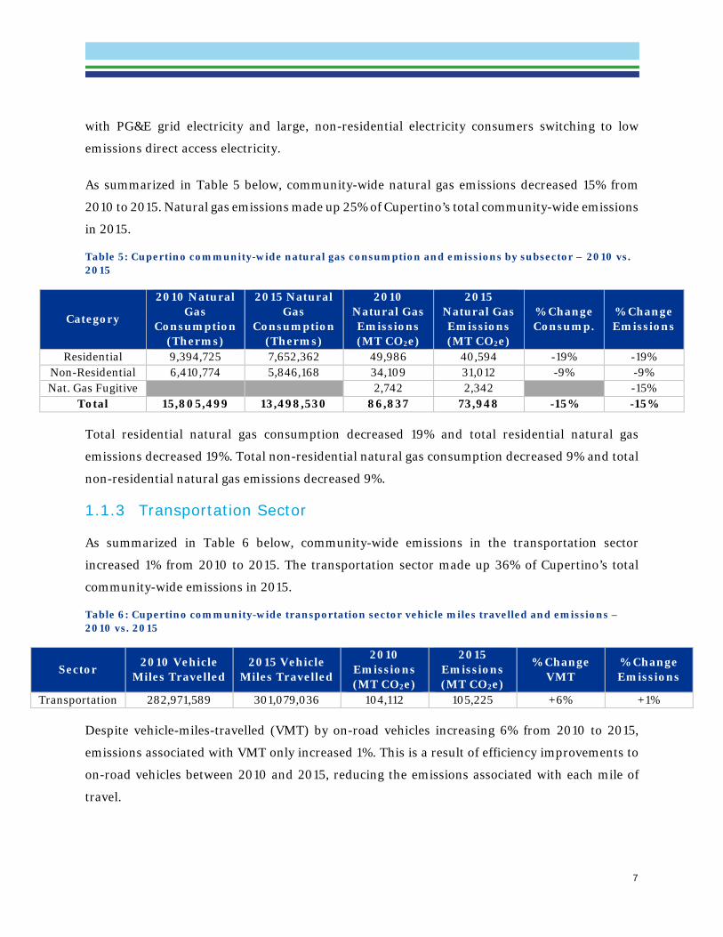
As summarized in Table 5 below, community-wide natural gas emissions decreased 15% from

2010 to 2015. Natural gas emissions made up 25% of Cupertino’s total community-wide emissions

in 2015.

Table 5: Cupertino community-wide natural gas consumption and emissions by subsector – 2010 vs. 2015

Total residential natural gas consumption decreased 19% and total residential natural gas

emissions decreased 19%. Total non-residential natural gas consumption decreased 9% and total

non-residential natural gas emissions decreased 9%.

1.1.3 Transportation Sector

As summarized in Table 6 below, community-wide emissions in the transportation sector

increased 1% from 2010 to 2015. The transportation sector made up 36% of Cupertino’s total

community-wide emissions in 2015.

Table 6: Cupertino community-wide transportation sector vehicle miles travelled and emissions – 2010 vs. 2015

Despite vehicle-miles-travelled (VMT) by on-road vehicles increasing 6% from 2010 to 2015,

emissions associated with VMT only increased 1%. This is a result of efficiency improvements to

on-road vehicles between 2010 and 2015, reducing the emissions associated with each mile of

travel.

Category

2010 Natural Gas

Consumption (Therms)

2015 Natural Gas

Consumption (Therms)

2010 Natural Gas Emissions (MT CO2e)

2015 Natural Gas Emissions (MT CO2e)

% Change Consump.

% Change Emissions

Residential 9,394,725 7,652,362 49,986 40,594 -19% -19% Non-Residential 6,410,774 5,846,168 34,109 31,012 -9% -9% Nat. Gas Fugitive 2,742 2,342 -15%

Total 15,805,499 13,498,530 86,837 73,948 -15% -15%

Sector 2010 Vehicle Miles Travelled

2015 Vehicle Miles Travelled



% Change VMT

% Change Emissions

Transportation 282,971,589 301,079,036 104,112 105,225 +6% +1%

8

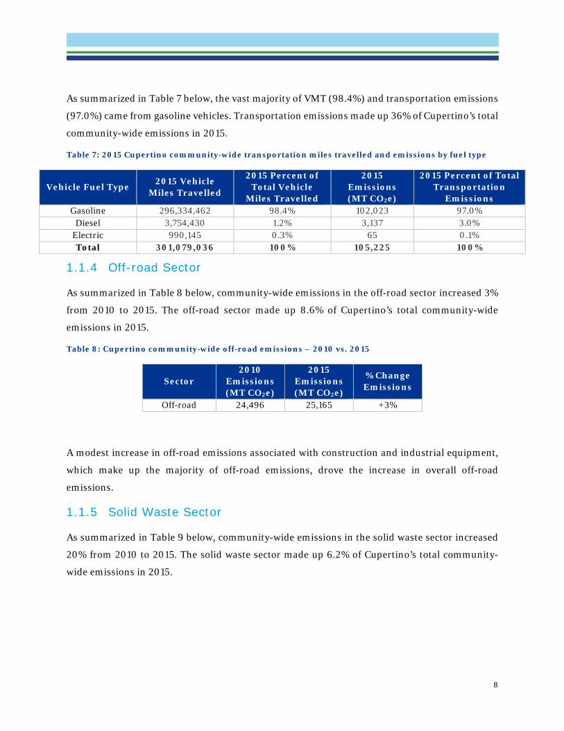
As summarized in Table 7 below, the vast majority of VMT (98.4%) and transportation emissions

(97.0%) came from gasoline vehicles. Transportation emissions made up 36% of Cupertino’s total

community-wide emissions in 2015.

Table 7: 2015 Cupertino community-wide transportation miles travelled and emissions by fuel type

1.1.4 Off-road Sector

As summarized in Table 8 below, community-wide emissions in the off-road sector increased 3%

from 2010 to 2015. The off-road sector made up 8.6% of Cupertino’s total community-wide

emissions in 2015.

Table 8: Cupertino community-wide off-road emissions – 2010 vs. 2015

A modest increase in off-road emissions associated with construction and industrial equipment,

which make up the majority of off-road emissions, drove the increase in overall off-road

emissions.

1.1.5 Solid Waste Sector

As summarized in Table 9 below, community-wide emissions in the solid waste sector increased

20% from 2010 to 2015. The solid waste sector made up 6.2% of Cupertino’s total community-

wide emissions in 2015.

Vehicle Fuel Type 2015 Vehicle Miles Travelled

2015 Percent of Total Vehicle

Miles Travelled


2015 Percent of Total Transportation

Emissions Gasoline 296,334,462 98.4% 102,023 97.0%

Diesel 3,754,430 1.2% 3,137 3.0% Electric 990,145 0.3% 65 0.1% Total 301,079,036 100% 105,225 100%

Sector 2010

Emissions (MT CO2e)


% Change Emissions

Off-road 24,496 25,165 +3%

9

Table 9: Cupertino community-wide solid waste landfilled and emissions – 2010 vs. 2015

Both the amount of solid waste sent to landfills and the emissions associated with landfilled waste

increased 20% from 2010 to 2015.

1.1.6 Wastewater Sector

As summarized in Table 10 below, community-wide emissions in the wastewater sector decreased

23% from 2010 to 2015. The wastewater sector made up 5.9% of Cupertino’s total community-

wide emissions in 2015.

Table 10: Cupertino community-wide wastewater emissions – 2010 vs. 2015

A 26% decrease in the 5-day biochemical oxygen demand (BOD5) – a measure used to evaluate

the effectiveness of wastewater treatment - at the San José-Santa Clara Regional Wastewater

Facility from 2010 to 2015 was the main driver behind the decrease in wastewater emissions.

Sector 2010 Waste Landfilled

(Tons)

2015 Waste Landfilled

(Tons)



% Change Waste

Landfilled

% Change Emissions

Solid Waste 30,685 36,817 15,185 18,219 +20% +20%

Sector

2010 5-day Biochemical

Oxygen Demand (kgBOD5/day)

2015 5-day Biochemical

Oxygen Demand (kgBOD5/day)



% Change Biochemical

Oxygen Demand

% Change Emissions

Wastewater 161,756 119,418 22,591 17,405 -26% -23%

10

1.2 2015 Municipal Operations Emissions Inventory 1.1.7 Summary of Municipal Operations Emissions Inventory Results

Our findings indicate that the City of Cupertino emitted municipal operations emissions of 1,440

MTCO2e in 2015 from the facilities, vehicle fleet, solid waste and water services sectors. This

represents a 22.8% decrease from 2010 municipal operations emissions of 1,865 MTCO2e.

Figure 3 and Table 11 provide a comparison of 2010 and 2015 municipal operations emissions and

trends by sector and subsector.

Figure 3: Cupertino municipal operations emissions by sector – 2010 vs. 2015

Facilities

Facilities

Vehicle Fleet

Vehicle Fleet

Solid Waste

Solid Waste

Water Services

Water Services

0

200

400

600

800

1,000

1,200

1,400

1,600

1,800

2,000

2010 2015

Annu

al E

mis

sion

s (M

T CO

2e)

11

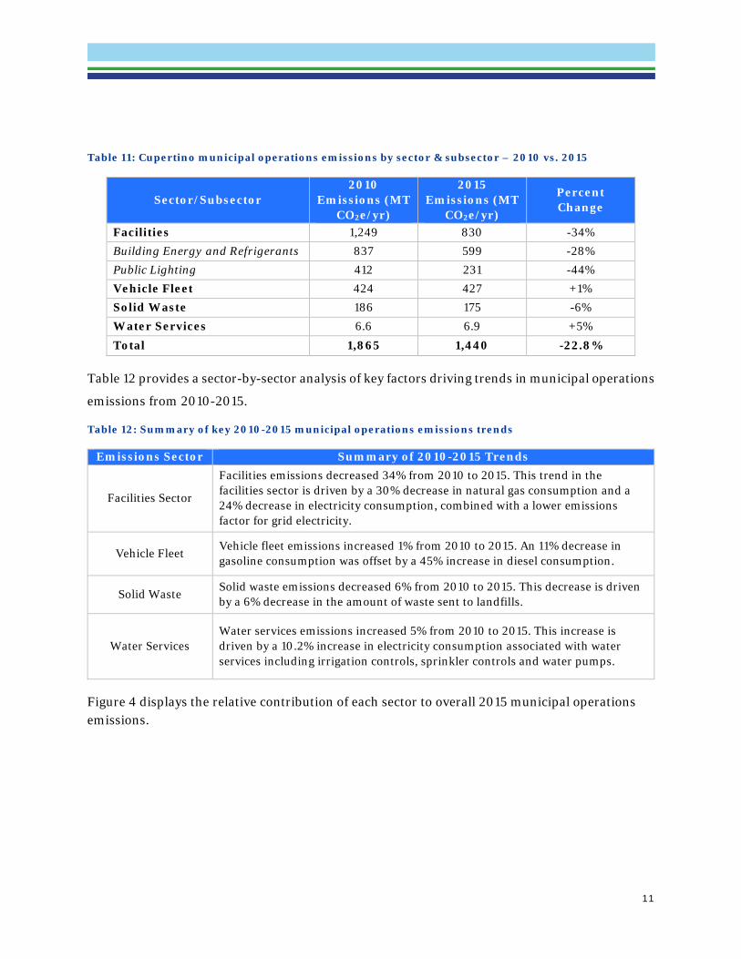
Table 11: Cupertino municipal operations emissions by sector & subsector – 2010 vs. 2015

Sector/Subsector 2010


2015 Emissions (MT

CO2e/yr)

Percent Change

Facilities 1,249 830 -34% Building Energy and Refrigerants 837 599 -28% Public Lighting 412 231 -44% Vehicle Fleet 424 427 +1% Solid Waste 186 175 -6%

Water Services 6.6 6.9 +5%

Total 1,865 1,440 -22.8%

Table 12 provides a sector-by-sector analysis of key factors driving trends in municipal operations

emissions from 2010-2015.

Table 12: Summary of key 2010-2015 municipal operations emissions trends

Emissions Sector Summary of 2010-2015 Trends

Facilities Sector

Facilities emissions decreased 34% from 2010 to 2015. This trend in the facilities sector is driven by a 30% decrease in natural gas consumption and a 24% decrease in electricity consumption, combined with a lower emissions factor for grid electricity.

Vehicle Fleet Vehicle fleet emissions increased 1% from 2010 to 2015. An 11% decrease in gasoline consumption was offset by a 45% increase in diesel consumption.

Solid Waste Solid waste emissions decreased 6% from 2010 to 2015. This decrease is driven by a 6% decrease in the amount of waste sent to landfills.

Water Services Water services emissions increased 5% from 2010 to 2015. This increase is driven by a 10.2% increase in electricity consumption associated with water services including irrigation controls, sprinkler controls and water pumps.

Figure 4 displays the relative contribution of each sector to overall 2015 municipal operations emissions.

12

Figure 4: 2015 municipal operations emissions by sector

Facilities (57.7%) and vehicle fleet (29.7%) continue to make up the vast majority of municipal

operations emissions in Cupertino. Solid waste (12.2%), and water services (0.5%) make up the

remaining municipal operations emissions.

Emissions associated with municipal employees commuting to work are scope 3 emissions from

the perspective of a municipal operations inventory because they are not directly controlled by

the city government. For this reason, employee commute emissions were not included in either

the 2010 or 2015 municipal operations inventories. However, employee commute surveys were

conducted for both 2010 and 2015. The results are presented below in Table 13.

Table 13: Cupertino municipal employee commute trends - 2010 vs. 2015

Description 2010 2015 Percent Change

All employees total driving commute emissions (MT CO2e) 463 443 -4.4% All employees total driving commute distance (miles/year) 1,244,509 1,272,985 +2.3%

Despite the total distance employees drove to work increasing 2.3% from 2010 to 2015, emissions

associated with employees driving to work decreased 4.4%. This is a result of employees driving

more fuel efficient vehicles to work in 2015.

57.7%29.7%

12.2%0.5%

Facilities

Vehicle Fleet

Solid Waste

Water Services

13

1.1.8 Facilities Sector

As summarized in Table 14 below, municipal operations emissions in the facilities sector

decreased 34% from 2010 to 2015. The facilities sector made up 58% of Cupertino’s total

municipal operations emissions in 2015.

Table 14: Cupertino municipal operations facilities sector consumption and emissions by subsector – 2010 vs. 2015

The overall decrease in facilities sector emissions was driven by a 44% decrease in total public

lighting emissions, a 30% decrease in facilities natural gas emissions and 28% decrease in

facilities electricity emissions. Emissions associated with electricity consumption declined at a

greater rate than electricity consumption itself due to a lower emissions factor for grid electricity.

1.1.9 Vehicle Fleet Sector

As summarized in Table 15 below, municipal operations emissions in the vehicle fleet sector

increased 1% from 2010 to 2015. The vehicle fleet sector made up 30% of Cupertino’s total


Category Consump.

Units 2010

Consump. 2015

Consump.



% Change Consump.

% Change Emissions

Facilities Electricity kWh 2,833,091 2,143,386 256 178 -24% -28%

Facilities Natural Gas

Therms 48,232 33,580 577 417 -30% -30%

Facilities Generators Gallons 52 116 0.5 1.4 +123% +197%

Facilities Refrigerants

3.6 2.8 -22%

Public Lighting Electricity

kWh 2,022,966 1,185,901 412 231 -41% -44%

Total 1,249 830 -34%

14

Table 15: Cupertino municipal operations vehicle fleet sector consumption and emissions by subsector – 2010 vs. 2015

The overall increase in facilities sector emissions was driven by a 4% increase in vehicle fleet fuel

emissions. An 11% decrease in vehicle fleet gasoline consumption was offset by a 45% increase in

diesel consumption.

1.1.10 Solid Waste Sector

As summarized in Table 16 below, municipal operations emissions in the solid waste sector

decreased 6% from 2010 to 2015. The solid waste sector made up 12% of Cupertino’s total


Table 16: Cupertino municipal operations solid waste sector consumption and emissions – 2010 vs. 2015

The 6% decrease in solid waste sector emissions is directly correlated with a 6% decrease in solid

waste landfilled.

1.1.11 Water Services Sector

As summarized in Table 17 below, municipal operations emissions in the water services sector

increased 5% from 2010 to 2015. The water services sector made up 0.5% of Cupertino’s total


Category Consump.

Units 2010

Consump. 2015

Consump.



% Change Consump.

% Change Emissions

Vehicle Fleet Fuel Gallons 41,025 41,721 379 393 +2% +4%

Vehicle Fleet Refrigerants

45 34 -23%

Total 424 427 +1%

Sector 2010 Waste Landfilled

(Tons)

2015 Waste Landfilled

(Tons)



% Change Waste

Landfilled

% Change Emissions

Solid Waste 376 355 186 175 -6% -6%

15

Table 17: Cupertino municipal operations water services sector consumption and emissions – 2010 vs. 2015

The 5% increase in water services sector emissions was driven by a 10% increase in water

services electricity consumption. Emissions associated with electricity consumption rose at a

lesser rate than electricity consumption itself due to a lower emissions factor for grid electricity.

Sector

2010 Electricity Consump.

(kWh)

2015 Electricity Consump.

(kWh)



% Change Electricity Consump.

% Change Emissions

Water Services

32,278 35,675 6.6 6.9 +10% +5%

16

1.3 2015 – 2050 Community-wide Emissions Forecast

Conducting an emissions forecast is an essential step in developing strategies to reduce emissions

and tracking progress towards established emissions reduction targets. Comparing projected

emissions according to growth scenarios for jobs, housing, and population against future potential

emissions reductions provides insight into whether a specific target level of reduction will be

achieved by a particular year based on policies currently in place.

As part of the community-wide inventory, emissions forecasts were created to estimate future

emissions out to 2020, 2035, and 2050 using the latest inventory (2015) as a starting point. These

forecast years were selected because they align with the following emissions reduction goals

Cupertino has established:

• 15% below 2010 emissions levels by 2020



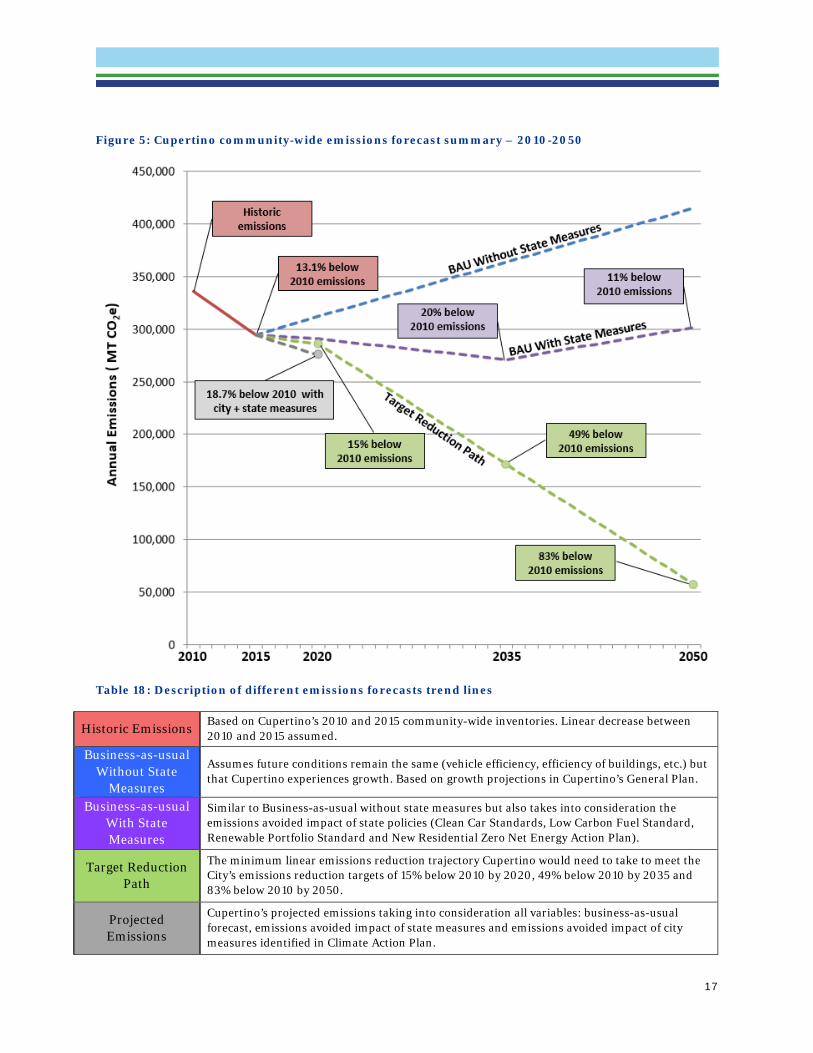
Figure 5 and Table 18 through Table 21Table 19 summarize historic emissions, the business-as-

usual emissions forecast, the City’s emissions reduction targets, emissions avoided from State

measures and the remaining emissions reductions that will be needed to achieve the emissions

reduction targets. Cupertino reduced its community-wide emissions 13.1% between 2010 and

2015 and, with implementation of measures identified in the CAP, is on pace to meet the City’s

emissions reduction target of 15% below 2010 emissions by 2020.

17

Figure 5: Cupertino community-wide emissions forecast summary – 2010-2050

Table 18: Description of different emissions forecasts trend lines

Historic Emissions Based on Cupertino’s 2010 and 2015 community-wide inventories. Linear decrease between 2010 and 2015 assumed.

Business-as-usual Without State

Measures

Assumes future conditions remain the same (vehicle efficiency, efficiency of buildings, etc.) but that Cupertino experiences growth. Based on growth projections in Cupertino’s General Plan.

Business-as-usual With State Measures

Similar to Business-as-usual without state measures but also takes into consideration the emissions avoided impact of state policies (Clean Car Standards, Low Carbon Fuel Standard, Renewable Portfolio Standard and New Residential Zero Net Energy Action Plan).

Target Reduction Path

The minimum linear emissions reduction trajectory Cupertino would need to take to meet the City’s emissions reduction targets of 15% below 2010 by 2020, 49% below 2010 by 2035 and 83% below 2010 by 2050.

Projected Emissions

Cupertino’s projected emissions taking into consideration all variables: business-as-usual forecast, emissions avoided impact of state measures and emissions avoided impact of city measures identified in Climate Action Plan.

18

Table 19: Cupertino community-wide historic emissions, emissions reduction target and emissions forecast – 2010-2020

Category Description Data Units

Historic Emissions and Current Progress

2010 Emissions: 338,673 MT CO2e

2015 Emissions: 294,281 MT CO2e

Percent Reduction Below 2010 by 2015: 13.1% Percent

2020 Emissions Reduction Target

Percent Reduction Below 2010 Target by 2020: 15% Percent

2020 Emissions Target: 287,872 MT CO2e 2020 Business-as-usual

Emissions and Emissions Reduction from State &

City Measures

2020 Business-as-usual Emissions: 312,152 MT CO2e

2020 Emissions Reduction from State Measures: -21,565 MT CO2e

2020 Emissions Reduction from City Measures: -15,400 MT CO2e

2020 Projected Emissions 2020 Projected Emissions with State + City Measures: 275,187 MT CO2e

Projected Percent Reduction Below 2010 by 2020: 18.7% Percent

Table 20: Cupertino community-wide emissions reduction target and emissions forecast – 2015-2035






City Measures



2035 Emissions Reduction from City Measures: MT CO2e



Table 21: Cupertino community-wide emissions reduction target and emissions forecast – 2015-2050






City Measures



2050 Emissions Reduction from City Measures: MT CO2e



Table 22 summarizes the estimated emissions avoided from State measures in 2020, 2035 and

2050.

19

Table 22 : Cupertino community-wide estimated emissions avoided from State measures in 2020, 2035, and 2050

State Measure Sector Impacted

2020 Emissions

Avoided (MT CO2e)

2035 Emissions

Avoided (MT CO2e)

2050 Emissions

Avoided (MT CO2e)

Clean Car Standards On-road transportation -15,150 -52,229 -60,900 Low Carbon Fuel Standard Off-road -667 -848 -1,028

Renewable Portfolio Standard All electricity -5,748 -33,888 -39,359 Zero Net Energy Action Plan Residential buildings 0 -5,640 -12,121

Total -21,565 -92,605 -113,408

20

1.4 Community-wide Inventory Methodology

The 2015 community-wide inventory follows GPC recommended methodologies and uses

Intergovernmental Panel on Climate Change (IPCC) Fifth Assessment Report (AR5) 100-year

without climate-carbon feedbacks global warming potentials (GWPs).4

1.1.12 Stationary Energy 1.1.12.1 Stationary Energy: Buildings

Activity Data

2015 community-wide natural gas and electricity consumption data was obtained through PG&E’s

Green Community website.5 PG&E electricity and natural gas consumption was broken out by the

residential, commercial and industrial sectors. However, with the exception of a few “district”

accounts, commercial and industrial energy consumption was combined into the commercial

sector. This is a result of CPUC energy data privacy rules that require PG&E to aggregate data

when customer privacy is at risk. The PG&E data also broke out total direct access electricity

consumption. Apple provided data on total direct access electricity consumption associated with

their Cupertino campus.6

Methodology

For the purposes of the GHG inventory, and to be in compliance with the GPC, all non-residential

energy consumption was placed into the “commercial & institutional buildings & manufacturing

industries & construction” subsector. All residential energy consumption was placed into the

“residential buildings” subsector. The emissions associated with the electricity consumed by

electric vehicles are accounted for in the transportation sector of the inventory, according to the

GPC guidance. However, electricity consumption associated with charging electric vehicles is

bundled into the electricity consumption data provided by PG&E. In order to avoid double

counting of electricity consumption and associated emissions in the stationary energy sector, the

estimated electricity consumption and emissions associated with electric vehicle charging were

subtracted from the stationary energy sector. Since an estimated 81% of electric vehicle charging

4 Greenhouse Gas Protocol, “Global Warming Potentials” www.ghgprotocol.org/sites/default/files/ghgp/Global-Warming-Potential-Values%20%28Feb%2016%202016%29_1.pdf 5 File downloaded from PG&E Green Community website titled “Cupertino_EXTNoNDA_PGE_CommunityGHG_2015”. 6 2015 Apple Cupertino direct access electricity consumption provided by Rick Freeman of Apple’s Global Energy Team via email on 5/30/17.

21

occurs at home7, 81% of total electricity consumption associated with electric vehicle charging was

subtracted from the residential buildings subsector and the remaining 19% was subtracted from

the commercial & institutional buildings & manufacturing industries & construction subsector.

See methodology description for the transportation sector for more details on how total electricity

consumption associated with electric vehicle charging was estimated.

Emission Factors

This inventory uses The Climate Registry (TCR) natural gas emission factor of 0.00530 MT

CO2/therm8 and a PG&E-specific electricity CO2 emission factor of 0.000197 MT CO2/kWh.9 To

account for fugitive natural gas emissions, the ICLEI ClearPath methodology was used. This

methodology assumes a 0.3% natural gas leakage rate, a natural gas energy density of 1028

btu/scf, a natural gas density of 0.8 kg/m3, 93.4% CH4 content in natural gas and 1% CO2 content

in natural gas. PG&E does not provide an electricity emission factor for methane (CH4) or nitrous

oxide (N2O), so 2014 Emissions & Generation Resource Integrated Database (eGRID) Western

Electricity Coordinating Council (WECC) emission factors of 0.000000015 MT CH4/kWh and

0.0000000018 MT N2O/kWh were used. 10 2015 emission factors were not available through

eGRID, so 2014 emission factors were used as a proxy.

Since the emission factor associated with the purchase of direct access electricity varies from

customer to customer, the average California statewide electricity emission factor was used as a

proxy. A direct access electricity emission factor was calculated by dividing the total California

electricity consumption in 2014 11 by the total California electricity-related GHG emissions in

2014. 12 The resulting direct access emission factors were 0.0002970315 MT CO2/kWh,

0.000000033 MT CH4/kWh and 0.0000000028 MT N2O/kWh. These direct access emission

7 PlugInsights, “81% of Electric Vehicle Charging is Done at Home”, December, 2013 http://insideevs.com/most-electric-vehicle-owners-charge-at-home-in-other-news-the-sky-is-blue/ 8 The Climate Registry, Table 12.1 U.S. Default Factors for Calculating CO2 Emissions from Fossil Fuel and Biomass Combustion www.theclimateregistry.org/wp-content/uploads/2016/03/2015-TCR-Default-EFs.pdf 9 2015 PG&E The Climate Registry Electric Power Sector Report 1.2 www.theclimateregistry.org/tools-resources/reporting-protocols/general-reporting-protocol/ 10 Emissions & Generation Resource Integrated Database (eGRID), 2014 www.epa.gov/energy/emissions-generation-resource-integrated-database-egrid 11 California Energy Commission Total System Electric Generation, “2014 Total System Electric Generation in Gigawatt Hours” www.energy.ca.gov/almanac/electricity_data/system_power/2014_total_system_power.html 12 California Air Resources Board, “Greenhouse Gas Emission Inventory - Query Tool for years 2000 to 2014 (9th Edition)” www.arb.ca.gov/app/ghg/2000_2014/ghg_sector.php

22

factors were applied to all direct access electricity consumption in Cupertino, with the exception

of direct access electricity purchase by Apple which is known to be 100% renewable.13

1.1.12.2 Stationary Energy: Off-Road

Activity Data

All off-road emissions were calculated using the ARB’s OFFROAD2007 Model.14

Methodology The OFFROAD2007 Model cannot be run on the city level. As a result, the model must be run at the County level and off-road emissions must be allocated to Cupertino based on the proportion of population or jobs in Santa Clara County (e.g. Santa Clara County’s industrial equipment emissions multiplied by the percent of total Santa Clara County jobs in Cupertino).

13 Apple Environmental Responsibility Report, “Scopes 1 & 2 Building Carbon Emissions (metric tons CO2e)” table, pages 30-31 https://images.apple.com/environment/pdf/Apple_Environmental_Responsibility_Report_2016.pdf 14 Air Resources Board, “Off-Road Emissions Inventory Program” www.arb.ca.gov/msei/offroad.htm

23

Table 23 below summarizes the type of off-road emissions in the OFFROAD2007 model output,

whether the emissions were included or excluded from the inventory, the GPC subsector

emissions were allocated to and the proxy (jobs or population) used to allocate Santa Clara County

emissions to Cupertino. Off-road emissions associated with airport ground support equipment,

agricultural equipment, pleasure craft, and oil drilling were excluded from the inventory because

those activities do not take place in Cupertino.

24

Table 23: Cupertino community-wide off-road emissions – included and excluded

Cupertino’s 2015 population15 and Santa Clara County’s 2015 population16 are from the US Census.

2015 employment data for Santa Clara County and Cupertino was not available at the time this

inventory was published. As a result, Cupertino’s 2011 employment17 and Santa Clara County’s

2010 employment18 were used as a proxy to estimate the percent of total employment in Santa

Clara County occurring in Cupertino.

Emission Factors:

Emissions in terms of N2O exhaust, CH4 exhaust and CO2 exhaust are a direct output of the

OFFROAD2007 model. As a result, emission factors were not required to calculate emissions

associated with the off-road sector.

1.1.13 Transportation

Activity Data:

The origin-destination methodology was used to estimate total VMT in Cupertino. As part of the

General Plan, an origin-destination VMT model for 2013 was developed by Hexagon for

15 United States Census QuickFacts, City of Cupertino www.census.gov/quickfacts/table/PST045216/0617610 16 United States Census QuickFacts, County of Santa Clara www.census.gov/quickfacts/table/HCN010212/06085 17 California, State of, 2011. Employment Development Department. Monthly Labor Force Data for Cities and Census Designated Places, September 2011-Preliminary. https://s3.amazonaws.com/Apple-Campus2-DEIR/Apple_Campus_2_Project_EIR_Public_Review_5c-PopHousing.pdf 18 Bay Area Census, County of Santa Clara. www.bayareacensus.ca.gov/counties/SantaClaraCounty.htm

OFFROAD 2007 Type of Emissions Included or Excluded?

GPC Subsector Percent of County

Emissions Allocated to Cupertino By:

Construction and Mining Equipment Included Commercial & Institutional Jobs Industrial Equipment Included Commercial & Institutional Jobs

Light Commercial Equipment Included Commercial & Institutional Jobs Railyard Operations Included Commercial & Institutional Jobs

Transport Refrigeration Units Included Commercial & Institutional Population Entertainment Equipment Included Residential Buildings Population

Lawn and Garden Equipment Included Residential Buildings Population Recreational Equipment Included Residential Buildings Population

Airport Ground Support Equipment Excluded Agricultural Equipment Excluded

Pleasure Craft Excluded Oil Drilling Excluded

25

Cupertino. This model was used to estimate 2010 VMT for the 2010 inventory. However, since

the same model used to calculate 2010 and 2013 VMT was not available, this inventory relied on

publically available Cupertino-specific origin-destination VMT data available through the

Metropolitan Transportation Commission (MTC) to estimate a 2010-2015 VMT annual growth

rate in Cupertino.19 This annual growth rate was applied to the Hexagon 2013 VMT to estimate

the 2015 VMT.

Methodology

Similar to the 2010 inventory, total VMT was separated into two categories – passenger cars and

trucks. All VMT associated with trucks was assumed to be non-electric. In order to estimate the

percent of passenger car VMT from electric vehicles, data on 2015 Santa Clara County VMT

travelled by fuel type from the ARB’s EMFAC Web Database was used.20 This process assumes

that the percent of total VMT attributable to electric vehicles in Santa Clara County is equal to the

percent of total Cupertino VMT attributable to electric vehicles.

Emission Factors:

The EMFAC Web Database was also used to translate VMT travelled by specific vehicles types into

GHG emissions through the utilization of EMFAC’s vehicle-specific emission factors. However,

EMFAC does not include assumptions regarding the emission factors/efficiency of electric

vehicles. In order to translate electric vehicle VMT to electricity consumption, the average

efficiency (kWh/mile) of the three best-selling electric vehicles in 2015 was used.21 See section

1.1.12.1 for an explanation of the electricity emission factor used in this inventory.

For non-electric passenger cars, EMFAC fuel efficiencies were used to translate VMT into CO2

emissions. EMFAC does not include CH4 and N2O emission factors, so EPA emission factors by

vehicle type for CH4 and N2O were used.22 EMFAC groups fuel efficiencies by vehicle type.23

Consistent with the 2010 inventory, all passenger car VMT was assumed to be travelled by LDA,

LDT1 and LDT2 vehicle types. The same process was used to translate truck VMT into emissions.

19 MTC Cupertino origin-destination VMT data for calendar years 2010 and 2015 provided by Harold Brazil of MTC ([email protected]). 20 EMFAC Web Database EMFAC2014 (v1.0.7). For the model run the calendar year selected was "2015", the season selected was "annual" and the vehicle classification selected was "EMFAC2011 Categories". 21 Average efficiency of 2015 Nissan Leaf, 2015 Chevrolet Volt and 2015 Toyota Prius plug-in from Department of Energy’s www.fueleconomy.gov www.fueleconomy.gov/feg/findacar.shtml 22 Environmental Protection Agency “Emission Factors for Greenhouse Gas Inventories” www.epa.gov/sites/production/files/2015-07/documents/emission-factors_2014.pdf 23 See following website for a complete list of EMFAC vehicle categories: www.arb.ca.gov/msei/vehicle-categories.xlsx

26

Consistent with the 2010 inventory, all truck VMT was assumed to be travelled by LHD1, LHD2,

PTO, SBUS, T6 Ag, T6 CAIRP heavy, T6 CAIRP small, T6 instate construction heavy, T6 instate

construction small, T6 instate heavy, T6 instate small, T6 OOS heavy, T6 OOS small, T6 Public,

T6 utility, T7 Ag, T7 CAIRP, T7 CAIRP construction, T7 NNOOS, T7 NOOS, T7 other port, T7

POAK, T7 Public, T7 Single, T7 single construction, T7 SWCV, T7 tractor, T7 tractor construction,

T7 utility, T6TS, and T7IS vehicle types.

1.1.14 Waste 1.1.14.1 Waste: Solid Waste Disposal

Activity Data:

This inventory used data on the amount of Cupertino waste sent to landfills in 2015 from

CalRecycle’s Disposal Reporting System (DRS): Jurisdiction Disposal and Alternative Daily Cover

(ADC) Tons by Facility web portal. 24 Data on waste composition is from CalRecycle's 2014

Disposal-Facility-Based Characterization of Solid Waste in California.25

Methodology & Emission Factors:

The GPC methane commitment method for waste emissions was used. Tonnages of disposed

waste sent to landfills and waste composition were input into GPC Equations 8.1, 8.3 and 8.4 to

calculate CH4 emissions associated with disposed waste. For Equation 8.1, the default carbon

content values were used. For equation 8.3, the default fraction of methane recovered in landfill

was used and an oxidation factor of 0.1 was selected because the landfills Cupertino sends waste

to are managed. For equation 8.4, default values for the fraction of degradable organic carbon

degraded and the fraction of methane in landfill gas were used. A methane correction factor of

1.00 was used because the landfills Cupertino sends waste to are actively managed.

24 Disposal Reporting System (DRS) : Jurisdiction Disposal and Alternative Daily Cover (ADC) Tons by Facility www.calrecycle.ca.gov/LGCentral/Reports/DRS/Destination/JurDspFa.aspx 25 See Table ES-3 "Composition of California's Overall Disposed Waste Stream by Material Type". www.calrecycle.ca.gov/publications/Documents/1546/20151546.pdf

27

1.1.14.2 Waste: Wastewater

Activity Data:

This inventory used data on population served by the San José-Santa Clara Regional Wastewater

Facility from the San José Environment website.26 Data on Cupertino’s 2015 population form the

US Census was used. 27 Data on the 5-day biochemical oxygen demand 28 and average total

nitrogen per day29 of the San José-Santa Clara Regional Wastewater Facility from the San José-

Santa Clara Regional Wastewater Facility 2015 Annual Self Monitoring Report was used.


The GPC, the U.S. Community Protocol for Accounting and Reporting of Greenhouse Gas

Emissions (Community Protocol) and the LGO Protocol methodologies for calculating wastewater

treatment emissions are all derived from the 2006 IPCC Guidelines for National Greenhouse Gas

Inventories, Volume 5, chapter 6: Wastewater Treatment and Discharge. 30 Available data for

wastewater treatment plants varies considerably from plant to plant, and as a result inventories

use the combination of available equations from these three protocols that match the data inputs

available for the particular plant that serves their community. Cupertino is served by the San José-

Santa Clara Regional Wastewater Facility, which is located in San José. Based on available data,

San José’s 2014 community inventory used a combination of LGOP Equation 10.2, Community

Protocol Equation WW.2 (alt), Community Protocol Equation WW.6 and Community Protocol

Equation WW.12 to calculate CH4 emissions and N2O emissions associated with the plant.31 For

this reason, and because these methodologies are derived from the 2006 IPCC Guidelines for

National Greenhouse Gas Inventories and in compliance with the GPC, these same methodologies

were used in this inventory. This approach not only ensures consistency with the GPC, but also

ensures regional consistency with San José’s inventory.

26 San Jose Environment, “San José-Santa Clara Regional Wastewater Facility” www.sanjoseca.gov/Index.aspx?NID=1663 27 United States Census QuickFacts, City of Cupertino. www.census.gov/quickfacts/table/PST045216/0617610 28 San José-Santa Clara Regional Wastewater Facility 2015 Annual Self Monitoring Report, “BOD Loadings 2015 (kg/d)” table, page 8 www.sanjoseca.gov/ArchiveCenter/ViewFile/Item/2797 29 San José-Santa Clara Regional Wastewater Facility 2015 Annual Self Monitoring Report, page 19 www.sanjoseca.gov/ArchiveCenter/ViewFile/Item/2797 30 See www.ipcc-nggip.iges.or.jp/public/2006gl/pdf/5_Volume5/V5_6_Ch6_Wastewater.pdf 31 San José’s 2014 community inventory, pages A-10 and A-11 www.sanjoseca.gov/DocumentCenter/View/55505

28

1.5 Municipal Operations Inventory Methodology

The 2015 municipal operations inventory follows LGOP recommended methodologies and uses

Intergovernmental Panel on Climate Change (IPCC) Fifth Assessment Report (AR5) 100-year

without climate-carbon feedbacks global warming potentials (GWPs).32

1.1.15 Facilities 1.1.15.1 Facilities: Building Energy

Activity Data:

2015 municipal operations natural gas and electricity consumption data was obtained through

PG&E’s Green Community website.33 Data on fuel consumption by municipal generators was

provided by the City.

Methodology:

Accounts associated with buildings and facilities were pulled from this data and grouped into the

building energy subsector. Most accounts matched one-to-one to accounts labeled as buildings

and facilities accounts in the 2010 inventory. New accounts were identified as belonging to

buildings based on account descriptions provided by PG&E.

Emission Factors:

See section 1.1.12.1 for an explanation of the electricity and natural gas emission factors used in

this inventory. Gasoline, diesel and propane emission factors used to calculate generator

emissions are from the U.S. Energy Information Administration.34

1.1.15.2 Facilities: Building Refrigerants

Activity Data:

Data on stationary refrigeration equipment name, type of equipment, the full charge capacity of

the equipment, and the type of refrigerant consumed by the equipment was provided by the City.

32 Greenhouse Gas Protocol, “Global Warming Potentials” www.ghgprotocol.org/sites/default/files/ghgp/Global-Warming-Potential-Values%20%28Feb%2016%202016%29_1.pdf 33 See www.pge.com/en_US/business/save-energy-money/contractors-and-programs/community-partnerships/community-partners.page 34 U.S. Energy Information Association, “Carbon Dioxide Coefficients” www.eia.gov/environment/emissions/co2_vol_mass.php

29

Table 6.4 from the LGOP was used to look up the operating emission factor of each piece of

equipment.


Emissions were calculated using the above inputs and Equation 6.35 from the LGOP. Global

warming potential of various refrigerants are from table E.2 of the LGOP.

1.1.15.3 Facilities: Public Lighting

Activity Data:

2015 municipal operations electricity consumption data was obtained through PG&E’s Green

Community website.35

Methodology:

Accounts associated with public lighting were pulled from this data and grouped into the public

lighting subsector. Most accounts matched one-to-one to accounts labeled as public lighting

accounts in the 2010 inventory. New accounts were identified as belonging to public lighting

based on account descriptions provided by PG&E. The public lighting subsector was further

broken down into other outdoor lighting, park lighting, streetlights and traffic signals/controls.

Emission Factors:

See section 1.1.12.1 for an explanation of the electricity emission factor used in this inventory.

1.1.16 Water Services

Activity Data:

2015 municipal operations electricity consumption data was obtained through PG&E’s Green

Community website.36

Methodology:

Accounts associated with water services were pulled from this data and grouped into the water

services subsector. Most accounts matched one-to-one to accounts labeled as water services

accounts in the 2010 inventory. New accounts were identified as belonging to water services based

on account descriptions provided by PG&E.

35 See www.pge.com/en_US/business/save-energy-money/contractors-and-programs/community-partnerships/community-partners.page 36 See www.pge.com/en_US/business/save-energy-money/contractors-and-programs/community-partnerships/community-partners.page

30

Emission Factors:

See section 1.1.12.1 for an explanation of the electricity emission factor used in this inventory.

1.1.17 Vehicle Fleet 1.1.17.1 Vehicle Fuel

Activity Data:

Monthly gasoline and diesel consumption for all vehicles in the City’s fleet was provided by the

City.


Gasoline and diesel CO2 emission factors used to calculate fleet fuel emissions are from the U.S.

Energy Information Administration.37 Gasoline and diesel CH4 and N2O emission factors used to

calculate fleet fuel emissions are from the Environmental Protection Agency’s 2008 National

Emissions Inventory (NEI) Data.38

1.1.17.2 Vehicle Refrigerants

Activity Data:

Data on vehicle make and model, type of mobile equipment, and the type of refrigerant consumed

by the equipment was provided by the City. Table 7.2 from the LGOP was used to look up the full

charge capacity and operating emission factor of each piece of equipment.


Emissions were calculated using the above inputs and Equation 7.13 from the LGOP. Global

warming potential of various refrigerants are from table E.2 of the LGOP.

1.1.18 Solid Waste

Activity Data:

37 U.S. Energy Information Association, “Carbon Dioxide Coefficients” www.eia.gov/environment/emissions/co2_vol_mass.php 38 Environmental Protection Agency’s 2008 National Emissions Inventory (NEI) Data www.epa.gov/air-emissions-inventories/2008-national-emissions-inventory-nei-data

31

Data on waste collection sites, number of dumpsters at each site, volume of dumpsters at each

site, and frequency of dumpster pick-ups was provided by the City. As with the 2010 inventory,

all dumpsters were estimated to be 75% full. In order to convert volume of waste landfilled to

weight of waste landfilled, a CalRecycle waste volume to weight conversion factor specific to

“government operations” waste was used.39


The methodology for calculating waste emissions matches that used in the community-wide

inventory. See section 1.1.14.1 of this document for a full description.

39 CalRecycle Solid Waste Characterization Home www2.calrecycle.ca.gov/WasteCharacterization/

32

1.6 2015-2050 Community-wide Emissions Forecast Methodology

1.1.19 Business-as-usual Forecast Without State Measures

The first step in the emissions forecasting process is to create a business-as-usual forecast that

does not factor in state measures. This scenario assumes that conditions remain the same (vehicle

efficiency, efficiency of buildings, etc.) but that Cupertino experiences growth. Business-as-usual

emissions growth rates in sector were based off projected growth rates in population, employment

or VMT. See Table 24 below

Table 24: Cupertino business-as-usual forecast emissions growth rate proxies by sector

Population and job projections for Cupertino for 2015, 2020, 2035 and 2050 from the CAP were

used.40 VMT projections for Cupertino for 2015 and 2035 from MTC were used.41 Since VMT

projections for 2020 and 2050 from MTC were not available, it was assumed that the linear

growth rate in VMT between 2015 and 2035 would hold constant in order to estimate 2020 and

2050 VMT.

1.1.20 Business-as-usual Forecast With State Measures

The second step in the emissions forecasting process is to adjust the business-as-usual forecast to

account for the emissions reduction impact of State measures. Four key state measures were

considered – California’s Clean Car Standards, the Low Carbon Fuel Standard (LCFS), the

Renewable Portfolio Standard (RPS), and the New Residential Zero Net Energy Action Plan.

Clean Car Standards

Emissions avoided from California’s Clean Car Standards were estimated using the projected

future fuel efficiencies for years 2020, 2035 and 2050 from ARB’s EMFAC Web Database. The

percent increase in fuel efficiency from the base year (2015) to the forecast year (e.g. 2020) was

calculated in order to estimate emissions avoided from the Clean Car Standards in the forecast

40 City of Cupertino Climate Action Plan, Appendix B - GHG Inventory and Reductions Methodology page B-9, Table B-2 41 MTC Cupertino origin-destination VMT data for calendar years 2015 and 2035 provided by Harold Brazil of MTC ([email protected]).

Sector Growth Rate Used as Proxy for Business-as-usual Emissions Growth in Sector

Residential Population Commercial/Industrial Employment

Transportation VMT Waste & Wastewater Average of Population & Employment

33

year. Emissions reduction associated with Clean Car Standards were applied to forecasted on-

road transportation emissions.

Low Carbon Fuel Standard (LCFS)

Emissions avoided from the LCFS were estimated using ARB’s projection of a 7.2% reduction in

transportation emissions below 2005 levels by 2020 resulting from the policy.42 This translates

to a 2.4% reduction in transportation emissions below 2015 levels by 2020. Emissions

reductions associated with the LCFS were only applied to forecasted off-road emissions.

Emissions reductions were not applied to forecasted on-road transportation emissions to

avoided double counting of emissions avoided from the Clean Car Standards.

Renewable Portfolio Standard (RPS)

Emissions avoided form the RPS were estimated using data from PG&E on the percent of 2015

electricity procured from renewable sources (30%) and the State’s RPS targets for 2020 (33%)

and 2030 (50%).43 The percent increase in renewables between 2015 and each forecast year, as a

result of the RPS, was translated to a percent decrease in electricity emissions using an analysis

by E3 focused on this topic.44 The RPS was assumed to plateau at 50% renewables in 2030 since

there is currently no RPS target in place beyond 2030. Emissions reductions associated with the

RPS were applied to all forecasted electricity emissions.

New Residential Zero Net Energy Action Plan

Emissions avoided form the New Residential Zero Net Energy Action Plan were estimated using

projections on the number of new households in Cupertino from 2010 to 2040 from the CAP.45

This data was used to estimate the number of new residential construction projects that would

be impacted between 2020 (when the policy goes into effect) and 2050. It was estimated that

1.12% of the residential building stock would be replaced per year from 2020-2050 and the new

homes built to a zero net energy standard would reduce energy consumption 55% compared to a

42 California Air Resources Board, Proposed Regulation to Implement the Low Carbon Fuel Standard, 2009 www.arb.ca.gov/fuels/lcfs/030409lcfs_isor_vol1.pdf 43 PG&E’s 2015 Power Mix www.pge.com/pge_global/common/pdfs/your-account/your-bill/understand-your-bill/bill-inserts/2016/11.16_PowerContent.pdf 44 E3, “Investigating a Higher Renewables Portfolio Standard in California”, 2014 www.ethree.com/wp-content/uploads/2017/01/E3_Final_RPS_Report_2014_01_06_with_appendices.pdf 45 City of Cupertino Climate Action Plan, Appendix B - GHG Inventory and Reductions Methodology page B-9, Table B-2

34

typical existing home in 2015.46 Emissions reductions associated with zero net energy residential

construction were applied to forecasted residential building emissions.

46 Zero net energy residential building codes only apply to “regulated loads”, which make up approximately 55% of total residential energy use.

35

1.7 Adjustments to 2010 Baseline Inventories

One of the inherent challenges with GHG inventories is that inventory protocols and

methodologies are constantly evolving. Additionally, GWPs of CH4 and N2O are also changing

with each new Assessment Report released by the IPCC. These two variables can make

comparisons between past and current inventories challenging.

1.1.21 Adjustments to the 2010 Community-wide Inventory

Cupertino’s original 2010 community-wide inventory was completed following the Community

Protocol, while this 2015 community-wide inventory was completed following the GPC. At the

time the 2010 community-wide inventory was completed, the Community Protocol was the most

commonly used protocol for cities completing GHG inventories. However, in recent years, the

GPC has become the standard protocol, in part because it is required for those cities who have

committed to the Global Covenant.

GWP is a relative measure of how much heat a greenhouse gas traps in the atmosphere. It

compares the amount of heat trapped by a certain mass of the gas in question to the amount of

heat trapped by a similar mass of CO2. At the time the 2010 community-wide inventory was

completed, GWP values from the IPCC Fourth Assessment Report (AR4) were the current

accepted standard. However, in 2014, AR5 was released. Between AR4 and AR5 the GWP of CH4

increased from 25 to 28 and the GWP of N2O decreased from 298 to 265. In order to make “apples-

to-apples” comparisons between the 2010 and 2015 community-wide inventories and accurately

track Cupertino’s emissions reduction progress, it was necessary to revise the 2010 emissions to

match the methodology and GWPs used in the 2015 inventory. Table 25 below compares the

original 2010 and revised 2010 community-wide inventories. Rows highlighted in red indicate an

adjustment to the original 2010 community-wide inventory.

36

Table 25: Cupertino community-wide emissions – 2010 original vs. 2010 revised

Sector/Subsector 2010 Original


2010 Revised Emissions

(MT CO2e/yr) Percent Change

Energy 169,547 172,289 +2% Electricity Subtotal 85,451 85,451 0%

Residential 25,427 25,427 0% Commercial 60,025 60,025 0%

Natural Gas Subtotal 84,095 86,837 +3% Residential 49,986 49,986 0% Commercial 34,109 34,109 0% Fugitive Nat. Gas 0 2,742 N/A

Transportation 104,112 104,112 0% Off-Road Sources 22,390 24,496 +9% Solid Waste 5,403 15,185 +181% Wastewater 4,640 22,591 +387% Potable Water 1,197

Total 307,288 338.673 10.2%

Sector-by-sector adjustments to 2010 community-wide inventory

The energy, off-road sources, solid waste, wastewater and potable water sectors were adjusted in

the revised 2010 community-wide inventory.

• Energy: The original 2010 inventory was based on the Community Protocol which does

not require the inclusion of fugitive natural gas emissions. Since the GPC calls for the

inclusion of fugitive natural gas emissions, the 2010 community-wide inventory was

revised to include these emissions.

• Off-road Sources: Both inventories used ARB’s OFFROAD2007 model to estimate

emission from off-road sources. However, the original inventory excluded off-road

emissions from transport refrigeration units, entertainment equipment, recreational

equipment and railyard operations. The GPC calls for these emissions to be included, and,

as a result, the 2010 community-wide inventory was revised to include these emissions.

• Solid Waste: There are two generally acceptable methods for estimating waste emissions

- the methane commitment method and the first order of decay (FOD) method. The

methane commitment method allocates emissions based on the quantity of waste disposed

during the inventory year, while the FOD method allocates emissions based on the

quantity of waste disposed during the inventory year as well as existing waste in landfills.

37

The original 2010 inventory used the FOD method to estimate waste emissions. However,

after discussion with City staff, it was decided that the 2015 inventory should use the

methane commitment method because emissions associated with the methane

commitment method are more closely linked to current waste practices, rather than waste

historically sent to landfills. As a result, the 2010 community-wide inventory was revised

to estimate waste emissions using the methane commitment method. Additionally, 2010

waste emissions were adjusted to account for the AR5 GWP of CH4, opposed to the AR4

GWP originally used.

• Wastewater: Both inventories used the same general approach of determining total San

José-Santa Clara Regional Wastewater Facility emissions and then allocating a

proportional amount of total plant emissions to Cupertino based on service population.

However, the original 2010 community-wide inventory used total SJ-SC RWF emissions

from The Plant Master Plan (2013)47. This methodology was not compliant with the GPC

because it did not account for methane emissions from lagoons, a substantial portion of

SJ-SC RWF’s emissions. As a result, the 2010 community-wide inventory was revised to

estimate wastewater emissions using the recommended GPC methodology. Additionally,

2010 waste emissions were adjusted to account for the AR5 GWPs of CH4 and N2O,

opposed to the AR4 GWPs originally used.

• Potable Water: The Community Protocol called for cities to include emissions

associated with water conveyance electricity consumption occurring outside the city

boundary. However, since this electricity consumption occurs outside of city boundaries,

the GPC does not instruct cities to report these emissions. As a result, emissions associated

with water conveyance were not included in the 2015 community-wide inventory or the

revised 2010 community-wide inventory.

47 See www.sanjoseca.gov/DocumentCenter/View/38425

38

1.1.22 Adjustments to the 2010 Municipal Operations Inventory

Both the 2010 and 2015 municipal operations inventories followed the LGO protocol. However,

assumptions related to the calculation of waste emissions in the original 2010 municipal

operations inventory relied on a “USA default” waste composition variable and the complete

methodology for estimating emissions was not fully documented. The 2015 municipal operations

inventory used waste composition data from CalRecycle and followed recommended GPC

methodologies for calculating waste emissions using the methane commitment method. 48

Additionally, the original 2010 municipal operations inventory used the AR2 GWP for CH4, while

the 2015 inventory used the AR5 GWP for CH4. In order to make apples-to-apples comparisons

between the 2010 and 2015 municipal operations inventories and track Cupertino’s municipal

emissions reduction progress, the original 2010 waste emissions were revised to reflect more

accurate waste composition data and an updated CH4 GWP. Table 1 below compares the original

2010 and revised 2010 municipal operations inventories.

Table 26: Municipal operations emissions – 2010 original vs. 2010 revised

Emissions Sector 2010 Original


2010 Revised Emissions

(MT CO2e/yr) Percent Change

Facilities 1,249 1,249 0% Building Energy and Refrigerants 837 837 0%

Public Lighting 412 412 0% Vehicle Fleet 424 424 0% Solid Waste 95.3 186 95% Water Services 6.6 6.6 0% Total 1,775 1,865 5.1%

48 2014 Disposal-Facility-Based Characterization of Solid Waste in California, Table ES-3 "Composition of California's Overall Disposed Waste Stream by Material Type"

39

About DNV GL

Driven by our purpose of safeguarding life, property and the environment, DNV GL enables organizations to advance the safety and sustainability of their business. We provide classification and technical assurance along with software and independent expert advisory services to the maritime, oil and gas, and energy industries. We also provide certification services to customers across a wide range of industries. Operating in more than 100 countries, our 16,000 professionals are dedicated to helping our customers make the world safer, smarter and greener.

Date post:	18-Mar-2022
Category:	Documents
Upload:	others
View:	2 times
Download:	0 times