City, University of London Institutional Repository

Citation: Tomas-Rodriguez, M. & Banks, S. P. (2013). An iterative approach to eigenvalue assignment for nonlinear systems. International Journal of Control, 86(5), pp. 883-892. doi: 10.1080/00207179.2013.765037

This is the unspecified version of the paper.

This version of the publication may differ from the final published version.

Permanent repository link: http://openaccess.city.ac.uk/2430/

Link to published version: http://dx.doi.org/10.1080/00207179.2013.765037

Copyright and reuse: City Research Online aims to make research outputs of City, University of London available to a wider audience. Copyright and Moral Rights remain with the author(s) and/or copyright holders. URLs from City Research Online may be freely distributed and linked to.

City Research Online: http://openaccess.city.ac.uk/ publications@city.ac.uk

City Research Online

1

An Iterative Approach to Eigenvalue Assignmentfor Nonlinear Systems.

M.Tomas-Rodrigueza∗ and S.P.Banksb

aThe City University, School of Engineering and Mathematical Sciences, London, UK.bAutomatic Control and Systems Engineering Department, TheSheffield University,

UK.

Abstract

In this paper, the authors present a method for controlling anonlinear system by using the ideas ofeigenvalues assignment. A time-varying approach to nonlinear exponential stability via eigenvalue placementis studied based on an iteration technique that approaches anonlinear system by a sequence of linear time-varying equations. The convergent behaviour of this methodis shown and applied to a practical nonlinearexample in order to illustrate these ideas.

Index Terms

Nonlinear systems, Eigenstructure Assignment, Pole placement, Iteration.

I. I NTRODUCTION

The aim of this paper is to design a feedback controller so that the original nonlinear system isstabilized according to some requirements. The pole placement idea for linear time invariant systemsis extended to a general pole placement technique applicable to linear time-varying systems and withthe aid of an iteration technique presented in [Tomas-Rodriguez et al.(2003)], ultimately to nonlinearsystems in a general form. Several authors approached the pole placement idea for general nonlinearsystems in the past; Most of these techniques have in common the idea of linearizing the nonlinearsystem about a countable set of equilibrium points and finding a single controller that will stabilize eachmember of the finite countable set (see [Chow(1990)] for example). On the other hand, within the areaof nonlinear systems, and having its origins in the geometric control theory, exact feedback linerizationwith pole placement is achieved by following a two-step design method as in [Isidori(1989)] and[Sontag(1998)]. There have been as well attempts to obtain both feedback linearization and poleplacement objectives in just one step as in [Kazantzis et al.(2000)].

Pole placement for linear time invariant systems has been the object of diverse studies: Some of themwere based on Ackerman′s formula [Ackermanet al.(1972)], others approached the problem by usinga periodic output feedback ([Greschak et al.(1990)], [Aeyels et al.(1991)]) for second order systemsor even arbitrary order as in [Aeyels et al.(1992)].The original pole placement method for linear time invariant SISO systems was first extended tolinear time-varying systems by [Silverman(1966)] using a canonical representation of the originalsystem. Since then, it had been several contributions by different authors to develop pole placementtechniques for linear time-varying systems (i.e. [Silverman(1966)], [Tuel(1967)], [Luenberger(1967)],[Kailath(1980)], [Varga(1981)], [Miminis(1982)], [Petkov et al.(1985)], [Kautsky et al.(1985)], [Choi(1995)],[Choi(1996)], [Choi(1998)] or [Bhattacharyya et al.(1982)]). More recently, Valaseket.al. initiated

∗Corresponding author. Email: Maria.Tomas-Rodriguez.1@city.ac.uk

2

a series of publications related to the eigenvalue placement problem based on the extension ofAckerman′s formula to linear time-varyingSISO and later to linear time invariant and linear time-varying MIMO systems in which the eigenvalue placement was based on the equivalence of theclosed-loop original system via a Lyapunov transformationto a linear time invariant system withpoles at prescribed locations ([Valasek et al.(1995)], [Valasek et al.(1995b)], [Valasek et al.(1999)]).It should be pointed out that an important limitation of the pole placement algorithm is the lack ofguaranteed tracking performance. This topic is treated in more general output feedback approaches.A typical remedy for this involves the incorporation of theInternal Model Principleinto the controllaw design ([Francis et al.(1976)] and [Bengtsson(1977)]) or the inclusion of integrators into the loop.This issue will not be addressed in this paper, since pole placement design is the main interest here.

The contents of this article are based on the classical pole placement method for linear time invariantsystems and the iteration technique presented in [Tomas-Rodriguez et al.(2003)], [Tomas-Rodriguez et al.(2010)].The objective is to develop a pole placement method for nonlinear systems of the form:

x = f(x) = A(x)x(t) + B(x)u(t), x(0) = x0.

Replacing the nonlinear system above by a sequence of linear time-varying systems, a sequence offeedback laws of the formu(i)(t) = K(i)(t)x(i)(t) can be generated: for each of them, the closed-looppoles for theith linear time-varying system at each time of the time intervalare allocated to somedesired locationσ = (λ1d, · · ·λnd) where eachλi can be time-varying or constant. This iterationtechnique is presented in Section II.It is well-known that linear time-varying systems can be unstable despite having left half-plane poles;that is, for linear time-varying systems, poles do not have the same stability meaning as in the timeinvariant case, so the allocation of the pole in the left handside plane does not guarantee the stabilityof the closed-loop system. In order to overcome this probleman approach to stability using Duhamel’sprinciple is presented in Section III where conditions based on differentiability of the eigenvector′smatrix are derived.From the convergence properties of the sequence of linear time-varying solutions, [Tomas-Rodriguez et al.(2003)],by choosing theK(i)(t) feedback gain corresponding to theith iteration and applying the limiting valueto the closed-loop nonlinear system, the pole placement andstability objectives are achieved for a widevariety of nonlinear cases. This generalization to nonlinear systems is given in Section IV, followed bya numerical example in Section V. Section VI contains the conclusions and further research guidelines.

II. I TERATION TECHNIQUE FORNONLINEAR SYSTEMS

This section recalls a recently introduced technique for nonlinear dynamical systems in which theoriginal nonlinear equation is replaced by a sequence of linear time-varying equations convergingin the space of continuous functions to the solution of the nonlinear system under a mild Lipschitzcondition [Tomas-Rodriguez et al.(2003)]. This method has also been used in optimal control theory[Tomas-Rodriguez et al.(2005)], in the design of nonlinear observers [Navarro-Hernandez et al.(2003)]or control of a super-tanker [Tayfun Cimen et al.(2004)] to cite a few. Any nonlinear system of theform

x = f(x) = A(x)x, x(0) = x0 ∈ Rn. (1)

whereA(x) is locally Lipschitz can be approximated by a sequence of linear time-varying equations:

x(1) = A[x(0)]x(1), x(1)(0) = x(0)...

x(i) = A[x(i−1)]x(i), x(i)(0) = x(0)

(2)

for i ≥ 1. The solutions of this sequence of linear time-varying equations converge to the solution

3

of the nonlinear system given in (1). The convergence of these sequence is stated in the followingtheorem:Suppose that the nonlinear equation (1) has a unique solution on the interval[0, τ ] denoted byx(t)

and assume thatA : Rn → Rn is locally Lipschitz. Then the sequence of functions definedin (2)converges uniformly on[0, τ ] to the solutionx(t).

The convergence of Theorem II is proved in [Tomas-Rodriguez et al.(2003)] where global conver-gence is extended to time intervalst ∈ [0,∞]. The application of this technique gives an accuraterepresentation of the nonlinear solution after a few iterations. Nonlinear systems satisfying the localLipschitz requirement can be now approached by common linear techniques. This is a very mildassumption, and is already assumed for the uniqueness of solution in Theorem II.

III. E IGENVALUE ASSIGNMENT FORL INEAR TIME-VARYING SYSTEMS

A. General approach to pole placement

In this section the pole-placement method for linear time invariant cases will be extended to lineartime-varying systems of the form:

x(t) = A(t)x(t) +B(t)u(t), x(0) = x0 (3)

wherex(t) ∈ Rn is the vector of the measurable states,u(t) ∈ Rm is the control signal andA(t),B(t) are time-varying matrices of appropriate dimensions.Given a set of desired stable eigenvalues,σ =

(λ1d · · ·λnd

)and a time interval[0, t], the aim is to

place the closed-loop eigenvalues of (3) at those desired points ∀t ∈ (0, t) by using a convenient statefeedback controlu(t) = −K(t)x(t) where the feedback gainK(t) is a time dependent function.

Given that the pair[A(t), B(t)

]is controllable for allt ∈ [0, t], the eigenvalue placement theorem is

applied to (3):det∣∣∣λ · I − [A(t)− B(t)K(t)]

∣∣∣ = (λ− λ1d) · · · (λ− λnd) (4)

and by solving (4), a time-varying feedback gainK(t) can be determined so that the closed-loop formof the system (3) will now be of the form

x(t) = [A(t)−B(t)K(t)]x(t) = A(t)x(t) (5)

with stable eigenvalues on the left-half plane at(λ1 · · ·λn

)=(λ1d · · ·λnd

). In order to guarantee

stability of the system (3), further issues should be taken into account as for linear time-varyingsystems, the existence of negative closed-loop poles is nota sufficient condition for stability.In the following sections, conditions for exponential stability of linear time-varying systems withnegative eigenvalues will be derived and these results willbe extended for the nonlinear case.

B. Sufficient stability conditions for linear time-varyingsystems

Having in mind that the matrixA(t) already has negative eigenvalues by (4), some other conditionsfor stability of the closed-loop system (5) should be satisfied, these conditions can be summarizedin the following theorem: Given the open loop linear time-varying systemx = A(t)x(t) + B(t)u(t),x0 = x(0), whose closed-loop matrixA(t) = A(t)−B(t)K(t) has designed left hand-plane eigenvaluesσ = (λ1d, . . . , λnd) via the feedback signalu(t) = −K(t)x(t) and assuming the following conditionsto be satisfied:

I/ λ1d is the eigenvalue ofA(t) with the greatest real part,II/ The matrix of eigenvectorsP (t) is differentiable,

III/ ||P−1(t)P (t)|| < β,

4

then forβ < Re(λ1d) the closed-loop system

x = [A(t)− B(t)K(t)]x(t) = A(t)x(t)

is exponentially stable.Proof: The system (5) can be solved over any time interval[0, t], by dividing the interval intoNsubintervals of lengthh, such thath = t/N → 0 whenN → ∞, using Duhamel′s principle,

x(t) = limh→0

(eA[Nh]h · eA[(N−1)h]h . . . eA[h]h · I · x0

)(6)

Applying the similarity transformeA(t) = P (t)eΛ(t)P−1(t) to (6) yields:

x(t) =(PNe

Λ[Nh]hP−1N

)·(PN−1e

Λ[(N−1)h]hP−1N−1

)· · ·

(P1e

Λ[h]hP−11

)· I · x0 (7)

whereΛ(t) ∈ Cnxn is a diagonal matrix of desired eigenvalues andP (t) ∈ Cnxn is the time-varyingmatrix of the corresponding eigenvectors.PN is P (t) at time t = Nh.Λ(t) is considered to be time-varying to generalize the results of Theorem III-B. In this particulararticle it is considered to be constant as the desired eigenvalues were taken to be constant.The second assumption was thatP (t) was differentiable, therefore its Taylor expansion will beof theform:

P (t+ h) = P (t) + hdP (t)

dt+

h2

2!

d2P (t)

dt+ · · · (8)

Neglecting high order terms and noting thatdP (t)dt

= P (t):

P (t+ h) = P (t) + hP (t) (9)

By inverting both sides of equation (9), post-multiplying byP (t) and, using the approximation(1 + a)−1 ≈ 1− a+ · · · , we obtain:

P (t+ h)−1P (t) ≈[I − P (t)−1hP (t)

](10)

and,P (t+ h)−1 · P (t) ≈ I + ǫ(h) (11)

whereǫ = o(h), so thatǫ → 0 ash → 0.

Thus, (7) can be written as:

x(t) = PN · eΛ[Nh]h · (I + ǫ) · eΛ[(N−1)h]h · (I + ǫ) · · · eΛ[h]hP1 · I · x0 (12)

Taking norms of the above expression, a bound on the norm ofx(t) can be estimated by,

||x(t)|| ≤ ||PN || · ||(1 + ǫ)||N · ||P1|| · ||e(Λt)|| · ||x0|| (13)

and taking into account that||eΛt|| ≤ eRe(−λmax)t

whereλmax is the eigenvalue of the matrixΛ with largest real part, then forλmax = λ1d

||x(t)|| ≤ ||PN || · ||(I + ǫ)||N · ||P1|| · e−λ1dt · ||x0||. (14)

Now, it was shown in (11) thatǫ(h) = −hP−1(t)P (t), so

||I + ǫ|| = ||I − hP−1P (t)|| ≤ 1 + h||P−1(t)P (t)||

5

By AssumptionIII in Theorem III-B, ||P−1(t)P (t)|| is bounded byβ, and ||I + ǫ(h)|| ≤ 1 + hβ.

Therefore,||x(t)|| ≤ ||PN || · (1 + hβ)N · ||P1|| · e

−λ1dt · ||x0||

and

(1 + hβ)N =

(1 +

βt

N

)N

→ eβt

so||x(t)|| ≤ ||PN || · e

(β−λ1d)t · ||P1|| · ||x0||.

Analyzing the expression above for exponential stability,PN , P1, and x0 are constant values, soet(β−λ1d) → 0 is required:

e(β−λ1d)t → 0, (β − λ1d) < 0 → β < |λ1d|. (15)

That is, for exponential stability, the closed-loop eigenvaluesλd should be chosen so that the greatestof them λ1d satisfies (15) which represents a compromise between the upper bound of the rate ofchange ofP (t) andλ1d.

C. A Necessary condition for the differentiability ofP (t)

In the previous section it was shown how the exponential stability properties of the closed-loopsystem relied upon the satisfaction of conditionsI-III in Theorem III-B. These conditions weresufficient conditions for stability. In this section a necessary condition for stability will be derived.This condition is given in terms of a differential equation which places restrictions onΛ(t), K(t) andP (t). The necessary condition for stability is stated as follows: The differentiability of the matrix ofeigenvectorsP (t) (andA(t), B(t), K(t) andΛ(t)) imply that the following equation is satisfied:[A(t)− B(t)K(t)−B(t)K(t)

]= P (t)

[Λ(t)− Λ(t)P−1(t)P (t) + P−1(t)P (t)Λ(t)

]P−1(t), (16)

whereΛ(t) is the diagonal matrix of eigenvalues ofA(t) andK(t) is the feedback gain designed forstable closed loop poles. Proof: Consider twonearby time pointst and t + h, and evaluatethe similarity transforms at those points keeping in mind that the matrixΛ(t) is a diagonal matrixcontaining the eigenvalues of the matrix

[A(t)− B(t)K(t)

]= A(t):

P−1(t) [A(t)−B(t)K(t)]P (t) = Λ(t) (17)

P−1(t+ h) [A(t+ h)− B(t+ h)K(t+ h)]P (t+ h) = Λ(t+ h) (18)

as in (8) and the assumed differentiability ofA(t), B(t) andK(t). Then,

A(t+ h) = A(t) + hA(t) + · · ·

B(t+ h) = B(t) + hB(t) + · · ·

K(t+ h) = K(t) + hK(t) + · · ·

and by the differentiability ofP (t) and (10);

P−1(t+ h) = P−1(t)− hP−1(t)P (t)P−1(t)

it follows that (18) can be written as

Λ(t+ h) =[P−1(t)− hP−1(t)P (t)P−1(t)

]·[A(t) + hA(t)−

(B(t) + hB(t)

)·(K(t) + hK(t)

)]·

·[P (t) + hP (t)

]= Λ(t) + hΛ(t).

6

Expanding and rejecting high order terms yields:

Λ(t)+hΛ(t) =[P−1(t)−hP−1(t)P (t)P−1(t)

]·[A(t)+hA(t)−B(t)K(t)−hB(t)K(t)−hBK(t)

]·[P (t)+hP (t)

]

this is,

Λ(t) + hΛ(t) = P−1(t)[A(t)−B(t)K(t)

]P (t) + P−1(t)h

[A(t)−B(t)K(t)

]P (t)

+P−1(t)h[A(t)− B(t)K(t)−B(t)K(t)

]P (t)− hP−1(t)P (t)P−1(t)

[A(t)−B(t)K(t)

]P (t).

(19)Taking into account thatP−1(t)

[A(t)−B(t)K(t)

]P (t) = Λ(t) andP−1(t)h

[A(t)−B(t)K(t)

]P (t) =

hΛ(t)P−1(t)P (t), now equation (19) can be written as:

Λ(t)+hΛ(t) = Λ(t)+hΛ(t)P−1(t)P (t)−hP−1(t)P (t)Λ(t)+hP−1(t)[A(t)−B(t)K(t)−B(t)K(t)

]P (t).

Dividing by h on both sides a differential equation inΛ(t) is obtained:

Λ(t) = P−1(t)[A(t)− B(t)K(t)−B(t)K(t)

]P (t) + Λ(t)P−1(t)P (t)− P−1(t)P (t)Λ(t) (20)

or

P−1(t)[A(t)− B(t)K(t)− B(t)K(t)

]P (t) = Λ(t)− Λ(t)P−1(t)P (t) + P−1(t)P (t)Λ(t). (21)

Multiplying on the left byP−1(t) and on the right byP (t), then:[A(t)− B(t)K(t)−B(t)K(t)

]= P (t)

[Λ(t)− Λ(t)P−1(t)P (t) + P−1(t)P (t)Λ(t)

]P−1(t). (22)

To summarize: IfP (t), A(t), B(t), K(t) andΛ(t) are differentiable (which we require in order toprove Theorem III-B, then (22) must be satisfied. If it is not, then Theorem III-B does not strictlyapply. However, as shown in the following example,P (t) may not be differentiable at a discrete setof points of the time intervalt ∈ [0, t] and the result will still hold.

D. Example

Given the following linear time-varying open loop system:

x(t) =

ecos(t) log

[1

1+t2

]

t2 t

x(t) +

(1

1

)u(t),

with initial conditionsx(0) = [0.5, 0.5]T . The aim is to set the closed-loop poles atσ = (−8,−6).When the pole placement method is applied, it can be seen in Figure 1.a that despite the poles beingsuccessfully allocated at the designed location, the shapeof the response shows a jump along thetime interval and so does the designed controlu(t) = −K(t)x(t), (Figure 1.b). Plotting the profileof ǫ(h), it can be seen it reflects the two discontinuities at timest = 1.1 secs andt = 2.68 secs,where the condition for differentiability ofP (t) fails (Figure 2.a). In Figure 2.b an estimate of thedifferentiability of P (t) is shown, it is represented by the quantityP (t+h)−P (t)

hcalculated at each step

h of the time interval. As expected it shows two discontinuities along the interval[0, tf ], the first onehappening att = 1.1 sec and the second one att = 2.68 sec. On the other hand, if now the locationof the poles is shifted to be i.e.σ = (−12,−10), Figures 3.a and 3.b show the components of theresponse and the control law for this choice of left hand sidepoles.This time it can be seen how the discontinuities in the stableresponses and the control after the poleplacement are smoother than in the previous case. The plot ofepsilonǫ(h) in Figure 4 clearly showstwo discontinuities too, verifying the existence of the relation betweenP (t), Λ(t), A(t), B(t) andK(t) as indicated in (22). As the desired poles have changed, so did Λ(t) and consequentlyK(t) andP (t) and its differentiability.

7

TIME (sec)

TIME (sec)

x(t

)1

x(t

)2

(a)

TIME (sec)

Co

ntr

ol

u(t

)

(b)

Fig. 1: (a) Components of the responsex1(t), x2(t). The shape of the response shows a jump att = 1.1seconds. (b) Control signalu(t) = −Kx(t) for the desired set of chosen polesσ = (−8,−6). Theshape ofu(t) shows a jump att = 1.1 seconds

IV. GENERALIZATION TO NONLINEAR SYSTEMS

In this section an approach to the problem of pole placement when the system under considerationis nonlinear is presented. A nonlinear system of the form:

x = A(x)x(t) + B(x)u(t), x(0) = x0 (23)

whereA(x) ∈ Rnxn, B(x) ∈ Rmxn, u(t) is the control signal andx(0) = x0 is the vector containingthe given initial conditions. (23) can be written as a sequence of linear time-varying systems:

x(1) = A(x0)x(1)(t) + B(x0)u

(1)(t), x(1)(0) = x0

... (24)

x(i) = A(x(i−1)(t))x(i)(t) + B(x(i−1)(t))u(i)(t), x(i)(0) = x0

Applying the methodology presented in Section III, for somegiven choice of closed-loop poles, i.e.σ = (λ1d, · · ·λnd), a sequence of feedback control laws of the formu(i)(t) = −K(i)(t)x(i)(t) isobtained at each iterationi, eachK(i) is the feedback gain obtained to ensure stability on each of theiterates closed-loop forms:

x(1) = [A(x0(t))− B(x0(t))K(1)(t)]x(1)(t), x(1)(0) = x0

... (25)

x(i) = [A(x(i−1)(t))− B(x(i−1)(t))K(i)(t)]x(i)(t), x(i)(0) = x0

Now, the eigenvalue placement theorem can be applied to eachof these systems (25) being the set ofdesired polesσ = (λ1d, · · ·λnd) chosen to be the same for each iteration:

det[λ · I − A(x0) + B(x0)K(1)(t)] = (λ− λ1d) · · · (λ− λnd)

... (26)

8

TIME (sec)

Ep

silo

n

(a)

TIME (sec)

Dif

fere

nti

ab

ilit

y o

f P

(t)

(b)

Fig. 2: (a) ǫ(h) shows discontinuities at timest = 1.1 seconds andt = 2.68 seconds where thecondition for differentiability ofP (t) fails. (b) Differentiability of P (t) is lost at the same timeswhereǫ(h) is discontinuous.

det[λ · I − A(x(i−1)(t)) + B(x(i−1)(t))K(i)(t)] = (λ− λ1d) · · · (λ− λnd)

Therefore, each of these linear time-varying closed loop systems (25) will be exponentially stableprovided the conditions from Section III-C are satisfied.After a finite number of iterations, the solutionx(i)(t) converges to the nonlinear solutionx(t). Then,the last iterated feedback gainK(i)(t) that stabilises the”ith” system, can be applied to the originalnonlinear system in order to satisfy the stability requirements for this nonlinear closed-loop:

x = [A(x(t))−B(x(t))K(i)(t)]x(t), x(0) = x0

provided that the desired eigenvaluesσ = (λ1, · · ·λn) are chosen to be far on the left-half plane asstated in Section III-C.

The exponential stability of the nonlinear system achievedas indicated here can be summarized asfollows: Given a nonlinear system of the form (23) where the matricesA(x) andB(x) are Lipschitzand the pair(A,B) is controllable∀x(t), ∀t ∈ [0, T ], there exists a feedback controlu(t) given by:

limi→∞u(i)(t) = limi→∞K(i)(t)x(t) → u(t)

whereK(i)(t) is Lipschitz, such that the solutionx(t) of the nonlinear system is exponentially stable in[0, T ]. Proof: We need to assume thatK(i)(t) satisfies the Lipschitz condition at each iteration,(differentiability is a necessary condition for exponential stability of the linear time-varying systemson the sequence) and also thatA(x) and B(x) are Lipschitz, then, the iteration technique can beapplied. By applying the pole placement algorithm, an algebraic equation is set and solved at eachiteration in order to obtain the elements of the corresponding feedback gain matrixK(i)(t);

λn + Γ(i)n−1λ

n−1 + Γ(i)n−2λ

n−2 + · · ·+ Γ(i)1 λ1 + λ0 = (λ− λ1)(λ− λ2) · · · (λ− λn) (27)

The coefficientsΓ(i)j are a linear combination of the linear elements ofK(i)(t) =

[k(i)1 (t), . . . , k(i)

n (t)].

9

TIME (sec)

TIME (sec)

x(t

)1

x(t

)2

(a)

TIME (sec)

Co

ntr

ol

u(t

)

(b)

Fig. 3: (a) Components of the responsex1(t), x2(t). The shape of the response shows a smoother jumpthan in the previous case. (b) Controlu(t) = −Kx(t) when the poles of the close loop are shifted toσ = (−12,−10).

TIME (sec)

Ep

silo

n

Fig. 4: ǫ(h) shows two discontinuities. This verifies the existence of the relation betweenP (t), Λ(t),A(t), B(t) andK(t) as indicated in (22)

In order to solve this, identification of parameters needs tobe performed at this stage, simply byequating the coefficients on both sides of equation (27):

Γ(i)n−1 = α

(i)n−1 + β

(i)n−1 · k

(i)n−1(t) = φn−1(λ1, · · · , λn)

Γ(i)n−2 = α

(i)n−2 + β

(i)n−2 · k

(i)n−2(t) = φn−2(λ1, · · · , λn)...

Γ(i)1 = α

(i)1 + β

(i)1 · k

(i)1 (t) = φ1(λ1, · · · , λn)

(28)

Therefore, the elements ofK(i)(t) of the feedback gain can be obtained by solving each of theequations in (28):

k(i)n−1(t) =

φ(i)n−1(λ1,··· ,λn)−α

(i)n−1

β(i)n−1

, · · · · · · , k(i)1 (t) =

φ(i)1 (λ1,··· ,λn)−α

(i)1

β(i)1

(29)

10

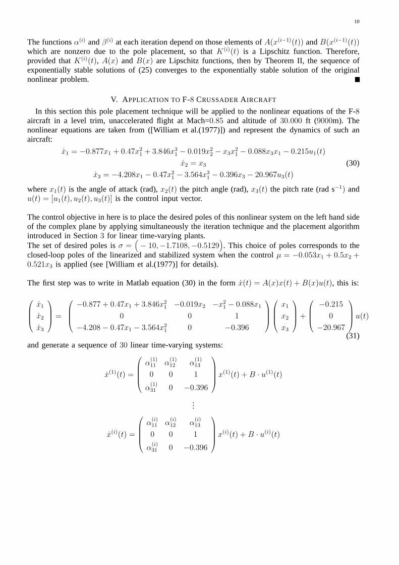
The functionsα(i) andβ(i) at each iteration depend on those elements ofA(x(i−1)(t)) andB(x(i−1)(t))which are nonzero due to the pole placement, so thatK(i)(t) is a Lipschitz function. Therefore,provided thatK(i)(t), A(x) andB(x) are Lipschitz functions, then by Theorem II, the sequence ofexponentially stable solutions of (25) converges to the exponentially stable solution of the originalnonlinear problem.

V. A PPLICATION TO F-8 CRUSSADERA IRCRAFT

In this section this pole placement technique will be applied to the nonlinear equations of the F-8aircraft in a level trim, unaccelerated flight at Mach=0.85 and altitude of30.000 ft (9000m). Thenonlinear equations are taken from ([William et al.(1977)]) and represent the dynamics of such anaircraft:

x1 = −0.877x1 + 0.47x21 + 3.846x3

1 − 0.019x22 − x3x

21 − 0.088x3x1 − 0.215u1(t)

x2 = x3

x3 = −4.208x1 − 0.47x21 − 3.564x3

1 − 0.396x3 − 20.967u3(t)

(30)

wherex1(t) is the angle of attack (rad),x2(t) the pitch angle (rad),x3(t) the pitch rate (rad s−1) andu(t) = [u1(t), u2(t), u3(t)] is the control input vector.

The control objective in here is to place the desired poles ofthis nonlinear system on the left hand sideof the complex plane by applying simultaneously the iteration technique and the placement algorithmintroduced in Section3 for linear time-varying plants.The set of desired poles isσ =

(− 10,−1.7108,−0.5129

). This choice of poles corresponds to the

closed-loop poles of the linearized and stabilized system when the controlµ = −0.053x1 + 0.5x2 +0.521x3 is applied (see [William et al.(1977)] for details).

The first step was to write in Matlab equation (30) in the formx(t) = A(x)x(t) + B(x)u(t), this is:

x1

x2

x3

=

−0.877 + 0.47x1 + 3.846x21 −0.019x2 −x2

1 − 0.088x1

0 0 1

−4.208− 0.47x1 − 3.564x21 0 −0.396

x1

x2

x3

+

−0.215

0

−20.967

u(t)

(31)and generate a sequence of30 linear time-varying systems:

x(1)(t) =

α(1)11 α

(1)12 α

(1)13

0 0 1

α(1)31 0 −0.396

x(1)(t) + B · u(1)(t)

...

x(i)(t) =

α(i)11 α

(i)12 α

(i)13

0 0 1

α(i)31 0 −0.396

x(i)(t) + B · u(i)(t)

11

TIME (sec)

TIME (sec)

TIME (sec)

An

gle

of

att

ack

Pit

ch a

ngle

Pit

ch r

ate

(a)

TIME (sec)

CO

NT

RO

L

(b)

Fig. 5: (a) Closed Loop response. Statesx1(t), x2(t) andx3(t). (b) Control lawu(t).

with

α(1)11 = −0.877 + 0.47x1(0) + 3.846x2

1(0), α(1)12 = −0.019x2,

α(1)13 = −x2

1(0)− 0.088x1(0), α(1)31 = −4.208− 0.47x1(0)− 3.564x2

1(0),

α(i)11 = −0.877 + 0.47x

(i−1)1 + 3.846

(x(i−1)1

)2

, α(i)12 = −0.019x

(i−1)2 ,

α(i)13 = −

(x(i−1)1

)2

− 0.088x(i−1)1 , α

(i)31 = −4.208− 0.47x

(i−1)1 − 3.564

(x(i−1)1

)2

,

B = [−0.215, 0,−20.967]T

where the initial conditions arex(0) = [x1(0), x2(0), x3(0)] = [0.5253, 0, 0]T . At each iteration”i” afeedback lawu(i)(t) = −K(i)(t)x(i)(t) is designed following the specifications: this is, the closed-looppoles at each iteration should be allocated atλd =

(− 10,−1.7108,−0.5129

),

x(i)(t) = A(x(i−1)(t))x(i)(t)−B(x(i−1)(t))K(i)(t)x(i)(t) = A(x(i−1)(t))x(i)(t)

whereA(x(i−1)(t)) is the closed-loop matrix for theith iteration. Using Ackerman′s formula:

det[λ · I − A(x(i−1)(t))

]=(λ− λ1

)(λ− λ2

)(λ− λ3

), (32)

in this way, a feedback matrixK(i−1)(t) at each iteration is obtained. The simulations for each iterationwere carried outtf = 15 sec with a time step ofh = 0.01. After 30 iterations, the sequence of lineartime-varying systems converges to the nonlinear system; taking the30th feedback control and applyingthis to the nonlinear system,

x(t) = A(x)x(t)−B(x)K(30)(t)x(t)

it can be seen how the states of the nonlinear system convergeto zero, Figure 5.a. The control lawapplied to the nonlinear system is shown in Figure 5.b, it presents an isolated discontinuity in thedifferentiability of the matrix of eigenvaluesP (t); this does not affect the states as shown in Figure5.a.It is shown how the pitch angle variable,x2(t) and the pitch ratex3(t) go beyondπ radians, which

12

is a non realistic scenario. In spite of this, both states reach exponential stability within the workingtime interval, this is the main purpose of this numerical example, to demonstrate convergence of thepresented method and exponential stability achievement. The scenario in spite of being representedby a highly nonlinear equation is not intended to be a realistic one, in fact, the full set of equations ofmotion of a fighter aircraft is not3-dimensional like in this case. Issues such as robustness, adequacyof the methodology, minimization of overshoot maximum value...etc, have not being dealt with asthey are not under study in this work. All these issues are currently investigated by the authors andthe findings will be presented in a future contribution.

VI. CONCLUSIONS

In this article a pole-placement algorithm for nonlinear systems has been presented. The method isbased on the application of an iteration technique that replaces the nonlinear system by a sequenceof linear time-varying systems.Once this sequence of linear time-varying systems has been obtained, a standard pole-placementprocedure is applied for each of the linear time-varying systems by dividing the interval inN stepsof length h and applying Duhamel′s principle. It has been shown how this method alone does notguarantee stability for linear time-varying systems and therefore additional requirements for stabilitywere developed in Section 3:If the matricesA(t), B(t), P (t) andK(t) are differentiable, then, writing equation (22) in the form:

Λ = P−1(t)(A(t)− B(t)K(t)−B(t)K(t)

)P (t) + Λ(t)P−1(t)P (t)− P−1(t)P (t)Λ(t) (33)

gives a coupled equation relatingP (t), K(t) andΛ(t) which states that these are not independent.Hence, in general, it may not be possible (in some cases) to chooseΛ constant. Thus, equation (33)is an important condition for the exponential stability of the already pole placed linear time-varyingsystem.The restriction it places onP (t), K(t) andΛ(t) at the moment are the object of further research.These results were extended to nonlinear systems by the convergence of the iteration technique, thusthe feedback gain designed for the last of the linear time-varying iterated systems is applied to thenonlinear system and achieving in this way exponential stability. Due to the accurate approach of theiteration technique to the original nonlinear plant, this pole placement method results in a more robustmethod than those relying on the linearization of the original system, at least the uncertainties of theunmodelled original dynamics do not exist in this case.Some numerical examples were presented showing how the technique works and showing that, evenin the case where differentiability ofP (t) is not satisfied at every point of the time interval[0, t], thenonlinear system can be stabilized using this technique.

REFERENCES

[Ackermanet al.(1972)] Ackerman, J. (1972),Abtastregelung, Berlin/New York, Springer-Verlag, ISBN 0387057072.

[Aeyels et al.(1991)] Aeyels, D. and Willems, J.L. (1991), “Pole assignment for linear time-invariant second-order systems by periodicstatic output feedback.”IMA J. of Mathematical Control and Information, 8, 267-274.

[Aeyels et al.(1992)] Aeyels, D. and Willems, J.L., (1992), “Pole assignment for linear time-invariant systems by periodic memorylessoutput feedback.”Automatica, 28, 1159-1168.

[Bengtsson(1977)] Bengtsson, G. (1977), “Output regulations andinternal models- a frequency domain approach.”Automatica, 13,333-345.

[Bhattacharyya et al.(1982)] Bhattacharyya, S.P. and De Souza, E. (1982), “Pole assignment via Sylvester′s equation.”Systems andControl letters, 1, 261-263.

13

[Choi(1995)] Choi, J. W., Lee, L. G., Kim, Y. and Kang, T. (1995),“Design of an effective controller via disturbance accomodatingleft eigenstructure assingment.”AIAA Journal of Guidance, Control and Dynamics, 18, 347-354.

[Choi(1996)] Choi, J. W., Lee, L. G., Suzuki, H. and Suzuki, T. (1996), “Comments on Matrix Method of Eigenstructure Assignment:The multi-input Case with application.”AIAA Journal of Guidance, Control and Dynamics, 19, 983.

[Choi(1998)] Choi, J.W. (1998), “Left eigenstructure assignmentvia the Sylvester equation.”KSME International Journal, 12,1034-1040.

[Chow(1990)] Chow, J.H. (1990), “A Pole-Placement Design Approach for Systems with Multiple Operating Conditions.”IEEETransactions on Automatic Control, 35(3), 278-288.

[Francis et al.(1976)] Francis, B. A. and Wonham, W. M. (1976), “The internal model principle of control theory.”Automatica, 12,457-465.

[Greschak et al.(1990)] Greschak, J. P. and Verghese, G.C. (1990), “Periodically varying compensation of time-invariant systems.”Syst. Control Lett., 2, 88-93.

[Isidori(1989)] Isidori, A. (1989), Springer-Verlag, London., “Nonlinear Control Systems: An introduction.”

[Kailath(1980)] Kailath, T. (1980), “Linear Systems.”IEEE Trans. Autom. Control., XXI, 682, Prentice Hall, 12, Englewood Cliffs.

[Kautsky et al.(1985)] Kautsky, J., Nichols N. K. and Van Doren P. (1985), “Robust pole assignment in linear state feedback.”Int. J.Control, 41, 1129-1155.

[Kazantzis et al.(2000)] Kazantzis, N. and Costas, K. (2000), “Singular PDEs and the single step formulation of feedback linearizationwith pole placement.”Systems and Control letters, 39, 115–122.

[Luenberger(1967)] Luenberger, D. G. (1967), “Canonical forms for linear multivariable systems.”IEEE Trans. Autom. Control, 12,290-292.

[Miminis(1982)] Miminis, G.S. and Paige, C.C. (1982), “An algorithm for pole assigment of time invariant linear systems.” Int. J.Control, 45(5), 341-354.

[Navarro-Hernandez et al.(2003)] Navarro-Hernandez, C. , Banks, S.P, and Aldeen, M. (2003). “Observer Design for NonlinearSystems using Linear Approximations.”IMA J. Math. Cont Inf20(3), 359-370. doi:10.1093/imamci/20.3.359

[Petkov et al.(1985)] Petkov, P.H. and Christov, N. D. and Konstantinov, M. M. (1985), “Computational algorithms for linear controlsystems: a brief review.”Int. J. Syst. Sci., 16, 465-477.

[Silverman(1966)] Silverman, L. M. (1966), “Transformation of time-variable systems to canonical (phase-variable) form.”IEEETrans. Autom. Control, 11, 300-303.

[Sontag(1998)] Sontang, E. (1998), Springer-Verlag, New York., “Mathematical Control Theory: Deterministic Finite DimensionalSystems.” 2nd Ed.,

[Tayfun Cimen et al.(2004)] Tayfun Cimen and Stephen P. Banks, (2004).“Nonlinear optimal tracking control with application tosuper-tankers for autopilot design.”Automatica, 40, (11), 1845-1863.

[Tomas-Rodriguez et al.(2003)] Tomas-Rodriguez M. and Banks S.P., (2003). “Linear Approximations to Nonlinear DynamicalSystems with Applications to Stability and Spectral Theory.”IMA J. Math. Cont Inf., 20, 89-104.

[Tomas-Rodriguez et al.(2005)] Tomas-Rodriguez M., Navarro Hernandez C. and Banks S.P., (2005). “Parametric Approach to OptimalNonlinear Control Problem using Orthogonal Expansions.”In proceedings of 16th IFAC World Congress, 16, 747, Prague, July2005, Cz.

[Tomas-Rodriguez et al.(2010)] Tomas-Rodriguez M. and Banks S.P., (2010). “Linear, Time-varying Approximations to NonlinearDynamical Systems with Applications in Control and Optimization.”Lecture Notes in Control and Information Sciences, Vol.400, XII, 298 p.

[Tuel(1967)] Tuel, W. G. (1967) , “On the transformation to (phase-variable) canonical form.”IEEE Trans. Autom. Control, 12, 607.

[Varga(1981)] Varga, A. (1981), “A Schur method for pole assignment.” IEEE Trans. Autom. Control, 26, 517-519.

[Valasek et al.(1995)] Valasek, M. and Olgac N. (1995), “Efficienteigenvalue assignments for general LinearMIMO systems.”

14

Automatica, 31(11), 1605-1617.

[Valasek et al.(1995b)] Valasek, M. and Olgac N. (1995), “An efficient pole placement technique for linear time invariantSISO

systems.”IEEE Control Theory Applications. Proc. D 142(5), 451-458.

[Valasek et al.(1999)] Valasek, M. and Olgac N. (1999), “Pole placement for linear time-varying non-lexicographically fixedMIMO

systems.”Automatica, 35, 101-108.

[William et al.(1977)] William, W. L. and Jordan, J. M. (1977), “Design of Nonlinear Automatic Flight Control Systems.”Automatica,13, 497-505.