30
Class 25 • T-test 2-sample ≡ Regression with Dummy • Understanding Multiple Regression. • ANOVA ≡ Regression with p-1 Dummies EMBS 13.7 Pfeifer Note: section 8 (pages 39-42)
| Date post: | 15-Dec-2015 |
| Category: |
Documents |
| Upload: | karly-carvin |
| View: | 223 times |
| Download: | 0 times |
Class 25
• T-test 2-sample ≡ Regression with Dummy• Understanding Multiple Regression.• ANOVA ≡ Regression with p-1 Dummies
EMBS 13.7
Pfeifer Note: section 8 (pages 39-42)

T-test 2-sample ≡ Regression with Dummy
t-Test: Two-Sample Assuming Equal Variances
Hours(S) Hours(W)Mean 10.05886 9.728033Variance 3.967602 3.399553Observations 70 61Pooled Variance 3.703393 Hypothesized Mean Difference 0 df 129 t Stat 0.981467 P(T<=t) one-tail 0.1641 t Critical one-tail 1.656752 P(T<=t) two-tail 0.328199 t Critical two-tail 1.978524
Miles Stops Hours Ds331 3 10.17 0206 2 8.00 0221 4 8.25 0
. . . .
. . . .320 9 11.50 1181 9 9.50 1369 7 11.75 1
ANOVA df SS MS F Signif F
Regression 1 3.567397723 3.5674 0.963278 0.3282Residual 129 477.7376725 3.70339 Total 130 481.3050702
Coefficients Standard Error t Stat P-value Intercept 9.7280 0.2464 39.48 0.0000 Ds 0.3308 0.3371 0.98 0.3282
H0: μS = μW
H0: b=0
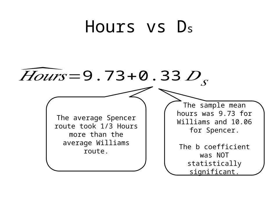
Hours vs Ds
The average Spencer route took 1/3 Hours more than
the average Williams route.
The sample mean hours was 9.73 for Williams and
10.06 for Spencer.
The b coefficient was NOT statistically significant.
�̂�𝑜𝑢𝑟𝑠=9.73+0.33𝐷𝑆
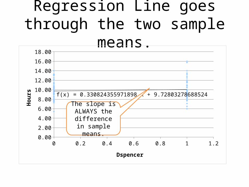
Regression Line goes through the two sample means.
0 0.2 0.4 0.6 0.8 1 1.20.00
2.00
4.00
6.00
8.00
10.00
12.00
14.00
16.00
18.00
f(x) = 0.330824355971898 x + 9.72803278688524
Dspencer
Hours
The slope is ALWAYS the difference in
sample means.

Left-Handers Die Younger, Study Says; Finding That Trait Cuts Lifespan 9 Years Draws Surprise, Skepticism
April 4, 1991 | Malcolm Gladwell | Copyright
• Surveyed next of kin of death records of 2 California counties to determine handedness of the deceased
• Young children and homicide victims were eliminated.• Age of Death (AOD) in years was regressed against DR (1 if right, 0 if left)
Pfeifer’s Trick
• They want you to assume X causes Y.• ALWAYS ask if Y could be causing X.• And then ask if both Y and X are caused
by Z.
Retailers running Oracle are 32% more profitable than their peers.

Female athletes in the nationwide survey were less than half as likely to get pregnant as female non-athletes (5% and 11%, respectively).

People without health insurance more likely to forego routine physical exams
Medical Studies/Trials
Published: Wednesday, 4-Apr-2007

"There is a fairly long history of research showing that early cannabis (marijuana) use is associated with increased risks for later use of so-called 'hard drugs,' but that research is based on the fact that most heroin and cocaine users report first having used cannabis," says lead author Michael T.

Understanding Multiple Regression
• In excel, just highlight multiple adjacent columns of independent (X) variables.
• Regression Output gives a coefficient for each of the X variables.– As well as a standard error, t-stat, p-value
• The multiple regression equation is a PACKAGE DEAL.– You have to use the entire
equation to make valid predictions.

Multiple Regression ExampleMiles Stops Ds Hours331 3 0 10.17206 2 0 8.00221 4 0 8.25
. . . .
. . . .320 9 1 11.50181 9 1 9.50369 7 1 11.75
ANOVA df SS MS F Significance F
Regression 3 367.7819 122.5940 137.1476 1.1566E-39Residual 127 113.5232 0.8939 Total 130 481.3051
Coefficients Standard Error t Stat P-value Intercept 4.2087 0.3009 13.99 1.740E-27 Miles 0.0168 0.0009 17.82 2.386E-36 Stops 0.3234 0.0329 9.84 2.491E-17 Ds -0.9649 0.1788 -5.40 3.231E-07

Multiple Regression
CoefficientsIntercept 4.2087Miles 0.0168Stops 0.3234Ds -0.9649
Intercept 1 1Miles 260 260Stops 6 6Ds 0 1Hours Hat 10.527 9.562
Point forecast for route with 260 miles, 6 stops,
driven by Spencer
Point forecast for route with 260 miles, 6 stops,
driven by williams

Multiple Regression ExampleMiles Stops Ds Hours331 3 0 10.17206 2 0 8.00221 4 0 8.25
. . . .
. . . .320 9 1 11.50181 9 1 9.50369 7 1 11.75
ANOVA df SS MS F Significance F
Regression 3 367.7819 122.5940 137.1476 1.1566E-39Residual 127 113.5232 0.8939 Total 130 481.3051
Coefficients Standard Error t Stat P-value Intercept 4.2087 0.3009 13.99 1.740E-27 Miles 0.0168 0.0009 17.82 2.386E-36 Stops 0.3234 0.0329 9.84 2.491E-17 Ds -0.9649 0.1788 -5.40 3.231E-07
The coefficient of Ds = -0.96
The coefficient of Ds IS significant
Spencer takes LESS time!

What???ANOVA
df SS MS F Signif FRegression 1 3.567397723 3.5674 0.963278 0.3282Residual 129 477.7376725 3.70339 Total 130 481.3050702
Coefficients Standard Error t Stat P-value Intercept 9.7280 0.2464 39.48 0.0000 Ds 0.3308 0.3371 0.98 0.3282
ANOVA df SS MS F Significance F
Regression 3 367.7819 122.5940 137.1476 1.1566E-39Residual 127 113.5232 0.8939 Total 130 481.3051
Coefficients Standard Error t Stat P-value Intercept 4.2087 0.3009 13.99 1.740E-27 Miles 0.0168 0.0009 17.82 2.386E-36 Stops 0.3234 0.0329 9.84 2.491E-17 Ds -0.9649 0.1788 -5.40 3.231E-07
Spencer takes more time.
Spencer takes
less time.
Yes, he does!!!!
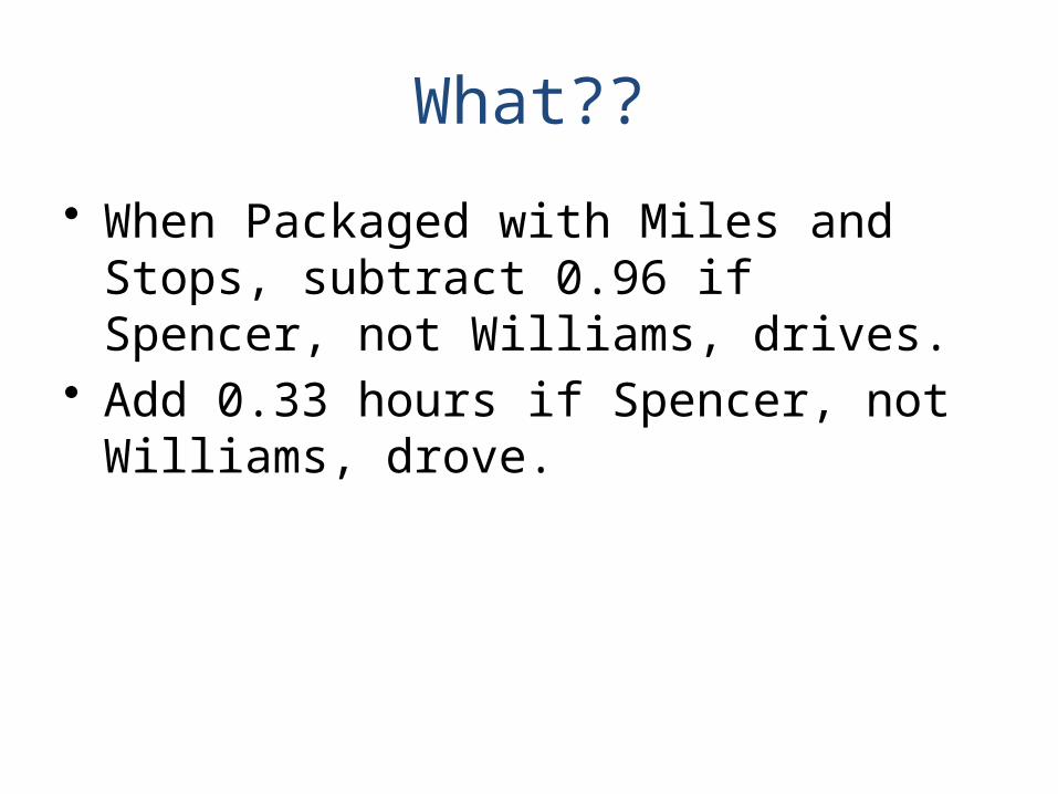
What??
• When Packaged with Miles and Stops, subtract 0.96 if Spencer, not Williams, drives.
• Add 0.33 hours if Spencer, not Williams, drove.
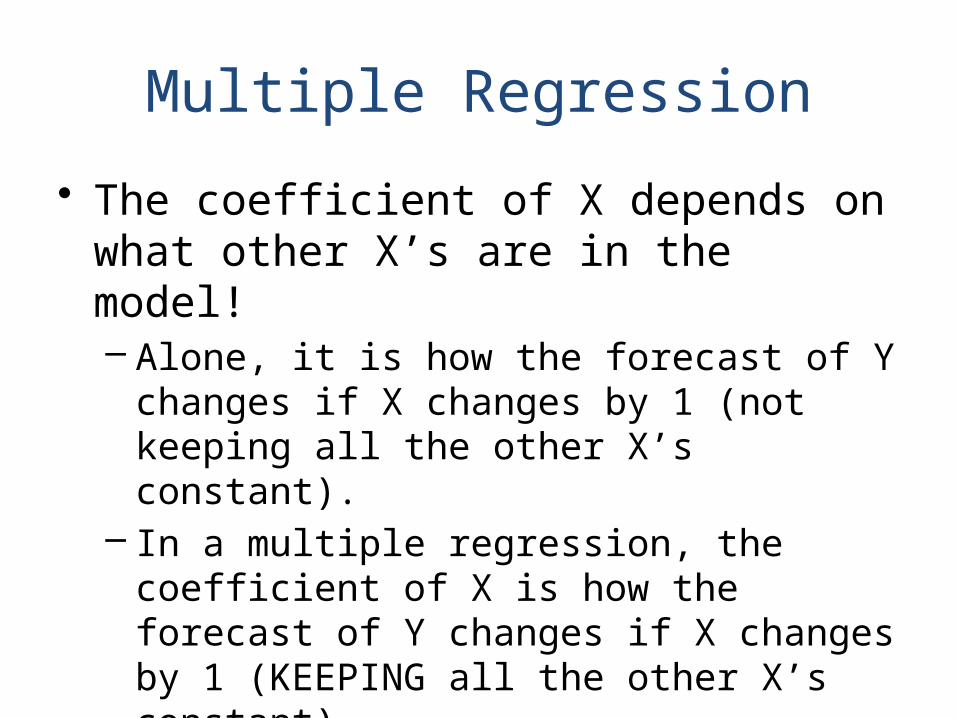
Multiple Regression
• The coefficient of X depends on what other X’s are in the model!– Alone, it is how the forecast of Y changes if X
changes by 1 (not keeping all the other X’s constant).
– In a multiple regression, the coefficient of X is how the forecast of Y changes if X changes by 1 (KEEPING all the other X’s constant).

Multiple Regression
• Allows us to compare Williams and Spencer even though they drove different difficulty routes…if we have the data.
• It is the ANSWER to the tough question.– S hours are higher, but perhaps because S had
higher Miles and Stops– In the multiple regression, we separate the effects of
HOURS, MILES, and DRIVER on Hours.– So the DRIVER gets the coefficient he deserves
because MILES and STOPS get their own coefficients.

Other tough questions?
• Hospital A has a high death rate– But maybe A treats sicker people.
• Private School kids do better in college– But maybe they were smarter to begin with..had access to tutors, etc.
• ND had a great record– But maybe they played an easier schedule
• People who took the expensive drug had better outcomes– But the drug was expensive. Maybe those who took the drug had better
health care, better diets, etc. than those who did not.• People who took the drug (followed instructions) did better.
– But maybe taking the drug is a signal of other things about these people that explain why they did better.
• Women make 70 cents on the dollar compared to men.• Girls who play sports do better in school.
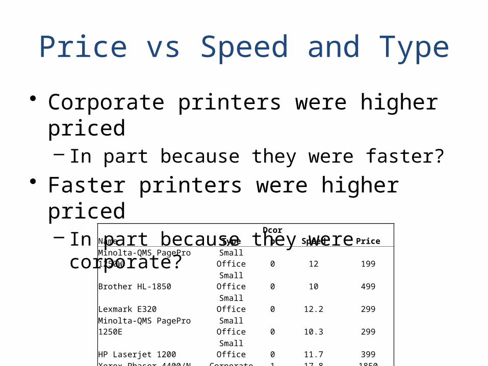
Price vs Speed and Type
• Corporate printers were higher priced– In part because they were faster?
• Faster printers were higher priced– In part because they were corporate?
Name Type Dcorp Speed PriceMinolta-QMS PagePro 1250W Small Office 0 12 199Brother HL-1850 Small Office 0 10 499Lexmark E320 Small Office 0 12.2 299Minolta-QMS PagePro 1250E Small Office 0 10.3 299HP Laserjet 1200 Small Office 0 11.7 399Xerox Phaser 4400/N Corporate 1 17.8 1850Brother HL-2460N Corporate 1 16.1 1000IBM Infoprint 1120n Corporate 1 11.8 1387Lexmark W812 Corporate 1 19.8 2089Oki Data B8300n Corporate 1 28.2 2200
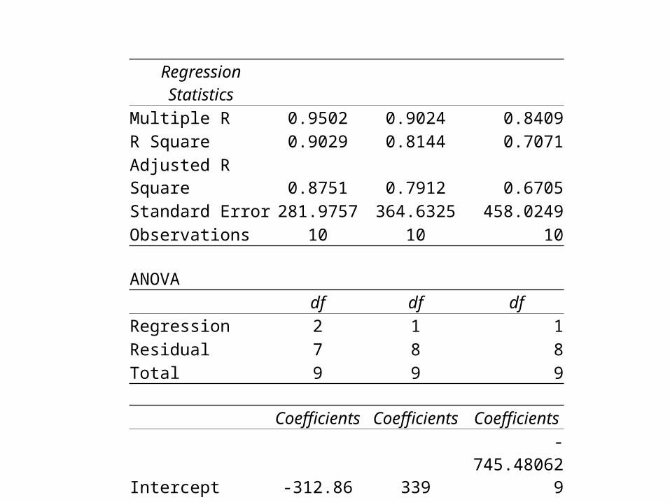
Regression Statistics Multiple R 0.9502 0.9024 0.8409R Square 0.9029 0.8144 0.7071Adjusted R Square 0.8751 0.7912 0.6705Standard Error 281.9757 364.6325 458.0249Observations 10 10 10
ANOVA df df df
Regression 2 1 1Residual 7 8 8Total 9 9 9
Coefficients Coefficients CoefficientsIntercept -312.86 339 -745.480629Dcorp 931.24 1366.2Speed 58.00 117.9173201

Total vs Exams one and two
ID Exam One Exam Two Total1 10 200 2102 20 180 2003 40 120 1604 60 89 1495 80 50 1306 90 60 1507 100 10 110
= 213.1 - 0.96 (Exam One)
= 107.2 + 0.51 (Exam Two)
= ______ + _____ (Exam One) + ______ (Exam Two)
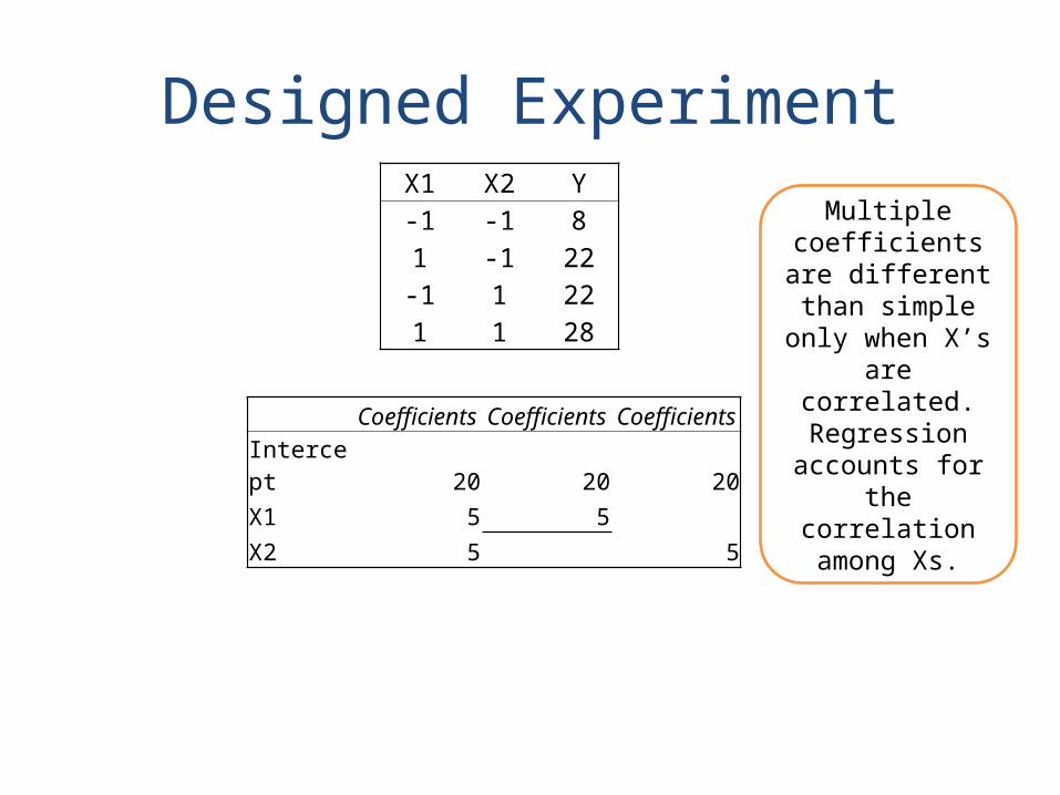
Designed ExperimentX1 X2 Y-1 -1 81 -1 22-1 1 221 1 28
Coefficients Coefficients Coefficients
Intercept 20 20 20
X1 5 5
X2 5 5
Multiple coefficients are different than
simple only when X’s are
correlated.Regression
accounts for the correlation among Xs.

Regression hypothesis TestingSimple
ANOVA df SS MS F Signif F
Regression 1 3.567397723 3.5674 0.963278 0.3282Residual 129 477.7376725 3.70339 Total 130 481.3050702
Coefficients Standard Error t Stat P-value Intercept 9.7280 0.2464 39.48 0.0000 Ds 0.3308 0.3371 0.98 0.3282
H0: b=0
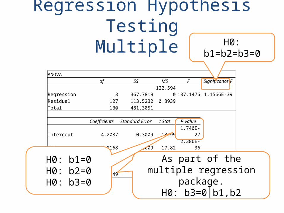
ANOVA df SS MS F Significance F
Regression 3 367.7819 122.5940 137.1476 1.1566E-39Residual 127 113.5232 0.8939 Total 130 481.3051
Coefficients Standard Error t Stat P-value Intercept 4.2087 0.3009 13.99 1.740E-27 Miles 0.0168 0.0009 17.82 2.386E-36 Stops 0.3234 0.0329 9.84 2.491E-17 Ds -0.9649 0.1788 -5.40 3.231E-07
H0: b1=b2=b3=0
H0: b1=0H0: b2=0H0: b3=0
Regression Hypothesis TestingMultiple
As part of the multiple regression package.
H0: b3=0│b1,b2

t-Test: Two-Sample Assuming Equal Variances
Hours(S) Hours(W)Mean 10.05886 9.728033Variance 3.967602 3.399553Observations 70 61Pooled Variance 3.703393 Hypothesized Mean Difference 0 df 129 t Stat 0.981467 P(T<=t) one-tail 0.1641 t Critical one-tail 1.656752 P(T<=t) two-tail 0.328199 t Critical two-tail 1.978524
Miles Stops Hours Ds331 3 10.17 0206 2 8.00 0221 4 8.25 0
. . . .
. . . .320 9 11.50 1181 9 9.50 1369 7 11.75 1
ANOVA df SS MS F Signif F
Regression 1 3.567397723 3.5674 0.963278 0.3282Residual 129 477.7376725 3.70339 Total 130 481.3050702
Coefficients Standard Error t Stat P-value Intercept 9.7280 0.2464 39.48 0.0000 Ds 0.3308 0.3371 0.98 0.3282
H0: μS = μW
H0: b=0
T-test 2-sample ≡ Regression with Dummy
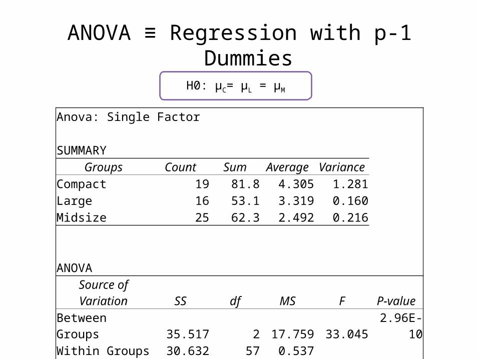
ANOVA ≡ Regression with p-1 Dummies
H0: μC= μL = μM
Anova: Single Factor SUMMARY
Groups Count Sum Average Variance Compact 19 81.8 4.305 1.281 Large 16 53.1 3.319 0.160 Midsize 25 62.3 2.492 0.216 ANOVA Source of Variation SS df MS F P-valueBetween Groups 35.517 2 17.759 33.045 2.96E-10Within Groups 30.632 57 0.537 Total 66.149 59
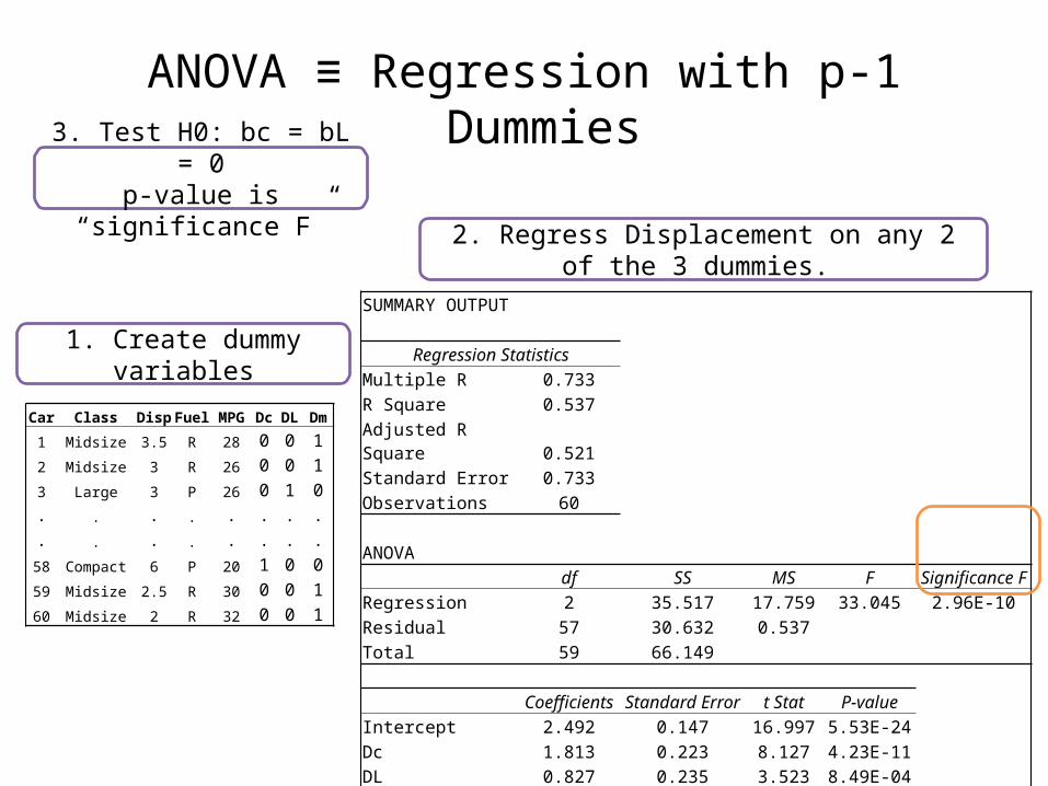
ANOVA ≡ Regression with p-1 Dummies3. Test H0: bc = bL = 0
p-value is “significance F”
Car Class Disp Fuel MPG Dc DL Dm
1 Midsize 3.5 R 28 0 0 12 Midsize 3 R 26 0 0 13 Large 3 P 26 0 1 0. . . . . . . .. . . . . . . .
58 Compact 6 P 20 1 0 059 Midsize 2.5 R 30 0 0 1
60 Midsize 2 R 32 0 0 1
SUMMARY OUTPUT
Regression Statistics Multiple R 0.733 R Square 0.537 Adjusted R Square 0.521 Standard Error 0.733 Observations 60 ANOVA
df SS MS F Significance FRegression 2 35.517 17.759 33.045 2.96E-10Residual 57 30.632 0.537 Total 59 66.149
Coefficients Standard Error t Stat P-value Intercept 2.492 0.147 16.997 5.53E-24 Dc 1.813 0.223 8.127 4.23E-11 DL 0.827 0.235 3.523 8.49E-04
1. Create dummy variables
2. Regress Displacement on any 2 of the 3 dummies.

Class 25
• T-test 2-sample ≡ Regression with Dummy• Understanding Multiple Regression.
– If X’s are correlated (and they usually are), multiple and simple coefficients measure different things.• I hope you know what…
• ANOVA ≡ Regression with p-1 Dummies– Don’t use an index comp=1, mid=2, large=3.– Create p-1 dummies (columns)
EMBS 13.7Pfeifer Note: section 8 (pages 39-42)

Assignment 26Due Wednesday


