University of Illinois at Urbana-Champaign Luthey-Schulten Group NIH Resource for Macromolecular Modeling and Bioinformatics Computational Biophysics Workshop Evolution of Translation Class I Aminoacyl-tRNA Synthetase:tRNA complexes VMD Developer: John Stone MultiSeq Developers Tutorial Authors Elijah Roberts Li Li John Eargle Anurag Sethi Dan Wright Zan Luthey-Schulten A current version of this tutorial is available at http://www.scs.illinois.edu/schulten/tutorials/evolution/
Transcript
University of Illinois at Urbana-ChampaignLuthey-Schulten GroupNIH Resource for Macromolecular Modeling and BioinformaticsComputational Biophysics Workshop
Evolution of TranslationClass I Aminoacyl-tRNA Synthetase:tRNA
complexes
VMD Developer: John Stone
MultiSeq Developers Tutorial Authors
Elijah Roberts Li LiJohn Eargle Anurag SethiDan Wright Zan Luthey-Schulten
A current version of this tutorial is available at
2.4.1 Limitations of sequence data . . . . . . . . . . . . . . . . 242.4.2 Structural metrics look further back in time . . . . . . . . 26
3 Complete Evolutionary Profile of TyrRS 293.1 Expanding the genetic code by engineering TyrRS . . . . . . . . 293.2 Comparing archaeal and bacterial TyrRS:tRNA complexes . . . . 293.3 The structural basis of the altered specificity of the engineered
1.1 The MultiSeq Bioinformatic Analysis Environment
The MultiSeq extension to VMD allows researchers to study the evolutionarychanges in sequence and structure of biomolecules across all three domains of life- Archaea, Bacteria, and Eukarya. For example, one can compare the bacterialsequences and structures of a particular biomolecule to its human counterpartin MultiSeq. MultiSeq contains several metrics for the comparison of sequencesand structures developed by the Luthey-Schulten group [8, 9, 17] in addition tosome of the standard metrics such as percentage identity, sequence similarity,sequence entropy, and RMSD of structures. Of particular note is the inclusionof a recently developed structure-based measure of homology, QH (see AppendixB), that accounts for the effect of insertions and deletions and has been shownto produce accurate structure-based phylogenetic trees. QH is a measure forthe structural similarity between pairs of homologs and is based on a metric,Q, developed by Wolynes, Luthey-Schulten, and coworkers [4], to measure thelocal unfolding of a protein (see Appendix A). In addition to Q, QH has alsogot a gap penalty term that measures how insertions and deletions perturb thealigned core structure of the biomolecule. MultiSeq also includes or allows forthe easy integration of several popular bioinformatics programs, including theSTAMP structural alignment tool, kindly provided by our colleagues Russelland Barton[13], BLAST[1], ClustalW[18], and MAFFT[6]. Our goal is to offerresearchers a complete and user friendly tool for examining the changes in pro-tein sequence and structure in the correct framework of evolution. MultiSeq isan invaluable tool for relating protein structure to function and can be used togeneralize the results to homologous molecules in all three domains of life.
This tutorial showcases the MultiSeq environment and will allow the reader tocombine sequence and structure information into evolutionary profiles used onprotein:RNA complexes in translation [8, 9, 17, 16]. Evolutionary profiles arecompact representative sets that can be used for gene annotation [17], coevolu-tion [12], and energetic analysis [3]. The tutorial is designed such that it canbe used by both new and experienced users of VMD, however, it is highly rec-ommended that new users go through the “VMD Molecular Graphics” tutorialin order to gain a working knowledge of the program. This tutorial should takeabout three hours to complete in its entirety.
1.2 Aminoacyl-tRNA Synthetases: Role in translation
Before beginning the actual tutorial, a small amount of background informa-tion on the cellular translation system may be helpful. The aminoacyl-tRNAsynthetases (aaRSs) are key proteins involved in setting the genetic code in allliving organisms and are found in all three domains of life Bacteria (B), Ar-chaea (A), and Eukarya (E). The essential process of protein synthesis requirestwenty sets of synthetases and their corresponding tRNAs for the correct trans-
1 INTRODUCTION 5
mission of the genetic information. The aaRSs are responsible for loading thetwenty different amino acids (aa) onto their cognate tRNA (tRNA containingthe appropriate anticodon). The formation (See Figure 1) of aminoacyl-tRNA(aa-tRNA) occurs via direct acylation or an indirect mechanism in which theamino acid or amino acid precursor in the misacylated tRNA is modified ina second step. These indirect pathways suggest interesting evolutionary linksbetween amino acid biosynthesis and protein synthesis[11, 14].
Figure 1: (1) The two steps direct acylation of tRNA by glutamyl-tRNA syn-thetase. (a) The glutamate is first combined with an ATP molecule to forman “activated” glutamyl-adenylate and then (b) the adenylate reacts with thetRNA to form the “charged” glutamyl-tRNA. (2) The indirect mechanism forcharging the tRNA. (a) The tRNAGln is mischarged with a glutamate which isthen (b) converted to a glutamine by an amidotransferase.
Each aaRS is a multidomain protein consisting of (at least) a catalytic domainand an anticodon binding domain. In all known cases, the synthetases can bedivided into two types based on homology of their catalytic domains: class I orclass II. Class I aaRSs possess the basic Rossmann fold, while class II aaRSsexhibit a fold that is unique to them and biotin synthetase holoenzyme. Addi-tionally, some of the aaRSs, for example the bacterial leucyl-tRNA synthetase,have an “insert domain” within their catalytic domain (see Figure 2). The tRNAis charged in the catalytic domain and recognition of it takes place through in-teractions with the anticodon loop, acceptor stem, and D-arm of the tRNA (seeFigure 2). In the first part of the tutorial we will examine the evolution of thestructure and sequences of the aaRSs and in the second part, provide a cursoryevolutionary analysis of the tRNA and its recognition elements.
1 INTRODUCTION 6
Figure 2: aaRS:tRNA complex A. A snapshot of GluRS:tRNA:Glu-AMP com-plex (from T. thermophilus; PDB code 1n78) in the active form. The tRNA(shown in yellow) is docked to GluRS (shown as cartoon), and the analog ofGlu-AMP substrate is shown in space-filling representation. The GluRS can bedivided into four parts: the anticodon-binding domain (green), the four helix-junction domain (orange), the CP1 insertion (purple), and the catalytic domain(blue). The catalytic active site is highlighted within the catalytic domain (pinkoval); The three anticodon bases are also highlighted (blue oval). Note that spe-cific contacts between the tRNA and GluRS allow for strategic positioning of thetRNA relative to the enzyme. B. The secondary structure of T. thermophilustRNAGlu. The bases that are essential for tRNA recognition by GluRS areshown in red.
1 INTRODUCTION 7
1.3 Getting Started
1.3.1 Requirements
MultiSeq must be correctly installed and configured before you can begin usingit to analyze the evolution of protein structure. This section walks you throughthe process of doing so, but there are a few prerequisites that must be metbefore this section can be started:
• VMD 1.8.7 beta or later must be installed. The latest version of VMDcan be obtained from http://www.ks.uiuc.edu/Research/vmd/
• This tutorial requires approximately 340 MB of free space on your localhard disk. MultiSeq requires about 500 MB of free space for metadatadatabases.
1.3.2 Copying the tutorial files
This tutorial requires certain files, which are available in the following directoryon the tutorial CD:
/Tutorials/Evolution of Translation Class-I/tutorial-files/
or in the compressed file available for download from the tutorial website.
You should copy this entire directory to a location on your local hard disk. Thepath to the directory must not contain any spaces. For the remainder ofthistutorial, this directory on your local drive will be referred to as TUTORIAL DIR.
1.3.3 Configuring MultiSeq
MultiSeq saves user preferences in a file named .multiseqrc located in yourhome directory. The preferences saved include the location of any local databases,previous search options, and others. When you start MultiSeq for the first time,it will ask you if it is ok to create this file and to specify the directory in whichto look for any metadata databases.
What is metadata? Metadata is a term meaning “data aboutdata”. In MultiSeq the word metadata refers to information aboutthe sequences or structures loaded into the program. MultiSeqknows how to find certain types of sequences or structures in thepublic metadata databases and can display information from themsuch as the species from which the protein originated, the taxo-nomic lineage of the organism, the protein’s enzymatic properties,and even how to find the protein in other databases. You’ll learnmore about how this can be helpful later in the tutorial.
2. Within the VMD main window, choose the Extensions menu, select Analysis→ MultiSeq.
3. MultiSeq will notify you that you must select a directory in which to storemetadata databases. Press the OK button.
4. You will then be prompted to select the metadata directory. If the direc-tory already contains the metadata databases, MultiSeq will use them. Ifnot, MultiSeq will download them into the directory. If you are followingthis tutorial from a CD, choose the TUTORIAL DIR/multiseqdb directoryin the dialog and press the OK button. If you are following from the In-ternet, select the directory where you would like MultiSeq to store thedatabases and press the OK button.
1 INTRODUCTION 9
5. If updates to the metadata databases are available, MultiSeq will presenta dialog showing the available updates and give you the option of down-loading them. Press the Yes button to download the updates. MultiSeqwill ask you to wait while the updates are downloaded, which may take afew minutes depending on the size of the updates and the speed of yourconnection.
6. The MultiSeq Preferences dialog will then appear showing the metadatadirectory and the currently installed databases. Press the Close button tosave these preferences.
1 INTRODUCTION 10
7. The MultiSeq program window will then appear on the screen. The restof the tutorial and exercises will use features from this window, unlessotherwise specified.
Figure 3: The MultiSeq program window
1.3.4 Configuring BLAST for MultiSeq
MultiSeq is now minimally configured. For the purposes of this tutorial, how-ever, some additional functionality is needed. Specifically, the tutorial usesBLAST to perform sequences searches, requiring that a local version of BLASTbe installed.
1 INTRODUCTION 11
What is BLAST and why do I need to install it?BLAST is a software tool available from the NCBI(http://www.ncbi.nlm.nih.gov/BLAST/) that allows you tosearch through a database of sequences and find those that aresimilar to a query sequence or profile of sequences. BLAST allowsfor very rapid searching through a large number of sequences andis widely used in the bioinformatics community. BLAST is typicallyused via one of two methods: online search or local installation.An online search is very simple and requires nothing more than fora user to paste a query sequence into a web page, but the utilityof such a search is somewhat limited. MultiSeq requires a localBLAST installation because it provides additional functionality tothe user not available through an online search.
Follow these steps to install a local copy of BLAST:
1. Create a directory on your local hard disk into which BLAST will beinstalled. Recommended directories are:
• Unix/Linux: /usr/local/blast
• Mac OS X: /Applications/Blast
• Windows: C:\Blast
2. Archives of the BLAST installation for each of the supported platformsare located on the tutorial CD in the directory:
/Tutorials/class-I/blast-install/
or in the compressed file available for download from the tutorial web-site.
Copy the BLAST archive file corresponding to your platform into thedirectory created in the previous step.
3. Extract the archive. On Unix/Linux, use a command such as tar zxvf filename.On Mac OS X and Windows, the archive is a self-extracting executable,so just double-click on it.
4. Next, you must set the BLAST installation location in MultiSeq. Fromthe MultiSeq program window, choose File → Preferences... to bring upthe preferences dialog.
5. Click on the Software button in the upper left portion of the dialog toshow the software preferences.
6. Click on the Browse... button in the BLAST Installation Directorysection and select the directory into which you installed BLAST. Note:
1 INTRODUCTION 12
on Linux and Mac OS X you may have a directory called blast-2.2.13
underneath your installation directory. If so, pick this directory in thebrowse dialog.
7. Press the Close button to save these changes. MultiSeq is now configuredto use your local installation of BLAST.
1 INTRODUCTION 13
1.4 The Glutamyl-tRNA Synthetase:tRNA Complex
1.4.1 Loading the structure into MultiSeq
In order to become familiar with the structural and functional features of theaaRSs, we will first explore the glutamyl-tRNA synthetase (GluRS) as com-plexed with glutamyl-adenylate analog and tRNAGlu (PDB code: 1n78). To dothis:
1. If MultiSeq is not running, start it from within VMD by choosing theExtensions menu and then selecting Analysis → MultiSeq. The MultiSeqprogram window will appear on your screen.
2. Choose the File menu and select Import Data.... The Import Data dialogwill appear.
3. Make sure the From Files radio button is marked and in the Filenamesfield enter the PDB code “1n78”. Click the OK button to have MultiSeqdownload the structure from the PDB website. If you do not have Internetaccess, you can also click on the Browse... button and select the file fromyour local tutorial directory at TUTORIAL DIR/1n78.pdb.
Loading multiple structures. When performing an evolutionaryanalysis, it is common to load numerous structures. MultiSeq makesthis easy by allowing you to select multiple files from your hard diskwhen using the Browse... button on the Import Data dialog. Youcan also have MultiSeq download multiple structures from the PDBby entering them into the Filenames field separated by commas, e.g.“1n78,1asy,1b8a” In addition to PDB structures, MultiSeq allowsyou to download structures directly from the Astral database byentering their SCOP domains. You’ll learn more about Astral andSCOP later in the tutorial.
1 INTRODUCTION 14
You should now have the GluRS:tRNA complex loaded in MultiSeq, as shownin Figure 4. When you load a structure into VMD, MultiSeq represents eachchain of the molecule as a separate row showing the one character code for eachresidue in the columns. In 1n78, the crystallographic unit contains two nearlyidentical complexes. Therefore, you can see two molecules of protein (the Achain and the B chain) and they are named as 1n78 A and 1n78 B in theMultiSeq program window. There are also two molecules of tRNA and named1n78 C and 1n78 D, respectively.
Figure 4: MultiSeq showing the loaded structure 1N78
1.4.2 Selecting and highlighting residues
Click on one of the residues in the sequence named 1n78 A. The residue shouldappear highlighted in both the MultiSeq window and the Open GL display. Ifyou can’t see it in the Open GL display, try changing the representation used forhighlighting the current selection by selecting to the View → Highlight Style →VDW menu option. Notice that MultiSeq also shows the resID of the currentlyselected residue in the status bar at the bottom of the MultiSeq window. Theseare the same resID numbers as in the PDB file and can be very useful duringan analysis. We’ll see how to use them later on.
Now try selecting a larger region by clicking a residue and dragging the mousein the MultiSeq program window. You can also highlight regions in MultiSeqby holding down the Shift and Control keys while clicking with the mouse, asyou would in any other GUI program. These operations are called Shift clickingand Control clicking and will be useful throughout the tutorial. One additionalthing to note is that you can change the color that is used to highlight your se-lection in the Open GL display. Try doing so by selecting the View → Highlight
1 INTRODUCTION 15
Color → Name menu option. Now each atom is colored according to its name.This coloring method can be very helpful when looking at specific atomic levelinteractions between residues, such as hydrogen bonds.
1.4.3 Domain organization of the synthetase
All of the aaRSs are multidomain proteins, but the exact number and fold ofeach domain is specific to each synthetase. GluRS has a catalytic domain (com-prised of residues 1–79 and 181–306), a four helix-junction domain (residues307–374), an anticodon-binding domain (residues 375–468), and a CP1 inser-tion (residues 81–186, CP1 referred to connected-peptide 1). Interestingly, theCP1 insertion interrupts the sequence of the catalytic domain. Try selectingeach domain one at a time. You can select two non-contiguous regions in Multi-Seq by clicking the first residue of the first region, Shift clicking the last residueof the first region, Control clicking the first residue of the second region, andfinally Control-Shift clicking the last residue of the second region.
The anticodon for glutamate is comprised of C534, U535, and C536. Selectthese bases in Multiseq and they will be highlighted. Note how the anticodon-binding domain of the enzyme attaches itself to the anticodon in the tRNA;zoom in on the anticodon. The CUC anticodon decodes GAG codon, whichencodes glutamate. You will examine the tRNA in more detail in Section 4.
1.4.4 Nearest neighbor contacts
When analyzing protein structures, it is often desirable to know what residuesare in contact with each other. Here we will identify those residues in the GluRSthat recognize the anticodon. To make this process easier, MultiSeq provides afunction that allows you search for residues in contact with a selected region.To do this, first click the checkbox to the left of the name of sequence 1n78 A.The sequence should appear checked as shown below.
This is called marking a sequence; multiple sequences can be marked in Multi-Seq at the same time. MultiSeq allows you to limit the scope of many operationsto sequences that are marked. Now, with the three anticodon bases (bases C34,U35, and C36) highlighted in MultiSeq, select the Search→ Select Contact Shells
1 INTRODUCTION 16
menu option. The Select Contact Shells dialog will appear. Change the scope ofthe search to be only the marked sequences by selecting the Marked Sequencesradio button, change the contact distance to be 3.0 A, and then and press theOK button.
Figure 5: Select Contacts Shells dialog
The residues of the protein that are within 3.0 A of the anticodon are selectedin both the MultiSeq window and the Open GL display, as shown in Figure 6.They include R358, R417, R435, L442 and T444. As you may noticed, manyof them are positively charged residues, which can stabilize the RNA:proteininteraction by electrostatic forces. Among these residues, R358 is particularlyinteresting: it is responsible for discriminating tRNAGlu and tRNAGln[15]. Alsonotice the π - cation interaction between residue R435 of the synthetase andbases U535 of the tRNA. What other types of interactions between the proteinand tRNA can you recognize?
Use VMD to zoom in on the active site within the catalytic domain; you maywant to rotate the molecule to get the best view possible. Note how the ac-ceptor stem of the tRNA bends into the active site of the GluRS. Select theresidue of position 469 in chain A. This “mysterious” residue is the analog ofglutamyl-adenylate. The formation of the glutamyl-adenylate comes from oneglutamate molecule and ATP; this adenylated species is “activated” and thentransferred to the cognate tRNA with energy provided from the hydrolysis ofthe adenylate complex to AMP. Also note how the architecture of the activesite prohibits the diffusion of this activated amino acid out of the active site;the glutamyl-adenylate is trapped between the catalytic domain and the tRNA.
1 INTRODUCTION 17
Figure 6: Residues of GluRS (green ) within 3.0 A of the anticodon (yellow)
The chemistry of aaRSs Explore the active site of the GluRS-tRNAcomplex in a similar way to what you did above for the anticodonregion and answer the following questions: What step of the reactionshown in Figure 1 does this structure represent? What are thesubstrates? What products are synthesized by this reaction? Whatpart of the tRNA is involved in this reaction? What part of theprotein is involved?
1 INTRODUCTION 18
Where does the tRNA go once it is “charged” with its aminoacid? At the ribosome, the anticodon of the charged tRNA ismatched to the mRNA codon. Then the tRNA is deacylated withthe amino acid being added as the next residue in the nascent pro-tein chain.
Send the tRNA off to the ribosome yourself by deleting the molecule before youbegin the next part of the tutorial. You can do this by selecting the File → NewSession menu option.
2 EVOLUTIONARY ANALYSIS OF AARS STRUCTURES 19
2 Evolutionary Analysis of aaRS Structures
In this part of the tutorial, we will use MultiSeq to align the catalytic domainsof 31 class I aaRS structures, representing 11 different specificities from each do-main of life. The catalytic domain of each structure has been directly extractedfrom the ASTRAL database, which contains the structures of each of the pro-teins’ domains. This part of the tutorial will emphasize both structural andsequence based analyses of the aaRSs and ultimately create a phylogenetic treeillustrating the evolution of the protein family. A sequence based phylogeneticanalysis can be used to study recent phylogenetic events. However, sequencealignments are less reliable as the sequence identity reduces below 30% (twilightzone). On the other hand, a structural phylogenetic tree allows examination ofmore distant evolutionary events such as when specificity was being acquired.We use as a reference for all trees the universal tree developed by Carl Woeseusing 16S ribosomal RNAs (Figure 7).
Figure 7: Universal tree of life
2.1 Loading Molecules
To further explore aaRSs, we will now examine the catalytic domain of 31 ClassI aaRS structures in MultiSeq. Before we begin, make sure you have deletedany molecules in the MultiSeq program window.
1. Select the File→Import Data item in the Main MultiSeq window. We willbe importing Data From Files. Make sure From Files is selected.
2. Hit the Browse button. A file browser window will appear. Navigate thefile browser to the TUTORIAL DIR/class-1-synthetases directory.
2 EVOLUTIONARY ANALYSIS OF AARS STRUCTURES 20
3. There are 31 PDB files you want to load from the directory. You may needto change the filename filter to allow for selection of PDB files1. Select allof the files by clicking on the first file with your mouse and holding downthe shift key and then selecting the last file.
4. Hit the OK button in the file browser window.
5. Notice that all of the file names will appear in the field Filenames. If thislooks correct hit the OK button at the bottom of the Import Data dialog.
Since there are several files, it will take VMD about a minute to fully load themolecules. Once the molecules are in VMD and MultiSeq, you will see a 3Drepresentation in the OpenGL display and sequence information in the SequenceDisplay of the main MultiSeq window.The molecules will appear in the OpenGL display window. We will now walkthrough the steps for aligning these molecules.
What is the ASTRAL database? The ASTRAL database(http://astral.berkeley.edu) is a compendium of protein domainstructures derived from the PDB database. It divides each proteinstructure into its domain components defined by SCOP. For exam-ple, GluRS is divided into two separate PDB files: one containingthe catalytic domain, and one for the anticodon binding domain.The names of the files contain the PDB code, the chain name, andnumber, which corresponds to the structural domain. For example,the anticodon binding domain for one of the GluRS-tRNA complexis: d1j09a1.
2.2 Multiple Structure Alignments
Next we will structurally align the molecules:
1. Go to the MultiSeq program window and select Tools in the top pull-downmenu.
2. Then click on Stamp Structural Alignment. A new window entitled StampAlignment Options will appear with default settings (see Figure 8).
Perform the alignment by hitting the OK button. Once this step is complete,you will be able to view the structural alignment in both the OpenGL Displaywindow and the main MultiSeq Window.
If you would like more information about STAMP parameters, please refer tothe STAMP manual.2
1Note these commands for selecting all of the PDB files may differ on various operatingsystems. Select all of the files as appropriate for your operating system.
2The STAMP manual is available at http://www.compbio.dundee.ac.uk/manuals/stamp.4.2/stamp.html
2 EVOLUTIONARY ANALYSIS OF AARS STRUCTURES 21
Figure 8: Stamp Alignment Options Window
How molecules are aligned in a multiple structural alignmentMultiSeq uses the program STAMP to align protein molecules.The STAMP algorithm minimizes the Cα distance between alignedresidues of each molecule by applying globally optimal rigid-bodyrotations and translations. Also, note that you can only performalignments on molecules that are structurally similar. If you tryto align proteins that have no common substructures, STAMP willhave no means to align them. If you would like further informationabout how the alignment occurs, please refer to the STAMP manual
2.3 Structural Conservation Measure: Qres
MultiSeq features various coloring metrics for protein analysis. When applied tostructures, the coloring is displayed in both the OpenGL display and the mainMultiSeq window. Qres is the coloring metric for structure similarity in multiplealignment of structures. Determining structure conservation is one method inevolutionary analysis that helps us understand what regions of a protein, or inthis case what structural elements of the catalytic domain of aaRSs, are con-served across all specificities. In this tutorial we use the RGB (red-green-blue)color scale instead of the default RWB (red-white-blue) so that only gaps appearwhite in the alignment editor.
2 EVOLUTIONARY ANALYSIS OF AARS STRUCTURES 22
To change the color scale:
1. From the VMD Main window select Graphics → Colors... to bring up theColor Controls window.
2. In the Color Controls window select the Color Scale tab.
3. Choose RGB from the Method pick list.
4. Close the Color Controls window.
What is Qres? To answer this question we first must consider“What is Q?” Q is a parameter borrowed from protein folding thatindicates structural similarity. Traditionally, Q has meant “the frac-tion of similar native pairwise distances” between aligned residues intwo proteins, or in two different conformational states of the sameprotein. When Q = 1, it indicates that the structures are identical.When Q has a low score (0.1), it means that few pair distances aresimilar to their native values, or, in other words, the structures donot align well. Homologs typically have Q≥0.4. Qres is the contri-bution from each residue to the overall average Q value. For moreinformation see Appendices A–C
Qres, is accessed by:
1. Click on the View menu in the MultiSeq program window.
2. Make sure Coloring → Apply to all is checked and select Coloring → Qres.
Look at the OpenGL Display window to see the impact coloring by Qres hasmade on the molecules.
You will probably notice that several regions within the interior of the alignedmolecules have turned green. Rotate the molecule to see how much of it hasturned green. Green indicates that the molecules are somewhat structurallyconserved at those points; while blue indicates identical structures (Qres = 1)and red for unaligned parts (Qres = 0), which often correspond to insertionsthat are unique to one specificity. For homologous proteins, Qres ≈ 0.7, hencethey are colored bluish green.
You can also view secondary structure information derived from the crystalstructures. In a structural alignment, α-helices and β-strands from a givenprotein should align with similar elements in the other proteins.To view the secondary structures for the sequences in your alignment:
1. In the MultiSeq window select the sequences by clicking the name of thetopmost sequence and then shift-clicking the name of the bottom sequence.All sequences should appear highlighted.
2 EVOLUTIONARY ANALYSIS OF AARS STRUCTURES 23
Figure 9: The catalytic domain colored by Qres.
2. Click the r box to the right of one of the sequence names and chooseSecondary Structure from the popup menu.
You should now be able to see picture representations of α-helices (wavey rib-bons), β-strands (fat arrows), and coils (thin lines). Scroll through the align-ment and look at how the secondary structure elements align. To view thesequences again follow the above instructions but choose Sequence from thepopup menu.
Core Structure Now that we have observed the structural conserva-tion patterns, go back to the main MultiSeq window and see wherethe coloring of the core begins and ends. Since all the class I aaRSshare a homologous core, you would expect the core residues shouldhave a high Qres value and have a green color in the alignment.Using the side-scroll on the bottom of the main MultiSeq window,you can see the core residues begins at about position 160 and endsaround 1150 in the alignment (notice that the position number inthe alignment is not always the same as the residue number in eachsequence, since the alignment contains gaps). However, not allsequences in this region are core residues, many of them are inser-tions, which are characterized by a low Qres value and thus appearto be red in the alignment. For example, there is a long insertionbetween position 830 to 880 for entry d1wkba3, which correspondsto Pyrococcus horikoshii LeuRS.
2 EVOLUTIONARY ANALYSIS OF AARS STRUCTURES 24
2.4 Structure Based Phylogenetic Analysis
2.4.1 Limitations of sequence data
In this section we will look at the phylogenetic history of the class I aaRS struc-tures. Most common methods of phylogenetic analysis use only informationderived from the sequences to build the tree. However, the following two rea-sons restricted the application of these methods to highly divergent sequencedata. First, a set of highly divergent sequences may not generate a reliablealignment, this is true for the case of class I aaRS, in which we have to appliedthe structural alignments, as we did in previous part. Second, many of theproteins we are looking at diverged before the last universal common ancestralstate (LUCAS), and have evolved independently since then. Consequently, theyhave a very low level of sequence identity. In fact, many of them have no moresequence relation than would be expected at random (8–10%). This is calledthe “midnight zone” of sequence identity and makes phylogenetic reconstruc-tion using sequence metrics unreliable for very distantly related proteins. Todemonstrate the second point, construct a sequence based phylogenetic tree ofthese aaRSs by following these steps:
1. In the MultiSeq program window, select the Tools → Phylogenetic Treemenu option.
2. The Create Phylogenetic Tree dialog will appear. Select Sequence treeusing Percent Identity as the type of tree to construct and press the OKbutton.
Calculating phylogenetic relationships. The phylogenetic trees inMultiSeq are all distance based trees. This means that they arecalculated by using a pairwise metric (e.g. percent identity or QH)to build a matrix comparing all possible pairs and then transform-ing this distance matrix intoa tree. To do this, MultiSeq uses twotreeing methods: UPGMA (Unweighted Pair Group Method withArithmetic mean) and Neighbor-Joining. Other methods, such asMaximum Likelihood or Maximum Parsimony, may give more accu-rate results, but are generally much more computationally intensive.MultiSeq does not support computing trees this way, but will allowyou to view them after they have been computed. Look up the de-tails of these four tree computation methods on the Internet. Whichone would you choose to use?
A phylogenetic tree based on percent sequence identity of the proteins will becalculated and drawn, as shown in Figure 10. Select View → Leaf Color →Taxonomy->Domain of Life and then View → Leaf Text → Enzyme->Name toshow more information in the tree viewer.
2 EVOLUTIONARY ANALYSIS OF AARS STRUCTURES 25
How to read a phylogenetic tree. MultiSeq shows phylogenetictrees as dendrograms. A dendrogram represents the distance be-tween any two nodes of the tree as the total horizontal distancetraversed to get from one node to the other. In Figure 10, for ex-ample, the distance traversed to get from d2ts1 to d1jila is 0.38,or twice the distance to their closest common parent node. In thisexample, that distance represents 62% identity between the two se-quence. The distance between any two nodes is shown in the treestatus bar when you click on the first node and then Shift click onthe second node.
It is important to examine the phylogenetic tree we have built. At first glance,you may notice that many aaRSs with same specificity are grouped together,which is quite reasonable. The IleRS, LeuRS, ValRS and MetRS are groupedclose to each other. Similarly, the GluRS and GlnRS, the TyrRS and TrpRSform two individual groups. This observation is consistent with the detailedclassification of class I aaRSs[5]. Yet, a closer look brings more questions. Forexample, the ValRS groups within two IleRSs, which should form a monophyleticgroup by themselves. Also, you should notice that many of the branch pointslie below 10% sequence identity (0.05 on the dendrogram). These branch pointsare unreliable as discussed above. To resolve these problems, we are going tobuild a structure based phylogenetic tree.
2 EVOLUTIONARY ANALYSIS OF AARS STRUCTURES 26
2.4.2 Structural metrics look further back in time
In order to reliably compare such distantly related proteins, we need a metricthat is based on a property of the protein that is more highly conserved throughevolutionary time. As structure has been shown to be more conserved than se-quence, a structural metric fits this description. MultiSeq supports using QH
and RMSD between aligned proteins to construct structural phylogenetic trees.QH is detailed in the paper titled “Evolutionary profiles derived from the QRfactorization of multiple structural alignments gives and economy of informa-tion” located in the tutorial distribution at:
TUTORIAL DIR/papers/odonoghue JMB 2005.pdf
Generate a QH structural phylogenetic tree of the aaRSs by performing thefollowing:
1. Select the Tools → Phylogenetic Tree menu option.
2. In the Create Phylogenetic Tree dialog select the All Sequences radio but-ton.
3. Make sure only the Structural tree using QH checkbox is checked and pressthe OK button.
MultiSeq calculates and displays the QH tree for the selected structural regions.Comparing this tree (shown in Figure 11) to the sequence tree generated ear-lier, the structure based tree retains most of the correct features within a givenspecificity. The structure based tree also makes some improvements on the phy-logenetic relationship. For example, in the structure based tree, two IleRSs aregrouped within a monophyletic group. You may also notice how the branchpoints are much more evenly spaced, not bunched together on the left of thetree. This indicates that the phylogenetic history is recorded in the structures,and it is elucidated when using the structural tree. However, the evolutionaryrelationship between TrpRS and TyrRS is still not well resolved. To overcomethat problem, we need to compare the full length TrpRS and TyrRS3.
Our current tree is slightly different from the one we showed in the MMBRpaper (page 561), since we are using different structure sets. As you can see,the old dataset contains fewer structures. Our current one is more balanced,less redundant, also has more representatives from the specificities/domains oflife that were not resolved earlier.
3That is how we solve the problem in the MMBR paper.
2 EVOLUTIONARY ANALYSIS OF AARS STRUCTURES 27
Figure 10: Percent identity sequence phylogenetic tree of 31 diverse aaRS struc-tures. Note here that some aaRS entries do not contain information about theirspecificities and species names. We add the information manually (shown inparenthesis).
2 EVOLUTIONARY ANALYSIS OF AARS STRUCTURES 28
Figure 11: QH structural phylogenetic tree of 31 diverse class I aaRS structures.For those ASTRAL structures not present in the metadata, we provided thespecificity and the species name of each aaRS manually (shown in parenthesis).
3 COMPLETE EVOLUTIONARY PROFILE OF TYRRS 29
3 Complete Evolutionary Profile of TyrRS
3.1 Expanding the genetic code by engineering TyrRS
So far we have investigated only structures of the catalytic domain of the class ItRNA synthetases. Further analysis of the catalytic domain requires looking atsequences as well. For this tutorial we will be concentrating on one specificityfrom the class I aaRSs, the tyrosyl-tRNA synthetases.
Methanococcus jannaschii TyrRS is the first synthetase that has been en-gineered to incorporate an unnatural amino acid into protein in E. coli [19].The overall strategy is to engineer an aaRS that can specifically aminoacylatea tRNA with an unnatural amino acid, and this tRNA (the suppressor tRNA)can deliver the amino acid to a specified position (an amber stop codon) on anygene. Schultz and his colleagues chose TyrRS for this purpose due to severalreasons. First of all, archaeal and bacterial TyrRS recognize different parts ontRNA. In particular, the archaeal TyrRS recognizes the C1-G72 base pair, thediscriminator base A73, and the anticodon loop; while the bacterial TyrRS relieson the G1-C72 base pair, A73, the anticodon loop as well as the long variablearm. This makes the bacterial TyrRS unable to charge archaeal tRNATyr andvice versa. Secondly, TyrRS can recognize the suppressor tRNA, largely due tothe similarity between the tyrosine codons (UAU and UAC) and the amber stopcodon (UAG). Finally, TyrRS will not hydrolyze the charged unnatural aminoacid.
The names of stop codons Stop codons were historically givenmany different names as they each corresponded to a distinct class ofmutants. Amber mutations were the first set of nonsense mutationsto be discovered, within bacteriophage T4. It is named after thegraduate student, Harris Berstein, who first isolated these mutants(Berstein means ”amber” in German). The ochre and opal mutantswere isolated later, and their names were given to color names tomatch the amber mutants. It turned out later that the amber,orche, and opal mutants corresponds to the mutations to the stopcodon ”UAG”, ”UAA” and ”UGA”, respectively.
3.2 Comparing archaeal and bacterial TyrRS:tRNA com-plexes
First, we start a new session of Multiseq and load the structure of the M. jan-naschii TyrRS (PDB code 1J1U)[7] by importing the file TUTORIAL DIR/1j1u dimer.pdb
into Multiseq. Note here although TyrRS forms a homodimer, the original PDBfile contains only one molecule of TyrRS and one molecule of tRNA. For thepurpose of the tutorial, we have built the dimer complex based on crystallog-raphy symmetry (P31 2 1 for 1J1U) by Swiss-PDB viewer4. Try to color the
4http://us.expasy.org/spdbv/text/download.htm
3 COMPLETE EVOLUTIONARY PROFILE OF TYRRS 30
molecules by chain. To do that:
1. Open the Graphical Representations panel in VMD.
2. Change the color in the Color ID list for each chain so that they havedifferent colors.
You can clearly see that a tRNA molecule spans the two subunits of the homod-imer: the acceptor stem of the tRNA molecule interacts with one subunit; whilethe anticodon loop is recognized by the other. You might also notice that thecrystal structure is missing some important parts of the TyrRS:tRNA complex,for example, the CCA end in the tRNA and the KMSK loop in the TyrRS. Thisis probably because that these regions are flexible in the absence of ATP.
How M. jannaschii TyrRS specifically recognizes the C1-G72base pair. Try to use the method we described in the introduc-tion to find out the residues that are responsible for the specificity.Hint: you may first select the C1-G72 base pair in Multiseq and findresidues in its contact shell.
Next, we will examine the structure of Thermus thermophilus TyrRS (PDBcode 1H3E)[20], which represents the bacterial type TyrRS. As above, we gen-erated the homodimer of the TyrRS:tRNA complex based on crystallographysymmetry. Here, you can load the file TUTORIAL DIR/1h3e dimer.pdb into Mul-tiseq. You will notice that the T. thermophilus structure is significantly differentfrom the archaeal structure: a long arm of tRNA (the variable arm) protrudesoutward, and extensive contacts are formed between this part and protein. Thearchaea tRNATyr, which does not have the long variable arm, will not bindstably to the bacterial TyrRS. You can also try to find how the G1-C72 basepair is specifically recognized by T. thermophilus TyrRS.
3.3 The structural basis of the altered specificity of theengineered TyrRS
In Schultz’s paper, he and his colleagues reported that by introducing fourpoint mutations (Y32Q, D158A, E107T, L162P), they can convert the TyrRS tospecifically aminoacylate O-methyl-tyrosine. Subsequently, the crystal structureof the engineered TyrRS was solved[21]. In this section, we try to understandthe structural basis of the altered specificity. To do this:
1. Delete all the old structures in the MultiSeq program and load three newstructures: 1u7d (apo wild-type M. jannaschii TyrRS), 1u7x (apo engi-neered M. jannaschii TyrRS), and 1h3f (T. thermophilus TyrRS boundwith a tyrosine analog).5
5As you may notice, the protein structure of 1h3f seems to contain two separate proteins.This is an artifact due to some missing residues in the crystal structure.
3 COMPLETE EVOLUTIONARY PROFILE OF TYRRS 31
2. Delete the B chain for 1u7d and 1u7x, as well as the A chain for 1h3f.
3. Align these three structures by STAMP structural alignment. Color thestructure by Qres. You should see that the majority of the catalytic siteis blue, indicating a good alignment among these structures.
4. Select the last residue in 1h3f that is shown as a X. This is tyrosinol, ananalog of tyrosine.
5. Select the four mutated residues: Y32, D158, E107 and L162 in 1u7d andtheir counterparts in 1u7x.
You can see that Y32Q and D158A enlarge the amino acid binding pocketdirectly, although the other two mutations are not close to the binding pocketand their mechanisms are not clear.
3.4 Evolutionary Profile of TyrRS
3.4.1 Importing the archaeal sequences
In this section, we will closely examine the difference between the archaealand bacterial TyrRS as well as their evolutionary relationship by generating anevolutionary profile. To do this in MultiSeq, we will perform a BLAST search ofa TyrRS structure from each domain of life against the Swiss-Prot database oneat a time, starting with the Archaea. Doing the search separately within onedomain of life will allow us to be more sensitive in finding only TyrRS sequences.To run the search:
1. In the MultiSeq program window select the 1U7D A sequence as our sourceby marking it.
2. Click the File → Import Data menu option.
3. The Import Data dialog will appear. Select the From BLAST Search radiobutton.
3 COMPLETE EVOLUTIONARY PROFILE OF TYRRS 32
4. In the Search Profile section select the Marked Sequences radio button.
5. Next to the Database field, press the Browse... button and select the fileTUTORIAL DIR/swiss-prot/uniprot sprot to search over the Swiss-Protdatabase.
6. Set the E Score to be e-20 and the number of Iterations to (1) one6.
7. Now click the OK button. The search may take a minute or two.
E value The Expect value (E value) represents the proba-bility that a certain match or a better one would be ex-pected to occur purely by chance in a search of the entiredatabase. Thus, the lower the E value, the greater the simi-larity between the input sequence and the match. For a morecomprehensive description, you may read the following website:http://www.ncbi.nlm.nih.gov/BLAST/tutorial/Altschul-1.html
6We usually set the E value threshold as e-3 or even higher. Here, the extremely low Evalue is used to screen out TrpRS sequences.
3 COMPLETE EVOLUTIONARY PROFILE OF TYRRS 33
Figure 12: Blast Search Results Dialog
When the search is complete, a new dialog called BLAST Search Results appears(see Figure 12). As you may have noticed, 329 sequences were found by BLAST.To restrict the results to only the Archaea, do the following:
1. In the Filter Options section and in Domain list, unselect the All list itemby clicking on it and the select the Archaea list item.
2. Press Apply Filter button.
The dialog now displays only the 39 sequences from the domain Archaea. Pressthe Accept button at the bottom of the window to bring these sequences intoMultiSeq.
3.4.2 Now the other two domains of life
Since there are no eukaryal cytoplasmic TyrRS structures available, we will stilluse the archaeal one as the seed of BLAST search. This time, select Eukaryotafrom the Domain list. You will find five eukaryal TyrRS. Bring all of them intoMultiseq.
Now perform the same search for the bacterial structure by unmarkingd1U7D A, marking d1h3f B, and then repeating the above steps with E Score set
3 COMPLETE EVOLUTIONARY PROFILE OF TYRRS 34
to e-5 . Be sure to select Bacteria in the Domain list this time. This will bring in382 sequences. You can immediately tell that the Bacteria are over-representedin the sequence databases7, and if you examine these sequences more carefully,you will notice that many of them are highly similar. Eliminating this biasand redundancy is important in obtaining good evolutionary profile and will bediscussed later in more detail. Here, we first use the binary QR to screen outmost of the redundant sequences8. To do this:
1. In the Filter Options section and in Percentage to return line, scroll theindex to 20. This will give you 54 sequences.
2. Press Apply Filter button.
3. Press Accept button.
After you obtain the bacterial TyrRS sequences, you should make sure thatall their names start with SYY. Sometimes you may retrieve TrpRS sequences,which start with SYW. These sequences should be excluded in the followinganalysis.
3.4.3 Organizing Your Data
At this point you may be overwhelmed by all of the data in the MultiSeq programwindow. In order to construct an evolutionary profile and observe sequencesignatures specific to a particular domain of life, MultiSeq has various toolsthat help in the organization of data. One such tool allows you to automaticallygroup sequences and structures by domain of life:
1. Select the Options→ Grouping→ Taxonomy... menu option. A new dialogcalled Group Sequences by Taxonomy appears.
2. Choose All Sequences..
3. Select domain as the level by which to group the data.
4. Press the OK button.
The sequences will now be grouped in the MultiSeq program window by domainof life.
7Here we have used only a subset of the Swiss-Prot database. In reality, you will obtaineven more sequences.
8Strictly speaking, the QR algorithm should be performed after the sequence alignment ofall the available sequences. However, an alignment and the complete Sequence QR factoriza-tion of about 300 sequences will take a very long time. So, in order to finish the sequencealignment in a reasonable amount of time, we applied the binary QR method. In the binaryQR method, all amino acids are encoded in a single dimension unlike Sequence QR which hasa dimension for every amino acid. The second dimension in binary QR encodes the gap posi-tions in the alignment. Binary QR calculates the most representative set of protein sequencesbased on the pattern of gaps in the BLAST alignment.
3 COMPLETE EVOLUTIONARY PROFILE OF TYRRS 35
3.4.4 Aligning to a Structural Profile using ClustalW
Finally we have a set of sequences and structures of the catalytic domain ofthe tyrosyl-tRNA synthetase loaded. In order to analyze the group as a whole,however, the entire set must be aligned. While sequence alignment methodsgenerally work well for closely related proteins, this set is too diverse to yielda good sequence alignment. What we will do instead is use the structuralalignment, which is more accurate for distant proteins, to guide the sequencealignment. Here, we will build a more reliable structural alignment based on sixTyrRS structures. The following steps will walk you through that process:
1. Delete all the loaded TyrRS structures.
2. Load all six PDB files from TUTORIAL DIR/tyrRS/. They are 1vbma(Escherichia coli TyrRS), 1u7da (Methanocaldococcus jannaschii TyrRS,2dlca (Saccharomyces cerevisiae TyrRS), 2cyba (Archaeoglobus fulgidusTyrRS), 2cyaa (Aeropyrum pernix TyrRS) and 1h3fa (Thermus thermophilusTyrRS), respectively.
3. These structures should appear in a new group called VMD ProteinStructures, rename this group as Structures by right-click the groupname and select Rename Group..., enter Structures as the name of the newgroup and press OK.
4. Mark all six structures.
5. Use STAMP to align the marked structures using the Tools → StampStructural Alignment menu option.
6. Check the quality of the structural alignment by coloring the residues byQres. You should notice that these structures can be aligned very well.
7. Unmark the structures and mark all of the sequences in the Archaea,Bacteria and Eukaryota. Now, we will align all the sequences to thestructural alignment. We would like to emphasize here that inresearch, it is better to align sequences from each domain oflife separately to generate sequence profiles first and then alignthese sequence profiles using the structural alignment as a guide.
8. Remove all gaps from the marked sequences using the Edit → RemoveGaps... menu option.
9. Bring up the ClustalW dialog by choosing Tools → Sequence Alignmentfrom the menu.
10. In the dialog, select Profile/Sequence Alignment and tell ClustalW to alignmarked sequences to the Structures group.
11. Align the sequences to the structural profile by pressing the OK button.ClustalW will take a minute to perform the alignment.
3 COMPLETE EVOLUTIONARY PROFILE OF TYRRS 36
You now have a structure based alignment of the tyrosyl-tRNA synthetase. Trycoloring it according to sequence identity by choosing View→ Coloring→ Applyto All and then View → Coloring → Sequence Identity (shown in Figure 13).Play around with the other coloring metrics. Do you understand what they alldo? Also try coloring by groups independently. What additional insight do youthink you can gain by doing so?
Figure 13: MultiSeq showing all sequences colored by sequence identity
3.4.5 Curating the sequence alignment
After you obtained the sequence alignment, it is important to check it manually.Even the best alignment algorithm will make errors, especially if the sequencesare divergent. A basic principle for alignment curating is that those functionallyimportant motifs should be aligned (here, the HIGH and KMSK motifs). Asyou noticed in Figure 13, the HIGH motif is aligned well9. However, for some
9Note there is some variations among the HIGH motif. For example, you can see HLGH,HVGH in the alignment.
3 COMPLETE EVOLUTIONARY PROFILE OF TYRRS 37
of the archaeal TyrRS, the KMSK motif (around position 310) are not aligned.To overcome this problem, you have to edit the sequence alignment manuallyby inserting some gaps:
1. Choose Edit → Enable editing → Gaps Only from the menu.
2. Align KMSK region by adding and deleting gaps. For example, for the en-try SYY AERPE, you need to delete five gaps right before the sequenceEIDDVLAEVKMSKS by pressing the “delete” button, and add fivegaps after it by simply pressing space button. By doing that, we can alignKMSK motif and still maintain the rest part of the alignment. Try toalign the rest of KMSK motifs. The final alignment should look similaras Figure 14
3. Color the sequences by Sequence Identity again. The KMSK region shouldappear blue or green.
Conservation of important residues responsible for tyrosinerecognition As you would imagine, those residues that are essentialfor discriminating tyrosine against other amino acids in the TyrRSactive site should also be conserved in evolution. Check if Y32 andD158 are conserved, hence perfectly aligned in your alignment. Doesthat make sense to you? You may also notice that there are someother well aligned parts. Try to mark them out in the structure andthink about why they are conserved.
Now we are ready to make a phylogenetic tree.
3.4.6 Eliminating Redundancy with Sequence QR
While we now have a structural based alignment of the aspartyl catalytic do-mains, it is not yet an evolutionarily balanced profile. First, the databases fromwhich we obtained our sequences were biased and, second, the bacteria and ar-chaea generally have more sequence diversity than the eukarya. We need a wayto remove any redundancy from our sequences in a systematic and balancedmanner. MultiSeq provides the Sequence QR tool (see the accompanying pa-per) which does just that. Given a set of sequences, it will tell you which onescomprise the most linearly independent set of sequences. Try it by followingthese steps:
1. Make sure all of the sequences but none of the structures are marked.
2. Choose Search → Select Non-Redundant Set... from the menu.
3. Select the Marked Sequences radio button.
4. Mark the Using Sequence QR radio button.
3 COMPLETE EVOLUTIONARY PROFILE OF TYRRS 38
Figure 14: Curating the sequence alignment around KMSK motif
5. Set the Maximum PID (maximum percent identity) to be 50.
6. Press the OK button.
A non-redundant set of sequences will be selected for you. You can easily makethis into a new group by choosing the Options → Grouping → From Selection...menu option. Enter NR Set as the group name. Compare the sequences it pickedto the ones it didn’t choose. Do you notice any patterns? When you are done,delete everything from MultiSeq except the non-redundant sequences.
3.4.7 Phylogenetic Tree of an Evolutionary Profile
The phylogenetic tree function draws an unrooted dendrogram using sequenceidentity as the metric. To begin using this function:
1. Go to Tools → Phylogenetic Tree.
2. A window entitled Create Phylogenetic tree will appear
3 COMPLETE EVOLUTIONARY PROFILE OF TYRRS 39
Figure 15: Select Non-Redundant Set dialog
3. Select Create Tree for → Marked Sequences within the window and checkSequence tree using Percent Identity
4. Press the OK button.
Another window will appear with the dendrogram. Within the new windowselect the following:
• View → Leaf Color → Taxonomy->Domain of Life
• Turn on View → Leaf Text → Name, Enzyme->Name, and Taxonomy->Species.
The tree should appear as shown in Figure 16.
3.4.8 Insights from the evolutionary profile
Now it is time to think about our results. You can see directly from the treethat the TyrRSs from each domain of life are grouped together, and the eukaryalTyrRSs are more close to the archaeal ones. These suggest that the evolution ofTyrRS conforms to the canonical pattern, i.e., there is no horizontal gene trans-fer between domains of life. This evolutionary profile has also some practicalusage. For example, if you are going to expand the genetic code in an eukary-otic system, which one are you going to use, a bacterial TyrRS or an archaealone? Is it still wise to engineer the M. jannashii TyrRS? What do you think ofSchultz and his colleagues’ choice[2]?
3 COMPLETE EVOLUTIONARY PROFILE OF TYRRS 40
The Phylogenetic Tree. A phylogenetic tree is a dendrogram rep-resenting the succession of biological form by similarity-based clus-tering. Classical taxonomists use these methods to infer evolution-ary relationships of multicellular organisms based on morphology.Molecular evolutionary studies use DNA, RNA, protein sequences,or protein structures to depict the evolutionary relationships of genesand gene products. In this tutorial we employ QH and RMSD todepict evolution of protein structure. For a comprehensive expla-nation of phylogenetic trees, see Inferring Phylogenies by JosephFelsenstein.a
aJ. Felsenstein Inferring Phylogenies. Sinauer Associates, Inc.:2004.
3 COMPLETE EVOLUTIONARY PROFILE OF TYRRS 41
Figure 16: Phylogenetic tree based on sequence identity
3 COMPLETE EVOLUTIONARY PROFILE OF TYRRS 42
3.5 Export Data
Data from MultiSeq sessions can saved in various formats, such that it can beused in other bioinformatics software applications and suites. To save data froma MultiSeq session,
1. Select File→Export Data
2. A new window will appear entitled Export Data
3. Click on the radio button next to the format you want to save to.
4. Hit the OK button.
3.6 MultiSeq Sessions
MultiSeq sessions can be saved, closed, and later reloaded into VMD and Mul-tiSeq. This is done by,
• Selecting File→Save Session to save a session.
• Selecting File→New Session to close the current session and start a newMultiSeq session.
• Selecting File→Load Session to load a previously saved session.
MultiSeq sessions are saved into a script with a .multiseq extension. An associ-ated directory is also created. It is within this directory, that various files thatcontain the alignment data are stored. To save all of the work you have done, goahead and save the session. You have now completed aaRS part of this tutorial.Close this session of MultiSeq and take a refreshment break! The next part ofthe tutorial will require a new session of VMD and MultiSeq.
4 EVOLUTIONARY ANALYSIS OF TRNA 43
4 Evolutionary Analysis of tRNA
4.1 tRNA and Modified Bases
As we showed in the introduction, the aaRSs charge their cognate tRNA withthe amino acid that will subsequently be incorporated on the ribosome into thegrowing protein chain. In general, the tRNA is made up of 76 ribonucleotidesand possess a stable tertiary L-shaped structure under proper pH and ionic con-ditions. Unlike mRNA and rRNA, tRNA can have as much as 10-15% modifiedbases. RNA has around 100 known modified bases. Some important modifiedbases are dihydrouridine (D), pseudouridine (P), and ribosyl thymine (T).
Figure 17: tRNA and genetic code
1. Start VMD and MultiSeq.
2. Change the color scheme to RGB.
3. Load 1ASZ-tRNA SCer D E.pdb (tRNAAsp) into MultiSeq using ImportData. The file is located here:/Tutorials/class-I/tutorial-files/trna/
4. Notice that there are characters in the alignment that are not A, C, G, orU.
Look at the tRNA structure in the OpenGL window. RNA is transcribed inthe 5’ to 3’ direction so the first nucleotide (U) is at the 5’ end of the tRNAmolecule. In tRNA, basepaired regions are referred to as “stems”, unbasepairedregions are “loops”, and the structure produced by a stem capped by a loop iscalled an “arm”.Since tRNAs have such similar structure, there is a common numbering conven-tion for the nucleotides. When there are insertions or deletions in the molecule,the numbering is not changed. This allows for features of the tRNA to maintainthe same numbering across different molecules. The anticodon, for example, isalways present at bases 34, 35, and 36.
4 EVOLUTIONARY ANALYSIS OF TRNA 44
Figure 18: 3D and Cloverleaf view of tRNA
1. Open the VMD Sequence Viewer from the VMD Main window throughExtensions→Analysis→Sequence Viewer.
2. Click the 1-letter code button.
Immediately, you can see the 3-letter codes of several modified bases suchas pseudouridine (PSU) and dihydrouridine (H2U), because they do nothave 1-letter codes in this viewer. In this pdb file, the tRNA numberingstarts with 601, but the second two digits maintain the standard tRNAnumbering.
3. Scroll down to base 646. You’ll notice that there is no 647. There hasbeen a deletion in the sequence of this tRNA with respect to the standardnumbering.
4. Close the Sequence Viewer.
5. Return to the main VMD window and open the Graphics→Representationswindow. Color the molecule through by Index.
6. Change the highlighting style through View→Highlight Style→Bonds.
7. Highlight the first seven residues in the alignment window.
4 EVOLUTIONARY ANALYSIS OF TRNA 45
8. Next highlight the last eleven residues of the sequence.
The tRNA cloverleaf. The stem of the cloverleaf is called theacceptor stem. The first seven bases and the last eleven basescomprise the acceptor stem. The last three bases are referred toas the CCA end and are a common feature of tRNAs. The fourthfrom the last base (base 73) tends to be similar across tRNA amino-acid specificity. This base is called the discriminator base. Whena tRNA is charged with its cognate amino acid, the amino acid isloaded onto the 3’ sugar. This end binds to the catalytic domain ofthe corresponding aa RS.
9. Next highlight columns 11 to 25.
This is the first leaf of the cloverleaf structure. It is called the D armbecause dihydrouridine bases are commonly found in the loop.
10. Highlight columns 26 to 44.
The second leaf, opposite the acceptor stem is the anticodon arm, andthe three anticodon bases are located in the middle of the anticodon loop.The anticodon bases are responsible for codon recognition on the mRNAwhen the charged tRNA is loaded onto the ribosome. In this sequence,the anticodon is GUC. Highlight columns 34 to 36 to reveal the anticodon.
11. Highlight columns 48 to 64.
The last leaf of the cloverleaf structure is the T arm, so-called becauseit contains the TΨC sequence motif at the 5’ end of the T loop. Highlightcolumns 53 to 55 to see the TΨC motif.
4.2 Structural Alignment
Load up the other six structures from pdb files. The names of the files includePDB code, organism, amino-acid specificity, and domain of life. The format ispdbcode-tRNA species specificity domain. Two of the tRNAs are tRNAAsp,two are tRNACys, and three are tRNAPhe. Species information is providedbecause the PDB code is associated with the protein, and there are cases wherethe AARS and tRNA in a crystal structure have been taken from differentorganisms. Look at the taxonomy information for 1B23 and 1TTT (click on thei button beside the sequence name) for examples of this.
4 EVOLUTIONARY ANALYSIS OF TRNA 46
1. Structurally align the tRNAs using Tools→Stamp Structural Alignmentwith default values. You can set default values by pressing Defaults button.
2. Color the alignment by View→Coloring→Sequence Identity.
3. Scroll across the alignment and notice the two largest gapped regions.
One is at the anticodon loop around column 40 and the other concerns theCCA end at the right side of the alignment. The two tRNAAsp structures wereboth bound to aaRS molecules in the crystal. Their anticodon loops unwind andflip out for recognition by the AspRS. The CCA end is poorly aligned becauseCCA and the discriminator base are single-stranded RNA and can experience alot of motion. These issues cause problems with the structural alignment.
Figure 19: Seven tRNAs aligned with STAMP. Each nucleotide is colored bysequence identity in the alignment.
To fix these misalignments, you will use the alignment editing features of theMultiple Alignment plugin.
4.3 Alignment Editing
1. Turn on gap editing through Edit→Enable Editing→Gaps Only. This acti-vates gap editing mode allowing you to add or delete gaps in the alignment.
4 EVOLUTIONARY ANALYSIS OF TRNA 47
2. Remove the five-space gaps at the anticodon loop by selecting the base atthe right edge of the gap and pressing the BACKSPACE key on your keyboardfive times.
3. Alternately, you can highlight the five-space region and press BACKSPACE
to delete the whole region at once.
4. Now scroll to the CCA end. Line up the discriminator base and the CCAends of the sequences.
You may notice that one of the CCA ends is actually CCX. This tRNA (1B23-tRNA EColi C B.pdb) comes from a complex with EF-Tu and has already beencharged with a cysteine.
4.4 Sequence Alignment
Bring in tRNATyr sequences through File→Import Data (Gtrnadb.fasta). Thesedata are from genomic tRNA sequences from the Genomic tRNA Database(http://lowelab.ucsc.edu/GtRNAdb/)10. They are genes sequenced from DNAand so have no information about modified base.
Also, since the sequences have not been transcribed, they contain thymine bases(T) instead of uracils (U). Almost all of the sequences are from Archaea. Theexception is the yeast tRNATyr that appear at the top of the set.
1. Rename the group “Archaea” by right-clicking on the group divider (marked“Sequences”), and choosing Rename Group....
2. Right-click the group divider again and mark all of the sequences in theArchaea group.
3. Align the RNA sequences using ClustalW through Tools→ Sequence Align-ment (Marked Sequences, etc.)
4. Color the alignment by sequence identity through View→Coloring→SequenceIdentity.
5. Secondary structure information has already been generated for these se-quences. Load it in through File→Import Data (SecondaryArchaea.fasta).Acceptor stem basepairing is represented with A, D stem with D, anti-codon stem with C, T stem with T, the anticodon with N, and the TΨCmotif with P. Are all of these regions aligned well?
6. Rename the group with the secondary structure information “SecondaryStructure” to keep it separate from the gene sequences.
7. Bring in prealigned tRNATyr sequences through File→Import Data (Bayreuth tyr.fasta).
10We only use a subset of total archaea tRNATyr.
4 EVOLUTIONARY ANALYSIS OF TRNA 48
8. Move the secondary structure line into the bottom of the “SecondaryStructure” group. These sequences come from the Bayreuth tRNA Compi-lation (http://www.staff.uni-bayreuth.de/∼btc914/search/index.html)11.This alignment was made using the standard tRNA numbering which takesbasepairing information into account.
9. Compare this alignment against its secondary structure. Is it more consis-tent with the basepairing information than the previous alignment? Arethere any problems with this prealigned data? The misaligned sequenceswill not significantly affect the tree.
Next we will improve the alignment of our initial sequences by aligning themagainst the Bayreuth alignment.
1. First, you will remove the gaps from the Archaea alignment.
2. Mark only the sequences in the Archaea group.
3. Now remove the gaps through Edit→Remove Gaps... (Marked Sequences,All gaps).
4. To align the Archaea sequences against the Bayreuth alignment clickthrough Tools→ Sequence Alignment (Profile Alignment, Align markedsequences to: “Sequences”).
5. Look at the secondary structure information to check that gaps were notadded to the Bayreuth alignment.
11This is only a subset of all the tRNATyr from the Bayreuth database. We also modifiedspecies name manually so that they can be recognized by Multiseq.
5 ACKNOWLEDGMENTS 49
Now you have a full alignment of both sets of data. The Bayreuth alignment hadmany gap columns that have now been introduced into your initial sequence set.To make the alignment easier to view, remove the gap-only columns by clickingEdit→Remove Gaps...(All Sequences, Redundant Gaps).
4.5 Sequence Tree of tRNATyr
Now we start to build a phylogenetic tree of tRNATyr. To do that,
1. Delete the yeast tRNA in the Archaea group.
2. Create a non-redudant set of tRNATyr with Maximum PID set to 80. Movethese sequences into a new group named “NR set”.
3. Select all the sequences except the last three columns (the CCA end)12.
4. Create a sequence-based phylogenetic tree through Tools→PhylogeneticTree. Using Selected Regions and Sequence tree using Percent Identity.
5. In the Tree Viewer window, choose View → Leaf Color → Taxonomy->Domain of Life
You will notice the bacterial tRNATyr form a monophyletic group while thearchaeal and eukaryal tRNATyr are mixing together. This is not totally unex-pected, since a phylogenetic tree of tRNA is based on an alignment composed ofonly 76 nucleotides, which contains much less information than in a typical pro-tein or the ribsomal RNA alignment. The clear division between the bacterialtRNATyr against the tRNATyr from two other domains of life is largely at-tributed to an insertion (the variable arm) that is unique to bacterial tRNATyr.Try to find this insertion in the sequence alignment. Does that remind yousomething we have mentioned in the previous part?
You have now completed this tutorial. We hope you find it interesting andhave learned something from these bioinformatic analysis. In this tutorial, wefocus on the molecules responsible for the aminoacylation reaction, which isthe first step in protein synthesis. The aminoacyl-tRNA is then transported toribosome for protein synthesis, which is mediated by elongation factor Tu. Wewill cover these topics in the next two tutorials.
5 Acknowledgments
Development of this tutorial was supported by the National Institutes of Health(P41-RR005969 – Resource for Macromolecular Modeling and Bioinformatics).
12Here we left out the CCA end because it is not necessarily present in the DNA sequenceof tRNA gene. Some organisms will add the CCA sequence to the tRNA after transcription.
5 ACKNOWLEDGMENTS 50
Figure 20: A phylogenetic tree of tRNATyr based on sequence percentage iden-tity
6 APPENDICES 51
6 Appendices
6.1 Appendix A: Q
Q is a structure-based metric that was developed by Wolynes, Luthey-Schulten,and coworkers to study protein folding. It computes the fraction of similarcontact distances between any conformation of a protein and its native structure(typically its X-ray or NMR structure). The following equation is from thearticle “Evaluating protein structure-prediction schemes using energy landscapetheory” by Eastwood, M.P., C. Hardin, Z. Luthey-Schulten, and P.G. Wolynesin IBM J . Res. Dev. 45: 475-497. 2001.
Q =2
(N − 1)(N − 2)
∑i<j−1
exp
[−(rij − rnatij
)22σ2
ij
]
rij is the distance between a pair of Cα (or P) atoms.
rnatij is the Cα-Cα (or P -P ) distance between residues i and j in the nativestate of a protein (or RNA).
σ2ij = |i− j|0.15 is the standard deviation, determining the width of the Gaus-
sian function.
N is the number of residues of the protein (or RNA) being considered.In MultiSeq, Q has been generalized to measure the fraction of similar con-
tact distances between all the aligned residues in two homologous proteins. Thisterm computes the fraction of Cα − Cα (or P − P ) pair distances that are thesame or similar between two aligned structures.
6 APPENDICES 52
6.2 Appendix B: QH
The following text is in the article “On the evolution of structure in aminoacyl-tRNA synthetases.” [8, 10].
Homology Measure
In addition to RMSD, we employ a structural homology measure based on Qdefined by differences in pairwise residue distances rij which was developed byWolynes, Luthey-Schulten, and coworkers in the field of protein folding [4]. Ouradaptation of Q is referred to as QH (where H stands for homologs), and themeasure is designed to include the perturbations due to gaps on the alignedregion of the protein: QH=ℵ(qaln+qgap), where ℵ is the normalization, specifi-cally given below. QH is composed of two components. qaln is identical in formto the unnormalized Q measure of Eastwood et al. and accounts for the struc-turally aligned regions. The qgap term accounts for the structural deviationsinduced by insertions in each protein in an aligned pair:
QH = ℵ [qaln + qgap]
qaln =∑i<j−2
exp
[− (rij − ri′j′)2
2σ2ij
]
qgap =∑ga
Naln∑j
max
{exp
[−(rgaj − rg′aj′
)22σ2
gaj
], exp
[−(rgaj − rg′′a j′
)22σ2
gaj
]}
+∑gb
Naln∑j
max
exp
−(rgbj − rg′bj′
)22σ2
gbj
, exp
−(rgbj − rg′′b j′
)22σ2
gbj
This term computes the fraction of Cα−Cα pair distances that are the sameor similar between two aligned structures. rij is the spatial Cα − Cα distancebetween residues i and j in the protein “a”, and ri′j′ is the Cα − Cα distancebetween residues i′ and j′ in the protein “b”. This term is restricted to alignedpositions, e.g. where i is aligned to i′ and j is aligned to j′, and the summationis over all unique, non-nearest neighbor residue pairs.
The remaining terms account for the residues in gaps. ga and gb are theresidues in insertions in both proteins, respectively. g′a and g′′a are the alignedresidues on either side of the insertion in protein a. The definition is analogousfor g′b and g′′b. In constructing the qgap term, we hypothesized that the morethe gap residues deviated from the nearest gap edge, the lower the value ofstructural similarity between the two proteins. In protein “a”, therefore, the
6 APPENDICES 53
contact distance, rgaj , between a residue j and the gap residue ga, is comparedwith the contact distances, rg′aj′ and rg′′a j′ , between residue j′ of protein “b”,which is aligned to residue j, and the gap edges, represented by residues g′a andg′′a in protein “b”. The “max” function takes whichever gap edge, g′a or g′′a , thatproduces a larger contribution to QH . The outer summation is over all insertedresidues in protein “a”, ga, while the inner summation is over all non-nearestneighbor aligned residues. The definition is analogous for insertions in protein“b”.The normalization and the σ2
where Naln is the number of aligned residues. Ngr is the number of residuesappearing in gaps, and ngaps is sum of the number of insertions in protein“a”, the number of insertions in protein “b” and the number of simultaneousinsertions (referred to as bulges or c-gaps). ncgaps is the number of c-gaps.Gap-to-gap contacts and intra-gap contacts do not enter into the computation,and terminal gaps are also ignored. σ2
ij is a slowly growing function of sequenceseparation of residues i and j, and this serves to stretch the spatial tolerance ofsimilar contacts at larger sequence separations. QH ranges from 0 to 1 whereQH = 1 refers to identical proteins. If there are no gaps in the alignment, thenQH becomes Qaln = ℵqaln, which is identical to the Q-measure described intothe Q measure described before.
6 APPENDICES 54
6.3 Appendix C: Qres Structural Similarity per Residue
Here we define another metric, called Qres, that is derived from Q which isused to measure the structural conservation of the environment of each residuein the alignment. Qres is a measure of the similarity of the Cα-Cα distancesbetween a particular residue and all other aligned residues, excluding nearestneighbors, in a set of aligned proteins. The result is a value between 0 and 1 thatdescribes the similarity of the structural environment of a residue in a particularprotein to the environment of that same residue in all other proteins in the set.Lower scores represent low similarity and higher scores high similarity. If the setof proteins represents an evolutionarily balanced set, then structural similaritycorresponds to structural conservation. Formally, Qres is defined as follows:
Q(i,n)res = ℵ
proteins∑(m 6=n)
residues∑(j 6=i−1,i,i+1)
exp
−(r(n)ij − r
(m)i′j′
)22σ2
ij
(1)
where Q(i,n)res is the structural similarity of the ith residue in the nth protein,
r(n)ij is the Cα-Cα distance between residues i and j in protein n and r
(m)i′j′ is the
Cα-Cα distance between the residues in protein m that correspond to residues iand j in protein n. The variance is related to the sequence separation betweenresidues i and j,
σ2ij = |i− j|0.15 (2)
and the normalization is given by
ℵ =1
(Nseq − 1) (Nres − k)(3)
where Nseq is the number of proteins in the set, Nres is the number of residuesin protein n, and k is 2 when residue i is the N- or C-terminus otherwise 3.
In order to know which residues correspond to each other across the set ofproteins, Qres requires a multiple sequence alignment (MSA) of the proteins’sequences. Typically the MSA is generated using a structural alignment pro-gram.
REFERENCES 55
References
[1] S. F. Altschul, T. L. Madden, A. A. Schffer, J. Zhang, Z. Zhang, W. Miller,and D. J. Lipman. Gapped BLAST and PSI-BLAST: a new generation ofprotein database search programs. Nucleic Acids Res., 25:3389–3402, Sep1997.
[2] J. W. Chin, T. A. Cropp, J. C. Anderson, M. Mukherji, Z. Zhang, andP. G. Schultz. An expanded eukaryotic genetic code. Science, 301:964–967,Aug 2003.
[3] J. Eargle, A. Black, A. Sethi, L. Trabuco, and Z. A. Luthey-Schulten.Dynamics of Recognition between tRNA and Elongation Factor Tu. J.Mol. Biol., 377(5):1382–1405, 2008.
[4] M. P. Eastwood, C. Hardin, Z. Luthey-Schulten, and P. G. Wolynes. Eval-uating protein structure-prediction schemes using energy landscape theory.IBM J. Res. Dev., 45:475–497, 2001.
[5] M. Ibba and D. Soll. Aminoacyl-tRNA synthesis. Annu. Rev. Biochem.,69:617–650, 2000.
[6] K. Katoh and D. M. Standley. Mafft multiple sequence alignment softwareversion 7: Improvements in performance and usability. Molecular Biologyand Evolution, 30(4):772–780, 2013.
[7] T. Kobayashi, O. Nureki, R. Ishitani, A. Yaremchuk, M. Tukalo, S. Cusack,K. Sakamoto, and S. Yokoyama. Structural basis for orthogonal tRNAspecificities of tyrosyl-tRNA synthetases for genetic code expansion. Nat.Struct. Biol., 10:425–432, 2003.
[8] P. O’Donoghue and Z. Luthey-Schulten. On the evolution of structure inthe aminocyl-tRNA synthetases. Microbiol. Mol. Bio. Rev., 67:550–573,2003.
[9] P. O’Donoghue and Z. Luthey-Schulten. Evolutionary profiles derived fromthe QR factorization of multiple structural alignments gives an economy ofinformation. J. Mol. Biol., 346:875–894, Feb 2005.
[10] P. O’Donoghue and Z. Luthey-Schulten. Evolutionary profiles derived fromthe qr factorization of multiple strucutral alignments gives an economy ofinformation. J. Mol. Biol., 346:875–894, 2005.
[11] P. O’Donoghue, A. Sethi, C. R. Woese, and Z. A. Luthey-Schulten. Theevolutionary history of Cys-tRNACys formation. Proc. Natl. Acad. Sci.U.S.A., 102:19003–19008, Dec 2005.
[12] E. Roberts, A. Sethi, J. Montoya, C. R. Woese, and Z. Luthey-Schulten.Molecular signatures of ribosomal evolution. Proc. Natl. Acad. Sci. U.S.A.,105:13953–13958, Sep 2008.
REFERENCES 56
[13] R. B. Russell and G. J. Barton. Multiple protein sequence alignment fromtertiary structure comparison: assignment of global and residue confidencelevels. Proteins, 14:309–323, Oct 1992.
[14] A. Sauerwald, W. Zhu, T. A. Major, H. Roy, S. Palioura, D. Jahn, W. B.Whitman, J. R. Yates, M. Ibba, and D. Sll. RNA-dependent cysteinebiosynthesis in archaea. Science, 307:1969–1972, Mar 2005.
[15] S. Sekine, O. Nureki, A. Shimada, D. G. Vassylyev, and S. Yokoyama.Structural basis for anticodon recognition by discriminating glutamyl-tRNA synthetase. Nat. Struct. Biol., 8:203–206, Mar 2001.
[16] A. Sethi, J. Eargle, A. A. Black, and Z. Luthey-Schulten. Dynamical net-works in tRNA:protein complexes. Proc. Natl. Acad. Sci. U.S.A., 106:6620–6625, Apr 2009.
[17] A. Sethi, P. O’Donoghue, and Z. Luthey-Schulten. Evolutionary profilesfrom the qr factorization of multiple sequence alignments. Proc. Natl. Acad.Sci. USA, 102:4045–4050, 2005.
[18] J. D. Thompson, D. G. Higgins, and T. J. Gibson. CLUSTAL W: improvingthe sensitivity of progressive multiple sequence alignment through sequenceweighting, position-specific gap penalties and weight matrix choice. NucleicAcids Res., 22:4673–4680, Nov 1994.
[19] L. Wang, A. Brock, B. Herberich, and P. G. Schultz. Expanding the GeneticCode of Escherichia coli. Science, 292(5516):498–500, 2001.
[20] A. Yaremchuk, I. Kriklivyi, M. Tukalo, and S. Cusack. Class I tyrosyl-tRNA synthetase has a class II mode of cognate tRNA recognition. EMBOJ., 21:3829–3840, 2002.
[21] Y. Zhang, L. Wang, P. G. Schultz, and I. A. Wilson. Crystal structuresof apo wild-type M. jannaschii tyrosyl-tRNA synthetase (TyrRS) and anengineered TyrRS specific for O-methyl-L-tyrosine. Protein Sci., 14:1340–1349, May 2005.


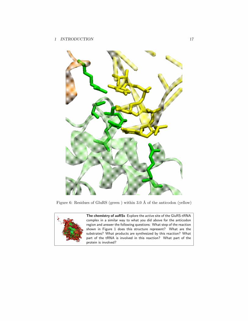


![An Aminoacyl-tRNA Synthetase Complex Escherichia coli(iii) Freezepress. Cellpellets weesuspendedin 2volumes ofbuffer Aandaddedto afreeze press (Eatonmodification oftheHughespress[7]),](https://static.documents.pub/doc/80x56/5e4dfce8f29b5d54b52a0e06/an-aminoacyl-trna-synthetase-complex-escherichia-coli-iii-freezepress-cellpellets.jpg)


