137
Class Notes for MATH 355. by S. W. Drury Copyright c 2002–2007, by S. W. Drury.
Class Notes for MATH 355.
byS. W. Drury
Copyright c© 2002–2007, by S. W. Drury.

Contents
Starred chapters and sections should be omitted on a first reading. Double starredsections should be omitted on a second reading.
1 Measuring sets on the Line 11.1 Fields and σ-fields . . . . . . . . . . . . . . . . . . . . . . . . . 31.2 Extending the notion of length — first steps . . . . . . . . . . . 81.3 Fields and σ-fields generated by a family of sets . . . . . . . . . 91.4 Extending premeasures from fields to σ-fields . . . . . . . . . . 121.5 Borel sets and Lebesgue sets . . . . . . . . . . . . . . . . . . . . 171.6 Uniqueness of the Extension . . . . . . . . . . . . . . . . . . . 201.7 Monotone Classes* . . . . . . . . . . . . . . . . . . . . . . . . 231.8 Completions of Measure Spaces . . . . . . . . . . . . . . . . . . 251.9 Approximating sets in Lebesgue measure . . . . . . . . . . . . . 281.10 A non-measurable set . . . . . . . . . . . . . . . . . . . . . . . 30
2 Integration over Measure Spaces 332.1 Measurable functions . . . . . . . . . . . . . . . . . . . . . . . 332.2 More on Measurable Functions* . . . . . . . . . . . . . . . . . 352.3 The Lebesgue Integral — first steps . . . . . . . . . . . . . . . . 362.4 The Lebesgue Integral for real and complex valued functions . . . 422.5 Interchanging limits and integrals . . . . . . . . . . . . . . . . . 442.6 Riemann and Lebesgue Integrals . . . . . . . . . . . . . . . . . 49
3 Lp spaces 513.1 Completeness of the Lp spaces . . . . . . . . . . . . . . . . . . 543.2 L2 as an inner product space . . . . . . . . . . . . . . . . . . . 583.3 Dense subsets of Lp . . . . . . . . . . . . . . . . . . . . . . . . 583.4 Duality between Lp and Lp′ . . . . . . . . . . . . . . . . . . . . 603.5 Interplay between Measure and Topology . . . . . . . . . . . . . 62
i

4 Products of Measure Spaces 704.1 The product σ-field . . . . . . . . . . . . . . . . . . . . . . . . 714.2 The Monotone Class Approach to Product Spaces* . . . . . . . . 744.3 Fubini’s Theorem . . . . . . . . . . . . . . . . . . . . . . . . . 754.4 Estimates on Homogenous kernels* . . . . . . . . . . . . . . . . 784.5 Uniqueness of Translation Invariant Measures . . . . . . . . . . 804.6 Infinite products of probability spaces** . . . . . . . . . . . . . 81
5 Hilbert Spaces 845.1 Orthogonal Projections . . . . . . . . . . . . . . . . . . . . . . 865.2 Conditional Expectation Operators . . . . . . . . . . . . . . . . 875.3 Linear Forms on Hilbert Space . . . . . . . . . . . . . . . . . . 915.4 Orthonormal Sets . . . . . . . . . . . . . . . . . . . . . . . . . 915.5 Orthonormal Bases . . . . . . . . . . . . . . . . . . . . . . . . 95
6 Convergence of Functions 99
7 Fourier Series 1027.1 Dirichlet and Fejer Kernels . . . . . . . . . . . . . . . . . . . . 1047.2 The Uniform Boundedness Principle . . . . . . . . . . . . . . . 1077.3 More about Convolution . . . . . . . . . . . . . . . . . . . . . 109
8 Differentiation 1138.1 The hardy–Littlewood Maximal Function . . . . . . . . . . . . . 1148.2 The Martingale Maximal Function on R* . . . . . . . . . . . . . 1168.3 Fundamental Theorem of Calculus . . . . . . . . . . . . . . . . 1188.4 Jacobian Determinants and Change of Variables* . . . . . . . . . 119
9 Fourier Transforms* 1249.1 Fourier Transforms of L1 functions . . . . . . . . . . . . . . . . 1279.2 Fourier Transforms of L2 functions . . . . . . . . . . . . . . . . 1289.3 Fourier Inversion . . . . . . . . . . . . . . . . . . . . . . . . . 1309.4 Defining the Fourier Transform on L1 + L2 . . . . . . . . . . . . 132
ii

1
Measuring sets on the Line
In this chapter we look at the question of how to assign a “length” to a subset of R.It’s fairly clear that this is something that might be desirable to do. The motivationcomes from the desire to define the Lebesgue Integral. The Riemann integral isdefined by making a “vertical” decomposition of the space on which the functionis defined. The advantage of doing this is that the sets of the decomposition areintervals and it is easy to decide what the length of an interval is. Lebesgue himselfmentioned the situation of someone collecting money and wanting to discoverwhat the day’s takings are. There are two ways of doing this. The first way, is tokeep a running total of the takings at each point in time. So, if at some point wereceive a quarter and then a dime, we first add 25 cents and then 5 cents. Thesecond approach is to collect all the nickels together, all the dimes together and allthe quarters together and at the end of the day find out how many of each thereare. This corresponds to a “horizontal” decomposition in defining an integral.The horizontal method turns out to have distinct advantages over the vertical,but there is one initial problem to be tackled. The horizontal decomposition of afunction will lead to sets of the form
x; y1 ≤ f(x) < y2
and we will need to decide what the length of this set is. So, we will need a theoryof length for rather general subsets of the real line.Another major impetus for developing so called measure theory is the theory
of probability. Here we have a space Ω called the sample space. A point in Ωtypically represents a particular outcome of an experiment. Usually we are notinterested in individual outcomes, but rather in sets of outcomes that satisfy somecriterion. Such a set is called an “event”. Events are assigned a probability of
1

occurring. This is like assigning a length to a subset of [0, 1]. The situation isonly slightly special in that the probability of the event of all possible outcomesΩ is necessarily equal to unity. We then talk of random variables which are func-tions defined on the sample space and their integrals with respect to the givenprobability measure defines the expectation of the random variable.Measure theory is necessarily a complicated subject because, in many situa-
tions, it turns out to be impossible to assign a sensible length to every subset. Atelling example is due to Banach and Tarski. It relates to paradoxical decomposi-tions. Let a group G act on a space X . The action is paradoxical if for positiveintegersm and n, there are disjoint subsets A1, A2, . . . , Am, B1, B2, . . . , Bn of Xand elements g1, . . . , gm, h1, . . . , hn of G such that
X =m⋃
j=1
gj · Aj
X =n⋃
k=1
hk ·Bk
The paradox is that if µ is some kind of G-invariant measure which applies to allsubsets of X , then we will be forced to have (because of the disjointness) that
µ(X) ≥m∑
j=1
µ(Aj) +n∑
k=1
µ(Bk)
and yet
µ(X) ≤m∑
j=1
µ(gj · Aj) =m∑
j=1
µ(Aj)
µ(X) ≤n∑
k=1
µ(hk ·Bk) =n∑
k=1
µ(Bk)
leading to 2µ(X) = µ(X) + µ(X) ≤m∑
j=1
µ(Aj) +n∑
k=1
µ(Bk) ≤ µ(X).
A weak form of the Banach–Tarski paradox states that the action of the rota-tion group on the sphere in Euclidean 3-space is paradoxical. One is forced toconclude that if one wants a viable theory, then it will only be possible to measurenice sets. Usually, there will be nasty sets that have pathological properties.
2

1.1 Fields and σ-fields
This means that we need to look at collections of subsets with certain properties.We will meet various types of such collections in this course. The most prevalentone will be the σ-field . Our main focus will be the real line. Before definingσ-fields we will establish the following result which will be the starting point forLebesgue measure.
THEOREM 1 Let K be a countable index set. I = [a, b[ and Ik = [ak, bk[ fork ∈ K We have
(i) If⋃
k Ik ⊆ I and the Ik are disjoint, then∑
k length(Ik) ≤ length(I).
(ii) If I ⊆⋃
k Ik, then length(I) ≤∑
k length(Ik).
(iii) If⋃
k Ik = I and the Ik are disjoint, then∑
k length(Ik) = length(I).
Proof.
(i) Let us assume that K is finite to start with. Then we can assume thatK = 1, 2, . . . , n. We will proceed by induction on n. If n = 1 thenI1 ⊆ I clearly implies that a1 ≥ a and b1 ≤ b so length(I1) = b1 − a1 ≤b− a = length(I). The induction starts.
Now let us assume that the result is true for n− 1 intervals. Let us reorderthe intervals such that ak are increasing with k. This affects neither thehypotheses nor the conclusion. Now for 1 ≤ k < n, bk ≤ an for, if notthen an ∈ Ik since certainly ak ≤ an. Thus
n−1⋃k=1
Ik ⊆ I ∩ ]−∞, an[= [a, an[.
Applying the induction hypothesis, this gives∑n−1
k=1 length(Ik) ≤ an − a.But, we also have that bn ≤ b, for if not, there is a point of In close to bnwhich is not in I . So, length(In) = bn − an ≤ b − an. It follows that∑n
k=1 length(Ik) ≤ (an − a) + (b− an) = b− a, completing the inductionstep.
To establish the result when K is infinite, it suffices to assume without lossof generality that K = N and to let n tend to infinity in the finite case.
3

(ii) Let us assume that K is finite to start with. Then we can assume thatK = 1, 2, . . . , n. We will proceed by induction on n. If n = 1 thenthe induction starts as before. Now let us assume that the result is true forn− 1 intervals. Let us reorder the intervals such that ak are increasing withk. Again, this affects neither the hypotheses nor the conclusion. First weconsider the case where a ≥ b1. Then I∩I1 = ∅ and already I ⊆
⋃nk=2 Ik so
that by the induction hypothesis (b−a) ≤∑n
k=2(bk−ak) ≤∑n
k=1(bk−ak)as required. So, we may always assume that a < b1. Now observe that
[b1, b[⊆n⋃
k=2
Ik
since if x ∈ [b1, b[, then x ∈ [a, b[⊆⋃n
k=1 Ik, but x /∈ I1. Therefore by theinduction hypothesis b − b1 ≤
∑nk=2(bk − ak). But a ≥ a1 for otherwise
a /∈⋃n
k=1 Ik. So we get
b− a = (b1 − a) + (b− b1) ≤ (b1 − a1) +n∑
k=2
(bk − ak) =n∑
k=1
(bk − ak)
as required.
Now for the case K infinite. We can assume that k = N. We want touse compactness to reduce to the case of finitely many intervals. But thiswon’t work directly, so we want to make the contained interval closed andbounded and the containing intervals open. Let ε > 0. Then we have
[a, b− ε] ⊆∞⋃
k=1
]ak − 2−kε, bk[
and by compactness, there exists an integer n such that
[a, b− ε] ⊆n⋃
k=1
]ak − 2−kε, bk[
and
[a, b− ε[⊆n⋃
k=1
[ak − 2−kε, bk[
Therefore, from the finite result, we have
b− a− ε ≤n∑
k=1
(bk − ak + 2−kε) ≤ ε+∞∑
k=1
(bk − ak)
4

Since ε is an arbitrary positive number, the result follows.
(iii) Follows immediately from (i) and (ii) above.
In Theorem 1 above, we had in mind that the endpoints of the intervals shouldbe real numbers. We can also ask what happens if we allow either I of Ik to takeeither of the forms ]−∞, b[, [a,∞[ or ]−∞,∞[.
COROLLARY 2 Let K be a countable index set. I and Ik for k ∈ K be generalintervals, closed on the left and open on the right. If
⋃k Ik = I and the Ik are
disjoint, then∑
k length(Ik) = length(I).
Proof. The only problem is when one or more of the intervals has infinite length.Obviously, if one of the Ik has infinite length, so does I and
∑k length(Ik) =
∞ = length(I). The only contentious case is when I has infinite length, but allthe Ik have finite length. In this case, let c > 0. We have by Theorem 1, (ii) thatlength(I ∩ [−c, c[) ≤
∑k∈K length(Ik). We find that length(I ∩ [−c, c[) −→ ∞
as c −→∞ and it follows that∑
k length(Ik) = ∞ as required.
We can now make progress on general measure theory.
DEFINITION Let X be a set. Then a collection F of subsets of X is a field(sometimes called an algebra) if and only if
(i) X ∈ F .
(ii) A ∈ F =⇒ X \ A ∈ F .
(iii) A ∈ F , B ∈ F =⇒ A ∪B ∈ F .
The immediate consequences of this definition are:
• ∅ ∈ F .
• Ak ∈ F for k ∈ K, K finite =⇒⋃
k∈K Ak ∈ F .
• Ak ∈ F for k ∈ K, K finite =⇒⋂
k∈K Ak ∈ F .
In the same vein we have the following definition.
5

DEFINITION Let X be a set. Then a collection F of subsets of X is a σ-field(sometimes called a σ-algebra ) if and only if
(i) X ∈ F .
(ii) A ∈ F =⇒ X \ A ∈ F .
(iii) Ak ∈ F for k ∈ K, K countable =⇒⋃
k∈K Ak ∈ F .
The immediate consequences of this definition are:
• ∅ ∈ F .
• Ak ∈ F for k ∈ K, K countable =⇒⋂
k∈K Ak ∈ F .
• F a σ-field =⇒ F a field.
DEFINITION We can now define the concept of a measure (sometimes calleda countably additive set function) on a field F of subsets of X as a functionµ : F −→ [0,∞] such that
(i) µ(∅) = 0.
(ii) µ(⋃
k∈K Ak
)=∑
k∈K µ(Ak) whenever K is a countable index set and Ak
are pairwise disjoint subsets of X with Ak ∈ F and⋃
k∈K Ak ∈ F .
Sometimes if F is a field rather than a σ-field , µ is called a premeasure ratherthan a measure.It’s worth observing explicitly that we are allowing measures to take the value
∞. We interpret sums of nonnegative series with possibly infinite terms in theobvious way. So, if just one term in the series
∑k∈K µ(Ak) is infinite, the whole
sum is infinite. If not, then the series is treated as a series of nonnegative termsand it evaluates to a real number if the series converges and to ∞ if the seriesdiverges.Now we need to look at complementation, because this will come to plague
us later. If A,B ∈ F and µ(A) = µ(B) where µ is a measure on F , then canwe deduce that µ(Ac) = µ(Bc)? We have of course µ(X) = µ(A) + µ(Ac) andµ(X) = µ(B) + µ(Bc), so with the normal laws of arithmetic we have µ(Ac) =µ(Bc). Indeed, if µ(X) <∞ this is clearly the case because the measures of all thesets involved are nonnegative real numbers. But if µ(A) = µ(B) = µ(X) = ∞then nothing whatever can be said about µ(Ac) and µ(Bc).There is another important property of measures.
6

LEMMA 3 LetF be a σ-field and suppose that µ is a measure onF . Let Fj ∈ Fbe an increasing sequence of sets, then µ
(⋃j Fj
)= supj µ(Fj).
Proof. We define A1 = F1, Aj = Fj \Fj−1 for j = 2, 3, . . .. Then Aj are disjointsubsets in F . Therefore
µ
(∞⋃
j=1
Aj
)=
∞∑j=1
µ(Aj) = µ(F1) +∞∑
j=2
(µ(Fj)− µ(Fj−1)
)= sup
jµ(Fj).
That’s a lot of definitions, so we had better have some examples.
• Let X any set and let F be the collection of all subsets of X . That will be aσ-field. For a measure we can simply let µ(A) be the number of elementsin A with the understanding that µ(A) = ∞ if A is infinite. It’s intuitivelyclear that µ is a measure on F , but that would require some proof. Thismeasure is called the counting measure because it simply counts the num-ber of elements in the set.
• Let X = N and again let F be the collection of all subsets of X . Assign aweight wn ≥ 0 to each n ∈ N. Now define
µ(A) =∑n∈A
wn
with the understanding that µ(A) = ∞ if the series diverges. The terms of aseries of positive terms can be rearranged without affecting the convergenceor the value of the sum (or we can work with unconditional sums — seethe notes for MATH 255).
• Let X = N and let F be the collection of subsets of X that are either finiteor cofinite This is a field, but not a σ-field. You can assign a premeasure toF as in the last example.
• Let X be an uncountable set and let F be the collection of subsets of Xthat are either finite or cofinite This is a field, but not a σ-field. Now, letµ(A) = 0 if A is finite and µ(A) = 1 if A is cofinite.
• Let X and F be as in the last example. Now, let µ(A) = 0 if A is finite andµ(A) = ∞ if A is cofinite.
7

• Let X = 1, 2, 3, 4, 5, 6, F the set of all subsets of X and µ(A) = |A|/6.Then µ(A) is the probability measure of a fair dice.
DEFINITION A probability measure is a measure with the additional propertythat µ(X) = 1.
It follows easily from the definitions that if µ is a probability measure then µtakes its values in the interval [0, 1].It will be noted that we are quite short on interesting examples. We work to
remedy that situation. It will also be noted that we allow a measure to be definedon a field rather than a σ-field which might seem (correctly) to be its natural baseof operations. Allowing this possibility gives us room for manœvre.
1.2 Extending the notion of length — first steps
So in this section, we will let X = R and F is the collection of all subsets of Rthat are finite unions of intervals closed on the left and open on the right. Thereis no restriction on the length of the intervals except perhaps that we can alwaysconsider it to be strictly positive for otherwise the interval would be empty. LetF ∈ F and consider C a component of F . This is a connected subset of F andtherefore also of R. So, C is an interval. Now every constituent interval of F iscontained in some component C and it follows that C is just the (finite) unionof those constituent intervals which it contains. Thus, C is closed on the left andopen on the right and it follows that distinct components are not merely disjoint,but also cannot abut. So every set F ∈ F can be written in a unique way as
F =n⋃
k=1
Ik
where Ik are intervals closed on the left and open on the right that are disjointand do not abut. It is now easy to see that the R \F is also an element of F . Thismeans that F is a field. Let us now define µ(F ) =
∑nk=1 length(Ik).
THEOREM 4 The set function µ is a premeasure on F .
Proof. Let Fj ∈ F be disjoint for j ∈ N, F ∈ F and F =⋃
j Fj . Then we haveto show that
µ(F ) =∑
j
µ(Fj).
8

We will write Fj =⋃Kj
k=1 Ij,k and F =⋃K
k=1 Jk where Ij,k and Jk are intervalsclosed on the left and open on the right. All of these unions are of the disjointvariety. We get
µ(F ) =K∑
k=1
length(Jk) (1.1)
=K∑
k=1
∞∑j=1
Kj∑`=1
length(Jk ∩ Ij,`) (1.2)
=∞∑
j=1
Kj∑`=1
K∑k=1
length(Jk ∩ Ij,`) (1.3)
=∞∑
j=1
Kj∑`=1
length(Ij,`) (1.4)
=∞∑
j=1
µ(Fj) (1.5)
Here (1.1) is the definition of µ(F ), (1.2) follows by Corollary 2 applied to Jk =⋃j,` Jk ∩ Ij,`, (1.3) follows from changing the order of summation in a series of
positive terms, (1.4) follows since Ij,` ⊆ F and by using Corollary 2 applied toIj,` =
⋃Kk=1 Jk ∩ Ij,`. Finally (1.5) follows by the definition of µ(Fj).
1.3 Fields and σ-fields generated by a family of sets
Let X be a set and A a family of subsets of X . We define the field and theσ-field generated by A by considering the collection of all fields (respectivelyσ-fields ) on X which contain the given collection A and take the intersectionof the collection. Explicitly
field generated by A =⋂
F is a fieldF⊇A
F
σ-field generated by A =⋂
F is a σ-fieldF⊇A
F
9

There are two important considerations here. The first is that the power set ofX , (i.e. the collection of all subsets of X) is a field (respectively σ-field) on X .The second is that an arbitrary intersection of fields (respectively σ-fields) is againa field (respectively σ-field). We can legitimately say that the field (respectivelyσ-field) generated byA is the smallest field (respectively σ-field) onX containingA.This definition from the outside is very unappealing. It’s really difficult to get a
handle on what it means. In the case of a field, it is possible to give a definitionfrom the inside but for the σ-field, this is unfortunately not the case. For fields wehave the following lemma.
LEMMA 5 Let X be a set and A any collection of subsets of X . Let F be thefield generated by A. Then a subset F of X lies in F if and only if the followingcondition holds:
There is an integer N ≥ 1 and a chain of sets (Fn)Nn=1 defined for
n = 1, 2, . . . , N by one of the following options:
• Fn = X .
• Fn ∈ A,• Fn = Fpn \ Fqn with 1 ≤ pn, qn < n.
• Fn = Fpn ∪ Fqn with 1 ≤ pn, qn < n.
and with F = FN .
Proof. One proves easily by induction that Fn ∈ F . In the opposite direction,let the collection of all subsets that are defined by a chain of this type by G. Thenclearly A ⊆ G. We only need to show that G is a field. We have X ∈ G. Now letG,H ∈ G. Then there are chains of sets (Gn)P
n=1 and (Hn)Qn=1 with GP = G and
HQ = H. It is now evident that one may define and new chain (Fn)P+Q+1n=1 by
• Fn = Gn if n = 1, 2, . . . , P .
• Fn = Hn−P if n = P + 1, P + 2, . . . , P +Q.
• FP+Q+1 = FP \ FP+Q(= G \ H) or FP+Q+1 = FP ∪ FP+Q(= G ∪ H)depending on case.
10

This shows that G is closed under set-theoretic difference and union and is there-fore a field.
It is the curse of measure theory that no corresponding result is true forσ-fields1. When discussing the σ-field generated by a family of sets we have to gothrough contortions.
EXAMPLE Consider for example the following question
IfM is a σ-field of subsets ofX and S is a subset ofX , show thatthe σ-field generated byM∪ S is
(A ∩ S) ∪ (B ∩ Sc);A,B ∈M.
We will prove in a moment that H = (A ∩ S) ∪ (B ∩ Sc);A,B ∈ M is aσ-field on X . On the other hand, if G is a σ-field withM ⊆ G and S ∈ G, then(A∩ S)∪ (B ∩ Sc) ∈ G whenever A,B ∈M, soH ⊆ G. It follows thatH is thesmallest σ-field containingM and S.To establish the claim, observe that X = (X ∩ S) ∪ (X ∩ Sc) ∈ H. Further
((A ∩ S) ∪ (B ∩ Sc))c = (Ac ∪ Sc) ∩ (Bc ∪ S)
= (Ac ∩Bc) ∪ (Sc ∩Bc) ∪ (Ac ∩ S) ∪ (Sc ∩ S)
= (Sc ∩Bc) ∪ (Ac ∩ S) ∈ H
since Sc ∩ S = ∅ and
Ac ∩Bc = (Sc ∩ Ac ∩Bc) ∪ (S ∩ Ac ∩Bc) ⊆ (Sc ∩Bc) ∪ (Ac ∩ S).
On the other hand, we have
∞⋃k=1
((Ak ∩ S) ∪ (Bk ∩ Sc)
)=
((∞⋃
k=1
Ak
)∩ S
)∪
((∞⋃
k=1
Bk
)∩ Sc
),
showing that H is a σ-field.2
1This is not strictly true, but you will need to understand transfinite induction in order to stateit.
11

1.4 Extending premeasures from fields to σ-fields
In this section our objective is the following result.
THEOREM 6 (CARATHEODORY’S EXTENSION THEOREM) Let µ be a premea-sure on a field F of subsets ofX . Let G be the σ-field generated by F . Then thereexists a measure ν on G which agrees with µ on F .
The first step in the proof of the Caratheodory Extension Theorem is the con-struction of an outer measure . As opposed to measures, which are defined onfields, outer measures are defined on all subsets of the ambient space X .
DEFINITION An outer measure θ on a set X is a map θ : PX −→ [0,∞] withthe following properties
(i) θ(∅) = 0.
(ii) If A ⊆ B ⊆ X , then θ(A) ≤ θ(B). We refer to this as θ being monotone .The larger the subset, the larger the value of the set function.
(iii) θ(⋃∞
j=1Aj
)≤∑∞
j=1 θ(Aj). We express this condition as θ being count-
ably subadditive .
LEMMA 7 Let µ be a premeasure on a field F of subsets ofX . Let a set functionµ? be defined on PX by
µ?(A) = inf∞∑
j=1
µ(Aj) (1.6)
where the infimum is taken over all possible sequences of sets Aj ∈ F such thatA ⊆
⋃∞j=1Aj . Then µ? is an outer measure on X .
Proof. First notice that in defining the infimum, we can always take A1 = X andAj = ∅ for j = 2, 3, . . .. Thus, there is always at least one covering over whichthe infimum is taken. Conditions (i) and (ii) in the definition of outer measure
12
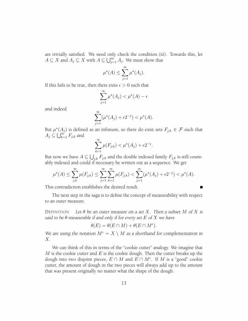
are trivially satisfied. We need only check the condition (iii). Towards this, letA ⊆ X and Aj ⊆ X with A ⊆
⋃∞j=1Aj . We must show that
µ?(A) ≤∞∑
j=1
µ?(Aj).
If this fails to be true, then there exits ε > 0 such that∞∑
j=1
µ?(Aj) < µ?(A)− ε
and indeed∞∑
j=1
(µ?(Aj) + ε2−j) < µ?(A).
But µ?(Aj) is defined as an infimum, so there do exist sets Fj,k ∈ F such thatAj ⊆
⋃∞k=1 Fj,k and
∞∑k=1
µ(Fj,k) < µ?(Aj) + ε2−j.
But now we have A ⊆⋃
j,k Fj,k and the double indexed family Fj,k is still count-ably indexed and could if necessary be written out as a sequence. We get
µ?(A) ≤∞∑j,k
µ(Fj,k) ≤∞∑
j=1
∞∑k=1
µ(Fj,k) <∞∑
j=1
(µ?(Aj) + ε2−j) < µ?(A).
This contradiction establishes the desired result.
The next step in the saga is to define the concept of measurability with respectto an outer measure.
DEFINITION Let θ be an outer measure on a set X . Then a subset M of X issaid to be θ-measurable if and only if for every set E of X we have
θ(E) = θ(E ∩M) + θ(E ∩M c).
We are using the notation M c = X \M as a shorthand for complementation inX .
We can think of this in terms of the “cookie cutter” analogy. We imagine thatM is the cookie cutter and E is the cookie dough. Then the cutter breaks up thedough into two disjoint pieces, E ∩ M and E ∩ M c. If M is a “good” cookiecutter, the amount of dough in the two pieces will always add up to the amountthat was present originally no matter what the shape of the dough.
13

PROPOSITION 8 Let θ be an outer measure on a setX . LetM be the collectionof all subsets of X that are θ-measurable. ThenM is a σ-field and the restrictionof θ toM is a measure.
We prove Proposition 8 in several steps.
Proof thatM is a field. It is immediately obvious that X ∈ M and also thatM ∈ M implies that M c ∈ M. So it remains only to establish that (iii) of thedefinition of a field holds. Towards this, it will suffice to show
A,B ∈M =⇒ A ∩B ∈M
since we already know thatM is closed under complementation. We have
θ(E) = θ(E ∩ A) + θ(E ∩ Ac).
Now apply B as a “cookie cutter” to both E ∩ A and E ∩ Ac
θ(E) = θ(E ∩ A ∩B) + θ(E ∩ A ∩Bc) + θ(E ∩ Ac ∩B) + θ(E ∩ Ac ∩Bc).
Next we use the subadditivity of θ to get
θ(E) ≥ θ(E ∩ A ∩B) + θ((E ∩ A ∩Bc) ∪ (E ∩ Ac ∩B) ∪ (E ∩ Ac ∩Bc)
),
= θ(E ∩ A ∩B) + θ(E ∩ ((A ∩Bc) ∪ (Ac ∩B) ∪ (Ac ∩Bc))),
= θ(E ∩ A ∩B) + θ(E ∩ (A ∩B)c).
Using the subadditivity again, we get
θ(E) ≤ θ(E ∩ A ∩B) + θ(E ∩ (A ∩B)c).
Combining the two inequalities gives
θ(E) = θ(E ∩ A ∩B) + θ(E ∩ (A ∩B)c)
and this completes the proof thatM is a field.
LEMMA 9 Let Aj ∈M for j ∈ J where J is a countable index set and supposethat the Aj are pairwise disjoint. Then for every E ⊆ X we have
θ
(E ∩
(⋃j∈J
Aj
))=∑j∈J
θ(E ∩ Aj). (1.7)
14

Proof. Let us first consider the case where J is finite. Let J have n elements.If n = 1, then (1.7) is a tautology. If n = 2, then since A1 ∈ M and by thedisjointness of A1 and A2,
θ(E ∩ (A1 ∪ A2)) = θ(E ∩ (A1 ∪ A2) ∩ A1) + θ(E ∩ (A1 ∪ A2) ∩ Ac1)
= θ(E ∩ A1) + θ(E ∩ A2)
For n ≥ 3 we use strong induction on n. We have
θ
(E ∩
(n⋃
k=1
Ak
))= θ(E ∩ A1) + θ
(E ∩
(n⋃
k=2
Ak
))
= θ(E ∩ A1) +n∑
k=2
θ(E ∩ Ak)
=n∑
k=1
θ(E ∩ Ak)
where the induction hypothesis has been used with 2 sets in the first line and withn− 1 sets in the second line. This completes the finite case. For the infinite case,we have
θ
(E ∩
(∞⋃
k=1
Ak
))≥ θ
(E ∩
(n⋃
k=1
Ak
))=
n∑k=1
θ(E ∩ Ak).
Letting n tend to infinity now gives
θ
(E ∩
(∞⋃
k=1
Ak
))≥
∞∑k=1
θ(E ∩ Ak).
On the other hand using the countable subadditivity of θ we have the reverseinequality
θ
(E ∩
(∞⋃
k=1
Ak
))≤
∞∑k=1
θ(E ∩ Ak)
and combining the two inequalities completes the proof of the lemma.
Completion of the proof of Proposition 8.
15
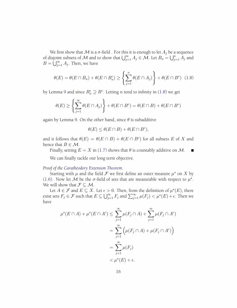
We first show thatM is a σ-field . For this it is enough to let Aj be a sequenceof disjoint subsets ofM and to show that
⋃∞j=1Aj ∈M. Let Bn =
⋃nj=1Aj and
B =⋃∞
j=1Aj . Then, we have
θ(E) = θ(E ∩Bn) + θ(E ∩Bcn) ≥
n∑
j=1
θ(E ∩ Aj)
+ θ(E ∩Bc) (1.8)
by Lemma 9 and since Bcn ⊇ Bc. Letting n tend to infinity in (1.8) we get
θ(E) ≥
∞∑
j=1
θ(E ∩ Aj)
+ θ(E ∩Bc) = θ(E ∩B) + θ(E ∩Bc)
again by Lemma 9. On the other hand, since θ is subadditive
θ(E) ≤ θ(E ∩B) + θ(E ∩Bc),
and it follows that θ(E) = θ(E ∩ B) + θ(E ∩ Bc) for all subsets E of X andhence that B ∈M.Finally, setting E = X in (1.7) shows that θ is countably additive onM.
We can finally tackle our long term objective.
Proof of the Caratheodory Extension Theorem.Starting with µ and the field F we first define an outer measure µ? on X by
(1.6). Now letM be the σ-field of sets that are measurable with respect to µ?.We will show that F ⊆M.Let A ∈ F and E ⊆ X . Let ε > 0. Then, from the definition of µ?(E), there
exist sets Fj ∈ F such that E ⊆⋃∞
j=1 Fj and∑∞
j=1 µ(Fj) < µ?(E)+ ε. Then wehave
µ?(E ∩ A) + µ?(E ∩ Ac) ≤∞∑
j=1
µ(Fj ∩ A) +∞∑
j=1
µ(Fj ∩ Ac)
=∞∑
j=1
(µ(Fj ∩ A) + µ(Fj ∩ Ac)
)
=∞∑
j=1
µ(Fj)
< µ?(E) + ε.
16

Passing to the limit as ε → 0 we get µ?(E ∩ A) + µ?(E ∩ Ac) ≤ µ?(E). Bysubadditivity we get µ?(E∩A)+µ?(E∩Ac) ≥ µ?(E) and it follows thatA ∈M.Next, we need to show that µ and µ? agree on F . Given F ∈ F , we can set
A1 = F , Aj = ∅ for j = 1, 2, . . . to get µ?(F ) ≤ µ(F ). To get the inequality inthe opposite direction, we must show that whenever Aj ∈ F and F ⊆
⋃∞j=1Aj
we necessarily have
θ(F ) ≤∞∑
j=1
µ(Aj). (1.9)
We do this in two steps by manipulating the Aj . Firstly we ensure that the Aj aredisjoint by replacing A1 with itself, A2 with A2 \A1, A3 with A3 \ (A1 ∪A2), etc.This process makes the Aj smaller, so showing that (1.9) holds with the “new”Aj implies that it holds with the “original” Aj . Secondly, we replace each Aj byAj ∩F . Again, since the process makes the Aj smaller, it is enough to show (1.9)for the “new” sets. Note that both of these processes generate subsets of F . So, itis enough to show (1.9) in case that Aj are disjoint subsets of F . But in that casewe also have F =
⋃∞j=1Aj and µ?(F ) =
∑∞j=1 µ(Aj) holds since µ is a measure
on F .Now we are done because G ⊆ M and if we define ν to be the restriction of
µ? to G, then ν is clearly a measure on G.
1.5 Borel sets and Lebesgue sets
We can now apply the rather general results of the previous section to the caseof the length premeasure on the field generated by the intervals closed on the leftand open on the right. In this case, we obtain two σ-fields G andM and theseare called the Borel σ-field of R and the Lebesgue σ-field of R respectively. Tobe explicit, the Borel σ-field of R is the smallest σ-field containing the intervalsclosed on the left and open on the right. The Lebesgue σ-field on the other handis the σ-field of all sets that are measurable with respect to the “length” outermeasure.In fact it is possible to define the Borel σ-field for any metric space X . It is
clear that every open interval in R is a countable union of intervals closed on theleft and open on the right. So every open interval is in G. On the other hand,every interval closed on the left and open on the right is a countable intersectionof open intervals. So, in fact, the open intervals and the intervals closed on the
17
left and open on the right generate the same σ-field . Also, every open subset ofR is a countable union of open intervals, so that G is also the σ-field generated bythe open sets. This prompts the following definition.
DEFINITION Let X be a metric space. Then the Borel σ-field BX of X is thesmallest σ-field containing the open subsets of X . A subset B of X is said to be aBorel subset of X (or just a Borel set if the context is clear) if B ∈ BX .
It goes without saying that Borel sets are very difficult to understand and toget a grip on. The only way in practice of showing that a set is Borel is to build itexplicitly out of countable unions and countable intersections starting from opensets. In fact there is a special terminology for this. A subset of a metric spaceX is said to be a Gδ if it is a countable intersection of open subsets. It is anFσ if it is a countable union of closed sets. It is a Gδσ if it is a countable unionof Gδ subsets and so on. The greek letters δ and σ stand for durchschnitt andsumme in this context. One might hope that after some fixed finite number ofsuch operations one would have captured all Borel subsets, but this unfortunatelyis not the case. To show that a subset is not a Borel subset, in practice, we have tofind a σ-field containing all the open sets, but which does not contain the givensubset.We can now state the following Corollary of the Caratheodory Extension The-
orem
COROLLARY 10 There is a measure ν defined on the Borel σ-field of R whichassigns to every interval its length.
Proof. We apply the Caratheodory Extension Theorem to the field F generatedby intervals closed on the left and open on the right. Let G be the σ-field generatedby F . Then G is just the Borel field of R and hence the length premeasure on Fextends to the σ-field of all Borel subsets of R.At the moment, it is not clear what difference there might be between the
Borel subsets and the Lebesgue subsets of R. It is clear that every Borel subset isLebesgue, but could the converse also be true? Well, it turns out that this is notthe case.
PROPOSITION 11 Both the Borel σ-field and the Lebesgue σ-field are transla-tion invariant. Also, Lebesgue measure is translation invariant.
18

Proof. Since the open subsets of R are translation invariant, it follows that theBorel σ-field of R is also translation invariant. The field F generated by intervalsclosed on the left and open on the right is translation invariant and also so isthe length premeasure µ. It follows that Lebesgue outer measure is translationinvariant
µ?(E + x) = µ?(E) ∀E ⊆ R, x ∈ R,
and therefore the Lebesgue σ-field is translation invariant and also the Lebesguemeasure ν which is just the restriction of µ?.
EXAMPLE The following example is rather counterintuitive. Let us takeX = Z,the set of all integers and let F be the collection of periodic subsets of Z. To beexplicit, a subset A of Z is periodic, if there exists an integer n ≥ 1 and a subset Bof 0, 1, 2, . . . , n−1 such that A = B+nZ. The smallest n for which this can bedone is called the period of A. Now it is clear that F is a field. If for example Aj
is a periodic subset with period nj for j = 1, 2, it is fairly straightforward to showthat Z \A1 is periodic with period n1 and that A1 ∪A2 can be represented in theform B + nZ for B ⊆ 0, 1, 2, . . . , n− 1 where n is the LCM of n1 and n2. For
an element A of F we can define a density µ(A) by µ(A) =|B|n. Intuitively, this
is the proportion of integers that are in the subset A. It is also possible to showthat µ is finitely-additive on F . This is true, because whenever one is dealing withonly finitely many sets of F , we can view everything on the period of the lowestcommon multiple of the periods of the given subsets. It seems reasonable that µwould also be a premeasure on F . However, let us consider the consequencesof this statement. Caratheodory’s Extension Theorem would then guarantee anextension ν of µ to the σ-field G generated by F . Now clearly 0 =
⋂∞n=1 nZ,
so 0 ∈ G. In fact, we can write Z \ 0 as a union⋃∞
k=1Ak of disjoint periodicsets Ak. We will have ν(0) = 1 −
∑∞k=1 µ(Ak). Equally well, we can realize
Z \ n as a union⋃∞
k=1(n+ Ak) and then
ν(n) = 1−∞∑
k=1
µ(n+ Ak) = 1−∞∑
k=1
µ(Ak) = ν(0),
so that ν(n) will be independent of n. Now ν(0) > 0 is not possiblebecause we can find a positive integer N such that Nν(0) > 1 and thenν(0, 1, 2, . . . , N) > 1 which is impossible. So it must be the case that ν(0) =0. But then 1 = ν(Z) = ν(
⋃n∈Zn) =
∑n∈Z ν(n) = 0. This contradiction
shows that the original µ cannot be countably additive. In fact, one can deduce
19

the existence of disjoint periodic subsets Ak with⋃∞
k=1Ak = Z but such that∑∞k=1 µ(Ak) < 1.We can understand this by means of an explicit example. Let
B1 = −1, 0, 1+ 8Z
B2 = −2, 2+ 16Z
B3 = −3, 3+ 32Z
Bk = −k, k+ 2k+2Z (k ≥ 2)
Then it is clear that⋃∞
k=1Bk = Z and∑∞
k=1 µ(Bk) = 9/16 < 1. The Bk are notdisjoint, but they can be made so following standard procedures. 2
1.6 Uniqueness of the Extension
In the previous section we proved the existence of an extension. What aboutthe uniqueness? Could there be more than one possible extension. Well underreasonable hypotheses, the answer is no. The extra condition that is needed tomake this conclusion possible is one that occurs a great deal in measure theory. Itis called σ-finiteness.
DEFINITION Let F be field or σ-field on a set X . Let µ be a measure on F .Then µ is said to be finite if and only if µ(X) <∞.
DEFINITION Let F be field or σ-field on a set X . Let µ be a measure on F .Then µ is said to be σ-finite if and only if there exists a sequence of subsets (Xj)of X with Xj ∈ F , µ(Xj) <∞ for all j and X =
⋃∞j=1Xj .
There are two approaches to the uniqueness question. We will develop themboth. The first approach is the one favoured by probabilists.
DEFINITION Let X be a set. Then a collection of subsets P of X is said to be aπ-system if
(π1) A,B ∈ P =⇒ A ∩B ∈ P .
On the other hand we also make the following definition.
20

DEFINITION Let X be a set. Then a collection of subsets L of X is said to be aλ-system if
(λ1) X ∈ L.
(λ2) A ∈ L =⇒ X \ A ∈ L.
(λ3) WheneverA1, A2, . . . are disjoint subsets ofX in L then the union⋃∞
j=1Aj
is also in L.
In fact, if (λ1) and (λ3) are true, then (λ2) implies the condition that A,B ∈P , A ⊇ B =⇒ A \B ∈ P . This is because (A \B)c = (X \A)∪B and (X \A)and B are disjoint.The following Lemma is now fairly clear
LEMMA 12 A collection of subsets F of X which is both a π-system and aλ-system is also a σ-field .
Proof. First of all ∅ = X \ X ∈ F . Since F is closed under finite intersectionsand complementation, it is clear that it is also closed under finite unions. There-fore F is a field. But now, given a sequence A1, A2, . . . of subsets of X in F , wecan adjust them to make them disjoint, using the standard trick. We define
B1 = A1, B2 = A2 \ A1, B3 = A3 \ (A1 ∪ A2), . . .
We also have⋃∞
j=1Aj =⋃∞
j=1Bj ∈ F . Thus F is a σ-field as required.
The key result in this section is the following.
THEOREM 13 (DYNKIN’S π − λ THEOREM) If P is a π-system and L is a λ-system and P ⊆ L, then σ(P) ⊆ L where σ(P) is the σ-field generated by P .
We will need the following lemma.
LEMMA 14 Let F be a λ-system onX and suppose that A ∈ F . We define FA
the system of all subsets B ofX such that A∩B ∈ F . Then FA is also a λ-systemon X .
21
Proof. There are three axioms to check. Since X ∩ A = A ∈ F , X ∈ FA. IfB ∈ FA, then A ∩ B ∈ F and so A \ B = A \ (A ∩ B) ∈ F since F preservescontained differences. But (X \ B) ∩ A = A \ B, so X \ B ∈ FA. This showsthat FA is closed under complementation. Finally, let Bj be a disjoint sequencein FA. Then the intersections A∩Bj are also disjoint and lie in F . It follows thatA ∩
⋃∞j=1Bj =
⋃∞j=1(A ∩ Bj) ∈ F . So,
⋃∞j=1Bj ∈ FA. This shows that FA is
closed under disjoint countable unions.
Proof of Dynkin’s π − λ Theorem. Let F be the λ-system generated by P . Inother words, F is the intersection of all λ-systems containing P . It is clear thatF ⊆ L. If we can show that F is also a π-system, then it will be a σ-field and thedesired conclusion will follow.Now, let A ∈ P and B ∈ P . Then A ∩ B ∈ P ⊆ F so that B ∈ FA. By
Lemma 14, FA is a λ-system containing P . It now follows that F ⊆ FA becauseF is the intersection of all λ-systems containing P . But, this means that A ∈ Pand B ∈ F implies that A ∩ B ∈ F . So, if B ∈ F then P ⊆ FB. But then,F ⊆ FB, because again by Lemma 14 FB is a λ-system containing P and F isthe smallest such animal. So, finally we have shown that
A,B ∈ F =⇒ A ∩B ∈ F .
In other words, F is a π-system and the proof is complete.
We can now use this result to obtain information about the uniqueness ofextensions.
PROPOSITION 15 Let P be a π-system and µ1 and µ2 be finite measures onσ(P) which agree on P and on X (i.e. µ1(X) = µ2(X)). Then µ1 and µ2 agreeon σ(P).
Proof. Let L be the collection of subsets in σ(P) on which µ1 and µ2 agree. Wewill show that L is a λ-system. By hypothesis, X ∈ L. Now suppose that A ∈ L.Then µ1(A) = µ2(A). We find that µj(X \ A) + µj(A) = µj(X) for j = 1, 2.It follows that µ1(X \ A) = µ2(X \ A). It’s very important here that µj(X) isfinite. If both the µj(X) and the µj(A) are infinite, we cannot deduce the value ofµj(X \A). This shows that L satisfies both (λ1) and (λ2). The fact that it satisfies(λ3) uses the fact that µj are measures. If Aj are disjoint subsets in L, then wehave
µ1
(∞⋃
j=1
Aj
)=
∞∑j=1
µ1(Aj) =∞∑
j=1
µ2(Aj) = µ2
(∞⋃
j=1
Aj
)
22

and it follows that⋃∞
j=1Aj ∈ L. This completes the verification that L is a λ-system. Finally, Dynkin’s π-λ Theorem shows that σ(P) ⊆ L and the proof iscomplete.
The usual application is to the uniqueness of the extension in Caratheodory’sExtension Theorem.
THEOREM 16 Let µ be a σ-finite premeasure on a field F of subsets of X . LetG be the σ-field generated by F . Then there exists a unique measure ν on Gwhich agrees with µ on F .
Proof. The existence of ν is already contained in Caratheodory’s Extension The-orem. It is the uniqueness with which we are really concerned here. So, let ν1 andν2 be two possible extensions. Now, since µ is σ-finite, we can find a sequence ofsubsets (Xj) of X in F , such that µ(Xj) is finite and X =
⋃∞j=1Xj . So let Fj be
the field of those sets of F that are contained insideXj . We view this as a field onXj . Note that this field is exactly the same as the field of traces F ∩Xj;F ∈ F.Let Gj = σ(Fj). Since ν1 and ν2 agree on Fj , by Proposition 15, they also agreeon Gj . We now construct a new σ-field Hj = H;H ⊆ X, H ∩Xj ∈ Gj whichclearly contains F . Therefore, by definition of G we have G ⊆ Hj . So G ∈ Gimplies that for each j, G ∩ Xj ∈ Gj . Now, without loss of generality, we canarrange that the Xj are disjoint. So G =
⋃∞j=1G ∩Xj is a disjoint union and
ν1(G) =∞∑
j=1
ν1(G ∩Xj) =∞∑
j=1
ν2(G ∩Xj) = ν2(G).
Thus ν1 and ν2 agree on G.
1.7 Monotone Classes*
The second approach to the uniqueness problem is the one that is usually adoptedby mathematicians (as distinct from probabilists). It uses a new construct, that ofa monotone class .
DEFINITION Let X be a set. Then a collection of subsetsM of X is said to bea monotone class if
(i) Whenever A1, A2, . . . are increasing subsets of X in M then the union⋃∞j=1Aj is also inM.
23

(ii) Whenever A1, A2, . . . are decreasing subsets of X inM then the intersec-tion
⋂∞j=1Aj is also inM.
THEOREM 17 (MONOTONE CLASS THEOREM) Let F be a field. If M is amonotone class and F ⊆M, then σ(F) ⊆M.
Proof. Let M be the smallest monotone class containing F . It will suffice toshow that σ(F) = M. Note that every σ-field is a monotone class, so we haveσ(F) ⊇M. We will show thatM is in fact a σ-field . We define
MP = Q;P \Q ∈M, Q \ P ∈M, P ∪Q ∈M.It is easy to check that
• MP is a monotone class.
• P ∈MQ ⇐⇒ Q ∈MP .
Now, let P ∈ F be temporarily frozen. Then, sinceF is a field,Q ∈ F impliesthat Q ∈ MP , i.e. F ⊆ MP . ThereforeM ⊆ MP , becauseM is the smallestmonotone class containing F . So, in fact, Q ∈M implies that Q ∈MP and thisin turn implies that P ∈ MQ. So, unfreezing P and freezing Q temporarily, wehave F ⊆ MQ whenever Q ∈ M. Again becauseM is the smallest monotoneclass containing F this givesM ⊆ MQ for all Q ∈ M. But this just says thatM is closed under finite unions and set theoretic differences. So, in factM is aσ-field and the reverse inclusion σ(F) ⊆M follows.
To illustrate the application of monotone classes, let us give a second proofof Theorem 16 at least in the case where µ is a finite premeasure. The extensionto the σ-finite case follows the same ideas that are found in the first proof ofTheorem 16.It is only the uniqueness of the extension that is at issue. So, let ν1 and ν2 be
two possible extensions to σ(F). We consider
M = M ;M ∈ σ(F), ν1(M) = ν2(M).It is easy see thatM is a monotone class. For example in case Mj ∈ M andMj ↑M ∈ σ(F) we have
ν1(M) = supjν1(Mj) = sup
jν2(Mj) = ν2(M).
For decreasing sequences of sets we use complementation together with the con-dition µ(X) <∞.
24

1.8 Completions of Measure Spaces
In this section we look at a way of extending abstract measure spaces. So, let Xbe a set, G a σ-field on X and µ a measure on G. We say that a subset N of Gis a null set if µ(N) = 0. If there is a possibility of confusion between severaldifferent measures we use the terminology µ-null. Now it seems intuitively clearthat if the measure of a subset N is zero, then the measure of any subset Z of Nshould also be zero. This is very clear for instance in the case where µ is supposedto give the “length” of a subset of R. But there is a snag. The subset Z may notlie in G even if N ∈ G so that µ(Z) may not even be defined. For this reason, weintroduce the notion of completion of a measure space.
DEFINITION We define a family of sets G as follows. We say that H ∈ G iffthere exist G,N ∈ G and Z ⊆ N with N µ-null such that H = G4Z. Here wehave used 4 to denote symmetric difference G4Z = (G \ Z) ∪ (Z \ G). Wealso define a quantity µ(H) = µ(G). Then (X, G, µ) will eventually define thecompletion of (X, G, µ).
Note that symmetric differences satisfy the identity A4(A4B) = B, so wecan equally well define G by the relation H4G ⊆ N . Yet another way of describ-
ing G comes from writingH = (G \N)∪((N \Z)∪ (Z \G)
)where G \N ∈ G
and (N \ Z) ∪ (Z \ G) ⊆ N . This means that the completion G can be definedwith the union operation rather than the symmetric difference. Conceptually, thismay be a little easier. We have the following Theorem.
THEOREM 18 Let G be a σ-field on X and µ a measure on G. Then
(i) G is a σ-field .
(ii) For H ∈ G, µ(H) is well-defined.
(iii) µ is a measure on G extending µ.
Proof. We have X = X4∅ and ∅ is a null set, so X ∈ G. Now let H ∈ G.Then H = G4Z where G,N ∈ G, N is null and Z ⊆ N . But Hc = Gc4Z andGc ∈ G, soHc ∈ G. Now letHj ∈ G for j ∈ N. Then we can writeHj = Gj ∪Zj
where Gj, Nj ∈ G, Nj is null and Zj ⊆ Nj . We now have
∞⋃j=1
Hj =
(∞⋃
j=1
Gj
)∪
(∞⋃
j=1
Zj
)(1.10)
25
where⋃∞
j=1Gj ∈ G and⋃∞
j=1 Zj ⊆⋃∞
j=1Nj and⋃∞
j=1Nj is a null set in G.Hence
⋃∞j=1Hj ∈ G. The proof of (i) is complete.
Next we show that µ is well-defined. Let H4Gj ⊆ Nj for j = 1, 2. Thenwe have G14G2 = (H4G1)4(H4G2) ⊆ N1 ∪ N2. Thus µ(G14G2) = 0.Then G1 ⊆ G2 ∪ (G14G2) and it follows that µ(G1) ≤ µ(G2) and the reverseinequality holds by symmetry. So µ(G1) = µ(G2).The uniqueness just proved shows that µ extends µ. Hence also µ(∅) =
µ(∅) = 0. If the Hj in (1.10) are disjoint, then so are the Gj and it followsimmediately that
µ
(∞⋃
j=1
Hj
)= µ
(∞⋃
j=1
Gj
)=
∞∑j=1
µ(Gj) =∞∑
j=1
µ(Hj)
Finally we have
DEFINITION A measure space (X,G, µ) is complete if it is its own completion.
and also the following proposition.
PROPOSITION 19 Let θ be an outer measure on a setX . LetM be the σ-field ofθ-measurable subsets and let µ be the restriction of θ toM. Then we know fromProposition 8 that µ is a measure onM. We have
(i) If Z ⊆ X and θ(Z) = 0, then Z ∈M.
(ii) If A,Z ⊆ X and θ(Z) = 0, then θ(A) = θ(A ∪ Z).
(iii) If A,B ⊆ X and θ(A4B) = 0 then θ(A) = θ(B).
(iv) The measure space (X,M, µ) is complete.
Proof. For (i), we have θ(E) ≤ θ(E ∩ Z) + θ(E ∩ Zc) = θ(E ∩ Zc) ≤ θ(E).The first inequality comes from the subadditivity of θ and the second from themonotonicity. Hence by definition of M, Z ∈ M. For (ii) we simply haveθ(A) ≤ θ(A ∪ Z) ≤ θ(A) + θ(Z) = θ(A), where the left-hand inequality isfrom the monotonicity of θ and the right-hand one is from the subadditivity. For(iii) we simply apply (ii) twice to get θ(A) = θ(A ∪ B) = θ(B). We have used
26

the relation (A ∪ B) \ A ⊆ A4B and the monotonicity of θ, to deduce thatθ((A ∪B) \ A) = 0.Finally, for (iv), let G ∈ M and suppose that θ(G4H) = 0. Then for any
subset E of X we have (E ∩ G)4(E ∩ H) ⊆ G4H and it follows that θ((E ∩G)4(E ∩H)) = 0. Therefore θ(E ∩G) = θ(E ∩H) by (iii). Similarly we haveθ(E ∩ Gc) = θ(E ∩ Hc). Since θ(E) = θ(E ∩ G) + θ(E ∩ Gc), it now followsthat θ(E) = θ(E ∩H) + θ(E ∩Hc). Since E is an arbitrary subset of X we seethat H ∈M. That completes the proof of (iv).
COROLLARY 20 The Lebesgue σ-field L on R is complete.
Proposition 19 allows us to reconcile the approach that we have taken to mea-sure theory in these notes and an approach that used to be used many years agobut has fallen out of favour as being unnecessarily complicated. To illustrate, letµ be a measure on a σ-field F of subsets of X and suppose that µ(X) < ∞. Wenow define as before the outer measure µ?
µ?(A) = inf∞∑
j=1
µ(Aj)
where the infimum is taken over all possible sequences of sets Aj ∈ F such thatA ⊆
⋃∞j=1Aj . We can also define an inner measure µ? by
µ?(A) = µ(X)− µ?(X \ A).
We don’t say here precisely what an inner measure is, we leave that to yourimagination. We will denote by ν the restriction of µ? toM. We know that ν is ameasure onM.Let A be an arbitrary subset of X . It is easy to see, from the definition of
the infimum that given ε > 0 there exists a set B ∈ M such that A ⊆ B andν(B) ≤ µ?(A) + ε. Here in fact the set B is just a set
⋃∞j=1Aj taken from the
situation defining the infimum. Now taking a sequence of εk decreasing to zero,we get A ⊆ Bk and ν(Bk) ≤ µ?(A) + εk, and taking B =
⋂∞k=1Bk, we find
B ∈ M, A ⊆ B and µ?(A) = ν(B). In some sense, this justifies the term outermeasure, because we have found a measurable subset B of X containing A withits measure equal to the outer measure of A.Now repeat all this argument on X \ A. We will come up with a subset C
inM with C ⊆ A and ν(C) = µ?(A). Now if A ∈ M then we can apply the“cookie cutter” to the whole space
µ?(A) + µ?(X \ A) = µ?(X ∩ A) + µ?(X ∩ Ac) = µ?(X) = µ(X) <∞
27

and evidently µ?(A) = µ?(A). It is the converse statement in which we areinterested. If µ?(A) = µ?(A) then in fact
ν(C) = µ?(A) = µ?(A) = ν(B)
and since we are working in a finite measure space, ν(B \C) = 0. It now followsfrom Proposition 19 and the completeness ofM that A \C is inM and hence Ais inM. So, the µ?-measurable sets are precisely those for which the inner andouter measures coincide.
1.9 Approximating sets in Lebesgue measure
In this section, we come back to the specific topic of Lebesgue measure. We have aconcept of Lebesgue measurable set which is really very hard to grasp. So we needa way of knowing that a Lebesgue measurable set is not too bad. The way that wedo this is to show that it can be approximated by nice sets. The approximation iscarried out in terms of sets of small measure. Later on in these notes, we will lookat this same topic in a more general light.
THEOREM 21 Let E ∈ L and let ε > 0.
(i) Then there exists U open in R such that U ⊇ E and ν(U \ E) < ε.
(ii) Then there exists C closed in R such that C ⊆ E and ν(E \ C) < ε.
Proof. Let us assume to start with that E is bounded. Now by definition
ν(E) = µ?(E) = inf∞∑
j=1
µ(Fj);E ⊆∞⋃
j=1
Fj, Fj ∈ F.
Now, each Fj is a finite union of intervals closed on the left and open on the right.We might as well assume that in fact each Fj is a single such interval. So, givenε > 0, we have such intervals Fj with
∞∑j=1
µ(Fj) < ν(E) + ε/2
28

If Fj = [aj, bj[, we define Uj =]aj − 2−j−1ε, bj[ a slightly larger open interval.Then clearly E ⊆
⋃∞j=1 Uj and
∑∞j=1 µ(Uj) < ν(E) + ε. So now U =
⋃∞j=1 Uj
is open and it is clear that ν(U) ≤∑∞
j=1 µ(Uj) < ν(E) + ε. Finally, and this is akey point, since E is bounded, ν(E) <∞ and we can deduce that ν(U \E) < ε.In the case that E is unbounded, for each k ∈ N, we find an open set Vk ⊇
E ∩ [−k, k] such that ν(Vk \ (E ∩ [−k, k])) < 2−k−1ε. Let V =⋃∞
k=1 Vk. ThenV is again an open subset of R and
ν(V \E) = ν
(⋃k
(Vk \ E)
)≤∑
k
ν(Vk \E) ≤∑
k
ν(Vk \ (E ∩ [−k, k])
)< ε
Furthermore, if x ∈ E, then find k ∈ N such that |x| ≤ k, so x ∈ E ∩ [−k, k] ⊆Vk ⊆ V . That is E ⊆ V . This completes the proof of (i).To prove (ii) we simply apply (i) to R \ E.
As a corollary, we can establish the so called regularity of Lebesgue measure.For reasons that may eventually become clear, we approximate from the insidewith compact subsets of R rather than closed subsets.
COROLLARY 22 Let E ∈ L.
(i) ν(E) = infν(U);U open ⊇ E.
(ii) ν(E) = supν(K);K compact ⊆ E.
Proof. (i) is an immediate consequence of Theorem 21. Also it is clear thatν(E) = supν(K);K closed ⊆ E. So, all that really needs to be shown hereis that if C is closed, then we have ν(C) = supν(K);K compact ⊆ C. Tosee this, we set Kn = C ∩ [−n, n]. Then Kn is closed (intersection of two closedsets) and bounded and hence, by the Heine–Borel Theorem, it is compact. Butν(C) = supn ν(Kn), since Kn are increasing and have union C.
Another corollary can now be established. The proof is an exercise.
COROLLARY 23 The completion of the Borel σ-field BR on the real line withrespect to the (restriction of) Lebesgue measure is the Lebesgue σ-field .
29

1.10 A non-measurable set
Here is the simplest way of constructing a non-measurable subset of R. Considerthe cosets a+ Q of the rational numbers in R. Each such coset meets the interval[0, 1]. This is simply because for every real number a, the interval [−a, 1 − a]meetsQ. So, from each coset a+Q pick an element x(a) ∈ [0, 1] and let E be thetotality of all such elements. The key observation is that if q1 and q2 are distinctrational numbers, then q1 + E and q2 + E are disjoint sets. To see why, supposethat q1 + x(a1) = q2 + x(a2). Then Q + x(a1) = Q + x(a2) and so x(a1) andx(a2) lie in the same coset of Q in R. But we chose just one element from eachcoset, so it must be that x(a1) = x(a2) and therefore q1 = q2, contradicting thefact that q1 6= q2. Now if ν(E) > 0 we can get a contradiction as follows. Weclearly have ⋃
q∈Q∩[0,1]
(q + E) ⊆ [0, 2]
and the sets in the union are disjoint. Each has the same measure as E becauseν is translation invariant. Since there are infinitely many points in Q ∩ [0, 1], wehave a contradiction. We are forced to conclude that ν(E) = 0. But this is nogood either, because
R =⋃q∈Q
(q + E) (1.11)
effectively forcing R to have zero measure. This contradiction forces us to con-clude that E /∈ L. With a little bit more effort we can show the following.
PROPOSITION 24 Let A ⊆ R be a measurable subset of R with ν(A) > 0.Then there exists B ⊆ A with B non-measurable.
Proof. Suppose not. We will demonstrate a contradiction. So, A is a set ofpositive measure, every subset of which is measurable. Now, we have A =⋃
n∈Z([n, n+1]∩A). Choose one of the subsets [n, n+1]∩A which has positivemeasure — they cannot all have zero measure. Then it will suffice to work with[n, n + 1] ∩ A replacing A. So, after translating we can assume without loss ofgenerality that A ⊆ [0, 1].Now, with E as above, letAq = A∩(q+E) for q ∈ Q a fixed rational number.
By hypothesis, Aq is measurable. We now have⋃r∈Q∩[0,1]
(r + Aq) ⊆ [0, 2]
30

and once again, the r +Aq are disjoint as r varies over Q ∩ [0, 1]. This is becauser+Aq ⊆ (r+q)+E. Since the sets r+Aq all have the same measure, we concludeas above that ν(Aq) = 0. But now, unfreezing q ∈ Q, we have A =
⋃q∈QAq,
by (1.11). It follows that ν(A) = 0 contradicting the fact that A has positivemeasure.
COROLLARY 25 There is a subset of R which is Lebesgue measurable but notBorel.
Proof. We will prove this using the Cantor set. We will in fact use two Cantorsets K1 and K2. The first of these is the regular Cantor Ternary set based on[−1, 1]. We can write
K1 = 2
3
∞∑k=0
ωk3−k;ωk ∈ −1, 1, k = 0, 1, 2, . . ..
The second Cantor set will be constructed with a variable ratio of dissection. Atthe first step, the interval [−1, 1] is split into two closed subintervals, [−1, 1−2r0]and [2r0−1, 1]. So the right-hand interval is centred at r0 and has length 2(1−r0).We then repeat the decomposition with a different scale based on r1. so, theextreme right-hand interval at the second step is [r0 + (1 − r0)(2r1 − 1), 1] etc.The points of K2 have the form
ω0r0 + ω1(1− r0)r1 + ω2(1− r0)(1− r1)r2 + · · ·
Now, after removing the first k + 1 groups of intervals, the total length of the
set remaining is 2k∏
j=0
(2(1− rj)
). If we choose for example rj = 1/2 + 2−2−j ,
then 2∞∏
j=0
(2(1− rj)
)> 0. So we can arrange that K2 has positive measure. On
the other hand, K1 which is built with rj = 2/3 for all j = 0, 1, 2, . . ., has zeromeasure. Nevertheless, the two sets can be put into one-to-one correspondenceusing the omegas and the mappings involved are continuous in both directions.Let us denote this correspondence α : K2 −→ K1.If you believe all this, then we are practically done. Since K2 has positive
Lebesgue measure, it must contain a subset E which is not Lebesgue measurable.
31

If E is not Lebesgue measurable, then it is certainly not Borel. But now con-sider α(E) which is a subset of K1. Since α is continuous in both directions,it preserves open subsets and hence also Borel subsets. Being a Borel subset is atopological property! We conclude that α(E) is not Borel. But K1 is a closed setof zero Lebesgue measure and therefore every subset of K1 for example α(E) isnecessarily Lebesgue measurable.
32

2
Integration over Measure Spaces
2.1 Measurable functions
So, in this section we have a σ-field F of subsets of X and a measure µ on F .The first task is to integrate nonnegative simple functions. We need the conceptof measurability .
DEFINITION
(i) Let f : X −→ Y where Y is a metric space. Then f is measurable (as amapping from (X,F) to (Y, dY )) iff f−1(U) ∈ F for every open subset Uof Y .
(ii) Let f : X −→ Y where (Y,G) is a measurable space (this just means thatG is a σ-field on Y ). Then f is measurable (as a mapping from (X,F) to(Y,G)) iff f−1(G) ∈ F for every subset G ∈ G.
It is easy to prove that if f is measurable as a mapping from (X,F) to (Y, dY ),then f is measurable as a mapping from (X,F) to (Y,BY ), where BY denotes theBorel σ-field of Y . So, we can if we wish interpret (i) above as a special case of(ii). Another special case of the above situation is when both X and Y are metricspaces. Then we understand the statement that f : X −→ Y is a Borel function asthe statement that f is measurable with respect to the measurable spaces (X,BX)and (Y,BY ).We need some results that will allow us to build combinations of measurable
functions.
33

PROPOSITION 26 Let (X,F) be a measurable space and let Y1, Y2 be separablemetric spaces. Let fj : X −→ Yj be F-measurable functions for j = 1, 2. Definea new function f : X −→ Y1 × Y2 by
f(x) = (f1(x), f2(x)).
Then f is also F-measurable.
Proof. We take the product metric on Y1×Y2. Let U be an open subset of Y1×Y2.Then, according to Theorem 29 in the notes for MATH 354, U can be written asa countable union of open balls. But, in the product metric, open balls are justproducts of open balls, so we may write
U =∞⋃
j=1
(UY1(y1,j, tj)× UY2(y2,j, tj)
)and it follows that
f−1(U) =∞⋃
j=1
(f−1
1 (UY1(y1,j, tj)) ∩ f−12 (UY2(y2,j, tj))
)which is clearly in F because both f1 and f2 are measurable.
COROLLARY 27 Let (X,F) be a measurable space and let Y1, Y2 be separablemetric spaces. Let fj : X −→ Yj be F-measurable functions for j = 1, 2. Let Ybe a metric space and suppose that α : Y1× Y2 −→ Y is a borel mapping. Definea new function g : X −→ Y by
g(x) = α(f1(x), f2(x)).
Then g is also measurable. In particular, sums and products of measurable real-valued functions are measurable.
LEMMA 28 The σ-field generated by the sets ]a,∞[ as a runs through R is theBorel field BR of R.
34

Proof. Let C denote the σ-field generated by the sets ]a,∞[. We clearly have]a,∞[c=] −∞, a], so for every b ∈ R we have ] −∞, b] ∈ C. Now we can alsowrite
]−∞, b[=∞⋃
n=1
]−∞, b− 2−n]
so, ]−∞, b[∈ C for every b ∈ R. It now follows that every bounded open interval]a, b[=]a,∞[∩]−∞, b[∈ C. Thus, in fact all open intervals, bounded or not are inC and hence, all open sets. Therefore C contains all borel sets. Obviously C ⊆ BR,so the two σ-fields are equal.
COROLLARY 29 Suppose that for each n ∈ N, fn is a measurable real-valuedmapping. Then so is f = sup∞n=1 fn.
Proof. We first observe thatx;
(∞
supn=1
fn(x)
)> a
=
∞⋃n=1
x; fn(x) > a.
This means that the set on the left is measurable for every a ∈ R. But, it is clearthat σ (f−1(A)) = f−1(B);B ∈ σ(A). We apply this with f = sup∞n=1 fn andA the collection of intervals of the form ]a,∞[. It tells that f−1(B) is measurablefor every Borel subset B of R.
Obviously, the same argument also works for infima. So it will also follow thatlim sup fn = infm sup∞n=m fn is a measurable function if all of the fn are. Thesame result also holds for liminfs. This means in particular, that a pointwise limitof measurable functions is measurable.
2.2 More on Measurable Functions*
We can extend this result to a more general context with the following lemma.
LEMMA 30 Let Z be a separable metric space, and U a nonempty open subsetof Z. Then there is a sequence (zk)
∞k=1 of points of Z and δk > 0 such that
∞⋃k=1
B(zk, δk) ⊆ U ⊆∞⋃
k=1
U(zk, δk) (2.1)
where we have denoted B(z, δ) = w ∈ Z; d(z, w) ≤ δ and U(z, δ) = w ∈Z; d(z, w) < δ. In fact, the inclusions in (2.1) are equalities.
35

THEOREM 31 Let Z be a separable metric space and (X,M) a measurablespace. Let fn : X −→ Z beM-measurable functions and let fn −→
n→∞f pointwise
where f : X −→ Z. Then f isM-measurable.
Proof. We claim that for every z ∈ Z and every δ > 0, there exists a setM ∈Msuch that
f−1(U(z, δ)) ⊆M ⊆ f−1(B(z, δ)). (2.2)
To do this, we simply setM =∞⋂
m=1
∞⋃n=m
x; d(fn(x), z) < δ. This is the set of all
x such that d(fn(x), z) < δ holds for infinitely many n. With this formulation,and using the pointwise convergence of fn to f we have that (2.2) holds. (We
could equally well have takenM =∞⋃
m=1
∞⋂n=m
x; d(fn(x), z) < δ which is the set
of all x such that d(fn(x), z) < δ holds for all sufficiently large n i.e. eventually).With the claim proved, we now apply Lemma 30. For each k we can find
Mk ∈M such that
f−1(U(zk, δk)) ⊆Mk ⊆ f−1(B(zk, δk)).
and now we have for any nonempty open U in Z
f−1(U) ⊆∞⋃
k=1
f−1(U(zk, δk)) ⊆∞⋃
k=1
Mk ⊆∞⋃
k=1
f−1(B(zk, δk)) ⊆ f−1(U)
so that f−1(U) =⋃∞
k=1Mk ∈M.
2.3 The Lebesgue Integral — first steps
A measurable simple function f : X −→ [0,∞] is a function between the abovespaces which is measurable and takes only finitely many values s1, . . . , sn. Weset Aj = f−1(sj). These are disjoint sets and their union is X . We can thensuccinctly write
f =n∑
j=1
sj11Aj
36

This will be called the regimented form — the sj are all distinct, the Aj aredisjoint, measurable and nonempty and their union is the whole of X . The keypoint here is that the regimented decomposition of f is uniquely determined byf . We now define ∫
fdµ =n∑
j=1
sjµ(Aj).
We use here standard conventions with regard to arithmetic involving ∞. Ourconvention is that 0 · ∞ = ∞ · 0 = 0. So, the integral of a function that isidentically zero on a set of infinite measure is zero. The integral of ∞ times theindicator function of a null set is also zero.Now we need to know that the integral has the right properties.
PROPOSITION 32
(i) If f, g are nonnegative measurable simple functions and if f ≤ g pointwise,then
∫fdµ ≤
∫gdµ.
(ii) If fn, f are nonnegative measurable simple functions and if fn ↑ f point-wise, then
∫fndµ ↑
∫fdµ.
(iii) If f, g are nonnegative measurable simple functions and a, b ∈ [0,∞], then∫(af + bg)dµ = a
∫fdµ+ b
∫gdµ
We will need the following technical lemma.
LEMMA 33 Let f =∑m
k=1 tk11Bkwhere Bk are disjoint measurable sets, then∫
fdµ =∑m
k=1 tkµ(Bk).
Proof. Note that we have not required that the union of the Bk is X . Also someof the Bk may be empty and the numbers tk may not be distinct. Whenever a Bk
is empty, we omit that value of k and renumber the remaining Bk. If the unionof the Bk is not X , we include a new Bm+1 = X \
⋃mk=1Bk, set tm+1 = 0 and
replace m by m + 1. Neither of these operations affects the truth of the Lemma.Recall that 0 · ∞ = 0, so that even if a newly created B has infinite measure, thelemma remains unaffected.
37

Thus we may assume that Bk are nonempty and disjoint for k = 1, . . . ,mand that their union is X . On Bk, the function f takes the value tk which musttherefore be one of the sj . So, we have a map α : 1, 2, . . . ,m −→ 1, 2, . . . , nsuch that tk = sα(k). The set where f takes the value sj is then Aj and also⋃
α(k)=j Bk, so these sets must be equal.∫fdµ =
n∑j=1
sjµ(Aj) =n∑
j=1
sj
∑α(k)=j
µ(Bk) =n∑
j=1
∑α(k)=j
tkµ(Bk) =m∑
k=1
tkµ(Bk)
This completes the proof.
Proof of Proposition 32. Let us write f =∑n
j=1 sj11Aj, g =
∑mk=1 tk11Bk
both inregimented form. We can write now 11Aj
=∑m
k=1 11Aj∩Bkand therefore, we can
write
f =n∑
j=1
sj11Aj=
n∑j=1
sj
m∑k=1
11Aj∩Bk=
n∑j=1
m∑k=1
sj11Aj∩Bk
The Aj ∩ Bk are disjoint subsets, but possibly empty. We can write in the sameway
g =m∑
k=1
tk11Bk=
m∑k=1
tk
n∑j=1
11Aj∩Bk=
n∑j=1
m∑k=1
tk1Aj∩Bk
So, according to Lemma 33∫fdµ =
n∑j=1
m∑k=1
sjµ(Aj ∩Bk),
∫gdµ =
n∑j=1
m∑k=1
tkµ(Aj ∩Bk) (2.3)
Now, for each pair (j, k) there are two cases. Either Aj ∩ Bk = ∅ in which caseµ(Aj ∩ Bk) = 0 or, there exists x ∈ Aj ∩ Bk. In the second case sj = f(x) ≤g(x) = tk. So, it follows from (2.3) that
∫fdµ ≤
∫gdµ by comparing the
expansions term by term. This completes the proof of (i).Next we turn to (iii), which we prove in the same manner. We find
af + bg =n∑
j=1
m∑k=1
(asj + btk)1Aj∩Bk
so that∫(af + bg)dµ =
n∑j=1
m∑k=1
(asj + btk)µ(Aj ∩Bk) = a
∫fdµ+ b
∫gdµ
38

from (2.3) and manipulative algebra. That completes the proof of (iii).Now (ii) is much harder and we first tackle the special case f = t11B, where
t ∈ [0,∞] and B is a measurable set. We are supposing that fn are nonnegativemeasurable simple functions and that fn ↑ t11B pointwise. If t = 0, then fn ≡ 0for all n and the result is obvious. We can assume therefore that t > 0. Now, let0 < r < t and think of r as being close to t. Let Bn = x; fn(x) > r. ThenBn increases with n because the fn are increasing. Also Bn ⊆ B for otherwisefind x ∈ Bn \ B and we have 0 = t11B(x) ≥ fn(x) > r > 0. Now for eachx ∈ B, eventually we will have fn(x) > r for otherwise supn fn(x) ≤ r < t =supn fn(x). In other words
⋃nBn = B, and it follows that supn µ(Bn) = µ(B).
Since fn ≤ t11B, it follows from (i) that∫fndµ ≤ tµ(B) and therefore that
supn
∫fndµ ≤ tµ(B). This is the “easy” inequality. To get the “hard” one, we
observe that∫fndµ ≥ rµ(Bn) since f > r11Bn and on taking sups we find
supn
∫fndµ ≥ r supµ(Bn) = rµ(B). Since r can be taken as close to t as we
like (or arbitrarily large if t = ∞), we get supn
∫fndµ ≥ tµ(B). This settles the
special case f = t11B.For the general case, we write f =
∑mj=1 sj11Aj
in regimented form. Nowfn ↑ f , so it follows (for each j fixed) that fn11Aj
↑ f11Aj= sj11Aj
. Thus, by thespecial case we have that
∫fn11Aj
dµ ↑ sjµ(Aj). Finally, by applying an inductionto extend (iii) we can deduce∫
fndµ =
∫ m∑j=1
fn11Ajdµ =
m∑j=1
∫fn11Aj
dµ ↑m∑
j=1
sjµ(Aj) =
∫fdµ
and the proof is complete.
We now extend the definition of the integral to nonnegative measurable func-tions.
DEFINITION Let f : X −→ [0,∞] be measurable with respect to a σ-field F ofsubsets of X . Let µ be a measure on (X,F). Then we define∫
fdµ = sup0≤s≤f
s simple measurable
∫sdµ
If f is itself a nonnegative measurable simple function, then it follows imme-diately from Proposition 32 (ii) that the “old” and “new” definitions agree.
39
LEMMA 34 For all n = 1, 2, . . . and x ∈ [0,∞] define
βn(x) =
2−nb2nxc if 0 ≤ x < n,n if x ≥ n.
Then
• βn : [0,∞] −→ [0,∞[ is a Borel mapping.
• βn takes only finitely many values.
• βn(x) ↑ x for all x ∈ [0,∞] as n increases to∞.
Proof. The first two assertions are fairly obvious. For the third, there are twocases. If x <∞, then eventually, x < n so that the first definition applies. In thatcase, 0 ≤ x− βn(x) = 2−n(2nx− b2nxc) < 2−n. On the other hand, if x = ∞,then βn(x) = n and we are also done!
The next step is to extend Proposition 32 to the case of nonnegative measur-able functions.
THEOREM 35
(i) If f, g are nonnegative measurable functions and if f ≤ g pointwise, then∫fdµ ≤
∫gdµ.
(ii) If fn, f are nonnegative measurable functions and if fn ↑ f pointwise, then∫fndµ ↑
∫fdµ.
(iii) If f, g are nonnegative measurable functions and a, b ∈ [0,∞], then∫(af + bg)dµ = a
∫fdµ+ b
∫gdµ
Item (ii) in Theorem 35 is called the Monotone Convergence Theorem.
Proof. (i) follows immediately from the definition and Proposition 32 (i). Nowfor (ii). By (i) we have
∫fndµ ≤
∫fdµ so that supn
∫fndµ ≤
∫fdµ The danger
40

is that supn
∫fndµ <
∫fdµ. In that case, there will exist a simple measurable
function s with 0 ≤ s ≤ f such that already
supn
∫fndµ <
∫sdµ. (2.4)
Unfortunately, s may take ∞ as a value, so we need to be quite careful. Let
sn(x) =n− 1
nmin(s(x), n). Then sn is a bounded simple function increasing to
s and sn(x) < s(x) unless s(x) = 0. So∫sndµ ↑
∫sdµ using Proposition 32 (ii).
Replacing the s in (2.4) by a suitable sn, we can assume without loss of generalitythat (2.4) holds for a simple measurable function s satisfying 0 ≤ s(x) ≤ f(x)and s(x) < f(x) whenever f(x) > 0. We define En = x; fn(x) ≥ s(x),increasing measurable sets with union X . (To see that En ↑ X , observe first thatif f(x) = 0 then fn(x) = s(x) = 0 and x ∈ En for all n. On the other hand, iff(x) > 0 then s(x) < f(x) and fn(x) ↑ f(x). We now have∫
fndµ ≥∫
11Enfndµ ≥∫
11Ensdµ ↑∫sdµ
using Proposition 32 (ii). So supn
∫fndµ ≥
∫sdµ. The proof of (ii) is complete.
Finally, for (iii) it will suffice to show that if f is a nonnegative measurablefunction, we can find fn nonnegative measurable simple functions with fn ↑ f .We will then be able to approximate g in the same way and we will have afn +bgn ↑ af + bg. So, applying Proposition 32 (iii) to get∫
(afn + bgn)dµ = a
∫fndµ+ b
∫gndµ
and passing to the limit as n −→ ∞ we have the desired result. To prove theclaim, we take fn = βn f , where βn is defined as in Lemma 34.
The following lemma describe the Tchebychev Inequality.
LEMMA 36 Let f be a nonnegative measurable function and 0 < t < ∞ ascalar. Then
µ(x; f(x) ≥ t
)≤ t−1
∫fdµ.
Also, if∫fdµ = 0, then f = 0 µ-a.e.
41

Proof.Let Et = x; f(x) ≥ t. Clearly, t11Et ≤ f . So we have
∫t11Etdµ ≤
∫fdµ.
Effectively that gives us µ(Et) = t−1∫fdµ. For the last assertion, we have for
every t > 0, that µ(Et) = 0. But x; f(x) > 0 =⋃∞
k=1E2−k and so x; f(x) >0 is a µ-null set.
2.4 The Lebesgue Integral for real and complex valued functions
So far, we have defined the Lebesgue integral of a nonnegative function. We nowlook at the same issue for functions that are real-valued or complex-valued. Thekey point is that we only define the integral if∫
|f |dµ <∞
where of course, since |f | is a nonnegative function, the integral∫|f |dµ is per-
fectly well defined. Functions that have this property are call integrable , ab-solutely integrable , summable or absolutely summable .Let us start with a real-valued function f . We write
f+(x) =f(x) if f(x) ≥ 0,0 otherwise.
and f−(x) =−f(x) if f(x) ≤ 0,
0 otherwise.
In this way, we see that f+ ≥ 0, f− ≥ 0 and f = f+ − f−. Now, it is clear thatf± ≤ |f |, so by Theorem 35, (i), we have∫
f±dµ ≤∫|f |dµ <∞
Therefore, the difference∫f+dµ −
∫f−dµ is meaningful (it is not of the form
∞−∞) and we define∫fdµ to be this quantity. We need to see that this integral
behaves as it should.
THEOREM 37 Let f, g be real-valued measurable functions such that∫|f |dµ <
∞ and∫|g|dµ <∞. Let a, b ∈ R. Then we have
(i)∫|af + bg|dµ ≤ |a|
∫|f |dµ+ |b|
∫|g|dµ <∞.
(ii)∫
(af + bg)dµ = a∫fdµ+ b
∫gdµ.
(iii)∣∣∫ fdµ∣∣ ≤ ∫ |f |dµ.
42

(iv) If also f ≤ g pointwise, then∫fdµ ≤
∫gdµ.
Proof. The first statement is easy because 0 ≤ |af + bg| ≤ |a||f | + |b||g|. Wesimply apply part (iii) of Theorem 35. This shows that the integral on the left-handside of (ii) exists. For (ii), we split the statement up into two separate problems.Let us show first that ∫
afdµ = a
∫fdµ. (2.5)
If a = 0 this is obvious. If a = −1, then it boils down to∫(−f)dµ =
∫(−f)+dµ−
∫(−f)−dµ =
∫(f−)dµ−
∫(f+)dµ = −
∫fdµ
so this leaves the case a > 0. But that case is easy, for then (af)± = a(f±) and(2.5) follows straightforwardly from Theorem 35 part (iii). This leaves us to showthat ∫
(f + g)dµ =
∫fdµ+
∫gdµ (2.6)
Let us denote h = f + g. Then we have h+ − h− = f+ − f− + g+ − g− andit follows that h+ + f− + g− = h− + f+ + g+ and it follows from an extendedversion of Theorem 35 part (iii) that∫
(h+)dµ+
∫(f−)dµ+
∫(g−)dµ =
∫(h−)dµ+
∫(f+)dµ+
∫(g+)dµ (2.7)
which is, after rearranging the terms precisely (2.6). Note that all the terms in(2.7) are finite so that there is no problem in subtracting off infinity from infinity.Now for (iii), we see that
∣∣∫ fdµ∣∣ is one or other of the quantities ∫ f+dµ−∫f−dµ
or∫fdµ−
∫f+dµ. But, both of these are bounded above by
∫|f |dµ.
Now for (iv) let h = g− f ≥ 0 pointwise. So∫hdµ ≥ 0. Now apply (ii) with
a = −1 and b = 1 to get the desired conclusion.
We now extend the definition of the integral to complex-valued measurablefunctions in the obvious way. We insist that
∫|f |dµ <∞ and then since |<f | ≤
|f | and |=f | ≤ |f |, we have that∫|<f |dµ <∞ and
∫|=f |dµ <∞ allowing us
to define ∫fdµ =
∫<fdµ+ i
∫=fdµ
We then have the expected theorem.
43

THEOREM 38 Let f, g be complex-valued measurable functions satisfying theconditions
∫|f |dµ <∞ and
∫|g|dµ <∞. Let a, b ∈ C. Then we have
(i)∫|af + bg|dµ ≤ |a|
∫|f |dµ+ |b|
∫|g|dµ <∞.
(ii)∫
(af + bg)dµ = a∫fdµ+ b
∫gdµ.
(iii)∣∣∫ fdµ∣∣ ≤ ∫ |f |dµ.
We leave the proof of (i) and (ii) to the reader.
Proof of (iii). If∫fdµ = 0, then we are done. Otherwise, we can write
∫fdµ =
rω with r > 0 and |ω| = 1. Now we have <ωf ≤ |ωf | = |f | pointwise so that∫<ωfdµ ≤
∫|f |dµ.
But∫<ωfdµ = <
∫ωfdµ = <ω
∫fdµ = ωrω = r =
∣∣∫ fdµ∣∣ and the proof iscomplete.
2.5 Interchanging limits and integrals
Here we discuss integrals of limits. With the Riemann Integral, there is very littlethat one can say. The definition of the Lebesgue integral allows some much morepowerful theorems to be proved. Let us start by recalling Item (ii) in Theorem 35.
THEOREM 39 (MONOTONE CONVERGENCE THEOREM) If fn, f are nonnega-tive measurable functions and if fn ↑ f pointwise, then
∫fndµ ↑
∫fdµ.
It should be remarked that we can relax the pointwise convergence assump-tion in this and all other convergence theorems in the following way. A propertyis said to hold almost everywhere if it holds on the set X \ N where X is thewhole ambient space and N is a null set. If there is possible confusion over themeasure µ that is being used to check the nullness of N , we will use the termµ-almost everywhere . Actually, these are normally abbreviated to a.e. or µ-a.e..The probabilists use a.s. meaning almost surely in the context of a probabilitymeasure. So, the statement fn −→ f a.e. means that there exists a null set Nsuch that fn −→ f on X \N . We could then redefine fn and f to be zero on Nand this change would not affect the values of
∫fndµ or
∫fdµ. For the redefined
sequence and limit function, we do have pointwise convergence everywhere andso the Monotone Convergence Theorem applies.The next step is the following intermediate result.
44

LEMMA 40 (FATOU’S LEMMA) Let fn be nonnegative measurable functions.Then ∫
lim infn→∞
fndµ ≤ lim infn→∞
∫fndµ
The lim inf on the left is taken over the sequence (fn(x)) for every x ∈ X ,while the one on the right is just the lim inf of a sequence of real numbers.
Proof. The definition of the lim inf is lim infn→∞ fn(x) = supn infm≥n fm(x).So, let us set gn(x) = infm≥n fm(x). Note that gn is measurable by the same meth-ods used to show Corollary 29. Now, gn ↑ lim infn→∞ fn, so by the MonotoneConvergence Theorem we have∫
gndµ ↑∫
lim infn→∞
fndµ.
But, we clearly have gn(x) ≤ fn(x) pointwise and therefore∫lim infn→∞
fndµ = lim infn→∞
∫gndµ ≤ lim inf
n→∞
∫fndµ
This completes the proof.
Of course there can be strict inequality in Fatou’s Lemma. It suffices to take
fn(x) =
11[−1,0[(x) if n is odd,11[0,1[(x) if n is even.
Then lim infn→∞ fn(x) = 0 for all x, but∫fndµ = 1 for all n.
These results apply only to nonnegative functions, so we need something thatwill work for signed functions or for complex valued functions.
THEOREM 41 (DOMINATED CONVERGENCE THEOREM) Let fn be a sequenceof measurable functions and suppose that fn −→ f pointwise. Further supposethat there is a (nonnegative) function g such that |fn| ≤ g pointwise for everyn ∈ N. If
∫gdµ <∞, then necessarily∫
fndµ −→n→∞
∫fdµ. (2.8)
45

Proof. Obviously |f | ≤ g, so we have |f − fn| ≤ |f |+ |fn| ≤ 2g pointwise. Lethn = 2g − |f − fn| ≥ 0 and apply Fatou’s Lemma. This gives∫
2gdµ =
∫lim infn→∞
(2g − |f − fn|
)dµ
≤ lim infn→∞
∫2g − |f − fn|dµ
=
∫2gdµ− lim sup
n→∞
∫|f − fn|dµ,
the last step using part (ii) of Theorem 37. Because∫
2gdµ <∞, we can deducethat
∫|f − fn|dµ −→ 0 as n −→∞. So, (2.8) also holds.
EXAMPLE We look at some examples of the Dominated Convergence Theoremin action. We’ll assume here that we can evaluate Lebesgue integrals as Riemannintegrals. Consider
fn(x) =(1 +
x
n
)−n
sin(xn
)on [0,∞[. The pointwise limit of fn(x) is zero, because
(1 +
x
n
)−n
−→ e−x and
sin(xn
)−→ 0. But we need to bound fn somehow to satisfy the hypotheses of
the Dominated Convergence Theorem. We use two fairly basic facts∣∣∣sin(xn
)∣∣∣ ≤ 1
and (1 +
x
2
)2
≤(1 +
x
n
)n
n ≥ 2, x ≥ 0
The second of these can be proved by observing from the Binomial Theorem thatthe right-hand member is increasing with n. Together, these inequalities tell usthat |fn(x)| ≤ g(x) for n ≥ 2 where
g(x) =(1 +
x
2
)−2
But∫∞
0g(x)dx = 2 and we can apply the Dominated Convergence Theorem. The
conclusion is that ∫ ∞
0
(1 +
x
n
)−n
sin(xn
)dx −→
n→∞0.
46

Note that in this example,∫∞
0|f1(x)|dx = ∞. It is therefore essential to throw
away the first term of the sequence. In the Lebesgue theory,∫∞
0f1(x)dx is not
even defined. In the Riemann theory, it has to be treated as an indefinite integral.2
EXAMPLE Let fn(x) =1 + nx2
(1 + x2)non [0, 1]. Then it is evident that fn(x) −→
110(x) as n −→ ∞. We also have 1 + nx2 ≤ (1 + x2)n so that for all n and x,|fn(x) ≤ 1. So, the Dominated Convergence Theorem applies and∫ 1
0
1 + nx2
(1 + x2)ndx −→
∫ 1
0
110(x)dx = 0.
2
EXAMPLE Let fn(x) = n sin(xn
)(x(1 + x2)
)−1
= ϕ(xn
)(1 + x2)−1, on the
set [0,∞[. We have denoted ϕ(x) =sin(x)
x. Note that |ϕ(x)| ≤ 1 and that∫∞
0(1 + x2)−1dx <∞. So, by the Dominated Convergence Theorem, we deduce∫ ∞
0
n sin(xn
) dx
x(1 + x2)−→
∫ ∞
0
dx
1 + x2=π
2.
2
EXAMPLE The final example is limn→∞
∫ ∞
a
n
1 + n2x2dx for a ≥ 0. Using the
Riemann theory and a change of variables, it is easy to see that the value of the
limit is 0 if a > 0 andπ
2if a = 0. What happens if we try to use convergence
theorems without using a change of variables? Well
fn(x) =n
1 + n2x2−→∞110(x).
Is the convergence dominated? If x ≥ 1 then fn(x) decreases with n, so1
1 + x2
is an upper bound in this range. If 0 ≤ x < 1, then it can be shown that
1
4x≤ ∞
supn=1
fn(x) ≤ 1
2x. (2.9)
Thus, if a > 0, the Dominated Convergence Theorem can be successfully appliedand if a = 0, then it cannot be.
47

0.0 0.2 0.4 0.6 0.8 1.0 1.2 1.4 1.6 1.8 2.0 2.2 2.4 2.6 2.8 3.0 3.2 3.4 3.6 3.8 4.0 4.2 4.4 4.6 4.8
0.0 0.2 0.4 0.6 0.8 1.0 1.2 1.4 1.6 1.8 2.0 2.2 2.4 2.6 2.8 3.0 3.2 3.4 3.6 3.8 4.0 4.2 4.4 4.6 4.8
0.0
0.2
0.4
0.6
0.8
1.0
1.2
1.4
1.6
1.8
2.0
2.2
2.4
2.6
2.8
3.0
3.2
3.4
3.6
3.8
0.0
0.2
0.4
0.6
0.8
1.0
1.2
1.4
1.6
1.8
2.0
2.2
2.4
2.6
2.8
3.0
3.2
3.4
3.6
3.8
Figure 2.1: The functions fn. Note that supn fn(x) behaves like f1(x) for x ≥ 1,but like Cx−1 for 0 < x ≤ 1.
To prove (2.9) the right-hand inequality follows from (nx− 1)2 ≥ 0. For theleft-hand inequality, we will take n = bx−1c in the sup. Then we have n ≥ 1 andwe can write x = (n+ t)−1 where 0 ≤ t < 1. It is then necessary to show that
n+ t
4≤ n
1 + n2
(n+t)2
which boils down to 2n2 + 2nt+ t2 ≤ 4n2 + 4nt. This last inequality is satisfiedbecause 2n2 + t2 ≤ 2n2 + 1 ≤ 4n2 and since 2nt ≤ 4nt. 2
48

2.6 Riemann and Lebesgue Integrals
In the last section we used the Riemann theory of integration to compute ourintegrals. We start this section by justifying that.
THEOREM 42 Let f be Riemann Integrable on [a, b]. Then, f is Lebesgue mea-surable on [a, b] and the Riemann and Lebesgue integrals agree.
Note that it is false in general that a Riemann integrable function is Borel.Let K be the Cantor Ternary set in [0, 1] and let S ⊆ K be a subset that is notBorel. Then 11S is Riemann integrable, but it is not a Borel function. We shouldalso observe that there is a theorem of Lebesgue which characterizes Riemannintegrable functions completely. We will not prove this theorem here.
THEOREM 43 A bounded function f on [a, b] is Riemann integrable on [a, b]if and only if the set of points where f fails to be continuous has zero Lebesguemeasure.
Proof of Theorem 42. Without loss of generality, we can assume that a = 0 andthat b = 1. Now we apply Theorem 71 from the notes from MATH 255. Thisimplies that we can work with dyadic subintervals of [0, 1]. So, let us define
gn(x) = inff(x); k2−n ≤ x ≤ (k + 1)2−n for k2−n ≤ x < (k + 1)2−n
and
hn(x) = supf(x); k2−n ≤ x ≤ (k + 1)2−n for k2−n ≤ x < (k + 1)2−n
for each integer k with 0 ≤ k < 2n. The quantities gn(1) and hn(1) not definedby the above equations can be defined to make gn and hn to be continuous on theleft at 1. Now, we clearly have
gn(x) ≤ f(x) ≤ hn(x)
for all x ∈ [0, 1]. Furthermore the Riemann and Lebesgue integrals of gn and hn
are easily seen to agree. The content of Theorem 71 is that∫ 1
0
gn(x)dx ↑∫ 1
0
f(x)dx and∫ 1
0
hn(x)dx ↓∫ 1
0
f(x)dx
49

as n −→ ∞. (The notation∫ 1
0f(x)dx here is for the Riemann integral.) In
fact, gn is an increasing sequence of Lebesgue measurable functions and hn isa decreasing such sequence. Of course Riemann integrable functions have to bebounded, so the functions gn and hn are uniformly bounded. Now, let g = sup gn
and h = inf hn, then, from the Dominated Convergence Theorem, we find that∫ 1
0(h − g)(x)dx = 0 and h ≥ g. So g and h agree except on a null set. We also
have h ≤ f ≤ g and this is enough to show that f agrees with both g and hexcept on a null set. Hence f is Lebesgue measurable because g (or h) is. Againby Dominated Convergence, the Riemann and Lebesgue integrals coincide.
50

3
Lp spaces
The Lp spaces are spaces of measurable functions on a measure space (X,M, µ).Well, that’s not entirely correct. For instance the space L1(X,M, µ) is the spaceof “functions” such that
∫|f |dµ < ∞ and we take ‖f‖1 =
∫|f |dµ < ∞ as the
norm. It is easy to check all the standard inequalities and equalities for ‖ · ‖1
to be a norm with one exception. If ‖f‖1 = 0, then we can only deduce thatf = 0 µ-a.e. and that’s different from f being identically zero. So we introduce anequivalence relation. Two functions f and g are viewed as being equivalent if andonly if f = g µ-a.e. or more precisely if and only if µ(x; f(x) 6= g(x)) = 0.It’s easy to see that this defines an equivalence relation and the equivalence classesare effectively functions defined up to a µ-null set. The elements of L1(X,M, µ)are then strictly speaking equivalence classes of functions rather than functions,and then ‖ · ‖1 actually defines a norm. If f is such an equivalence class, andf is a function in that equivalence class, f is called a version of f . We defineLp(X,M, µ) for all values of p with 1 ≤ p ≤ ∞. It consists of all equivalenceclasses of functions such that the p-norm is finite, the p-norm being given by
‖f‖p =
∫|f |pdµ
1p
. (3.1)
for 1 ≤ p <∞. We’ll define the infinity norm later. It’s obvious that (3.1) actuallydefines a norm except for the subadditivity, which we’ll verify eventually.To define the infinity norm, we need a new concept called the essential supre-
mum. We can define this by
ess supx∈X
f(x) = infM ; f(x) ≤M, µ− a.e..
51

This notion depends of course upon the measure. If there is possible confusion,we would use the notation µ-ess sup. The infimum defining the ess sup is actuallyattained. If ess sup f = ∞, then there is nothing to show, if on the other hand, itis finite, then there is a sequence Mk decreasing to ess sup f such that f ≤ Mk
µ-a.e. But then
x; f(x) > ess sup f ⊆⋃k
x; f(x) ≥Mk.
The right hand side is a countable union of µ-null sets and hence µ-null. Soactually f(x) ≤ ess sup f µ-a.e. Of course, one can also define the essentialinfimum in the same way.Now we define the infinity norm by
‖f‖∞ = ess supx∈X
|f(x)|.
It’s clear that functions that are equal almost everywhere have the same infinitynorm. It’s also clear that if ‖f‖∞ < ∞, then f has a version g that is actuallybounded and indeed such that sup |g(x)| = ess sup |f |. It’s easy to show that theinfinity norm is in fact a norm.One can also define ‖f‖p if 0 < p < 1, but it’s not a norm. The would be unit
ball f ; ‖f‖p ≤ 1 is no longer convex (except under really trivial circumstances).In the p ≥ 1 case, there’s a very important concept called the conjugate index.
We define p′ =p
p− 1. We have 1′ = ∞, 2′ = 2 and∞′ = 1. As p increases, p′
decreases.
THEOREM 44 (HOLDER’S INEQUALITY) Let 1 ≤ p ≤ ∞. Then∣∣∣∣∫ fgdµ
∣∣∣∣ ≤ ‖f‖p‖g‖p′
provided that the right hand side is finite.
Proof. If p = 1 or p = ∞, then the result is straightforward. We will assumethat 1 < p < ∞, so that also 1 < p′ < ∞. It will be enough to show that∫|fg|dµ ≤ ‖f‖p‖g‖p′ . So, without loss of generality, f and g are nonnegative
functions and we need to show∫fgdµ ≤
∫fpdµ
1p∫
gp′dµ
1p′
52

We can assume that the right hand side is finite. Also, after renormalizing, we canassume that ∫
fpdµ = 1 and∫gp′dµ = 1.
But now, we use the inequality xy ≤ xp
p+yp′
p′for x, y ≥ 0 to obtain∫
fgdµ ≤ 1
p
∫fpdµ+
1
p′
∫gp′dµ =
1
p+
1
p′= 1
and we are done.
COROLLARY 45 (MINKOWSKI’S INEQUALITY) Let 1 ≤ p ≤ ∞. Then‖f + g‖p ≤ ‖f‖p + ‖g‖p
Proof. Again, it’s enough to show the result for nonnegative functions. We nowproceed as follows∫
(f + g)pdµ =
∫(f + g)(f + g)p−1dµ,
=
∫f(f + g)p−1dµ+
∫g(f + g)p−1dµ,
≤∫
fpdµ
1p∫
(f + g)(p−1)p′dµ
1p′
,
+
∫gpdµ
1p∫
(f + g)(p−1)p′dµ
1p′
,
by applying Holder’s inequality to each term,
≤(‖f‖p + ‖g‖p
)∫(f + g)pdµ
1p′
,
since (p − 1)p′ = p. Now, if∫
(f + g)pdµ = 0, then f and g vanish almosteverywhere and the result is easy. Otherwise
∫(f + g)pdµ > 0 and it is legal to
divide off giving ∫(f + g)pdµ
1p
≤(‖f‖p + ‖g‖p
)as required.
This Corollary fills the gaps so that we know that ‖ · ‖ is a norm.
53

3.1 Completeness of the Lp spaces
Next comes the question of completeness. It is easiest to understand this first inthe context of L1. Usually in metric space theory, we use completeness to derivethe WeierstrassM -test.
PROPOSITION 46 Let V be a complete normed space and let vj be elements ofV for j ∈ N. Suppose that
∞∑j=1
‖vj‖V <∞.
Then the sequence of partial sums (sn) given by
sn =n∑
j=1
vj
converges to an element s ∈ V . Furthermore we have the norm estimate
‖s‖V ≤∞∑
j=1
‖vj‖V . (3.2)
What we are going to do here is the reverse. We will use theM -test to get atthe completeness of L1.
PROPOSITION 47 Let (X,M, µ) be a measure space and let fn ∈ L1(X,M, µ)be such that
∑∞n=1 ‖fn‖1 <∞. Then the series
∑∞n=1 fn converges in L1.
Proof. We have ∫ ∞∑n=1
|fn|dµ =
∫supN
N∑n=1
|fn|dµ
= supN
∫ N∑n=1
|fn|dµ
by the Monotone Convergence Theorem
= supN
N∑n=1
∫|fn|dµ
=∞∑
n=1
∫|fn|dµ <∞ (3.3)
54

This means that N = x;∑∞
n=1 |fn(x)| = ∞ must be a null set. Or, wecould say that
∑∞n=1 |fn| < ∞ almost everywhere. So, for almost all x the
series∑∞
n=1 fn(x) converges absolutely. Let s(x) be the sum of this series onN c and zero on N . Then s is a measurable function. We clearly have that|s(x)| ≤
∑∞n=1 |fn(x)| and (3.3) shows that
∫|s|dµ < ∞. So, s is in L1. It
remains to show that s =∑∞
n=1 fn in L1. Let ε > 0 and choose M so large that∑∞n=M+1 ‖fn‖1 < ε. Then, we have∫ ∞∑
n=M+1
|fn|dµ =
∫supN
N∑n=M+1
|fn|dµ
= supN
∫ N∑n=M+1
|fn|dµ
by the Monotone Convergence Theorem
= supN
N∑n=M+1
∫|fn|dµ
=∞∑
n=M+1
∫|fn|dµ < ε (3.4)
just as before, and it follows from (3.4) that∫ ∣∣∣s− m∑n=1
fn
∣∣∣dµ =
∫ ∣∣∣ ∞∑n=m+1
fn
∣∣∣dµ ≤ ∫ ∞∑n=m+1
|fn|dµ ≤∫ ∞∑
n=M+1
|fn|dµ < ε
for m ≥M . This asserts that we have convergence in L1 norm.
COROLLARY 48 Let (X,M, µ) be a measure space. Then L1(X,M, µ) is acomplete normed space.
Proof. We exploit the idea of “rapid convergence”. Let (fn) be a Cauchy sequencein L1(X,M, µ). Then, there exists nk such that
p, q ≥ nk =⇒ ‖fp − fq‖ < 2−k (3.5)
We have (taking p = nk+1 and q = nk in (3.5)) that∑∞
k=1 ‖fnk+1− fnk
‖ < ∞,so that the series
∑∞k=1
(fnk+1
− fnk
)converges in L1 norm say to a function s.
55
Let f = s + fn1 . Then, it is clear that fnk−→ f as k −→ ∞. Now we go back
to the Cauchy condition to capture the convergence of the original sequence. So,given ε > 0 we find k so large that 2−k < ε/2 and ‖f − fnk
‖ < ε/2. Then wefind taking q = nk in (3.5) that
p ≥ nk =⇒ ‖fp − fnk‖ < ε/2 =⇒ ‖fp − f‖ < ε
thus showing convergence.
The same proofs work for Lp when 1 < p < ∞, but the proofs are not asclean. They involve a few intermediate steps.
PROPOSITION 49 Let (X,M, µ) be a measure space, 1 ≤ p < ∞ and letfn ∈ Lp(X,M, µ) be such that
∑∞n=1 ‖fn‖p < ∞. Then the series
∑∞n=1 fn
converges in Lp.
Proof. We have ∥∥∥∥∥∞∑
n=1
|fn|
∥∥∥∥∥p
p
≤∫ ( ∞∑
n=1
|fn|
)p
dµ
=
∫supN
(N∑
n=1
|fn|
)p
dµ
= supN
∫ ( N∑n=1
|fn|
)p
dµ
Now take pth roots to get∥∥∥∥∥∞∑
n=1
|fn|
∥∥∥∥∥p
= supN
∥∥∥∥∥N∑
n=1
|fn|
∥∥∥∥∥p
≤ supN
N∑n=1
‖ |fn| ‖p
=∞∑
n=1
‖ |fn| ‖p <∞
56
using the extended version of Minkowski’s Inequality. We can now rewrite this as∫ ( ∞∑n=1
|fn|
)p
dµ <∞
and it implies as before that∑∞
n=1 |fn| < ∞ almost everywhere. So, for almostall x the series
∑∞n=1 fn(x) converges absolutely. Let s(x) be defined as in the
L1 case. Then s is a measurable function satisfying |s(x)| ≤∑∞
n=1 |fn(x)|. Wesee that
∫|s|pdµ < ∞. So, s is in Lp. Let ε > 0 and choose M so large that∑∞
n=M ‖fn‖p < ε. Then, we have, essentially repeating the steps above∥∥∥∥∥∞∑
n=M+1
|fn|
∥∥∥∥∥p
= supN‖
N∑n=M+1
|fn| ‖p
≤ supN
N∑n=M+1
‖ |fn| ‖p
=∞∑
n=M+1
‖ |fn| ‖p < ε
and it follows that ∥∥∥∥∥s−M∑
n=1
fn
∥∥∥∥∥p
≤
∥∥∥∥∥∞∑
n=M+1
|fn|
∥∥∥∥∥p
< ε
showing that s =∑∞
n=1 fn where convergence is taken in Lp norm.
COROLLARY 50 Let (X,M, µ) be a measure space and 1 ≤ p < ∞. ThenLp(X,M, µ) is a complete normed space.
The proof is as for Corollary 48 above and we omit it.
PROPOSITION 51 Let (X,M, µ) be a measure space, let fn ∈ L∞(X,M, µ)be such that
∑∞n=1 ‖fn‖∞ <∞. Then the series
∑∞n=1 fn converges in L∞.
57

COROLLARY 52 Let (X,M, µ) be a measure space. Then L∞(X,M, µ) is acomplete normed space.
Proof of the Proposition. We simply choose gn to be a version of fn which satisfiessup |gn| ≤ ‖fn‖∞. Then
∑∞n=M+1 |gn| ≤
∑∞n=M+1 ‖fn‖∞ for M ∈ Z+. We set
s(x) =∑∞
n=1 gn(x) and the rest of the proof follows by the same methods asfound earlier in this section.
3.2 L2 as an inner product space
The space L2 holds a very special position among the Lp spaces because it can begiven the structure of an inner product space.
THEOREM 53 The form
〈f, g〉 =
∫fgdµ
defines an inner product on L2(X,M, µ) which is compatible with the L2 norm.
The proof is completely straightforward, the key point being that the associatednorm of the inner product is just the L2 norm.
〈f, f〉 =
∫ffdµ =
∫|f |2dµ = ‖f‖2
2.
A complete inner product space is called a Hilbert space .
3.3 Dense subsets of Lp
PROPOSITION 54 Let 1 ≤ p <∞. Then the bounded functions carried on setsof finite measure are dense in Lp.
Proof. There are two separate ideas here. The first is to show how to approximatea Lp function by a bounded function. Let f ∈ Lp. Define
fn(x) =
f(x) if |f(x)| ≤ n,0 if |f(x)| > n.
58

Then |f − fn| ≤ |f | for all n ∈ N. In particular, the functions hn = |f −fn|p ≤ |f |p are dominated by a single integrable function, namely |f |p. Since ftakes finite values almost everywhere, fn −→ f almost everywhere and thereforehn −→ 0 almost everywhere. Therefore, by the Dominated Convergence Theo-rem, we find that ‖f −fn‖p =
∫hndµ −→ 0. This means that there is a bounded
function g as close as we like to f and we can arrange that |g| ≤ |f |.The first idea was to truncate the function where it was large. To approximate
a function by another function which is carried on a set of finite measure wetruncate the function where it is small. Let’s start again with a function f in Lp.Now define
fn(x) =
f(x) if |f(x)| > n−1,0 if |f(x)| ≤ n−1.
Again, we can set hn = |f − fn|p ≤ |f |p and these functions are dominated by asingle integrable function. The fn are carried by a set of finite measure. This is aconsequence of the Tchebychev Inequality. Let An = x; |f(x)| > n−1. Then∫
1
np11Andµ ≤
∫|f |p11Andµ ≤
∫|f |pdµ = ‖f‖p
p.
The left-hand inequality holds because1
n< |f(x)| for x ∈ An. We clearly have
µ(An) ≤ np‖f‖pp, so An definitely has finite measure. We have that fn −→ f
pointwise. If f(x) = 0, then fn(x) = 0 for all n. On the other hand, if f(x) 6= 0then eventually fn(x) = f(x). As before, we find that ‖f−fn‖p =
∫hndµ −→ 0.
To complete the proof, we simply need to observe that these two ideas do notinterfere with each other. If we first truncate the function to make it bounded,then the second truncation where the function is small does not affect the bound-edness.
PROPOSITION 55 If 1 ≤ p < ∞, then simple functions s of the type s =∑nk=1 ak11Ak
with ak ∈ C, Ak ∈M and µ(Ak) <∞ are dense in Lp.
Proof. Let f ∈ Lp and ε > 0. We need to find a function s of the required typewith ‖f − s‖p < ε. By Proposition 54, we can assume that f is bounded andcarried on a set of finite measure A. For n ∈ N define
βn(x+ iy) = 2−n(b2nxc+ ib2nyc), x, y real
59

Then βn : C −→ C is a Borel map. Also |z−βn(z)| ≤ 2−n√
2 and βn(0) = 0. Wefind that βn f −→ f uniformly as n −→∞. Also βn f is carried by the set Aand takes only finitely many values. Hence it is a measurable step function of therequired form. The uniform convergence on the set of finite measure A impliesLp convergence.∫
|f − βn f |pdµ =
∫|f − βn f |p11Adµ ≤ µ(A) sup
x∈X|f(x)− βn f(x)|p.
In the same vein we also have
PROPOSITION 56 Simple functions s of the type s =∑n
k=1 ak11Akwith ak ∈
C, Ak ∈M are dense in L∞.
One cannot impose that µ(Ak) is finite unless one also knows that µ(X) isfinite.We now work specifically on Lp(R,L, ν) where L is the Lebesgue σ-field of
R and ν is Lebesgue measure. Many of the results that we prove can be extendedto other similar situations. Before we start, let’s just point out that Lp(R,L, ν) isthe same as Lp(R,BR, ν). In other words, every Lebesgue measurable functionhas a Borel version. We leave this as an exercise.We denote byCc(R), the space of continuous functions of compact support on
R. It may seem strange that we can view Cc(R) as a linear subspace of Lp(R,L, ν)because the first space consists of functions and the second consists of equivalenceclasses of functions, but there is actually no difficulty here. The obvious “inclu-sion” mapping Cc(R) −→ Lp(R,L, ν) is easily seen to be injective. If a functionin Cc(R), maps to the zero element of Lp(R,L, ν), then it is in fact identicallyzero. A continuous function that vanishes almost everywhere must vanish identi-cally. To see this, suppose that g is continuous on R and that g(x) 6= 0. Then theset U = y; |g(y)| > 1
2|g(x)| is an open subset of R containing x. So, U contains
an interval and consequently has positive measure. But g does not vanish on U ,so g is not almost everywhere zero.
3.4 Duality between Lp and Lp′
In this section we are going to establish a dual-type result for Lp. To establishthe full duality theory between Lp and Lp′ is beyond the scope of this course.Nevertheless, dual-type arguments are very useful. Here is the theorem that wewould like to prove.
60

THEOREM 57 Let 1 ≤ p ≤ ∞. Let (X,M, µ) be a σ-finite measure space andf : X −→ [0,∞] be measurable function and such that∫
fgdµ ≤ ‖g‖p′
for every positive measurable function g. Then ‖f‖p ≤ 1.
Proof. The case p = 1 comes immediately from g = 11. The case p = ∞ willbe proved separately. We therefore assume that 1 < p < ∞. Let us prove theresult under the additional hypothesis that f is bounded and carried on a set offinite measure. Then let g(x) = (f(x))p−1. Then we find that g ∈ Lp′ and‖g‖p′ = ‖f‖p−1
p . So
‖f‖pp =
∫fpdµ =
∫fgdµ ≤ ‖g‖p′ = ‖f‖p−1
p .
Since we know that ‖f‖p <∞, we deduce that ‖f‖p ≤ 1.Next we remove the condition that f is bounded and carried on a set of finite
measure. So, for general f find a sequence fn bounded and carried on sets offinite measure, such that fn ↑ f pointwise. For example, we can take fn(x) =11Xn(x) min(n, f(x)) where Xn are measurable subsets increasing to X . Clearly∫
fngdµ ≤∫fgdµ ≤ ‖g‖p′ ,
so ‖fn‖p ≤ 1. Finally, applying the Monotone Convergence Theorem∫|fn|pdµ ↑
∫|f |pdµ
gives the desired conclusion.The case p = ∞, still needs special attention. Let t > 1 and let At =
x; f(x) ≥ t. Let g = 11At∩Xn and obtain
tµ(At ∩Xn) ≤∫fgdµ ≤ ‖g‖1 = µ(At ∩Xn).
The only way out is that µ(At ∩ Xn) = 0. Letting n tend to infinity, we getµ(At) = 0. Now take a sequence of t’s decreasing to 1 to see that x; f(x) > 1is a null set. This says that ‖f‖∞ ≤ 1.
Note that Theorem 57 can be proved with the σ-finiteness assumption re-moved and the hypotheses 1 ≤ p < ∞ and f < ∞ µ-a.e. added. However thestrong duality theorem requires σ-finiteness.
61
3.5 Interplay between Measure and Topology
In this section, we look at some results that are special because they depend heav-ily on the topology of the underlying space. The following definition is nonstan-dard, but very useful for discussing regularity in a course at this level.
DEFINITION Let X be a metric space. The X is LCSC (locally compact andσ-compact) if there is a chain
K1 ⊆ Ω1 ⊆ K2 ⊆ Ω2 ⊆ K3 ⊆ Ω3 ⊆ · · · ⊆ X
where
• Kn is compact for n ∈ N.
• Ωn is open for n ∈ N.
•∞⋃
n=1
Kn = X .
Clearly R is LCSC. It suffices to take
Kn = [−2n, 2n] and Ωn =]− 2n− 1, 2n+ 1[.
Also any compact metric space is LCSC. We are also interested in Borel measuresµ on X with the property that
µ(K) <∞ for all K compact ⊆ X. (3.6)
Lebesgue measure is an example of such a Borel measure (when restricted to theBorel subsets).
THEOREM 58 LetX be a LCSC metric space and µ a Borel measure onX withthe property (3.6). Then µ is regular in the sense that if ε > 0 and B is a Borelsubset of X with µ(B) <∞, then there exists K compact ⊆ B ⊆ U open, suchthat µ(U \K) < ε.
Proof. This is not an easy proof. We work first under the additional assumptionthat X is compact. A Borel subset B (now necessarily of finite measure) is saidto be approximable if for every ε > 0, there exists K compact and U open, suchthat K ⊆ B ⊆ U and µ(U \K) < ε. Let A be the collection of all approximableBorel sets. Then we aim to show two facts.
62

• Every open subset is in A.
• A is a λ-system.
Since the collection of open subsets is a π-system, the result follows from Dynkin’sπ-λ Theorem.The first assertion is a consequence of the fact that every open subset is an Fσ.
To see this, we write an arbitrary open subset U as
U =∞⋃
k=1
x; distUc(x) ≥ 2−k
so that∞
supk=1
µ(x; distUc(x) ≥ 2−k
)= µ(U) <∞.
In the second assertion, it is routine to show that (λ1) and (λ2) hold. The onlytricky part is to show (λ3) that if (Aj) is a sequence of disjoint approximable sets,
then the union is also approximable. Let ε > 0. Since∞∑
j=1
µ(Aj) ≤ µ(X) <∞,
there exists J such that∞∑
j=J+1
µ(Aj) <12ε. We find Lj compact and Uj open such
that Lj ⊆ Aj ⊆ Uj and µ(Uj \Lj) < 2−1−jε. It now suffices to take L =⋃J
j=1 Lj
compact and U =⋃∞
j=1 Uj open. Clearly L ⊆⋃∞
j=1Aj ⊆ U . Now
∞⋃j=1
Uj \J⋃
j=1
Lj ⊆∞⋃
j=1
(Uj \ Lj) ∪∞⋃
j=J+1
Aj
since
∞⋃j=1
Uj ⊆∞⋃
j=1
(Uj \ Lj) ∪∞⋃
j=1
Lj ⊆∞⋃
j=1
(Uj \ Lj) ∪J⋃
j=1
Lj ∪∞⋃
j=J+1
Aj.
Therefore
µ(U \ L) ≤∞∑
j=1
µ(Uj \ Lj) +∞∑
j=J+1
µ(Aj) <12ε+ 1
2ε = ε.
This completes the proof in the compact case.
63

Now we tackle the general case where X is LCSC. Let B be a Borel subset ofX with µ(B) <∞. Let ε > 0. Then we can find n so large that µ(B ∩Kc
n) < 12ε.
Applying the result for the compact case, we can also find L compact with L ⊆B ∩Kn ⊆ B and µ((B ∩Kn) \ L) < 1
2ε. It follows that µ(B \ L) < ε finishing
the verification of the inner regularity.For the outer regularity, we first observe that we can approximate Kn from
the outside by open sets. Let ε > 0 then since Kn is approximable in Kn+1 thereexists W open in Kn+1 such that µ(W \ Kn) < ε and Kn ⊆ W . From thecharacterization of relatively open subsets, there exists W open in X such thatW ∩ Kn+1 = W . But Kn ⊆ Ωn open ⊆ Kn+1, so that W ∩ Ωn is open inX and Kn ⊆ W ∩ Ωn = W ∩ Ωn ⊆ W . This completes the claim that Kn isapproximable.So for ε > 0, we can find Vn open ⊇ Kn with µ(Vn \ Kn) < 2−1−nε. Now
apply the established regularity of B ∩Kn to find a relatively open subset Wn ofKn such that µ(Wn\(Kn∩B)) < 2−1−nε andWn ⊇ Kn∩B. We can find an opensubset Wn (open in X) such that Wn ∩Kn = Wn. Then define Un = Wn ∩ Vn.This is open in X and
µ(Un \ (Kn ∩B)) ≤ µ(Wn \ (Kn ∩B)) + µ(Vn \Kn) < 2−nε
Finally, letting U =⋃∞
n=1 Un gives (µ× ν)(U \B) < ε and B ⊆ U as required.
A detailled analysis of the proof shows the following corollary.
COROLLARY 59 Let X be a LCSC metric space and µ a Borel measure on Xwith the property (3.6). For every ε > 0 and every Borel subset B of X , thereexists E closed ⊆ B ⊆ U open, such that µ(U \ E) < ε.
PROPOSITION 60 LetX be a LCSC metric space and µ a regular Borel measureon X . For 1 ≤ p <∞, Cc(X) is dense in Lp(X,BX , µ).
Proof. We use Proposition 55. It’s enough to show that if A ∈ BX is of finitemeasure, then 11A can be approximated in Lp norm by continuous functions ofcompact support.The first step is to see that we can assume without loss of generality that there
exists n such that A ⊆ Kn. We have µ(A ∩ Kn) ↑ µ(A) as n → ∞ since∞⋃
n=1
A ∩Kn = A. Further, since µ(A) <∞, we can deduce that µ(A ∩Kcn) is as
64

small as we please for n large enough. Since 1 ≤ p <∞, this implies that 11A∩Kcn
has small Lp norm. The remainder of A, namely A ∩Kn is a subset of Kn.Now, let ε > 0. Then, using the regularity of µ, we can find a compact subset
C of X and an open subset U of X such that C ⊆ A ⊆ U and µ(U \ C) < ε.Let V = U ∩ Ωn+1. Then V is open with compact closure and C ⊆ A ⊆ V andµ(V \ C) < ε. Now, find a continuous function ϕ equal to 1 on C and equal to0 on X \ V . This is a consequence of the Tietze Extension Theorem, or it can bedone by combining distance functions
ϕ(x) =distV c(x)
distV c(x) + distC(x).
If it’s done this way, its easy to see that ϕ takes values in [0, 1] otherwise, this hasto be arranged. Now |11A − ϕ| ≤ 1 and 11A − ϕ is carried on the set V \ C ofmeasure less than ε, so we have ‖11A − ϕ‖ < ε1/p. The proof is complete. Notethat the only purpose of introducing the set V is to ensure that ϕ has compactsupport.
COROLLARY 61 For 1 ≤ p <∞, translation is continuous on Lp(R,L, ν).
In fact, we define the translation operator Tt on Lp(R,L, ν) for t ∈ R. Thedefinition is
(Tt(f))(x) = f(x− t).
It is obvious that Tt is an isometric linear operator on Lp for 1 ≤ p ≤ ∞. What weare asserting here is that if 1 ≤ p <∞, then for a fixed function f ∈ Lp(R,L, ν),we have that Tt(f) −→ f in Lp norm as t −→ 0 in R.
Proof. Let ε > 0 and f ∈ Lp(R,L, ν). Find ϕ ∈ Cc(R) such that ‖f − ϕ‖p <ε/3. Then, also ‖Tt(f) − Tt(ϕ)‖p = ‖Tt(f − ϕ)‖p = ‖f − ϕ‖p < ε/3. So, it isenough to show that for t small, we have ‖Tt(ϕ) − ϕ‖p < ε/3. Since ϕ is bothcontinuous and compactly supported, it is uniformly continuous. Let the supportof ϕ be contained in [−n, n]. We define
κ =ε
3(2n+ 2)1/p> 0.
Now, there exists δ1 > 0 such that |t| < δ1 implies that ‖Tt(ϕ)− ϕ‖∞ < κ. Thisis just the uniform continuity of ϕ. Let us set δ = min(1, δ1) > 0 and then thesupport of Tt(ϕ)− ϕ is in the interval [−n− 1, n+ 1]. It follows that
‖Tt(ϕ)− ϕ‖pp ≤ ‖Tt(ϕ)− ϕ‖p
∞(2n+ 2)
65

and the desired result follows.
It is of course false that the operator Tt converges to the identity operator inthe operator norm on Lp. This would be something completely different. It is alsofalse that translation is continuous on L∞. To see this, let f = 11[0,∞[. Then, fort > 0, we have
Tt(f)− f = 11[t,∞[ − 11[0,∞[ = −11[0,t[
and so ‖Tt(f)− f‖∞ = 1 for all t > 0 no matter how small.
THEOREM 62 (LUSIN’S THEOREM) Let X be a LCSC metric space and µ aregular Borel measure onX . Let f be a Borel measurable complex-valued functionon X , zero outside a set of finite µ measure. Let ε > 0. Then there is a functiong ∈ Cc(X), such that µ(x; f(x) 6= g(x)) < ε.
In particular, Lusin’s Theorem holds when X = R and when µ is Lebesguemeasure.
Proof. The first step is to see that we can reduce to the specific case where Xis compact. Let Y = x;x ∈ X, f(x) 6= 0. Then Y has finite measure, but itmay not be contained in a compact set. However µ(Y ∩Kn) ↑ µ(Y ) as n→∞.Since µ(Y ) < ∞, we can deduce that µ(Y ∩Kc
n) < 13ε for n large enough. We
leave the reader to check that the restriction of µ to Kn is still a regular Borelmeasure and, since we are assuming the result in the compact case, there is acontinuous function h : Kn −→ C such that µ(x ∈ Kn; f(x) 6= h(x)) < 1
3ε.
Now apply the regularity of µ to Kn itself. This guarantees the existence of Ωopen with µ(Ω \ Kn) < 1
3ε. Furthermore, we can always assume that Ω ⊆ Ωn.
Now extend h to Kn ∪ Ωc by setting h to be zero on Ωc. Then the extended h isalso continuous. We can now extend h to a continuous function g on the wholeof X by the Tietze Extension Theorem. Since Ω ⊆ Ωn ⊂ Kn+1, we see that g hascompact support. It is easy to see that f and g agree except on the union of threesets each of measure controlled by 1
3ε and the result follows.
So now we can assume that X is compact. Take the function f , split it intoreal and imaginary parts, then nonnegative and nonpositive parts. Without lossof generality, we can assume that f takes values in [0,∞[. But there exists n solarge that f−1([n,∞[) has small measure, so we can assume that f takes valuesin [0, n[. After scaling, we can assume that f takes values in [0, 1[. Now write,corresponding to the binary expansion of f(x),
f =∞∑
n=1
2−n11An
66

where An are Borel sets. Exercise — show that An ∈ BX using induction on n.Now approximate each An from inside and out. Kn ⊆ An ⊆ Un, where Kn
is compact, Un is open and µ(Un \Kn) < ε2−n. Find gn continuous, equal to 1on Kn, 0 off Un and 0 ≤ gn ≤ 1 globally. Then set
g =∞∑
n=1
2−ngn
a continuous function, because it is a uniform limit of continuous functions (usetheM -test). Finally, f and g disagree only on
⋃∞n=1(Un \Kn) which has measure
< ε.
LEMMA 63 Let f ∈ L1(X,F , µ) and f ≥ 0. Let ε > 0. Then there exists δ > 0such that
∫11Afdµ < ε whenever A ∈ F and µ(A) < δ.
Proof. Suppose not. The there exists ε > 0 such that the desired conclusionfails for every δ > 0 and therefore for δ = 2−n. So, there is a set An ∈ Fsuch that
∫11Anfdµ ≥ ε and µ(An) < 2−n. So, now set Bn =
⋃∞m=nAm.
Then µ(Bn) < 21−n, the Bn are decreasing with n and∫
11Bnfdµ ≥ ε sinceBn ⊇ An. But now let B =
⋂∞n=1Bn. Then µ(B) = 0, 11Bnf ↓ 11Bf and the
function 11B1f is integrable. So, by the Dominated Convergence Theorem, wehave 0 =
∫11Bfdµ ≥ ε a contradiction.
We can now tackle the duality situation in which we are interested. First weneed a definition.
DEFINITION Let X be a LCSC metric space and g : X −→ C be a continuousfunction. Then g tends to zero at infinity if for all ε > 0 there exists a compactsubset K of X such that |g(x)| < ε for all x ∈ X \K.
With a little thought, it is easy to see thatK can always be chosen to be one of
the Kn. (First step in the proof is to write K ⊆∞⋃
n=1
Ωn.) Another key observation
is that if g is a continuous function tending to zero at infinity, then necessarily gis bounded. (Take ε = 1 and “collect” K. Then g is bounded on K since g iscontinuous and K is compact and g is bounded by 1 off K.The space of all continuous functions that tend to zero at infinity is denoted
C0(X). We use the uniform norm on this space. It is easy to show that a uniform
67

limit of functions in C0(X) is also in C0(X). It follows that C0(X) is a completenormed space with the uniform norm. Note that if X is in fact compact, thenthe “tends to zero” condition is void and so C0(X) = C(X), the space of allcontinuous functions on X .We next consider the space of continuous linear forms on C0(X). These are
continuous linear mappings from C0(X) to the base field (field of scalars). If weare considering real-valued functions the field of scalars will be R. In the case ofcomplex valued functions, it will be C. The norm of such a form u is the operatornorm, given by
‖u‖C0(X)′ = supg∈C0(X)‖g‖∞≤1
|u(g)|.
Before proceeding, we mention the following theorem which is outside thescope of this course.
THEOREM 64 Let X be a LCSC space and u a positive continuous linear formon C0(X). Positive in this context means
g(x) ≥ 0 for all x ∈ X =⇒ u(g) ≥ 0.
Then there exists a regular Borel measure µ on X such that u(g) =
∫g(x)dµ(x)
for all g ∈ C0(X).
We will need the following result later.
PROPOSITION 65 LetX be a LCSC space, µ a regular Borel measure onX . Letf ∈ L1(X,BX , µ). Then we may define a continuous linear form uf on C0(X)by
uf (g) =
∫f(x)g(x)dµ(x) for g ∈ C0(X).
Furthermore, ‖uf‖C0(X)′ = ‖f‖1. In particular, if uf = 0, then f = 0 µ-a.e.
Proof. It is clear that uf is a continuous linear form on C0(X) and also that‖uf‖C0(X)′ ≤ ‖f‖1. The real content of the proposition is that ‖f‖1 ≤ ‖uf‖C0(X)′ .By Lemma 63, given ε > 0, there exists δ > 0 such that B Borel, µ(B) < δ
implies∫
B
|f(x)|dµ(x) < ε. Now, according to Lusin’s Theorem, there exists
68

g ∈ Cc(X) ⊆ C0(X) such that g(x) = sgn(f(x)) except for x ∈ B, whereB is some Borel set with µ(B) < δ. Now let
ϕ(z) =
z if |z| ≤ 1,sgn(z) if |z| > 1.
Note that ϕ : C −→ C is continuous. We put h = ϕ g. Then h ∈ Cc(X) ⊆C0(X) such that h(x) = sgn(f(x)) except for x ∈ B and |h(x)| ≤ 1 for allx ∈ X . Therefore∣∣∣∣∫ h(x)f(x)dµ(x)
∣∣∣∣ = |uf (h)| ≤ ‖uf‖C0(X)′‖h‖∞ = ‖uf‖C0(X)′ .
On the other hand∣∣∣∣∫ |f |dµ−∫hfdµ
∣∣∣∣ =
∣∣∣∣∫ (|f | − hf)dµ
∣∣∣∣ =
∣∣∣∣∫B
(|f | − hf
)dµ
∣∣∣∣since |f | = hf off B,
≤ 2
∫B
|f |dµ < 2ε
It follows that ∫|f |dµ ≤ ‖uf‖C0(X)′ + 2ε
and since ε is an arbitrary positive number, the result follows.
69

4
Products of Measure Spaces
In this chapter we look at products of two measure spaces. Everything that we dohere generalizes to finite products of measure spaces. First of all, we should lookat measurable spaces. If (X,S) and (Y, T ) are two measurable spaces, we say thata measurable rectangle is a subset S×T ofX×Y where S ∈ S and T ∈ T . Theσ-field of X × Y generated by the measurable rectangles will be denoted S ⊗ T .Many authors use the notation S × T for this, but strictly speaking this is notcorrect, S × T should really denote the measurable rectangles. It is fairly clearthat the measurable rectangles form a π-system, so one can assert from Dynkin’sπ-λ Theorem that S ⊗ T is the smallest λ-system containing S × T .
EXAMPLE If X = Y = R and S = T = BR, then S ⊗ T = BR2 . To seethat BR2 ⊆ BR ⊗ BR, recall that every open subset of R2 is a countable union ofopen rectangles J ×K where J,K are open intervals in R. This shows that everyopen subset of R2 lies in the σ-field BR ⊗ BR. The inclusion now follows fromthe definition of BR2 . The other direction is easier, but more involved. One startsfrom
A,B open =⇒ A×B open =⇒ A×B ∈ BR2 .
Now let A be a fixed open set and show that
B;B ⊆ R, A×B ∈ BR2 is a σ-field on R containing the open sets.
It follows thatA open , B borel =⇒ A×B ∈ BR2 .
Then, fix B borel and show that
A;A ⊆ R, A×B ∈ BR2 is a σ-field on R containing the open sets.
70

We may deduce that
A,B borel =⇒ A×B ∈ BR2 .
Finally, since BR2 is a σ-field , BR ⊗ BR ⊆ BR2 . 2
4.1 The product σ-field
Much of what we do in this chapter is done with slices. If E ⊆ X × Y , thenwe denote Ex = y; (x, y) ∈ E ⊆ Y for every x ∈ X . We also denote Ey =x; (x, y) ∈ E ⊆ X for every y ∈ Y .
LEMMA 66 If E ∈ S ⊗ T then Ex ∈ T for all x ∈ X and Ey ∈ S for ally ∈ Y .
Proof. Fix x ∈ X . Now consider all subsets E of X × Y such that Ex ∈ T . Callthe collection of such subsets A. Then X × Y ∈ A and it is clear that A is closedunder complementation since (Ec)x = (Ex)
c. Also we have(∞⋃
j=1
Ej
)x
=∞⋃
j=1
(Ej)x
and this shows that A is closed under countable unions. Hence A is a σ-field .Since A clearly contains the measurable rectangles, it also must contain S ⊗ T .This proves the first assertion. The proof of the second assertion is exactly similar.
It is also possible to slice functions. We use the corresponding notation. If fis a mapping defined on X × Y , then fx(y) = f(x, y) = f y(x). This definitionextends the idea of slicing sets in the sense that (11A)x = 11Ax and (11A)y = 11Ay .We can now state the analogue of Lemma 66
LEMMA 67 Let Z be a metric space and suppose that f : X × Y −→ Z isS ⊗ T -measurable. Then for each fixed x ∈ X , fx is T measurable and for eachfixed y ∈ Y , f y is S measurable.
71

Proof. The proof is pretty straightforward. Here Z can be either a metric spaceor a measurable space. In the former case, we work with the Borel σ-field on Z.Let V be a measurable set in Z, then it is easy to see that
(f−1(V ))x = f−1x (V ).
Since f is measurable, f−1(V ) is in S ⊗ T and the slice (f−1(V ))x is in T byLemma 66. So, f−1
x (V ) ∈ T . This just says that fx is measurable. Similarly forf y.
This is pretty much as far as we can get with measurable spaces. From thispoint on, we assume that we have measure spaces (X,S, µ) and (Y, T , ν). Inaddition, we assume that these spaces are σ-finite.
LEMMA 68 Let A ∈ S ⊗ T , then x −→ ν(Ax) is S-measurable and y −→µ(Ay) is T -measurable (as functions taking values in [0,∞]).
Proof. We show the first assertion under the additional assumption that ν(Y ) isfinite. This assumption will be removed later. Let us defineM to be the collectionof subsets A of X × Y such that x −→ ν(Ax) is S-measurable. Obviously ameasurable rectangle is necessarily inM.Since S ×T is a π-system, by the Dynkin π-λ Theorem it will suffice to show
thatM is a λ-system. First, X × Y ∈M is clear since already X × Y ∈ S × T .For complementation, we have (Ac)x = (Ax)
c. It follows thatM is closed undercomplementation since
ν(Ax) + ν((Ac)x) = ν(Y ).
and ν(Y ) <∞. Finally, if A =⋃∞
j=1Aj is a disjoint union, then we have
ν(Ax) = ν
(∞⋃
j=1
(Aj)x
)=
∞∑j=1
ν((Aj)x)
and a sum of a series of measurable functions is measurable. This settles the issuefor the case of finite measure spaces. In the σ-finite case, we have measurablesubsets (Yn)∞n=1 of finite measure with union Y . We can assume that this sequenceis increasing. We cut on ν on Yn, that is, we construct new measures νn(T ) =
72

ν(Yn ∩ T ) on the measurable space (Y, T ). From the finite measure case usingthe fact that νn is a finite measure, we find that
x 7→ ν(((X × Yn) ∩ A)x) = ν(Yn ∩ Ax) = νn(Ax)
is S-measurable. But as n increases, the quantities ν(((X × Yn) ∩ A)x) increaseto x 7→ ν(Ax).
The next step is to show that the order of processing is irrelevant. Let us defineϕA(x) = ν(Ax) and ψA(y) = µ(Ay).
LEMMA 69 We have ∫ϕAdµ =
∫ψAdν. (4.1)
Proof. The proof follows the same line as above. We first assume that we areworking on finite measure spaces. We letM be the collection of subsets A ofX × Y such that (4.1) holds. It is easy to see that (69) holds for A ∈ S × Tand we will again use the Dynkin π-λ Theorem. We need to show that M isa π-system. Again X × Y ∈ M is clear since already X × Y ∈ S × T . Forcomplements, we have from the proof of Lemma 68 that
ϕA + ϕAc = ν(Y )11X and ψA + ψAc = µ(X)11Y
and it follows that (4.1) implies∫ϕAcdµ =
∫ψAcdν since the measure spaces
are finite. Now let Aj ∈ M be disjoint with A =⋃∞
j=1Aj and again from theproof of Lemma 68 we get
ϕA(x) = ν(Ax) = ν
(∞⋃
j=1
(Aj)x
)=
∞∑j=1
ν((Aj)x) =∞∑
j=1
ϕAj(x)
and a similar statement for the ψs, whence∫ϕAdµ =
∫ ∞∑j=1
ϕAjdµ =
∞∑j=1
∫ϕAj
dµ
=∞∑
j=1
∫ψAj
dν =
∫ ∞∑j=1
ψAjdν =
∫ψAdν.
73

This settles the finite measure case.For the general case, we find increasing measurable subsets Xn and Yn as
before and use∫ϕAdµ = sup
n
∫ϕA∩(Xn×Yn)dµ = sup
n
∫ψA∩(Xn×Yn)dν
∫ψAdν
using two applications of the Monotone Convergence Theorem.
Now, at long last we can define for A ∈ S ⊗ T
µ× ν(A) =
∫ϕAdµ =
∫ψAdν.
PROPOSITION 70 Let (X,S, µ) and (Y, T , ν) be σ-finite measure spaces. Thenthe set function µ× ν is a measure on (X × Y,S ⊗ T ).
Proof. It is obvious that µ × ν(∅) = 0. It remains to check the countable addi-tivity. Let Aj ∈ S ⊗ T be disjoint sets for j = 1, 2, . . . and let A be their union.Then the sets (Aj)x are also disjoint for each x and their union is Ax. So it followsthat
ϕA(x) = ν(Ax) = ν
(∞⋃
j=1
(Aj)x
)=
∞∑j=1
ν((Aj)x) =∞∑
j=1
ϕAj(x).
Integrating with respect to µ and using the Monotone Convergence Theorem weget
µ× ν(A) =
∫ϕAdµ =
∫ ∞∑j=1
ϕAj
dµ =
∞∑j=1
∫ϕAj
dµ =∞∑
j=1
µ× ν(Aj).
Thus µ× ν is a measure.
4.2 The Monotone Class Approach to Product Spaces*
Everything that we have done in the previous section has been with the Dynkinπ-λ Theorem. It seems that this is the easiest way to proceed. Most mathematicaltextbooks however approach this material using monotone classes and omit tomention the following technical lemma which is needed to make the MonotoneClass Theorem work.
74

LEMMA 71 Let F be the field generated by S × T . Then everyM ∈ F can bewritten as a finite disjoint union of measurable rectangles.
Proof. By Lemma 5, and bearing in mind that the whole space X × Y is itself ameasurable rectangle, there exists N ∈ N such that M = MN and the sequence(Mn)N
n=1 is defined inductively by one of the following
• Mn = Sn × Tn with Sn ∈ S and Tn ∈ T .
• Mn = Mpn \Mqn with 1 ≤ pn, qn < n.
• Mn = Mpn ∪Mqn with 1 ≤ pn, qn < n.
Obviously, the first option is used at most N times. In the instances where thefirst option is not used, define Sn = X , Tn = Y . Now consider for each subsetZ ⊆ 1, 2, 3, . . . , N, the sets
SZ =N⋂
n=1
Sn,ε(n), TZ =N⋂
n=1
Tn,ε(n)
whereε(n) =
1 if n ∈ Z,0 if n /∈ Z.
and where Sn,1 = Sn, Sn,0 = X \ Sn, Tn,1 = Tn and Tn,0 = Y \ Tn. A simpleinduction proof now shows that eachMn is a union of some subcollection of the4N disjoint sets SZ × TW as Z andW run over 1, 2, 3, . . . , N.
It follows from the Monotone Class Theorem that the smallest monotone classcontaining F is S⊗T and the results in this section can be proved using this fact.We leave the details to the reader.
4.3 Fubini’s Theorem
In this section we look at the product integral and compare it with iterated inte-grals. Let’s start by setting up the iterated integrals. We assume throughout thissection that (X,S, µ) and (Y, T , ν) are σ-finite measure spaces.
75
LEMMA 72 Let f : X × Y −→ [0,∞] be S ⊗ T measurable. Then define
ϕ(x) =
∫f(x, y)dν(y).
Then ϕ is S measurable on X . Obviously there is an analogous statement if weintegrate first over x.
Proof. Let A ∈ S ⊗ T and f = 11A. Then the result follows from Lemma 68. Ittherefore also follows for S⊗T measurable nonnegative simple functions. But wecan find a sequence of such functions (fn) increasing pointwise to f . Let ϕn(x) =∫fn(x, y)dν(y). Then ϕn is S measurable and by the Monotone Convergence
Theorem, ϕ ↑ ϕ pointwise on X . It follows that ϕ is S measurable.
Let us define also ψ(y) =
∫f(x, y)dµ(x). Then we have
THEOREM 73 (TONELLI’S THEOREM) Let f : X × Y −→ [0,∞] be S ⊗ Tmeasurable. Then∫
ϕ(x)dµ(x) =
∫f(x, y)d(µ× ν)(x, y) =
∫ψ(y)dν(y).
Proof. Same proof as above. If A ∈ S ⊗ T and f = 11A, then the result followsfrom Lemma 69. It therefore also follows for S⊗T measurable nonnegative simplefunctions. Now take a sequence of such functions (fn) increasing pointwise to fand pass to the limit using the Monotone Convergence Theorem 5 times!
Notice that the σ-finiteness is used to define the product measure µ × ν. Butwe can ask whether ∫
ϕ(x)dµ(x) =
∫ψ(y)dν(y).
might hold in general, without the σ-finiteness assumption. The answer is that itdoes not. Let X = Y = [0, 1]. Let S be the Lebesgue field of [0, 1]. Let T be thecollection of all subsets of [0, 1]. Let µ be Lebesgue measure on [0, 1] and let νbe the counting measure. Finally, let ∆ be the diagonal set. It’s easy to prove that∆ ∈ S ⊗ T . Now ∫ ∫
11∆(x, y)dν(y)
dµ(x) = 1
76

because each inner integral evaluates to 1. On the other hand∫ ∫11∆(x, y)dµ(x)
dν(y) = 0
because each inner integral evaluates to 0. This does not contradict Tonelli’s The-orem because the counting measure is not σ-finite on an uncountable space suchas [0, 1].A special case of Tonelli’s Theorem is
∞∑j=1
∞∑k=1
aj,k =∞∑
k=1
∞∑j=1
aj,k
for aj,k ≥ 0.So much for the unsigned case. We know already from iterated infinite sums
that for signed series some additional hypotheses are going to be needed if theorder of integration will not matter. See §2.8 in the notes for MATH 255.Let f : X × Y −→ R be S ⊗ T measurable. Then∫∫
|f(x, y)|dν(y)dµ(x) =
∫|f |d(µ× ν) =
∫∫|f(x, y)|dµ(x)dν(y). (4.2)
THEOREM 74 (FUBINI’S THEOREM) If any one of the three quantities in (4.2)is finite, then∫∫
f(x, y)dν(y)dµ(x) =
∫fd(µ× ν) =
∫∫f(x, y)dµ(x)dν(y). (4.3)
The precise meaning of the iterated integrals will become clear in the proof.
Proof. By symmetry, it suffices to establish the left-hand equality in (4.3). Wewrite f = f+ − f− in the usual way and define ϕ±(x) =
∫f±(x, y)dν(y). We
have∫ϕ±(x)dµ(x) =
∫∫f±(x, y)dν(y)dµ(x) ≤
∫∫|f(x, y)|dν(y)dµ(x) <∞.
This means that for µ-almost all x, both ϕ+(x) and ϕ−(x) are finite. So, for µ-almost all x, the integral
∫f(x, y)dν(y) exists and equals ϕ+(x)−ϕ−(x). So, let
us define
ϕ(x) =
∫f(x, y)dν(y) if this integral exists
0 otherwise
77

So, ϕ(x) = ϕ+(x)−ϕ−(x) for µ-almost all x and indeed |ϕ(x)| ≤ ϕ+(x)+ϕ−(x)for all x. So
∫|ϕ(x)|dµ(x) ≤ 2
∫∫|f(x, y)|dν(y)dµ(x) < ∞. This means that∫
ϕ(x)dµ(x) is defined and∫ϕ(x)dµ(x) =
∫ϕ+(x)dµ(x)−
∫ϕ−(x)dµ(x)
=
∫∫f+(x, y)dν(y)dµ(x)−
∫∫f−(x, y)dν(y)dµ(x)
=
∫f+(x, y)d(µ× ν)(x, y)−
∫f−(x, y)d(µ× ν)(x, y)
=
∫f(x, y)d(µ× ν)(x, y)
as required.
4.4 Estimates on Homogenous kernels*
As a demonstration of duality at work, we will prove the following result for theintegral operator
Tf(x) =
∫ ∞
0
K(x, y)f(y)dy
where x runs over ]0,∞[. We assume that the kernel function K is nonnegativeand satisfies the homogeneity condition
K(tx, ty) = t−1K(x, y).
Wewill also need to know thatK is Lebesgue measurable on the positive quadrantand that it is sufficiently regular for us invoke some change of variable argumentsfrom the Riemann Theory. We further define
Cp =
∫ ∞
0
t− 1
p′K(t, 1)dt =
∫ ∞
0
t− 1
p′K(1, t−1)t−1dt
=
∫ ∞
0
s1p′K(1, s)s−1ds
=
∫ ∞
0
s−1pK(1, s)ds
78

and we will assume that Cp is finite.Now comes a remarkable idea. For f and g nonnegative functions we have
using Holder’s Inequality and Tonelli’s Theorem∫ ∞
0
∫ ∞
0
K(x, y)g(x)f(y)dxdy
=
∫ ∞
0
∫ ∞
0
(x
y
)− 1pp′
K(x, y)1pf(y)
(yx
)− 1pp′K(x, y)
1p′ g(x)dxdy
≤∫ ∞
0
∫ ∞
0
(x
y
)− 1p′
K(x, y)f(y)pdxdy 1
p∫ ∞
0
∫ ∞
0
(yx
)− 1pK(x, y)g(x)p′dxdy
1p′
We now have ∫ ∞
0
∫ ∞
0
(x
y
)− 1p′
K(x, y)f(y)pdxdy
=
∫ ∞
y=0
∫ ∞
x=0
K
(x
y, 1
)(x
y
)− 1p′
y−1dx
f(y)pdy
= Cp‖f‖pp
and similarly ∫ ∞
0
∫ ∞
0
(yx
)− 1pK(x, y)g(x)p′dxdy = Cp‖g‖p′
p′
resulting in ∫ ∞
0
∫ ∞
0
K(x, y)g(x)f(y)dxdy ≤ Cp‖f‖p‖g‖p′
It follows from this by duality that ‖Tf‖p ≤ Cp‖f‖p for f nonnegative and thesame inequality for signed or complex f then follows.Some specific cases of interest are
• Tf(x) = x−1∫ x
0f(y)dy, Cp =
p
p− 1.
• Tf(x) =∫∞
xy−1f(y)dy, Cp = p.
• Tf(x) =∫∞
0(x+ y)−1f(y)dy, Cp = πcosec
(π
p
).
79

4.5 Uniqueness of Translation Invariant Measures
In this section, we show the uniqueness of translation invariant measures.
PROPOSITION 75 Let µ and ν be nonzero translation invariant Borel measuresonRd which assign finite values to compact sets. Then µ and ν are scalar multiplesof one another.
Proof. Let C be a Borel set with 0 < µ(C). Write Rd as a union of count-ably many cubes Q of side one. Then choosing B = C ∩ Q for suitable Q,we can assume that 0 < µ(B) < ∞ and ν(B) < ∞. Let g = 11B and lett =
∫g(−x)dν(x). Then we have for f = 11A with A Borel,
µ(B)
∫f(x)dν(x) =
∫∫g(y)f(u)dν(u)dµ(y)
=
∫∫f(x+ y)g(y)dν(x)dµ(y)
by changing variables u = x+ y in the inner integral
=
∫∫f(x+ y)g(y)dµ(y)dν(x)
by Tonelli’s Theorem
=
∫∫f(u)g(u− x)dµ(u)dν(x)
by changing variables u = x+ y in the inner integral
=
∫∫f(u)g(u− x)dν(x)dµ(u)
again by Tonelli’s Theorem
=
∫∫f(u)g(−y)dν(y)dµ(u)
by changing variables y = x− u in the inner integral
= t
∫f(u)dµ(u)
Thus µ(B)ν(A) = tµ(A). Putting A = B gives ν(B) = t, so that t < ∞. Ift = 0, then ν vanishes identically which is not allowed. Hence 0 < t < ∞ andeach measure is a positive multiple of the other.
80

4.6 Infinite products of probability spaces**
Results for the product of two measure spaces generalize without problem to fi-nite products. Infinite products of measure spaces are more problematic in gen-eral, but are important in probability theory because they are needed to set upsequences of independent trials. We develop the basics of this theory here. Let(Ωk,Mk, µk) be a probability space for k ∈ N. We let Ω =
∏∞k=1 Ωk the full
infinite cartesian product of the Ωk. An element of Ω is then a sequence (ωk)∞k=1
with ωk ∈ Ωk for every k. The next concept we need is that of a cylinder set atlevel q which is a set C = Q ×
∏∞k=q+1 Ωk where Q ∈ M1 ⊗M2 ⊗ · · · ⊗Mq.
The family of cylinder sets at level q is a σ-field Cq in some sense isomorphic toM1⊗M2⊗· · ·⊗Mq (although the two gadgets live on different sets). The familyC =
⋃∞q=1 Cq is the collection of all cylinder sets and is a field onΩ, but usually not
a σ-field. By patching the probabilities together, we can define a finitely additiveset function µ on C
µ
(Q×
∞∏k=q+1
Ωk
)= µ1 × · · · × µq(Q).
First of all, we need to check that this is well-defined, i.e. we would get the sameanswer if Q×
∏∞k=q+1 Ωk were considered as a cylinder set at a level higher than
q. This works because we are dealing with probability spaces. To check the finiteadditivity we need only consider finitely many cylinder sets and they can all bedefined as cylinder sets at a fixed level, say q. The corresponding values of µ areeffectively given by the measure µ1 × · · · × µq.
THEOREM 76 The finitely additive set function µ is in fact a premeasure on Cand therefore extends to a measure on the σ-field generated by C.
Sketch proof. It is not too difficult to see that given that µ is finitely additive onC, the following condition guarantees that µ is in fact countably additive on C.Let Ck ∈ C be decreasing and such that
⋂∞k=1Ck = ∅, then limk→∞ µ(Ck) = 0.
Obviously, if the levels of the sets Ck are bounded, then the result is clear, sowe can assume that the levels are unbounded. Therefore, after making someadjustments, we see that it suffices to show the following:
Let Ck ∈ Ck be decreasing for k ∈ N with⋂∞
k=1Ck = ∅, thenlimk→∞ µ(Ck) = 0.
81

We prove this assertion by contradiction. So let t > 0 be such that µ(Ck) ≥ t forall k. We look at the distributions on the first coordinate
f1,k(ω1) =
∫11Ck
(ω1, . . . , ωk)dµ2(ω2)dµ3(ω3) · · · dµk(ωk)
We have∫f1,k(ω1)dµ1(ω1) = µ(Ck) ≥ t. Since the f1,k are clearly decreasing
(since the Ck are), we get by dominated convergence∫∞infk=1
f1,k(ω1)dµ1(ω1) ≥ t
It now follows that there exists ω1 such that inf∞k=1 f1,k(ω1) ≥ t. In particular,11C1(ω1) = f1,1(ω1) ≥ t > 0 and since C1 is known to be a cylinder set at level 1,this means that
(ω1, ω2, ω3, . . .) ∈ C1
whatever the values of ω2 ∈ Ω2, ω3 ∈ Ω3, . . . The next step is to slice all these setson ω1. Thus we arrive at
Ck(ω1) = (ω2, ω3, . . .); (ω1, ω2, ω3, . . .) ∈ Ck ⊆∞∏
k=2
Ωk
for k = 2, 3, . . .. We proceed to compute the distributions on the second coordi-nate
f2,k(ω2) =
∫11Ck(ω1)(ω2, ω3, . . . , ωk)dµ3(ω3)dµ4(ω4) · · · dµk(ωk)
and we observe that∫Ω2
f2,k(ω2)dµ2(ω2) =
∫11Ck(ω1)(ω2, ω3, . . . , ωk)dµ2(ω2)dµ3(ω3) · · · dµk(ωk)
= f1,k(ω1) ≥ t
Since the f2,k are decreasing, we get again by dominated convergence that∫∞infk=2
f2,k(ω2)dµ2(ω2) ≥ t
It again follows that there exists ω2 such that inf∞k=2 f2,k(ω2) ≥ t. In particular,11C2(ω1)(ω2) = f2,2(ω2) ≥ t > 0 and we see that the point ω2 ∈ Ω2 has theproperty that
(ω2, ω3, ω4 . . .) ∈ C2(ω1), or equivalently (ω1, ω2, ω3, ω4 . . .) ∈ C2
82
whatever the values of ω3 ∈ Ω3, ω4 ∈ Ω4, . . .We continue in this way ad infinitum(using the axiom of choice to make the sequence of choices that are necessary) andwe find ultimately that
(ω1, ω2, ω3, ω4 . . .) ∈∞⋂
k=1
Ck.
But this is a contradiction, because we are assuming that⋂∞
k=1Ck = ∅! Thus µis a premeasure on C, and an application of Caratheodory’s Extension Theoremfinishes the proof.
83
5
Hilbert Spaces
A Hilbert space is a complete inner product space. The key example of a Hilbertspace is L2(X,M, µ) where (X,M, µ) is a measure space. It’s worth observingthat you need a reasonable measure space for L2(X,M, µ) to be a useful concept.If for example µ takes only the value 0 and∞, then you will have a great scarcityof L2 functions.Hilbert spaces are important because they have almost magical properties and
are usually very easy to handle. This was observed in particular by John von Neu-mann who devised a scheme for developing some of the harder measure theorytheorems using them. They are also extremely important in Physics, where theyform the theoretical basis for Quantum Mechanics. John von Neumann also hada hand in this development.
PROPOSITION 77 Let H be a Hilbert space (real or complex) and let C ⊆ Hbe a closed convex subset. Let x ∈ H. Then there is a unique nearest point y ofC to x.
Proof. First of all, if x ∈ C, then we clearly have that y = x is the unique nearestpoint of C to x. So, we can assume that x /∈ C. Then, since C is closed, we havedistC(x) > 0. We can find a sequence (yn) with yn ∈ C and d(yn, x) ↓ distC(x).Let zn = yn − x. We use the parallelogram identity
‖zp − zq‖2 = 2‖zp‖2 + 2‖zq‖2 − 4‖12(zp + zq)‖2. (5.1)
This identity is valid in inner product spaces, but usually not for other norms.Now, given ε > 0 there exists N such that n ≥ N implies
‖zn‖2 = ‖yn − x‖2 ≤ (distC(yn))2 + ε.
84

Also, since C is convex 12(yp +yq) ∈ C and so ‖1
2(zp +zq)‖ = ‖1
2(yp +yq)−x‖ ≥
distC(x). Putting these facts in (5.1) we get
‖yp − yq‖2 = ‖zp − zq‖2
= 2‖zp‖2 + 2‖zq‖2 − 4‖12(zp + zq)‖2,
≤ 2((distC(yn))2 + ε) + 2((distC(yn))2 + ε)− 4(distC(yn))2,
= 4ε.
for p, q ≥ N . So, (yn) is a Cauchy sequence. Since H is complete and C isclosed, the sequence must converge to some element y ∈ C. By continuity of thedistance function we get d(y, x) = distC(x). That settles the existence. Now forthe uniqueness. This is also a consequence of the parallelogram inequality. Let y1
and y2 both be nearest points of C to X . Then let zj = yj − x for j = 1, 2. Then
0 ≤ ‖z1 − z2‖2 = 2‖z1‖2 + 2‖z2‖2 − 4‖12(z1 + z2)‖2 ≤ 0.
by much the same reasoning as above. It follows that y1 = y2.
In fact, this defines a mapping PC : H −→ C called the metric projectiononto C. We do not need the Lemma below, but it is an interesting fact.
LEMMA 78 Let H be a Hilbert space (real or complex) and let C ⊆ H be aclosed convex subset. Then PC satisfies ‖PC(x1)− PC(x2)‖ ≤ ‖x1 − x2‖ for allx1, x2 ∈ H.
Proof. This result and the previous result are actually results about real Hilbertspaces. Every complex Hilbert space is actually also a real Hilbert space. This isachieved by
• Forgetting how to scalar multiply vectors by non-real complex numbers.
• Replacing the inner product with its real part and verifying that this is nowa “real” inner product.
Let us denote yj = PC(xj) for j = 1, 2. Now if y1 = y2 there is nothing to prove.Otherwise, we see from the convexity of C that (1− t)y1 + ty2 ∈ C for 0 ≤ t ≤ 1.Thus we must have since y1 is the nearest point of C to x1 that
‖x1 −((1− t)y1 + ty2
)‖2 ≥ ‖x1 − y1‖2
85

for 0 ≤ t ≤ 1. Expanding the norms in terms of the inner product and consider-ing small positive values of t gives
〈(x1 − y1), (y2 − y1)〉 ≤ 0.
This inequality expresses the fact that the angle subtended at y1 between x1 andy2 is obtuse. Similarly we have
〈(x2 − y2), (y1 − y2)〉 ≤ 0.
Now, we get
〈(x1 − x2), (y1 − y2)〉 = 〈(x1 − y1), (y1 − y2)〉+ 〈(y1 − y2), (y1 − y2)〉
+ 〈(y2 − x2), (y1 − y2)〉
≥ 〈(y1 − y2), (y1 − y2)〉
= ‖y1 − y2‖2.
Next we apply the Cauchy-Schwarz inequality
‖y1 − y2‖2 ≤ 〈(x1 − x2), (y1 − y2)〉 ≤ ‖x1 − x2‖‖y1 − y2‖.
Finally, since ‖y1 − y2‖ > 0 we can divide out to get ‖y1 − y2‖ ≤ ‖x1 − x2‖ asrequired.
5.1 Orthogonal Projections
Let H be a Hilbert space either real or complex. Let S ⊆ H. Then we define
S⊥ = x;x ∈ H, 〈s, x〉 = 0, for all s ∈ S.
It is clear that S⊥ is an intersection of closed linear subspaces of H and thereforeit is a closed linear subspace of H.
THEOREM 79 Let M be a closed linear subspace of H. Then we have H =M ⊕M⊥. Furthermore. let P and Q be the linear projection operators onto MandM⊥ associated with the direct sum. Then P and Q are norm decreasing andin fact, more generally we have ‖x‖2 = ‖P (x)‖2 + ‖Q(x)‖2 for all x ∈ H.
86

Proof. Let x ∈ H. Now, since M is a closed linear subspace, it is a fortiori aclosed convex set. Therefore, there exists a unique nearest point y ofM to x. So,for every u ∈M and scalar t we have
‖x− (y − tu)‖2 ≥ ‖x− y‖2.
So,<t〈x− y, u〉+ |t|2‖u‖2 ≥ 0.
Dividing by |t| and letting t tend to zero from all possible directions yields that〈x − y, u〉 = 0. So x − y ∈ M⊥. This shows that H = M +M⊥. It remains toshow that the sum is direct. So, let x ∈ M ∩M⊥ and then ‖x‖2 = 〈x, x〉 = 0.This shows that M ∩ M⊥ = 0H. The sum is direct. The equality ‖x‖2 =‖P (x)‖2 + ‖Q(x)‖2 is just Pythagoras’ Theorem.
We denote S⊥⊥ = (S⊥)⊥. This set has a neat characterization.
LEMMA 80 Let H be a Hilbert space either real or complex. Let S ⊆ H. LetM be the closure of the linear span of S. Then S⊥⊥ = M .
Proof. We start by proving the result in case that S is already a closed linearsubspace, i.e. M = S. Then clearly we have M ⊆ M⊥⊥. To establish theopposite inclusion, let x ∈M⊥⊥ and write x = y+ z where y ∈M and z ∈M⊥,according to the direct sum H = M ⊕M⊥. Then
‖z‖2 = 〈z, z〉 = 〈x− y, z〉 = 〈x, z〉 − 〈y, z〉 = 0− 0 = 0
The term 〈x, z〉 vanishes since x ∈ M⊥⊥ and z ∈ M⊥ and 〈y, z〉 vanishes sincey ∈M and z ∈M⊥. Hence z = 0 and it follows that x = y ∈M .Now for the general case we assume only that S is an arbitrary subset of H. It
is clear that S ⊆M , whence S⊥ ⊇M⊥, whence S⊥⊥ ⊆M⊥⊥ = M . We need toestablish the inclusionM ⊆ S⊥⊥. It is evident that S ⊆ S⊥⊥, and since S⊥⊥ is aclosed linear subspace of H it must contain the smallest closed linear subspace ofH containing S which is by definitionM .
5.2 Conditional Expectation Operators
As an example of orthogonal projections, we can look at conditional expectationoperators. These arise when we have two nested σ-fields on the same set. So, let
87
(X,F , µ) be a measure space and suppose that G ⊆ F is also a σ-field. Then,(X,G, µ|G) is an equally good measure space. It is easy to see that L2(X,G, µ|G)is a closed linear subspace of L2(X,F , µ) because L2(X,G, µ|G) is complete andwhenever a complete space is embedded isometrically in a larger metric space, itnecessarily occurs as a closed subset. It should be pointed out, that trivialitiescan arise even when we might not expect them. For example, let X = R2, Fthe Borel σ-field of R2 and G the sets which depend only on the first coordinate.Then unfortunately L2(X,G, µ|G) consists just of the zero vector.The situation is very significant in probability theory, where the σ-fields F
and G encode which events are available to different “observers” or to the sameobserver at different times”. For example G might encode outcomes based on thefirst 2 rolls of the dice, while F might encode outcomes based on the first 4 rolls.A useful example is the case where X = [0, 1[, F is the borel σ-field of X .
Then partition [0, 1[ into n intervals and let G be the σ-field generated by theseintervals. We take µ the linear measure on the interval. In this case EG will turnout to be the mapping which replaces a function with its average value on each ofthe given intervals.Well, the orthogonal projection operator is denoted EG . We view it as a map
EG : L2(X,F , µ) −→ L2(X,G, µ) ⊆ L2(X,F , µ).
We usually understand EG in terms of its properties. These are
1. EG(f) ∈ L2(X,G, µ).
2.∫
(f − EG(f))gdµ = 0 whenever g ∈ L2(X,G, µ).
The probabilists will write this last condition as E(f−EG(f))g = 0 wheneverg ∈ L2(X,G, µ), where E is the scalar-valued expectation.To get much further we will need the additional assumption that (X,G, µ)
is σ-finite. So we are assuming the existence of an increasing sequence of setsGn ∈ G with X =
⋃∞n=1Gn and µ(Gn) < ∞. As an exercise, the reader should
check that EG(11Gf) = 11GEG(f) for G ∈ G. We do this by taking the innerproduct against every function in L2(X,G, µ) and using property (ii) above.Next we claim that if f ∈ L2(X,F , µ) with |f | ≤ 1, then |EG(f)| ≤ 1. To see
this, let G ∈ G with µ(G) <∞, t > 1 and g = 11G sgn(EGf)11|EGf |>t. Then wehave
tµ(|EGf | > t ∩G
)=
∫t11|EGf |>t∩Gdµ
88

≤∫|EGf |11|EGf |>t∩Gdµ
since t < |EGf | on the range of integration,
=
∫(EGf) sgn(EGf)11|EGf |>t11Gdµ
=
∫(EGf) gdµ
by definition of g,
=
∫f gdµ
by definition of EGf and since g ∈ L2(X,G, µ),
≤∫|g|dµ = µ
(|EGf | > t ∩G
).
But since µ(|EGf | > t ∩ G
)is finite, and t > 1, the only way out is that
µ(|EGf | > t∩G
)= 0. Since this is true for all t > 1 and all G ∈ G with finite
measure, it follows that |EGf | ≤ 1 µ-a.e. using the σ-finiteness of G.This gives us a way of extending the definition of conditional expectation to
L∞ functions. We define for f ∈ L∞(X,F , µ),
EGf(x) = EG11Gnf(x) ∀x ∈ Gn
The apparent dependence of this definition on n is illusory because for x ∈ Gn
EG11Gn+1f(x) = (11Gn · EG11Gn+1f)(x) = EG11Gn11Gn+1f(x) = EG11Gnf(x)
and indeed, as an exercise, the reader can show that the definition is independentof the choice of sequenceGn. The bottom line here is thatEG is a norm decreasingmap
EG : L∞(X,F , µ) −→ L∞(X,G, µ).
Now let 1 ≤ p < ∞ and let f ∈ V where V is the space of bounded F-measurable simple functions carried by a subset G ∈ G with µ(G) < ∞. In thiscase we will have that EGf is a bounded G measurable function still carried bythe subset G. We will estimate the Lp norm of EGf .∫
|EGf |pdµ =
∫(EGf)gdµ
89
where g = |EGf |p−1sgn(EGf),
=
∫fgdµ
since g is G-measurable and all functions are in the appropriate L2 space,
≤ ‖f‖p‖g‖p′ ,
by Holder’s Inequality. On the other hand (at least in case p > 1)
‖g‖p′
p′ =
∫|EGf |
pp−1
(p−1)dµ = ‖EGf‖pp,
leading to ‖g‖p′ ≤ ‖EGf‖p−1p . So, combining these inequalities yields
‖EGf‖pp ≤ ‖f‖p · ‖EGf‖p−1
p (5.2)
We now obtain ‖EGf‖p ≤ ‖f‖p because this is obvious if ‖EGf‖p = 0 and if not,then we can divide out in (5.2) because we know that ‖EGf‖p <∞.The inequality ‖EGf‖1 ≤ ‖f‖1 corresponding to p = 1 also holds and is even
simpler to establish since we obtain directly∫|EGf |dµ =
∫fgdµ ≤ ‖f‖1‖g‖∞ = ‖f‖1.
We have obtained that EG is a linear mapping from V to Lp(X,F , µ), normdecreasing for the Lp norm. Since V is dense in Lp(X,F , µ) and Lp(X,F , µ)is complete, we can extend this mapping to a norm decreasing linear mappingEG : Lp(X,F , µ) −→ Lp(X,F , µ) by uniform continuity. We naturally usethe same notation for this mapping, although strictly speaking it is a differentmapping. This gives a nice application of “abstract nonsense” ideas to a reallyquite practical situation. You can check that the extended mapping satisfies theexpected conditions which are valid even in the case p = ∞ handled earlier.
• EG(f) ∈ Lp(X,G, µ) provided f ∈ Lp(X,F , µ) and indeed we have‖EGf‖p ≤ ‖f‖p.
•∫
(f − EG(f))gdµ = 0 whenever g ∈ Lp′(X,G, µ).
This is a typical example of the von Neumann program at work by usingHilbert space methods as a foot in the door to get results that have no obviousconnection to Hilbert space.
90
5.3 Linear Forms on Hilbert Space
THEOREM 81 Let H be a Hilbert space and let L be a continuous linear mapfrom H to the base field. Then there exists z ∈ H such that L(x) = 〈z, x〉.
If L ≡ 0 then we just take z = 0H . So, we can assume that ker(L) is aclosed proper linear subspace of H. Then ker(L)⊥ cannot be the zero subspace,because together with ker(L), ker(L)⊥ must span the whole of H. So, choosefrom ker(L)⊥ a unit vector u. Now let x ∈ H and consider y = L(x)u− L(u)x.Then of course L(y) = L(x)L(u) − L(u)L(x) = 0 so that y ∈ ker(L). So, wemust have
0 = 〈u, y〉 = 〈u, L(x)u−L(u)x〉 = L(x)〈u, u〉−L(u)〈u, x〉 = L(x)−〈L(u)u, x〉.
Take z = L(u)u and we are done.
5.4 Orthonormal Sets
An orthonormal set is usually an indexed set (eα)α∈I where I is the indexing set.The key property that it has to satisfy is
〈eα, eβ〉 =
1 if α = β,0 if α 6= β.
Given a finite linearly independent set in an inner product space, one usuallyconstructs an orthonormal set by using the Gram–Schmidt OrthogonalizationProcess.
THEOREM 82 Let (eα)α∈I be an orthonormal set. Then
(i) If (cα) ∈ `2, then the series∑
α∈I cαeα is a norm convergent unconditional
sum and furthermore ‖∑
α∈I cαeα‖H =∑
α∈I |cα|21/2
.
(ii) If x ∈ H, then∑
α∈I |〈eα, x〉|2 ≤ ‖x‖2.
(iii) IfM is the closed linear span (i.e. the closure of the linear span) of (eα)α∈I ,then we have
P (x) =∑α∈I
〈eα, x〉eα
where P is orthogonal projection onM .
91

Proof. We are using the notation `2 to stand for L2(I,PI , γ) where γ is thecounting measure on I . Usually, I will be countable and that would make thingsa bit simpler. However, we make the effort to understand the situation in case thatI is uncountable.We can treat
∑α∈I |cα|2 as
∫|cα|2dγ(α) and as the integral of a nonnega-
tive measurable function it is defined as a supremum of integrals of dominatedmeasurable simple functions carried on sets of finite measure. For the countingmeasure, this means finite sets, so it is not difficult to see that∑
α∈I
|cα|2 = supF finite
F⊂I
∑α∈F
|cα|2.
Another important point is that if∑
α∈I |cα|2 <∞ then cα = 0 for all but count-ably many α. To see this, we let t > 0 and invoke the Tchebychev Inequality
γ(α; |cα| > t) ≤ t−2∑α∈I
|cα|2.
In particular, α; |cα| > t is a finite set. Now take tk ↓ 0, then
α; |cα| > 0 =∞⋃
k=1
α; |cα| > tk
a countable union of countable sets and hence countable.The sum
∑α∈I cαeα on the other hand is an uncountable Hilbert space val-
ued sum. It cannot be interpreted as an integral over the counting measure, be-cause we do not have a vector-valued integration theory (outside the scope of thiscourse). It can be interpreted as an unconditional sum. By the statement
s =∑α∈I
vα
in the unconditional sense, we mean that for all ε > 0, there exists F finite withF ⊆ I such that ∥∥∥∥∥s−∑
α∈G
vα
∥∥∥∥∥ < ε
for every finite set G with F ⊆ G ⊆ I .The partial sum of the series
∑α∈I cαeα corresponding to a finite subset F of
I is given by
sF =∑α∈F
cαeα.
92
We get
‖sF‖2 = 〈sF , sF 〉 =
⟨∑β∈F
cβeβ,∑α∈F
cαeα
⟩
=∑β∈F
∑α∈F
cβcα〈eβ, eα〉
=∑α∈F
cαcα
=∑α∈F
|cα|2 (5.3)
Now, we are assuming that∑
α∈I |cα|2 <∞, so all but countably many of thecα are zero. Let us enumerate α; cα 6= 0 as (αn)∞n=1. If only finitely many cα arenonzero, then the result is straightforward. So build a sequence of partial sumssN =
∑Nn=1 cαneαn . It is easy to see that this is a Cauchy sequence in H because
forM > N we have by (5.3) that
‖sM − sN‖2 =M∑
n=N+1
|cαn|2
So, since H is complete, we have that sn −→ s as n −→ ∞ for some s ∈ H.Now, let ε > 0. Choose N so large that two things happen
• ‖s− sn‖ < ε for n ≥ N .
•∑∞
n=N+1 |cαn|2 < ε2.
Take F = αn, n = 1, 2, . . . , N. Then, ifG is a finite subset of I withG ⊇ Fwe have
‖s− sG‖ ≤ ‖s− sF‖+ ‖sF − sG‖ < ε+ ε = 2ε
since
‖sF − sG‖2 ≤∞∑
n=N+1
|cαn|2 < ε2
and‖s− sF‖ = ‖s− sN‖ < ε.
93

This establishes the unconditional convergence. For a discussion of unconditionalconvergence, see the notes for MATH 255. Observe however that the result statedthere that an unconditionally convergent series of real numbers is necessarily ab-solutely convergent, does not generalize to series of vectors in a complete normedvector space.Since the norm is continuous, we have
‖s‖2 = lim supn→∞
‖sn‖2 = lim supn→∞
n∑j=1
|cαj|2 =
∑α∈I
|cα|2.
This completes the proof of (i).Now for the second part. It is enough to show that
∑α∈F |〈eα, x〉|2 ≤ ‖x‖2
for every finite subset F of I . LetMF be the linear span of (eα)α∈F . ThenMF isclosed. This is because the mapping (cα)α∈F 7→
∑α∈F cαeα is an isometric linear
mapping from Cn onto MF . Since Cn is complete, so is MF and therefore MF
must be closed in H1. Then we have⟨x−
∑α∈F
〈eα, x〉eα, eβ
⟩= 〈x, eβ〉 −
∑α∈F
〈eα, x〉〈eα, eβ〉 = 0.
So x−∑
α∈F 〈eα, x〉eα is inM⊥F . So, we can write
x =
∈MF︷ ︸︸ ︷(∑α∈F
〈eα, x〉eα
)+
∈M⊥F︷ ︸︸ ︷(
x−∑α∈F
〈eα, x〉eα
)
Since there is only one way of splitting a vector up in a direct sum decomposition,it must be that PF (x) =
∑α∈F 〈eα, x〉eα where PF is orthogonal projection on
MF . Since PF is norm decreasing, it follows that ‖x‖ ≥ ‖∑
α∈F 〈eα, x〉eα‖.Squaring this inequality and using the orthogonality once again, gives the desiredresult.
‖x‖2 ≥ ‖∑α∈F
〈eα, x〉eα‖2 =∑α∈F
∑β∈F
〈eα, x〉〈eβ, x〉〈eα, eβ〉 =∑α∈F
|〈eα, x〉|2.
1As an exercise, show that any finite dimensional linear subspace of a normed linear space isnecessarily closed.
94

Finally, in the third part, we see that parts (i) and (ii) guarantee the conver-gence of the series
∑α∈I〈eα, x〉eα in H norm. It is a norm limit of finite linear
combinations of the eα, so it is inM . We will show that
x−∑α∈I
〈eα, x〉eα ⊥ eβ
for all β ∈ I . The relevant inner product is just⟨eβ, x−
∑α∈I
〈eα, x〉eα
⟩= 〈eβ, x〉 −
∑α∈I
〈eα, x〉〈eβ, eα〉 = 0.
Taking linear combinations, x −∑
α∈I〈eα, x〉eα is orthogonal to all finite linearcombinations of the eβ. But the orthogonal subspace of a vector is closed, so itcontains the closure of the linear span of the eβ, i.e. M . We have
x =
∈M︷ ︸︸ ︷(∑α∈I
〈eα, x〉eα
)+
∈M⊥︷ ︸︸ ︷(x−
∑α∈I
〈eα, x〉eα
)
The result now follows.
5.5 Orthonormal Bases
Let H be a Hilbert space. An orthonormal basis in H is a maximal orthonormalset. It turns out that in the finite dimensional case, orthonormal bases are sim-ply linear bases that are also orthonormal. But, in the infinite dimensional case,orthonormal bases are never linear bases. First we need to address the questionof existence or, more generally extension. In this setting, we’ll simply work withunindexed sets.
LEMMA 83 Every orthonormal set is contained in some orthonormal basis.
The easy option would be to say that the proof is outside the scope of thiscourse. In fact, it uses Zorn’s Lemma named for Max Zorn, but in fact discoveredby Kazimierz Kuratowski.Zorn’s lemma is equivalent to the axiom of choice, in the sense that either one
together with the standard axioms of set theory is sufficient to prove the other.
95
It occurs in the proofs of several theorems of crucial importance, for instance thetheorem that every vector space has a linear basis, the theorem that every field hasan algebraic closure and that every ring has a maximal ideal. Some high-poweredtheorems in topology and functional analysis also use Zorn’s Lemma. It is statedas follows.
LEMMA 84 (ZORN’S LEMMA) Every non-empty partially ordered set in whichevery chain which is bounded above contains a maximal element.
The terms are defined as follows. Suppose (X,≤) is a partially ordered set.Explicitly this means that ≤ is a relation on X satisfying the following axioms
• x ≤ x for all x ∈ X .
• x, y ∈ X , x ≤ y, y ≤ x =⇒ x = y.
• x, y, z ∈ X , x ≤ y, y ≤ z =⇒ x ≤ z.
A subset C of X is chain if for any x, y ∈ X we have either x ≤ y or y ≤ x.A subset Y of X is bounded above if there exists u ∈ X such that y ≤ u forall y ∈ Y . Note that u is an element of X and need not be an element of Y . Amaximal element of X is an elementm ∈ X such that x ∈ X andm ≤ x impliesx = m.
Proof of Lemma 83. The proof uses the axiom of choice in the form of Zorn’sLemma. Let E be the given orthonormal set and consider E the partially orderedset of all orthonormal subsets of H which contain E and ordered by inclusion.We need to know that E has a maximal element. It suffices to show then by Zorn’sLemma, that every chain C in E possesses an upper bound in E . So, let C be sucha chain and define F =
⋃C∈C C. We claim that F ∈ E and it is evident that
C ⊆ F for all C ∈ C.It suffices to check the claim. Obviously F ⊇ E, so it remains only to show
that F is an orthonormal set. Let f ∈ F , then f ∈ C for some C ∈ C. So fmust be a unit vector. Next choose two distinct vectors f1 and f2 in F . Thenf1 ∈ C1 and f2 ∈ C2 for some C1, C2 ∈ C. But C is a chain, so either C1 ⊆ C2
or C2 ⊆ C1. We suppose without loss of generality that the former holds. Thenf2 ∈ C2 and f1 ∈ C1 ⊆ C2. So, using the fact that C2 is orthonormal and thatf1 6= f2 we have f1 ⊥ f2. We have just shown that F is orthonormal.We conclude that E possesses a maximal element B. We clain that B is a
maximal orthonormal set. Indeed if there were a larger one, then it would also
96

contain E since already E ⊆ B and hence would be in E . But B is maximal in E .
We need a theorem that characterizes orthonormal bases.
THEOREM 85 Let (eα)α∈I be an orthonormal set in a Hilbert space H. Thenthe following are equivalent.
(i) (eα)α∈I is an orthonormal basis.
(ii) The closed linear spanM of (eα)α∈I is the whole of H.
(iii) The identity ∑α∈I
|〈eα, x〉|2 = ‖x‖2
holds for all x ∈ H.
(iv) The identity ∑α∈I
〈y, eα〉〈eα, x〉 = 〈y, x〉
holds for all x, y ∈ H.
Proof.(i) =⇒ (ii). If not, then M⊥ 6= 0H. So, there is a unit vector e ∈ M⊥. So,〈e, e〉 = 1, 〈e, eα〉 = 0 for all α ∈ I and 〈eα, e〉 = 0 for all α ∈ I . Giventhat (eα)α∈I is an orthonormal set, these are the conditions needed to ensure thate ∪ eα; α ∈ I is also an orthonormal set. So the maximality of (eα)α∈I iscontradicted.
(ii) =⇒ (i). We are assuming thatM = H and that e is a vector which togetherwith (eα)α∈I still gives an orthonormal set. Then 〈e, eα〉 = 0. Therefore 〈e, v〉 = 0where v is in the linear span of (eα)α∈I . Now, taking limits along a sequence ofsuch v we have 〈e, x〉 = 0 for all x ∈ M . So, in particular, this holds for x = eand we obtain 1 = 〈e, e〉 = 0. This contradiction establishes the claim.
(ii) =⇒ (iii). By Theorem 82 item (iii), we have from the fact that orthogonalprojection onM is the identity mapping
x =∑α∈I
〈eα, x〉eα
97

and indeed, this is a norm convergent sum. Let sF be a partial sum of this seriescorresponding to a finite subset F of I , then we have sF −→ x in the sense ofunconditional convergence and a calculation gives
‖sF‖2 = 〈sF , sF 〉 =∑α∈I
∑β∈I
〈eα, x〉〈eβ, x〉〈eα, eβ〉 =∑α∈F
|〈eα, x〉|2
since 〈eα, eβ〉 = 1 if α = β and 0 otherwise. Since ‖sF‖ −→ ‖x‖, we have thedesired equality.
(ii) =⇒ (iv) follows by essentially the same argument.
(iv) =⇒ (iii) follows by setting y = x.
(iii) =⇒ (i). Let e be a vector which together with (eα)α∈I still gives an ortho-normal set. Then we have
1 = ‖e‖2 =∑α∈F
|〈eα, e〉|2 = 0.
This contradiction completes the proof.
There are some important consequences of this result and the existence oforthonormal bases.
COROLLARY 86
(i) If H is a finite dimensional Hilbert space, then it is linearly isometric to ddimensional Euclidean space Rd or Cd, depending on the field of scalarsand where d = dim(H).
(ii) If H is infinite dimensional, but separable Hilbert space, then it is linearlyisometric to `2 over the appropriate field of scalars.
Proof. Statement (i) follows directly from Theorem 85. Statement (ii) follows thesame route, but we need to be sure that there is a denumerable orthonormal basis.So, let (eα)α∈I be an orthonormal basis and let (xj)
∞j=1 be a sequence dense inH.
Now we find for α 6= β, ‖eα − eβ‖2 = ‖eα‖2 + ‖eβ‖2 = 2. For each α ∈ I ,choose a value j = J(α), such that ‖eα − xJ(α)‖ < 1/2. Then, obviously J isone-to-one as a mapping J : I −→ N. This is because J(α) = J(β) will imply
√2 = ‖eα − eβ‖ ≤ ‖eα − xJ(α)‖+ ‖eβ − xJ(β)‖ < 1
So, I must be countable. It cannot be finite, so it is denumerable.
98

6
Convergence of Functions
In this very brief chapter, we look at the different ways that functions can con-verge. Let (fn)∞n=1 be a sequence of measurable functions defined µ-almost every-where on a measure space (X,F , µ). Let f be a potential limit function alsodefined µ-almost everywhere. Then we can consider fn −→ f in a number ofdifferent senses.
• Convergence in p-mean: ‖fn − f‖p −→ 0 as n −→ ∞. It is understoodthat 1 ≤ p <∞.
• Convergence µ-almost everywhere: fn(x) −→ f(x) on the set X \ Nwhere N ∈ F and µ(N) = 0. It is understood that N contains the setswhere fn and f are not defined. This kind of convergence is called almostsure convergence or convergence with probability one in the probabilis-tic setting.
• Convergence in measure: µ(x; |f(x)−fn(x)| ≥ t) −→ 0 and n −→∞for each t > 0 fixed. In the probabilistic setting, this is called convergencein probability. This is a rather weak type of convergence, but very heavilyused.
One further type of convergence is also of importance in probability theory.This is convergence in distribution. It is equivalent to the pointwise convergenceof the distribution functions of the random variables concerned. This is a differentsetting, because the fn and f can be defined on different probability spaces.
LEMMA 87 Convergence in mean implies convergence in measure.
99

Proof. This is a consequence of Tchebychev’s inequality.
µ(x; |f(x)− fn(x)| ≥ t) ≤‖fn − f‖p
p
tp−→ 0
as n −→∞ with t > 0 fixed.
THEOREM 88 (EGOROV’S THEOREM) Let (X,F , µ) be a finite measure spacei.e. µ(X) < ∞. Let fn −→ f µ-almost everywhere. Let δ > 0. Then there is aset N with µ(N) < δ and such that fn −→ f uniformly on X \N . In particular,on a finite measure space, convergence almost everywhere implies convergence inmeasure.
Proof. Let F be the set on which convergence fails. Let ε > 0, and defineSm(ε) = x; |fn(x) − f(x)| < ε for all n ≥ m. Clearly Sm(ε) increases withm and
X \ F ⊆∞⋃
m=1
Sm(ε).
Therefore, µ(X) = µ(X \ F ) = sup∞m=1 µ(Sm(ε)) and, since we are in a finitemeasure space, inf∞m=1 µ(X \ Sm(ε)) = 0. Now, let δk = 2−kδ and εk ↓ 0.
Working with k = 1, we can find m1 such that
µ(X \ Sm1(ε1)) < δ1
For k = 2, we can find m2 > m1 such that
µ(X \ Sm2(ε2)) < δ2
For k = 3, we can find m3 > m2 such that
µ(X \ Sm3(ε3)) < δ3
· · · · · · · · ·
Let now S =⋂∞
k=1 Smk(εk)), then µ(X \ S) <
∑∞k=1 δk = δ. We claim that
convergence is uniform on S. Indeed, let ε > 0. We find k such that εk < ε.Then n ≥ mk implies that |f(x) − fn(x)| < ε for n ≥ mk and x ∈ S. We takeN = X \ S.
Egorov’s Theorem fails even in the σ-finite case. Let f ≡ 0 and fn = 11[n,∞[
with µ Lebesgue measure on the line. Convergence holds everywhere, but foreach n we have |f − fn| = 1 on a set of infinite measure.
100

Finally, we remark that there are no obvious implications between convergencein mean and almost everywhere convergence. Either can hold without the other.
101
7
Fourier Series
Fourier came upon Fourier series in his search for a solution to the heat equation.The idea actually generalizes in a variety of ways and is central to a lot of advancedanalysis. The simplest way of coming to grips with the subject is via orthonormalseries.The space on which the action takes place is the circle T which we can realize
in several ways. One is as R/2πZ which is the quotient group of the real lineby the subgroup 2πn;n ∈ Z. In this model, functions on T are thought of asfunctions on R which are 2π-periodic, i.e.
f(x+ 2nπ) = f(x), ∀n ∈ Z.
Another model of T is the interval [0, 2π] with the endpoints identified and yetanother is as the interval [−π, π] with the endpoints identified. We work with theLebesgue σ-field L on T and the normalized linear measure η. The normaliza-tion gives the circle T a measure of 1. So, we have say dη(t) =
1
2πdt on [0, 2π].
Everything hinges on the function en(t) = eint for n ∈ Z.
LEMMA 89 We have∫endη =
1 if n = 0,0 if n 6= 0.
Proof. The case n = 0 follows from e0 = 11. For the case n 6= 0, we use∫endη =
1
2π
∫ 2π
0
(cos(nt) + i sin(nt)
)dt
=1
2π
[sin(nt)
n− i
cos(nt)
n
]2π
0
= 0.
102
We now have
LEMMA 90 The set of functions (en)n∈Z is an orthonormal set in L2(T,L, η).
Proof. We have 〈em, en〉 =
∫emendη =
∫en−mdη =
1 if m = n,0 if m 6= n.
THEOREM 91 In fact, (en)n∈Z is an orthonormal basis in L2(T,L, η).
Proof. We consider the set of functions
A = n∑
k=0
ak cos(kt) +n∑
k=1
bk sin(kt);n ∈ N, ak, bk ∈ R
It is fairly straightforward to verify that A is closed under pointwise linear combi-nations and pointwise products. To see this for the products, we need identitieslike
cos(kt) cos(`t) =1
2
(cos((k − `)t) + cos((k + `)t)
).
We leave the full justification to the reader. It is also clear that the functions ofA separate the points of T. So, by the Stone–Weierstrass Theorem, A is dense inthe real-valued C(T) for the uniform norm. But C(T) is dense in the real-valuedL2(T,L, η). So, A is dense in the real-valued L2(T,L, η). Finally, it followsthat the linear span of (en)n∈Z is dense in the complex-valued L2(T,L, η). Sincewe already know that (en)n∈Z is an orthonormal set in L2(T,L, η), we have thedesired conclusion.
We define
f(n) = 〈en, f〉 =
∫enfdη
the nth Fourier coefficient of f . It is actually well-defined if f ∈ L1(T,L, η).Usually with Fourier series we work with symmetric partial sums SNf defined by
SNf(t) =N∑
n=−N
f(n)en(t).
103
COROLLARY 92 (PLANCHEREL’S THEOREM) Let f ∈ L2(T,L, η). Then wehave
• f =∑n∈Z
〈en, f〉en. as an unconditional sum in L2(T,L, η).
• SNf −→ f in L2 norm as N −→∞.
• ‖f‖22 =
∑n∈Z
|〈en, f〉en|2 =∑n∈Z
∣∣∣f(n)∣∣∣2.
7.1 Dirichlet and Fejer Kernels
We define
DN(t) =N∑
n=−N
en(t) =sin(N + 1
2)t
sin 12t
obtained from summing a geometric series. This is the Dirichlet kernel. For theFejer kernel, we have
KN(t) =N∑
n=−N
(1− |n|
N
)en(t) =
sin2(Nt2
)
N sin2 t2
.
Note that the terms n = ±N are not needed in the sum. The key to establishingthis awkward summation is
N−1∑n=0
en(t) = ei(N−1)t
2sin(Nt
2)
sin t2
obtained again by summing a geometric series. Taking the absolute value squaredgives the desired result. One needs to verify that
N−1∑p=0
N−1∑q=0
ep(t)eq(t) =N−1∑p=0
N−1∑q=0
eq−p(t) =N∑
n=−N
(N − |n|) en(t)
which is proved by counting terms.The Dirichlet kernel is badly behaved and so, correspondingly are the partial
sums of Fourier series. The Fejer kernel, on the other hand is an example of whatwe call a summability kernel and it has nice properties. These are
104

• KN(t) ≥ 0.
• ‖KN‖1 = 1.
• For δ > 0 fixed, we have∫|t|≥δ
KN(t)dη(t) −→ 0 as N −→∞.
The first of these conditions is obvious. For the second we have
‖KN‖1 =
∫KN(t)dη(t)
=
∫ N∑n=−N
(1− |n|
N
)en(t)dη(t)
=N∑
n=−N
(1− |n|
N
)∫en(t)dη(t) = 1,
because only the term n = 0 in the last line survives. For the final condition, weneed to get our hands dirty. We work on [−π, π]. We have
KN(t) =sin2(Nt
2)
N sin2 t2
≤ 1
N sin2 t2
≤ π2
Nt2
using the inequality sin(u) ≥ 2
πu for 0 < u ≤ π/2. Thus,∫
|t|≥δ
KN(t)dη(t) =1
2π
∫|t|≥δ
KN(t)dt
=1
π
∫ π
δ
KN(t)dt
≤ 1
π
∫ ∞
δ
π2
Nt2dt
= πN−1δ−1 −→ 0 as n −→∞.
Next, we’ll introduce the convolution product . Eventually, this will be definedfor f, g ∈ L1(T,L, η). We set
f ? g(t) =
∫f(t− s)g(s)dη(s).
105

The difference t− s is taken modulo 2π. The key fact about convolutions that weneed at the moment is
en ? f = f(n)en
and this is straightforward to verify.
en ? f(t) =
∫en(t− s)f(s)dη(s) =
∫en(t)en(s)f(s)dη(s)
=
∫en(s)f(s)dη(s)en(t) = f(n)en(t).
We’ll start by showing the following theorem.
THEOREM 93 Let f ∈ C(T). Then KN ? f −→ f in C(T) as N −→∞.
Proof. The proof of this result should be compared with the proof of the Bern-stein Approximation Theorem. The idea that is used is exactly the same. The firststep is to capture the cancellation. We have
(f−Kn?f)(t) = f(t)−∫Kn(t−s)f(s)dη(s) =
∫Kn(t−s)
(f(t)−f(s)
)dη(s)
because∫Kn(t− s)dη(s) = 1. Next, we put in the absolute values.
|f −Kn ? f |(t)
≤∫Kn(t− s)
∣∣∣f(t)− f(s)∣∣∣dη(s)
=
∫|t−s|<δ
Kn(t− s)∣∣∣f(t)− f(s)
∣∣∣dη(s) +
∫|t−s|≥δ
Kn(t− s)∣∣∣f(t)− f(s)
∣∣∣dη(s)≤ ωf (δ)
∫|t−s|<δ
Kn(t− s)dη(s) + 2‖f‖∞∫|t−s|≥δ
Kn(t− s)dη(s)
using |f(t)− f(s)| ≤ ωf (δ) for |t− s| < δ and |f(t)− f(s)| ≤ 2‖f‖∞ always.
≤ ωf (δ) + 2π‖f‖∞n−1δ−1
Let ε > 0. Then first choose δ > 0 so small that ωf (δ) < ε/2 and then, choose Nso large that 2π‖f‖∞N−1δ−1 < ε/2. We find that
|f −Kn ? f |(t) < ε
for all n ≥ N . Note that N does not depend on t so that convergence is uniform.
106
7.2 The Uniform Boundedness Principle
In this section we will develop the uniform boundedness principle which is an ab-stract principle which applies to Banach spaces (complete normed vector spaces).We will then see how that principal can be applied to show that there exist func-tions f ∈ C(T) such that Snf fails to converge to f even in the pointwise sense.We will need some general ideas from Banach space theory. First of all, recall
that if u is a continuous linear form on a Banach space B, (i.e. a continuous linearmapping from B to the base field, R or C) then there is a constant C such that|u(x)| ≤ C‖x‖B. The smallest constant C that works is taken to be the norm ofu. Precisely
‖u‖B′ = supx∈B
‖x‖B≤1
|u(x)|
It can actually be shown that the linear space of all bounded linear forms u onB can be made into a Banach space with this norm, but we do not need this facthere.
THEOREM 94 (UNIFORM BOUNDEDNESS PRINCIPLE) Suppose that (un)∞n=1 isa sequence of linear forms on B such that for every fixed x ∈ B, the sequence(un(x))∞n=1 is a bounded sequence of scalars. Then there is a constant C such that‖un‖B′ ≤ C for all n ∈ N.
Proof. The proof is non obvious and depends on the Baire Category Theorem. Itshould be compared with the Open Mapping Theorem. For k ∈ N we define
Ak = x;x ∈ B, |un(x)| ≤ k ∀n ∈ N.
Then Ak is a closed subset of the complete normed space B for every k ∈ Nbecause each un is continuous and an arbitrary intersection of closed sets is closed.By hypothesis we have
B =∞⋃
k=1
Ak.
So, according to the Baire Category Theorem, there exists k ∈ N such that Ak hasnonempty interior. From now on in this proof, we denote by k that specific k.So, there exists x ∈ B and t > 0 such that UB(x, t) ⊆ Ak. But Ak is a symmetric(i.e. x ∈ Ak =⇒ −x ∈ Ak) convex set. So, using first the symmetry, we have
107

UB(−x, t) ⊆ Ak. Now we use the convexity. Let y ∈ UB(0B, t). Then we canwrite
y =1
2
((x+ y) + (−x+ y)
)and ±x+ y ∈ UB(±x, t) ⊆ Ak. So, by convexity of Ak, y ∈ Ak. So, certainly, forall n ∈ N
‖y‖ ≤ t
2=⇒ |un(y)| ≤ k
and indeed, by scaling
‖y‖ ≤ 1 =⇒ |un(y)| ≤ 2k
t.
So, the conclusion holds with C =2k
t.
The next step in this saga is to compute a lower bound for the L1 norm of theDirichlet kernel.
LEMMA 95 We have the lower bound
‖DN‖1 ≥4
π2
N−1∑k=1
1
k + 1
for theL1 norm of the Dirichlet kernel. In particular, these norms are not boundedin N .
Proof. Note that the zeros of the Dirichlet kernel DN(t) occur at t =2kπ
2N + 1as
k runs from 1 to 2N . The first N of these zeros are in the interval [0, π] where thedenominator in the Dirichlet kernel is nonnegative. We can therefore write
‖DN‖1 =
∫|DN(t)|dη(t) =
1
π
∫ π
0
| sin(N + 12)t|
sin 12t
dt
≥ 1
π
N−1∑k=1
∫ 2(k+1)π2N+1
2kπ2N+1
| sin(N + 12)t|
sin 12t
dt
We change variable using (N + 12)t = kπ + s, which now gives
=1
π· 2
2N + 1
N−1∑k=1
∫ π
0
sin s
sin(
kπ+s2N+1
)ds108

and indeed, sin
(kπ + s
2N + 1
)≤ (k + 1)π
2N + 1for 0 ≤ s ≤ π
≥ 1
π· 2
2N + 1
N−1∑k=1
2N + 1
(k + 1)π
∫ π
0
sin s ds
=4
π2
N−1∑k=1
1
k + 1.
PROPOSITION 96 There exists a function f ∈ C(T) such that SNf(0) is un-bounded in N . In particular, the Fourier series of f does not converge pointwise.
Proof. The idea of the proof is to apply the Uniform Boundedness Principle toB = C(T). We define continuous linear forms un on B by
un(f) = Snf(0) =
∫Dnfdη.
If we can show that the norms of the un are unbounded, then it will follow thatthere exists at least one element f ∈ B = C(T) such that un(f) is an unboundedsequence of scalars. In particular then un(f) = Snf(0) cannot converge as n −→∞. But, by proposition 65, ‖Dn‖L1 = ‖un‖B′ and the proof is complete.
7.3 More about Convolution
If f, g ∈ L1(T,L, η), then we have∫|f | ? |g|dη =
∫ ∫|f(t− s)||g(s)|dη(s)dη(t)
=
∫ ∫|f(t− s)||g(s)|dη(t)dη(s)
by applying Tonelli’s Theorem
=
∫|g(s)|
∫|f(t− s)|dη(t)dη(s)
=
∫|g(s)|
∫|f(t)|dη(t)dη(s)
because η is translation invariant on T
= ‖f‖1‖g‖1.
109

It follows that for almost all t, the integral∫|f(t− s)||g(s)|dη(s) is finite. Hence,
f ? g(t) is well-defined for almost all t and indeed, ‖f ? g‖1 ≤ ‖f‖1‖g‖1.To understand what the convolution actually is, we should verify the following
identity. Let now h ∈ L∞(T,L, η). Then∫(f ? g)(t)h(t)dη(t) =
∫f(t)g(s)h(t+ s)d(η ⊗ η)(t, s). (7.1)
This is a consequence of Fubini’s Theorem∫(f ? g)(u)h(u)dη(u) =
∫ ∫f(u− s)g(s)dη(s)h(u)dη(u)
=
∫ ∫f(u− s)g(s)h(u)dη(u)dη(s)
=
∫ ∫f(t)g(s)h(t+ s)dη(t)dη(s)
after substituting u = t+ s in the inner integral and using the translation invariance of η
=
∫f(t)g(s)h(t+ s)d(η ⊗ η)(t, s).
This can even be expressed in the form∫(f ? g)(t)h(t)dη(t) =
∫h(t+ s)d(f · η ⊗ g · η)(t, s).
where we have used the notation f · η for the measure f · η(A) =∫
11Afdη forA ∈ L. We leave it as an exercise for the reader to show that f · η actually is ameasure.This last formula suggests what we should now check, namely that f ? g =
g ? f . This uses both the translation invariance and the reflection invariance of η.We have
(f ? g)(t) =
∫f(t− s)g(s)dη(s)
=
∫f(−v)g(t+ v)dη(v)
by using v = s− t and translating the measure η by t
=
∫f(u)g(t− u)dη(u)
110

by using u = −v and reflecting the measure η
= g ? f(t).
What is the connection between convolution and the Fourier coefficients. Weput h(t) = en(t) in (7.1).
(f ? g)(n) =
∫(f ? g)(t)en(t)dη(t)
=
∫f(t)g(s)en(t+ s)d(η ⊗ η)(t, s)
=
∫f(t)g(s)en(t)en(s)d(η ⊗ η)(t, s)
=
∫f(t)en(t)dη(t) ·
∫g(s)en(s)dη(s)
= f(n) · g(n).
So, the Fourier coefficients of the convolution product are just the pointwise prod-ucts of the Fourier coefficients.Finally, in this section we will prove the uniqueness theorem.
THEOREM 97 Let f ∈ L1(T,L, η) and suppose that f(n) = 0 for all n ∈ Z.Then f = 0 in L1, (i.e. f(t) = 0 for almost all t).
Proof. Let p(t) =∑N
n=−N pnen(t) be a trigonometric polynomial. Then, wehave ∫
f(t)p(t)dη(t) =N∑
n=−N
pn
∫f(t)en(t) =
N∑n=−N
pnf(−n) = 0.
Now, let g ∈ C(T) and consider gn = Kn ? g. Now it is easy to see
• gn is a trigonometric polynomial.
• gn −→ g in the uniform norm by Theorem 93.
It follows that∫f(t)g(t)dη(t) = 0 for all g ∈ C(T). Hence f is the zero element
of L1 by Proposition 65, completing the proof.
111

COROLLARY 98 If f ∈ L1(T,L, η) and∑n∈Z
∣∣∣f(n)∣∣∣2<∞, then f ∈ L2(T,L, η).
Proof. Let g =∑
n∈Z f(n)en as an unconditional sum. Then g ∈ L2 ⊂ L1. Alsof(n) = g(n) for all n ∈ Z. We now apply the Uniqueness Theorem to f − g anddeduce that f = g ∈ L2.
COROLLARY 99 (RIEMANN–LEBESGUE LEMMA) If f ∈ L1(T,L, η), then
lim|n|→∞
f(n) = 0.
Proof. We clearly have ‖f‖∞ ≤ ‖f‖1. This tells only that f is bounded. How-ever, L2(T,L, η) is dense in L1(T,L, η) and we have f ∈ C0(Z) for f ∈ L2. Forgeneral f ∈ L1, find fn ∈ L2 with fn −→
n→∞f in L1 norm. Then fn −→
n→∞f in the
uniform norm. But since fn ∈ C0(Z) and C0(Z) is closed for the uniform norm(in all bounded functions on Z), we see that f ∈ C0(Z) as required.
112
8
Differentiation
We start with the remarkable Vitali Covering Lemma. The action takes place onR, but equally well there are corresponding statement in Rd. We denote by µ theLebesgue measure.
LEMMA 100 (VITALI COVERING LEMMA) Let S be a family of bounded openintervals in R and let S be a Lebesgue subset of R with µ(S) <∞ and such that
S ⊆⋃I∈S
I.
Then, there exists N ∈ N and pairwise disjoint intervals I1, I2, . . . IN of S suchthat
µ(S) ≤ 4N∑
n=1
µ(In). (8.1)
Proof. Since µ(S) < ∞, there exists K compact, K ⊆ S and µ(K) > 34µ(S).
Now, sinceK ⊆
⋃I∈S
I
there are just finitely many intervals J1, J2, . . . , JM with K ⊆⋃M
m=1 Jm. Letthese intervals be arranged in order of decreasing length. Thus 1 ≤ m1 < m2 ≤M implies that µ(Jm1) ≥ µ(Jm2). We will call this the J list. We proceedalgorithmically. If the J list is empty, then N = 0 and we stop. Otherwise, let I1be the first element of the J list (in this case J1). Now, remove from the J list,
113

all intervals that meet I1 (including I1 itself). If the J list is empty, then N = 1and we stop. Otherwise, let I2 be the first remaining element of the J list. Now,remove from the J list, all intervals that meet I2 (including I2 itself). If the J list isempty, then N = 2 and we stop. Otherwise, let I3 be the first remaining elementof the J list. Now, remove from the J list, all intervals that meet I3. . .Eventually, the process must stop, because there are only finitely many ele-
ments in the J list to start with. Clearly, the In are pairwise disjoint, because ifIn1 meets In2 and 1 ≤ n1 < n2 ≤ N , then, immediately after In1 was chosen, allthose intervals of the J list which meet In1 were removed. Since In2 was even-tually chosen from this list, it must be that In1 ∩ In2 = ∅. Now, we claim thatfor every Jm is contained in an interval I?
n which is our notation for the intervalwith the same centre as In but three times the length. To see this, suppose thatJm was removed from the J list immediately after the choice of In. Then Jm
was in the J list immediately prior to the choice of In and we must have thatlength(Jm) ≤ length(In) for otherwise Jm would be strictly longer than In andIn would not have been chosen as a longest interval at that stage. Also Jm mustmeet In because it was removed immediately after the choice of In. It thereforefollows that Jm ⊆ I?
n.So, K ⊆
⋃Mm=1 Jm ⊆
⋃Nn=1 I
?n and µ(K) ≤
∑Nn=1 µ(I?
n) = 3∑N
n=1 µ(In). Itfollows that (8.1) holds.
8.1 The hardy–Littlewood Maximal Function
We now get an estimate for the Hardy-Littlewood maximal function. Let us definefor f ∈ L1(R,L, µ)
Mf(x) = suph>0
1
2h
∣∣∣∣∫ x+h
x−h
f(t)dt
∣∣∣∣ .It is not completely obvious that Mf is measurable, so let us address that
issue. We will show that for each fixed x, the map h 7→ 1
2h
∫ x+h
x−h
f(t)dt is con-
tinuous on h > 0. A consequence is that it suffices to take the supremum over theset of all positive rational h and the supremum of a countable family of measurablefunctions is measurable. It will be enough to consider x = 0.
LEMMA 101 Let f ∈ L1(R,L, µ). Then h 7→ 1
2h
∫ h
−h
f(t)dt is continuous on
h > 0.
114

Proof. Let kh = 12h
11]−h,h[. Let h > 0 be fixed and let (hj) be a sequence with12h < hj < 2h and hj → h as j →∞. Then, it is easy to check that
• khj(t) −→ kh(t) except possibly if t = ±h and in particular, almost every-
where. It then follows that khj(t)f(t) −→ kh(t)f(t) for almost all t.
• supj |khj−kh| ≤ h−1 pointwise. It follows that supj |khj
−kh||f | ≤ h−1|f |pointwise and we observe that h−1|f | is integrable.
Thus, by applying the Dominated Convergence Theorem, we find that
1
2hj
∫ hj
−hj
f(t)dt −→ 1
2h
∫ h
−h
f(t)dt
as required.
THEOREM 102 We have µ(x; |Mf(x)| > s) ≤ 4s−1‖f‖1.
The result says that Mf satisfies a Tchebychev type inequality for L1. It iseasy to see that we do not necessarily haveMf ∈ L1. For example, if f = 11[−1,1],then we have
Mf(x) =
1 if |x| < 1,
1
|x|+ 1if |x| ≥ 1.
andMf is not integrable even though f is.
Proof. First of all, there is no loss of generality in assuming that f ≥ 0. Let a ∈ Nand let S = [−a, a]∩x; |Mf(x)| > s. Let S be the set of intervals ]x−h, x+h[such that
1
2h
∫ x+h
x−h
f(t)dt > s. (8.2)
Then if x ∈ S there is some h > 0 such that (8.2) holds and so ]x−h, x+h[ is inS. Hence the hypotheses of the Vitali Covering Lemma are satisfied. We can thenfind N disjoint intervals In =]xn − hn, xn + hn[ such that µ(S) ≤ 8
∑Nn=1 hn.
But
2sN∑
n=1
hn ≤N∑
n=1
∫ xn+hn
xn−hn
f(t)dt =
∫ ( N∑n=1
11]xn−hn,xn+hn[
)fdµ ≤ ‖f‖1
115
Note that the disjointness of the intervals is key here. It is used to show that∑Nn=1 11]xn−hn,xn+hn[ ≤ 11. It follows that µ(S) ≤ 4s−1‖f‖1. Now it suffices to let
a −→∞ to obtain the desired conclusion.
8.2 The Martingale Maximal Function on R*
This section develops a similar theorem with a different and instructive proof.We work on [0, 1[ with the Lebesgue field, we’ll call it F and linear measureµ. A dyadic interval of length 2−n is an interval [(k − 1)2−n, k2−n[ for k =1, 2, . . . , 2n and n = 0, 1, 2, . . . The maximal function we deal with here for f ∈L1([0, 1[,F , µ) is
Mf(x) = sup1
µ(I)
∫11Ifdµ
where the sup is taken over all dyadic intervals that contain x. There is a moresuccinct way of writing this maximal function
Mf(x) =∞
supn=0
|EFnf |
where Fn is the σ-field (it’s actually a field) generated by the dyadic intervals oflength 2−n. Note that for given x ∈ [0, 1[ and n ∈ Z+ there is a unique dyadicinterval of length 2−n to which x belongs.To get further, we need to develop the probabilistic setting. A sequence of
σ-fields F0 ⊆ F1 ⊆ F2 ⊆ · · · is called a stochastic base . The σ-field Fn
contains those events that can be formulated at time n. The σ-field F is theσ-field generated by the union of all the Fn, and contains all possible events. Inour case, times n are nonnegative integers and we can imagine tossing a fair coin.So, at time 1, we toss the coin and if it ends up heads, we are in [1
2, 1[ and if it
comes up tails, we are in [0, 12[. At time 2, we toss again and we place in the upper
half of the interval if we have a head and the lower half if we have a tail. Thetossing is repeated indefinitely. Thus, if the result of the first 5 tosses is HTTHT,we are in the interval [1
2+ 1
16, 1
2+ 1
16+ 1
32[.
Probabilists need to consider random times. In our case, these are mappingsfrom the sample space [0, 1[ to the time space Z+∪∞ which are F measurable.However, there is a very special class of random times called stopping times. Wecan think of a gambler who is following a fixed strategy. The quintessence of beinga good gambler is knowing when to quit. But if the gambler is to quit at time n,then his decision has to be based on the information that is available to him at
116
time n. If he were able to base his decision of whether to quit or not at time non the information available at time n + 1, then he would be clairvoyant. So,a stopping time is a random time τ : [0, 1[−→ Z+ ∪ ∞ with the additionalproperty
x; τ(x) = n ∈ Fn, n = 0, 1, 2, . . .
This also impliesx; τ(x) = ∞ ∈ F∞ = F ,
and in fact, you can make this part of the definition if you wish.Let τ be a stopping time. We ask, what information is available at time τ .
Well, an event A ∈ F can be formulated at time τ if and only if
A ∩ x; τ(x) = n ∈ Fn, n = 0, 1, 2, . . .
The collection of all such events A defines a σ-field Fτ (prove this). This ideadoes not make a whole lot of sense for random times (the whole space need notbe in Fτ ), but it does make sense for stopping times. Now, since Fτ is a σ-field ,it has an associated conditional expectation operator EFτ . The next thing to showis that
EFτf =
(∞∑
n=0
11x;τ(x)=nEFnf
)+ 11x;τ(x)=∞f
We now have enough information to start to tackle the maximal function. Letf ∈ L1([0, 1[,F , µ) and f ≥ 0. Fix s > 0. We define τ(x) to be the first time nthat EFnf(x) > s. If it happens that EFnf(x) ≤ s for all n = 0, 1, 2, . . . then wehave τ(x) = ∞. This is a stopping time because τ(x) = n if and only if
EFkf(x) ≤ s, for k = 0, 1, . . . , n− 1
andEFnf(x) > s
These conditions define an event in Fn.The key observation is that EFτf(x) > s on the set x; τ(x) < ∞ =
x;Mf(x) > s. So,
µ(x;Mf(x) > s) = µ(x;EFτf(x) > s) ≤ s−1‖EFτf‖1 ≤ s−1‖f‖1.
This is the analogue of Theorem 102. There are interesting parallels between, forexample the use of longest intervals in the Vitali Covering lemma and the stoppingtime being the first time that EFnf(x) > s. One final caveat. This argument doesnot show that Mf ∈ L1 (a false statement in general) because the stopping timeτ depends on s.
117

8.3 Fundamental Theorem of Calculus
THEOREM 103 Let f ∈ L1(R) and define F (x) =∫ x
0f(t)dt. Then F ′(x)
exists and equals f(x) for almost all x ∈ R.
Proof. Let ε > 0 and write f = g + h where g ∈ Cc(R) and h ∈ L1 with‖h‖1 < ε. Let us also define G(x) =
∫ x
0g(t)dt and H(x) =
∫ x
0h(t)dt. Then
F (x) = G(x) +H(x). Now consider
lim supt→0
∣∣∣∣F (x+ t)− F (x)
t− f(x)
∣∣∣∣≤ lim sup
t→0
∣∣∣∣G(x+ t)−G(x)
t− g(x)
∣∣∣∣+ lim supt→0
∣∣∣∣H(x+ t)−H(x)
t− h(x)
∣∣∣∣Now, the first lim sup on the right is zero, by the Fundamental Theorem of Cal-culus, because g is continuous. So,
lim supt→0
∣∣∣∣F (x+ t)− F (x)
t− f(x)
∣∣∣∣ ≤ lim supt→0
∣∣∣∣H(x+ t)−H(x)
t− h(x)
∣∣∣∣≤ |h(x)|+ sup
t6=0
∣∣∣∣H(x+ t)−H(x)
t
∣∣∣∣≤ |h(x)|+ sup
t6=0t−1
∫ x+t
x
|h(s)|ds
≤ |h(x)|+ supt>0
t−1
∫ x+t
x−t
|h(s)|ds
= |h(x)|+ 2M |h|(x)
Let δ > 0 and consider the set
Aδ = x; lim supt→0+
∣∣∣∣F (x+ t)− F (x)
t− f(x)
∣∣∣∣ > δ.
Now, if x ∈ Aδ, then either |h(x)| > 13δ or M |h|(x) > 1
3δ. The first possibility
occurs on a set of measure at most 3εδ−1 (by the Tchebychev Inequality) and thesecond on a set of measure at most 12εδ−1 by Theorem 102. So, the measure ofAδ is bounded by 15εδ−1. But Aδ does not depend on ε, so letting ε −→ 0+, we
118
find that Aδ is a null set. Finally, taking a sequence of positive δs converging to
zero, we find that x; lim supt→0+
∣∣∣∣F (x+ t)− F (x)
t− f(x)
∣∣∣∣ > 0 is also a null set.
The result follows.
8.4 Jacobian Determinants and Change of Variables*
We start with the following simple Lemma.
LEMMA 104 Let P be a parallelepiped contained in a ball of radius R in Rd.Let Pr = P + B(0, r), that is the set of points that lie within distance r of P .Then, for Lebesgue measure µ,
µ(Pr) ≤ µ(P ) + Cdr(R + r)d−1,
where Cd is a constant that depends only on the ambient dimension d.
Proof. We’ll give the proof in the case d = 2 and the reader will find that itgeneralizes easily to higher dimensions. Let x ∈ Pr \ cl(P ). Then the distancefrom x to cl(P ) is strictly positive and there is a nearest point y of cl(P ) to x.Clearly, points on the line segment from x to y with the exception of y itself arenot in cl(P ), So y is a boundary point of cl(P ) and hence also a boundary pointof P . Thus, x lies within distance r of ∂P . Now, δP has 4 faces (2d faces in ddimensions). Each face is contained in an interval of length at most 2R (in general,a ball of radius R, cut by a hyperplane). So, the set of points within distance r of∂P has measure bounded by 16Rr + 4πr2 (in general, Cdr(R + r)d−1 for somesuitable Cd).
Another interesting lemma is the following.
LEMMA 105 Let U be an open subset of Rd−1 and f : U −→ Rd be a Lipschitzmapping. Then f(U) is a Lebesgue null set.
Proof. We write U as a countable union of (d − 1)-dimensional cubes in Rd−1.Fix one of these (d − 1)-dimensional cubes Q of side s. It is enough to showthat f(Q) is Lebesgue null. Now, let N ∈ N and split up this cube into Nd−1
equal (d − 1)-dimensional cubes of side sN−1. Since f is a Lipschitz mapping,each of the smaller cubes maps into a d-dimensional ball of diameter MsN−1
whereM is the Lipschitz constant of f . So, f(Q) is contained in a set of measureCdN
d−1(MsN−1)d. Now let N −→∞.
119

COROLLARY 106 It is impossible to find a Lipschitz mapping f : [0, 1] −→[0, 1]× [0, 1] which is onto.
PROPOSITION 107 Let U be a bounded open subset of Rd. Let f : U −→ Rd
be a C1 injection with the property that dfx is nonsingular for every x ∈ U . LetK be a compact subset of U (typically a large chunk of U ). Let ε > 0. Then thereexists δ > 0 such that
µ(f(Q)) ≤ (| det(dfξ)|+ ε)µ(Q) (8.3)
for any cube Q ⊆ K, centred at ξ of side less than δ.
Proof. First we assume without loss of generality that ε ≤ 1. Next we use thecompactness of K and the continuity of x 7→ dfx to establish the boundednessand uniform continuity of df .
• There exists a constantM such that ‖dfx‖op ≤M for all x ∈ K.
• For every ε > 0 there is a constant δ > 0 such that ‖dfx − dfξ‖op < ε
whenever x, ξ ∈ K and ‖x− ξ‖ ≤ d12 δ.
Now let Q be a cube contained in K, let ξ be the centre of Q and x ∈ Q.Then
‖f(x)− f(ξ)‖ ≤M‖x− ξ‖
since the line segment joining x and ξ lies in Q and hence in K. This uses astandard estimate, see the MATH 354 notes for example.We use the symbol Cd to denote a constant depending only on the ambient
dimension d, but the constant may change with different occurrences of the sym-bol. With this convention, we can write that f(Q) is contained in a ball of radiusCdMside(Q).The second statement above is used to obtain a uniform differentiability con-
dition. Let x(t) = (1− t)ξ+ tx and ϕ(t) = f(x(t)). Then, ϕ′(t) = dfx(t)(x− ξ),and it follows that ‖ϕ′(t)− dfξ(x− ξ)‖ ≤ ε‖x− ξ‖ for ‖x− ξ‖ ≤ d
12 δ. We now
have
f(x)− f(ξ) = ϕ(1)− ϕ(0)
120
=
∫ 1
0
ϕ′(t)dt
=
∫ 1
0
dfx(t)(x− ξ)dt
so that
‖f(x)− f(ξ)− dfξ(x− ξ)‖ ≤ ε‖x− ξ‖
for ‖x − ξ‖ ≤ d12 δ. Now, let g(x) = f(ξ) + dfξ(x − ξ) an affine (constant plus
linear) mapping. Then for x in the cube Q with centre ξ and side ≤ δ we have
f(Q) ⊆ g(Q) +B(0, d12 ε side(Q)).
But g(Q) is a parallelepiped and it follows from Lemma 104 that
µ(f(Q)) ≤ µ(g(Q)) + Cd(CdMside(Q) + d12 ε side(Q))d−1d
12 ε side(Q)
≤ µ(g(Q)) + Cd,Mε side(Q)d =(| det(dfξ)|+ Cd,Mε
)µ(Q)
So, after rescaling ε, the result is proved.
PROPOSITION 108 Let U be a bounded open subset of Rd. Let f : U −→ Rd
be a C1 injection with the property that dfx is nonsingular for every x ∈ U . Let gbe a nonnegative continuous function on f(U). Then∫
f(U)
g(x)dµ(x) ≤∫
U
g f(x)| det(dfx)|dµ(x)
Proof. LetW be an open subset of U with cl(W ) ⊆ U . Then, it will be enoughto show that ∫
f(W )
g(x)dµ(x) ≤∫
W
g f(x)| det(dfx)|dµ(x).
Then, taking a sequence of suitable W increasing to U the desired result willfollow from the Monotone Convergence Theorem. (There’s an exercise here. If
121

U is a bounded open subset of Rd, show that there exist a sequence (Wk)∞k=1 of
open subsets of Rd such that cl(Wk) ⊆ U and⋃∞
k=1Wk = U .)So, let theK of the previous proposition be cl(W ). Given ε > 0, choose δ > 0
such that (8.3) holds and the oscillation of both g f and x 7→ g(f(x))| det(dfx)|over a cube Q of side ≤ δ is < ε. We split up W into countably many disjointcubes Qj with side less than δ1. The boundaries of these cubes are irrelevant, (i.e.µ(f(∂Qj)) = 0), this is a consequence of the fact that f is a Lipschitz mappingand Lemma 105. Now we can approximate each of the integrals with sums asfollows.∣∣∣∣∣∫
W
g f(x)| det(dfx)|dµ(x)−∞∑
j=1
g f(ξj)| det(dfξj)|µ(Qj)
∣∣∣∣∣ ≤ εµ(W )
and ∣∣∣∣∣∫
f(W )
g(x)dµ(x)−∞∑
j=1
g(f(ξj))µ(f(Qj))
∣∣∣∣∣ ≤ εµ(f(W ))
Together with the estimate from (8.3), we get∫f(W )
g(x)dµ(x) ≤∫
W
g f(x)| det(dfx)|dµ(x) + E
where the error term E satisfies
E ≤ 2εµ(W ) + εµ(f(W ))
Letting ε −→ 0, we have the desired result because both W and f(W ) arebounded sets and have finite measure.
THEOREM 109 Let U be a bounded open subset of Rd. Let f : U −→ Rd be abounded C1 injection with the property that dfx is nonsingular for every x ∈ U .Let g be a continuous function on f(U). Then∫
f(U)
g(x)dµ(x) =
∫U
g f(x)| det(dfx)|dµ(x)
1This is another exercise. Show that every bounded open subset of Euclidean space is a unionof closed dyadic cubes with pairwise disjoint interiors. There’s a canonical way of doing this — nocube is included if its dyadic double (i.e. the unique dyadic cube with twice the side containingthe given cube) is contained in the given open set. For the purposes of this result, the larger dyadiccubes (i.e. those with side > δ need to be further subdivided, but this is easy.!
122

Proof. We start by making the additional assumption that g is nonnegative. Weremark that f(U) is a bounded open set and that f−1 : f(U) −→ U satisfiesthe same conditions as f . Therefore, applying Proposition 108, to f−1 and x 7→g(f(x))| det(dfx)|, we get∫
U
g f(x)| det(dfx)|dµ(x) ≤∫
f(U)
g(x)| det(dff−1(x)|| det(df−1x )|dµ(x)
=
∫f(U)
g(x)dµ(x).
Because dff−1(x) df−1x is the identity mapping by the Chain Rule. Combining
this with Proposition 108, we have the desired result in case g nonnegative. Toget the general result, we write g = g+ − g− where g± = max(0,±g), apply thepreceding result to g± and use the linearity of the integral.
123

9
Fourier Transforms*
In this chapter, we develop just the basics of Fourier transforms on the line, some-times called Fourier integrals.
DEFINITION For a function f ∈ L1(R) we define the Fourier transform f tobe the function on another copy of the line which will be referred to as R givenby
f(u) =
∫Rf(x)e−iuxdx for u ∈ R.
The integral is well defined since it converges absolutely.
Here we have denoted dx the Lebesgue measure on the line and the L1 spaceis taken with respect to the Lebesgue or the Borel σ-field. Similarly we have Lp
spaces defined on R, but for these spaces we take the measure 12πdu. This is the
dual measure. The definition presented here is just one of several possible nor-malizations — the one favoured by the French and the Russians. The Americansdefine the Fourier transform according to a different normalization.Everything we do in this chapter depends upon some standard integrals typi-
cally
1√2π
∫e−
12
x2
e−iuxdx = e−12
u2
(9.1)
which can be established by means of contour integration in complex functiontheory. If you know how to do this, then all well and good. If not, you will haveto take it on trust. More generally, we define for t > 0
γt(x) =1
t√
2πe−
12
t−2x2
,
124

in fact γt is the Gauss kernel . Two further identities are obtained from (9.1) bychange of variables, namely
γt(u) =1
t√
2π
∫e−
12
t−2x2
e−iuxdx = e−12
t2u2
and ∫bRγt(u)e
iux 1
2πdu =
∫bRe−
12
t2u2
eiux 1
2πdu =
1
t√
2πe−
12
t−2x2
= γt(x).
These formulæ represent the Fourier transform and the inverse Fourier transformfor the Gauss kernel.
LEMMA 110 The Gauss kernel γt is a summability kernel on R as t→ 0+.
DEFINITION For f and g suitable measurable functions on R, then the convo-lution product f ? g is defined by
f ? g(x) =
∫Rf(x− y)g(y)dy.
PROPOSITION 111 The following scenarios are the most common.
(i) f, g ∈ L1(R). Then f ? g ∈ L1(R) and ‖f ? g‖1 ≤ ‖f‖1‖g‖1.
(ii) f ∈ Lp(R), g ∈ L1(R) with 1 ≤ p < ∞. Then f ? g ∈ Lp(R) and‖f ? g‖p ≤ ‖f‖p‖g‖1.
(iii) f ∈ Lp(R), g ∈ Lp′(R) with 1 ≤ p ≤ ∞. Then f ? g ∈ L∞(R) and‖f ? g‖∞ ≤ ‖f‖p‖g‖p′ .
Sketch Proof.In (i) we verify that
∫∫|f(x − y)||g(y)|dydx < ∞, which shows that the
integral defining f ? g(x) is absolutely convergent for almost all x and that theresulting function is in L1. This is exactly as in the Fourier series section.
125

For (ii) we let X be a measurable set of finite measure in R, then∫X
∫|f(x− y)||g(y)|dy
dx =
∫ ∫X
|f(x− y)|dx|g(y)|dy
≤ meas(X)1p′ ‖f‖p‖g‖1 <∞
and again we see that the integral converges absolutely for almost all x. Now leth be a nonnegative function in Lp′ , then again by Tonelli’s Theorem∫∫
h(x)|f(x− y)||g(y)|dydx ≤ ‖h‖p′‖f‖p‖g‖1
and Theorem 57 now gives that x 7→∫∫|f(x−y)||g(y)|dy is an Lp function with
norm bounded by ‖f‖p‖g‖1. The same is therefore also true of f ? g.There is another completely different approach to (ii). Let us consider the map
F : R −→ Lp(R) defined by (F (y))(x) = f(x− y), i.e. F (y) = Ty(f), then byCorollary 61, F is continuous. If g is a continuous function of compact support,then we can consider the Riemann integral∫
F (y)g(y)dy
the integrand being a continuous function on R taking values in the completespace Lp(R) and vanishing outside a compact set. This leads to∥∥∥∥∫ F (y)g(y)dy
∥∥∥∥p
≤ supy‖F (y)‖p‖g‖1 = ‖f‖p‖g‖1.
Extending this function to g ∈ L1(R) using uniform continuity and the density ofCc(R) in L1(R) we get a new definition of f ? g satisfying the desired inequality.As an exercise, the reader may show that this definition agrees with the previousone.Finally, for (iii), its easy to see that f ? g is bounded in absolute value by
‖f‖p‖g‖p′ . In fact, f ?g is continuous. To see this, we observe first that Tt(f ?g) =Tt(f) ? g = f ? Tt(g) and the result follows since if 1 ≤ p <∞, then t 7→ Tt(f)is continuous with values in Lp and if 1 < p ≤ ∞, t 7→ Tt(g) is continuous withvalues in Lp′ .
We remark also that a simple change of variables shows that f ? g = g ? fwhen both sides are defined.
126

9.1 Fourier Transforms of L1 functions
It should be clear from the definition of the Fourier transform that f is a boundedfunction for f ∈ L1. If in addition f has compact support, then we can differ-entiate under the integral sign as many times as we wish, so that f is infinitelydifferentiable. Since L1 functions of compact support are dense in the space of allL1 functions and since the Fourier transform is bounded from L1(R) to `∞(Rd)
(i.e. the space of all bounded functions on R), we see that the Fourier transformsof L1 functions are necessarily continuous. In fact, slightly more is true, namelythe Riemann–Lebesgue Lemma in the context of the line. For this we will firstneed the following lemma.
LEMMA 112 Let f, g ∈ L1(R), then f ? g(u) = f(u)g(u) for all u ∈ R.
Proof. We have
f ? g(u) =
∫ ∫f(x− y)g(y)e−iuxdydx
=
∫ ∫f(x− y)g(y)e−iuxdxdy
by Fubini’s Theorem and since f, g ∈ L1
=
∫ ∫f(z)g(y)e−iu(y+z)dzdy
by making a change of variables in the inner integral
=
∫ ∫f(z)g(y)e−iuze−iuydzdy
= f(u)g(u)
as required.
LEMMA 113 (RIEMANN–LEBESGUE LEMMA) If f ∈ L1(R), then f ∈ C0(R).
Proof. Since γt is a summability kernel, γt ? f −→ f in L1 norm as t→ 0+. But
γt ? f(u) = γt(u)f(u) = e−12
t2u2
f(u).
127

So γt ? f ∈ C0(R) since it is the product of a bounded continuous function with
a continuous function tending to zero at infinity. But γt ? f −→ f uniformly, andit follows that f ∈ C0(R).
9.2 Fourier Transforms of L2 functions
We start with the following key result.
PROPOSITION 114 Let f ∈ L1(R) ∩ L2(R), then∫|f(x)|2dx =
∫|f(u)|2 du
2π.
Proof. Since f ∈ L2 and since γt is a summability kernel, γt ? f −→ f in L2
norm as t→ 0+. Therefore∫ ∫f(x)f(x− y)γt(y)dydx −→
∫f(x)f(x)dx = ‖f‖2
2.
On the other hand since f ∈ L1,∫ ∫f(x)f(x− y)γt(y)dydx =
∫ ∫f(x)f(y)γt(x− y)dxdy
=
∫ ∫ ∫f(x)f(y)e−
12
t2u2
eiu(x−y)du
2πdxdy
=
∫ ∫ ∫f(x)e−iuxf(y)e−iuye−
12
t2u2
dxdydu
2π
=
∫f(u)f(u)e−
12
t2u2 du
2π
−→∫|f(u)|2du
2π
by monotone convergence.
COROLLARY 115 Let f, g ∈ L1(R) ∩ L2(R), then∫f(x)g(x)dx =
∫f(u)g(u)
du
2π.
Proof. The proof follows the same line as in the previous proposition. The onlydifference is that the final step is justified using dominated convergence, since
now it is known that f g is in L1(R) since it is the product of two L2 functions.
128

COROLLARY 116 (FOURIER INTEGRAL UNIQUENESS THEOREM) Let f be inL1(R) and suppose that f(u) = 0 for all u ∈ R. Then f is the zero element of L1.
Proof. We have f ? γt(u) = f(u)γt(u) = 0 for all u ∈ R. So, since f ? γt ∈L1 ∩ L2 and by Proposition 114 applied to f ? γt, we have that ‖f ? γt‖2 = 0.So, f ? γt is zero almost everywhere. But f ? γt −→ f in L1 norm as t → 0+.Therefore, f is zero almost everywhere.
At this point, we need to define the inverse Fourier transform. For a functionh ∈ L1(R, 1
2πdu), we define for x ∈ R
h(x) =
∫h(u)eiuxdu
2π.
Obviously, this definition is very similar to the definition of the Fourier transform(in that h(x) = 1
2πh(−x) and so, the uniqueness result above will also apply to
the inverse Fourier transform, namely
h ∈ L1(R), h ≡ 0 =⇒ h ≡ 0.
With this in mind, we can now prove the following famous theorem.
THEOREM 117 (PLANCHEREL’S THEOREM) The Fourier transform extends bycontinuity to an isometry of L2(R) onto L2(R).
Proof. Most of the work is done. We extend the Fourier transform from L1 ∩L2
to L2 by continuity. This defines a linear isometry from L2(R) to L2(R). Itremains only to show that the isometry is surjective.The direct image of L2(R) in L2(R) is clearly complete (it is the isometric
image of a complete space). It follows that the image is closed in L2(R). If it is notthe whole of L2(R), then we may find a nonzero element g of L2(R) orthogonalto the image. Let f ∈ L1(R) be arbitrary. We have
0 =
∫g(u)f ? γt(u)
du
2π
since f ? γt ∈ L1 ∩ L2,
=
∫g(u)γt(u)f(u)
du
2π
129
=
∫ ∫g(u)γt(u)e
−iuxf(x)dxdu
2π
=
∫ ∫g(u)γt(u)e
−iuxf(x)du
2πdx
by Fubini’s Theorem and since gγt, f ∈ L1,
=
∫(gγt)ˇ(x)f(x)dx
Since this is true for all f ∈ L1(R), we have (gγt)ˇ(x) = 0 for almost all x. Thenby the uniqueness of the inverse transform gγt ≡ 0 and consequently g ≡ 0. Thiscontradiction completes the proof.
It is important to note that the Plancherel Theorem allows us to make aninterpretation of the integral ∫
f(x)e−iuxdx
for f ∈ L2 even when the integral does not converge absolutely. Taken at facevalue, this is something very mysterious.
9.3 Fourier Inversion
In this section we aim to prove two results about inversion.
THEOREM 118 (THE FOURIER INVERSION THEOREM) Let f ∈ L1(R) andsuppose that f ∈ L1(R). Then (f)ˇ = f almost everywhere.
Proof. Suppose that g ∈ L1(R) ∩ L∞(R). Then certainly g ∈ L2(R). Alsof ? γt ∈ L2. Therefore∫
g(x)(f ? γt)(x)dx =
∫g(u)γt(u)f(u)
du
2π
=
∫g(x)eiuxγt(u)f(u)dx
du
2π
and letting t→ 0+ using dominated convergence since g ∈ L1(R) and f ∈ L1(R)∫g(x)f(x)dx =
∫g(x)eiuxf(u)dx
du
2π
130

=
∫g(x)eiuxf(u)
du
2πdx
applying Fubini, again since g ∈ L1(R) and f ∈ L1(R)
=
∫g(x)(f)ˇ(x)dx
Thus ∫ (f(x)− (f)ˇ(x)
)g(x)dx = 0
for all g ∈ L1(R) ∩ L∞(R). It’s now easy to see that f(x) = (f)ˇ(x) for almostall x.
The final result on inversion relates to the fact that we may extend the Fourierinversion operator to an isometry from L2(R) to L2(R) as in the Plancherel The-orem.
PROPOSITION 119 The resulting operator is the inverse of the extension of theFourier transform to L2(R).
Proof. Let A : L2(R) −→ L2(R) be the extension of the Fourier transform ofL1 ∩ L2 to L2 and let B : L2(R) −→ L2(R) be the similarly defined extensionof the inverse Fourier transform. Both of these operators are surjective isometriesand it will suffice to show that B A(f) = f on a dense subset of L2(R). Let
f ∈ L1(R) ∩ L2(R). Then f ? γt ∈ L1(R) ∩ L2(R). Also f ? γt = f γt ∈ L1(R)
since both f and γt are in L2(R). By the Fourier Inversion Theorem
(f γt)ˇ = f ? γt.
As t→ 0+, f γt −→ f in L2(R) since f ∈ L2(R) and by dominated convergence.Since γt is a summability kernel, f ? γt → f in L2(R). Therefore
B(f) = f
for all f ∈ L1(R) ∩ L2(R). But L1(R) ∩ L2(R) is dense in L2(R) and the resultis proved.
131

9.4 Defining the Fourier Transform on L1 + L2
Since we now know how to define the Fourier transform on L1(R) and L2(R)separately, we can define it almost everywhere for the sum of an L1 function andan L2 function in the obvious way.
DEFINITION If f = f1 + f2 with f1 ∈ L1(R) and f2 ∈ L2(R), then we define
f(u) = f1(u) + A(f2)(u)
and we see that f ∈ L∞+L2. The definition is good since if f = f1+f2 = g1+g2
with f1, g1 ∈ L1(R) and f2, g2 ∈ L2(R) then f1 − g1 = g2 − f2 ∈ L1 ∩ L2. ButA(h) = h for functions in L1 ∩ L2 and therefore
(f1 − g1)ˆ = A(g2 − f2)
and by linearity, this now gives f1 + A(f2) = g1 + A(g2).
EXAMPLE Let f(x) = |x|−1+z with 0 < <z < 12. We have∫
|x|≤1
|f(x)|dx ≤∫|x|≤1
|x|−1+<zdx <∞
since <z > 0 and ∫|x|>1
|f(x)|2dx ≤∫|x|>1
|x|−2+2<zdx <∞
since <z < 12. So, f ∈ L1 + L2 and the Fourier transform f is defined almost
everywhere. A change of variable shows that f(u) = cz|u|−z where cz is someconstant depending only on z. It is not difficult to show that∫ ∞
−∞γ1(x)f(x)dx =
∫ ∞
−∞e−
12
u2
f(u)du
2π
both integrals leading to Gamma functions and cz =√π
Γ(12z)
Γ(12(1− z))
2z. 2
132
Index
µ-almost everywhere, 44σ-algebra, 6σ-field, 6
absolutely integrable, 42absolutely summable, 42almost everywhere, 44almost surely, 44approximable, 62
Borel function, 33Borel subset, 18x σ-field , 18
Caratheodory’s Extension Theorem, 12convolution product, 105countably subadditive, 12counting measure, 7cylinder set, 81
Dominated Convergence Theorem, 45Dynkin’s π − λ Theorem, 21
Egorov’s Theorem, 100
Fatou’s Lemma, 44field, 5Fourier Integral Uniqueness Theorem,
128Fourier transform, 124Fubini’s Theorem, 77
Gauss kernel, 125
Hilbert space, 58Holder’s Inequality, 52
inner measure, 27integrable, 42
Lusin’s Theorem, 66
measurability, 33measurable rectangle, 70Minkowski’s Inequality, 53monotone, 12monotone class, 23Monotone Class Theorem, 23Monotone Convergence Theorem, 44
null set, 25
outer measure., 12
paradoxical, 2period, 19Plancherel’s Theorem, 103, 129premeasure, 6probability measure, 8
regimented form, 37regular, 62Riemann–Lebesgue Lemma, 112, 127
stochastic base, 116
133
stopping time, 116summability kernel, 104summable, 42
The Fourier Inversion Theorem, 130Tonelli’s Theorem, 76
Uniform Boundedness Principle, 107
version, 51Vitali Covering Lemma, 113
Zorn’s Lemma, 96
134


