ANNALI DELLA

SCUOLA NORMALE SUPERIORE DI PISAClasse di Scienze

ROGER D. NUSSBAUM

JOEL E. COHENThe arithmetic-geometric mean and its generalizationsfor noncommuting linear operatorsAnnali della Scuola Normale Superiore di Pisa, Classe di Scienze 4e série, tome 15, no 2(1988), p. 239-308.<http://www.numdam.org/item?id=ASNSP_1988_4_15_2_239_0>

© Scuola Normale Superiore, Pisa, 1988, tous droits réservés.

L’accès aux archives de la revue « Annali della Scuola Normale Superiore di Pisa, Classedi Scienze » (http://www.sns.it/it/edizioni/riviste/annaliscienze/) implique l’accord avecles conditions générales d’utilisation (http://www.numdam.org/legal.php). Toute utilisa-tion commerciale ou impression systématique est constitutive d’une infraction pénale.Toute copie ou impression de ce fichier doit contenir la présente mention de copyright.

Article numérisé dans le cadre du programmeNumérisation de documents anciens mathématiques

http://www.numdam.org/

The Arithmetic-Geometric Mean and Its Generalizationsfor Noncommuting Linear Operators

ROGER D. NUSSBAUM* - JOEL E. COHEN+

Echan 9 es Annales

Introduction

The arithmetic-geometric mean (to be defined in a moment) is the limitof an iterative process that operates recursively on pairs of positive realnumbers. For over two centuries, an enormous amount of effort by somegreat mathematicians has been devoted to understanding and to generalizingthe arithmetic-geometric mean. There have been two simple reasons why allthis attention has been devoted to what is in essence a very humble idea. First,the limit has an important meaning or use that a priori could hardly be suspectedfrom the definition of the iterative process. Specifically, the limit can be used tocompute elliptic integrals, which are of substantial mathematical and scientificinterest. Second, the iterative process converges to its limit with exceptionalrapidity (quadratically-also to be defined later), so that very few iterative stepsare required to approximate the limit very closely.

A large classical literature concerns generalizations of the arithmetic-geometric mean, or what could be called means and their iterations (see [6]).This paper concerns extensions of the arithmetic-geometric mean and of theclassical generalizations from the case that the variables are real numbers to thecase that the variables are linear operators. As in the case of positive numberswe are interested in three questions (for each generalization): the existence of alimit, the speed of convergence to the limit, and possible explicit formulas forthe limit (for example, in terms of elliptic integrals). Though the machinery wehave developed and the results we have obtained are substantial, as witnessedby the length of this paper, our success in achieving all three aims is not

complete. First, we prove the existence of a limit for all the iterations weconsider formally here. But for other interesting iterations, which appear to beplausible operator-theoretic generalizations of the arithmetic-geometric mean for

* Partially supported by National Science Foundation grant DMS 85-03316.+ Partially supported by National Science Foundation grant BSR 84-07461.Pervenuto alia Redazione il 20 Giugno 1987.

240

positive numbers, we observe numerically an apparent convergence to a limitbut are unable to explain the observation mathematically. Hence we do notbelieve we have the last word on the existence of limits for generalizationsof the arithmetic-geometric mean to linear operators. Second, for simplicitywe establish a quadratic rate of convergence only for the "monster algorithm"considered in Section 3 below, although we believe a similar analysis can beused to determine, in all the other examples we treat, whether convergence is

linear or quadratic. Third, we interpret the limiting linear operator in terms ofelliptic integrals only for a small subset of the iterations whose limits we proveto exist. Even classically, explicit integral formulas for limits of iterated meansare known only for a few examples which are very close to the arithmetic-geometric mean. However, in our case (see Section 4), we give a family, indexedby real numbers A &#x3E; 1, of reasonable definitions of the arithmetic-geometricmean of two linear operators A and B; but we only obtain an explicit integralformula when A = 1.

On balance, the results of this paper are largely foundational: we provethe existence of limits for a wide variety of operator-theoretic generalizations,many apparently new, of the arithmetic-geometric mean. Though our successin finding explicit integral formulas for the limits is limited, it is possiblethat these results, and future extensions, will prove practically important fornumerical algorithms to compute functions of matrices that can be derived frommatrix elliptic integrals.

We now sketch the arithmetic-geometric mean and our results more

precisely.If A and B are positive real numbers, define a map f by

If fk denotes the kth iterate of f, it is not hard to prove that there is a positivenumber M = M (A, B) such that

The number M is called the "arithmetic-geometric mean of A and B" or theAGM of A and B." First Landen, then Lagrange and finally Gauss observedindependently that

Lagrange and Legendre used this observation to compute elliptic integrals.Historical references to this work and to some of Gauss’ deeper work on theAGM can be found in [6] and [15].

241

An enormous literature concerning "means and their iterations" touches ona wide range of mathematics [6]. For examples, if A and B are positive reals,0 a, Q 1 and [11]

or p &#x3E; 0, q &#x3E; 0 and

then

where M is a positive number depending on A and B, and or p, q. One

can also study functions f which are functions of m variables, m &#x3E; 2, and tryto prove analogues of (0.4). Borchardt [9] considered the map

for positive reals A, B, C and D and proved (this is the easy part of his work)that .

where M is a positive number depending on A, B, C and D. Many other

examples are mentioned in Section 2 below.A first goal of this paper is to describe reasonable analogues of the AGM

and its generalizations when all the variables are positive definite, bounded, self-

adjoint linear operators on a Hilbert space. Abbreviating the phrase "positivedefinite, bounded, self-adjoint linear operator" to "positive definite operator",the first question is: what should be the analogue of (for A and B

positive reals) when A and B are positive definite More generally,if satisfies di &#x3E; 0, 1 i m, and 1 and Ai, 1 S i m,

_ _are positive reals, what is a reasonable analogue of A" 2 Am when thevariables Ai, 1 i m, are positive definite operators? We suggest that a

m

reasonable analogue of it Aat is;=1 ’

242

If, for positive definite operators 1 j m, and a real number r # 0 wedefine ---

one can prove that

in the operator norm topology, so our suggestion dovetails nicely with certainreasonable means.

Using (0.7), we give operator-valued analogues of maps f like those

mentioned before, and we prove convergence of f k ~ A, B ~ in the strong operatortopology. For example, a very special case of results in Section 2 is that if

0 a, fi 1, and A and B are positive definite operators, and

then there exists a positive definite operator E such that

The first two sections of this paper deal with the convergence of very

general operator-valued versions of extensions of the AGM. In Section 1, we

give results (Theorems 1.1 and 1.2) which enable one to prove convergence inthe strong operator topology of certain sequences of n-tuples of positive definitelinear operators. An example would be (Ak, Bk) -- with f as in (0.8).The key idea in Sections 1 and 2 is to exploit the concavity of certain mapsA --+ g(A), for positive definite A, and to use the beautiful classical theory ofLoewner. In the applications in Section 2, we use only the concavity of themaps A - log A and Ap (0 p 1) and the convexity of A --; A-1; thefull Loewner machinery is not needed.

The arguments simplify in the case of finite-dimensional matrices. Theorem1.2, in particular, is not needed in the finite-dimensional case.

In Section 2, we use the convergence results of Section 1 to prove operator-valued versions of convergence theorems for iterates of many classical means.Our convergence theorems suggest that our conventions were reasonable and

provide an answer to the question raised in [6, p. 196] of how to extendthe usual means to noncommuting variables. The maps f we consider are notusually order-preserving, so the general convergence results in Section 4 of [26](see [27] for a summary) are not applicable.

In Section 3, we extend the domain of M(A, B), the operator-valued AGMof A and B, to pairs of bounded linear operators which are not necessarilypositive definite and self-adjoint, and prove that (A, B) - M(A, B) is analytic.

243

The analogues of these questions are considered for a more general "monsteralgorithm" introduced in [6]. We also consider the commutative case (AB = BA)and prove an integral formula for M(A, B) analogous to that when A and B arereal. The commutative case was also treated in [32], but the discussion thereseems incomplete.

There are already numerous papers concerning operator-valued versionsof the AGM and other means. Section 4 of our paper displays the connectionbetween our operator-valued definition of the AGM and one introduced by Fujii[19] and Ando and Kubo [5]. We prove that the two definitions are in generaldifferent. However, there is a continuum of "reasonable" definitions of an AGM,parametrized by A &#x3E; 1, such that A = 1 corresponds to that of Fujii-Ando-Kuboand A = 00 corresponds to ours. For each A &#x3E; 1 and each pair of positivedefinite operators A and B there exists in the limit a positive definite operatorEx which is the AGM of A and B for the algorithm corresponding to A, andgenerally E~ u.

1. - Convergence criteria for sequences of linear operatorsWe recall some standard notation and results. If X and Y are complex

Banach spaces, we denote by the set of bounded complex linear

operators from X to Y; X* = will denote the continuous complexlinear maps from X to C, the complex numbers. If X = Y, we shall write

L (X) instead of C (X, X). £(X, Y) is a Banach space in the standard norm,

IIAII = X and llxll 1}. If A G ~(X,X), a(A) will denote thespectrum of A, so

is not one-one and onto}.

If D is an open neighborhood of a(A) and f : D - C is analytic, we definef (A) in terms of Cauchy’s integral formula:

where r is a finite union of simple, closed rectifiable curves in D whichcontains a (A) in its interior. An exposition of the basic results about thisfunctional calculus can be found in [17], [33] or [36].

Recall that if ~4 denotes the algebra of functions which are analytic onan open neighborhood of a (A), then the map f -+ f ( A) defined by ( 1.1 ) isan algebra homomorphism and a (f (A)) = /(cr(~4)). If g is analytic on an openneighborhood of Q(B), where B = f (A), then g(B) = (g o f) (A).

If X and Y are real Banach spaces, ,~ ( ~, Y ) denotes the bounded, reallinear maps from X to Y. If A e C (X) and X denotes the complexification of X,then A can be extended uniquely to a complex linear map A : fi - X, and wedefine a (A), the spectrum of A, to be a (A). If f is analytic on a neighborhood

244

of a(A) and = f (z) (where w denotes the complex conjugate of w), thenf ( A) ( ~) ~ X, so we define f ( A) = in this case.

Aside from the norm topology on C (X, X), there are also locally convextopologies called the "strong operator topology" and the "weak operatortopology" (see [17], Chapter 6). If (Ak ) is a sequence of bounded linear

operators in and ,~ (~, X ) , then (A k) approaches A in the strongoperator topology as k - oc if, for X,

and Ak approaches A in the weak operator topology if, for X and

- -

If is a sequence of bounded linear operators which approaches abounded linear operator A in the weak operator topology, we shall write

Similarly, if (Ak) converges to A in the strong operator topology we shall write

and if we shall write

In this paper we shall also deal with sequences ( A ~ k ~ ) of ordered m-tuples ofbounded linear operators, so

where A i (k) c £(X, Y) for 1 - j :!~ m. We shall say the A (k) converges in

the strong operator topology to the m-tuple A = (Ai, A2, ... , Am) and writeA{k~ - A if

Similarly, we shall write A~ k ~ ~ A if - A; for 1 j m and All ~ .~1if A~k ~ ~ A for 1 j rra.

"

If ~ is a complex Hilbert space with inner product x, y &#x3E; and

.~ (H), then A is self-adjoint if Ax, y &#x3E;= x, Ay &#x3E; for all x, y e H.If A is self-adjoint and f : C is a continuous map, one can define

f (A). This definition agrees with that in (1.1) when f is analytic on an open

245

neighborhood of A. If A E Z (H) is self-adjoint, we shall say that A is "positivesemidefinite" (sometimes called nonnegative definite) if

for all x E H

and A is "positive definite" if there exists e &#x3E; 0 such that

for all x E .~I with

We abbreviate "positive semidefinite" as "p.s.d.", "nonnegative definite" as

"n.n.d." and "positive definite" as "p.d.". Positive semidefiniteness induces a

partial ordering on the set of self-adjoint operators A E ~(~): if A and B arebounded, self-adjoint operators, we write A B if B- A is positive semidefinite.

Henceforth, whenever we say that A E C (H) is positive definite or positivesemidefinite, it will be assumed that A is self-adjoint.

If .~ denotes the set of bounded, self-adjoint p.s.d. linear maps in.£ (H),then K is an example of a cone (with vertex at 0) in a Banach space Y = £(H);and K°, the interior of I~, is the set of self-adjoint, p.d. operators in ,~ ~ ~) .In general, if C is a subset of a Banach space Z, we say that C is a cone

(with vertex at 0) if C is a closed, convex subset of Z and (a) if x E C, thenC for all real numbers t &#x3E; 0 and (b) if x E C - then -x ¢ C. A cone

C induces a partial ordering on Z by x y if and only if y - x E C. If Dis a subset of a Banach space Zi , Cl is a cone in Zl and C2 is a cone in aBanach space Z2 and f : .D ---; Z2 is a map, we say that f is order-preserving(with respect to the partial orderings induced in Zj by C~ ) if for all x and y inD such that x y (in the partial ordering induced by G1) one has f { x) f ( y)(in the partial ordering induced by C2). Usually we shall have Z1 - Z2 and01 = C2. If D is convex, we say that f : D - Z2 is "convex" (with respect tothe partial ordering induced by C’2 ) if for all x and y in D and all real numberst with 0 t 1, one has

We shall say that f is strictly convex if f is convex and for all x =1= y in D

for

We shall say that f is concave (strictly concave) if - f is convex (strictlyconvex).

Our first lemma is well-known for real-valued functions. The proof in ourgenerality is essentially the same and we omit it.

LEMMA 1.1. Let D be a convex subset of a Banach space Zi, O2 a coneitz a Banach space Z2 and f : D - Z2 a map which is continuous on line

segnlents in D (so the map t - f ~ ~ 1 - + ty), 0 ~ t 1, is continuous for

246

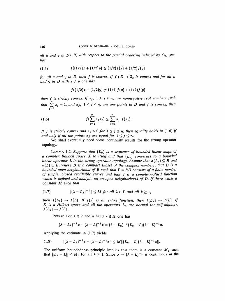
all x and y in D). If, with respect to the partial ordering induced by C2, onehas

for all x and y in D, then f is convex. If f : D -+ Z2 is convex and for all xand y in D with y one has

then f is strictly convex. If 1 j n, are nonnegative real numbers such

that and 1 j :!~, n, are any points in D and f is convex, then

If f is strictly convex and Sj &#x3E; 0 for 1 j n, then equality holds in (1.6) ifand only if all the points xj are equal for 1 j n.

We shall eventually need some continuity results for the strong operatortopology.

LEMMA 1.2. Suppose that (Lk) is a sequence of bounded linear maps ofa complex Banach space X to itself and that (Lk) converges to a boundedlinear operator L in the strong operator topology. Assume that a(Lk) C Banda (L) C B, where B is a compact subset of the complex numbers, that D is abounded open neighborhood of B such that r = a D consists of a finite numberof simple, closed rectifiable curves and that f is a complex-valued functionwhich is defined and analytic on an open neighborhood of D. If there exists aconstant M such that

for all

then j(Lk) --~ j(L). If is an entire function, then f (Lk) --~ f(L). IfX is a Hilbert space and all the operators Lk are normal (or self-adjoint),f (Lk) ~ f ~L)~

PROOF. For A E r and a fixed x E X one has

Applying the estimate in (1.7) yields

The uniform boundedness principle implies that there is a constant Mi suchthat L ~~ ~ M, for all k &#x3E; 1. (A - is continuous in the

247

operator norm, (1.8) implies that there is a constant independent of A e F,such that

~

for all

Inequality (1.8) and the fact that Lk ) --; L imply that

A version of the Lebesgue dominated convergence theorem now implies that

so f (Lk) - f ~L~.If .X is a Hilbert space, A E r and Lk is normal, it follows that A - Lk

and (A - are normal, so (see [36])

Because o(Lk) g B and r are disjoint compact sets, (1.10) implies that (1.7)is satisfied, so f (Lk) 2013~ f (L) by the first part of the lemma.

Finally, suppose X is a complex Banach space and f is entire. IfR = &#x3E; 11, we can take D = 2RI and for A E we

have -

so

Thus the first part of the lemma implies that f (Lk) --; f (L) in this case also. 0 .

REMARK &#x3E; . &#x3E;. The obvious analogue of Lemma 1.2 for the weak operatortopology is false. Let H be 12 and let 1 } be the standard orthonormalbasis for 1~ . For n &#x3E; 1, define a self-adjoint operator An : H - H by

for

for

One can easily prove that (An &#x3E; - 0, but (A 2) - I, the identity.

248

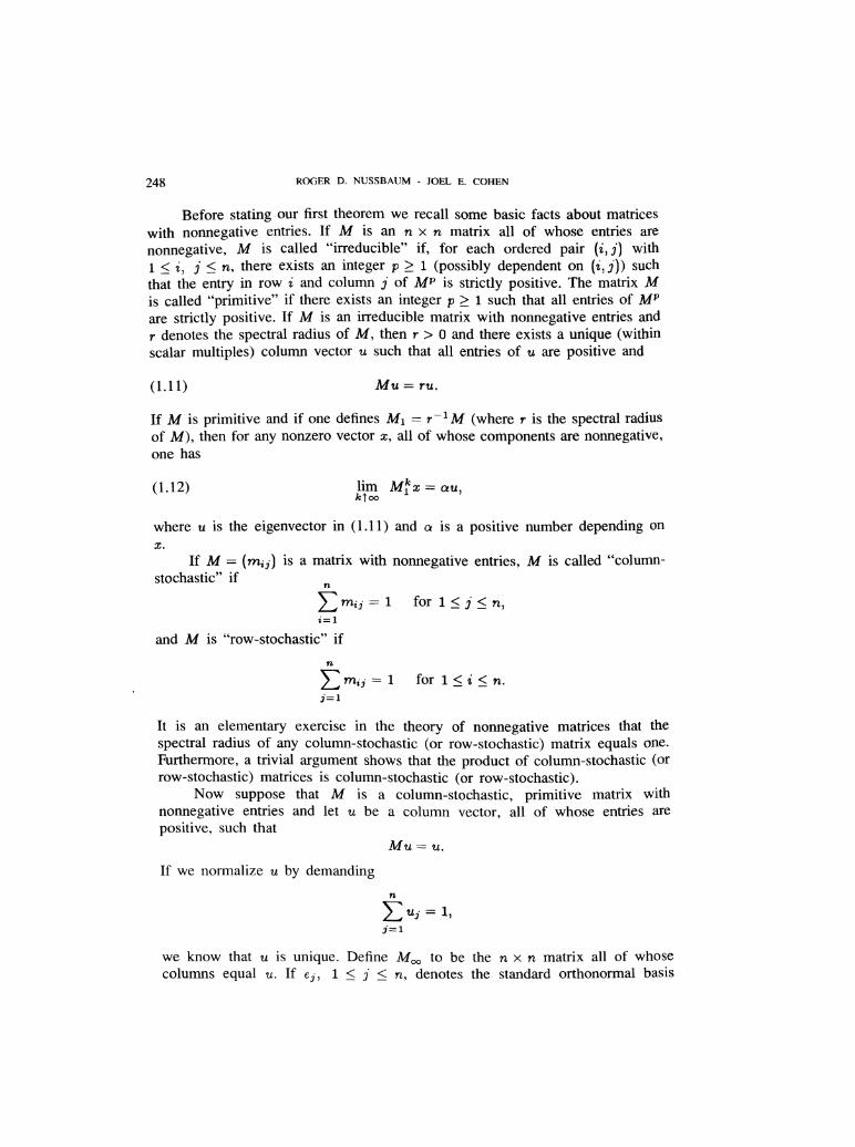
Before stating our first theorem we recall some basic facts about matriceswith nonnegative entries. If M is an n x n matrix all of whose entries are

nonnegative, M is called "irreducible" if, for each ordered pair ~i, j ) with

1 S i, i n, there exists an integer p &#x3E; 1 (possibly dependent on ~i, j ) ) suchthat the entry in row I and column j of MP is strictly positive. The matrix Mis called "primitive" if there exists an integer p &#x3E; 1 such that all entries of MP

are strictly positive. If ~VI is an irreducible matrix with nonnegative entries andr denotes the spectral radius of M, then r &#x3E; 0 and there exists a unique (withinscalar multiples) column vector u such that all entries of u are positive and

If M is primitive and if one defines Ml = (where r is the spectral radiusof M), then for any nonzero vector x, all of whose components are nonnegative,one has

where u is the eigenvector in (1.11) and a is a positive number depending onx.

If M = is a matrix with nonnegative entries, M is called "column-stochastic" if

n

for

and M is "row-stochastic" if

for

It is an elementary exercise in the theory of nonnegative matrices that the

spectral radius of any column-stochastic (or row-stochastic) matrix equals one.Furthermore, a trivial argument shows that the product of column-stochastic (orrow-stochastic) matrices is column-stochastic (or row-stochastic).

Now suppose that M is a column-stochastic, primitive matrix with

nonnegative entries and let u be a column vector, all of whose entries are

positive, such that

If we normalize u by demanding

we know that u is unique. Define Mco to be the n x n matrix all of whose

columns equal u. If 1 ~ j n, denotes the standard orthonormal basis

249

of 5i. n, we know that is the jth column of Mk, and because ~~ is

column-stochastic, ( 1.12) implies that

We conclude from the previous equation that, if M is column-stochastic and

primitive, then

If .~ is a cone in a Banach space X, let ~’ denote the cone which is then-fold Cartesian product of K. Let Y denote the n-fold Cartesian product ofX with any of the standard norms. If M is an n x n matrix with nonnegativeentries, M induces a bounded linear map W of Y to Y by

where

It is easy to check that W(C) C C, that W(C - { 0 } j ç C - { 0 } if no row of.~ is identically zero, and that (if KO is nonempty) Co if no columnof ~I is identically zero.

We are in a position to state our first theorem. For simplicity, we restrictourselves to the cone of p.s.d. bounded linear operators on a Hilbert space, butversions of the following theorem can be given for more general cones.

THEOREM 1.1. Let K denote the cone of positive semidefinite, self-adjointbounded linear operators on a Hilbert space H. Let C denote the n-foldCartesian product of K, C = K x K x ... x K. Let Y denote the n-foldCartesian product of X = £(H, B) with itself, Y == X x X x... x X. Supposethat f : CO --; CO is a continuous map and c~ : K° -; X is a continuous mapand Y by

Assume that for every A E CO there exist B E CO and positive reals a such that

and

250

for 0, where the partial ordering in (1.14) and (1.15) is induced by Cand f ~ is the j th iterate of f. Assume that there exists an n x n, primitive,column-stochastic matrix M such that, for every A E Co,

Let u denote the unique column vector such that all components of uiof u are positive and

and

and let 1ri denote the projection onto its ith coordinate. If, for A E Co,we define

. ,~, B ,., ’.. - ,

so ~~~~ _ 1ri f k (A)), there exists E E KO such that

Furthermore, for 1 i n, one has

PROOF. If u is the eigenvector in the statement of the theorem, define, forA = a function : by the formula

Inequality ( 1.16) implies, if A = (A,, A2, - - ., that

If we define Ek - ~ ( f k ~ .~ ) ~ , Ek - is an increasing sequence of bounded,self-adjoint operators, and ( 1.14) and ( 1.15) imply that Ek - El is bounded

251

above (in the partial ordering on K). Thus as k - oo, E with E - Eiself-adjoint. By iterating inequality (1.16) we see that, for any k &#x3E; 1,

The remarks preceding the theorem imply that given any e &#x3E; 0, there exists

Nx &#x3E; 1 such that for all k &#x3E; N1,

where is the matrix with all columns equal to u, and (1.22) means thatfor 1 i, j ~ n, the i, j entry of Mk is greater than or equal to the i, j entryof (1 - e) M,, - If k &#x3E; Ni, and 1 i n, it follows that

For a given x E H and e &#x3E; 0 there exists N2 such that

for

because .E~ --~ E. Combining inequalities (1.23) and (1.24) yields for k &#x3E;

N1 + ~2 ~

which implies that (using inequality (1.22) and recalling that isbounded in norm)

If, for some and some z, one has

then inequalities (1.26) and (1.27) imply

The above inequality contradicts the fact that

252

so inequality (1.27) must be false. We conclude from (1.26) that

Standard arguments using the polarization now imply that

There are several obstacles to using Theorem 1.1. The first problem, ofcourse, is to prove the existence of 0 and M as in Theorem 1.1 for examples ofinterest to us. We shall use the classical results of C. Loewner concerning theconcavity of order-preserving maps from the cone K of p.s.d. bounded linearoperators of a Hilbert space H to L (H).

However, even assuming that we can establish the hypotheses of Theorem1.1 in examples of interest, Theorem 1.1 provides inadequate information whenH is infinite dimensional. If H is finite dimensional, the weak, strong and

operator norm topologies on L (H) are identical, so Theorem 1.1 implies

for

If 0 is one-one with norm-continuous inverse, one concludes that

If ~Y is infinite dimensional, one would hope that there exists a p.d. boundedlinear operator G such that

for : -.

However, as Remark 1.1 shows, the weak operator convergence in ( 1.18) maybe very far from the strong operator convergence hoped for in (1 .29).

We now begin to address there deficiencies.If K is the cone of p.s.d. bounded linear operators in £(H) and H is a

Hilbert space, we need to know when certain maps defined on D = .H° are

order-preserving or concave or strictly concave. The first lemma is Loewner’stheorem [23, 24] concerning order-preserving maps on K’; an exposition ofLoewner’s theory is given in [ 16] .

LEMMA 1.3. (C. Loewner) Let K denote the cone of positive semidefinite,bounded linear maps of a Hilbert space H to itself. Suppose that f : (0, 00) -+ 3-is a continuous, real-valued map and that f has an analytic extension to

U = ~z c C : 0 or (Im(z) = 0 and Re(z) &#x3E; 0) ) such that &#x3E; 0

for all z such that Im(z) &#x3E; 0. Then the map A -+ f (A) for A E D == is

order-preserving with respect to the partial order induced by K.

253

Functions that satisfy the hypotheses of Lemma 1.2 are f (z) = log(z) and- zp, o p 1, and log(z) will be the example of most interest here.

One can give a simple and self-contained proof that if A, B E KO and A B,then B-1::; (although we shall not do so). Using this fact, we now provedirectly that the maps A - log(A&#x3E; and A ---&#x3E; AP, 0 p 1, are order-preservingon If ~’° and Et == (1 - t~ I + tE, where I denotes the identity map,then one can easily prove that

An algebraic manipulation gives

If A and .B are in KO B and At = and Bt = for 1, then Bt for 0 f t 1, so z for 0 t 1and

Using (1.31) and (1.32) one finds that log(A) log(B). That BP if A B

and 0 p 1 follows by a similar argument from the formula (see [21], p.286)

We also need concavity results for maps of ~° to

LEMMA 1.4. (Ando [3]) Suppose that K, Hand f are as in Lemma 1.3.Then, for A E K° , the map A - f (A) is concave and the map A - A f ~ A) is

convex (with respect to the partial ordering from K).Ando states Lemma 1.4 for finite-dimensional Hilbert spaces (Theorem 4

in [3]), but the same argument, based on Loewner’s theory, works for generalHilbert spaces.

Lemma 1.4 is not quite adeguate for our purposes. We need strict concavityand convexity results, and in fact we shall need a property (see Theorem 1.2below) analogous to the property of uniform convexity for norms,. Such resultswill follow from the strict convexity of the map A -~ A~ 1 for A E KO, and thisstrict convexity was proved independently by P. Whittle [34, Lemma 1] and I.Olkin and J. Pratt [29]. Whittle’s lemma is stated for finite-dimensional Hilbert

spaces, but the proof applies in general and yields the following lemma.

254

LEMMMA 1.5. ([34] and [29]) Let H be a Banach space and supposethat A, B c L (H) - If A is a real number such that 0 A 1 and A, B and

~ 1 - À)A + ÀB are one-one and onto, then

If H is a Hilbert space and K denotes the cone of positive semidefinite operatorsin £ (H), then the map A -4 A-1 of KG to KO is strictly convex.

By exploiting Lemma 1.5 we obtain the following sharpening of Ando’stheorem (Lemma 1.4). See also Bendat and Sherman [8].

LEMMA 1.6. Let f, K and H be as in Lemma 1.3. If there do not existreal constants a and (3 such that f (x) = 0, then for A c KO, athe map A -4 f (A) is strictly concave. If there do not exist real constants aand -y such that f (x~ - et -~- 1x-l for all x ~ 0, then A --~ is strictlyconvex on KG.

PROOF. Loewner’s theory implies that for A not a negative real, À i 0,

where a is real, Q &#x3E; 0 and p is a finite nonnegative Borel measure with supportin ( - oo, 0~ . If we assume that f (x) is not an affine map, then p is not the zeromeasure. From (1.35) and the identity

we obtain

The map is obviously concave and Lemma 1.5 implies that foreach t ~ 0 and for A G K° the map

is strictly concave so (1.36) implies A ~ f (A) is concave (Lemma 1.4). To

prove that A -- f ( A) is strictly concave, take A, K° B and

define

255

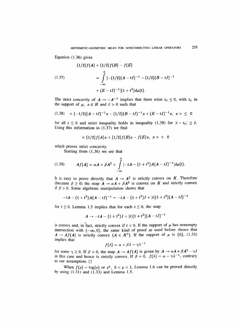
Equation (1.36) gives

The strict concavity of A -&#x3E; -A-1 implies that there exist to 0, with to inthe support of M, x E H and 6 &#x3E; 0 such that

for all t 0 and strict inequality holds in inequality (1.38) forUsing this information in (1.37) we find

which proves strict concavity.Starting from (1.36) we see that

It is easy to prove directly that A ~ A2 is strictly convex on K. Therefore(because Q &#x3E; 0) the map ~4 2013~ aA + is convex on K and strictly convexif B &#x3E; 0. Some algebraic manipulation shows that

for t ~ 0. Lemma 1.5 implies that for each t 0, the map

is convex and, in fact, strictly convex if t 0. If the support of /-z has nonemptyintersection with (- oc, 0), the same kind of proof as used before shows thatA -4Af (A) is strictly convex (A E KO). If the support Of /-z is fol, (1.35)implies that

for 0. If (3 &#x3E; 0, the map A --+ A f ( .A ) is given by A -- a A + in this case and hence is strictly convex. If/3=0, f ~ ~ ) = a - ~ a -1, contraryto our assumption. 0

When f ( z ~ = or 0 p 1, Lemma 1.6 can be proved directlyby using (1.31) and (1.33) and Lemma 1.5.

256

An immediate consequence of Lemmas 1.1 and 1.6 is:

COROLLARY 1.1. Let H be a Hilbert space. Suppose that A.1’, 1 j :5 rn,are bounded, self-adjoint, p.d. linear maps of H to H. If sj, 1 !,~ j S m, are

m

positive numbers such that E sj = 1, it follows thatj=l

Equality holds in (1.40) if and only if all the operators Aj are equal. If0 ci 1,

Equality holds in (1.41) if and only if all the operators Ai are equal.

REMARK 1.2. Suppose that Ai and sj are as above and that p and q arereal numbers such that 1 ~ p q. Defining a = pq-1 and Corollary1.1 implies

3

One only needs 0 p q to derive inequality (1.42). Since p &#x3E; 1, Lemma 1.3

implies that B --~ is order-preserving on K, so one obtains from (1.42)

For positive real inequality (1.43) is a classical result [20].Unfortunately, when H is infinite dimensional Lemma 1.6 is inadequate

for our purposes. We need to exploit strict concavity and strict convexity in amore quantitative way, analogous to the idea of uniform convexity for a norm.The next lemma illustrates the sort of uniform convexity we need for the caseof the strictly convex map A - A-1 when A is positive definite.

LEMMA 1.7. Suppose that Ai, 1 It m, are p.d., bounded linear mapsof a Hilbert space H into itself and 0.1 _ for 1 i m, where a and

{3 are positive reals. Assume that ak, 1 k m, are positive reals such thatm

2: ak = 1. Then, for 1 i, j ~ m,k=l

257

where the inequality refers to the partial ordering induced by the cone ofpositive semidefinite bounded linear maps.

PROOF. Because A - is convex, the left side of (1.44) is alwaysgreater than or equal to zero. To prove (1.44) it suffices (by relabelling) to

prove it when i = 1, j = 2.If A &#x3E; QI and B &#x3E; aI, then the spectral mapping theorem implies

A‘~ B‘1 and

and

Using inequality (1.45) in (1.34) gives

If we define inequality (1.46) givesand

If we define inequalityand the convexity of A --+ A - 11 give

Inequality (1.48) is precisely the statement of the lemma for i = 1 and j = 2.

0

The next theorem, when combined with Theorem 1.1, will enable us to

prove convergence in the strong operator topology.

THEOREM 1.2. Let K be the cone of positive semidefinite bounded linear

maps of a Hilbert space H into itself. Let C denote the m-fold Cartesian

product of K with itself. Thus C C Y, where Y is the m-fold Cartesian pro-duct of X = £(H) with itself. Assume that (B(k)), k &#x3E; 0, is a sequence in

C° , and write B ~ k ~ = ( B 1~ j , B~k ~ , ... ~ Suppose that ( 0, aa) - ’-I is

a real-valued function such that lim do(x)ldx = 0 and such that 0 has an:1:-+00

analytic extension to U = {z E C : Im (z) = 0 or (Im(z) = 0 and Re(z) &#x3E; 0))and &#x3E; 0 for all z such that Im(z) &#x3E; 0. Assume that there exist positivenumbers Ap 1 1 p m, such that

258

and that there are positive numbers a and {3 such that

Then for any i and j with 1 i, 3* m,

m

If there exist positive numbers ui, 1 z m, and E ~ KI such Ui == 14=1

and

then

If the restriction of 0 to an open neighborhood of ~0, oo) in C is one-one, then

PROOF. Loewner’s theory (see [16]) implies that if a ~ 0 and A is not a

negative real, then .

where cx1 is real, #1 &#x3E; 0 and p is a nonnegative, finite Borel measure. Usingthis formula one easily proves that the condition lim = 0 implies

x ---&#x3E; oo

that B1 = 0.We claim first that for all i and j, 1 ~ , j ~ m, one has

We shall prove this for 2 = 1 and j = 2, since the general argument is the

same. We obtain from (1.52) that

259

Inequality (1.50) implies that

so Lemma 1.7 and (1.53) give

The left side of (1.54) is assumed to approach 0 in the weak operator topologyas k - 00. Hence, for any x c H,

Now we return to (1.52). Using for the first time the fact that (31 = 0, weobtain

Because &#x3E; a7 for k &#x3E; 1 and 1 z m, it is easy to see that there exists

M1 such that

for all

It follows that for t -1

If we use this estimate in (1.56) and recall that J.1- is a finite measure, we findthat for any e &#x3E; 0 and any x E H, there exists a constant ~VI depending onlyon e, fi, Ilxll I and J.1- such that for all 1~ &#x3E; 1

260

On the other hand, the Cauchy-Schwartz inequality implies that

(1.55) implies that, for fixed x E H, the right side of (1.59) approaches zeroas k ---~ oo and hence is less than e/2 for l~ sufficiently large. Combininginequalities (1.58) and (1.59) gives, for l~ sufficiently large,

Using (1.56), we see that

As already remarked, the same argument shows - 0 for

any i and j.-

Suppose now that there exist positive reals ttl, U2, ... , Urn such that

and

For any fixed i, 1 i m, (1.60) can be rewritten as

which implies that

Finally, if 0 is one-one an open neighborhood of (o, oo) in C, then ¢~- ~is defined and analytic on an open neighborhood in C. Lemma

1.2 implies that

261

REMARK 1.3. The functions §(z) = log(z) and §(z) = zP, 0 p 1,

satisfy the hypotheses of Theorem 1.2.

REMARK 1.4. Suppose that K and H are as in Theorem 1.2, that f isas in Lemma 1.3 and that there do not exist real constants c~ and (3 such that

= for all x &#x3E; 0. Then Lemma 1.6 implies that A -+ f (A) is a strictlyconcave map from K° to f(~). Define f = 0 and assume that (1.49) and (1.50)are satisfied. if H is finite dimensional, it follows from the strict concavity off and a simple compactness argument that for all i and j, I

Thus, if H is finite dimensional, Theorem 1.2 follows trivially from Lemma 1.6.Theorem 1.2 only provides new information when H is infinite dimensional.

Theorems 1.1 and 1.2 are examples of convergence results in particularcones. However, one can give versions of Theorem 1.1 which are valid for

general classes of cones. Since we shall not use such results, we shall not provethem here, but it may be of interest to state the theorems.

THEOREM 1.3. Let K be a cone with nonempty interior in a finite-dimensional Banach space X. Let C denote the n-fold Cartesian product of K.Let Y denote the n-fold Cartesian product of X. Suppose that f : C’o -~ C’oand 0 : K° - X are continuous maps. For any y E CO assume that there existsz E C’ (dependent on y) and positive constants a and {3 such that

and

for all j 2: 0, where (D : Co -+ Y is defined X2, - - ., =

(4)(Xl), 0 (X2), - - ’, Assume that M is an n x n, primitive column-stochastic matrix with

nonnegative entries such that

for all

Let u be the unique positive column vector such that

If, for a given x E CO, we write

and

then there exists w E X, w dependent on x, such that

262

If eft is one-one, then w and

for

The proof of Theorem 1.3 is basically the same as that of Theorem l.l.One uses finite dimensionality to insure that the cone is "normal", i.e. that foreach u~ E K, the is bounded in norm. One also uses

finite dimensionality to guarantee that for every y E 2:: 1} is

precompact.To generalize Theorem 1.3 to certain infinite dimensional cones, we need

some terminology. Suppose that T is a topology on a Banach space X andthat X becomes a Hausdorff, locally convex topological vector space in theT topology and the T topology is coarser than the norm topology (so everyT -open set is open in the norm topology). If .K is a cone in X we shall saythat a sequence (Xj) of elements of K is monotonic increasing (with respectto the ordering induced by ~) if xi for all j &#x3E; 1, and we shall saythat is bounded above in the partial ordering induced by K if there existsw E K such that ~~ ~ for all j &#x3E; 1. If K, X and T are as above, we shallsay that K has the "monotone convergence property in the T topology" if everymonotonic increasing sequence in K such that (xi) is bounded above in

the partial ordering induced by K has a limit z in the T topology. Inthe situation of Theorem 1.1, X = is the cone of p.s.d. operators inX, T is the strong operator topology and K has the monotonic convergenceproperty in the T topology.

THEOREM 1.4. Let notation and assumptions be as in Theorem 1.3, exceptdo not assume that X is finite dimensional. Suppose that T is a topologyon X, coarser than the norm topology, such that X is a Hausdorff, locallyconvex topological vector space in the T topology and K has the monotoneconvergence property in the T topology. If u is the unique normalized positiveeigenvector of M and ( x lk ) ~ ~~k ~ ~ ... ~ xnk ~ ~ , there exists w e X so that

where convergence is in the T topology and ui is the ith component of u. IfL : ~ -~ ~ is any linear map such that ~(~~ &#x3E; 0 for all x E K and L is

continuous in the T topology, then

for

The proof of Theorem 1.4 is very similar to that of Theorem 1.1. If y G H, therole of L in Theorem 1.4 is served by L(A) = Ay, y &#x3E; for A E C(~).

263

2. - Convergence results for generalizations of the AG~

The original motivation for this paper was the problem of proving theconvergence of f k (,A, B~ for the maps

where .A and B are positive definite, bounded linear operators on a Hilbertspace. However, there are many generalizations of the classical Gauss-Lagrange-Legendre AGM, and to treat the extensions of these generalizations to the

operator-valued case in a reasonably unified way it is necessary to considermuch more general f than those in (2.1).

Thus, if .~ is a Hilbert space, let I~ denote the cone of p.s.d. operators in~ (.H~) . Let C denote the n-fold Cartesian product of K with itself. If Q E :t 1, call

n

a a "probability vector" if all components ai of o- are nonnegative and f (J = 1.If r is a real number, a is a probability vector and A = (At, A2 , ~ ~ ~ , An) E C°,define a map M,, : CO -+ ~° by

If r = 0, (2.2) does not make sense and we define

If A e C’°, then

THEOREM 2.1. Let K, H and C be as above. For each i, 1 i n, let

ri be a finite collection of ordered pairs (r, (1) such that r is a nonnegativereal and a is a probability vector. For each (r, a) E rs, let eir, be a positivereal number. Define f : CO by

denotes the jth component of f (A). Assume that

for

264

If ---+ 5~ denotes the projection onto the ith component of a vector,

define

and assume that the n x n matrix M = (mii) is primitive. Let u (u a

column vector) denote the unique probability vector such that Mu = u andlet ui = If, for A = (Al, A2, ..., An) E Co, we write

there exists E E KI such that

and

If (r, a) and (p, r) are both elements of fi for some i, 1:5 i n, then

If (r,a) E ri for some i and r &#x3E; 0, then for all p and q such that &#x3E; 0and &#x3E; 0 one has

If H is finite dimensional,

for :

If there exists (r, (7) E r fot- some i such that r &#x3E; 0 and all components of -5~are positive, then

for

PROOF. If A == (AI, A2,’ .., An) E Co and B == (B1, 82 &#x3E; ’ ° ’ Bn) * f (A)and if we define = Slj (A) and S~~ - 82i(A) by

265

and

we find that

The concavity of D -~ log D = 0 (D), for D E KO, implies that the right side of(2.17) is positive semidefinite. It follows that if 4D (A) is defined as in Theorem1.1 and § = log we have

for all

If A = (AI, A2," ., CO and a and Q are positive numbers such that

the spectral mapping theorem implies that for r &#x3E; 0

and

If a is any probability vector, it follows that

and

and by applying the spectral mapping theorem again we conclude that

A variant of this argument shows that (2.20) also holds if r 0. We obtain

directly from (2.20) that

266

or

A simple induction now shows that if A satisfies (2.19) and the notation is asin (2.8) then

for and

and (2.21) implies that

and i

Inequalities (2.20) - (2.22) verify the hypotheses of Theorem I.I, so

Theorem 1.1 gives (2.9) and (2.10). If H is finite dimensional, weak convergenceimplies norm convergence and by applying the exponential map to (2.10) weobtain (2.13).

If H is infinite dimensional, more care is necessary. If we replace A by= fk (A) and B by in (2.17) then

By using (2.10) and the fact that r 1, we conclude that the left sidei

of (2.23) converges to zero in the weak operator topology. Since is

p.s.d. and all summands of ~’~~ {A~k~ ) are p.s.d., (2.23) implies that

and

where (2.25) is satisfied if (r, Q) E Fj for some j and r &#x3E; o. We now applyTheorem 1.2 (recalling log z satisfies the hypotheses of Theorem1.2). Using Theorem 1.2 and (2.24) we find that (2.11) holds, and Theorem 1.2and (2.25) imply (2.12). If there exists (~, d) as in the statement of the theorem,we obtain from (2.12) that

for

Combining (2.9) and (2.26) we obtain as in Theorem 1.2,

for

267

and (2.14) now follows easily. DTheorem 2.1 provides insufficient information if H is infinite dimensional

and r = 0 for all (r, 0) E ri, 1 j ~ n. We consider this case separately inthe next theorem.

THEOREM 2.2. Let the notation and assumptions be as in Theorem 2.1.For 1 i ~ n, assume that if (r, (7) E Fi, then r = 0, so r i can be considereda finite set of probability vectors and we can write

Let u be the unique probability vector such that Mu = u. Assume that therear’e n - 1 pairs of probability vectors a(3’l and 7(i), 2 j n, such that and r(.i) E fi for some i depending on j and such that the n - 1 vectors,0(3) -= ~ {~ ~ -- 7(j), 2 j n, are linearly independent. Then for any A E CO,there exists E E KO such that

If n = 2 or if H is finite dimensional, (2.27) remains valid without theassumption that there exist vectors rxt~ ~ , 2 j n, as above.

PROOF. Theorem 2.1 implies that if C1 and T are any two probability vectorsin rj, 1 ~ j S n, then

or equivalently

If u is the eigenvector of M in the statement of Theorem 2.1, let ~V be

the n matrix whose first column is u and whose jth column is a131 for

2 j n. Equations (2.9) and (2.28) imply that, in the notation of Theorem2.1,

where

Because the components of aL1"), 2 ~ j ~ n, sum to zero and the componentsof u sum to one, it is easy to see that if we define u, the n vectors

268

(.t(j), 1 1 j n, are linearly independent. This implies that lV is invertible, andsince

we conclude that

which (with the aid of Lemma 1.2) gives (2.27).If ~ is finite dimensional, (2.27) follows directly from Theorem 2.1

without any knowledge of the vectors QLi). If n = 2 and T 1 or r 2 contains

more than one element, there is a nonzero vector = Q - T (a and r in

ri i for i = 1 or 2) and the theorem follows from our previous remarks. Thusassume that n = 2 and that r 1 and r2 each contains only one element, sayf1 = (a) and r 2 = {r}. If a = ( Q ~ , Q2 ) and r = ( T1, r2 ) , we find that

where

and M is assumed primitive. It follows that

and

where the column vector is the unique probability vector which is aneigenvector for M. One obtains the norm convergence of and from

the above equation. ~ 1 2

REMARK 2.1. Theorems 2.1 and 2.2 are not sharp results if H is infinitedimensional. It is possible that strong convergence of (A ~k)) 1 _ i n, is

valid with only the assumption that M is primitive, but we have not been ableto prove this.

It is worth noting that the conclusions of Theorem 2.2 remain valid if

there exist n - 1 linearly independent vectors 2 j n, such that

and

269

The vectors a(i) do not have to arise as in Theorem 2.2.

REMARK 2.2. Let notation and assumptions be as in Theorem 2.2 but donot assume the existence of probability vectors (1(j) as in Theorem2.2. Instead suppose that

for

Then the conclusion of Theorem 2.2 (in particular, (2.27)) still holds.To see this, note that M = is the matrix in Theorem 2.1 and that the

column vector u whose ith entry equals ui (uz as in (2.30)) satisfies Mu = u.Theorem 2.1 implies that for all r i, 1

and there exists E E K° so that

Because = u~ we have

so

Combining ~2.31 ) and (2.32) we obtain

so Lemma 1.2 implies

Using (2.33) we see that

which is the desired result.

270

Although the assumptions on M in Remark 2.2 are restrictive, theyare satisfied in some important applications. Remark 2.2 also provides furtherevidence that Theorem 2.2 is far from best possible.

It is useful in some applications to allow functions which are the

composition of functions like those in Theorems 2.1 or 2.2. One can giveanalogues of Theorems 2.1 and 2.2 for such functions even if H is infinite

dimensional, but for simplicity we restrict ourselves to the finite dimensionalcase.

THEOREM 2.3. Let K, H, C, 0 Theorem 2.1 and supposethat H is finite dimensional. Assume that f : C° --~ Co and g : CO arecontinuous maps and define h = g o f. Assume that for every A E C’° there existB E Co and positive reals a and f3 such that

and

for all j &#x3E; 0. Assume that there exist n x n column-stochastic matrices M andN with nonnegative entries such that for every C’

and

and MN is primitive. Then there exists E E KO such that, if hk(A) =

If 0 is one-one, one also obtains

PROOF. By using the hypotheses on f and g one finds

Thus h satisfies the hypotheses of Theorem 1.1, with ~N replacing M inTheorem I . I, and Theorem 2.3 follows immediately from Theorem 1.1. C7

COROLLARY 2.1. Let K, C and H be as in Theorem 2.1 and assume thatH is finite dimensional. Let f be as in Theorem 2.1, but do not assume thatthe matrix M defined by (2.7) is primitive. Suppose that g : Co is like

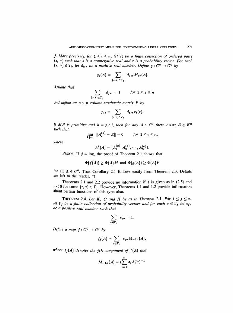
271

f. More precisely, for 1 ~ i n, let 7i be a finite collection of ordered pairs(s, r) such that s is a nonnegative real and r is a probability vector. For each(s, T) E Ti, let dis7 be a positive real number. Define g : ~’° --~ CO by

Assume that

and define an r~ x n column-stochastic matrix P by

If MP is primitive and h = g o f, then for any A E Co there exists E E KOsuch that

where,

PROOF. If 0 = log, the proof of Theorem 2.1 shows that

for all C’° . Thus Corollary 2.1 follows easily from Theorem 2.3. Detailsare left to the reader. 0

Theorems 2.1 and 2.2 provide no information if f is given as in (2.5) andr 0 for some (r, a) E ]Fj. However, Theorems 1.1 and 1.2 provide informationabout certain functions of this type also.

THEOREM 2.4. Let K, C and H be as in Theorem 2.1. For 1 j S n,let T’~ be a finite collection of probability vectors and for each a E ri let C iDbe a positive real number such that

Define a map f : CO -+ CO by

denotes the j t h component of f (A) and

272

for a = (a1, a2,’ .., and A = (AI, A2,..., An~, Define mii by

and assume the n x n column-stochastic matrix M = (mii) is primitive. Finallyassume that there are n - 1 pairs of probability vectors and r(i), 2 ~ j _ n,such that and are in ri for some i = i(j) and the n - 1 vectors

Q(i) = d ( a ) _ 2 ~ j ~ n, are linearly independent. Then for any A E Co,there exists E E KO such that

PROOF. Define §(z) = -z~1 and notice that O(z) satisfies the conditionsof Theorem 1.2 and that B - K°) is concave (see Section 1 ).Using the concavity of 0 one easily sees that if A E CO and .B =

and the right side of the above equation is positive semidefinite. The rest ofthe proof follows from (2.35) by using Theorems 1.1 and 1.2 as in Theorem2.2 and is left to the reader. D

REMARK 2.3. It is important to note that if Q is a probability vector, onecan write (for A E Co )

where 1" (i) is the probability vector with 1 at the ith position. Thus if f is

given as in (2.5) and r = 1 or r = -1 for each (r, rj, then by relabellingand redefining r i one can assume that f is as in Theorem 2.4.

By using the above remark and Theorem 2.4 we obtain the followingcorollary.

COROLLARY 2.2. Let the notation and assumptions be as in Theorem 2.4except do not assume the existence of n - 1 pairs and as in Theorem2.4. Assume that there exist n positive numbers d j , 1 j ~ n, such that 11 (A),the first component of f (A), satisfies

273

Then for any A E Co, there exists KO such that

PROOF. As noted in Remark 2.3, write

where ii comprises the n probability 1 j n, and has 1in the j th position. Then

are n - 1 linearly independent vectors and the corollary follows from Theorem2.4. C7

A very special case of Corollary 2.2 is an arithmetic-harmonic mean (thecase a = ~Q -- 1/2 below) which has been considered by Fujii [19].

COROLLARY 2.3. Let H be a Hilbert space, K the cone of positivesemidefinite operators in ,~ (H~, and C = K x K. If a and f3 are real numberssuch that 0 a, /3 1, define f : C° --~ C° by

If (A, B) E C’°, there exists E E KG such that

Although we shall not prove this here, one can prove convergence in theoperator norm under the assumptions of Corollary 2.3.

Similarly, as a direct corollary of Theorem 2.2 we obtain an operatorvalued extension of the AGM of the type suggested by (2.1).

COROLLARY 2.4. Let K, C and H be as in Corollary 2.3. If a are

real numbers such that 0 a, p 1, define f : C’° --; CO by

Then for any (A, B) E CO, there exists E E KO such that

PROOF. Since A can be written as exp(log A) and similarly for B, themapping f is of the form considered in Theorem 2.2 and (in the notation of

274

Theorem 2.2) n = 2.,One easily checks that

so M is primitive and the corollary follows from Theorem 2.2. 0If A and B are positive real numbers in Corollary 2.4 and a = 1/2,

it was known classically (see [13]) that one can express the limit of fk (A, B)in terms of an elliptic integral. However, as D. Borwein and P.B. Borwein havepointed out [ 11 ], for general a and 03B2 (even if a = Q) there is no known integralformula for the limit of f k (A, B).

There are many other classical variants of the AGM. Carlson [13] givesa unified treatment of some of these results. In one example, Carlson defines(for a and 6 positive reals)

and

He then defines a map by

The case i = 1 and j = 3 is usually attributed to Borchardt (see [6], [9]). Onecan prove that

and Carlson gives explicit integral formulas for Lii (a, b) .We wish to generalize the above convergence results to pairs of p.d.

bounded linear operators .A and B on a Hilbert space. If A and B commuteor if, as in Section 4 below, one uses a different analogue of the square rootof the product of two positive numbers, one can also generalize the integralformulas However, we shall only carry this out for the case of theAGM in Sections 3 and 4 below. Thus let H be a Hilbert space and K thecone of p.s.d. operators in ,~ ~H) . If A, B E KO and r is a real number suchthat 0 r 1, define

Define a map ~’ of K° x K° into itself by

where

275

It will always be assumed that

COROLLARY 2.5. Let H be a Hilbert space and K the cone of p.s.d.operators in £(H). Let Cj and 0 i :5 4, be nonnegative real numbers

satisfy (2.41 ) and let 1i and 6j, ~ j S 4, be real numbers such thato 1j, 8j 1 , for 2 j 4. In addition assume that Cj 1 and dj 1 forj = 0 and j = 1. Define a map f of KI x KI into itself by (2.36) - (2.40).Then for any (A, B) E KO x Ko, there exists E E KO such that

PROOF. Define D = ~f x K x K and define a map g : D° - D° by

where C is now an arbitrary element Ko, A1 and Bl are given by (2.38) and(2.39) respectively and

If 7r projects D’ onto K° x K° so that

an easy induction argument shows that if (A, B, C) E Do andthen

for all

Thus to prove Corollary 2.5 it suffices to prove that for any (A, B, Dothere exists E e KO such that

276

The map g is of the form in Theorem 2.2 (whereas f is not), and one couldtry to apply Theorem 2.2 and Remark 2.1. Such an approach requires slightlystronger assumptions than we have made, so we shall use a somewhat differentargument.

We first eliminate some trivial cases. If we have

so d3 = d4 = c3 = c4 = 0, is a function of (A, B), the function beingof the type considered in Theorem 2.2. Thus we are in the case n = 2 of

Theorem 2.2. The assumption that cj 1 and dj 1 for i = 0 and 1 insuresthat the corresponding 2 x 2 matrix M has all positive entries. Thus we aredone if (2.46) is satisfied.

Similarly, if

( A1, Cl ) is a function of (A, C) and the corollary follows easily from the casen = 2 in Theorem 2.2. Also, if

is a function of (B, C) and we return to the case n = 2 in Theorem2.2.

Thus we can assume that (2.46), (2.47) and (2.48) are all not satisfied.Let M be the 3 x 3 column-stochastic matrix defined as in Theorem 2.2 for our

map g. One can easily check from the defining equations for g that the thirdcolumn of M is the arithmetic average of the first two columns. Because c~ 1

and di 1 for j = 0 and j = 1, each of the first two columns of M has at mostone zero entry. If the first entries of columns one and two of M are both zero,then (2.48) is satisfied, contrary to assumption. Similarly, if the second entriesof both columns one and two of M are both zero, (2.47) is satisfied, contraryto assumption. Finally, if the third entry of column one of M equals zero andthe third entry of column two of M equals zero, (2.46) is satisfied, contrary toassumption. Thus the zero entry of column one of M (if it exists) is never in

the same position as the zero entry of column two, so the third column of M,being the arithmetic average of columns one and two has all positive entries.Using this information, one easily checks that M2 has all positive entries.

If u is the probability column vector such that Mu = u and if we write

Theorem 2.1 implies that there exists E E ~° such that

277

and log Ak, log Bk and log Ck converge weakly to log E. Because

we conclude that

Using (2.50) and Theorem 1.2 we conclude that

Because Ck = (Ak + Bk)/2 for k &#x3E; 1, we have for k &#x3E; 1

(log log log (log Ak, log Bk, log Ck)M&#x3E; (log Ak, log Bk, (log Ak)/2 + (log Bk)/2)M.

Using the above inequality we find that for k &#x3E; 1

where P = has elements

Because each of the first two columns of M has at most one zero entry, allentries of P are positive, and P is obviously column-stochastic. If v is the

unique column probability vector such that Pv = v, Theorem 2.1 implies

for some K° . One obtains directly from (2.51) and (2.52) that

so Lemma 1.2 implies

There are many other classical generalizations of the AGM. For example,G. Borchadt (see [6] and [9] for references) studied the map

278

where

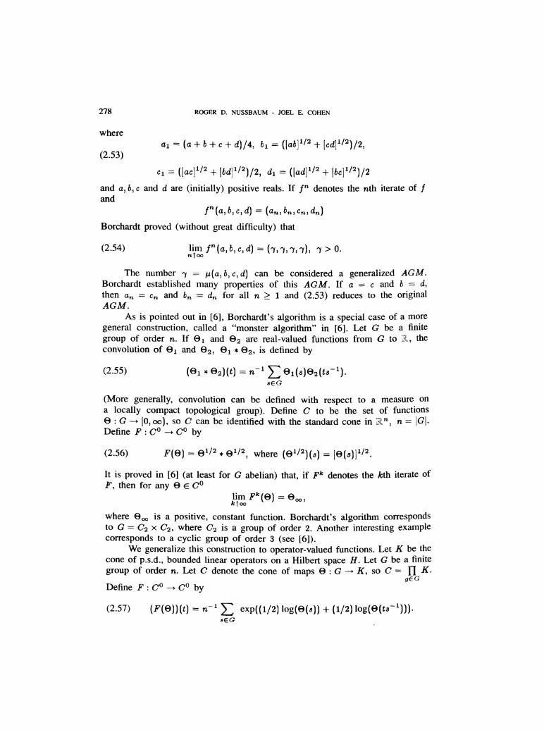
and a, b, c and d are (initially) positive reals. If f n denotes the nth iterate of fand

Borchardt proved (without great difficulty) that

The number 1 = J.l(a, b, c, d) can be considered a generalized AGM.Borchardt established many properties of this AGM. If a = c and b = d,then an = cn and bn ---. dn for all n &#x3E; 1 and (2.53) reduces to the originalAGM.

As is pointed out in [6], Borchardt’s algorithm is a special case of a moregeneral construction, called a "monster algorithm" in [6]. Let G be a finite

group of order n. If 81 and 82 are real-valued functions from G theconvolution of ~1 and 62 82, is defined by

(More generally, convolution can be defined with respect to a measure on

a locally compact topological group). Define C to be the set of functions~ : G --f [0, oo), so C can be identified with the standard cone = .

Define F : by

It is proved in [6] (at least for G abelian) that, if Fk denotes the kth iterate ofF, then for any ~3 E C°

where Boo is a positive, constant function. Borchardt’s algorithm correspondsto G = ~’2 x C’~, where ~’2 is a group of order 2. Another interesting examplecorresponds to a cyclic group of order 3 (see [6]).

We generalize this construction to operator-valued functions. Let K be thecone of p.s.d., bounded linear operators on a Hilbert space H. Let G be a finitegroup of order n. Let C denote the cone of n K.

gE GDefine F : C° - CO by

279

This reduces to (2.56) when (3 is a real-valued.

COROLLARY 2.6. Let the notation be as in the immediately precedingparagra,ph. Then for any e E C’,

where 800 depends on e and t~~ : G - K’ is a constant function.

PROOF. The cone C can be considered as the n-fold Cartesian productof K, and with this identification the map F is a special case of the mapsconsidered in Theorem 2.2. We shall derive Corollary 2.6 from Remark 2.2.

Define § : ~° -~ X = ,~(~~ by r~~~) = log A and if Y denotes the Banachspace of maps from G to X, define 4P : Co --~ Y by

for all Î

Applying ø to (2.57) and using the facts that

and ø is concave gives

or

where M is the doubly stochastic matrix with all entries equal to n-1. Thuswe are in the situation of Remark 2.2 and the corollary follows. C~

1~s already noted, we immediately obtain the operator analogue of

Borchardt’s algorithm from Corollary 2.6.

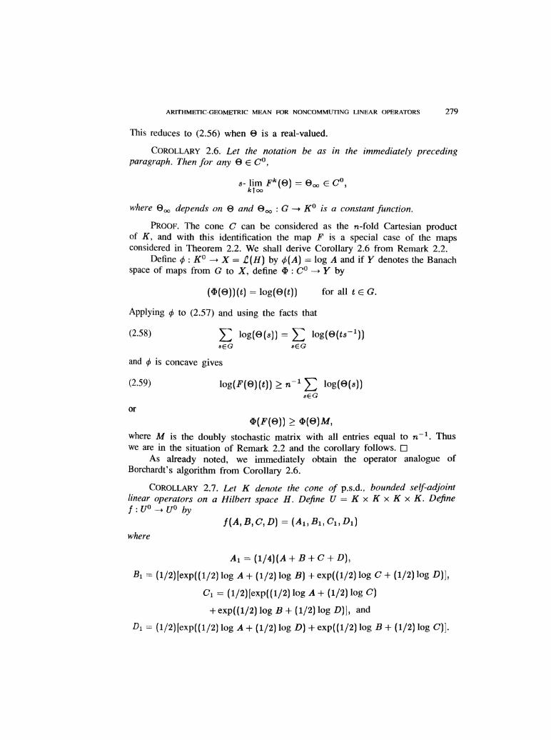
COROLLARY 2.7. Let K denote the cone of p.s.d., bounded self-adjointlinear Operators on a Hilbert space H. Define U = K x K x K x K. Define

where

280

Then if f - (A, B, C, D) = (Art, Bm, Cm, Dm), there exists E E KO such that

Many other generalized means have operator-valued versions that can beanalyzed by our methods. We mention only two more examples. Borchardt andSchwab (see [6]) considered the map

and the corresponding mean given by

Carlson [12] observed that the Borchardt-Schwab algorithm is naturallyembedded in an algorithm involving three variables. Given positive numbersa, band c, define Q, (3 and y y by

and define == where

and (

If = Carlson proved that

He related the limit to certain integrals. If b = c, then bn = cn for 1

and one recovers the Borchardt-Schwab algorithm.To generalize Carlson’s algorithm to operator-valued maps, let .K denote

the cone of p.s.d., bounded self-adjoint linear maps of a Hilbert space H toitself. Define E = K x K x K. Define f : E, - El by

where

and

281

COROLLARY 2.8. If f : .~° --&#x3E; Eo is defined by (2.60) - (2.62), then forany (A, B, C) c EO,

where D E K°.

PROOF. Define 4) (A, B, C) == (~(~), ~(~), ~(C)~ for (A, B, C) E E°,where ~(~) = log A for A E K°. It follows easily from the concavity of logthat

.

where

The reader can easily verify that the other hypotheses of Theorem 1.1 hold, soif C) = (Ak, Bk, Ck), there exists D E K° such that

and

The defining equation for f gives

The left side of (2.66) converges to zero in the weak operator topology, soTheorem 1.2 and (2.66) imply

(2.65) and (2.67) give

282

and the corollary follows from (2.68) with the aid of Lemma 1.2. 0A final example is an algorithm of Meissel (see [6]). For positive real

numbers a, b, c define

If K is the cone of p.s.d., self-adjoint linear operators on a Hilbert space Hand E = K x ~‘ x K, one can define a map f : ~° -~ EO which is an analogueof the map in (2.69), namely,

where

COROLLARY 2.9. If Hand K are as above and f : L~’° --~ Eo is definedby (2.70)-(2.71), then for any (A, B, C) E Eo, there exists D E KO such that

PROOF. Corollary 2.9 follows by essentially the same argument used toprove Corollary 2.8 and is left to the reader. p

3. - Some elementary properties of the arithmetic-geometric mean

In this section we shall establish some basic properties of

where

Much of what we say extends to the more general examples considered in

Section 2, but for simplicity we shall restrict ourselves to the above case or,occasionally, the "monster algorithm" of Corollary 2.6.

We begin with some generalities. If X is a complex Banach space, Gis an open subset of X and f : G --3 X is continuous, f is called analyticif, whenever Br(u) = {i/ : liy - ull rl C E X* is a complex linear

283

functional and v E X is such that Ilvll = 1, then A - + A v)) is complexanalytic for all A c C such that a ( r.

If X is a complex Banach space, let Y denote the n-fold Cartesian productof X and for Y = ( yl , y2, ~ .. , define a seminorm p(y) by

Then p(y) = 0 if and only if where

LEMMA 3.1. Let X, Y, p and S be as above. For yo E Sand 6 &#x3E; 0 let= ly c Y : 11 y - yO 11 c ~ ~ = U and suppose that f : U - Y is an analytic

map such that = y° . Assume that there exists c 1 and a constant ksuch that

and

for all y E U. Then there exists r &#x3E; 0 such that f - (y) E U for all m &#x3E; 1

whenever y E and f m (y) converges uniformly in y E B,. ( y° ) as m - 00to a limit g(y) c- S such that f (g(y)) g(y). The map y - g(y) is complexanalytic on

PROOF. For definiteness, define 11 y = max If a sequence of analytic1:5in

functions converges uniformly on an open set G to a limit g, g is analytic on G.Thus, in our case, to prove g is analytic on Br (yO) for some r &#x3E; 0, it suffices

to prove that 1m (which is analytic) is defined and converges uniformly onBr (yO).

Take ro &#x3E; 0 such that

and note that p (y) 2 ro for all y e Define

and assume that if y E then for 0 i m and for 0 j m. Then (3.5) and (3.6) imply that

284

so

By mathematical induction we find that for all j &#x3E; 1.

If y E and m and v are positive integers, m v, then

(3.7) shows that (fm(y)) is a Cauchy sequence with limit g ( y) . If v --~ oo in(3.7), then

so the convergence is uniform in y E Obviously g(y) and

f (g(y)) = g(y), and because p(f (9(~))) -- ~~g(~)) ~ p(g(y)) = 0and g(y) E S. ~

Under the hypotheses of Lemma 3.1, convergence is "linear", whereasfor the examples of interest to us, convergence is actually "quadratic" (see[35], Chapter 12 for definitions) and hence extremely rapid. The next lemmadescribes the situation we shall actually encounter.

LEMMA 3.2. Let the notation and assumptions be as in Lemma 3.1 exceptinstead of assuming that f satisfies inequality (3.5), suppose that there exists aconstant M such that

for all y E U. Then the conclusions of Lemma 3.1 are still valid.Fuf-thermare, if 6 in Lemma 3.1 is so small that

then, setting u = um =

285

for Bra and m &#x3E; 0.

PROOF. By decreasing s we can assume that (3.9) is satisfied on (3.8) then implies that (3.5) is satisfied, so the conclusions of Lemma 3.1 hold.An easy induction shows that if we define uj = 23, then

If we use (3.6) and (3.11) we find

If we define p = c2m, it is easy to see that

and (3.12) and (3.13) give (3.10). 0Next we establish a theorem which, as we shall see later, is applicable to

the "monster algorithm" of Corollary 2.6.

THEOREM 3.1. Let X be a complex Banach space and Y the n-foldCartesian product of X with itself. Let p and S be as defined in (3.3) and(3.~).

Suppose that V is an open subset of Y and f : V ---~ Y is a complexanalytic map. Define W C V by

(The element u in (3.14) depends on y). For each u E V t1 S, assume thereexist positive constants c, ~ and k (dependent on u) such that c 1 and

for all y E B6 (u) _ {y : Ily-ull 6}. Then W is an open set and

is an analytic function on W.

286

PROOF. If y E W , select u E V n S such that f’n (y) converges to u. If

and k are as above, select ro as in Lemma 3.1, so that if w E then

E B~ ( u ) for 1 and

where g is an analytic function on B,, (u). There exists an integer l1~ so

that and by continuity of f N, there exists 61 &#x3E; 0 so that

E for all z such 61. It follows that bi,

Thus we see that W is open. Also, because the restriction of g to (u~ is

analytic (by Lemma 3 .1 ) and f N is analytic, (3.16) implies that g is analyticon an open neighborhood of y. 0

The argument of lemma 3.2 shows that to verify (3.15) in Theorem 3.1,it suffices to verify (3.f ) and (3.8). To accomplish this for the examples ofinterest to us we need the next fact.

LEMMA 3.3. Let H be a Banach space and X = £(H). Suppose that

Ao E X and a(Ao) n (-oo, 0] is empty. Then there exists 8 &#x3E; 0 and M &#x3E; 0 suchthat (1) for all A E Bs ( Ao ) , the open 8 ball about is emptyand (2) if are any elements of and Ql,a2,"’,am are

positive reals such that E Qj = 1, thenj=l

PROOF. By assumption, (1 - t) Ao + tI is invertible for 0 t 1, and

by continuity of the map A - A-1 on the set of invertible linear operators,11[(1 - t) Ao + tI] -’ 11 is uniformly bounded for 0 t 1, say by a constantMI. If [)A - Ao [) 6 and 6 (2M,)-’, then writing Aot = tAo + (1 - ~)~ andAt = tA + ( 1 - t) I for 0 t 1, one has

so At is invertible (the product of invertible operators) and

287

To prove (3.17), first assume that m = 2 and take A and B in and ci so that 0 ci 1. If C E and we write Ct = I + t ( C’ - I) for0 - t :5 1, we have

If we take C = a A + ( 1 - o:)J3, C = A and C = B in (3.18), we find aftersimplification that

where

By using Lemma 1.5 and (1.34) we obtain

Using the identity

in (3.21) and simplifying we find

Since and

we obtain from (3.22) (using also that a(1 - a) ~ (1/4)) that

288

Using this estimate in (3.19) yields

Our argument actually shows that if U is an open neighborhood of Ao suchthat ((1 - t)A+ exists for all A E U and 0 t 1 and

then (3.23) is satisfied.We now proceed by induction. We have proved the lemma for m = 2, the

constant ~ in (3.17) being Assume for some m &#x3E; 2 that we have provedthe lemma for m - 1 and that the constant M in (3.17) can be taken to be Let Aj and OJ, 1 j m, be as in the statement of Lemma 3.3 and define

-

and a = ai. Then A, B G and (3.23) gives

Using the Cauchy-Schwarz inequality,

On the other hand, the inductive assumption implies

289

Combining (3.24) - (3.26) we find that

so the lemma has been proved by induction. 0With these preliminaries we return to the "monster algorithm" of Corollary

1.5.

THEOREM 3.2. Let H be a complex Banach space, let X = l(H) and letU == n (-00,0] is empty}, where a(A) denotes the spectrum ofA. If G is a finite group of order n &#x3E; 2, let Y denote the Banach space ofmaps from G to X, so Y can be identified with the n-fold Cartesian productsof X. E Y : 8(8) E U for all s E G ~ and define F : ~ --3 Y by

Define S to be the set of constant functions in Y and define W by

where F" denotes the mth iterate of F and W depends on e. Then W is anopen subset of Y. If g(e) is defined by

for W, the map e ~ g(8) is analytic. The convergence in (3.29) is

quadratic. If H is a finite dimensional Hilbert space, W contains where

is positive definite and self-adjoint for all G~.

PROOF. Select B11 E V n S. By Theorem 3.1 it suffices to prove thatthere exists 6 &#x3E; 0 such that (3.6) and (3.8) are satisfied for all e e B6 (W) =

Y : o}. The map A - exp(A) is C1 with boundedse

Fréchet derivative on bounded sets in X, so the map A --&#x3E; exp(A) is Lipschitzianon bounded sets. Similarly, for 6 small enough, A - log A is Lipschitzian onB~ ( ~) . Thus to prove that F satisfies inequality (3.8) on for some 6 &#x3E; 0,it suffices to prove that there exists M such that

for all e E B,6 (IF), where, for a E Y,

290

We know that for ~ E V

Using Lemma 3.3 we find that there exists 6 &#x3E; 0 and a constant such that

for all O E 86 (W) one has

where

Because the map ~4 -~ exp ~1 is Lipschitzian on bounded sets, we find from(3.32) - (3.34) that there exists a constant M2 such that

for all Q E 86 (T) - It follows from (3.35) and the triangle inequality that forall

so

It remains to prove (3.6). By using the Lipschitz nature of ~4 ---~ exp Aand A ~ log A on appropriate sets, it suffices to prove that there exist 6 &#x3E; 0

and a constant l~ such that

for all 0 E 86 (’11). By using (3.35) and the triangle inequality we see that

291

If M3 is chosen so that p(log 9) M3 for all e E (3.37) implies that

The final assertion of Theorem 3.2 follows immediately from Corollary 2.6 andthe fact that strong convergence implies norm convergence in finite dimensions.0

The AGM of Section 1 is a special case of the monster algorithm whenthe group is of order 2. Thus:

COROLLARY 3.1. Let H be a complex Banach space, X =

andY=XxX. Let U= ø} and letV == I (A, B) E Y : A E U and B E U}. For (A, B) E V, define f(A, B)by

Define W by

Then W is open and if g(A, B) is defined by

for (A, B) E W, then (A, B ) ~ g (A, B) is analytic. If H is a finite dimensionalHilbert space, W contains WI, where

Wi = I (A, B) : A and B are positive definite, bounded and self adjoint}.

PROOF. Corollary 3.1 follows from Theorem 3.2 if one observes that

Aoo = Boo whenever

for some Aeo E U, Beo E U. This is because the form of f implies

REMARK 3.1. It would be interesting to obtain more information about theset W in Corollary 3.1, even for H finite dimensional. For instance, is it truethat almost every pair (A, B) E Y (with respect to Lebesgue measure) belongsto ~’? Numerical studies for dim H = 2, 3, 4, 5 suggest this may be true.

If H is a Hilbert space and L (H) = X, A is called accretive ifRe &#x3E; &#x3E; 0 for and A is strictly accretive if there exists

292

et &#x3E; 0 so that Re Ax, x for all x E H. It is natural to conjecturethat for almost every pair (A, B) such that A and B are strictly accretive onehas (A, B) E W. However, one can give an example of 2 x 2 upper triangularaccretive matrices A and B such that if (Ai , Bi ) = f (A, B), Bl is not accretive.This, of course, does not disprove the conjecture.

Because f is homogeneous of degree 1 and

it is obvious that if (A, B) E W, then (AA, AB) E W for all A &#x3E; 0 and

E W for all invertible S. If H is finite dimensional and Aand B are both upper triangular matrices with spectrum strictly in the right halfplane, one can also prove that (A, B) E W, though we omit the proof.

There remains one easy case in which one can prove (A, B) E W, thatis, when AB = BA. Stickel [32] has discussed the commutative case when Aand B are matrices, but his argument seeems incomplete. We shall sketch anapproach which works when H is a complex Banach space.

Suppose that H is a complex Banach space and A, B E £(H) = X arecommuting linear operators. Consider the algebra .~ of complex-valued functionsg which are defined and analytic on Ug x Vg, where U, is an open neighborhood

and Vg is an open neighborhood of Two such functions g, and

92 are identified if they agree on U x V, where U and V are some open setscontaining a { Aj and a (B) respectively. If g E ~ is defined on U x V, let r 1 ç Ube a finite union of simple, closed rectifiable curves which contain Q {Aj in theunion of their interiors, and similarly for F 2 g V. Define g (A, B) E by

The operator g (A, ~3 ~ defined by (3.38) does not depend on the particular choiceof f1 and F 2 as above. Furthermore, the map g -~ g ~ A, B) E C (H) is an algebrahomomorphism from to ~(77). The proof of this fact is a minor variant ofthe argument (see [33], [36]) for defining the functional calculus for a singleoperator and will not be given here. In fact, the functional calculus summarizedby (3.38) is a special case of a much more subtle functional calculus developedby Shilov, Waelbrock, Arens-Calderon and Arens: see [7] for references. If

gn : U x V -+ C, n &#x3E; 1, is a sequence of analytic functions and gn convergesuniformly on U x V to g, then by using (3.38) one can easily see that B)converges in norm to

If ~J and V are as above and g : U x V - C is analytic, then by usingthe fact that g - g(A, B) is an algebra homomorphism and that the functionidentically equal to 1 goes to the identity in ,~ ~H) one can see that

293

Applying (3.39) to g (z, w) = (z + w) / 2 and g (z, w) = gives

and

We can also use the composition of analytic functions. If g E A and h isanalytic on an open neighborhood of g(a(A) x a (B)) 9 C, then i = h o g e Aand (3.39) implies that h(g(A, B)) is defined and one can prove, as for thefunctional calculus in one variable, that

If g(z, w) = (g, (z, w), g~ (z, w)), where gj E A for j = 1, 2, one can define

and it is easy to see that A1 and BI commute. If Wi is an open neighborhoodof x o, (B)) and h : WI x W2 - C 2 is analytic, then j = h o g isdefined on Uo x ~o, where II~ is an open neighborhood of and ~o anopen neighborhood of a (B) and

Now define open subsets G C C and 0 9 ,G(H) by

and

Let z denote the standard single-valued branch of the square root function:

where and

It is easy to see that for z and E G

Thus, using the properties of the functional calculus, we see that if ~A, B) E0 x 0 and A B == BA, then

If 0 and z is not a negative real}, then if (A, B) c 0 x 0,(3.40) implies that a(AB) ç G 1, and the spectral mapping theorem implies that

294

(3.40) also implies that a((A+ B)/2) C G if (A, B) E 0 x 0. It follows that ifwe define W = {(A, B) E 0 x 0 : AB = BA) and if F : W -~ .C(H) x C(H) is

defined by

then F(W ) C W. Thus if (A, B) E W we can consider Fm (A, B), where Fmis the mth iterate of F : V~ ---~ W.

On the other hand, if we = ( ( z + w ) / 2 , (z w) 1/2), then

f (C x G) 9 G x G. For (A, B) E W, we have f (A, B) = F (A, B), where f (A, B)is defined by (3.38). If 1m denotes the mth iterate of f : G x G --~ G x G,the previously mentioned properties of the functional calculus (particularly therules of composition) imply that

where the left side of (3.48) is defined by (3.38) with g = 1m.The classical theory of the AGM implies that for all (z, w) E G x G one

has

where

and that the convergence in (3.49) is uniform on compact subsets of G x G. Itfollows from (3.49) and (3.50) that

where g(A, B) in (3.51) is defined by (3.38) and g is as in (3.50). Finally, arelatively simple argument (which we omit) shows that

where the right side of (3.52) is interpreted as an improper Riemann integralwith values in £(H). Thus:

PROPOSITION 3.1. Let H be a complex Banach space,

and z is not a negative real)

295

and

then F(W) C W and

where g(A, B) is defined by (3.52).

4.. Alternate definitions of the AGM

In the previous section we have considered one type of generalization of theclassical AGM. However, there are many possible "reasonable" generalizationsof the AGM to pairs of bounded linear operators ( A, B ~ . In fact, as we shallsee later, there is a continum of arithmetic-geometric means, all of which aredefined when A and B are p.d. and self-adjoint, all of which give the samevalue when AB = BA, but all of which in general give different values .when

BAWe begin with an observation which was made to the authors by the

referee of our earlier paper [14]. If A and B are n x n Hermitian, positivedefinite matrices, define f (A, B) by

where ( B ~ ~ A~ 1 ~~ is defined by { 1.1 ). The referee remarked that, despiteappearances, the expression B(B-1 A) 1~2 is symmetric in ~4 and B and is

positive definite and self-adjoint. Furthermore, he observed that for A and Bp.d. and self-adjoint, it is relatively easy to prove that

where C is p.d. and self-adjoint.If .A and B are p.d., self-adjoint bounded linear maps of a Hilbert space

.~ to itself, J. Fujii [19] has defined a map g by

296

where A#B is a "geometric mean" introduced by Pusz and Woronowicz [31].Pusz and Woronowicz proved (see also Theorem 2 in [3]) that

Fujii proves that if A and B are p.d., self-adjoint operators in C (H), then

where C is p.d. and self-adjoint.We shall show first that

where f (A, B) is defined by (4.1) and g (A, B) by (4.3) and (4.4). This willimply of course that the limits defined in (4.2) and (4.5) are equal. We beginwith a trivial lemma.

LEMMA 4.1. Let H be a Hilbert space and suppose the A, B E £(H) andA and Bare p.d. and self-adjoint. Then a(AB) = spectrum of AB C (0, aa).

PROOF. Because a(AB) = and

is p.d. and self-adjoint, the lemma is proved. 0We now recall some basic fact about the functional calculus for linear

operators. If H is a Hilbert space, A E £(H) and f is analytic on an openneighborhood U of a(A) u a (A*) and f (‘z) = f (z) for all z in U, then

f ( A* ) - (f (A))’. If H is a Banach space, A e C (H), f is analytic on anopen neighborhood of and ~’ is invertible, then

We shall always use the standard single-valued branches of z’ and log z. Thusif

and z is not a negative real},

and 181 w, then

and log ;

It follows that if H is a complex Banach space, A E and a(A) C Gi,then for any real numbers A and

297

and if A and p are real numbers such that 1 (so zl E G1 for all z E G1)

LEMMA 4.2. Suppose H is a complex Banach space and A and B are inZ(H), B is invertible and a(B-’A) 9 Gi, where G1 is as in (4.7). Then Aand BA-1 are invertible and for any real number A,

Furthermore, for all real À,

If H is a Hilbert space and A and Bare p.d. and self-adjoint, is p.d. and self-adjoint.

PROOF. Because B is invertible and B-1 A is invertible, A = is

invertible and A.-1 B and BA-1 are invertible. By using (4.8), we can write

so

By interchanging the roles of A and B, we obtain the other part of (4.10).If S = B 1 r ~’ , (4.6) and (4.8) yield

which is (4.11). (4.12) is obtained by a similar argument.(4.13) is equivalent to -

However, (4.9) implies that

298

which yields (4.14).If H is a Hilbert space and A and B are p.d. and self-adjoint, Lemma 4.1

implies ~0, oo) . Thus the first part of the lemma is applicable,and taking A = 1/2 in (4.11) &#x3E; and (4.12) gives

It is easy to see that B:#A is self-adjoint and p.d., so B(B-l A)1/2 is also. D

Lemma 4.2 implies that the functions given by (4.1) and (4.3) respectivelyare equal when and B are p.d., so the fact that (4.2) is valid (in the strongoperator topology) follows from Fujii’s theorem.

We shall now show that a much stronger result than (4.2) is valid. Let Hbe a complex Banach space and X = f(~). For k a positive integer, define

and

and

is invertible and I

LEMMA 4.3. Let H be a complex Banach space and let Uk be as in (4.16)for positive integers k. For (A, B) E define f (A, B) by

If (A, B) E Uk, then

~

PROOF. By assumption, g Gk, so the spectral mapping theoremimplies that

and ~B-1 A~1~2 is invertible. It is assumed that B is invertible, so

is invertible. Then

It follows from (4.18) and the spectral mapping theorem that

If z E Gk, Gk+,, and if w c Gk, w-1 (=- Gk; also, Gk+l is convex for

k &#x3E; 1. Thus we conclude from (4.19) that a(B11 Al) ç 0

299

LEMMA 4.4. Let U1, f and H be as in Lemma 4.3. If C and D areelements of £(H) and (A, B) E Ul, define

and

If C and D are invertible and (A, B) E then C ( A, B) D E ~J1 and

for all m &#x3E; 1.

PROOF. If (A, B) E U1, B is invertible, so CBD is also invertible. Then

This shows that C(A, B)D c U, -The above calculation also shows that

follows that

and a simple mathematical induction (left to the reader) gives (4.20). 0With these preliminaries we can prove an extension of Fujii’s theorem.

THEOREM 4.1. Let H be a complex Banach space, X = C (H), G 1 = ~ z =rei8 E C : r &#x3E; 0 and ~O ~ and U1 = ~ (A, B) E X x X : B is invertible and

9 G 1 1. For (A, B) C U1, define

Then f(U1) 9 U1 and for every (A, B) E Ul there exists E E X, E invertible,such that

If H is a Hilbert space and A and B are p.d. and self-adjoint, then (A, B) E Ui,and if (Al, Bl) = f (A, B), Al and Bl are p.d. and self-adjoint.

PROOF. Lemma 4.3 implies that f k ( A, B) E Uk + 1 ç where Uk is givenby (4.16). If we write fk (A, B) = (Ak, Bk), we obtain from Lemma 4.4 that

300

If G2 is as in (4.15) and C and D are any commuting bounded linearoperators such that a(C) ç O2 and a(D) C G2, the properties of the functionalcalculus for commuting operators (see the end of Section 3) imply that

Thus, for such C and D, Proposition 3.1 implies that there exists an invertibleE e X such that

Now take C = I and D = AlIBI. Lemma 4.3 implies that O2 and ofcourse these C and D commute. Thus we conclude from (4.22) and (4.23) that

The statements in Theorem 4.1 concerning the self-adjoint case followdirectly from lemmas 4.1 and 4.2. D

REMARK 4.1. The above argument shows that

where (Al, Bl) == f(A, B) and g(A, B) is defined in (3.52). If o,(A-’B) is

contained in the right half plane, one can replace Ai by A and Bi by B in(4.24).

REMARK 4.2. Even if A and B are p.d. and self-adjoint, Theorem 4.1 givesnew information: the convergence in (4.21) is in the operator norm, whereas inFujii’s theorem convergence is in the strong operator topology.

Theorem 4.1 gives a reasonable definition of the AGM which does notin general agree with the definition in Section 1. We now show that there isa family of reasonable definitions of the AGM, parametrized by A &#x3E; 1, whichreduce to the definition in Theorem 4.1 for A = 1 and give the definition inSection 1 for A = oo .

It is convenient to prove another lemma first.

LEMMA 4.5. Let H be a complex Hilbert space and suppose that

A, B E £(H) and A and B are p.d. and self-adjoint. Then for &#x3E; 1

If B A, then also

301

PROOF. The right inequality in (4.25) is inequality (1.43) and has alreadybeen proved. By multiplying on the left and the right by B-1~2&#x3E; one sees that

B(B-1 A)1/2 (A+ B)/2 if and only if

If we define

L is a p.d., self-adjoint operator, and (4.27) is equivalent to 2L L2 + I, whichis certainly true, because 0 ( L -- I ) 2 = L2 - 2L + I.

If B A, then I = Br 1~2B~B~ 1~~ _ and

Multiplying (4.28) on the left and right by B/ and using Lemma 4.2 gives

If ~I is a complex Hilbert space and A, B are p.d., self-adjoint boundedlinear operators, define, for fixed A &#x3E; 1,

Since Al/Á and are p.d. and self-adjoint, Lemma 4.2 implies that B’1 is

p.d. and self- adjoint.

THEOREM 4.2. Let H be a complex Hilbert space. For A, B E £(H), Aand B p.d. and self-adjoint, define f.B (A, B) by (4.29). Then for any pair (A, B)Of p.d., bounded, self-adjoint linear operators,

where E is p.d. and self-adjoint denotes the kth iterate of f&#x3E; .

PROOF. Define

so

A simple calculation shows that

302

so

Thus it suffices to prove that if A and B are p.d. and self-adjoint, there existsE such that E is p.d. and self-adjoint and (E, E). If we define

Lemma 4.5 implies that

for

Using (4.31 ) and Lemma 4.5 again,

so Bk ) is monotonic increasing 1.

Select positive constants a and f3 so that

Assume by mathematical induction that

for some k ~ 1. The spectral mapping theorem implies that

and

Also

so (4.33) is satisfied for all k &#x3E; 1 by mathematical induction.From (4.32) and (4.33), there exists E ~ p.d. and self-adjoint so

that for all x E H,

In particular, for all x E .~

Using (4.11) to write in a different form, we see that (4.34) implies

303

for all a: 6 H. On the other hand, one can prove by using (4.33) that for I~ &#x3E; 1

where M is a constant independent of k &#x3E; 1. Combining (4.35) and (4.36) wesee that for all x E H

where

and

(4.37) implies that Ak also converges to E in the strong operator topology. QThe reason for considering the maps f&#x3E; is:

THEOREM 4.3. Let H be a complex Hilbert space and let A, B E Z (H)be p.d., self-adjoint operators such that

where a and P are positive reals. Then, for fx as in (4.29),

The convergence in (4.39) is uniform for pairs A, B which satisfy (4.38) forfixed positive numbers cx and p.

PROOF. We shall use the standard "big oh" notation. Thus if R&#x3E; E £(H)is defined for all large A, we shall write

if there exists a constant M such that

for all A &#x3E; Ao. In our case Rx will always depend on operators A and B whichsatisfy (4.38), and the constant M in (4.40) and the number Ao can always bechosen to depend only on a and {3.

The properties of the functional calculus imply that

304

By using the Taylor series for the exponential one obtains

(4.41) gives

The binomial theorem is applicable to (I + C)1/2 when C E satisfiesIICII 1, so for A large enouch (4.42) implies that

By using (4.43) and the formula

we obtain

If C E ,C(H) and 1, one has the Taylor series

By applying this formula to (4.44), one finds that for large A

The functional calculus implies that

and combining (4.45) and (4.46) yields

which completes the proof. D

REMARK 4.3. It is not hard to prove a direct analogue of Theorem 3.1 forthe maps fx , A &#x3E; 1. In particular, one can prove that there exists a positive

305

number e, independent of A &#x3E; 1, such that if C, D E C(H), I e and

11 D 11 e and A = 1 + C and B = 1 + D, then fa (A, B) is defined and

and is an analytic function of (A, B). If we use the Lie bracketnotation,

for operators A and B in and if we define p = À -1, then an unpleasantcalculation (which we omit) proves that for A = I + C and B = ~ + D and esufficiently small (e independent of A &#x3E; 1)

There exists a constant M independent of A &#x3E; 1 such that

where ,R4 (p, C, D) is as in (4.49). By using (4.49), one can prove fairly easilythat

where

and Mi is independent of A &#x3E; 1. By using (4.51 ) one can see that in generalthe operators ( A, B) are different for all A &#x3E; 1.

REMARK 4.4. If o, = ~dx , Q2, ~ ~ ~ , an) is a probability vector andn

Ai, A2, ... , An are positive reals, one can consider n A~ . This remarki=l

~

concerns what is a reasonable analogue of A’7 when A I, A~, ~ ~ ~ , An are positivedefinite linear operators. One possibility is (0.7). However, if n = 2, another

possibility is

306

Using the methods of this section, one can easily show that the right side of(4.51) is positive definite and

However, if n = 3, there are at least three possible reasonable analogues ofwhere Or = is a probability vector. One is

where B = + Or2)) # (A2, C’2 / (C’l + u~ ) ) . Another is

where C = (A2, a2 I ~cr2 -~-c~3 ~ ) ~ ~ A3, a3 ~ ~a2 -~-,~~ ~ ) . The formulas (4.52) and (4.53)define positive definite operators if A,, A2, and A3 are positive definite, butnumerical examples show that they are different in the absence of commutativityassumptions.

There does not appear to be a single "right" generalization of the to three or more positive definite operators.

Acknowledgments

J.E.C. was supported in part by U.S. National Science Foundation grantBSR 84-07461, a Fellowship from the John D. and Catherine T. MacArthurFoundation, and the hospitality of Mr. and Mrs. William T. Golden.

REFERENCES

[1] W.N. ANDERSON Jr. - R.J. DUFFIN, Series and parallel addition of matrices, J. Math.

Anal. Appl. 26 (1969), pp. 576-594.[2] W.N. ANDERSON Jr. - G.E. TRAPP, Shorted operators II, SIAM J. Appl. Math. 28

(1975), pp. 60-71.

[3] TSUYOSHI ANDO, Concavity of certain maps on positive definite matrices and

applications to Hadamard products, Linear Algebra and its Applications 27 (1979),pp. 203-241.

[4] -, On the arithmetic-geometric-harmonic mean inequality for positive definitematrices, Linear Algebra and its Applications 52-53 (1983), pp. 31-37.

307

[5] TSUYOSHI ANDO - FUMIO KUBO, Means of positive linear operators, Math. Ann. 246(1980), pp. 205-244.

[6] J. ARAZY - T. CLAESSON - S. JANSON - J. PEETRE, Means and their iterations, in

Proceedings of the Nineteenth Nordic Congress of Mathematicians, Reykjavik, 1984,pp. 191-212 (published by the Icelandic Math. Soc., 1985).

[7] R. ARENS, The analytic-functional calculus in commutative topological algebras, Pac.J. Math. 11 (1961), pp. 405-429.

[8] J. BENDAT - S. SHERMAN, Monotone and convex operator functions, Trans. Amer.Math. Soc. 79 (1955), pp. 58-71.

[9] G. BORCHARDT, Gesammelte Werke, Herausgegeben von G. Hettner, Reimer. Berlin,1888.

[10] J.M. BORWEIN - P.B. BORWEIN, The arithmetic-geometric means and fast computationof elementary functions, SIAM Review 26 (1984), pp. 351-366.

[11] D. BORWEIN - P.B. BORWEIN, A generalized arithmetic-geometric mean, Problem83-12, SIAM Review 25 (1983), pp. 201.

[12] B.C. CARLSON, Hidden symmetries of special functions, SIAM Review 12 (1970),pp. 332-345.

[13] -, Algorithms involving arithmetic and geometric means, Amer. Math. Monthly 78(1971), pp. 496-504.

[14] J.E. COHEN - R.D. NUSSBAUM, Arithmetic-geometric means of positive matrices,Math. Proc. Cambridge Phil. Soc. 101 (1987), pp. 209-219.

[15] D.A. COX, The arithmetic-geometric mean of Gauss, Enseignement Math. 30 (1984),Pl 275-330.

[16] W. DONOGHUE, Monotone Matrix Functions and Analytic Continuation, Springer-Verlag, New York, 1974.

[17] N. DUNFORD - J. SCHWARTZ, Linear Operators, vol. 1, Interscience, New York, 1958.

[18] C.J. EVERETT - N. METROPOLIS, A generalization of the Gauss limit for iterated

means, Advances in Math. 7 (1971), pp. 297-300.[19] JUN-ICHI FUJII, Arithmetic-geometric means of operators, Math. Japonica 23 (1979),

pp. 667-669.

[20] G.H. HARDY - J.E. LITTLEWOOD - G. POLYA, Inequalities, 2nd ed., CambridgeUniversity Press, 1959.

[21] T. KATO, Perturbation Theory for Linear Operators, 2nd ed., Springer-Verlag, NewYork, 1984.

[22] D.H. LEHMER, On the compounding of certain means, J. Math. Anal. Appl. 36(1971), pp. 183-200.

[23] K. LOWNER - C. LOEWNER, Uber monotone Matrixfunktionen, Math. Zeit. 38 (1934),pp. 177-216.

[24] C. LOEWNER Some classes of functions defined by difference or differential inequalities,Bull. Amer. Math. Soc. 56 (1950), pp. 308-319.

[25] A.W. MARSHALL - I. OLKIN, Inequalities: Theory of Majorization and its Applications,Academic Press, New York, 1979.

[26] R.D. NUSSBAUM, Iterated nonlinear maps and Hilbert’s projective metric, MemoirsAmer. Math. Soc., no. 391 (1988).

308

[27] 2014, Iterated nonlinear maps and Hilbert’s projective metric: a summary, in Dynamicsof Infinite Dimensional Systems, edited by S.N. Chow and J.K. Hale, Springer Verlag,Heidelberg, 1987, pp. 231-249.

[28] -, Convexity and log convexity for the spectral radius, Linear Alg. and Appl. 73(1986), pp. 59-122.

[29] I. OLKIN - J.W. PRATT, A multivariable Tchebycheff inequality, Annals of Math. Stat.29 (1958), pp. 226-234.

[30] J. PEETRE, Iteration of power means and other related means, preprint, Universityof Lund, Sweden, 1984.

[31] W. PUSZ - S.L. WORONOWICZ, Functional calculus for sesquilinear forms, and thepurification map, Rep. Math. Phys. 8 (1975), pp. 159-170.

[32] E.U. STICKEL, Fast computation of matrix exponential and logarithm, Analysis(München) 5 (1985), pp. 163-173.

[33] A.E. TAYLOR, Introduction to Functional Analysis, Wiley, New York, 1958.

[34] P. WHITTLE, A multivariate generalization of Tchebychev’s inequality, Quarterly J. ofMath. Oxford, Series 2, 9 (1958), pp. 232-240.

[35] J. WIMP, Computation with Recurrence Relations, Pittman Advanced PublishingProgram, Boston, 1984.

[36] K. YOSHIDA, Functional Analysis, 6th ed., Springer-Verlag, New York, 1980.

Mathematics DepartmentRutgers UniversityNew Brunswick, New Jersey 08903

Rockefeller University1230 York Avenue

New York, New York 10021-6399