503


CLASSICAL MECHANICS
Point Particles and Relativity
SpringerNew YorkBerlinHeidelbergHong KongLondonMilanParisTokyo
Walter Greiner
CLASSICALMECHANICSPoint Particlesand Relativity
Foreword by D. Allan Bromley
With 317 Figures
Springer

Walter GreinerInstitut fur Theoretische PhysikJohann Wolfgang Goethe-UniversitatRobert Mayer Strasse 10Postfach 11 19 32D-60054 Frankfurt am [email protected]
Library of Congress Cataloging-in-Publication DataGreiner, Walter, 1935-
Classical mechanics : point particles and relativity / Walter Greiner.p. cm.-- (Classical theoretical physics)
Includes bibliographical references and index.ISBN 0-387-95586-0 (softcover : alk. paper)
1. Mechanics--Problems, exercises, etc. 2. Relativity (Physics)--Problems, exercises,etc. I. Title II. Series.
QC125.2 .G74 2003531--dc21 2002030570
ISBN 0-387-95586-0 Printed on acid-free paper.
Translated from the German Mechanik: Teil 2, by Walter Greiner, published by Verlag Harri Deutsch, Thun,Frankfurt am Main, Germany, c© 1989.
c© 2004 Springer-Verlag New York, Inc.All rights reserved. This work may not be translated or copied in whole or in part without the written permissionof the publisher (Springer-Verlag New York, Inc., 175 Fifth Avenue, New York, NY 10010, USA), except for briefexcerpts in connection with reviews or scholarly analysis. Use in connection with any form of information storageand retrieval, electronic adaptation, computer software, or by similar or dissimilar methodology now known orhereafter developed is forbidden.The use in this publication of trade names, trademarks, service marks, and similar terms, even if they are notidentified as such, is not to be taken as an expression of opinion as to whether or not they are subject to proprietaryrights.
Printed in the United States of America.
9 8 7 6 5 4 3 2 1 SPIN 10892857
www.springer-ny.com
Springer-Verlag New York Berlin HeidelbergA member of BertelsmannSpringer Science+Business Media GmbH

Foreword
More than a generation of German-speaking students around the world have worked theirway to an understanding and appreciation of the power and beauty of modern theoreticalphysics—with mathematics, the most fundamental of sciences—using Walter Greiner’stextbooks as their guide.
The idea of developing a coherent, complete presentation of an entire field of science in aseries of closely related textbooks is not a new one. Many older physicians remember withreal pleasure their sense of adventure and discovery as they worked their ways through theclassic series by Sommerfeld, by Planck, and by Landau and Lifshitz. From the students’viewpoint, there are a great many obvious advantages to be gained through the use ofconsistent notation, logical ordering of topics, and coherence of presentation; beyond this,the complete coverage of the science provides a unique opportunity for the author to conveyhis personal enthusiasm and love for his subject.
These volumes on classical physics, finally available in English, complement Greiner’stexts on quantum physics, most of which have been available to English-speaking audiencesfor some time. The complete set of books will thus provide a coherent view of physics thatincludes, in classical physics, thermodynamics and statistical mechanics, classical dynam-ics, electromagnetism, and general relativity; and in quantum physics, quantum mechanics,symmetries, relativistic quantum mechanics, quantum electro- and chromodynamics, andthe gauge theory of weak interactions.
What makes Greiner’s volumes of particular value to the student and professor alike istheir completeness. Greiner avoids the all too common “it follows that . . . ,” which concealsseveral pages of mathematical manipulation and confounds the student. He does not hesitateto include experimental data to illuminate or illustrate a theoretical point, and these data,like the theoretical content, have been kept up to date and topical through frequent revisionand expansion of the lecture notes upon which these volumes are based.
Moreover, Greiner greatly increases the value of his presentation by including somethinglike one hundred completely worked examples in each volume. Nothing is of greaterimportance to the student than seeing, in detail, how the theoretical concepts and tools
v

vi FOREWORD
under study are applied to actual problems of interest to working physicists. And, finally,Greiner adds brief biographical sketches to each chapter covering the people responsiblefor the development of the theoretical ideas and/or the experimental data presented. Itwas Auguste Comte (1789–1857) in his Positive Philosophy who noted, “To understand ascience it is necessary to know its history.” This is all too often forgotten in modern physicsteaching, and the bridges that Greiner builds to the pioneering figures of our science uponwhose work we build are welcome ones.
Greiner’s lectures, which underlie these volumes, are internationally noted for theirclarity, for their completeness, and for the effort that he has devoted to making physics anintegral whole. His enthusiasm for his sciences is contagious and shines through almostevery page.
These volumes represent only a part of a unique and Herculean effort to make all oftheoretical physics accessible to the interested student. Beyond that, they are of enormousvalue to the professional physicist and to all others working with quantum phenomena.Again and again, the reader will find that, after dipping into a particular volume to review aspecific topic, he or she will end up browsing, caught up by often fascinating new insightsand developments with which he or she had not previously been familiar.
Having used a number of Greiner’s volumes in their original German in my teachingand research at Yale, I welcome these new and revised English translations and wouldrecommend them enthusiastically to anyone searching for a coherent overview of physics.
D. Allan BromleyHenry Ford II Professor of PhysicsYale UniversityNew Haven, Connecticut, USA

Preface
Theoretical physics has become a many faceted science. For the young student, it is difficultenough to cope with the overwhelming amount of new material that has to be learned,let alone obtain an overview of the entire field, which ranges from mechanics throughelectrodynamics, quantum mechanics, field theory, nuclear and heavy-ion science, statisticalmechanics, thermodynamics, and solid-state theory to elementary-particle physics; and thisknowledge should be acquired in just eight to ten semesters, during which, in addition, adiploma or master’s thesis has to be worked on or examinations prepared for. All this can beachieved only if the university teachers help to introduce the student to the new disciplinesas early as possible, in order to create interest and excitement that in turn set free essentialnew energy.
At the Johann Wolfgang Goethe University in Frankfurt am Main, we therefore con-front the student with theoretical physics immediately, in the first semester. TheoreticalMechanics I and II, Electrodynamics, and Quantum Mechanics I—An Introduction are thecourses during the first two years. These lectures are supplemented with many mathemati-cal explanations and much support material. After the fourth semester of studies, graduatework begins, and Quantum Mechanics II—Symmetries, Statistical Mechanics and Ther-modynamics, Relativistic Quantum Mechanics, Quantum Electrodynamics, Gauge Theoryof Weak Interactions, and Quantum Chromodynamics are obligatory. Apart from these,a number of supplementary courses on special topics are offered, such as Hydrodynam-ics, Classical Field Theory, Special and General Relativity, Many-Body Theories, NuclearModels, Models of Elementary Particles, and Solid-State Theory.
This volume of lectures, Classical Mechanics: Point Particles and Relativity, deals withthe first and more elementary part of the important field of classical mechanics. We havetried to present the subject in a manner that is both interesting to the student and easilyaccessible. The main text is therefore accompanied by many exercises and examples thathave been worked out in great detail. This should make the book useful also for studentswishing to study the subject on their own.
Beginning the education in theoretical physics at the first university semester, and not asdictated by tradition after the first one and a half years in the third or fourth semester, hasbrought along quite a few changes as compared to the traditional courses in that discipline.
vii

viii PREFACE
Especially necessary is a greater amalgamation between the actual physical problems andthe necessary mathematics. Therefore, we treat in the first semester vector algebra andanalysis, the solution of ordinary, linear differential equations, Newton’s mechanics of amass point culminating in the discussion of Kepler’s laws (planetary motion), elementsof astronomy, addressing modern research issues like the dark matter problem, and themathematically simple mechanics of special relativity.
Many explicitly worked-out examples and exercises illustrate the new concepts andmethods and deepen the interrelationship between physics and mathematics. As a matter offact, this first-semester course in theoretical mechanics is a precursor to theoretical physics.This changes significantly the content of the lectures of the second semester addressed inthe volume Classical Mechanics: System of Particles and Hamiltonian Dynamics.
The new mathematical tools are explained and exercised in many physical examples. Inthe lecturing praxis, the deepening of the exhibited material is carried out in a three-hour-per-week theoretica, that is, group exercises where eight or ten students solve the givenexercises under the guidance of a tutor.
Biographical and historical footnotes anchor the scientific development within the generalcontext of scientific progress and evolution. In this context, I thank the publishers HarriDeutsch and F. A. Brockhaus (Brockhaus Enzyklopadie, F.A. Brockhaus, Wiesbaden—marked by [BR]) for giving permission to extract the biographical data of physicists andmathematicians from their publications.
We should also mention that in preparing some early sections and exercises of ourlectures we relied on the book Theory and Problems of Theoretical Mechanics, by MurrayR. Spiegel, McGraw-Hill, New York, 1967.
Over the years, we enjoyed the help of several students and collaborators, in particular,H. Angermuller, P. Bergmann, H. Betz, W. Betz, G. Binnig (Nobel prize 1986), J. Briechle,M. Bundschuh, W. Caspar, C. v. Charewski, J. v. Czarnecki, R. Fickler, R. Fiedler, B. Fricke(now professor at Kassel University), C. Greiner (now professor at JWG-University, Frank-furt am Main), M. Greiner, W. Grosch, R. Heuer, E. Hoffmann, L. Kohaupt, N. Krug,P. Kurowski, H. Leber, H. J. Lustig, A. Mahn, B. Moreth, R. Morschel, B. Muller (nowprofessor at Duke University, Durham, N.C.), H. Muller, H. Peitz, J. Rafelski (now pro-fessor at University of Arizona, Tuscon), G. Plunien, J. Reinhardt, M. Rufa, H. Schaller,D. Schebesta, H. J. Scheefer, H. Schwerin, M. Seiwert, G. Soff (now professor at TechnicalUniversity Dresden), M. Soffel (now professor at Technical University Dresden), E. Stein(now professor at Maharishi University, Vlodrop, Netherlands), K. E. Stiebig, E. Stammler,H. Stock, H. Stormer (Nobel prize 1998), J. Wagner, and R. Zimmermann. They all madetheir way in science and society, and meanwhile work as professors at universities, asleaders in industry, and in other places. We particularly acknowledge the recent help ofDr. Sven Soff and Dr. Stefan Scherer during the preparation of the English manuscript. Thefigures were drawn by Mrs. A. Steidl.
The English manuscript was copy-edited by Kristen Cassereau and the production of thebook was supervised by Timothy Taylor of Springer-Verlag New York, Inc.
Walter GreinerJohann Wolfgang Goethe-UniversitatFrankfurt am Main, Germany

Contents
Foreword v
Preface vii
I VECTOR CALCULUS 1
1 Introduction and Basic Definitions 2
2 The Scalar Product 5
3 Component Representation of a Vector 9
4 The Vector Product (Axial Vector) 13
5 The Triple Scalar Product 25
6 Application of Vector Calculus 27
Application in mathematics: 27Application in physics: 31
7 Differentiation and Integration of Vectors 39
8 The Moving Trihedral (Accompanying Dreibein)—the FrenetFormulas 49
Examples on Frenet’s formulas: 55
ix

x CONTENTS
9 Surfaces in Space 64
10 Coordinate Frames 68
11 Vector Differential Operations 83
The operations gradient, divergence, and curl (rotation) 83Differential operators in arbitrary general (curvilinear) coordinates 96
12 Determination of Line Integrals 109
13 The Integral Laws of Gauss and Stokes 112
Gauss Law: 112The Gauss theorem: 114Geometric interpretation of the Gauss theorem: 115Stokes law: 117
14 Calculation of Surface Integrals 125
15 Volume (Space) Integrals 130
II NEWTONIAN MECHANICS 133
16 Newton’s Axioms 134
17 Basic Concepts of Mechanics 140
Inertial systems 140Measurement of masses 141Work 141Kinetic energy 142Conservative forces 142Potential 143Energy law 144Equivalence of impulse of force and momentum change 144Angular momentum and torque 149Conservation law of angular momentum 150Law of conservation of the linear momentum 150Summary 150The law of areas 151Conservation of orientation 151

CONTENTS xi
18 The General Linear Motion 159
19 The Free Fall 163
Vertical throw 164Inclined throw 166
20 Friction 172
Friction phenomena in a viscous medium 172Motion in a viscous medium with Newtonian friction 177Generalized ansatz for friction: 179
21 The Harmonic Oscillator 196
22 Mathematical Interlude—Series Expansion, Euler’s Formulas 210
23 The Damped Harmonic Oscillator 214
24 The Pendulum 229
25 Mathematical Interlude: Differential Equations 241
26 Planetary Motions 246
27 Special Problems in Central Fields 282
The gravitational field of extended bodies 282The attractive force of a spherical mass shell 283The gravitational potential of a spherical shell covered with mass 285Stability of circular orbits 289
28 The Earth and our Solar System 295
General notions of astronomy 295Determination of astronomic quantities 296Properties, position, and evolution of the solar system 308World views 315On the evolution of the universe 325Dark Matter 330What is the nature of the dark matter? 338

xii CONTENTS
III THEORY OF RELATIVITY 361
29 Relativity Principle and Michelson–Morley Experiment 362
The Michelson–Morley experiment 364
30 The Lorentz Transformation 370
Rotation of a three-dimensional coordinate frame 372The Minkowski space 374Group property of the Lorentz transformation 383
31 Properties of the Lorentz transformation 389
Time dilatation 389Lorentz–Fitzgerald length contraction 394Note on the invisibility of the Lorentz–Fitzgerald length contraction 396The visible appearance of quickly moving bodies 398Optical appearance of a quickly moving cube 398Optical appearance of bodies moving with almost the speed of light 400Light intensity distribution of a moving isotropic emitter 404Doppler shift of quickly moving bodies 407Relativistic space-time structure—space-time events 412Relativistic past, present, future 413The causality principle 414The Lorentz transformation in the two-dimensional subspace of the Minkowskispace 415
32 Addition Theorem of the Velocities 419
Supervelocity of light, phase, and group velocity 421
CONTENTS xiii
33 The Basic Quantities of Mechanics in Minkowski Space 425
Lorentz scalars 426Four-velocity in Minkowski space 427Momentum in Minkowski space 428Minkowski force (four-force) 428Kinetic energy 433The Tachyon hypothesis 442Derivation of the energy law in the Minkowski space 444The fourth momentum component 445Conservation of momentum and energy for a free particle 446Relativistic energy for free particles 446Examples on the equivalence of mass and energy 448
34 Applications of the Special Theory of Relativity 461
The elastic collision 461Compton scattering 465The inelastic collision 468Decay of an unstable particle 470
Index 485

Examples
3.1 Addition and subtraction of vectors . . . . . . . . . . . . . . . . . . . . . . . . . . . . . . . . . . . 11
4.1 Vector product . . . . . . . . . . . . . . . . . . . . . . . . . . . . . . . . . . . . . . . . . . . . . . . . . . . . . 194.2 Proof of theorems on determinants . . . . . . . . . . . . . . . . . . . . . . . . . . . . . . . . . . . . 204.3 Determinants . . . . . . . . . . . . . . . . . . . . . . . . . . . . . . . . . . . . . . . . . . . . . . . . . . . . . . 224.4 Laplace expansion theorem . . . . . . . . . . . . . . . . . . . . . . . . . . . . . . . . . . . . . . . . . . 22
6.1 Distance vector . . . . . . . . . . . . . . . . . . . . . . . . . . . . . . . . . . . . . . . . . . . . . . . . . . . . 276.2 Projection of a vector onto another vector . . . . . . . . . . . . . . . . . . . . . . . . . . . . . . 276.3 Equations of a straight line and of a plane . . . . . . . . . . . . . . . . . . . . . . . . . . . . . . 286.4 The cosine theorem . . . . . . . . . . . . . . . . . . . . . . . . . . . . . . . . . . . . . . . . . . . . . . . . 286.5 The theorem of Thales . . . . . . . . . . . . . . . . . . . . . . . . . . . . . . . . . . . . . . . . . . . . . . 296.6 The rotation matrix . . . . . . . . . . . . . . . . . . . . . . . . . . . . . . . . . . . . . . . . . . . . . . . . . 296.7 Superposition of forces . . . . . . . . . . . . . . . . . . . . . . . . . . . . . . . . . . . . . . . . . . . . . 316.8 Equilibrium condition for a rigid body without fixed rotational axis . . . . . . . . 326.9 Force and torque . . . . . . . . . . . . . . . . . . . . . . . . . . . . . . . . . . . . . . . . . . . . . . . . . . . 346.10 Forces in a three-leg stand . . . . . . . . . . . . . . . . . . . . . . . . . . . . . . . . . . . . . . . . . . . 356.11 Total force and torque . . . . . . . . . . . . . . . . . . . . . . . . . . . . . . . . . . . . . . . . . . . . . . 37
7.1 Differentiation of a vector . . . . . . . . . . . . . . . . . . . . . . . . . . . . . . . . . . . . . . . . . . . 407.2 Differentiation of the product of a scalar and a vector . . . . . . . . . . . . . . . . . . . . 417.3 Velocity and acceleration on a space curve . . . . . . . . . . . . . . . . . . . . . . . . . . . . . 427.4 Circular motion . . . . . . . . . . . . . . . . . . . . . . . . . . . . . . . . . . . . . . . . . . . . . . . . . . . . 437.5 The motion on a helix . . . . . . . . . . . . . . . . . . . . . . . . . . . . . . . . . . . . . . . . . . . . . . 447.6 Integration of a vector . . . . . . . . . . . . . . . . . . . . . . . . . . . . . . . . . . . . . . . . . . . . . . 457.7 Integration of a vector . . . . . . . . . . . . . . . . . . . . . . . . . . . . . . . . . . . . . . . . . . . . . . 457.8 Motion on a special space curve . . . . . . . . . . . . . . . . . . . . . . . . . . . . . . . . . . . . . . 467.9 Airplane landing along a special space curve . . . . . . . . . . . . . . . . . . . . . . . . . . . 47
8.1 Curvature and torsion . . . . . . . . . . . . . . . . . . . . . . . . . . . . . . . . . . . . . . . . . . . . . . . 558.2 Frenet’s formulas for the circle . . . . . . . . . . . . . . . . . . . . . . . . . . . . . . . . . . . . . . . 558.3 Moving trihedral and helix . . . . . . . . . . . . . . . . . . . . . . . . . . . . . . . . . . . . . . . . . . 578.4 Evolvent of a circle . . . . . . . . . . . . . . . . . . . . . . . . . . . . . . . . . . . . . . . . . . . . . . . . . 61
xv

xvi EXAMPLES
8.5 Arc length . . . . . . . . . . . . . . . . . . . . . . . . . . . . . . . . . . . . . . . . . . . . . . . . . . . . . . . . 618.6 Generalization of the Evolute . . . . . . . . . . . . . . . . . . . . . . . . . . . . . . . . . . . . . . . . 62
9.1 Normal vector of a surface in space . . . . . . . . . . . . . . . . . . . . . . . . . . . . . . . . . . . 66
10.1 Velocity and acceleration in cylindrical coordinates . . . . . . . . . . . . . . . . . . . . . . 7810.2 Representation of a vector in cylindrical coordinates . . . . . . . . . . . . . . . . . . . . . 8010.3 Angular velocity and radial acceleration . . . . . . . . . . . . . . . . . . . . . . . . . . . . . . . 81
11.1 Gradient of a scalar field . . . . . . . . . . . . . . . . . . . . . . . . . . . . . . . . . . . . . . . . . . . . 9111.2 Determination of the scalar field from the associated gradient field . . . . . . . . . 9111.3 Divergence of a vector field . . . . . . . . . . . . . . . . . . . . . . . . . . . . . . . . . . . . . . . . . . 9111.4 Rotation of a vector field . . . . . . . . . . . . . . . . . . . . . . . . . . . . . . . . . . . . . . . . . . . . 9211.5 Electric field strength, electric potential . . . . . . . . . . . . . . . . . . . . . . . . . . . . . . . . 9211.6 Differential operations in spherical coordinates . . . . . . . . . . . . . . . . . . . . . . . . . 9311.7 Reciprocal trihedral . . . . . . . . . . . . . . . . . . . . . . . . . . . . . . . . . . . . . . . . . . . . . . . . 9811.8 Reciprocal coordinate frames . . . . . . . . . . . . . . . . . . . . . . . . . . . . . . . . . . . . . . . . 99
12.1 Line integral over a vector field . . . . . . . . . . . . . . . . . . . . . . . . . . . . . . . . . . . . . 111
13.1 Path independence of a line integral . . . . . . . . . . . . . . . . . . . . . . . . . . . . . . . . . 11813.2 Determination of the potential function . . . . . . . . . . . . . . . . . . . . . . . . . . . . . . 12113.3 Vortex flow of a force field through a half-sphere . . . . . . . . . . . . . . . . . . . . . . 12113.4 On the conservative force field . . . . . . . . . . . . . . . . . . . . . . . . . . . . . . . . . . . . . 123
14.1 On the calculation of a surface integral . . . . . . . . . . . . . . . . . . . . . . . . . . . . . . 12614.2 Flow through a surface . . . . . . . . . . . . . . . . . . . . . . . . . . . . . . . . . . . . . . . . . . . . 127
15.1 Calculation of a volume integral . . . . . . . . . . . . . . . . . . . . . . . . . . . . . . . . . . . . 13115.2 Calculation of a total force from the force density . . . . . . . . . . . . . . . . . . . . . 132
16.1 Single-rope pulley . . . . . . . . . . . . . . . . . . . . . . . . . . . . . . . . . . . . . . . . . . . . . . . 13716.2 Double-rope pulley . . . . . . . . . . . . . . . . . . . . . . . . . . . . . . . . . . . . . . . . . . . . . . . 137
17.1 Potential energy . . . . . . . . . . . . . . . . . . . . . . . . . . . . . . . . . . . . . . . . . . . . . . . . . 14317.2 Impulse of momentum by a time-dependent force field . . . . . . . . . . . . . . . . . 14517.3 Impulse of force . . . . . . . . . . . . . . . . . . . . . . . . . . . . . . . . . . . . . . . . . . . . . . . . . 14617.4 The ballistic pendulum . . . . . . . . . . . . . . . . . . . . . . . . . . . . . . . . . . . . . . . . . . . . 14717.5 Forces in the motion on an ellipse . . . . . . . . . . . . . . . . . . . . . . . . . . . . . . . . . . 15117.6 Calculation of angular momentum and torque . . . . . . . . . . . . . . . . . . . . . . . . 15317.7 Show that the given force field is conservative . . . . . . . . . . . . . . . . . . . . . . . . 15417.8 Force field, potential, total energy . . . . . . . . . . . . . . . . . . . . . . . . . . . . . . . . . . . 15517.9 Momentum and force at a ram pile . . . . . . . . . . . . . . . . . . . . . . . . . . . . . . . . . . 15517.10 Elementary considerations on fictitious forces . . . . . . . . . . . . . . . . . . . . . . . . 156
19.1 Motion of a mass in a constant force field . . . . . . . . . . . . . . . . . . . . . . . . . . . . 16819.2 Motion on a helix in the gravitational field . . . . . . . . . . . . . . . . . . . . . . . . . . . 16819.3 Spaceship orbits around the earth . . . . . . . . . . . . . . . . . . . . . . . . . . . . . . . . . . . 171
20.1 Free fall with friction according to Stokes . . . . . . . . . . . . . . . . . . . . . . . . . . . . 173

EXAMPLES xvii
20.2 The inclined throw with friction according to Stokes . . . . . . . . . . . . . . . . . . . 17520.3 Free fall with Newtonian friction . . . . . . . . . . . . . . . . . . . . . . . . . . . . . . . . . . . 18120.4 Motion of an engine with friction . . . . . . . . . . . . . . . . . . . . . . . . . . . . . . . . . . . 18420.5 The inclined plane . . . . . . . . . . . . . . . . . . . . . . . . . . . . . . . . . . . . . . . . . . . . . . . 18520.6 Two masses on inclined planes . . . . . . . . . . . . . . . . . . . . . . . . . . . . . . . . . . . . . 18720.7 A chain slides down from a table . . . . . . . . . . . . . . . . . . . . . . . . . . . . . . . . . . . 18820.8 A disk on ice—the friction coefficient . . . . . . . . . . . . . . . . . . . . . . . . . . . . . . . 19020.9 A car accident . . . . . . . . . . . . . . . . . . . . . . . . . . . . . . . . . . . . . . . . . . . . . . . . . . . 19120.10 A particle on a sphere . . . . . . . . . . . . . . . . . . . . . . . . . . . . . . . . . . . . . . . . . . . . . 19220.11 A ladder leans at a wall . . . . . . . . . . . . . . . . . . . . . . . . . . . . . . . . . . . . . . . . . . . 19420.12 A mass slides under static and dynamic friction . . . . . . . . . . . . . . . . . . . . . . . 195
21.1 Amplitude, frequency and period of a harmonic vibration . . . . . . . . . . . . . . . 20421.2 Mass hanging on a spring . . . . . . . . . . . . . . . . . . . . . . . . . . . . . . . . . . . . . . . . . 20421.3 Vibration of a mass at a displaced spring . . . . . . . . . . . . . . . . . . . . . . . . . . . . . 20521.4 Vibration of a swimming cylinder . . . . . . . . . . . . . . . . . . . . . . . . . . . . . . . . . . 20521.5 Vibrating mass hanging on two strings . . . . . . . . . . . . . . . . . . . . . . . . . . . . . . . 20621.6 Composite springs . . . . . . . . . . . . . . . . . . . . . . . . . . . . . . . . . . . . . . . . . . . . . . . 20821.7 Vibration of a rod with pivot bearing . . . . . . . . . . . . . . . . . . . . . . . . . . . . . . . . 209
22.1 Various Taylor series . . . . . . . . . . . . . . . . . . . . . . . . . . . . . . . . . . . . . . . . . . . . . 212
23.1 Damped vibration of a particle . . . . . . . . . . . . . . . . . . . . . . . . . . . . . . . . . . . . . 22323.2 The externally excited harmonic oscillator . . . . . . . . . . . . . . . . . . . . . . . . . . . 22523.3 Mass point in the x, y-plane . . . . . . . . . . . . . . . . . . . . . . . . . . . . . . . . . . . . . . . 226
24.1 The cycloid . . . . . . . . . . . . . . . . . . . . . . . . . . . . . . . . . . . . . . . . . . . . . . . . . . . . . 23424.2 The cycloid pendulum . . . . . . . . . . . . . . . . . . . . . . . . . . . . . . . . . . . . . . . . . . . . 23424.3 A pearl slides on a cycloid . . . . . . . . . . . . . . . . . . . . . . . . . . . . . . . . . . . . . . . . . 23624.4 The search for the tautochrone . . . . . . . . . . . . . . . . . . . . . . . . . . . . . . . . . . . . . 237
26.1 The Cavendish experiment . . . . . . . . . . . . . . . . . . . . . . . . . . . . . . . . . . . . . . . . 25326.2 Force law of a circular path . . . . . . . . . . . . . . . . . . . . . . . . . . . . . . . . . . . . . . . . 26626.3 Force law of a particle on a spiral orbit . . . . . . . . . . . . . . . . . . . . . . . . . . . . . . 26726.4 The lemniscate orbit . . . . . . . . . . . . . . . . . . . . . . . . . . . . . . . . . . . . . . . . . . . . . . 26726.5 Escape velocity from earth . . . . . . . . . . . . . . . . . . . . . . . . . . . . . . . . . . . . . . . . 26826.6 The rocket drive . . . . . . . . . . . . . . . . . . . . . . . . . . . . . . . . . . . . . . . . . . . . . . . . . 26926.7 A two-stage rocket . . . . . . . . . . . . . . . . . . . . . . . . . . . . . . . . . . . . . . . . . . . . . . . 27126.8 Condensation of a water droplet . . . . . . . . . . . . . . . . . . . . . . . . . . . . . . . . . . . . 27226.9 Motion of a truck with variable load . . . . . . . . . . . . . . . . . . . . . . . . . . . . . . . . 27326.10 The reduced mass . . . . . . . . . . . . . . . . . . . . . . . . . . . . . . . . . . . . . . . . . . . . . . . . 27426.11 Path of a comet . . . . . . . . . . . . . . . . . . . . . . . . . . . . . . . . . . . . . . . . . . . . . . . . . . 27526.12 Motion in the central field . . . . . . . . . . . . . . . . . . . . . . . . . . . . . . . . . . . . . . . . . 27726.13 Sea water as rocket drive . . . . . . . . . . . . . . . . . . . . . . . . . . . . . . . . . . . . . . . . . . 27926.14 Historical remark . . . . . . . . . . . . . . . . . . . . . . . . . . . . . . . . . . . . . . . . . . . . . . . . 280
27.1 Gravitational force of a homogeneous rod . . . . . . . . . . . . . . . . . . . . . . . . . . . . 286

xviii EXAMPLES
27.2 Gravitational force of a homogeneous disk . . . . . . . . . . . . . . . . . . . . . . . . . . . 28727.3 Gravitational potential of a hollow sphere . . . . . . . . . . . . . . . . . . . . . . . . . . . . 28727.4 A tunnel through the earth . . . . . . . . . . . . . . . . . . . . . . . . . . . . . . . . . . . . . . . . . 28927.5 Stability of a circular orbit . . . . . . . . . . . . . . . . . . . . . . . . . . . . . . . . . . . . . . . . . 29427.6 Stability of a circular orbit . . . . . . . . . . . . . . . . . . . . . . . . . . . . . . . . . . . . . . . . . 294
28.1 Mass accretion of the sun . . . . . . . . . . . . . . . . . . . . . . . . . . . . . . . . . . . . . . . . . . 34228.2 Motion of a charged particle in the magnetic field of the sun . . . . . . . . . . . . 34328.3 Excursion to the external planets . . . . . . . . . . . . . . . . . . . . . . . . . . . . . . . . . . . 34528.4 Perihelion motion . . . . . . . . . . . . . . . . . . . . . . . . . . . . . . . . . . . . . . . . . . . . . . . . 356
30.1 Lorentz invariance of the wave equation . . . . . . . . . . . . . . . . . . . . . . . . . . . . . 38230.2 Rapidity . . . . . . . . . . . . . . . . . . . . . . . . . . . . . . . . . . . . . . . . . . . . . . . . . . . . . . . . 387
31.1 Decay of the muons . . . . . . . . . . . . . . . . . . . . . . . . . . . . . . . . . . . . . . . . . . . . . . 39131.2 On time dilatation . . . . . . . . . . . . . . . . . . . . . . . . . . . . . . . . . . . . . . . . . . . . . . . . 39231.3 Relativity of simultaneity . . . . . . . . . . . . . . . . . . . . . . . . . . . . . . . . . . . . . . . . . . 39331.4 Classical length contraction . . . . . . . . . . . . . . . . . . . . . . . . . . . . . . . . . . . . . . . . 39531.5 On the length contraction . . . . . . . . . . . . . . . . . . . . . . . . . . . . . . . . . . . . . . . . . . 39631.6 Lorentz transformation for arbitrarily oriented relative velocity . . . . . . . . . . 418
33.1 Construction of the four-force by Lorentz transformation . . . . . . . . . . . . . . . 43033.2 Einstein’s box . . . . . . . . . . . . . . . . . . . . . . . . . . . . . . . . . . . . . . . . . . . . . . . . . . . 43533.3 On the increase of mass with the velocity . . . . . . . . . . . . . . . . . . . . . . . . . . . . 43733.4 Relativistic mass increase . . . . . . . . . . . . . . . . . . . . . . . . . . . . . . . . . . . . . . . . . 43933.5 Deflection of light in the gravitational field . . . . . . . . . . . . . . . . . . . . . . . . . . . 44033.6 Mass loss of sun by radiation . . . . . . . . . . . . . . . . . . . . . . . . . . . . . . . . . . . . . . 44833.7 Velocity dependence of the proton mass . . . . . . . . . . . . . . . . . . . . . . . . . . . . . 44933.8 Efficiency of a working fusion reactor . . . . . . . . . . . . . . . . . . . . . . . . . . . . . . . 45033.9 Decay of the π+-meson . . . . . . . . . . . . . . . . . . . . . . . . . . . . . . . . . . . . . . . . . . . 45133.10 Lifetime of the K +-mesons . . . . . . . . . . . . . . . . . . . . . . . . . . . . . . . . . . . . . . . . 45233.11 On nuclear fission . . . . . . . . . . . . . . . . . . . . . . . . . . . . . . . . . . . . . . . . . . . . . . . . 45433.12 Mass–energy equivalence in the example of the π0-meson . . . . . . . . . . . . . . 45533.13 On pair annihilation . . . . . . . . . . . . . . . . . . . . . . . . . . . . . . . . . . . . . . . . . . . . . . 45633.14 Kinetic energy of the photon . . . . . . . . . . . . . . . . . . . . . . . . . . . . . . . . . . . . . . . 45633.15 The so-called twin paradox . . . . . . . . . . . . . . . . . . . . . . . . . . . . . . . . . . . . . . . . 45833.16 Kinetic energy of a relativistic particle . . . . . . . . . . . . . . . . . . . . . . . . . . . . . . . 460
34.1 The relativistic rocket . . . . . . . . . . . . . . . . . . . . . . . . . . . . . . . . . . . . . . . . . . . . . 47134.2 The photon rocket . . . . . . . . . . . . . . . . . . . . . . . . . . . . . . . . . . . . . . . . . . . . . . . . 47334.3 The relativistic central force problem . . . . . . . . . . . . . . . . . . . . . . . . . . . . . . . . 47434.4 Gravitational lenses . . . . . . . . . . . . . . . . . . . . . . . . . . . . . . . . . . . . . . . . . . . . . . 481

PART IVECTOR CALCULUS

1 Introduction andBasic Definitions
Physical quantities that are completely determined by the specification of one numericalvalue and a unit are called
scalars (e.g., mass, temperature, energy, wavelength).
Quantities that for a complete description besides the numerical value and the physical
A
a B
Vector a pointing from Ato B.
unit still need the specification of their direction are called
vectors (e.g., force, velocity, acceleration, torque).
A vector may be represented geometrically by an orienteddistance, i.e., by a distance associated with a direction, such thatholds; for example: Let A be the initial point and B the endpointof the vector a (compare figure).
The magnitude of the vector is then represented by the length of the distance AB. Avector is frequently described symbolically by a Latin letter with a small arrow attached toelucidate the vector character. Other possible representations make use of German lettersor emphasize the quantity by bold printing.
The magnitude of a vector a is written as: |a| = a.
a
ba b=
The vectors a and b are equal.
Definition: Two vectors a and b are called equal if
1. |a| = |b|,2. a ↑↑ b (aligned; parallel).
We then write a = b.That means: All distances of equal length and equal
orientation are representations of the same vector on equalfooting. Hence, the specific location of the vector in space is being disregarded.
A vector with opposite direction but equal magnitude of a is denoted as −a. Oppositelyequal vectors have the same length (|a| = | − a|) and are located on parallel straight linesbut have opposite orientations; that is, they are antiparallel (a ↑↓ −a). If, for instance,
a = −→AB, then −a = −→
B A.
2

INTRODUCTION AND BASIC DEFINITIONS 3
b
a
bab+
Addition of the vectors a and b.
Addition: If two vectors a and b are added, the initialpoint of the one vector is brought by a parallel shift tocoincide with the endpoint of the other one. The sum a+b,also called the resultant, then corresponds to the distancefrom the initial point of the first vector to the endpointof the second one. This sum may also be found as thediagonal of the parallelogram formed by a and b (comparethe figure).
Rules of calculation: There hold
a + b = b + a (commutation law)
and(a + b) + c = a + (b + c) (association law),
as is seen immediately (compare the figures).
b
b
a
a
ba+
a b+
Illustration of the commutativity of the addi-tion of vectors.
ba b+
a b c+ +
b c+
c
Illustration of the associativity of the addi-tion of vectors.
Subtraction: The difference of two vectors a and b is defined as
a − b = a + (−b).
a
–a
The zero vector.
Zero (Null) vector: The vector difference a − a is denotedas zero vector (or null vector):
a − a = 0 or a − a = 0.
The zero vector has magnitude 0; it is orientationless.
Multiplication of a vector by a scalar: The product pa of a vector a by a scalar p,where p is a real number, is understood as the vector having the same orientation as a andthe magnitude |pa| = |p| · |a|.

4 INTRODUCTION AND BASIC DEFINITIONS 1
a a
3a
The multiplication of a vector a by a scalar p (inthis case, p = 3).
Rules of calculation:
q(pa) = p(qa) = qpa (where p and q are real),
(p + q)a = pa + qa,
p(a + b) = pa + pb.
These rules are immediately intelligibleand don’t need any further explanation.

2 The Scalar Product
The physical quantities force and path are oriented quantities and are represented by thevectors F and s. The mechanical work W performed by a force F along a straight path s is
W = Fs cos ϕ = |F| |s| cos ϕ,
where ϕ is the angle enclosed by F and s. W by itself, although originating from twovectors, is a scalar quantity. With a view on physical applications of this kind, we thereforedefine:
The scalar product a · b of two vectors is understood as
a · b = |a| · |b| · cos ϕ,
where ϕ is the angle enclosed by a and b. a · b is a real number. Expressed by words, thescalar product is defined as follows: a · b = |a| multiplied by the projection of b onto a, orvice versa.
|a| c
osϕ
|b | cosϕ
b
b
aaϕ ϕ
Illustration of the scalar product.
The visual meaning of the scalar product:
magnitude of the projection of b onto a multiplied by |a|, or
magnitude of the projection of a onto b multiplied by |b|.
5
6 THE SCALAR PRODUCT 2
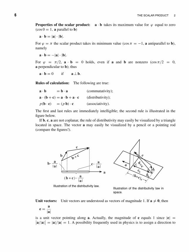
Properties of the scalar product: a · b takes its maximum value for ϕ equal to zero(cos 0 = 1, a parallel to b)
a · b = |a| · |b|.For ϕ = π the scalar product takes its minimum value (cos π = −1, a antiparallel to b),namely
a · b = −|a| · |b|.For ϕ = π/2, a · b = 0 holds, even if a and b are nonzero (cos π/2 = 0,a perpendicular to b); thus
a · b = 0 if a ⊥ b.
Rules of calculation: The following are true:
a · b = b · a (commutativity);
a · (b + c) = a · b + a · c (distributivity);
p(b · c) = (p b) · c (associativity).
The first and last rules are immediately intelligible; the second rule is illustrated in thefigure below.
If b, c, a are not coplanar, the rule of distributivity may easily be visualized by a trianglelocated in space. The vector a may easily be visualized by a pencil or a pointing rod(compare the figures!).
b
a
a
a
a|a | |a |
|a |
c
c.
(b + c ).
b.b + c
Illustration of the distributivity law.
b
( + )b c
a
bc+a
c
caba
Illustration of the distributivity law inspace.
Unit vectors: Unit vectors are understood as vectors of magnitude 1. If a = 0, then
e = a|a|
is a unit vector pointing along a. Actually, the magnitude of e equals 1 since |e| =∣∣a/|a|∣∣ = |a|/|a| = 1. A possibility frequently used in physics is to assign a direction to

THE SCALAR PRODUCT 7
a scalarly formulated equation by the unit vector. For example, the gravitational force hasthe magnitude
F = γmM
r2.
M
mr
er
The unit vector pointingfrom the big mass to thesmall mass is er = r/|r|.
It is acting along the connecting line between the two masses Mand m, hence
F = −γmM
r2
r|r| .
F is the force applied by the mass M to the mass m. Its directionis given by −er = −r/|r|. Hence it is acting toward the mass M .
Cartesian unit vectors: The unit vectors pointing along the positive x-, y-, and z-axesof a Cartesian coordinate frame are defined as follows:
e1 (in x-direction) or also i;
e2 (in y-direction) or also j;
e3 (in z-direction) or also k.
There exist two kinds of Cartesian coordinate frames, namely right-handed frames andleft-handed frames (compare the figures below).
kj
i
right-handed system: k points into the di-rection of a right-handed screw when i → jis rotated along the shortest possible way.
k
j
i
left-handed system: k points into the direc-tion of a left-handed screw when i → j isrotated along the shortest possible way.
We shall always use only right-handed frames in these lectures!
Orthonormality relations: i, j, k or e1, e2, e3 will be used in the following always con-currently, depending on convenience.
We now consider the properties of the Cartesian unit vectors with respect to formation ofscalar products: Since the enclosed angle is each a right one, the following relations hold:
i · i = j · j = k · k = 1 (because of ϕ = 0, hence cos 0 = 1);i · j = i · k = j · k = 0 (because of ϕ = π/2, hence cos π/2 = 0).
(2.1)

8 THE SCALAR PRODUCT 2
These relations are combined by defining
eµ · e = δµ, where δµ =
0 for = µ,
1 for = µ,
and is called the Kronecker symbol.1 For the three-dimensional space, µ and are runningfrom 1 to 3, e1 = i, e2 = j, e3 = k.
1Leopold Kronecker, b. Dec. 7, 1823, Liegnitz (Legnica)—d. Dec. 29, 1891, Berlin. Kronecker was a richprivate person who moved to Berlin in 1855. He taught for many years at the university there, without havinga chair. Only in 1883, after retirement of his teacher and friend Kummer, he took a professorship. His mostimportant publications concern arithmetics, theory of ideals, number theory, and elliptic functions. Kroneckerwas the leading representative of the Berlin School, which claimed the necessity of arithmetization of the entiremathematics.

3 ComponentRepresentationof a Vector
a
c
b
d
f
The vector polygon.
The vector a, which is uniquely represented by the sum ofvectors—in our example by the sum of the vectors b, c, d, f—is called the linear combination of the vectors (e.g., b, c, d,and f). The term “vectors” and their “linear combination” thusgraphically form a closed polygon, the vector polygon. Onemay, of course, conclude from given vectors b, c, d on thelinear combination that yields the arbitrary (but fixed) vector a.
According to the definition introduced above, the vector athen must be a linear combination of the vectors b, c, d;thus
a = q1b + q2c + q3d.
q1, q2, and q3 are denoted as components of the vector a with respect to b, c, d. The vectorsb, c, d must be linearly independent, that is, none of the three vectors may be representedby the other two vectors. Otherwise not every arbitrary vector a could be combined outof the three basic vectors b, c, d. If, for example, d could be expressed by b and c, henced = αb + βc, then a = (q1 + q3α)b + (q2 + q3β)c would always be confined to lie in theplane spanned by b and c. But an arbitrary vector a in general does not lie in this plane(e.g., points out of this plane). One says: The base b, c is incomplete for arbitrary vectorsa. In the three-dimensional space one therefore always needs three basic vectors that arelinearly independent (i.e., cannot be expressed by each other).
Component representation of a vector in Cartesian coordinates: Any vector of thethree-dimensional space may be represented as a linear combination of the Cartesian unit
9

10 COMPONENT REPRESENTATION OF A VECTOR 3
z z′y
y′
x′
x1
11
k j
i
a
azay
ax
The components of a vector are obtained byparallel projection.
vectors i, j, k. This representation leads tosimple and transparent calculations, due tothe orthogonality relations. One then has
a = ax i + ayj + azk,
where ax = a · i, ay = a · j, and az = a · kare the projections of a onto the axes of theframe. The unit vectors i, j, k (or e1, e2, e3)are also called base vectors.
Besides the representation as a sum of vec-tors along the unit vectors, the vector a stillmay be represented as
a = (ax , ay, az) (row notation),
a =
⎛⎜⎜⎝ax
ay
az
⎞⎟⎟⎠ (column notation).
If the base vectors are known, it is sufficient to know the three components.
Calculation of the magnitude of a vector from the components: According to the theo-rem of Pythagoras, the magnitude of a vector a is calculated from its Cartesian componentsas follows:
|a| =√
a2x + a2
y + a2z .
Addition of vectors expressed by components: One has
a + b =3∑
i=1
ai ei +3∑
i=1
bi ei =3∑
i=1
(ai + bi )ei
= (a1 + b1)e1 + (a2 + b2)e2 + (a3 + b3)e3
= (a1 + b1, a2 + b2, a3 + b3) .
Here both commutativity as well as associativity of vector addition have been usedrepeatedly. Thus, the components of the sum vector are the sums of the correspondingcomponents of the individual vectors.
The scalar product in component representation: One has
a · b = (ax i + ayj + azk) · (bx i + byj + bzk),
= ax bx i · i + ax by i · j + ax bz i · k + aybx j · i + aybyj · j + aybzj · k
+ azbx k · i + azbyk · j + azbzk · k .

COMPONENT REPRESENTATION OF A VECTOR 11
Taking into account the orthonormality relations (2.1), we then get
a · b = ax bx + ayby + azbz . (3.1)
Finally, setting for the indices x = 1, for y = 2, and for z = 3, then one can write
a · b =3∑
i=1
ai bi . (3.2)
Hence, the scalar product of two vectors may be evaluated simply by multiplying the cor-responding components of the vectors by each other and summing over the three products.
Problem 3.1: Addition and subtraction of vectors
A DC-10 “flies” north-west at 930 km/h relative to ground. A strong breeze blows from the west with120 km/h relative to ground.
What are the velocity and direction of flight of the plane, assuming that there is no wind deflection?
North
West East
South
y
x
w
vo ey
ex
vm
ϕ
45º
The relative directions of wind and airplane velocity.
Solution Let
|vm | = 930 km/h, the velocity of the plane in the wind,
|v0| = the velocity of the plane without wind,
|w| = the wind velocity.
Now we can write
w = 120 ex ,
vm = −930 cos(45)ex + 930 sin(45)ey
= −657.61ex + 657.61ey,
v0 = vm − w = −777.61ex + 657.61ey
⇒ v0 = |v0| = 1018.39 km/h,
tan ϕ = |v0y ||v0x | = 0.846
⇒ ϕ = 40.2.

12 COMPONENT REPRESENTATION OF A VECTOR 3
z
z
xx
z
x
y
yP (x,y,z)
|r| =
x+
y+
z
22
2
x + y22
r =(x
,y,z
)
The position vector and its coordinates.
The position vector: A point P in space may beuniquely fixed by specifying the vector beginning atthe origin of the coordinate frame and pointing tothe point P as endpoint.
The components of this vector, the position vec-tor, then correspond to the coordinates (x, y, z) ofthe point P . Thus, for the position vector, which ismostly abbreviated by r, there holds
r = x i + yj + zk, or: r = (x, y, z);|r| =
√x2 + y2 + z2.
The angle between two vectors: From the knowl-edge of the two possibilities for represent-ing the scalar product
a · b = |a| |b| cos ϕ = ax bx + ayby + azbz,
one obtains the following relation for the angle enclosed by a and b:
cos ϕ = a · b|a| |b| = ax bx + ayby + azbz√
a2x + a2
y + a2z
√b2
x + b2y + b2
z
.

4 The Vector Product(Axial Vector)
One may define a further product between vectors. Here a new vector arises that is definedas follows.
Definition: The vector product of two vectors a and b is the vector
a × b = (|a| · |b| sin ϕ)n, (4.1)
where n is the unit vector being perpendicular to the plane fixed by a and b, and pointingout of the plane as a right-handed helix when rotating the first vector of the product into
ϕa
b h b= sin ϕ
Geometrical interpretation of theabsolute value of the vector prod-uct as area.
the second vector. Note that the rotation has to be per-formed along the shortest path.
The magnitude of the vector product is equal to the areaof the parallelogram spanned by a and b, as is seen fromthe figure.
F = |a × b| = |a| · |b| sin ϕ = ab sin ϕ,
Properties of the vector product: a × b takes its maximum magnitude for ϕ = π/2,sin(π/2) = 1, a perpendicular to b, |a × b| = |a| |b|.
a × b vanishes for ϕ = 0 (sin 0 = 0, a parallel to b).
a × b = 0
if a ↑↓ b or (↑↓ means antiparallel)
if a ↑↑ b. (↑↑ means parallel)
The formula also includes the special case a = b, thus
a × a = 0.
13

14 THE VECTOR PRODUCT (AXIAL VECTOR) 4
Notations:
represents a vector perpendicular to the drawing plane and pointing out of the plane(arrowhead).
⊗ represents a vector perpendicular to the drawing plane and pointing into the plane(arrowbase).
Rules of calculation: The vector product has the following properties:
I. a × b = −b × a (no commutativity);II. a × (b + c) = a × b + a × c (distributivity);III. a × (b × c) = (a × b) × c (no associativity);IV. p(a × b) = (pa) × b = a × (pb).
(4.2)
Rule I follows immediately from the definition of the vector product (compare with thefigure).
Rule III: The vector on the left side lies in the plane spanned by the vectors b and c; thevector on the right side is in the plane spanned by a and b. The subsequent example alsoshows that associativity does not hold. One has e1 ×(e2 ×e2) = 0, but (e1 ×e2)×e2 = −e1.
Rule II: The proof is given in two steps:
1. Let a be perpendicular (⊥) on b and c, that is, a · b = a · c = 0. Then a × (b + c) =a × b + a × c. The proof for that may be read off immediately from the two figures.a × b stands ⊥ on b and a, is rotated against b by 90, and is longer than b by the factor|a|. The situation is similar for a × c and a × (b + c). The parallelogram of the vectorsa × b, a × c, a × (b + c) emerges from that of the vectors b, c, (b + c) by a rotationabout a by 90 and subsequent stretching by |a|.
ϕ
ϕa b
b a a b= –
11
n
n
a
ab
b
Illustration of the calculational rule I. The direction of rotation is shown.

THE VECTOR PRODUCT (AXIAL VECTOR) 15
a b
a c
b
a
cb c+
ab
c(
+)
Perspective view of the special case: a ⊥ b and a ⊥ c.
a b
ac
b a
cb c+
ab
c
(+
)
Plan view from top of the special case: a ⊥ band a ⊥ c.
b
b
b
c
c c
a
The general case: the vectorsb and c are both decomposedinto components parallel (‖) andperpendicular (⊥) to a.
2. We now decompose in the general case
b = b⊥ + b||,c = c⊥ + c||,
that is, b and c into components ⊥ and || to a (comparewith the figure).
Then, on the one hand, the following holds:
a × b = (|a| · |b| · sin ϕ)a × b|a × b| ;
and, on the other hand,
a × b⊥ = (|a| · |b⊥|) a × b|a × b|
= (|a| · |b| · sin ϕ)a × b|a × b| ,
and therefore
a × b = a × b⊥. (4.3)
This holds for any arbitrary vector b. Therefore, one immediately concludes a × c =a × c⊥. We may then conclude
a × (b + c) = a × (b + c)⊥ = a × (b⊥ + c⊥)
= a × b⊥ + a × c⊥ (because of the special case in 1)
= a × b + a × c (because of (4.3))
q.e.d.

16 THE VECTOR PRODUCT (AXIAL VECTOR) 4
Rule IV: The rule for multiplication by a scalar p is immediately evident if we remindourselves of the meaning of pa.
Vector products of the Cartesian unit vectors: There holds
i × i = j × j = k × k = 0, and i × j = k,
or e1 × e1 = e2 × e2 = e3 × e3 = 0, and e1 × e2 = e3. (4.4)
This product satisfies the cyclic permutability. For an anticyclic permutation one has tomultiply by the factor −1, for example, j × i = −k.
Vector product in components: We now denote the Cartesian unit vectors by e1, e2, e3
instead of i, j, k.Let
a = a1e1 + a2e2 + a3e3 =3∑
i=1
ai ei and b =3∑
i=1
bi ei
be two arbitrary vectors. When forming the vector product of the two vectors a = ∑3i=1 ai ei
and b = ∑3i=1 bi ei , one obtains
a × b = (a1e1 + a2e2 + a3e3) × (b1e1 + b2e2 + b3e3)
= a1b2e3 − a2b1e3 + a2b3e1 − a3b2e1 + a3b1e2 − a1b3e2 (4.5)
= (a2b3 − a3b2)e1 + (a3b1 − a1b3)e2 + (a1b2 − a2b1)e3.
It is now practical to introduce the determinant notation.
Determinants: A rectangular array of numbers is called a matrix (see the figure).
column↓⎛⎜⎜⎜⎝
a11 a12 . . . a1q
a21 a22 . . . a2q
. . . . . . . . . . . .
ap1 ap2 . . . apq
⎞⎟⎟⎟⎠ ← row
For the case q = p, the matrix is called quadratic. One then can assign a numerical valueD to it, called a determinant. It is defined as follows:
I. det(a11) ≡ |a11| = a11;
II. det
(a11 a12
a21 a22
)≡∣∣∣∣∣a11 a12
a21 a22
∣∣∣∣∣ = a11a22 − a12a21; (4.6)

THE VECTOR PRODUCT (AXIAL VECTOR) 17
III. det
⎛⎜⎜⎝a11 a12 a13
a21 a22 a23
a31 a32 a33
⎞⎟⎟⎠ ≡
∣∣∣∣∣∣∣∣a11 a12 a13
a21 a22 a23
a31 a32 a33
∣∣∣∣∣∣∣∣= a11
∣∣∣∣∣a22 a23
a32 a33
∣∣∣∣∣− a12
∣∣∣∣∣a21 a23
a31 a33
∣∣∣∣∣ + a13
∣∣∣∣∣a21 a22
a31 a32
∣∣∣∣∣ .The evaluation of the 3×3 determinants may be simplified by using the so-called Sarrus
rule.1 The procedure is: Establish an additional auxiliary matrix by writing the first twocolumns of the original matrix once again to its right side, and form the product terms,involving signs, according to the following scheme.
a11
a21
a31
a12
a22
a32
a13
a23
a33
a11
a21
a31
a12
a22
a32
+ + +___
Multiple-row determinants may be reduced to determinants of lower order by expansionwith respect to a row or column (formation of subdeterminants), analogous to (eq. (4.6),III). We will see this method at work in Example 4.4 on the Laplace expansion theorem.
Rules of calculation: The most important rules for calculations involving determi-nants are
1. If two rows or columns of the quadratic matrix are identical or proportional to eachother, then the determinant of this matrix = 0.
2. When permuting any two neighboring rows or columns, the sign of the determinantchanges.
3. The determinant of the matrix reflected at the main diagonal (also called the transposedmatrix) is equal to the original determinant.
1Pierre Frederic Sarrus, b. 1798—d. 1861, Saint Affriques. Sarrus was professor of mathematics in Strasbourgfrom 1826 untill 1856. He dealt mainly with the numerical solution of equations with several unknowns (1832),with multiple integrals (1842), and with the determination of comet orbits (1843). The rule for evaluating three-rowdeterminants is named after him.

18 THE VECTOR PRODUCT (AXIAL VECTOR) 4
4. The expansion theorem that has been used in equation (4.6), III, with respect to the firstrow, holds for the first column in the same way.
These rules may easily be checked explicitly in the cases quoted above (eq. (4.6), I, II,III). The cases I –III are the most important ones in the present context. The propertiesof the 3 × 3 determinants will be outlined and discussed in more detail in the context ofProblem 4.3. The rules hold, however, in general for arbitrary determinants.
The vector product (4.5) may now be written as a three-row determinant:
a × b =
∣∣∣∣∣∣∣∣e1 e2 e3
a1 a2 a3
b1 b2 b3
∣∣∣∣∣∣∣∣= e1(a2b3 − a3b2) + e2(a3b1 − a1b3) + e3(a1b2 − a2b1) . (4.7)
If the two vectors of the cross product are equal, then the two lower rows of the determinantare also equal, and the vector product vanishes.
Further, one may easily check based on equation (4.6), III, that the sign of the determinantchanges under permutation of rows (or columns). This corresponds to the anticommutativityof the vector product.
Representation of the product vector: As we already stated in the definition of thevector product, the magnitude of the product vector may be visualized by a distance butbetter by the area of the parallelogram formed by the vectors. This vector is not determinedby its length and orientation only (such vectors are called polar vectors) but is calledan axial vector. To understand this difference, we consider space reflections: We therebychange from the components a1, a2, a3 to the new base vectors a′
1 = −a1, a′2 = −a2,
a′3 = −a3. The vector a is thus reflected at the origin. Under a space reflection, which
is also called a parity transformation, a polar vector changes its sign: a → −a. An axialvector, on the contrary, remains unchanged: a × b = (−a) × (−b).
The invention of these new vectors is necessary since certain physical quantities need ahandedness for a complete description. The handedness is taken into account by an axialvector. Such kinds of quantities are, for instance, the angular velocity and the angularmomentum. One should get straight in one’s mind that a handedness remains unchangedunder a space reflection!
An axial vector may, however, also be represented by an oriented distance.
The double-vector product: The vector product a × (b × c) is called the double-vectorproduct. To evaluate it, we denote the components of b × c as follows: Let
(b × c)x be the x-component,
(b × c)y be the y-component, and
(b × c)z be the z-component.

THE VECTOR PRODUCT (AXIAL VECTOR) 19
For the x-component of the double-vector product, it then follows that
(a × (b × c))x = ay(b × c)z − az(b × c)y
= ay(bx cy − bycx ) − az(bzcx − bx cz).
We add ax bx cx − ax bx cx = 0 and obtain
(a × (b × c))x = bx (ax cx + aycy + azcz) − cx (ax bx + ayby + azbz)
= bx (a · c) − cx (a · b).
Analogous considerations for the y- and z-components of a × (b × c) yield the
Graßmann expansion theorem: One has
a × (b × c) = (a · c)b − (a · b)c,
while
(a × b) × c = (a · c)b − (b · c)a. (4.8)
This is another proof of the fact that the vector product is not associative (see (4.2), III).
Problem 4.1: Vector product
(a) The vector (1, a, b) is perpendicular to the two vectors (4, 3, 0) and (5, 1, 7). Find a and b.
(b) Evaluate in Cartesian coordinates the vector product a × b for a = (1, 7, 0) and b = (1, 1, 1).
(c) Show that
(a × b)2 = a2b2 − (a · b)2 .
Solution (a) It must hold that (1, a, b) · (4, 3, 0) = 0 and (1, a, b) · (5, 1, 7) = 0. This yields the two equations
4 + 3a = 0 and 5 + a + 7b = 0 ⇒ a = −4
3, b = −11
21.
(b)
(a × b)x = (aybz − azby) = 7;(a × b)y = (azbx − ax bz) = −1;(a × b)z = (ax by − aybx ) = −6.
(c)
(a × b)2 = (|a| · |b| · sin ϕ · en)2 = |a|2|b|2 sin2 ϕ(en)
2
= |a|2|b|2(1 − cos2 ϕ)(en)2
= a2b2 − (a · b)2
Here ϕ :<) (a, b) and en is the unit vector along a × b.
20 THE VECTOR PRODUCT (AXIAL VECTOR) 4
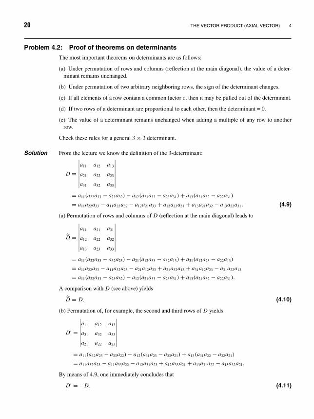
Problem 4.2: Proof of theorems on determinants
The most important theorems on determinants are as follows:
(a) Under permutation of rows and columns (reflection at the main diagonal), the value of a deter-minant remains unchanged.
(b) Under permutation of two arbitrary neighboring rows, the sign of the determinant changes.
(c) If all elements of a row contain a common factor c, then it may be pulled out of the determinant.
(d) If two rows of a determinant are proportional to each other, then the determinant = 0.
(e) The value of a determinant remains unchanged when adding a multiple of any row to anotherrow.
Check these rules for a general 3 × 3 determinant.
Solution From the lecture we know the definition of the 3-determinant:
D =
∣∣∣∣∣∣∣∣a11 a12 a13
a21 a22 a23
a31 a32 a33
∣∣∣∣∣∣∣∣= a11(a22a33 − a23a32) − a12(a21a33 − a23a31) + a13(a21a32 − a22a31)
= a11a22a33 − a11a23a32 − a12a21a33 + a12a23a31 + a13a21a32 − a13a22a31. (4.9)
(a) Permutation of rows and columns of D (reflection at the main diagonal) leads to
D =
∣∣∣∣∣∣∣∣a11 a21 a31
a12 a22 a32
a13 a23 a33
∣∣∣∣∣∣∣∣= a11(a22a33 − a32a23) − a21(a12a33 − a32a13) + a31(a12a23 − a22a13)
= a11a22a33 − a11a32a23 − a21a12a33 + a21a32a13 + a31a12a23 − a31a22a13
= a11(a22a33 − a23a32) − a12(a21a33 − a23a31) + a13(a21a32 − a22a31).
A comparison with D (see above) yields
D = D. (4.10)
(b) Permutation of, for example, the second and third rows of D yields
D′ =
∣∣∣∣∣∣∣∣a11 a12 a13
a31 a32 a33
a21 a22 a23
∣∣∣∣∣∣∣∣= a11(a32a23 − a33a22) − a12(a31a23 − a33a21) + a13(a31a22 − a32a21)
= a11a32a23 − a11a33a22 − a12a31a23 + a12a33a21 + a13a31a22 − a13a32a21.
By means of 4.9, one immediately concludes that
D′ = −D. (4.11)
THE VECTOR PRODUCT (AXIAL VECTOR) 21
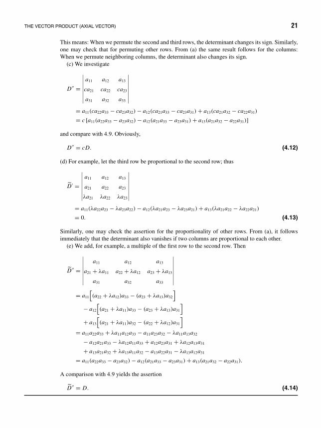
This means: When we permute the second and third rows, the determinant changes its sign. Similarly,one may check that for permuting other rows. From (a) the same result follows for the columns:When we permute neighboring columns, the determinant also changes its sign.
(c) We investigate
D′′ =
∣∣∣∣∣∣∣∣a11 a12 a13
ca21 ca22 ca23
a31 a32 a33
∣∣∣∣∣∣∣∣= a11(ca22a33 − ca23a32) − a12(ca21a33 − ca23a31) + a13(ca21a32 − ca22a31)
= c [a11(a22a33 − a23a32) − a12(a21a33 − a23a31) + a13(a21a32 − a22a31)]
and compare with 4.9. Obviously,
D′′ = cD. (4.12)
(d) For example, let the third row be proportional to the second row; thus
D′ =
∣∣∣∣∣∣∣∣a11 a12 a13
a21 a22 a23
λa21 λa22 λa23
∣∣∣∣∣∣∣∣= a11(λa22a23 − λa23a22) − a12(λa21a23 − λa23a21) + a13(λa21a22 − λa22a21)
= 0. (4.13)
Similarly, one may check the assertion for the proportionality of other rows. From (a), it followsimmediately that the determinant also vanishes if two columns are proportional to each other.
(e) We add, for example, a multiple of the first row to the second row. Then
D′′ =
∣∣∣∣∣∣∣∣a11 a12 a13
a21 + λa11 a22 + λa12 a23 + λa13
a31 a32 a33
∣∣∣∣∣∣∣∣= a11
[(a22 + λa12)a33 − (a23 + λa13)a32
]− a12
[(a21 + λa11)a33 − (a23 + λa13)a31
]+ a13
[(a21 + λa11)a32 − (a22 + λa12)a31
]= a11a22a33 + λa11a12a33 − a11a23a32 − λa11a13a32
− a12a21a33 − λa12a11a33 + a12a23a31 + λa12a13a31
+ a13a21a32 + λa13a11a32 − a13a22a31 − λa13a12a31
= a11(a22a33 − a23a32) − a12(a21a33 − a23a31) + a13(a21a32 − a22a31).
A comparison with 4.9 yields the assertion
D′′ = D. (4.14)

22 THE VECTOR PRODUCT (AXIAL VECTOR) 4
Problem 4.3: Determinants
Calculate using the theorems on determinants:
(a)
∣∣∣∣∣∣∣∣x x + 1 x + 2
0 1 2
3 3 3
∣∣∣∣∣∣∣∣ (b)
∣∣∣∣∣∣∣∣a d xa + yd
b e xb + ye
c f xc + y f
∣∣∣∣∣∣∣∣ (c)
∣∣∣∣∣∣∣∣4 5 22
8 11 44
3 7 1
∣∣∣∣∣∣∣∣Solution (a) We form the linear combination
α · (2. row) + β · (3. row) with α = 1, β = x
3
and obtain (x, x + 1, x + 2), thus just the first row. From (i) and (ii) of (4.6) it follows that thedeterminant is always equal to zero.
(b) The third column is a linear combination of the first and second columns with the factors x and y:
x
⎛⎝ a
b
c
⎞⎠+ y
⎛⎝ d
e
f
⎞⎠ =⎛⎝ xa + yd
xb + yc
xc + y f
⎞⎠ .
From this it follows that the determinant becomes zero.
(c) We expand with respect to the first row:
4
∣∣∣∣∣11 44
7 1
∣∣∣∣∣− 5
∣∣∣∣∣8 44
3 1
∣∣∣∣∣+ 22
∣∣∣∣∣8 11
3 7
∣∣∣∣∣ = 4(−297) − 5(−124) + 22(23) = −62.
Example 4.4: Laplace expansion theorem
Let A = (aik) be a n × n matrix, and Sik be the submatrices of A obtained by erasing the i th row andthe kth column of the matrix A. The matrices Sik thus are (n − 1) × (n − 1) matrices. For each i with1 ≤ i ≤ n, it holds that
det A =n∑
k=1
(−1)i+kaik det Sik (expansion with respect to i th row)
and also
det A =n∑
k=1
(−1)i+kaki det Ski (expansion with respect to i th column).
We check the theorem explicitly for 3-determinants and expand at first the general 3×3 determinant:

THE VECTOR PRODUCT (AXIAL VECTOR) 23
Expansion of det A =
∣∣∣∣∣∣∣∣a11 a12 a13
a21 a22 a23
a31 a32 a33
∣∣∣∣∣∣∣∣ with respect to the first row yields
det A = (−1)1+1a11 S11 + (−1)1+2a12 S12 + (−1)1+3a13 S13 (4.15)
= a11
∣∣∣∣∣a22 a23
a32 a33
∣∣∣∣∣ − a12
∣∣∣∣∣a21 a23
a31 a33
∣∣∣∣∣+ a13
∣∣∣∣∣a21 a22
a31 a32
∣∣∣∣∣ . (4.16)
Expansion of the 3-determinant with respect to the second column yields
det A = (−1)1+2a12 S12 + (−1)2+2a22 S22 + (−1)3+2a32 S32. (4.17)
The first term on the right side is identical with the second term of 4.15. The last two terms of 4.17read explicitly
a22
∣∣∣∣∣a11 a13
a31 a33
∣∣∣∣∣− a32
∣∣∣∣∣a11 a13
a21 a23
∣∣∣∣∣ = a22(a11a33 − a13a31) − a32(a11a23 − a13a21). (4.18)
The sum of the first and third terms of 4.15 or 4.16 yields
a11
∣∣∣∣∣a22 a23
a32 a33
∣∣∣∣∣+ a13
∣∣∣∣∣a21 a22
a31 a32
∣∣∣∣∣ = a11(a22a33 − a23a32) + a13(a21a32 − a22a31). (4.19)
Obviously, 4.18 and 4.19 coincide. Hence, it is clear that the expansions of the 3-determinant withrespect to the first row and the second column, respectively, yield the same. Similarly, one mayverify that the expansion with respect to other rows or columns leads to the same result. Hence, theexpansion theorem for 3-determinants is seen to be valid.
We still evaluate the 3 × 3 determinant by expanding with respect to the second row, and subse-quently with respect to the second column, for the example of the determinant
det A =
∣∣∣∣∣∣∣∣4 5 22
8 11 44
3 7 1
∣∣∣∣∣∣∣∣ .This yields
(a) Expansion with respect to the second row:
det A = (−1)2+1a21 S21 + (−1)2+2a22 S22 + (−1)2+3a23 S23
= −a21
∣∣∣∣∣a12 a13
a32 a33
∣∣∣∣∣+ a22
∣∣∣∣∣a11 a13
a31 a33
∣∣∣∣∣− a23
∣∣∣∣∣a11 a12
a31 a32
∣∣∣∣∣= −8
∣∣∣∣∣5 22
7 1
∣∣∣∣∣+ 11
∣∣∣∣∣4 22
3 1
∣∣∣∣∣− 44
∣∣∣∣∣4 5
3 7
∣∣∣∣∣ = −62. (4.20)

24 THE VECTOR PRODUCT (AXIAL VECTOR) 4
(b) Expansion with respect to the second column:
det A = (−1)2+1a12 S12 + (−1)2+2a22 S22 + (−1)2+3a32 S32
= −a12
∣∣∣∣∣a21 a23
a31 a33
∣∣∣∣∣+ a22
∣∣∣∣∣a11 a13
a31 a33
∣∣∣∣∣− a32
∣∣∣∣∣a11 a13
a21 a23
∣∣∣∣∣= −5
∣∣∣∣∣8 44
3 1
∣∣∣∣∣+ 11
∣∣∣∣∣4 22
3 1
∣∣∣∣∣− 7
∣∣∣∣∣4 22
8 44
∣∣∣∣∣ = −62. (4.21)

5 The Triple ScalarProduct
Definition: The triple scalar product of the three vectors a, b, and c is defined as
a · (b × c) ,
that is, a combination of a scalar and vector product. The triple scalar product is thereforealso denoted as a mixed product. The triple scalar product is a scalar.
Triple scalar product in component representation:
a · (b × c) = (a1, a2, a3) · [(b1, b2, b3) × (c1, c2, c3)]
= (a1, a2, a3) ·
∣∣∣∣∣∣∣∣e1 e2 e3
b1 b2 b3
c1 c2 c3
∣∣∣∣∣∣∣∣= (a1, a2, a3) · (b2c3 − b3c2, −b1c3 + b3c1, b1c2 − b2c1)
= a1(b2c3 − b3c2) − a2(b1c3 − b3c1) + a3(b1c2 − b2c1).
The three terms may again be combined to a determinant, such that
a · (b × c) =
∣∣∣∣∣∣∣∣a1 a2 a3
b1 b2 b3
c1 c2 c3
∣∣∣∣∣∣∣∣ = (a × b) · c. (5.1)
Cyclic permutability: The factors of the triple scalar product may be permuted cyclically.One has
a · (b × c) = b · (c × a) = c · (a × b).
25

26 THE TRIPLE SCALAR PRODUCT 5
These rules may be confirmed easily by successive permutations of the rows in the deter-minant (5.1). The following simplified notation for the triple scalar product may be foundoccasionally in the literature:
a · (b × c) = [a b c ] = [b c a ] = [c a b ].
a
cbγ
ϕ
b c
Illustration of the triple scalar product.
Geometrically, the triple scalar product representsthe volume
V = a · (b × c) = a cos ϕ bc sin γ
= abc cos ϕ sin γ
of a parallelepipedon formed by the three vectors (seefigure).
Note: The volume has a positive sign (+) if alies on the side of b × c, but a negative sign (−) if a lies on the side of −b × c . Hence thevolume might be associated with a sign. In general, however, this choice is not used, and apositive sign is always required. This is achieved by the definition V = |a · (b × c)|.
Properties of the triple scalar product: From
a · (b × c) = 0 follows ϕ = π
2and / or γ = 0, (5.2)
that is, the three vectors are coplanar or (and) two vectors lie on a straight line.This is again a very clear proof of the theorems on determinants already mentioned
above:
1. If two row vectors (or column vectors) are equal or proportional to each other, then thedeterminant equals zero.
2. When we permute two neighboring rows, the determinant changes by a factor (−1).

6 Application of VectorCalculus
Application in mathematics:
Problem 6.1: Distance vectorz
y
x
P1
P2
a
r22 2 2
=( , , )x y z
r 11
11
=(,
,)
xy
z
The distance vector be-tween the points r1 andr2.
Calculate the length of the vector a that represents the distance vectorbetween the points r1 and r2.
Solution a = r2 − r1
= (x2e1 + y2e2 + z2e3) − (x1e1 + y1e2 + z1e3)
= (x2 − x1)e1 + (y2 − y1)e2 + (z2 − z1)e3;hence a reads in row notation
a = (x2 − x1, y2 − y1, z2 − z1),
and the magnitude of a is therefore
|a| = √(x2 − x1)2 + (y2 − y1)2 + (z2 − z1)2 .
Problem 6.2: Projection of a vector onto another vector
a
cec
b
(+
)a
b
The projection of the suma + b onto the vector c.
Given
a = (2, 1, 1),
b = (1, −2, 2),
c = (3, −4, 2),
what is the absolute value of the projection of the sum (a + b) ontothe vector c ?
Solution This projection is given by the scalar product of (a + b) and the unit vector ec along c.
ec = c|c| = (3, −4, 2)√
32 + 42 + 22,
27

28 APPLICATION OF VECTOR CALCULUS 6
(a + b) = (2 + 1, 1 − 2, 1 + 2),
(a + b) · ec = 3 · 3 + (−1) · (−4) + 3 · 2√29
= 19√29
.
Problem 6.3: Equations of a straight line and of a plane
a
xb
X
x
y
A
B
( - )b a
The point-direction form of a straightline.
Let the points A and B be given by their position vectors a andb. What is the equation of the straight line through A and B?
Solution The straight line AB is parallel to (b − a). Moreover, it passesthrough point A. Hence, the equation determining any positionvector x of a point X on the desired straight line reads
x = a + t (b − a),
with t being a real number (running parameter −∞ < t < ∞).If two points A and B are not given but one point A and a vectoru specifying the orientation of the straight line are given, theequation of the straight line reads
x = a + tu .
This is called the point-direction form of the equation of a straight line.
a xE
uv
z
x
y
PP0
t su v+
Representation of a plane in space spannedby the vectors u and v from point P0.
Example:
a = (a1, a2, a3), u = (u1, u2, u3),
x = (a1 + tu1, a2 + tu2, a3 + tu3)
= (x, y, z).
A plane in space may be fixed by specifying be-sides the position vector a and the orientation vectoru still a second orientation vector v:
xE = a + tu + kv,
where u ↑↑— v and also u ↑↓— v and k, t ∈ R. Thenotation ↑↑— and ↑↓— indicates that u and v are neitherparallel nor antiparallel.
This is the point-direction form of the equation ofthe plane.
Example 6.4: The cosine theorem
a
cbγ
The vectors a, b, and ccharacterize the sides ofthe triangle.
The cosine law of plane trigonometry is obtained by scalar multiplicationof the equation c = a − b by itself:
c · c = (a − b) · (a − b) = a 2 + b 2 − 2a · b
= a2 + b2 − 2ab cos γ.
⇒ c2 = a2 + b2 − 2ab cos γ.
For γ = π/2 there results the theorem of Pythagoras.

APPLICATION IN MATHEMATICS 29
Example 6.5: The theorem of Thales
aa
a b+ bb a–
B M A
C
ϑ
The theorem of Thales, demonstratedwith the help of vectors.
In order to prove the theorem of Thales1 we introduce thefollowing vectors according to the sketch:
−→M A = −−→
M B = a,−→MC = b.
It holds that
|a| = |b|, −→BC = a + b, and
−→AC = b − a.
The scalar product (a + b) · (a − b) has the value
(a − b) · (a + b) = a 2 − b 2 = |a|2 − |b|2 = 0.
For the angle enclosed by (a + b) and (a − b), it follows that ϑ = π/2 or
(a + b) ⊥ (a − b) (theorem of Thales).
Example 6.6: The rotation matrix
e2cosβ
e1cosβ
e2sin β
– sine1 β
e2
e1e3
e ′2
e′1
r r= ′
β
β
Case 1: vector r stays at rest; the co-ordinate system is rotated.
The opposite figure shows into which vectors e′1 and e′
2 theCartesian unit vectors e1 and e2 are transformed under arotation in the x, y-plane by the angle β around the z-axis:
e′1 = e1 cos β + e2 sin β + e3 · 0
e′2 = e1(− sin β) + e2 cos β + e3 · 0 (6.1)
e′3 = e1 · 0 + e2 · 0 + e3 · 1 .
This system of equations may be written in matrix form (seeequation 6.7):⎛⎝ e′
1
e′2
e′3
⎞⎠ =⎛⎝ cos β sin β 0
− sin β cos β 0
0 0 1
⎞⎠ ·⎛⎝ e1
e2
e3
⎞⎠
=⎛⎝ d11e1 + d12e2 + d13e3
d21e1 + d22e2 + d23e3
d31e1 + d32e2 + d33e3
⎞⎠ (6.2)
or briefly as
e′ =
3∑µ=1
dµeµ,
1Named after Thales of Milet, b. about 624 BC—d. 546 BC. He is the first representative of the Ionic School.According to writings he did far travels (e.g., to Egypt) and was very active as a politician. The theorem namedafter him was for the first time strictly formulated by him.

30 APPLICATION OF VECTOR CALCULUS 6
where
dµ = e′ · eµ or (dµ) =
⎛⎝ cos β sin β 0
− sin β cos β 0
0 0 1
⎞⎠represent the direction cosines. Note that sin φ = cos(φ − π/2). The matrix (dµ) describes thetransformation of the base vectors. For a rotation in the three-dimensional space in the x, y-plane(i.e., about the z-axis), the rotation matrix reads
D =⎛⎝ cos β sin β 0
− sin β cos β 0
0 0 1
⎞⎠ ≡ (dµ). (6.3)
Case 1: r = r′ fixed in space. If r = r′ is fixed in space but the coordinate frame rotates, one has∑
xe =∑
µ
x ′µe′
µ .
Multiplication of this equation with e′µ isolates x ′
µ:
x ′µ =
∑
x(e · e′µ) =
∑
dµx .
Thus, the transformation of the components of a position vector that is kept fixed in space is given by
r′ = Dr, (6.4)
where D denotes the rotation matrix. Explicitly, this means because of x ′1 = x ′, x ′
2 = y′, x ′3 = z′:
⎛⎝ x ′
y′
z′
⎞⎠new base
=⎛⎝ cos β sin β 0
− sin β cos β 0
0 0 1
⎞⎠ ·⎛⎝ x
y
z
⎞⎠old base
. (6.5)
The addendum “new base” at the column tuple shall indicate that the components x ′, y′, z′ of thecolumn tuple are to be interpreted as coefficients of the base vectors e′
1, e′2, and e′
3. Written explicitly,the vector in the new basis thus reads
r′ = x ′e′1 + y′e′
2 + z′e′3 .
e
e2
e1
e3 3= ′
e′2e′1
r′
rβ
y′
y
x′ xβ
β
Case 2: vector r is rotated togetherwith the coordinate system.
Case 2: r is tightly fixed to the rotating coordinate frame.Thus, r rotates with the coordinate frame. This means∑
xe′ =
∑µ
x ′µeµ
⇒ x ′µ =
∑
x(e′ · eµ)
=∑
dµx
=∑
dµx . (6.6)

APPLICATION IN PHYSICS 31
x ′µ are the new components of the rotated vector with
respect to the fixed system eµ: x are old components ofthe vector with respect to the fixed system eµ.
Note: Both x ′ as well as x in this case are defined in the old system (base eµ). They denote the
components of the new (rotated) and old (not rotated) vector, respectively!In the preceding we have already used the matrix multiplication. It shall once again be clearly
defined here.
Definition of the matrix product: The common element Ci j of the row i and the column j of theproduct matrix C = A · B is obtained by forming the sum
Ci j =∑
k
Aik Bkj , (6.7)
where A and B are the factor matrices.Thus, the components of a vector a = (a1, a2, a3) under rotations of the coordinate frame would
change to⎛⎝ a′1
a′2
a′3
⎞⎠new base
= a′ =⎛⎝ cos β sin β 0
− sin β cos β 0
0 0 1
⎞⎠ ·⎛⎝ a1
a2
a3
⎞⎠
=⎛⎝ cos β a1 + sin β a2
− sin β a1 + cos β a2
a3
⎞⎠ ,
a′µ =
∑
dµa .
The vector itself remains fixed in space. Its components change, however, because the base wasrotated (case 1). If the vector would rotate (case 2), then we would obtain according to 6.6⎛⎝ a′
1
a′2
a′3
⎞⎠new base
=⎛⎝ cos β a1 − sin β a2
sin β a1 + cos β a2
a3
⎞⎠ ; a′µ =
∑
dµa =∑
dµa,
where dµ = dµ is the transposed rotation matrix. The transposed of a matrix is simply the matrixreflected at the main diagonal (from the upper left to the lower right corner).
Application in physics:
Problem 6.7: Superposition of forcesa c
bd20º
30º 45º0 x
110N 100N
80N
160N
Forces acting on point 0.
Four coplanar forces are acting at the point 0, as shownin the sketch.
Calculate the net force acting at the point 0!
Solution a = (−95.3, 55.0) N, b = (−150.4, −54.7) N,

32 APPLICATION OF VECTOR CALCULUS 6
c = (70.7, 70.7) N, d = (80.0, 0.0) N
(N = Newton = 1
kg m
s2
).
It holds that
Fges = a + b + c + d = (−95.0, 71.0) N,
|Fges| =√
95.02 + 71.02 N = 118.6 N.
We remember that
a + b =∑
i
ai ei +∑
i
bi ei =∑
i
(ai + bi )ei = (a1 + b1, a2 + b2, a3 + b3).
βab d
b′ a′
c′c
F =119N
Graphical determination of thenet force F.
Graphical determination of the force: Representation by meansof polygon of forces.
The angle β enclosed by F and the x-axis may be calculatedeasily. One has
F = (−95.0, 71.0) N,Fy
Fx= tan β = −71.0
95.0;
from there it follows that β = 143.
Example 6.8: Equilibrium condition for a rigid body without fixed rotational axis
A rigid body is under the action of the forces Fi at the positions ri . We investigate the equilibrium atthe point A (position vector a) the body may rotate about. All forces Fi are now added and subtractedat A such that nothing is changed in total.
0
B
A
F2 F1
r2r1
r3F3
a
b
A rigid body is in equilibrium with respect topoint A if the sum of all torques with respect toA and the sum of all forces in A vanish. If thiscondition is valid in A, it is also valid in everypoint B.
rF–F
A pair of forces results in a torque M =r × F. These forces set the body onwhich they act into rotation.

APPLICATION IN PHYSICS 33
The procedure is illustrated for the force F1 in the figure on the next page; for the other forceswe proceed in the same way. Now the forces F1 at r1 and −F1 at a are forming a pair of forces thatgenerates the torque (compare with the Problem 6.9)
M1(a) = (r1 − a) × F1 (6.8)
and will rotate the body. Similarly, all other forces Fi (at ri ) and −Fi (at a) are forming pairs of forceswith the torques
Mi (a) = (ri − a) × Fi . (6.9)
The total force acting at the point A is therefore
F =∑
i
Fi , (6.10)
and the total torque about A is
M(a) =∑
i
Mi (a) =∑
i
(ri − a) × Fi . (6.11)
At the point B (position vector b ) a similar construction would yield the total force
F =∑
i
Fi (6.12)
and the total torque about B,
0
1
1
1
1
F
F
r
F
a
b
c b a= –B
A–
Equilibrium with respect to point Aimplies equilibrium with respect topoint B.
M(b) =∑
i
Mi (b) =∑
i
(ri − b) × Fi . (6.13)
The total force F tries to accelerate the body as a whole.The total torque tries to rotate the body. If there shall beequilibrium with respect to point A (position vector a), thenboth the total force F and the total torque M(a) must vanish:
F = 0, (6.14)
M(a) = 0. (6.15)
The question arises of whether an equilibrium at point Aalso means an equilibrium at point B. To answer it, werecalculate the eqs. 6.14, 6.15 to the point B (eqs. 6.12and 6.13). We realize: 6.14 is identical with 6.12. Further, it holds that
M(b) =∑
i
(ri − b) × Fi =∑
i
(ri − (a + c)) × Fi
=∑
i
(ri − a) × Fi −∑
i
c × Fi
= M(a) − c ×∑
i
Fi︸ ︷︷ ︸=0 because of 6.14
= M(a) = 0.
Therefore we may claim: If the equilibrium conditions 6.14,6.15 are fulfilled at a point A, then theyalso hold at any other point B.

34 APPLICATION OF VECTOR CALCULUS 6
Problem 6.9: Force and torque
F2F1
r2
r1
e1
e2e3
Center ofrotation
Rigidbody
Illustration of the torque inducedby two forces.
The following external forces are acting on a body:
F1 = (10, 2, −1) N at point P1(2, 0, 0) cm,
(N = Newton = 1kg m
s2)
F2 = (0, 0, 5) N at point P2(1, 3, 0) cm
andF3 = (−6, 1, 8) N at point P3(6, 8, 1) cm.
Find
(a) components, magnitude, and orientation of the resulting force F,
(b) the torque with respect to P2.
Remark (kp = kilopond). The kilopond is no longer a legal unit, all forces are measured inNewtons (N):
1 N = 1 kg · m
s2= 105 g cm
s2= 105 dyn,
1 kp = 9.81 N.
Solution (a)
F = F1 + F2 + F3 = (4, 3, 12) N,
|F| =√
42 + 32 + 122 N = 13 N,
cos β1 = Fx
|F| = 0.308, β1 = 72,
cos β2 = Fy
|F| = 0.231, β2 = 77,
cos β3 = Fz
|F| = 0.923, β3 = 23.
These are the direction cosines of the force. They describe the direction of force
n = F|F| = (cos β1, cos β2, cos β3) = (0, 308; 0, 231; 0, 923).
r FF′
Center ofrotation
ϑ
The absolute value of the torque results fromthe force component perpendicular to the dis-tance vector.
(b) The torque of a force Fp acting at pointP(x, y, z), that is at the position r = (x, y, z), isdefined with respect to the coordinate origin (centerof rotation) as the vector
M = r × Fp.
Here r is the position vector from the cen-ter of rotation to the action point of the forceFp . The magnitude of M is obviously given by

APPLICATION IN PHYSICS 35
M = r · F ′, where F ′ = F sin ϑ is the force component perpendicular to the position vector (comparein the figure). This may also be expressed as follows: M = distance from center of rotation to actionpoint of the force times force component perpendicular to the distance vector.
r–F
F
FCenter ofrotation
The pair of forces responsible for thetorque.
This torque M is also caused by a pair of forces, asdiscussed in Example 6.8. If one adds at the center ofrotation the forces −F and F, in total 0 (compare to thefigure), then the forces −F at the center of rotation and Fat r form a pair of forces. The force F acting at the centerof rotation presses onto the bearing of the rotation axis andis received there.
If several forces F are acting on the rigid body atthe points r, the total torque is
M =∑
M =∑
r × F.
In our example
M = (r1 × F1) + (r2 × F2) + (r3 × F3),
r1 = p1 − p2 = (1, −3, 0) cm,
r2 = p2 − p2 = (0, 0, 0) cm,
r3 = p3 − p2 = (5, 5, 1) cm,
where p1, p2, and p3 are the position vectors of the points P1, P2, and P3. Hence one obtains
M1 = r1 × F1 = (3, 1, 32) N cm,
M2 = r2 × F2 = 0 N cm,
M3 = r3 × F3 = (39, −46, 35) N cm.
The total torque is
M = M1 + M2 + M3 = (42, −45, 67) N cm,
and |M| = 91.0 N cm.
Problem 6.10: Forces in a three-leg stand
Find the rod forces in a three-leg stand that is movably linked at the points A, B, C to a vertical walland loaded at the point D by the force F.
Solution Only longitudinal forces may act in the rods, because of the movable links of the suspension rods(neglect of bending forces). The forces at the cut-out branching point D are to be considered asexternal forces and are obtained from the equilibrium condition
F1 + F2 + F3 + F = 0. (6.16)
Using the unit vectors ei (i = 1, 2, 3) along the rod axes and the magnitudes Fi (i = 1, 2, 3) ofthe rod forces, 6.16 may be written as
F1e1 + F2e2 + F3e3 = −F. (6.17)
To get the rod forces, 6.17 is scalar-multiplied successively by the vectors ei × ej (i = j), where(ei × ej ) by definition points perpendicular to ei , hence the scalar products ei · (ei × ej ) vanish.

36 APPLICATION OF VECTOR CALCULUS 6
Using the definition of the triple scalar product A · (B × C), one then obtains from 6.17 for Fi
(i = 1, 2, 3)
F1 = − F · (e2 × e3)
e1 · (e2 × e3), F2 = − F · (e3 × e1)
e2 · (e3 × e1), F3 = − F · (e1 × e2)
e3 · (e1 × e2). (6.18)
Putting a coordinate frame into the branching point D according to the above figure, one gets forthe unit vectors
e1 = (− cos α, sin α, 0),
e2 = (cos α, sin α, 0), (6.19)
e3 = (0, sin β, − cos β).
Insertion of equation 6.19 into equation 6.18 yields
F · (e2 × e3) =
∣∣∣∣∣∣∣∣Fx Fy Fz
cos α sin α 0
0 sin β − cos β
∣∣∣∣∣∣∣∣ (6.20)
= −Fx sin α cos β + Fy cos α cos β + Fz cos α sin β
and
e1 · (e2 × e3) =
∣∣∣∣∣∣∣∣− cos α sin α 0
cos α sin α 0
0 sin β − cos β
∣∣∣∣∣∣∣∣ (6.21)
= 2 sin α cos α cos β.
From there one obtains for the component F1
F1 = 1
2
(Fx
cos α− Fy
sin α− Fz tan β
sin α
). (6.22)
Fz
xy
D
BA
Cβ
αα
A three-leg stand fixed at a vertical wall.
F2
F
F1
F3
z
xy
D
The forces acting at the three-legstand.

APPLICATION IN PHYSICS 37
The calculation of the scalar triple products for F2 and F3 from equation 6.18 runs in an analogousmanner; one gets
F2 = 1
2
(− Fx
cos α− Fy
sin α− Fz tan β
sin α
), (6.23)
F3 = Fz
cos β.
Problem 6.11: Total force and torque
(a) Determine the components Fy , Fz of the force F = (2 N, Fy, Fz) acting at point P1(1, 2, 3) m suchthat it is perpendicular to the plane defined by the three points P1, P2(2, 3, 4) m, and P3(2, 2, 1) m.
(b) What is the magnitude of the force F and which torque M does it apply with respect to the pointP4(0, 1, 2) m?
(c) What is the component of the torque vector M that points perpendicular to the plane?
r2
r4r 3
r 1
z
x
y
P1
P4
P2
P3
Fr
r14
–
rr
13
- rr1
2-
The force F acting at P1 applies a torque around P4.
Solution (a) Because the vectors (r1 − r2) and (r1 − r3) are within the represented plane, the vector productR = (r1 − r2) × (r1 − r3) yields a normal vector R perpendicular to the plane. If the force F shall beperpendicular to the plane, that is, parallel to the vector R, the following must hold:
R = (Rx , Ry, Rz) = (r1 − r2) × (r1 − r3) = λF = λ (2 N, Fy, Fz). (6.24)
From there it follows that
λ = 1
2 NRx , Fy = 1
λRy , Fz = 1
λRz . (6.25)
For the points P1(1, 2, 3) m, P2(2, 3, 4) m, P3(2, 2, 1) m, and P4(0, 1, 2) m specified in the problem,one easily gets the position vectors ri (i = 1, 2, 3, 4) as well as their differences (ri − rj ) (i = j):
(r1 − r2) = (−1, −1, −1) m,
(r1 − r3) = (−1, 0, 2) m, (6.26)
(r1 − r4) = (1, 1, 1) m.

38 APPLICATION OF VECTOR CALCULUS 6
For the vector product in equation 6.24, it then results that
R = (r1 − r2) × (r1 − r3) = (−2, 3, −1) m2 = (Rx , Ry, Rz).
Inserting these values in 6.25, one obtains
λ = 1
2 NRx = −1 m2N−1,
Fy = Ry
λ= −3 N, (6.27)
Fz = Rz
λ= 1 N.
Thus, the components of the force F are
F = (2, −3, 1) N. (6.28)
(b) The magnitude of the force F is obtained as
|F| = (F2x + F2
y + F2z )1/2 = (22 + 32 + 1)1/2 N ≈ 3.74 N. (6.29)
The torque M with respect to the point P4 results from the vector product
M = (r1 − r4) × F = (1, 1, 1) × (2, −3, 1)Nm = (4, 1, −5) Nm. (6.30)
(c) The component of the torque vector M perpendicular to the plane, that is, along the orientation ofthe force F, results from the definition of the triple scalar product as
|MF| = [(r1 − r4) × F ] · F|F| = 0. (6.31)

7 Differentiationand Integrationof Vectors
Formation of the differential quotient: The vector A may occur as a function of aparameter. Let’s consider, for example, the position vector r(t) that—as a function of thetime t—describes the path of a mass point. If one decomposes A into its components withrespect to fixed unit vectors, then these components are functions of the parameter. Wewrite
A(u) = Ax (u)e1 + Ay(u)e2 + Az(u)e3. (7.1)
The differential quotient of a vector is formed by differentiating its components sepa-rately, as corresponds to the differentiation rule for sums. Because the unit vectors are notvariables, they are conserved under differentiation,
dA(u)
du= lim
u→0
A(u + u) − A(u)
u
= limu→0
(Ax (u + u) − Ax (u)
ue1 + Ay(u + u) − Ay(u)
ue2
+ Az(u + u) − Az(u)
ue3
).
The limit of the sum is equal to the sum of the limits, that is, when passing to the limit,one obtains
dA(u)
du= d Ax (u)
due1 + d Ay(u)
due2 + d Az(u)
due3. (7.2)
39

40 DIFFERENTIATION AND INTEGRATION OF VECTORS 7
By comparing (7.1) with (7.2), one notices that the differentiation of a vector in anarbitrary coordinate frame with fixed unit vectors amounts to the differentiation of thecomponents of the vector. Generally, the rule for the n-fold differentiation of a vector reads
dnA(u)
dun= dn Ax (u)
dune1 + dn Ay(u)
dune2 + dn Az(u)
dune3. (7.3)
Example 7.1: Differentiation of a vector
A(u) = (2u2 − 3u)︸ ︷︷ ︸Ax (u)
e1 + (5 · cos u)︸ ︷︷ ︸Ay (u)
e2 − (3 · sin u)︸ ︷︷ ︸Az (u)
e3,
= (2u2 − 3u, 5 · cos u, −3 · sin u),
dA(u)
du= (4u − 3)e1 − (5 · sin u)e2 − (3 · cos u)e3
= (4u − 3, −5 · sin u, −3 · cos u),
d2A(u)
du2= 4e1 − 5 · cos u · e2 + 3 · sin u · e3
= (4, −5 · cos u, 3 · sin u).
For composite functions the usual differentiation rules apply. For example, for the productof a scalar function and a vector function, or for the scalar or vector product of two vectorfunctions (parameter u), the product rule applies.
Differentiation of the product of a scalar and a vector:
d(φ(u)A(u))
du= d
du(φ(u)Ax (u)e1 + φ(u)Ay(u)e2 + φ(u)Az(u)e3) .
Now
d(φ Ax )
du= dφ
duAx + φ
d Ax
du
and analogously for the other components:
d
du(φ Ai ) = d
du(φ)Ai + d
du(Ai )φ (i = 1, 2, 3).
This yields
d(φ(u) · A(u))
du= dφ
duAx e1 + dφ
duAye2 + dφ
duAze3 + φ
d Ax
due1 + φ
d Ay
due2 + φ
d Az
due3
or simply
d(φ(u)A(u))
du= dφ
duA + φ
dAdu
. (7.4)

DIFFERENTIATION AND INTEGRATION OF VECTORS 41
Differentiation of the scalar product: One has
d(A(u) · B(u))
du= d
du
(3∑
i=1
Ai (u)Bi (u)
)=
3∑i=1
d
du(Ai (u)Bi (u))
=3∑
i=1
(d Ai (u)
duBi (u) + Ai (u)
d Bi (u)
du
)and therefore,
d(A(u) · B(u))
du= dA
du· B + A · dB
du. (7.5)
Differentiation of the vector product: It is performed analogously to the differentiationof the scalar product. Because the vector product is not commutative, one has to take careof the ordering of the factors.
d
du(A(u) × B(u)) = dA(u)
du× B(u) + A(u) × dB(u)
du. (7.6)
This is easily proved by checking the individual components (e.g., the x-component) onboth sides of the equation.
Example 7.2: Differentiation of the product of a scalar and a vector
For the scalar function ϕ(x) = x + 5 and the vector function A(x) = (x2 + 2x + 1, 2x, x + 2) thesecond derivative of the products ϕ · A is to be calculated.
The differentiation of the product yields
d2(ϕA)
dx2= d
dx
(dϕ
dxA + ϕ
dAdx
)= d2ϕ
dx2A + 2
dϕ
dx
dAdx
+ ϕd2Adx2
.
The derivatives of the individual functions read
dϕ
dx= 1,
d2ϕ
dx2= 0,
dAdx
= (2x + 2, 2, 1),d2Adx2
= (2, 0, 0).
From the above, it results that
d2(ϕA)
dx2= (4x + 4, 4, 2) + (2x + 10, 0, 0) = (6x + 14, 4, 2).
Application: Position, velocity, and acceleration of a mass point on a defined trajectorymay be represented as vectors. The position vector for the motion of the mass point onan arbitrary trajectory B is the vector from the origin of the coordinate frame to the masspoint; the variation of the position of the mass point with the time may be represented astime variation of the position vector (compare with the figure).

42 DIFFERENTIATION AND INTEGRATION OF VECTORS 7
z
y
x
B
r( )t
r(+
)t
t∆
∆ ∆r r r= ( + )– ( )t t t
Definition of the orbital velocity: r = r(t + t) − r(t) is a secant vector to the orbit at the point r(t). Thevelocity is then given by v = limt→0 r/t .
The velocity is defined as the first derivative of the position vector r(t) of the orbitalcurve with respect to the time:
v = limt→0
rt
= limt→0
r(t + t) − r(t)t
= drdt
. (7.7)
From equation (7.7) one notices that the vector of the velocity represents the limit positionof the secant through the position vectors r(t + t) and r(t) divided by the time intervalt in the limit t → 0, that is, the velocity points along the tangent to the trajectory at thepoint r(t).
The acceleration is obtained as the first derivative of the velocity with respect to the time,or as the second derivative of the position vector with respect to the time:
a(t) = dv(t)
dt= lim
t→0
vt
= d(dr /dt)
dt= d2r(t)
dt2. (7.8)
Because the position vector is a vector, its derivatives with respect to the scalar time (t)are again vectors. Thus, the velocity and acceleration are vectors, too.
Problem 7.3: Velocity and acceleration on a space curve
Let the position vector be given by r = (t3 + 2t, −3e−t , t) m. Find the velocity and the accelerationas well as their magnitudes for the time points t = 0 s and t = 1 s.
Solution For the velocity and acceleration, we get
v(t) = r = (3t2 + 2, 3e−t , 1)m
s,
a(t) = r = (6t, −3e−t , 0)m
s2.
For the time t = 0, the results are
v(0) = (2, 3, 1)m
s, a(0) = (0, −3, 0)
m
s2,

DIFFERENTIATION AND INTEGRATION OF VECTORS 43
v(0) = √14
m
s, a(0) = 3
m
s2.
For t = 1 s,
v(1) = (5,3
e, 1)
m
s, a(1) = (6, −3
e, 0)
m
s2,
v(1) = 5.22m
s, a(1) = 6.1
m
s2.
Example 7.4: Circular motion
The Cartesian components of a circular motion are given by
x(t) = R cos ωt,
y(t) = R sin ωt,
z(t) = 0.
ω is the so-called angular velocity or also angular frequency. It is related to the revolution period T
x t( )
y t( )
xR
y
ωt
v
r()t
Circular motion.
via ωT = 2π . The position vector is now
r(t) = (x(t), y(t), z(t))
= x(t)e1 + y(t)e2 + z(t)e3,
r(t) = (R · cos ωt, R · sin ωt, 0)
= R · cos ωt e1 + R · sin ωt e2 + 0e3.
For the velocity one gets
v = drdt
= (−ωR · sin ωt, Rω cos ωt, 0).
There holds
r · v = r · drdt
= 0 for any time point,
⇒ v ⊥ r,
which is immediately clear for a circular orbit.For the magnitude of the velocity, one obtains
v = |v| =√(
dx
dt
)2
+(
dy
dt
)2
+(
dz
dt
)2
=√
ω2 R2 sin2 ωt + ω2 R2 cos2 ωt + 0
=√
ω2 R2(sin2 ωt + cos2 ωt) = ωR = 2π R
T= circumference
revolution period.
The acceleration is obtained as
b = dvdt
= d2rdt2
= (−ω2 R cos ωt, −ω2 R sin ωt, 0) = −ω2(R cos ωt, R sin ωt, 0),
= −ω2r.

44 DIFFERENTIATION AND INTEGRATION OF VECTORS 7
It turns out that the acceleration points opposite the orientation of the position vector (centripetalacceleration). The magnitude of the acceleration is given by
|b| =√(
d2x
dt2
)2
+(
d2 y
dt2
)2
+(
d2z
dt2
)2
,
= ω2 R = v2
R.
Example 7.5: The motion on a helix
x
Pitch= 2h b . π
z
y
The helix and its pitch.
The Cartesian coordinates of the helix read
x(t) = R cos ωt, y(t) = R sin ωt, z(t) = bωt.
The position vector is obtained by insert-ing in the relation
r(t) = (x(t), y(t), z(t)) ,
that is, it holds that
r(t) = (R cos ωt, R sin ωt, bωt).
Remark: b > 0 means right-handed he-lix, b < 0 means left-handed helix.
The velocity results analogously to thatof circular motion
v = (−Rω sin ωt, Rω cos ωt, bω).
The third component v3 = bω implies a uniform (constant) upward velocity (z-direction) if theparameter t represents the time.
One has
|v| =√
R2ω2 + b2ω2 = ω√
R2 + b2,
that is, the magnitude of the velocity is constant.The acceleration is the derivative of the velocity
b = −ω2 · (R cos ωt, R sin ωt, 0) = −ω2r⊥,
wherer⊥ = (R cos ωt, R sin ωt, 0) = (r · er )er
and er = (cos ωt, sin ωt, 0) is the polar unit vector in the x, y-plane. We thus obtain the sameacceleration as for the circular motion. For the magnitude, it holds that |b| = ω2 R.
Integration of vectors: The integration rules may be applied also to vectors in thecustomary way. For a vector A depending on a parameter (e.g., u), it follows that∫
A(u) du =∫ (
Ax (u)e1 + Ay(u)e2 + Az(u)e3)
du

DIFFERENTIATION AND INTEGRATION OF VECTORS 45
=∫
Ax (u) e1 du +∫
Ay(u) e2 du +∫
Az(u) e3 du.
If the unit vectors are constant, they may be pulled out before the integral symbol:∫A(u) du = e1
∫Ax (u) du + e2
∫Ay(u) du + e3
∫Az(u) du.
Thus, we may formulate the following rule: A vector is integrated by integrating itscomponents. This vector integration graphically means a summation of a large number ofvectors according to the integral limits; for example, the sum of all forces acting on a body.More strictly speaking: A(u) is a vector density, and dA = A(u) du is the vector associatedwith the interval du. These dA are summed to yield the integral. An example is the impulseof force K, which is understood as the force K acting on a body over a time interval; thusK = ∫
t F(t ′) dt ′. The impulse of force is therefore the sum of the forces F(t ′) actingduring the time interval. For more details, see Chapter 17, equations (17.14) and (17.15).
Example 7.6: Integration of a vector
A = (2u2 − 3u, 5 cos u, −3 sin u),∫A du =
(2
3u3 − 3
2u2 + C1
)e1 + (5 sin u + C2)e2 + (3 cos u + C3)e3
=(
2
3u3 − 3
2u2
)e1 + (5 sin u)e2 + (3 cos u)e3 + C1e1 + C2e2 + C3e3
=(
2
3u3 − 3
2u2, 5 sin u, 3 cos u
)+ C.
The integration constants arising in the components are composed to the vector C.
Problem 7.7: Integration of a vector
Calculate
2∫0
A(n) dn with A = (3n2 − 1, 2n − 3, 6n2 − 4n).
Solution∫ 2
0A(n) dn =
∫ 2
0(3n2 − 1, 2n − 3, 6n2 − 4n) dn
= [(n3 − n, n2 − 3n, 2n3 − 2n2)
]2
0
= (6, −2, 8).

46 DIFFERENTIATION AND INTEGRATION OF VECTORS 7
Problem 7.8: Motion on a special space curve
(a) Which curve is passed by the vector
r(t) = (x(t), y(t), z(t)) = (t cos t, t sin t, t)
when t is running from 0 to 2π?
(b) Calculate the velocity and acceleration of the point at the time t .
(c) What are the velocity and acceleration for t = 0 and t = 2?
(d) How do the magnitudes of radius vector, velocity, and acceleration vary for large time t?
y
x
t = 0
t = 2π
2π
r ( )t~
The resulting spiral line with a radiusvarying from 0 to 2π .
Solution (a) We first consider the vector r (t) with z(t) ≡ 0(projection onto the x, y-plane).
r (t) = (t cos t, t sin t, 0).
Because
|r (t)| = (t2 cos2 t + t2 sin2 t)1/2 = t,
there results a spiral line with a radius from 0 to 2π .If z(t) = t additionally runs from 0 to 2π , we obtain
a spiral line on the surface of a cone of height 2π withthe vortex at (0, 0, 0).
The figure at the top of the facing page illustrates thisresult.
(b) For the velocity v(t) and acceleration b(t), it re-sults that
v(t) = drdt
= (cos t − t sin t, sin t + t cos t, 1),
b(t) = dvdt
= d2rdt2
= (− sin t − sin t − t cos t, cos t + cos t − t sin t, 0),
= (−2 sin t − t cos t, 2 cos t − t sin t, 0),
(c) One has
v(t = 0) = (1, 0, 1); |v(t = 0)| = √2 ,
v(t = 2) = (−2.23, 0.08, 1); |v(t = 2)| = √6 ,
b(t = 0) = (0, 2, 0); |b(t = 0)| = 2 ,
b(t = 2) = (−0.99, −2.65, 0); |b(t = 2)| = √8 .
(d)
|r(t)| = (t2 cos2 t + t2 sin2 t + t2
)1/2 = √2 |t |,
|v(t)| = ((cos t − t sin t)2 + (sin t + t cos t)2 + 1
)1/2

DIFFERENTIATION AND INTEGRATION OF VECTORS 47
t = 2π
2π
r ( )tt = 0
x
y
z
The spiral line on the surface of a cone.
= (2 + t2)1/2 = |t |(
1 + 2
t2
)1/2
= |t |
1 + 1
t2− O
(1
t4
)t1−→ |t | (by a series expansion of the square root),
|b(t)| = ((2 sin t + t cos t)2 + (2 cos t − t sin t)2
)1/2
= (4 + t2)1/2 = |t |(
1 + 4
t2
)1/2
= |t |
1 + 2
t2− O
(1
t4
)t1−→ |t | (by a series expansion of the square root).
Problem 7.9: Airplane landing along a special space curve
An airplane is landing. Thereby it is moving on the space curve
r(t) = (x(t), y(t), z(t)) = (R cos ωt, R sin ωt, (H − bωt)),
with
R = 1000 m,
ω = 1
7s−1,
H = 400 m,
b = H/6π,
t ∈ [0, 42π ] s.

48 DIFFERENTIATION AND INTEGRATION OF VECTORS 7
What is the velocity of the plane on landing (at t = 42π s)? Would you try landing this way?
Solution The velocity is calculated to be
v = drdt
= (−ωR sin ωt, ωR cos ωt, −bω),
and its magnitude is
|v| = (ω2 R2 sin2 ωt + ω2 R2 cos2 ωt + b2ω2)1/2
= ω(R2 + b2)1/2 .
Obviously, it is independent of t! Insertion of the values yields
|v| = 1
7
(10002 + 4002
(6π)2
)1/2
m s−1
≈ 142.9 m s−1 = 514.4 km h−1 .
This kind of landing is certainly unsuitable; the approach velocity should better be reduced.

8 The Moving Trihedral(AccompanyingDreibein)—theFrenet Formulas
In some cases it may be simpler to express velocity and acceleration in natural coordinates.This means that the velocity and acceleration are not derived from the variation of theposition vector with the time, but from its variation with the passed way s, the arc length,the starting point being arbitrary. Let the curve itself be given by the position vectorr(t) = (x1(t), x2(t), x3(t)). For infinitesimally small segments, the increase of the arclength is |dr| = ds.
0
∆s
∆r
r( )tr( + )t t∆
In the limit of small t , theabsolute value of the secantvector r becomes the lineelement ds, that is, |r| →ds.
The arc length s of the curve between the parameter valuest0 and t is then obtained by integration:
s(t) =∫ t
t0
ds =∫ t
t0
|dr| =∫ t
t0
|dr|dt
dt (8.1)
=∫ t
t0
√(dx1
dt
)2
+(
dx2
dt
)2
+(
dx3
dt
)2
dt.
The magnitude of the velocity is
|v| =∣∣∣∣drdt
∣∣∣∣ = |dr|dt
= ds
dt.
In order to become independent of the coordinate frame, a set of orthogonal unit vectorsis put at the point of the trajectory of the mass point given by s. The set of unit vectorsmoves along with the mass point: it is therefore also called the “moving trihedral” or“accompanying dreibein.” As unit vectors one uses
49

50 THE MOVING TRIHEDRAL (ACCOMPANYING DREIBEIN)—THE FRENET FORMULAS 8
T tangent vector,
N principal normal vector,
B binormal vector.
Because the vectors form an orthonormalized set, it holds that (N × B) = T, cyclicallypermutable. In the following we give the precise definition of these three base vectors ofthe moving trihedral and show how they are calculated for a given space curve r(t).
The function r(t) describes a space curve depending on the time t as a parameter. Todetermine the moving trihedral, one has to convert the function r(t) into r(s); this is doneby substituting the time t = t (s) from s = s(t) (compare with equation (8.1)).
The moving trihedral is determined from the local properties of the trajectory. dr /ds isa vector along the limit position of the secant, i.e., the tangent.
z
y
x
Ps
N
B
T( )t r( )t
∆T N~
T( + )t t∆
s0
A curve in space and the moving trihedral (shown at an arbitrary point P of the curve).
The magnitude of this vector is |r|/s. For infinitesimally small segments one has|dr| = ds; thus |dr|/ds = 1. Hence one has determined the tangent unit vector:
T = drds
.

THE MOVING TRIHEDRAL (ACCOMPANYING DREIBEIN)—THE FRENET FORMULAS 51
T( )s
T( )s
∆T
T( + )s s∆s s+∆
s
The difference vector T is a measure of thecurvature of the curve. T points toward the“inner side” of the curve. A straight line hasno curvature, and the normal vector N is notuniquely defined.
Because ds = |dr|, it also holds that
T = dr|dr| = dr / dt
|dr / dt | = v|v| .
In order to determine the principal normalvector, one first forms
T · T = 1.
By differentiating the scalar product of the tan-gent vector, one obtains
d
ds(T · T) = dT
ds· T + T · dT
ds= 0.
Because the commutative law holds for the scalar product, T·dT/ds is zero. This impliesthat dT /ds is perpendicular to T.
The vector dT /ds gives the orientation of the principal normal vector. We characterizeits position by constructing, besides the tangent defined by T(s), a second tangent T(s+s)(neighboring tangent) that differs from the first one only by an infinitesimal vector T (seefigure). The principal normal vector lies in the plane spanned by the two tangents T(s) andT(s + s). Because the magnitude of dT /ds in general differs from unity, one still has tointroduce a factor κ for normalization:
κ · N = dTds
,
where κ = |dT/ds|. This is the first Frenet formula. The value κ is always defined aspositive. This is possible since the orientation of N may be chosen in an appropriatemanner. The factor κ is called the curvature of the space curve.
The third unit vector, the binormal vector, is formed out of T and N:
B = T × N.
The orientations of all three unit vectors are functions of the arc length.The vectors of the moving trihedral (accompanying dreibein) may be differentiated with
respect to the arc length. The three differential quotients are called Frenet’s1 formulas andread
dTds
= κN, (8.2)
dNds
= τB − κT, (8.3)
1Jean Frederic Frenet, b. Feb. 7, 1816—d. June 12, 1900, Perigueux (Dordogne). In 1840 Frenet enteredthe Ecole Normale in Paris as a scholar, was appointed as professor in 1848, and taught until 1868 at LyonUniversity. His research mainly concerned problems of differential geometry, and in 1847 he found the Frenetforms independently of Serret.

52 THE MOVING TRIHEDRAL (ACCOMPANYING DREIBEIN)—THE FRENET FORMULAS 8
dBds
= −τN or |τ | =∣∣∣∣dB
ds
∣∣∣∣ . (8.4)
τ is a conversion factor and is called the torsion. The torsion describes the winding of thecurve out of the T, N-plane. The quantity dB/ds is exactly a measure for this winding.From the curvature and torsion one gets
= 1
κcurvature radius, σ = 1
τtorsion radius.
The curvature radius of a curve at a definite point equals the radius of the osculatingcircle having the same curvature as the curve at that point.
Formula (8.2) has already been introduced as a definition. For a transparent derivationof the remaining formulas, one utilizes the statement that any vector may be represented asa linear combination of the three unit vectors.
Derivation of the second Frenet formula: Because the moving trihedral spans the entirethree-dimensional space, it holds that
dNds
= αT + βN + γ B ,
where α, β, γ are to be determined. Because N is a unit vector, N · N = 1.By differentiating the scalar product N · N, one obtains
d
ds(N · N) = d
ds(1) = 0
or in other notation (product rule) dN/ds ·N+N ·dN/ds = 0, or, because the commutativelaw holds for the scalar product:
2N · dNds
= 0.
Because in the nontrivial case neither N nor dN /ds is equal to zero, this means thatdN /ds is perpendicular to N, i.e., there is no component of dN /ds along N. Therefore,
β = 0; i.e.,dNds
= αT + γ B. (8.5)
Moreover, according to the definition of the unit vectors, T · N = 0. By forming the firstderivative of this scalar product one has
dTds
· N + T · dNds
= 0. (8.6)
Using the first Frenet formula, we find
dTds
· N = κN · N = κ. (8.7)

THE MOVING TRIHEDRAL (ACCOMPANYING DREIBEIN)—THE FRENET FORMULAS 53
By inserting (8.7) in (8.6), we obtain
κ + T · dNds
= 0, or T · dNds
= −κ.
Multiplication of equation (8.5) by T yields
T · dNds
= αT · T + γ B · T = α.
Because T · dN/ds = −κ , it follows that α = −κ . Hence
dNds
= −κT + τB,
where γ = τ is defined and inserted as conversion factor.
Derivation of the third Frenet formula: We first try with the preceding trick and startfrom B · N = 0. If we differentiate the scalar product B · N, the product rule yields
dBds
· N + B · dNds
= 0.
But this does not help immediately. We therefore simply start from the definition of B.Because B = T × N, it follows that
dBds
= d
ds(T × N) = dT
ds× N + T × dN
ds. (8.8)
The first term of the equation may be transformed as follows:
dTds
× N = κN × N = 0. (8.9)
By inserting equation (8.9) in (8.8), it follows that
dBds
= T × dNds
.
With
dNds
= τB − κT,
it follows that
dBds
= T × (τB − κT),dBds
= τ(T × B) − κ(T × T).
Because
T × B = −N and T × T = 0 ,
it follows that
dBds
= −τN.
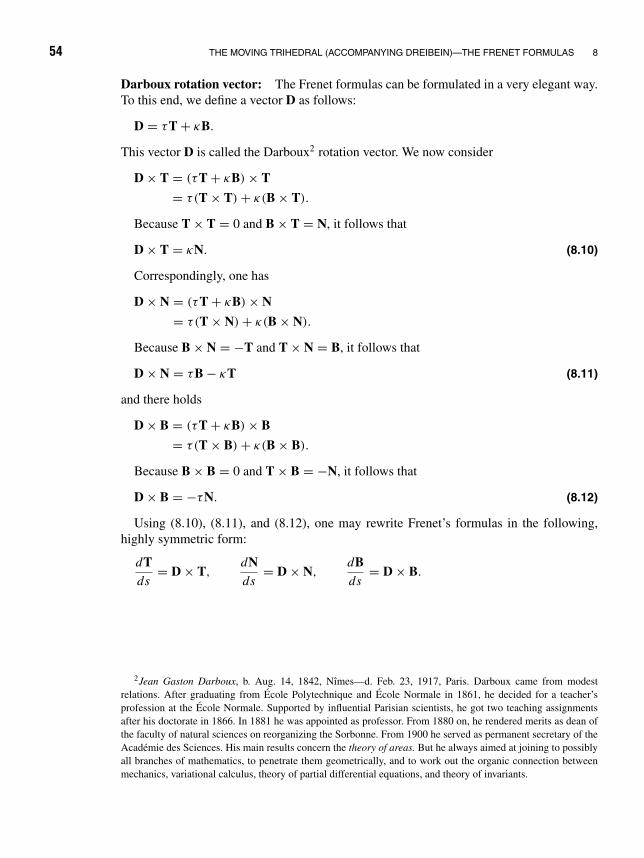
54 THE MOVING TRIHEDRAL (ACCOMPANYING DREIBEIN)—THE FRENET FORMULAS 8
Darboux rotation vector: The Frenet formulas can be formulated in a very elegant way.To this end, we define a vector D as follows:
D = τT + κB.
This vector D is called the Darboux2 rotation vector. We now consider
D × T = (τT + κB) × T
= τ(T × T) + κ(B × T).
Because T × T = 0 and B × T = N, it follows that
D × T = κN. (8.10)
Correspondingly, one has
D × N = (τT + κB) × N
= τ(T × N) + κ(B × N).
Because B × N = −T and T × N = B, it follows that
D × N = τB − κT (8.11)
and there holds
D × B = (τT + κB) × B
= τ(T × B) + κ(B × B).
Because B × B = 0 and T × B = −N, it follows that
D × B = −τN. (8.12)
Using (8.10), (8.11), and (8.12), one may rewrite Frenet’s formulas in the following,highly symmetric form:
dTds
= D × T,dNds
= D × N,dBds
= D × B.
2Jean Gaston Darboux, b. Aug. 14, 1842, Nımes—d. Feb. 23, 1917, Paris. Darboux came from modestrelations. After graduating from Ecole Polytechnique and Ecole Normale in 1861, he decided for a teacher’sprofession at the Ecole Normale. Supported by influential Parisian scientists, he got two teaching assignmentsafter his doctorate in 1866. In 1881 he was appointed as professor. From 1880 on, he rendered merits as dean ofthe faculty of natural sciences on reorganizing the Sorbonne. From 1900 he served as permanent secretary of theAcademie des Sciences. His main results concern the theory of areas. But he always aimed at joining to possiblyall branches of mathematics, to penetrate them geometrically, and to work out the organic connection betweenmechanics, variational calculus, theory of partial differential equations, and theory of invariants.

EXAMPLES ON FRENET’S FORMULAS 55
Problem 8.1: Curvature and torsion
Prove the relation
drds
·(
d2rds2
× d3rds3
)= τ
2.
Solution By inserting Frenet’s formulas and T = dr /ds, it follows that
drds
·(
d2rds2
× d3rds3
)= T ·
[dTds
×(
κdNds
+ dκ
dsN)]
= T ·(
dTds
× κdNds
)= T · (κN × κ(τB − κT))
= Tκ2 · (N × (τB − κT)) = κ2T · ((N × τB) − (N × κT))
= κ2T · (N × τB) = κ2τT · T = κ2τ = τ
2.
Examples on Frenet’s formulas:
Example 8.2: Frenet’s formulas for the circle
N
T r( )t
y
xR
ωt
Tangent and normal vector of the circle.
Given the position vector
r(t) = (R cos ωt, R sin ωt, 0),
calculate the vectors of the moving trihedral.
Tangent vector: One has
T = drds
,
and with ds = |dr|, it follows that
T = dr|dr| = dr/dt
|dr/dt | = v|v| .
The velocity is
drdt
= v = (−Rω sin ωt, Rω cos ωt, 0) = Rω(− sin ωt, cos ωt, 0),
∣∣∣∣drdt
∣∣∣∣ = |v| =√
R2ω2 sin2 ωt + R2ω2 cos2 ωt = Rω.
Hence, for the tangent vector one obtains
T = Rω(− sin ωt, cos ωt, 0)
Rω= (− sin ωt, cos ωt, 0) .

56 THE MOVING TRIHEDRAL (ACCOMPANYING DREIBEIN)—THE FRENET FORMULAS 8
Normal vector: According to the first Frenet formula
κN = dTds
= dT /dt
ds/dt.
We start from the time derivative:
dTdt
= −ω(cos ωt, sin ωt, 0),
ds
dt=∣∣∣∣drdt
∣∣∣∣ = Rω,
dTds
= −ω(cos ωt, sin ωt, 0)
Rω.
This means
κN = − 1
R(cos ωt, sin ωt, 0) = − r
R2.
One has
|(cos ωt, sin ωt, 0)| = 1.
Because the curvature κ is defined as a positive quantity, thus always κ > 0, the following holds
κN = 1
R(− cos ωt, − sin ωt, 0), thus κ = |κ| |N| = 1
R.
Thus κ = 1/R, and consequently one has
N = (− cos ωt, − sin ωt, 0).
As was expected, the curvature radius = 1/κ = R because R is the radius of the circle. For anarbitrary space curve the curvature radius in general varies continuously; it equals the radius of theosculating circle at a point of the curve. The geometric position of the centers of curvature of a curve(the centers of the osculating circles) is called the evolute. For the example of a circle the orientationof the normal vector is opposite to that of the position vector. The normal unit vector always pointstoward the center of the curvature circle. In this case the evolute is the center of the circle.
Binormal vector: The vector B is calculated from B = T × N.
B =
∣∣∣∣∣∣∣∣e1 e2 e3
− sin ωt cos ωt 0
− cos ωt − sin ωt 0
∣∣∣∣∣∣∣∣ = e3(sin2 ωt + cos2 ωt) = e3.
B = (0, 0, 1).
dBds
= (0, 0, 0) = −τN, ⇒ τ = 0.
The torsion (winding) equals zero because the curve lies within a plane. One easily realizes that thetorsion vanishes for all plane curves because T and N are within the plane, therefore B = T × N ⊥ tothe plane and is therefore constant. Hence, from the third Frenet formula and from dB/ds = 0, itfollows that τ = 0. The torsion specifies how fast the curve is running out (winding out) of the plane.
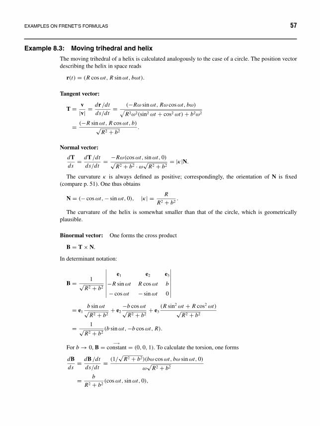
EXAMPLES ON FRENET’S FORMULAS 57
Example 8.3: Moving trihedral and helix
The moving trihedral of a helix is calculated analogously to the case of a circle. The position vectordescribing the helix in space reads
r(t) = (R cos ωt, R sin ωt, bωt).
Tangent vector:
T = v|v| = dr /dt
ds/dt= (−Rω sin ωt, Rω cos ωt, bω)√
R2ω2(sin2 ωt + cos2 ωt) + b2ω2
= (−R sin ωt, R cos ωt, b)√R2 + b2
.
Normal vector:
dTds
= dT /dt
ds/dt= −Rω(cos ωt, sin ωt, 0)√
R2 + b2 · ω√
R2 + b2= |κ|N.
The curvature κ is always defined as positive; correspondingly, the orientation of N is fixed(compare p. 51). One thus obtains
N = (− cos ωt, − sin ωt, 0), |κ| = R
R2 + b2.
The curvature of the helix is somewhat smaller than that of the circle, which is geometricallyplausible.
Binormal vector: One forms the cross product
B = T × N.
In determinant notation:
B = 1√R2 + b2
∣∣∣∣∣∣∣∣e1 e2 e3
−R sin ωt R cos ωt b
− cos ωt − sin ωt 0
∣∣∣∣∣∣∣∣= e1
b sin ωt√R2 + b2
+ e2−b cos ωt√
R2 + b2+ e3
(R sin2 ωt + R cos2 ωt)√R2 + b2
= 1√R2 + b2
(b sin ωt, −b cos ωt, R).
For b → 0, B = −→constant = (0, 0, 1). To calculate the torsion, one forms
dBds
= dB /dt
ds/dt= (1/
√R2 + b2)(bω cos ωt, bω sin ωt, 0)
ω√
R2 + b2
= b
R2 + b2(cos ωt, sin ωt, 0),

58 THE MOVING TRIHEDRAL (ACCOMPANYING DREIBEIN)—THE FRENET FORMULAS 8
dBds
= −τN .
The vector N has already been calculated above: N = (− cos ωt, − sin ωt, 0). From there followsthe torsion of the helix. It holds that
−τ = −b
R2 + b2, τ = b
R2 + b2.
The torsion radius: σ = 1/τ = (R2 + b2)/b.For b = 0, it follows that τ = 0. τ is a measure for the variation of B, i.e., for dB /ds. In other
words: τ is a measure of how the curve is winding out of the plane.
The three unit vectors T, N, and B define three planes that have particular names:
T and N span the osculating plane,
N and B span the normal plane,
B and T span the rectifying plane.
Remark: For a straight line r(t) = a + te κ = 0 ( = ∞) and τ = 0 (σ = ∞). N andB may then be put arbitrarily ⊥ to T = e. This is quite clear.
Velocity and acceleration of a mass point on an arbitrary space curve: For arbitraryspace curves it is sometimes convenient to express the velocity and the acceleration bymeans of the new unit vectors. After introducing the vector T one has
T = v|v| , v = |v| · T = vT.
This relation may be used to derive the acceleration.
b = d2rdt2
= dvdt
= d
dt(v T) = dv
dtT + v
dTdt
.
By transforming the second term, one obtains for the acceleration
dTdt
= dTds
ds
dt= dT
dsv,
b = dv
dtT + v2 dT
ds= dv
dtT + v2κN = dv
dtT + v2
N.
The acceleration is composed of two components: the tangential acceleration dv/dt Tpointing in the tangential direction, and the centripetal acceleration v2/ N pointing towardthe center of the circle of curvature. For a uniform motion of a mass point on a circle(Example 7.4) there exists only the centripetal acceleration, because dv/dt = 0 due to theuniformity of motion.

EXAMPLES ON FRENET’S FORMULAS 59
J( )tJ( )t
T
TJ
r( )t
r( )t sP0
P1
Parallel evolvents J(t) belonging to thecurve r(t).
The Evolute and the Evolvent: The evoluteE (t) of a curve r(t) is the geometric position ofthe centers of curvature (centers of the osculatingcircles) of the curve r(t):
E (t) = r(t) + (t)N(t)
= r(t) + 1
κ(t)N(t) ,
where 1/κ = is the curvature radius of the curveat point r. For plane curves, (τ = 0) this holds:The tangents of the evolutes are simultaneouslynormals of the initial curve, because
dEdt
= drdt
+ d
dtN(t) +
dNdt
= Tds
dt+ d
dtN(t) +
ds
dt(τB − κT)
= T(
ds
dt− κ︸︷︷︸
=1
ds
dt
)+ d
dtN (because τ = 0)
= d
dtN.
The evolvent (or involute or unwinding curve) J(t) is the geometric position of the arclength s plotted along the tangents:
J(t) = r(t) − s(t) · T(t).
s is measured from an initial point P0. Depending on the choice of the initial point P0,one obtains a family of curves, whereby two evolvents in each point have a constantrelative distance in normal direction. Such curves are called parallel curves. This is seenimmediately by demonstrating that the tangent to the evolvent is perpendicular to thetangent of the initial curve, i.e., T · TJ = 0. But this is evident because
TJ ∼ dJdt
= ds
dtT − ds
dtT︸ ︷︷ ︸
=0
−s(t)dTdt
; thus TJ ∼ −N.
If one is dealing with plane curves, then the construction of the evolutes and of theevolvents are in some kind of inverse relation with respect to each other. One finds:
I. One of the evolvents of an evolute is the initial curve itself, symbolically written as
JEr(s) = r(s).
II. The evolute of each evolvent of a curve is the initial curve itself, that is,
EJr(s) = r(s).

60 THE MOVING TRIHEDRAL (ACCOMPANYING DREIBEIN)—THE FRENET FORMULAS 8
Here we have written the corresponding initial curve as an index; thus Jr(s) is theevolvent of the curve r(s), and EJr(s) is again the evolute of the evolvent Jr(s).
We prove the second assertion: It reads
EJr(s) = Jr (s) + 1
κJNJ = (r(s) − sTr (s)) + 1
κJNJ .
The normal of the curve Jr is obtained by differentiation of the tangent vector TJ = −Nr
with respect to the arc length sJ (i.e. not with respect to s ≡ sr !). Therefore,
NJ = 1
κJ
dTJ
dsJ= 1
κJ
ds
dsJ
(−dNr
ds
)= − 1
κJ
ds
dsJ(τBr − κTr) = κ
κJ
ds
dsJTr
if the torsion τ vanishes (plane curve!).The derivative of the arc length of the curve r with respect to the arc length of the evolvent
Jr is obtained because
TJ = dJr
dsJ= dJr
ds
ds
dsJ; thus
ds
dsJ=
∣∣TJ∣∣
|dJr /ds| = 1
s|dTr/ds| = 1
sκ.
Because NJ and Tr are unit vectors, it must hold that
κ
κJ
ds
dsJ= 1 or κJ = κ
ds
dsJ= κ
1
sκ= 1
s.
We see that the curvature radius of the evolvent just equals the corresponding arc lengths of the “unwound” curve, as is expected clearly.
For the evolute of the evolvent, we now obtain
EJr = r(s) − sTr(s) + 1
κJNJ
= r(s) − sTr(s) + 1
κJTr(s)
= r(s) − sTr(s) + sTr(s) = r(s).
Thus, assertion II is proved. Assertion I may be proved in a similar way.
Note: By adding a term pointing along the binormal direction, the definition of the evolutemay be generalized in such a way that the assertion holds also for general space curveswith torsion τ = 0 (compare to Example 8.6).

EXAMPLES ON FRENET’S FORMULAS 61
Example 8.4: Evolvent of a circle
The evolvent of a circle is a spiral. The centers of curvature of this spiral are located on the circle,which therefore is the evolute of the spiral (compare the figure).
P0
P1
MEvolute
Evolvent
Evolvent
The circle and two of its evolvents.
Problem 8.5: Arc length
zy
x
The space curve.
Calculate the arc length of the space curve given by
r(t) = 3 cosh(2t) ex + 3 sinh(2t) ey + 6tez
for the interval 0 ≤ t ≤ π . Outline the curve!
Solution One has
s =∫
ds =∫
ds
dtdt =
∫ ∣∣∣∣drdt
∣∣∣∣ dt,
because ds = |dr|,drdt
= 6 sinh(2t) ex + 6 cosh(2t) ey + 6ez,∣∣∣∣drdt
∣∣∣∣ = 6√
sinh2(2t) + cosh2(2t) + 1 = 6√
2 cosh2(2t),
because sinh2 x = cosh2 x − 1 → |dr /dt | = 6√
2 cosh(2t),
s =π∫
0
6√
2 cosh(2t) dt = 1
26√
2
2π∫0
cosh x dx = 3√
2 sinh(2π).
The space curve comes from the first octant, intersects the x, y-plane at the point (3,0,0), and entersthe eighth octant—twisted hyperbola: Consider the x, y-components: x = cosh 2t, y = sinh 2t, thenform x2 − y2 = cosh2 2t − sinh2 2t = 1 → x2 − y2 = k (k = constant). This is the equation of ahyperbola, see Chapter 26.

62 THE MOVING TRIHEDRAL (ACCOMPANYING DREIBEIN)—THE FRENET FORMULAS 8
Example 8.6: Generalization of the Evolute
The definition of the evolute may be extended to the case of nonplanar curves, i.e., curves with torsionτ(s) = 0 in such a way that
JEr(s) = r(s) (8.13)
further holds. For this purpose we start from a general ansatz allowing that the evolute runs out ofthe osculating plane of the curve r(s), namely
E(s) = r(s) + λ(s)N(s) + µ(s)B(s) (8.14)
with two indeterminate functions λ(s) and µ(s).To calculate the evolvent of E, one needs the derivative
dEds
= drds
+ dλ
dsN + λ
dNds
+ dµ
dsB + µ
dBds
= T(1 − κλ) + N(λ − µτ) + B(µ + τλ), (8.15)
where the Frenet formulas have been utilized. The dot denotes differentiation with respect to s.The evolvent of the evolute then has the form
JEr(s) = Er(s) − sE (s)TE(s) = Er(s) − sE (s)dEdsE
(s)
= r + λN + µB − sEds
dsE
dEds
= r − ds
dsEsE T(1 − κλ) + N
[λ − sE
ds
dsE
(λ − µτ
)]+ B
[µ − sE
ds
dsE(µ + τλ)
]. (8.16)
In order to fulfill 8.13, all additional terms on the right side of 8.16 must vanish. Because thevectors of the moving trihedral are orthogonal, one is led to three independent equations:
1 − κλ = 0; (8.17)
λ − sEds
dsE(λ − µτ) = 0; (8.18)
µ − sEds
dsE(µ + τλ) = 0. (8.19)
The first equation again yields the old result
λ(s) = 1
κ(s). (8.20)
We now resolve equation 8.18:
sEds
dsE= λ
λ − µτ= 1/κ
(−1/κ2)κ − µτ= −κ
κ + µτκ2(8.21)

EXAMPLES ON FRENET’S FORMULAS 63
and insert this in equation 8.19:
µ + κ
κ + µτκ2(µ + τλ) = 0. (8.22)
This is a differential equation of first order for the function µ(s),
µ + τκµ2 + κ
κµ + τ
κ= 0. (8.23)
In order to solve 8.23, we multiply by κ ,
(κµ + κµ) + τκ2µ2 + τ = 0. (8.24)
We substitute Y (s) = κ(s)µ(s); hence
d
dsY + τ
(Y 2 + 1
) = 0. (8.25)
This may be integrated by separation of variables,
−∫
dY
Y 2 + 1= +
∫ds τ + C,
hence
+arccotY =s∫
0
ds ′τ(s ′) + C
or
µ(s) = 1
κ(s)cot
⎛⎝ s∫0
ds ′ τ(s ′) + C
⎞⎠ . (8.26)
The generalized definition of the evolute therefore reads
E(s) = r(s) + 1
κ(s)N(s) + 1
κ(s)cot
⎛⎝ s∫0
ds ′ τ(s ′) + C
⎞⎠B(s) . (8.27)
Because C is an arbitrary constant, there exists an entire set of evolutes.

9 Surfaces in Space
u v
uv
z
x
y
v1v2
v3
r( , )3
r(,
)1
r(,
)2u
v
Illustration of the space curves r(u, vn).
It may happen that the position vector is not a func-tion of one parameter only but depends on two pa-rameters u and v:
r(u, v) = (x(u, v), y(u, v), z(u, v)).
The position vector then describes a surface inspace. This shall be visualized: Let r be a func-tion of two parameters u and v. We first choose afixed value v1 for v and let u vary continuously.r(u, v1) then describes a space curve (compare tothe figure).
Now we choose another fixed value of v that isnot widely spaced from v1 and denote it by v2. u isagain varied continuously.
There results a space curve r(u, v2) that does not differ too much from r(u, v1). Thisprocedure may be repeated many times, and one obtains many neighboring space curves(see figure overleaf).
Then, the same procedure may be performed in the opposite manner. By choosing a fixedvalue for u and varying v continuously, one obtains distinct neighboring lines r(un, v) fora fixed un (see next figure).
If the spacings between u and v become more and more dense, one obtains a surfacein space. One may form the derivative along such a curve (e.g., fixed u = u2 and varyingv). The derivative in which one of the parameters is considered variable while the otherparameters are considered fixed is called a partial derivative and is denoted by a round ∂
(spoken: “d partial” or “d partially derived with respect to”).
u = ui = constant :dr(ui , v)
dv= rv = ∂r(u, v)
∂v.
64

SURFACES IN SPACE 65
z
x
y
v1 v2 v3
v4v5
v6
v7v8
v9
Coordinate lines with varying u are characterized by fixed values of v1, v2, . . . .
z
x
y
v v
u
u
u
u
vv
vv
vv
v
uv1 2
2
1
3
4
34
5
67
89
r(,
)
The net of coordinate lines.
In the same way one forms the tangent vector ru :
v = vi = constant :dr(u, vi )
du= ru = ∂r(u, v)
∂u.
The plane fixed by ru and rv is called the tangent plane of the surface. From ru and rv , oneeasily forms the normal vector n, which is perpendicular to the tangent plane.

66 SURFACES IN SPACE 9
z
x
y
rv
ru
n
Illustration of a surface in space withtangent and normal vectors and a tan-gent plane in one point of the surface.
The normal vector is
n(u, v) = ru × rv
|ru × rv| .
If ru · rv = 0 at any point of the surface, the meshformed by the curves for u = constant and v =constant, respectively, is called an orthogonal mesh.For example, the meridians and parallels of constantlatitude of a sphere form an orthogonal mesh. A sur-face for which a normal vector may be constructedat any point is called orientable. There are surfaceswith only one side, as for example the Mobius strip(see Section 14). On such a surface, any point can bereached from any other point by a continuous dis-placement of the normal vector. Such surfaces arenot orientable. Orientable surfaces have inner and outer sides. By a continuous displacementof the normal vector, one stays always on the same side of a orientable surface. The normaln of an orientable surface is defined as positive for external (convex) surfaces, and negativefor concave ones.
Example 9.1: Normal vector of a surface in space
The position vector r(u, v) = a cos u sin v e1 + a sin u sin v e2 + a cos v e3 with variable parametersdescribes a surface in space.
Find the normal vector as a function of u and v.
Solution ru = −a sin u sin v e1 + a cos u sin v e2 + 0 e3,
rv = a cos u cos v e1 + a sin u cos v e2 − a sin v e3,
ru × rv =
∣∣∣∣∣∣∣∣e1 e2 e3
−a sin u sin v a cos u sin v 0
a cos u cos v a sin u cos v −a sin v
∣∣∣∣∣∣∣∣= −a2 cos u sin2 v e1 − a2 sin u sin2 v e2 − a2 sin v cos v e3 ,
|ru × rv| = a2√
cos2 u sin4 v + sin2 u sin4 v + sin2 v cos2 v
= a2√
(cos2 u + sin2 u) sin4 v + sin2 v cos2 v
= a2√
sin2 v (sin2 v + cos2 v)
= a2| sin v|,n = (− cos u sin v, − sin u sin v, − cos v) for sin v > 0.

SURFACES IN SPACE 67
The result means that the normal vector always points opposite to the position vector, which is thecase for a sphere. One may easily prove that the function of the position vector represents a sphere,by calculating the magnitude of the position vector:
x = a cos u sin v,
y = a sin u sin v,
z = a cos v .
The absolute value (the normalization) |r| = r of the position vector is calculated from
|r|2 = x2 + y2 + z2 = a2(cos2 u sin2 v + sin2 u sin2 v + cos2 v)
= a2(sin2 v (cos2 u + sin2 u) + cos2 v)
= a2.
From there it follows that r = a = constant, i.e., the given position vector determines the surfaceof a sphere.
Because
ru · rv = −a2 sin u cos u sin v cos v + a2 sin u cos u sin v cos v + 0 (−a sin v) = 0,
the mesh spanned by the u, v-lines represents orthogonal coordinates. One easily confirms that theu-v-lines are the meridians and parallels of equal latitude on a sphere.

10 CoordinateFrames
In an n-dimensional space one may always define n linearly independent base vectors outof which any arbitrary vector may be composed by a linear combination. For the sake ofsimplicity, vectors of magnitude unity are usually adopted as base vectors.
Corresponding to the number of base vectors, the position of an arbitrary point maybe specified by n independent real numbers ui , i = 1, . . . , n. Each coordinate frameis characterized by a mutually unique assignment between the space points and these nnumbers, the coordinates.
A vector in the n-dimensional space reads
r =n∑
i=1
ui ei ,
where the n base vectors ei again shall satisfy the orthonormality relation ei · ej = δi, j .The scalar product of two n-dimensional vectors a = ai and b = bi may be defined bya · b = ∑n
i=1 ai bi , in analogy to the three-dimensional space.The introduction of a coordinate frame implies that the coordinates of a space-fixed point
change if the frame is displaced or rotated. From there it follows that for any special systema reference point and a definite orientation in space must be given.
Physically seen, both quantities may be fixed by tying the coordinate frame, for example,in a rigid body as a reference body; in a completely empty space it would make no sense tospeak of the position of a point. Of course, a coordinate frame must not be “at rest” (e.g.,all frames tied to the earth are accelerated frames due to the earth’s rotation).
Special examples
s
A caterpillar on a bladeof grass.
1. The position of a point on an arbitrarily curved line (n = 1)
is already specified by giving one number. In the simplest caseone adopts the arc length s measured from a reference point ina defined direction of motion as a “natural parameter.” This is aone-dimensional space.
68

COORDINATE FRAMES 69
An ant crawling on a sphere.
2. The surface of the earth, although being formed ina highly complicated manner (mountains, etc.), is anarea with n = 2. Each point on it may thus be uniquelydetermined by two numbers. As is known this may beachieved by fixing two angular quantities: geogra-phic length and latitude. Arbitrarily chosen referencequantities are the zero meridian through Greenwich(geographic length = 0) and the equator (geographiclatitude = 0). This is a two-dimensional space.
In order to change from one coordinate frame (q1, q2, q3) to another one (here specificallythe Cartesian frame: x, y, z), the following equations have to be set up:
Transformation equations:
q1 = q1(x, y, z) x = x(q1, q2, q3)
q2 = q2(x, y, z) and their inversion y = y(q1, q2, q3)
q3 = q3(x, y, z) z = z(q1, q2, q3).
(10.1)
Z
X
Y
y
x
z P
0
e3
e2e1
r
The definition of Cartesian coordinates.
Cartesian coordinates: Given are the three basevectors e1, e2, e3 along the directions of three mu-tually perpendicular axes. The coordinates x, y, zof a point P are the projections of the position
vector r = −→O P onto the axes,
r = xe1 + ye2 + ze3, |ei | = 1.
By convention the three unit vectors form aright-handed frame. Because they are mutuallyperpendicular, they constitute an orthogonal frame.Moreover, the unit vectors are always parallel tothe axes, that is, fully independent of the positionof the point P in space.
This constancy of direction of the unit vectors combined with their orthogonality isthe reason for preferred usage of Cartesian coordinates. For many special problems withparticular symmetry, it turns out as convenient to use coordinate frames that are adapted tothe geometric conditions and therefore simplify the calculations. For example, the motionof a plane pendulum may be described in terms of one angular coordinate, the motion of aspherical pendulum in terms of two angular quantities.
Curvilinear coordinate frames: To explain the denotation, we suppose the coordinatesx, y, z of r to be expressed by q1, q2, q3 according to (10.1). There results
r(q1, q2, q3) = x(q1, q2, q3), y(q1, q2, q3), z(q1, q2, q3) .

70 COORDINATE FRAMES 10
Two of these three coordinates q1, q2, q3 are now kept constant; let only the third one bevariable. All points satisfying this condition are located on a space curve. There arise thethree coordinate lines:
L1 : r = r(q1 , q2 = c2, q3 = c3),
L2 : r = r(q1 = c1, q2 , q3 = c3), (10.2)
L3 : r = r(q1 = c1, q2 = c2, q3 ).
As is immediately seen from the scheme, the three coordinate lines have exactly onecommon intersection point P (c1, c2, c3).
In the Cartesian frame these lines are straight lines parallel to the three axes. If, however,at least one of the lines is not straight, one speaks of curvilinear coordinates. One may stillproceed one step further and keep only one of the three coordinates constant, while theother two remain variable. There arise two-dimensional (in general curved) areas in space.
Coordinate areas:
F1 : r = r(q1 = c1, q2 , q3),
F2 : r = r(q1 , q2 = c2, q3), (10.3)
F3 : r = r(q1 , q2 , q3 = c3).
z
y
x
q3 curve
q2 curveq1 curve
P
q c1 1=
q c3 3=
q c2 2=
Illustration of coordinate surfaces.
One may imagine the coordinate linesas resulting from the intersection of two ofthese areas. In the Cartesian system the co-ordinate areas are planes with the commonpoint P .
Generally an arbitrary point may be rep-resented as the intersection point of its threecoordinate areas (and, of course, also co-ordinate lines). One presupposes that eachspace point is traversed by exactly one areafrom each of the three sets of coordinateareas. The three fixed parameters of theseareas are the coordinates of the point.
The vector r(q1, q2, q3) as a function of the three parameters q1, q2, q3 describes a spaceregion. Actually, if one of the coordinates is kept fixed, e.g., q3 = q3, according to Chapter 9we are dealing with an area in space. If q3 changes to q3 = q3 + q3, a neighboring areaemerges. If q3 is running continuously, there emerge more and more arbitrarily denselylocated areas in space that, in total, cover a space region.
General specification of base vectors: As normalized base vector (unit vector) eq1 atpoint P , we choose a vector of magnitude 1 tangential to the coordinate line q2 = c2, q3 = c3
at P . Its orientation shall correspond to the direction of passage of the coordinate line withincreasing value q1.

COORDINATE FRAMES 71
This introduction of the unit vector corresponds exactly to the geometric meaning ofthe partial derivative; hence, eq1 may be calculated by partial differentiation of the positionvector with respect to q1 and subsequent normalization:
eq1 = ∂r /∂q1
|∂r /∂q1| or∂r∂q1
= h1eq1 or∂r∂qi
= hi eqi ; i = 1, 2, 3. (10.4)
Here hi are scaling factors, namely hi = |∂r/∂qi |. In curvilinear coordinate frames thedirection of at least one of the coordinate lines changes by definition. Therefore, theseframes are, contrary to the Cartesian frame, coordinate frames with variable unit vectors.
ez
eϕ
eρr
Z
X
Y
zP
ρϕ
ρ ϕsin
ρ ϕcos
The definition of cylindrical coordinates.
Cylinder coordinates: The coor-dinates used are
ϕ: angle between the projection ofthe position vector onto the x, y-plane and the x-axis,
: separation of the point from thez-axis,
z: length of the projection of the po-sition vector onto the z-axis (as inthe Cartesian frame).
The coordinate areas extend to in-finity (see figure, showing limitedsections) and are
= 1: circular cylinders about the z-axis,
ϕ = ϕ1: half-planes containing the z-axis, (10.5)
z = z1: planes parallel to the x, y-plane.
Coordinate lines are two straight lines and a circle.
Transformation equations: From the figure one may directly read off the relations:
r = (x1, x2, x3) = ( cos ϕ, sin ϕ, z)
or in detail:
x = cos ϕ, = √x2 + y2,
y = sin ϕ, ϕ = arctany
x= arcsin
y
,
z = z, z = z.
(10.6)

72 COORDINATE FRAMES 10
To ensure that one point cannot be characterized by distinct combinations of coordinates,we agree on the following restrictions:
≥ 0; 0 ≤ ϕ < 2π.
The representation is not completely unique since the angle remains indefinite for pointswith = 0. But inversely—and this is the more important requirement—to each triple, ϕ, z only one space point is associated.
ρ ϕ
y
z
ez
eϕ
eρ
X
Z
Yx
P
ϕ
( , , )z
ρ
Illustration of cylindrical coordinates.
Unit vectors: According to the geometricintroduction as tangent vectors to the coordi-nate lines, the unit vectors e, eϕ , ez are givenby
e = ∂r /∂
|∂r /∂| = (cos ϕ, sin ϕ, 0)
1,
eϕ = ∂r /∂ϕ
|∂r /∂ϕ| = (− sin ϕ, cos ϕ, 0)
,
ez = ∂r /∂z
|∂r /∂z| = (0, 0, 1)
1. (10.7)
e is parallel to the x, y-plane and points inradial direction from the z-axis outward.
eϕ is tangent to the circle z = z1, = 1,that is, also parallel to the x, y-plane.
ez corresponds to the Cartesian e3.
Thus, e and eϕ may be projected onto the x, y-plane without any changes. One has
e = cos ϕ e1 + sin ϕ e2,
eϕ = cos(ϕ + π
2
)e1 + sin
(ϕ + π
2
)e2 = − sin ϕ e1 + cos ϕ e2,
e = (cos ϕ, sin ϕ, 0),
eϕ = (− sin ϕ, cos ϕ, 0), (10.8)
ez = (0, 0, 1).
The same result follows by partial differentiation of r with respect to , ϕ, z and subsequentnormalization (see equation (10.7)).
To check the unit vectors, we form the triple scalar product
e · (eϕ × ez) =
∣∣∣∣∣∣∣∣cos ϕ sin ϕ 0
− sin ϕ cos ϕ 0
0 0 1
∣∣∣∣∣∣∣∣ = 1.

COORDINATE FRAMES 73
This is the unit volume spanned by the vectors e, eϕ, ez . Thus, the cylindrical coordinatesform an orthogonal frame with variable unit vectors. For solving kinematic problems it isimportant to know the derivative of the unit vectors with respect to time. Let the functions(t), ϕ(t), z(t) be known. The generalization of the chain rule for a function of severalvariables then yields
de
dt= ∂e
∂
d
dt+ ∂e
∂ϕ
dϕ
dt+ ∂e
∂z
dz
dt
= 0 + (− sin ϕ, cos ϕ, 0)ϕ + 0 = ϕ eϕ,
deϕ
dt= (− cos ϕ, − sin ϕ, 0)ϕ = −ϕ e, (10.9)
dez
dt= 0.
The derivative of a vector e of constant magnitude has no component along the directionof e and hence must be perpendicular to it: e · e = constant ⇒ e · de/dt = 0!
The equations given above fulfill this condition! We still note that from now on we shallfrequently abbreviate the time derivative of a quantity by a dot above this quantity, as, forexample, dϕ/dt ≡ ϕ or de/dt ≡ e, etc.
Velocity and acceleration in cylindrical coordinates: Let a point move along a pathdescribed by the position vector r(t). One has
(a) the velocity v(t) = dr/dt ,
(b) the acceleration b(t) = d2r/dt2 = dv/dt .
In cylindrical coordinates let (t), ϕ(t), z(t) be given. The position vector is
r = e + zez . (10.10)
Note: These base vectors are now not fixed but are coordinate-dependent by themselves.One has to take care in component representation: For instance one cannot simply dif-ferentiate r = (, 0, z)! In order to avoid errors, one has to write out the vector, as, forexample,
(a)
r = e + e + zez + zez .
This yields the velocity:
r = e + ϕeϕ + zez . (10.11)
(b)
r = (e + e) + (ϕeϕ + ϕeϕ + ϕeϕ) + (zez + zez).

74 COORDINATE FRAMES 10
This yields the acceleration:
r = ( − ϕ2)e + (ϕ + 2ϕ)eϕ + zez . (10.12)
Hence, in the cylindric frame both the velocity and acceleration are composed of threecomponents: a radial component, an azimuthal component, and a component in the z-direction.
Spherical coordinates According to the figure below, the coordinates are
r : length of the position vector,
ϑ : angle between the position vector and the z-axis (polar angle),
ϕ: azimuth (as in the cylindric frame).
Z
X
Yy
z
er
eϕ
eϑx ϕ
ϑP r( ,ϑ ϕ, )r
The definition of spherical coordinates.
The previous figure illustrates the various coor-dinate areas and lines. The point P is the inter-section point of a circular cone about the z-axiswith the vortex at the origin 0, a half-plane includ-ing the z-axis, and a sphere with the center at 0that results by keeping the radius r constant andvarying the two angles. The coordinate lines aretwo circles and a straight line: (1) r = constant,ϕ = constant, ϑ variable — meridian; (2) r =constant, ϑ = constant, ϕ variable — parallel ofconstant latitude; (3) ϕ = constant, ϑ = constant,r variable — radial ray.
The coordinate areas are a conical area (ϑ =constant), a half-plane (ϕ = constant), and aspherical area (r = constant).
Transformation equations
r = x1e1 + x2e2 + x3e3 = r sin ϑ cos ϕ e1 + r sin ϑ sin ϕ e2 + r cos ϑ e3.
When the equations are written in detail, we get
x = r sin ϑ cos ϕ, r = √x2 + y2 + z2,
y = r sin ϑ sin ϕ, ϕ = arctany
x,
z = r cos ϑ, ϑ = arctan(√
x2 + y2/z)
.
(10.13)

COORDINATE FRAMES 75
ez
eϑ
eϕ
eρer
eϕ
X
X
XX
X
X
Z
Z
Z Z
Z
Z
Y
Y
Y Y
Y
Y
P
ϕ
ϕ ϕ
ϑ
ϕ
ϑ
ρ
ρ = const.
ϑ = const.
ϕ = const. ϕ = const.
z = const.
r = const.
r
z
ϕ ϕ
ϑ
Coordinate surfaces and coordinate lines for cylindrical coordinates (left) and spherical coordinates (right).

76 COORDINATE FRAMES 10
To reach uniqueness, the following restrictions are agreed upon:
r ≥ 0, 0 ≤ ϕ < 2π, 0 ≤ ϑ < π. (10.14)
Unit vectors for spherical coordinates: The position vector is
r = r(sin ϑ cos ϕ, sin ϑ sin ϕ, cos ϑ).
Partial differentiation yields
∂r∂r
= (sin ϑ cos ϕ, sin ϑ sin ϕ, cos ϑ), hr =∣∣∣∣∂r∂r
∣∣∣∣ = 1,
∂r∂ϑ
= r(cos ϑ cos ϕ, cos ϑ sin ϕ, − sin ϑ), hϑ =∣∣∣∣ ∂r∂ϑ
∣∣∣∣ = r,
∂r∂ϕ
= r(− sin ϑ sin ϕ, sin ϑ cos ϕ, 0), hϕ =∣∣∣∣ ∂r∂ϕ
∣∣∣∣ = r sin ϑ.
(10.15)
The unit vectors follow by normalization:
er = (sin ϑ cos ϕ, sin ϑ sin ϕ, cos ϑ);eϑ = (cos ϑ cos ϕ, cos ϑ sin ϕ, − sin ϑ); (10.16)
eϕ = (− sin ϕ, cos ϕ, 0).
Geometrical interpretation: One has rer = r; hence, er points along the position vector,that is, it is the normal to the surface of the sphere.
eϕ lies tangential to the circle r = r1, ϑ = ϑ1, namely, parallel to the x, y-plane. Itscomponent representation may accordingly be seen from the previous figure when settingthe circle radius equal to r sin ϑ .
eϑ has a component sin ϑ along the negative z-direction. We know that eϑ is the tangentvector of the ϑ-coordinate line, namely the tangent to the meridian. The question whether eϑ
points upward or downward is decided by the z-component (− sin ϑ): eϑ points downwardas in the figure.
One may easily convince oneself that the spherical coordinates also constitute anorthogonal frame with variable unit vectors, by evaluating the triple scalar producter · (eϑ × eϕ) = 1.
We write the equations (10.16) explicitly:
er = sin ϑ cos ϕ e1 + sin ϑ sin ϕ e2 + cos ϑ e3;eϑ = cos ϑ cos ϕ e1 + cos ϑ sin ϕ e2 − sin ϑ e3; (10.17)
eϕ = − sin ϕ e1 + cos ϕ e2 + 0 e3.

COORDINATE FRAMES 77
and solve them for e1, e2, e3 according to Cramer’s rule1. For example, for e1 one finds
e1 =
∣∣∣∣∣∣∣∣er sin ϑ sin ϕ cos ϑ
eϑ cos ϑ sin ϕ − sin ϑ
eϕ cos ϕ 0
∣∣∣∣∣∣∣∣ //∣∣∣∣∣∣∣∣
sin ϑ cos ϕ sin ϑ sin ϕ cos ϑ
cos ϑ cos ϕ cos ϑ sin ϕ − sin ϑ
− sin ϕ cos ϕ 0
∣∣∣∣∣∣∣∣ ,
= er sin ϑ cos ϕ + eϑ cos ϑ cos ϕ + eϕ(− sin ϕ)
sin2 ϑ cos2 ϕ + cos2 ϑ cos2 ϕ + sin2 ϕ,
e1 = sin ϑ cos ϕ er + cos ϑ cos ϕ eϑ − sin ϕ eϕ, (10.18)
and similarly for e2 and e3:
e2 = sin ϑ sin ϕ er + cos ϑ sin ϕ eϑ + cos ϕ eϕ;e3 = cos ϑ er − sin ϑ eϑ . (10.19)
Velocity and acceleration in spherical coordinates: To calculate the velocity and ac-celeration in spherical coordinates, we still need the time derivatives er , eϑ , eϕ . One finds
er = ∂er
∂ϑϑ + ∂er
∂ϕϕ
= (cos ϑ cos ϕ, cos ϑ sin ϕ, − sin ϑ)ϑ + (− sin ϑ sin ϕ, sin ϑ cos ϕ, 0)ϕ
= ϑeϑ + sin ϑϕeϕ, (10.20)
and similarly
eϑ = −ϑ er + cos ϑ ϕ eϕ,
eϕ = − sin ϑ ϕ er − cos ϑ ϕ eϑ . (10.21)
Now we may calculate the velocity in spherical coordinates. The following hold:
r = rer ,
r = rer + r er
= rer + r ϑeϑ + r sin ϑ ϕ eϕ, (10.22)
r = rer + r er + r ϑeϑ + r ϑeϑ + r ϑ eϑ
+ r sin ϑ ϕ eϕ + r cos ϑ ϑ ϕ eϕ + r sin ϑ ϕ eϕ + r sin ϑ ϕ eϕ
(after inserting (10.20) and (10.21) )
1Gabriel Cramer, b. July 31, 1704, Geneva, as son of a physician—d. Jan. 4, 1752, Bagnols near Nımes. Afterhis studies at the university of Geneva, Cramer became appointed as professor for philosophy and mathematics.From 1727-1729 he made an informative trip through many European countries. After his return home Cramerheld important municipal posts in Geneva. His rapidly decaying state of health led him to southern France wherehe soon died. His main work is the Introduction a l’Analyse des Lignes Courbes Algebriques (1750), where amongother things the theory of solving systems of equations by means of determinants is outlined.

78 COORDINATE FRAMES 10
= (r − r ϑ2 − r sin2 ϑ ϕ2)︸ ︷︷ ︸br
er +(
1
r
d
dt(r2ϑ) − r sin ϑ cos ϑ ϕ2
)︸ ︷︷ ︸
bϑ
eϑ
+(
1
r sin ϑ
d
dt
(r2 sin2 ϑ ϕ
))︸ ︷︷ ︸
bϕ
eϕ
≡ br er + bϑeϑ + bϕeϕ. (10.23)
If ϑ ≡ π/2, that is, sin ϑ = 1, ϑ = 0, cos ϑ = 0, (10.22) and (10.23) turn into
r = rer + r ϕeϕ
and
r = (r − r ϕ2)er + (2r ϕ + r ϕ)eϕ,
respectively. These expressions for velocity and acceleration in plane polar coordinates arealready known from the discussion on cylinder coordinates.
Problem 10.1: Velocity and acceleration in cylindrical coordinates
k
–k
ϕ 2k
y
x
The heart curve or cardioid.
A particle moves with constant velocity v along the heart curveor cardioid r = k(1 + cos ϕ) (Greek kardia = heart). Find theacceleration a, its magnitude, and the angular velocity. (Notethat r denotes here the coordinate of the cylindrical coordinateframe.)
Solution The differentiation of the path equation with respect to time yields
r = k(1 + cos ϕ), (10.24)
r = −k sin ϕ ϕ, (10.25)
r = −k(ϕ2 cos ϕ + ϕ sin ϕ). (10.26)
For the discussion below it is useful to conclude from 10.24 that
cos ϕ = r
k− 1 and sin2 ϕ = 1 −
( r
k− 1
)2 = 2r
k− r 2
k2. (10.27)
According to 10.25 we obtain
r 2 = k2 sin2 ϕ ϕ2 = k2
(2
r
k− r 2
k2
)ϕ2 = 2kr ϕ2 − r 2ϕ2 . (10.28)
Because we are dealing with plane polar coordinates, we write for the radius vector
r = rer , (10.29)
r = rer + r ϕeϕ, (10.30)
r = (r − r ϕ2)er + (r ϕ + 2r ϕ)eϕ. (10.31)
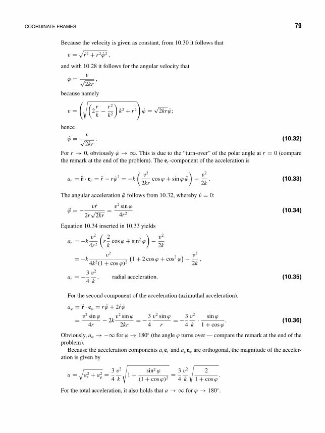
COORDINATE FRAMES 79
Because the velocity is given as constant, from 10.30 it follows that
v =√
r 2 + r 2ϕ2 ,
and with 10.28 it follows for the angular velocity that
ϕ = v√2kr
,
because namely
v =(√(
2r
k− r 2
k2
)k2 + r 2
)ϕ = √
2kr ϕ;
hence
ϕ = v√2kr
. (10.32)
For r → 0, obviously ϕ → ∞. This is due to the “turn-over” of the polar angle at r = 0 (comparethe remark at the end of the problem). The er -component of the acceleration is
ar = r · er = r − r ϕ2 = −k
(v2
2krcos ϕ + sin ϕ ϕ
)− v2
2k. (10.33)
The angular acceleration ϕ follows from 10.32, whereby v = 0:
ϕ = − vr
2r√
2kr= v2 sin ϕ
4r 2. (10.34)
Equation 10.34 inserted in 10.33 yields
ar = −kv2
4r 2
(r
2
kcos ϕ + sin2 ϕ
)− v2
2k
= −kv2
4k2(1 + cos ϕ)2
(1 + 2 cos ϕ + cos2 ϕ
)− v2
2k,
ar = −3
4
v2
k, radial acceleration. (10.35)
For the second component of the acceleration (azimuthal acceleration),
aϕ = r · eϕ = r ϕ + 2r ϕ
= v2 sin ϕ
4r− 2k
v2 sin ϕ
2kr= −3
4
v2 sin ϕ
r= −3
4
v2
k· sin ϕ
1 + cos ϕ. (10.36)
Obviously, aϕ → −∞ for ϕ → 180 (the angle ϕ turns over — compare the remark at the end of theproblem).
Because the acceleration components ar er and aϕeϕ are orthogonal, the magnitude of the acceler-ation is given by
a =√
a2r + a2
ϕ = 3
4
v2
k
√1 + sin2 ϕ
(1 + cos ϕ)2= 3
4
v2
k
√2
1 + cos ϕ.
For the total acceleration, it also holds that a → ∞ for ϕ → 180.
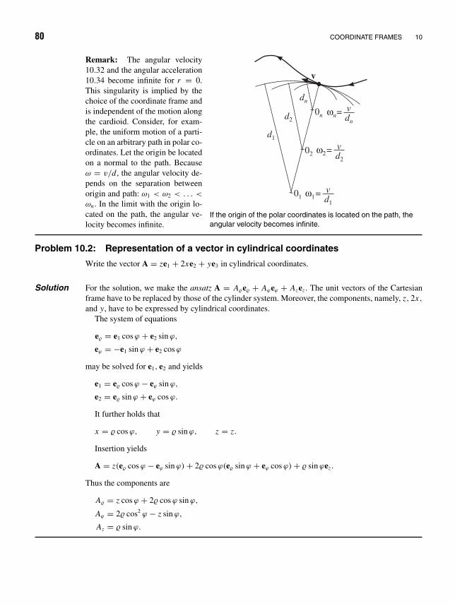
80 COORDINATE FRAMES 10
v
d1
01
d2
02
dn
0n ωn=
ω2=
ω1=
vdn
vd2
vd1
If the origin of the polar coordinates is located on the path, theangular velocity becomes infinite.
Remark: The angular velocity10.32 and the angular acceleration10.34 become infinite for r = 0.This singularity is implied by thechoice of the coordinate frame andis independent of the motion alongthe cardioid. Consider, for exam-ple, the uniform motion of a parti-cle on an arbitrary path in polar co-ordinates. Let the origin be locatedon a normal to the path. Becauseω = v/d, the angular velocity de-pends on the separation betweenorigin and path: ω1 < ω2 < . . . <
ωn . In the limit with the origin lo-cated on the path, the angular ve-locity becomes infinite.
Problem 10.2: Representation of a vector in cylindrical coordinates
Write the vector A = ze1 + 2xe2 + ye3 in cylindrical coordinates.
Solution For the solution, we make the ansatz A = Ae + Aϕeϕ + Azez . The unit vectors of the Cartesianframe have to be replaced by those of the cylinder system. Moreover, the components, namely, z, 2x,
and y, have to be expressed by cylindrical coordinates.The system of equations
e = e1 cos ϕ + e2 sin ϕ,
eϕ = −e1 sin ϕ + e2 cos ϕ
may be solved for e1, e2 and yields
e1 = e cos ϕ − eϕ sin ϕ,
e2 = e sin ϕ + eϕ cos ϕ.
It further holds that
x = cos ϕ, y = sin ϕ, z = z.
Insertion yields
A = z(e cos ϕ − eϕ sin ϕ) + 2 cos ϕ(e sin ϕ + eϕ cos ϕ) + sin ϕez .
Thus the components are
A = z cos ϕ + 2 cos ϕ sin ϕ,
Aϕ = 2 cos2 ϕ − z sin ϕ,
Az = sin ϕ.

COORDINATE FRAMES 81
Problem 10.3: Angular velocity and radial acceleration
a a
S
P1
P2
ωϕ
Motion around P1 with angular ve-locity ω.
A rod rotates about P1 in a plane with the angular velocityω = kesin ϕ . At the time t = 0, let ϕ = 0. The straight lineintersects a fixed circle of radius a at the point P2.
(a) Find the angular acceleration of the rod.
(b) Find the velocity v and the acceleration b of the pointP2 along the rod.
(c) Find the velocity and the acceleration of the point P2 withrespect to the center of the circle.
eϕ
eρ
a 0 a
S
P1
P2
ω
ϕϕ2ϕ
Motion around P1 as seen from O.
Solution (a) The angular velocity is
ω = ϕ = kesin ϕ
⇒ for the angular acceleration
ω = ϕ = kω cos ϕesin ϕ
= k2e2 sin ϕ cos ϕ .
(b) The position vector to the point P2 on the rod is
r = e , where = 2a cos ϕ ⇒ r = 2a cos ϕ e .
The velocity of P2 is obtained from the relation
r = e + ϕeϕ ,
and the acceleration is
r = ( − ϕ2)e + (ϕ + 2ϕ)eϕ .
Insertion yields
v = r = −2a sin ϕ ϕ e + 2a cos ϕ ϕ eϕ
= 2a(− sin ϕ ϕ e + cos ϕϕeϕ
),
b = r = 2a[(−ϕ sin ϕ − 2ϕ2 cos ϕ
)e + (
ϕ cos ϕ − 2ϕ2 sin ϕ)
eϕ
].
For the velocity and acceleration along the rod axis, that is, in the e-direction, one obtains
v = −2aϕ sin ϕ e , b = −2a(ϕ sin ϕ + 2ϕ2 cos ϕ
)e.
The negative sign indicates that both v as well as b point toward the center of rotation P1.(c) The rotation angle of O P2 equals 2ϕ, and the velocity along the circle is
rP2 = a · 2ϕ ⇒ vP2 = 2aϕ = 2akesin ϕ .
The normal acceleration is
bP2b = v2P2
a= 4ak2e2 sin ϕ ,

82 COORDINATE FRAMES 10
the tangential acceleration is
bP2r = dvP2
dt= 2aϕ = 2ak2 cos ϕ e2 sin ϕ ,
and the total acceleration is
bP2 =√
b2P2b + b2
P2r = 2ak2e2 sin ϕ√
4 + cos2 ϕ .

11 Vector DifferentialOperations
Scalar fields: The notion of scalar field means a function φ(x, y, z) that assigns a scalar,the value φ(x1, y1, z1), to any space point P(x1, y1, z1). Examples are temperature fieldsT (x, y, z) and density fields (x, y, z) (e.g., mass density, charge density).
Vector fields: A vector field correspondingly means a function A(x, y, z) that assigns avector A(x1, y1, z1) to any space point P(x1, y1, z1).
Vector fields are, for instance, electric and magnetic fields, characterized by the fieldstrength vectors E and H, or velocity fields υ(x, y, z) in flowing liquids or gases.
The operations gradient, divergence, and curl (rotation)
Gradient: Given a scalar field φ(x, y, z), the gradient of the scalar field at a fixed positionP0(x0, y0, z0), denoted by grad φ(x0, y0, z0), is a vector pointing along the steepest ascentof φ, the magnitude of which equals the change of φ per unit length of the path along themaximum ascent at the point P0(x0, y0, z0).
In this way, any point of a scalar field can be associated with a gradient vector. The setof gradient vectors forms a vector field associated to the scalar field. Mathematically theso-defined vector field is given by the relation
A(x, y, z) = grad φ = e1∂
∂xφ + e2
∂
∂yφ + e3
∂
∂zφ. (11.1)
To simplify the mathematical description, the following notation is used:
grad φ = ∇φ, where ∇ = e1∂
∂x+ e2
∂
∂y+ e3
∂
∂z.
(∇: spoken “nabla” or “nabla operator”.)
83

84 VECTOR DIFFERENTIAL OPERATIONS 11
Definition of an operator: The nabla operator is a symbolic vector (vector operator)that, when applied to a function φ, generates the gradient of φ. Taken as such, the operatoris meaningless; it has to operate on something, for example a scalar function φ(x, y, z).
We now demonstrate that the vector field ∇φ has the properties quoted above. For thispurpose we need the total differential of φ, namely
dφ = ∂φ
∂xdx + ∂φ
∂ydy + ∂φ
∂zdz. (11.2)
This quantity describes the main part of the total increase of the function φ if x changes bydx, y by dy, z by dz, that is,
φ ≈ φ(x + dx, y + dy, z + dz) − φ(x, y, z).
The Taylor expansion up to the first-order term yields
φ(r + dr) = φ(x + dx, y + dy, z + dz)
= φ(x, y, z) + ∂φ
∂xdx + ∂φ
∂ydy + ∂φ
∂zdz + · · · ,
and therefore
φ = φ(r + dr) − φ(r) = ∂φ
∂xdx + ∂φ
∂ydy + ∂φ
∂zdz + · · ·
= dφ + terms of higher order. (11.3)
This explains the name total differential for the main part of the total increase of the functionφ. We thereby have used the Taylor expansion of a function (up to the first terms in thesmall quantities dx, dy, dz). In Section 22 Taylor expansions will be outlined in detail andexplained by numerous examples. We recommend that you have a look at this section now.
Using the infinitesimal position vector dr = (dx, dy, dz), we may also write the totaldifferential as follows:
dφ = ∇φ · dr =(
∂φ
∂x,∂φ
∂y,∂φ
∂z
)· (dx, dy, dz)
= ∂φ
∂xdx + ∂φ
∂ydy + ∂φ
∂zdz . (11.4)
Equipotential surfaces are surfaces on which the function φ takes a constant value,φ(x, y, z) = constant.
As has been shown above, there is the relation
∇φ · dr = dφ, with dr = (dx, dy, dz). (11.5)
Because dφ represents the sum of the increases of φ in each direction dr, dφ = 0 meansto stay on an equipotential surface. For this case, it holds that
0 = dφ = ∇φ · drE S, (11.6)

THE OPERATIONS GRADIENT, DIVERGENCE, AND CURL (ROTATION) 85
ydr
dr
φ
φ
Hill
Minimum
Equipotential lines and the direction of thegradient.
where drE S lies in the equipotential surfaceE S. The scalar product ∇φ · drE S vanishesonly then if the cosine of the enclosed anglevanishes (compare the opposite figure), pro-vided that ∇φ = 0. This implies that ∇φ anddrE S are perpendicular to each other. Thus thegradient of φ is always perpendicular to theequipotential areas.
We now consider the increase dφ along thegradient vector at a fixed point of the scalarfield: Here dr is parallel to ∇φ and then ∇φ ·drtakes the maximum value. Therefore, the vec-tor grad φ = ∇φ always points in the directionof the strongest increase of φ; see the oppositefigure.
Divergence: Contrary to the gradient operation, the divergence is applied to vector fields.Given a vector field A = (Ax , Ay, Az), we further imagine a cuboid-shaped “controlvolume” (rectangular box) with the edge lengths x, y, z.
The “vector flow” across an area represents the entity of vectors penetrating it perpen-dicularly, that is, the normal components of the vectors integrated over the entire area.
y
z xx x x+∆
y y+∆
y
s1s4
s2s3
A y yy y( + )∆ e
A yy y( )e
A x xx x( + )∆ eA xx x( )e
The flow across a cuboid. The extension inthe z-direction (out of the paper plane) isnot shown.
The lateral faces of the cuboid are denoted bys1, s2, . . . , s6.
We now calculate the vector flow across alllateral faces of the cuboid (rectangular box).The edge lengths x, y, z shall be chosenso small that the vector on the cuboid faces maybe considered as nearly constant, such that theintegration of the vector across the faces may bereplaced by a simple summation. We shall countthe vector flow as positive if it flows out of thevolume, and negative if it flows into the volume.
The vector flow through the faces is
s1: −Ax (x)yz,
s2: Ax (x + x)yz,
s3: −Ay(y)xz,
s4: Ay(y + y)xz,
(11.7)
and in the third space direction is
s5: −Az(z)xy,
s6: Az(z + z)xy.(11.8)

86 VECTOR DIFFERENTIAL OPERATIONS 11
A Taylor series expansion up to terms of first order, which is satisfied for small x, y, z,yields
Ax (x + x, y, z) = Ax (x, y, z) + ∂
∂xAx (x, y, z)x + · · · ,
Ay(x, y + y, z) = Ay(x, y, z) + ∂
∂yAy(x, y, z)y + · · · , (11.9)
Az(x, y, z + z) = Az(x, y, z) + ∂
∂zAz(x, y, z)z + · · · .
The terms indicated by dots · · · are of higher order in the small increments x , y, zand may be neglected. The resulting vector flow through the control volume follows bysummation over the lateral faces:(
Ax (x + x, y, z) − Ax (x, y, z))yz
+ (Ay(x, y + y, z) − Ay(x, y, z)
)xz
+ (Az(x, y, z + z) − Az(x, y, z)
)yx,
= ∂
∂xAx (x, y, z)xyz + ∂
∂yAy(x, y, z)xyz + ∂
∂zAz(x, y, z)xyz
=(
∂
∂xAx (x, y, z) + ∂
∂yAy(x, y, z) + ∂
∂zAz(x, y, z)
)V .
Thus the “flow” (total flow) through an infinitesimally small volume (x → dx , y → dy,z → dz) reads
dV ·(
∂
∂xAx + ∂
∂yAy + ∂
∂zAz
). (11.10)
n
nA
A
∆V
Illustration of the divergenceas flow of the vector fieldthrough a volume.
The expression in brackets is called divergence of the vectorfield A:
div A = ∂
∂xAx + ∂
∂yAy + ∂
∂zAz . (11.11)
Thus, the divergence represents the vector flow through avolume V per unit volume. It may also be written in theform
div A = ∇ · A(x, y, z). (11.12)
This last relation may be interpreted as analytic definition. Ashas been shown, it is identical with the geometric definition,namely:
div A = limV →0
flow of the vector field A through V
V= lim
V →0
∫F A · n d F
V. (11.13)
While the argument of the gradient operation is a scalar, the divergence represents thescalar product of the operator ∇ and the vector A. For a vanishing divergence, the total flow

THE OPERATIONS GRADIENT, DIVERGENCE, AND CURL (ROTATION) 87
through an infinitesimal volume equals zero, that is, the in-flow just balances the out-flow.If at some point of the vector field div A > 0, one says that the vector field there has asource; for div A < 0, one speaks of a sink of the vector field. This is immediately clearfrom the definition of the divergence as net flow = out-flow − in-flow per unit volume.
Curl (Rotation):1 The operation curl A assigns a vector field curl A to a given vectorfield A. The vector field curl A informs about possible “vortices” of the field A (a vortexexists if there is a closed curve in the vector field fulfilling the condition that the contourintegral
∮A · ds = 0—see theorem of Stokes). The mathematical formulation of curl A is
given by
1. curl A = ∇ × A, or
2. n · curl A = limF→0(∮
A · ds)/F .
n is a unit normal vector on F . n
∆F
Oriented surfaceelement.
The second definition states that the rotation may also be determinedby forming the contour integral. The integration is performed over thevector field along a curve. More strictly speaking: One integrates overthe projection of A onto ds along the tangent to the curve forming theborder of F . After division by F , this yields the component of curl Aalong n.
The rotation is thus determined by two distinct definitions. The first of these reads indetail
curl A = ∇ × A =
∣∣∣∣∣∣∣∣e1 e2 e3
∂/∂x ∂/∂y ∂/∂z
Ax Ay Az
∣∣∣∣∣∣∣∣= e1
(∂ Az
∂y− ∂ Ay
∂z
)+ e2
(∂ Ax
∂z− ∂ Az
∂x
)+ e3
(∂ Ay
∂x− ∂ Ax
∂y
)(11.14)
nA
A
A
A
∆F
A
Illustration of a vector field A with vorticity onsurface element F with normal vector n.
One has to prove that both definitions are iden-tical. Here we show the identity only for thex-component.
x-component of the curl of A: One mayintegrate about an area F = 4yz in they, z-plane (see the lower figure). n then pointsalong the x-axis, that is, n · curl A just yieldsthe x-component of curl A, namely (curl A)x .
1In German literature, curl is named rotation (rot), so curl A = rot A.

88 VECTOR DIFFERENTIAL OPERATIONS 11
yy
z
z
x
y
z
P
P
P
P
y,z z
y,z z
y y,z y y,zy,z
2∆
2∆
4
1
3
2
+ ∆
–∆
–∆ + ∆
Calculating the x-component of the curl of A.
For the loop integral one has(∮A · dr
)x
=∫
C
Ax dx +∫
C
Aydy +∫
C
Azdz, (11.15)
=∫
C
(Aydy + Azdz),
since for this orientation of the area concerned (see figure) x = 0 (i.e., x does not enterat all). In other words: Because x remains unchanged (dx = 0),
∫Ax dx drops out. For the
exact definition of the contour or loop integral we refer to Chapter 12. It is recommendedto study this section in brief right now.
Remark:∮
shall indicate that the integration is performed over a closed curve (contouror loop integral) in the counter-clockwise direction.
∫ means integration over a section of
the curve. For calculating a contour integral, we employ the values of the functions in themiddle of the individual sections (marked points).
(∮A · dr
)x
=P2∫
P1
+P3∫
P2
+P4∫
P3
+P1∫
P4
(Aydy + Azdz)
≈ Ay(x, y, z − z)2y + Az(x, y + y, z)2z
− Ay(x, y, z + z)2y − Az(x, y − y, z)2z. (11.16)
According to the Taylor expansion this yields
≈[
Ay − ∂ Ay
∂zz
]2y +
[Az + ∂ Az
∂yy
]2z

THE OPERATIONS GRADIENT, DIVERGENCE, AND CURL (ROTATION) 89
−[
Ay + ∂ Ay
∂zz
]2y −
[Az − ∂ Az
∂yy
]2z
= 4yz
[∂ Az
∂y− ∂ Ay
∂z
].
The enclosed area is F = 4yz. From that, it follows that
limF→0
(∮A · dsF
)x
= ∂ Az
∂y− ∂ Ay
∂z. (11.17)
Hence, the x-components corresponding to the two definitions of curl A coincide. Forthe remaining two components, the equivalence of the definitions may be demonstrated inan analogous way (which will be skipped), q.e.d.
The second definition of curl A implies that the rotation at some point of the field Avanishes if the contour integral
∮A · ds (loop integral) enclosing this point equals zero —
see the theorem of Stokes. From there originates the name “rotation.” A finite value of theloop integral expresses a certain rotation, that is, vortex formation of the vector field (to bevisualized as a flow field).
Multiple application of the vector operator nabla: Given a scalar field f (r) and avector field g(r), then
(a)
∇ · (∇ f ) = ∂2 f
∂x2+ ∂2 f
∂y2+ ∂2 f
∂z2= div grad f (x, y, z) = f (x, y, z), (11.18)
where is introduced as a new operator:
= ∂2
∂x2+ ∂2
∂y2+ ∂2
∂z2= ∇ · ∇
(, spoken: delta, is called the Laplace operator2). ∇ · (∇ f ) = div ∇ f is a scalar field.
2Pierre Simon Laplace, b. March 23, 1749, Beaumont-en-Auge—d. March 5, 1827, Paris. After his schooleducation Laplace became a teacher in Beaumont and, by mediation of D’Alembert, became appointed as professorat the Military School of Paris. Because Laplace used to quickly modify his political convictions, he was swampedwith honors both by Napoleon and by Louis XVIII. Among his works his Analytic Theory of Probability (1812)and the Celestial Mechanics (1799 – 1825) became significant. The theory of probability calculus contains, forexample, the method of the generating functions, the Laplace transformations and the final formulation of themechanical materialism. The Celestial Mechanics presents, for instance, the cosmologic hypothesis of Laplace,the theories of the earth’s shape and of the moon’s motion, the perturbation theory of planets, and the potentialtheory with the Laplace equation.

90 VECTOR DIFFERENTIAL OPERATIONS 11
(b)
∇ × (∇ f ) = curl grad f =
∣∣∣∣∣∣∣∣e1 e2 e3
∂∂x
∂∂y
∂∂z
∂ f∂x
∂ f∂y
∂ f∂z
∣∣∣∣∣∣∣∣ ≡ 0.
Thereby it is of course required that f is twofold continuously differentiable. The physicistalways presupposes functions that are sufficiently often continuously differentiable; this isalso assumed below. Hence, a gradient field has no vortices!
(c)
∇(∇ · g) = ∇(
∂gx
∂x+ ∂gy
∂y+ ∂gz
∂z
)
= ∂
∂x
(∂gx
∂x+ ∂gy
∂y+ ∂gz
∂z
)e1 + ∂
∂y
(∂gx
∂x+ ∂gy
∂y+ ∂gz
∂z
)e2
+ ∂
∂z
(∂gx
∂x+ ∂gy
∂y+ ∂gz
∂z
)e3
= grad(div g) is a vector field.
ω
The velocity field of a rotatingrigid body: A = ω × r.
(d)
∇ · (∇ × g) = div(curl g) = 0.
Hence, a rotation field has neither sources nor sinks, asis graphically clear: The vector field A = ω × r with
ω = −→constant is so to speak an optimum vortex field (the
velocity field of a rigid body rotating with the angularvelocity ω).
The rotation of the ve-locity field above: curl A =curl ω × r = 2ω.
For this maximum vortex field one has curl A = 2ω, that is, it is aconstant vector field that obviously is divergence-free. One shouldnote the similarity of ∇ with a vector: The triple scalar productinvolving identical vectors vanishes.
(e)
∇ × (∇ × g) = curl(curl g)
= ∇(∇ · g) − (∇ · ∇)g
= grad(div g) − g
is a vector field.The proof is simple, because according to the expansion theorem,
C × (B × A) = B(C · A) − (C · B)A.
This twofold application of the rotation operator physically and geometrically means thatthe vortices of the vortex field are calculated.

THE OPERATIONS GRADIENT, DIVERGENCE, AND CURL (ROTATION) 91
(f)
div(B × C) = C · (curl B) − B · (curl C).
(g)
∇ · ( f g) = ∇ f · g + f ∇ · g.
(h)
∇ × ( f g) = ∇ f × g + f ∇ × g.
Problem 11.1: Gradient of a scalar field
Given the scalar field ϕ = x2 + y2 = r 2, find the gradient of ϕ.Solution
∇ϕ = 2(xex + yey) = 2√
x2 + y2er = 2rer .
Problem 11.2: Determination of the scalar field from the associated gradient field
Let ∇ϕ = (1 + 2xy) ex + (x2 + 3y2) ey . Find the associated scalar field.
Solution ∂ϕ
∂x= (1 + 2xy) ⇒ ϕ(x, y) = x + x2 y + f1(y),
∂ϕ
∂y= (x2 + 3y2) ⇒ ϕ(x, y) = x2 y + y3 + f2(x).
By comparison:
f1(y) = y3 + C1, f2(x) = x + C2;thus,
ϕ(x, y) = x + x2 y + y3 + C .
∆V
The field of the position vector A(x , y , z) = r. Flowout of the volume element V is larger than flowinto the volume element.
Problem 11.3: Divergence of a vector field
Calculate the divergence of the field of the po-sition vectors:
r = x e1 + y e2 + z e3.Solution
div r = ∂x
∂x+ ∂y
∂y+ ∂z
∂z= 3.
Thus, the vector field r everywhere has afinite divergence (i.e., source density) of mag-nitude 3. To generate this field in practice by aflow, one would have to attach sources of inten-sity 3 to any space point.

92 VECTOR DIFFERENTIAL OPERATIONS 11
Problem 11.4: Rotation of a vector field
Calculate the rotation of the vector field
A = 3x2 ye1 + yz2e2 − xze3.
Solution curl A = e1
(∂(−xz)
∂y− ∂yz2
∂z
)+ e2
(∂3x2 y
∂z− ∂(−xz)
∂x
)+ e3
(∂yz2
∂x− ∂3x2 y
∂y
)= −2yz e1 + z e2 − 3x2 e3.
Problem 11.5: Electric field strength, electric potential
Let a positive electric charge of magnitude Q be localized at the origin of the coordinate frame. Thefield intensity E describing the electrostatic field is given by
E = Q
r 2er ,
where r denotes the spatial distance from the coordinate origin, and er represents the correspondingunit vector in radial direction. Calculate the associated potential field (let U denote the potential field,then E = −∇U ) and show that it satisfies the Laplace equation U = 0, except for the origin.
Solution
E = Q
r 2er = Q
r 2
rr
E = −∇ U. (11.19)
Because E points in the radial direction and the gradient means the derivative along this direction,one has
|E| = −dU
dr,
and because E is a function of r only, it follows that
U = −∫
|E|dr = −Q∫
dr
r 2= Q
1
r+ C.
One easily confirms the relation 11.19 for this potential field, for example, for the x-component
−∂U
∂x= − ∂
∂x
Q
r= −Q
∂r
∂x
∂
∂r
(1
r
)= Q
x
r 3= Ex ,
etc. The constant C is usually set to zero, that is, the potential vanishes for r → ∞.
div E = Q
∂
∂x
x
(x2 + y2 + z2)3/2+ ∂
∂y
y
(x2 + y2 + z2)3/2(11.20)
+ ∂
∂z
z
(x2 + y2 + z2)3/2
= 0, (11.21)
div(∇U ) = U = 0 for r = 0. At r = 0, one has div E = − div ∇U = 0 (see below: the Gausstheorem).

THE OPERATIONS GRADIENT, DIVERGENCE, AND CURL (ROTATION) 93
Problem 11.6: Differential operations in spherical coordinates
z
x
y
ϑ
ϕ dϕ
dϕ
dϑr dϑ
r sin dϑ ϕ
rA
HD
GE C
FB
Spherical coordinates: A reminder.
Given a scalar field φ(r, ϑ, ϕ) and a vector field A(r, ϑ, ϕ),which are the relations for (a) ∇φ, (b) ∇ · A, (c) ∇ × A,(d) ∇2φ in spherical coordinates?
Solution (a) Gradient: For the total differential, it holds that
dφ = ∇φ · dr. (11.22)
In spherical coordinates one has
dφ = ∂φ
∂rdr + ∂φ
∂ϑdϑ + ∂φ
∂ϕdϕ , (11.23)
dr = ∂r∂r
dr + ∂r∂ϑ
dϑ + ∂r∂ϕ
dϕ
= er dr + reϑ dϑ + r sin ϑ eϕ dϕ, (11.24)
and
∇φ = (∇φ)r er + (∇φ)ϑeϑ + (∇φ)ϕeϕ .
The partial derivatives of the position vector have already been calculated in Chapter 10 whenformulating the unit vectors:
∂r∂r
= er ,∂r∂ϑ
= reϑ ,∂r∂ϕ
= r sin ϑ eϕ. (11.25)
By insertion and comparison of coefficients, 11.22 immediately yields for the components of thegradient in spherical coordinates
(∇φ)r dr + (∇φ)ϑr dϑ + (∇φ)ϕr sin ϑ dϕ = ∂φ
∂rdr + ∂φ
∂ϑ· dϑ + ∂φ
∂ϕdϕ,
∇φ = ∂φ
∂rer + 1
r
∂φ
∂ϑeϑ + 1
r sin ϑ
∂φ
∂ϕeϕ
= (∇φ)r er + (∇φ)ϑeϑ + (∇φ)ϕeϕ. (11.26)
(b) Divergence: The divergence may be expressed by the flow of the vector A across the surfaceof an infinitesimal volume element V :
div A = limV →0
∫F A · n d F
V. (11.27)
The figure shows the volume element with the magnitude
V = r 2 sin ϑ r ϑ ϕ. (11.28)
Calculation of the flow components (to first approximation): The flow in the er -direction acrossthe area ADH E is
A(r, ϑ, ϕ)erFr = Arr 2 sin ϑ ϕ ϑ,

94 VECTOR DIFFERENTIAL OPERATIONS 11
the flow across the back area BCG F is
A(r + r, ϑ, ϕ)erFr+r = Arr 2 sin ϑ ϕ ϑ + ∂
∂r
(r 2 sin ϑ Ar ϕ ϑ
)r.
The difference yields the contribution of the flow in the er -direction to the surface integral in 11.27.The flow excess is
sin ϑ∂
∂r(r 2 Ar )ϕ ϑ r. (11.29)
The flow excess in the eϑ -direction (areas AB F E and DCG H ) correspondingly follows as
r∂
∂ϑ(sin ϑ Aϑ ) ϕ r ϑ. (11.30)
The flow excess in the eϕ-direction is
r∂
∂ϕAϕ r ϑ ϕ. (11.31)
Summation of the contributions 11.29, 11.30, 11.31 yields the flow integral∮
A · nd F . Then, 11.27yields the expression for the divergence:
∇ · A = 1
r 2
∂
∂r(r 2 Ar ) + 1
r sin ϑ
∂
∂ϑ(sin ϑ Aϑ ) + 1
r sin ϑ
∂
∂ϕAϕ. (11.32)
(c) Curl (Rotation): The geometric definition traces the rotation operation back to a contour integral:
n · curl A = limF→0
∮A · dsF
. (11.33)
Component along er :The er -component of the rotation is obtained when performing the contour integral along the curve
ADH E A (n = er ). The enclosed area is then
F = r 2 sin ϑ ϑ ϕ (compare fig.), (11.34)∮ADH E A
A · ds =D∫
A
+H∫
D
+E∫
H
+A∫
E
.
The partial integrals are
D∫A
A · ds = A · eϑrϑ = Aϑrϑ,
A∫E
A · ds = A · (−eϕ)r sin ϑ ϕ = −Aϕr sin ϑ ϕ.

THE OPERATIONS GRADIENT, DIVERGENCE, AND CURL (ROTATION) 95
And to first approximation,
E∫H
A · ds = −(
r Aϑϑ + ∂
∂ϕ(r Aϑϑ)ϕ
),
H∫D
A · ds = r sin ϑ Aϕϕ + ∂
∂ϑ(r sin ϑ Aϕϕ)ϑ.
Then the contour integral along the closed curve is∮ADH E A
A · ds = r∂
∂ϑ(sin ϑ Aϕ)ϕ ϑ − r
∂
∂ϕ(Aϑ )ϑ ϕ. (11.35)
From 11.33, 11.34, 11.35, it follows that the er -component of the rotation is
curlr
A = 1
r sin ϑ
[∂
∂ϑ(sin ϑ Aϕ) − ∂
∂ϕAϑ
]. (11.36)
Accordingly for the curve AE F B A with F = r sin ϑrϕ,∮AE F B A
A · ds = − ∂
∂r(Aϕr sin ϑϕ)r + ∂
∂ϕ(Arr)ϕ
and because n = eϑ , it follows that
curlϑ
A = 1
r sin ϑ
[∂
∂ϕAr − sin ϑ
∂
∂r(r Aϕ)
]. (11.37)
Investigation of the curve ABC D A yields
curlϕ
A = 1
r
(∂
∂r(r Aϑ ) − ∂
∂ϑAr
). (11.38)
The results 11.36, 11.37, 11.38 may be combined into a determinant:
∇ × A = 1
r 2 sin ϑ
∣∣∣∣∣∣∣∣er reϑ r sin ϑ eϕ
∂
∂r∂
∂ϑ
∂
∂ϕ
Ar r Aϑ r sin ϑ Aϕ
∣∣∣∣∣∣∣∣ .(d) Laplace operator: The Laplace operator is defined by
∇2φ = div ∇φ. (11.39)
Using the results 11.26 and 11.32, it follows that
∇2φ = 1
r 2
∂
∂r
(r 2 ∂φ
∂r
)+ 1
r 2 sin ϑ
∂
∂ϑ
(sin ϑ
∂φ
∂ϑ
)+ 1
r 2 sin2 ϑ
∂2φ
∂ϕ2. (11.40)

96 VECTOR DIFFERENTIAL OPERATIONS 11
Differential operators in arbitrary general (curvilinear) coordinates
In Chapter 10 we outlined curvilinear coordinates (e.g., spherical and cylindrical coordi-nates). In Problem 11.6, the differential operators ∇, div, and curl have been derived inspherical coordinates, basing on special considerations. Now we shall develop the generalapproaches for calculating differential operators in arbitrary curvilinear coordinates.
Brief repetition: Let r(x) = ∑3=1 xe be the position vector in Cartesian coordinates
x ( = 1, 2, 3) that are related to the curvilinear coordinates qσ (σ = 1, 2, 3) via x = x
(q1, q2, q3). The x may then be inserted in the position vector, which yields
r(x) = r(x(qσ )) = r(qσ ). (11.41)
The new unit vectors eqσ, which in general are characteristic for the point qσ , may be
defined at each point qσ (σ = 1, 2, 3):
eqσ= ∂r(qµ)/∂qσ
|∂r(qµ)/∂qσ | , σ = 1, 2, 3, (11.42)
or
∂r(qµ)
∂qσ
= hσ eqσwith hσ =
∣∣∣∣∂r(qµ)
∂qσ
∣∣∣∣. (11.43)
Here the hσ (σ = 1, 2, 3) are scaling factors. The unit vectors eqσpoint along the qσ -
coordinate line toward increasing qσ .The coordinate areas are obtained by solving the three equations x = x(q1, q2, q3)
for qσ :
qσ = qσ (x1, x2, x3) = qσ (xµ) . (11.44)
qσ = constant = cσ (σ = 1, 2, 3) are the equations for the coordinate areas.U3
U1
E1
e1e2
e3
E2
E3
U2
P
Different basis vectors at the same point P.
One may now construct other unit vectorsEqσ
at the point P(x, y, z) = P(q1, q2, q3)
(see the figure), namely
Eqσ= ∇qσ
|∇qσ | , σ = 1, 2, 3. (11.45)
The Eqσare obviously perpendicular to
the coordinate areas qσ = cσ . Thus, thereare two sets of unit vectors at each pointP(qσ ), namely eqσ
and Eqσ. In general, these
sets are distinct. We shall demonstrate in the following that these two basic frames coincideonly then if the curvilinear coordinates are orthogonal. One also has to take into accountthat both eqσ
(q1, q2, q3) as well as Eqσ(q1, q2, q3) depend on the point P(q1, q2, q3), that
is, their orientations in general vary from point to point.

DIFFERENTIAL OPERATORS IN ARBITRARY GENERAL (CURVILINEAR) COORDINATES 97
An arbitrary vector A may now be expressed in terms of both the base eqσas well as
the Eqσ,
A = A1eq1 + A2eq2 + A3eq3 = a1Eq1 + a2Eq2 + a3Eq3 . (11.46)
The Ai and ai , respectively, are the components of A in the bases concerned. Instead of thenormalized base vectors eqσ
or Eqσthe nonnormalized vectors
bq= ∂r (qσ )
∂q( = 1, 2, 3) (11.47)
andBq
= ∇q ( = 1, 2, 3) (11.48)
may also be used. They are called unitary base vectors and are in general not unit vectors.For an arbitrary vector A,
A = C1∂r∂q1
+ C2∂r∂q2
+ C3∂r∂q3
= C1bq1 + C2bq2 + C3bq3 (11.49)
andA = c1∇q1 + c2∇q2 + c3∇q3 = c1Bq1 + c2Bq2 + c3Bq3 .
The components C ( = 1, 2, 3) are called contravariant components and c ( = 1, 2, 3)
covariant components of the vector A. They play an important role in the general theory ofrelativity where all coordinate frames are used on equal footing. In Cartesian coordinatesthe co- and contravariant components of a vector are equal to each other, as is immediatelyclear from their construction.
(a) Arc length and volume element: From r = r(q1, q2, q3), one obtains
dr = ∂r∂q1
dq1 + ∂r∂q2
dq2 + ∂r∂q3
dq3 = h1dq1 eq1 + h2dq2 eq2 + h3dq3 eq3 . (11.50)
Therefore, for the differential ds of the arc length, it results that
ds2 = dr · dr, (11.51)
which for orthogonal coordinates (eqµ · eq = δµ) simplifies to
ds2 = h21 dq2
1 + h22 dq2
2 + h23 dq2
3 . (11.52)
For nonorthogonal coordinates, it holds that
bqµ· bq
= hµheqµ· eq
≡ gµ ≡ hµhδµ , (11.53)
and therefore it follows from (11.50), (11.51), and (11.53) that
(ds)2 = dr · dr
=(∑
µ
hµdqµeqµ
)·(∑
hdqeq
)=∑µ,
gµdqµdq. (11.54)

98 VECTOR DIFFERENTIAL OPERATIONS 11
dq3
q1
q2
q3
P
h3 3e
h22
dq2 eh 1
1dq 1
e
Illustration of the volume element.
This is the fundamental quadratic (or met-ric) form. The gµ are called metric coeffi-cients (since they determine the measure-ment in the coordinates q via the lengthelement ds2) or also metric tensor (briefly:metric). If gµ = 0 for µ = , the coordinateframe is orthogonal. In this case g11 = h2
1,g22 = h2
2, g33 = h23. The metric tensor is
of basic importance in the general theoryof relativity. It is determined there from theenergy (mass-) distribution in space.
The equations enabling this are calledEinstein equations.
The volume element dV may easily be calculated for orthogonal coordinates (see thefigure):
dV = |(h1 dq1 eq1) · [(h2 dq2 eq2) × (h3 dq3 eq3)]|= h1h2h3 dq1 dq2 dq3, (11.55)
because∣∣eq1 · (eq2 × eq3)∣∣ = 1.
Problem 11.7: Reciprocal trihedral
Given are the three noncoplanar vectors a, b, c for which a·(b×c) = 0. Show that the three reciprocalvectors
a′ = b × ca · (b × c)
, b′ = c × aa · (b × c)
, c′ = a × ba · (b × c)
(11.56)
are also noncoplanar and that(a)
a′ · a = b′ · b = c′ · c = 1,
(b)
a′ · b = a′ · c = 0,
b′ · a = b′ · c = 0,
c′ · a = c′ · b = 0. (11.57)
(c) If a · (b × c) ≡ V , then a′ · (b′ × c′) = 1/V .
Solution (a)
a′ · a = a · (b × c)a · (b × c)
= 1.

DIFFERENTIAL OPERATORS IN ARBITRARY GENERAL (CURVILINEAR) COORDINATES 99
In the same way one may conclude that
b′ · b = c′ · c = 1 .
(b)
a′ · b = b · a′ = ·b · (b × c)a · (b × c)
= 0,
and similarly for the other cases.(c) One has
a′ = b × cV
, b′ = c × aV
, c′ = a × bV
.
Then it follows that
a′ · (b′ × c′) = (b × c) · [(c × a) × (a × b)]
V 3
= (a × b) · [(b × c) × (c × a)]
V 3
= (a × b) · [c · ((b × c) · a) − a · ((b × c) · c)]V 3
= [(a × b) · c ][(b × c) · a ]
V 3= [a · (b × c)]2
V 3= V 2
V 3= 1
V.
From there it follows that a′, b′, c ′ are noncoplanar if a, b, c are noncoplanar.
Problem 11.8: Reciprocal coordinate frames
Let q1, q2, q3 be general coordinates. Show that ∂r/∂q1, ∂r/∂q2, ∂r/∂q3 and ∇q1, ∇q2, ∇q3 formtwo reciprocal systems of vectors and that
∂r∂q1
·(
∂r∂q2
× ∂r∂q3
)· ∇q1 · (∇q2 × ∇q3) = 1 .
Solution One has to show that
∂r∂q
· ∇qµ =
1 for = µ,
0 for = µ,(11.58)
where µ, may take any of the values 1,2,3. Now
dr = ∂r∂q1
dq1 + ∂r∂q2
dq2 + ∂r∂q3
dq3.
and therefore after multiplication by ∇q1
∇q1 · dr = dq1 =(
∇q1 · ∂r∂q1
)dq1 +
(∇q1 · ∂r
∂q2
)dq2 +
(∇q1 · ∂r
∂q3
)dq3.
From there it follows that
∇q1 · ∂r∂q1
= 1, ∇q1 · ∂r∂q2
= 0, ∇q1 · ∂r∂q3
= 0.

100 VECTOR DIFFERENTIAL OPERATIONS 11
The other relations result in a similar way by forming ∇q2 · dr = dq2 and ∇q3 · dr = dq3. Thus,the reciprocity of the vector systems ∂r/∂q and ∇q is demonstrated.
From the preceding problem it then immediately follows that∂r∂q1
·(
∂r∂q2
× ∂r∂q3
)· ∇q1 · (∇q2 × ∇q3) = 1.
This statement is equivalent to the following theorem on Jacobi determinants:
J
(q1, q2, q3
x, y, z
)def.≡ ∇q1 · (∇q2 × ∇q3) =
∣∣∣∣∣∣∣∣∣∣∣
∂q1
∂x
∂q1
∂y
∂q1
∂z∂q2
∂x
∂q2
∂y
∂q2
∂z∂q3
∂x
∂q3
∂y
∂q3
∂z
∣∣∣∣∣∣∣∣∣∣∣, (11.59)
which reads
J
(x, y, z
q1, q2, q3
)· J
(q1, q2, q3
x, y, z
)= 1 .
One can check easily that ∂r/∂qi and ∇qi fulfill relation 11.56 from Problem 11.7.
(b) Gradient in general orthogonal coordinates: Let φ(q1, q2, q3) be an arbitraryfunction. We look for the components f1, f2, f3 of the gradient in the general base eq
,that is,
∇φ = f1eq1 + f2eq2 + f3eq3 . (11.60)
Because
dr = ∂r∂q1
dq1 + ∂r∂q2
dq2 + ∂r∂q3
dq3
= h1eq1 dq1 + h2eq2 dq2 + h3eq3 dq3 ,
because of the presupposed orthogonality of the eq, it follows that
dφ = ∇φ · dr = h1 f1 dq1 + h2 f2 dq2 + h3 f3 dq3.
But it also holds that
dφ = ∂φ
∂q1dq1 + ∂φ
∂q2dq2 + ∂φ
∂q3dq3.
A comparison of the last two relations yields
∇φ = eq1
h1
∂φ
∂q1+ eq2
h2
∂φ
∂q2+ eq3
h3
∂φ
∂q3.
In operator notation this reads
∇ = eq1
(1
h1
∂
∂q1
)+ eq2
(1
h2
∂
∂q2
)+ eq3
(1
h3
∂
∂q3
). (11.61)

DIFFERENTIAL OPERATORS IN ARBITRARY GENERAL (CURVILINEAR) COORDINATES 101
From there it follows especially for φ = q1 that
∇q1 = eq1
h1, (11.62)
and therefore |∇q1| = 1/h1 or generally |∇q| = 1/h ( = 1, 2, 3).
Because
Eq= ∇q
|∇q|(compare to (11.45)), it results that
Eq= ∇q
|∇q| = h∇q = heq
h= eq
( = 1, 2, 3).
This means that for orthogonal coordinates the reciprocal base systems Eqand eq
coincide.This happens, of course, in particular for Cartesian coordinates.
For the following, the relations
eq1 = h2h3∇q2 × ∇q3,
eq2 = h3h1∇q3 × ∇q1,
eq3 = h1h2∇q1 × ∇q2 (11.63)
are helpful. They may be checked quickly, for example,
h2h3∇q2 × ∇q3 = h2h3
(eq2
h2× eq3
h3
)= h2h3
h2h3(eq2 × eq3) = eq1 . (11.64)
(c) Divergence in general orthogonal coordinates:We shall now calculate
div A = ∇ · (A1eq1 + A2eq2 + A3eq3)
in general coordinates. For this purpose we consider at first
∇ · (A1eq1) = ∇ · (A1h2h3∇q2 × ∇q3)
= (∇(A1h2h3)) · (∇q2 × ∇q3) + A1h2h3∇ · (∇q2 × ∇q3)
= (∇(A1h2h3)) ·(
eq2
h2× eq3
h3
)+ 0
= ∇(A1h2h3) · eq1
h2h3
=[
eq1
h1
∂
∂q1(A1h2h3) + eq2
h2
∂
∂q2(A1h2h3) + eq3
h3
∂
∂q3(A1h2h3)
]· eq1
h2h3
= 1
h1h2h3
∂
∂q1(A1h2h3).

102 VECTOR DIFFERENTIAL OPERATIONS 11
Similarly it follows that
∇ · (A2eq2) = 1
h1h2h3
∂
∂q2(A2h1h3)
and
∇ · (A3eq3) = 1
h1h2h3
∂
∂q3(A3h1h2).
Therefore,
div A = ∇ · (A1eq1 + A2eq2 + A3eq3) (11.65)
= ∇ · A1eq1 + ∇ · A2eq2 + ∇ · A3eq3 ,
div A = 1
h1h2h3
[∂
∂q1(A1h2h3) + ∂
∂q2(A2h1h3) + ∂
∂q3(A3h1h2)
]. (11.66)
(d) Curl (Rotation) in general orthogonal coordinates: We have to calculate
∇ × A = ∇ × (A1eq1 + A2eq2 + A3eq3)
= ∇ × (A1eq1) + ∇ × (A2eq2) + ∇ × (A3eq3) .
It suffices to consider, for example, the term ∇ × (A1eq1) in more detail. We obtain
∇ × (A1eq1) = ∇ × (A1h1∇q1) = ∇(A1h1) × ∇q1 + A1h1∇ × ∇q1
= ∇(A1h1) × eq1
h1+ 0
=[
eq1
h1
∂
∂q1(A1h1) + eq2
h2
∂
∂q2(A1h1) + eq3
h3
∂
∂q3(A1h1)
]× eq1
h1
= eq2
h3h1
∂
∂q3(A1h1) − eq3
h1h2
∂
∂q2(A1h1).
Therefore,
∇ × A = eq1
h2h3
[∂
∂q2(A3h3) − ∂
∂q3(A2h2)
]+ eq2
h3h1
[∂
∂q3(A1h1) − ∂
∂q1(A3h3)
]
+ eq3
h1h2
[∂
∂q1(A2h2) − ∂
∂q2(A1h1)
].
In determinant notation this reads
∇ × A = 1
h1h2h3
∣∣∣∣∣∣∣∣∣h1eq1 h2eq2 h3eq3
∂
∂q1
∂
∂q2
∂
∂q3
A1h1 A2h2 A3h3
∣∣∣∣∣∣∣∣∣ . (11.67)

DIFFERENTIAL OPERATORS IN ARBITRARY GENERAL (CURVILINEAR) COORDINATES 103
(e) The delta (Laplace) operator in general (orthogonal) coordinates: One has tocalculate ψ in orthogonal curvilinear coordinates. This does not provide any difficulties,because
ψ = ∇ · ∇ψ = ∇ ·(
eq1
h1
∂
∂q1+ eq2
h2
∂
∂q2+ eq3
h3
∂
∂q3
)ψ.
Using now equation (11.66) for the divergence, where obviously
A = 1
h
∂
∂q( = 1, 2, 3),
one immediately finds that
ψ = ∇ · ∇ψ (11.68)
= 1
h1h2h3
[∂
∂q1
(h2h3
h1
∂ψ
∂q1
)+ ∂
∂q2
(h3h1
h2
∂ψ
∂q2
)+ ∂
∂q3
(h1h2
h3
∂ψ
∂q3
)].
(f) Examples of special orthogonal coordinate frames
1. Cylinder coordinates
r(x, y, z) = xe1 + ye2 + ze3 (11.69)
= cos ϕ e1 + sin ϕ e2 + ze3 = r(, ϕ, z).
Here ≥ 0, 0 ≤ ϕ < 2π , −∞ < z < ∞.We identify q1 = , q2 = ϕ, q3 = z. According to (11.42), it then follows that
eq1 ≡ e = cos ϕ e1 + sin ϕ e2 ,
eq2 ≡ eϕ = − sin ϕ e1 + cos ϕ e2 ,
eq3 ≡ ez = e3. (11.70)
Moreover,
h1 ≡ h =∣∣∣∣ ∂r∂
∣∣∣∣ = 1 ,
h2 ≡ hϕ =∣∣∣∣ ∂r∂ϕ
∣∣∣∣ = ,
h3 ≡ hz =∣∣∣∣∂r∂z
∣∣∣∣ = 1 .
According to equation (11.61), it therefore follows that
∇φ = ∂φ
∂e + 1
∂φ
∂ϕeϕ + ∂φ
∂zez .

104 VECTOR DIFFERENTIAL OPERATIONS 11
According to equation (11.65),
div A = ∇ · A = 1
[∂
∂(A) + ∂
∂ϕAϕ + ∂
∂z(Az)
],
ρ ϕ
ez
eϕ
eρ
X
Z
Y
( , , )z
zP
yxϕ
ρ
Illustration of cylindrical coordinates.
where
A = Ae + Aϕeϕ + Azez ≡∑
Aeq.
Moreover, according to equation (11.67),
∇ × A = 1
∣∣∣∣∣∣∣∣∣e eϕ ez
∂
∂
∂
∂ϕ
∂
∂z
A Aϕ Az
∣∣∣∣∣∣∣∣∣= 1
[(∂ Az
∂ϕ− ∂
∂z(Aϕ)
)e +
(
∂ A
∂z−
∂ Az
∂
)eϕ
+(
∂
∂(Aϕ) − ∂ A
∂ϕ
)ez
],
and according to equation (11.68),
ψ = ∇2ψ = 1
[∂
∂
(
∂ψ
∂
)+ ∂
∂ϕ
(1
∂ψ
∂ϕ
)+ ∂
∂z
(
∂ψ
∂z
)]
= 1
∂
∂
(
∂ψ
∂
)+ 1
2
∂2ψ
∂ϕ2+ ∂2ψ
∂z2.
Cylinder coordinates are very useful when solving problems with axial symmetry.
2. Spherical coordinates
r(x, y, z) = xe1 + ye2 + ze3
= r sin ϑ cos ϕ e1 + r sin ϑ sin ϕ e2 + r cos ϑ e3
= r(r, ϑ, ϕ). (11.71)
Here r ≥ 0, 0 ≤ ϑ ≤ π , 0 ≤ ϕ < 2π .We choose q1 = r , q2 = ϑ , q3 = ϕ. According to equation (11.42),
eq1 = er = sin ϑ cos ϕ e1 + sin ϑ sin ϕ e2 + cos ϑ e3,
eq2 = eϑ = cos ϑ cos ϕ e1 + cos ϑ sin ϕ e2 − sin ϑ e3,
eq3 = eϕ = − sin ϕ e1 + cos ϕ e2. (11.72)

DIFFERENTIAL OPERATORS IN ARBITRARY GENERAL (CURVILINEAR) COORDINATES 105
θ ϕ
Z
X
Yy
z
er
eϕ
eθx ϕ
θP r( , , )r
Illustration of spherical coordinates.
Moreover,
h1 = hr =∣∣∣∣∂r∂r
∣∣∣∣ = 1,
h2 = hϑ =∣∣∣∣ ∂r∂ϑ
∣∣∣∣ = r,
h3 = hϕ =∣∣∣∣ ∂r∂ϕ
∣∣∣∣ = r sin ϑ.
Therefore, according to equation (11.61),
∇φ = ∂φ
∂rer + 1
r
∂φ
∂ϑeϑ + 1
r sin ϑ
∂φ
∂ϕeϕ,
and according to equation (11.66),
div A = ∇ · A = 1
r2
∂
∂r(r2 Ar ) + 1
r sin ϑ
∂
∂ϑ(sin ϑ Aϑ) + 1
r sin ϑ
∂ Aϕ
∂ϕ,
where A = Ar er + Aϑeϑ + Aϕeϕ .Moreover, according to equation (11.67),
∇ × A = 1
r · r sin ϑ
∣∣∣∣∣∣∣∣∣er reϑ r sin ϑ eϕ
∂
∂r
∂
∂ϑ
∂
∂ϕ
Ar r Aϑ r sin ϑ Aϕ
∣∣∣∣∣∣∣∣∣= 1
r2 sin ϑ
[∂
∂ϑ(r sin ϑ Aϕ) − ∂
∂ϕ(r Aϑ)
]er +
[∂ Ar
∂ϕ− ∂
∂r(r sin ϑ Aϕ)
]reϑ
+[
∂
∂r(r Aϑ) − ∂ Ar
∂ϑ
]r sin ϑ eϕ
,
and corresponding to equation (11.68),
ψ = ∇ · ∇ψ
= 1
r · r sin ϑ
[∂
∂r
(r · r sin ϑ
∂ψ
∂r
)+ ∂
∂ϑ
(r sin ϑ
r
∂ψ
∂ϑ
)+ ∂
∂ϕ
(r
r sin ϑ
∂ψ
∂ϕ
)]
= 1
r2
∂
∂r
(r2 ∂ψ
∂r
)+ 1
r2 sin ϑ
∂
∂ϑ
(sin ϑ
∂ψ
∂ϑ
)+ 1
r2 sin2 ϑ
∂2ψ
∂ϕ2.
Spherical coordinates are highly useful when solving problems with spherical symmetry.

106 VECTOR DIFFERENTIAL OPERATIONS 11
3. Parabolic cylindrical coordinates
r(x, y, z) = xe1 + ye2 + ze3
= 1
2(u2 − v2)e1 + uve2 + ze3
= r(u, v, z). (11.73)
Here −∞ < u < ∞, v ≥ 0, −∞ < z < ∞.With q1 = u, q2 = v, and q3 = z, one easily evaluates
h1 = hu =√
u2 + v2, h2 = hv =√
u2 + v2, h3 = hz = 1.
All of the remaining follows according to the general methods (equations (11.61) –(11.68)) outlined. The figure illustrates these parabolic coordinates in the x, y-plane.
0 0
5/25/2
5/2–5/2
22
2–2
3/23/2
3/2–3/2
11
1–1
1/21/2
1/2–1/2
e
e
x
yv =u =
P
u
v
Projection of the coordinate surfaces of parabolic cylindrical coordinates into the x , y -plane. The z-coordinate of a point is identical to its Cartesian z-coordiante. The (variable) unit vectors eu and ev areshown in a point P.
4. Elliptic and hyperbolic cylindrical coordinates
r(x, y, z) = xe1 + ye2 + ze3
= a cosh u cos v e1 + a sinh u sin v e2 + ze3
= r(u, v, z). (11.74)

DIFFERENTIAL OPERATORS IN ARBITRARY GENERAL (CURVILINEAR) COORDINATES 107
Obviously,
x2 = a2 cosh2 u cos2 v,
y2 = a2 sinh2 u sin2 v,
and therefore
x2
a2 cosh2 u+ y2
a2 sinh2 u= 1, and
x2
a2 cos2 v− y2
a2 sin2 v= 1.
Here u ≥ 0, 0 ≤ v < 2π , −∞ < z < ∞.With q1 = u, q2 = v, q3 = z, it follows that
h1 = hu = a√
sinh2 u + sin2 v,
h2 = hv = a√
sinh2 u + sin2 v,
h3 = hz = 1.
All other operators follow according to the general equations (11.61) – (11.68). Theprojections of the coordinate areas u = constant, v = constant onto the x, y-plane areillustrated in the figure. They represent confocal ellipses or hyperbolas.
yv
v
vv
v
v
vv
v
v
v
v
vv
v
v
u
u
u
u
u
u
ux
uv
=
=
=5=4
=2
=
=7=5
=3
=
=7
=5
=0=2
=2
=3
=2
=2
=3/2
=3/2
=1
=1
=0
ππ
ππ
π
π
ππ
π
π
π
π
π
π
/2
/3
/3/3
/3
/4
/4/4
/4
/6
/6
/6
/2
ee
P(a,0)(-a,0)
Projection of the coordinate surfaces of u = constant and v = constant in elliptic cylindrical coordinatesinto the x , y -plane.
5. Bipolar coordinates
r(x, y, z) = xe1 + ye2 + ze3

108 VECTOR DIFFERENTIAL OPERATIONS 11
= a sinh v
cosh v − cos ue1 + a sin u
cosh v − cos ue2 + ze3
= r(u, v, z). (11.75)
Here 0 ≤ u < 2π , −∞ < v < ∞, −∞ < z < ∞.With q1 = u, q2 = v, q3 = z, one obtains
h1 = hu = a
cosh v − cos u,
h2 = hv = a
cosh v − cos u,
h3 = hz = 1 .
The differential operators then follow according to the general rules (11.61)–(11.68).For an easier identification of the coordinate areas u = constant and v = constant
and their projection onto the x, y-plane, it is convenient to derive the following relationsfrom (11.75):
x2 + (y − a cot u)2 = a2cosec2u, (x − a coth v)2 + y2 = a2cosech2v, z = z.
v=–0
.5 v=
0.5v=
–1
v=
1v=–2 v
=2 x
eu
ev
u= /6π
u= /4π
u= /2π
u=7 /4π
u=11 /6π
u=3 /2π
y
( ,0) resp. =∞a v
(- ,0) resp. =–∞a v
Projection of the bipolar coordinate surfaces of u = constant and v = constant in the x , y -plane. The(variable) unit vectors eu and ev are shown in an arbitrary point P.

12 Determination ofLine Integrals
If A specifies a force field, the line integral (path integral)∫ P2
P1A · dr is the energy (work)
that has to be supplied during a motion from P1 to P2, or is released, respectively. We shallmake that clear now:
C∆r
AA A A
ϕ
The work integral (integral along a curve)along the curve C.
We ask for the work that is needed to move fromthe point P1 along a space curve r = r(t) in the forcefield (vector field) to the point P2. We decompose thespace curve into small path sections r, calculate theexpression Ar cos(A, r), which represents thewanted work on the section r , and sum up overall r . The work is then given by∑
ri
Airi cos(Ai , ri ).
When changing to infinitesimally small path sections dr, the work is then obtained as theline integral∫
C
A · dr = limri →0
∑ri
Airi cos(Ai , ri ) = limri →0
∑ri
Ai · ri ,
where A · dr is the scalar product of the field A and the vector dr. C denotes the spacecurve r(t) between the initial point r(t1) and the endpoint r(t2).
109
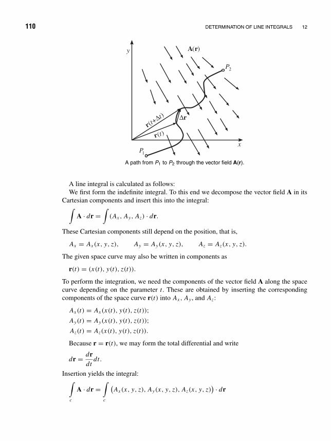
110 DETERMINATION OF LINE INTEGRALS 12
∆r
r( )tr( +
)t
t∆
( )rAy
x
P2
P1
A path from P1 to P2 through the vector field A(r).
A line integral is calculated as follows:We first form the indefinite integral. To this end we decompose the vector field A in its
Cartesian components and insert this into the integral:∫A · dr =
∫(Ax , Ay, Az) · dr.
These Cartesian components still depend on the position, that is,
Ax = Ax (x, y, z), Ay = Ay(x, y, z), Az = Az(x, y, z).
The given space curve may also be written in components as
r(t) = (x(t), y(t), z(t)).
To perform the integration, we need the components of the vector field A along the spacecurve depending on the parameter t . These are obtained by inserting the correspondingcomponents of the space curve r(t) into Ax , Ay , and Az :
Ax (t) = Ax (x(t), y(t), z(t));Ay(t) = Ay(x(t), y(t), z(t));Az(t) = Az(x(t), y(t), z(t)).
Because r = r(t), we may form the total differential and write
dr = drdt
dt.
Insertion yields the integral:∫c
A · dr =∫c
(Ax (x, y, z), Ay(x, y, z), Az(x, y, z)
) · dr

DETERMINATION OF LINE INTEGRALS 111
=∫c
[(Ax (x(t), y(t), z(t)), Ay(x(t), y(t), z(t)), Az(x(t), y(t), z(t))
) · drdt
]dt.
Because of
drdt
=(
dx
dt,
dy
dt,
dz
dt
),
one further has∫c
A · dr =∫ [
Ax (t)dx(t)
dt+ Ay(t)
dy(t)
dt+ Az(t)
dz(t)
dt
]dt.
This integral, as a rule, may be evaluated easily. Insertion of the limits after the integrationyields the wanted line integral.
Example 12.1: Line integral over a vector field
The vector field A and the space curve r = r(t) are given by
A = (3x2 − 6yz, 2y + 3xz, 1 − 4xyz2),
r(t) = (t, t2, t3).
The components of the space curve are
x = t ⇒ x = 1,
y = t2 ⇒ y = 2t,
z = t3 ⇒ z = 3t2.
We now insert∫A · dr =
∫ (Ax
dx
dt+ Ay
dy
dt+ Az
dz
dt
)dt
=∫ [(
3t2 − 6t5) · 1 + (
2t2 + 3t4) · 2t + (
1 − 4t9) · 3t2
]dt.
The integral with the limits t1 = 0 and t2 = 2 is then
2∫0
A · dr = −4064.

13 The Integral Lawsof Gauss andStokes
Gauss Law:1
By means of the concept of divergence worked out in the preceding chapter, one may also
1Carl Friedrich Gauss, b. April 30, 1777, Brunswick—d. Feb. 23, 1855, Gottingen. Gauss was the son of aday laborer and attracted attention very early by his exceptional mathematical talent. The Duke of Brunswicksponsored the costs of his education as of 1791. Gauss studied from 1794–1798 in Gottingen and got his doctoratein 1799 in Helmstedt. As of 1807 Gauss was director of the observatory and professor at the university in Gottingen.He refused all offers to come, for example, to Berlin at the academy. Gauss started his scientific work in 1791with investigations on the geometric-arithmetic mean, on the distribution of prime numbers, and in 1792 on thefoundations of geometry. Already in 1794 he found the least-squares method, and from 1795 dates the intensiveinvestigation of number theory, e.g., with the quadratic reciprocity law. In 1796 Gauss published his first papercontaining the proof that, except for the known cases, regular n-gons may be constructed by means of circle andruler if n is a Fermat prime number. In particular, this applies to the 17-gon. In his dissertation (1799) Gauss gavethe first exact proof of the fundamental law of algebra, which was followed by further ones. From the unpublishedworks it is known that in the same year Gauss already had the foundations of the theory of elliptic and modulefunctions. The first extensive work Gauss published in 1801 is his famous Disquisitiones arithmeticae, which areconsidered as the start of the more recent number theory. There one finds, for example, the theory of quadraticcongruences and the first proof of the quadratic reciprocity theorem, the “theorema aureum,” as well as the theoryof cyclotomy.
Around 1801 Gauss became interested in astronomy. The results of these studies were as follows: In 1801 theorbit calculation of the planet Ceres; in 1809 and 1818 the investigations on secular perturbations; and in 1813 onthe attraction by the general ellipsoid. In 1812 the treatise on the hypergeometric series was published; it containsthe first correct and systematic study of convergence.
As of 1820 Gauss increasingly dealt with geodesy. The most important theoretical achievement is 1827’s theoryof surfaces with the “theorema egregium.” Gauss also pursued practical geometry, he performed very extensivemeasurements in 1821–1825. Despite such costly work, in 1825 and 1831 his papers on biquadratic remaindersappeared. The second of these treatises contains the representation of complex numbers in the plane and a newtheory of prime numbers.
In his last years Gauss also became interested in physical problems. The most important results are 1833–1834’sinvention (together with W. Weber) of the electric telegraph and 1839–1840’s potential theory, which became anew branch of mathematics.
Many important results of Gauss are only known from the diary and the letters. For example, already in 1816Gauss had developed the non-Euclidean geometry. The reason for the attitude not to publish important results isto be seen in the extraordinarily high standard Gauss set also to the form of his works and in the attempt to avoidneedless discussion.
112

GAUSS LAW:2 113
calculate the excess of the outgoing over the incoming vector flow of a vector field Afor an arbitrarily large volume V . For this purpose we decompose this volume into smallvolume elements dV , calculate the divergence for each volume element, and sum up overall volume elements, that is, the total flow is given by a volume integral:
φ =∫V
div A dV .
Because the in- or outgoing vector flow of this volume has to pass across the surfaces F ,it may also be represented by a surface integral
φ =∫F
A · n d F.
The combination of the surface integral with the integral over the volume yields the Gausslaw:∫
V
div A dV =∫F
A · n d F.
This relation clearly states: The sum of the partial flows out of each or into each volumeelement dV , respectively, equals the flow of the vector field A across the surface of thisvolume.
In the interior of the volume, the flows from one volume element into the next onemutually cancel. Hence, when integrating over the volume elements, there remains onlythe flow out of or into the total volume.
div AA
A
A
A( , , )x y z
A( , , )x y z
n
n
The divergence of the vectorfield A describes the sourcesand sinks of A.
The proof of the Gauss theorem may be performed some-what more formally by means of the definition of the diver-gence
div A = limV →0
∫F A · n d F
V= lim
V →0
∫F A · dF
V.
There is∫V
div A dV = limVi →0
∑i
(div A)iVi
= limVi →0
∑i
1
Vi
∫Fi
A · n d FVi
= limVi →0
∑i
∫Fi
A · n d F =∫F
A · n d F.
The in-flows and out-flows at neighboring cells cancel each other, except for those onthe surface.

114 THE INTEGRAL LAWS OF GAUSS AND STOKES 13
z
y
x
A
A
A
Ad ( , , )F x y z
n
V
Illustration of the flow of the vector field A through the volume V . The flow through the surface equalsthe sum of the intensities of sources and sinks within the volume. This is the meaning of the Gausstheorem.
The Gauss theorem:n n
n
a0
0
dΩ
dΩdΩ
F´
F
4
3 1
2
Proofing the Gauss theorem.
Besides the Gauss law we have just encountered,there holds also a theorem for special vector fieldswhich is called the Gauss theorem. Central forcefields, for example, the gravitational field of a masspoint or the electrostatic field of a point charge, areof the form
K = κrr3
, (13.1)
where κ is a coupling constant. For these fields theGauss theorem holds:
Let F be a closed area and r the position vector of an arbitrary point (x, y, z) measuredwith respect to the origin O (center of force).
For the force flow through the area it holds that
∫∫F
K · n d F = κ
∫∫F
n · rr3
d F =
4πκ if O is inside F ,
0 if O is outside F .(13.2)

GEOMETRIC INTERPRETATION OF THE GAUSS THEOREM: 115
The force flow of such a central force through a closed surface about the center of force Ois therefore 4π · intensity κ of the force field. This may be realized as follows: Accordingto the Gauss theorem, it holds that∫∫
F
n · rr3
d F =∫∫∫
V∇ · r
r3dV . (13.3)
But now according to problem 11.5, div r/r3 = 0 everywhere except for r = 0 (i.e., at theorigin). Hence, the second case of equation (13.2) has been demonstrated: If O is outsideF , then div r/r3 = 0 holds everywhere inside the closed surface F .
But if O is within the surface, we form a spherical surface F ′ of radius a around O . Forthe closed volume limited by F and F ′, it then holds that∫∫
F+F ′
n · rr3
d F =∫∫
F
n · rr3
d F +∫∫
F ′
n · rr3
d F =∫∫∫
V −V ′∇ · r
r3dV = 0. (13.4)
Here V − V ′ is the volume enclosed by the surfaces F and F ′. Within V − V ′ againdiv r/r3 = 0 everywhere, as the coordinate origin O lies outside this volume. From (13.4)it now follows that∫∫
F
n · rr3
d F = −∫∫
F ′
n · rr3
d F. (13.5)
On the spherical surface F ′ holds: n = −r/a, where |r| = a, such that
n · rr3
= − (r /a) · ra3
= −r · ra4
= −a2
a4= − 1
a2.
Therefore, for equation (13.5), it holds that∫∫F
n · rr3
d F = −∫∫
F ′
n · rr3
d F = −∫∫
F ′
(− 1
a2
)d F = 4πa2
a2= 4π. (13.6)
This is the first statement of equation (13.2).
Geometric interpretation of the Gauss theorem:
nn
0 1
d =Ω dωr2
dωr
dF
The area of the shadow under central pro-jection of the surface dF on the unit sphereequals the solid angle.
Let d F be a surface element. If the border ofthis surface element is connected with O (seeopposite sketch), there arises a cone.
dω denotes that area cut out of a sphericalsurface with the center O and the radius r bythis cone. The solid angle d determined bythe area d F and the point O is defined by
d = dω
r2(13.7)

116 THE INTEGRAL LAWS OF GAUSS AND STOKES 13
and is numerically identical with the surfacefraction cut out by the cone from a unit sphereof radius 1 centered about O .
The positive normal vector to the area d F is denoted by n. If is the angle between nand r, there results the relation
cos = n · rr
. (13.8)
From there follows the expression
dω = ±d F cos = ±n · rr
d F; (13.9)
thus, one can write for d
d = ±n · rr3
d F. (13.10)
Depending on whether the vectors n and r enclose an acute or obtuse angle, the positive ornegative sign in equations (13.9) and (13.10) is chosen.
Let F be the surface in the figure on page 114 that is characterized by the fact that anystraight line may intersect it in at most two points. If O lies outside F , then, according to(13.10), for the area element 1 the following expression results:
n · rr3
d F = d. (13.11)
Analogously, for the area element 2 it holds that
n · rr3
d F = −d. (13.12)
Integration over these two regions yields the value zero, as their solid angle contributionsmutually compensate. If the integration is now performed over the entire surface F , oneimmediately sees that the integral∫∫
F
n · rr3
d F = 0, (13.13)
because for any positive contribution there exists a corresponding negative contribution.If O now lies within F , then for any of the area elements 3 and 4
n · rr3
d F = d. (13.14)
This now implies that the contributions of the two regions to the surface integral areadding up. Because the total solid angle is identical to the surface of the unit sphere,namely has the value 4π , it follows that∫∫
F
n · rr3
d F = 4π. (13.15)
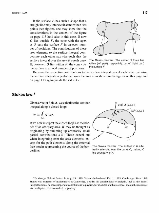
STOKES LAW 117
F
0
0
4
32
1
The Gauss theorem: The center of force lieswithin (left part), respectivly, out of (right part)the surface F .
If the surface F has such a shape that astraight line may intersect it at more than twopoints (see figure), one may show that theconsiderations in the context of the figureon page 113 hold also in this case. If nowO lies outside F , the cone with the apexat O cuts the surface F in an even num-ber of positions. The contributions of thesearea elements to the surface integral com-pensate each other pairwise such that thesurface integral over the area F equals zero.If, however, O lies within F , the cone cutsthe surface in an odd number of positions.
Because the respective contributions to the surface integral cancel each other pairwise,the surface integration performed over the area F as shown in the figures on this page andon page 113 again yields the value 4π .
Stokes law:3
A
n
dr
curl ( , , )A x y z
∆F x y z( , , )
C
The Stokes theorem: The surface F is arbi-trarily extended over the curve C, making Cthe boundary of F .
Given a vector field A, we calculate the contourintegral along a closed loop:
W =∮
CA · dr.
If we now interpret the closed loop s as the bor-der of an arbitrary area, W may be thought asoriginating by summing up arbitrarily smallpartial contributions dW : These cancel outwhen integrating over the area elements, ex-cept for the path elements along the externalfree border representing the course of the bor-derline:
3Sir George Gabriel Stokes, b. Aug. 13, 1819, Skreen (Ireland)—d. Feb. 1, 1903, Cambridge. Since 1849Stokes was professor of mathematics in Cambridge. Besides his contributions to analysis, such as the Stokesintegral formula, he made important contributions to physics, for example, on fluorescence, and on the motion ofviscous liquids. He also worked on geodesy.

118 THE INTEGRAL LAWS OF GAUSS AND STOKES 13
C
C3 C2
C4 C1
A r.d A r.di Ci C
=
Explanation of Stokes theorem: The sum of the contour integrals over the curves Ci yields the contourintegral over the border curve C.
The infinitesimal contributions dW may be represented by the flow of curl A through thearea elements d F , as follows:
Wi = (n · curl A)iFi =∮
CFi
A · drFi
· Fi =∮
CFi
A · dr, (13.16)
where n is the vector pointing perpendicular to the area element d F . We integrate (see alsofigure on this page) and obtain
W =∮
cA · dr =
∑i
∮ci
A · dr =∑
i
(n · curl A)iFi =∫F
n · curl A d F . (13.17)
By inserting the preceding line into the contour integral, one obtains the Stokes law:∮C
A · dr =∫F
n · curl A d F. (13.18)
This may be expressed somewhat less precisely as follows: The sum of vortices over anarea yields the vortex about the border of the area.
Problem 13.1: Path independence of a line integral
Show by means of the Stokes theorem that, assuming A = ∇φ, the line integral from point P1 topoint P2 is independent of the path.
Solution We first form the rotation of the vector field A; because A = ∇φ, we obtain
curl A = curl ∇φ = ∇ × ∇φ = 0.
By inserting this in the Stokes theorem, we obtain∫F
curl A · n d F =∮
A · dr = 0.

STOKES LAW 119
The above relation is fulfilled for arbitrary but closed curves. One has (compare figure):∮C1+C2
A · dr =P2∫
P1C1
A · dr +P1∫
P2C2
A · dr =P2∫
P1C1
A · dr −P2∫
P1C2
A · dr = 0.
y
x
C1
P2
P1
C2
The line integral from P1 to P2does not depend on the path forconservative vector fields (curl A =0). The line integral vanishes forclosed paths.
The line integral is path-independent since the path from P1
to P2 must not coincide with the path from P2 to P1, and never-theless the relation
P2∫P1C1
A · dr −P2∫
P1C2
A · dr = 0
is fulfilled. This may also be proved in an alternative way:
2∫1
∇φ · dr =2∫
1
dφ = φ(2) − φ(1).
Thus, the integral depends only on the function values φ at positions 1 and 2, but not on the specialpath of integration. This discovery is highly important because it allows us to understand for whichforce fields a potential exists.
Additional remark: If A = grad φ ⇒ curl A = 0, because curl grad φ = 0, andtherefore, according to Stokes,
∮A·dr = 0. Inversely, if for arbitrary closed paths
∮A·dr =
0, then it follows from the definition of rotation n · curl A = limF→0(∮
A · dr/F) thatcurl A = 0. From there in turn it follows that A = ∇φ, where φ = ∫ r
r1A(r′)dr′. The
arising integral may then be taken along an arbitrary path from r1 to r (because of the pathindependence of the integral). This important statement shall now be proved:
Given
A(r) with curl A(r) = 0,
if the line integral
φ(r) =r∫
r1
A(r′) · dr′ (13.19)
is independent of the specially selected path, one has
A(r) = ∇φ(r) . (13.20)
Proof: Because the integration contour may be chosen arbitrarily, we adopt especially
(x1, y1, z1)x−→ (x, y1, z1)
y−→ (x, y, z1)z−→ (x, y, z) (see figure),
φ(x, y, z) =r∫
r1
A(r) · dr =r∫
r1
[A1(r) dx + A2(r) dy + A3(r) dz] (13.21)

120 THE INTEGRAL LAWS OF GAUSS AND STOKES 13
=x∫
x1
A1(x ′, y1, z1
)dx ′ +
y∫y1
A2(x, y′, z1
)dy′ +
z∫z1
A3(x, y, z′) dz′.
z
y
x
(x,y,z1)
(x,y1,z1)(x1,y1,z1)
(x,y,z)
A special integration path for cal-culating φ(x , y , z).
For the function φ constructed in this way it holds that
∂φ
∂z= A3(x, y, z),
∂φ
∂y= A2(x, y, z1) +
∫ z
z1
∂ A3(x, y, z′)∂y
dz′
= A2(x, y, z1) +∫ z
z1
∂ A2(x, y, z′)∂z′ dz′.
Here we used curl A = 0, which means for the x-component ∂ A3/∂y = ∂ A2/∂z.
In the following we also employ the vanishing of the other components of curl A = 0:
∂φ
∂y= A2(x, y, z1) + A2(x, y, z′)
∣∣∣∣zz1
= A2(x, y, z)
∂φ
∂x= A1(x, y1, z1) +
∫ y
y1
∂ A2(x, y′, z1)
∂xdy′ +
∫ z
z1
∂ A3(x, y, z′)∂x
dz′
= A1(x, y1, z1) +∫ y
y1
∂ A1(x, y′, z1)
∂y′ dy′ +∫ z
z1
∂ A1(x, y, z′)∂z′ dz′
(because curl A = 0)
= A1(x, y1, z1) + A1(x, y, z1) − A1(x, y1, z1) + A1(x, y, z) − A1(x, y, z1).
The terms cancel each other out pairwise up to one summand, such that it finally remainsthat
∂φ
∂x= A1(x, y, z) .
In total we thus have demonstrated that the function φ(r) defined by the line integralφ(r) = ∫ r
r1A · dr satisfies the equation A = ∇φ . Hence, for a given vector field A
satisfying curl A = 0, one may always calculate the potential function φ(r) by a lineintegral. The function −φ(r) will later be called the potential of the force field A(r)(compare Problem 13.4 and Chapter 17).
This very detailed proof that, with definition 13.21 we have grad φ(r) = A(r), can begiven in a more succinct and elegant way: Because
φ(r + dr) = φ(r) + grad φ · dr,
we find
grad φ · dr = φ(r + dr) − φ(r) =∫ r+dr
rA(r′) · dr′ = A(r) · dr .

STOKES LAW 121
Because this holds for any arbitrary dr, it follows that
grad φ(r) = A(r) .
Problem 13.2: Determination of the potential function
Show for the vector field
A = (2xy + z3, x2 + 2y, 3xz2 − 2)
that∫
A · dr for a path from (1, −1, 1) to (2, 1, 2) is independent of the path. Calculate the value ofthe integral. Find the potential function φ(x, y, z).
Solution One has curl A = 0. We check this, for example, for the x-component: (curl A)x = ∂ Az/∂y −∂ Ay/∂z = 0 − 0 = 0. The other components of curl A will be calculated similarly.
The integral φ(r) = ∫ rr1
A · dr is therefore path-independent, and A = grad φ = ∇φ. Accordingto (13.21), with the arbitrarily and hence effectively choosable r1 = 0, 0, 0 (we sometimes adoptbraces for notation of vectors), we then obtain
φ(x, y, z) =∫ x
0A1(x ′, y1, z1) dx ′ +
∫ y
0A2(x, y′, z1) dy′ +
∫ z
0A3(x, y, z′) dz′
= 0 +∫ y
0(x2 + 2y′) dy′ +
∫ z
0(3xz′2 − 2) dz′
= x2 y′ + y′2∣∣∣∣y
0
+ xz′3 − 2z′∣∣∣∣z0
= x2 y + y2 + xz3 − 2z.
Indeed we easily check
∇φ = (2xy + z3)e1 + (x2 + 2y)e2 + (3z2x − 2)e3.
Because A = ∇φ, the line integral is path-independent. The value of the integral is determined asfollows:∫ (2,1,2)
(1,−1,1)
A · dr =∫ (2,1,2)
(1,−1,1)
∇φ · dr =∫ (2,1,2)
(1,−1,1)
dφ,
= φ(2, 1, 2) − φ(1, −1, 1),
= (4 + 1 + 16 − 4) − (−1 + 1 + 1 − 2) = 18.
Of course, the line integral might be determined also in another way, by integrating, for instance,along an arbitrary contour (an arbitrary curve r(t) between the points 1, −1, 1 and 2, 1, 2).
Problem 13.3: Vortex flow of a force field through a half-sphere
Let A = zxex − (xy −3z)ey + (4yz − x)ez be a given force field. Calculate the flow of curl A throughthe half-sphere above the x, y-plane. (Use spherical coordinates for the integration.)
There are
A = xzex − (xy − 3z)ey + (4yz − x)ez ,
curl A = (4z − 3)ex + (x + 1)ey − yez .

122 THE INTEGRAL LAWS OF GAUSS AND STOKES 13
1. Solution: The upper half-sphere is parametrized by
r = a
⎛⎝ cos ϕ sin ϑ
sin ϕ sin ϑ
cos ϑ
⎞⎠ with 0 ≤ ϕ < 2π, 0 ≤ ϑ ≤ π
2.
The nonnormalized normal vector is
n = ∂r∂ϑ
× ∂r∂ϕ
= · · · = a sin ϑ r.
The area element is given by dF = (∂r/∂ϑ)dϑ × (∂r/∂ϕ)dϕ = n dϑ dϕ.In the new coordinates curl A reads
curl A =⎛⎝ 4a cos ϑ − 3
a cos ϕ sin ϑ + 1
−a sin ϕ sin ϑ
⎞⎠ .
Thereby the integral becomes
I =∫∫
curl A · dF
=∫ π/2
0dϑ
∫ 2π
0dϕ n · curl A
=∫ π/2
0dϑ
∫ 2π
0dϕ a2 sin ϑ
(4a cos ϕ sin ϑ cos ϑ − 3 cos ϕ sin ϑ
+ a sin ϕ cos ϕ sin2 ϑ + sin ϕ sin ϑ − a sin ϕ sin ϑ cos ϑ)
= 0 ,
because∫ 2π
0sin ϕ dϕ =
∫ 2π
0cos ϕ dϕ =
∫ 2π
0sin ϕ cos ϕ dϕ = 0 .
2. Solution: According to the Stokes theorem,
I =∫∫
curl A · dF =∫
CA · dr,
where C is the border of the half-sphere,
r = a
⎛⎝ cos t
sin t
0
⎞⎠ with 0 ≤ t < 2π,
dr = a
⎛⎝− sin t
cos t
0
⎞⎠ dt,
I = −a3
∫ 2π
0dt sin t cos2 t = 0.

STOKES LAW 123
Problem 13.4: On the conservative force field
What is a conservative force field? Is the force field F = (3xz − y)ex − xey +(3/2)x2ez conservative?If yes, determine the potential V and the work A to be performed to move a particle from point (1,1,1) to (2, 2, 2).
Solution One has F = (3xz − y)ex − xey + (3/2)x2ez .A force field F is conservative if it can be represented by F = −∇V . Then it holds that curl F = 0,
because curl(∇V ) ≡ 0.One easily checks that ∇ × F = curl F = 0:
curl F =
∣∣∣∣∣∣∣∣ex ey ez
∂/∂x ∂/∂y ∂/∂z
3xz − y −x 32 x2
∣∣∣∣∣∣∣∣ = 0 .
Thus, it holds that
F = −∇V = −∂V
∂xex − ∂V
∂yey − ∂V
∂zez
= (3xz − y)ex − xey + 3
2x2ez .
Comparison of coefficients yields:
(1)∂V
∂x= −3xz + y; (2)
∂V
∂y= x; (3)
∂V
∂z= −3
2x2.
By integration follows:
(1) V = −3
2x2z + xy + f1(y, z);
(2) V = xy + f2(x, z);
(3) V = −3
2x2z + f3(x, y).
These equations coincide if one chooses
f1(x, y) = c,
f2(x, z) = −3
2x2z + c,
f3(x, y) = xy + c .
From that it follows that
V = −3
2x2z + xy + c .

124 THE INTEGRAL LAWS OF GAUSS AND STOKES 13
Because F is conservative, for the work A we have
A =∫
F · dr = −∫
∇V dr = −∫
dV
⇒ A = −V (2, 2, 2) + V (1, 1, 1)
= −[−3
2x2z + xy + c
](2,2,2)
(1,1,1)
= 71
2.

14 Calculation ofSurface Integrals
Given an area F and a vector field A, we look for the flow of the field through the area.For this purpose we subdivide the area into surface elements Fi and calculate the productA · n · Fi , which represents the flow of the field A through the area element Fi . Heren is the normal vector of magnitude 1 pointing perpendicularly to the area element Fi .We now sum up these products over all i and, by changing to infinitesimal area elements,
z
y
x
x-Coordinate -CoordinateLine
yLine
ne3
e3
dFdF
dxdy
Example of a surface and its shadow areawhen calculating surface integrals.
obtain the surface integral:∫F
A · n d F,
which represents the wanted flow. To calculatethis integral, we convert Fi to Cartesian co-ordinates. The area elements d F are alwayspositive. We therefore set absolute bars:
|n · e3|d F = dx dy
or
d F = dx dy
|n · e3| .
We insert this expression into the surface in-tegral and obtain∫
F
A · n d F =∫F
A · n|n · e3| dx dy .
The surface integral is thereby traced back to a double integral over the shadow area inthe x-y-plane.
125

126 CALCULATION OF SURFACE INTEGRALS 14
One now has to distinguish between two cases:
1. If n is parallel to z, then d F = dx dy, because n · e3 = 1, that is, the projection exactlycorresponds to the prototype.
2. If n is inclined against e3, the projection is smaller than the prototype, that is, d F >
dx dy. In this case n · e3 < 1, and the relation |n · e3| · d F = dx dy is fulfilled.
If the projection of the primordial area onto the x, y-plane (or any other plane) is notunique, such as for areas “hanging over,” uniqueness may always be achieved after someappropriate subdivisions. In such cases the area integral turns into a sum of area integralsover partial areas.
Example 14.1: On the calculation of a surface integral
Given the surface V ≡ 2x + 3y + 6z = 12 (described by the position vector r(x, y) =x, y, (12 − 2x − 3y)/6) and a vector field A = 18z, −12, +3y, find the flow of the fieldthrough the part of this area that is cut out by the three coordinate axes in the first octant.
2
4
6
z
x
y
The y -integral runs from y = 0 to theintersection of the surface with thex , y -plane, i.e., to y = 4 − (2/3)x .
For the calculation, the surface integral is traced back toan integral in the x, y-plane. The integral then takes the form∫
F
A · n|n · e3| dx dy.
We evaluate the individual quantities separately:
n = ∇V (x, y, z)
|∇V | (compare equation (11.6))
= 2, 3, 67
= −−−−→constant.
For n · e3, it therefore results that
n · e3 = 6
7.
To calculate n, one may start also from the position vector r(x, y):
n = rx × ry
|rx × ry | = (1, 0, −2/6) × (0, 1, −3/6)
|(1, 0, −3/6) × (0, 1, −3/6)| = (2/6, 1/2, 1)√49/36
= (2, 3, 6)
7.
For A ·n, it results that A ·n = (36/7)z − (36/7)+ (18/7)y. From there one obtains for the surfaceintegral∫
A · n d F =∫∫ (
36
7z − 36
7+ 18
7y
)7
6dx dy.

CALCULATION OF SURFACE INTEGRALS 127
We replace z by (12 − 2x − 3y)/6 and multiply; then we find for the integral the followingexpression:∫
A · n d F =∫∫
(12 − 2x − 3y + 3y − 6) dx dy
=∫∫
(6 − 2x) dx dy.
To get the limits of the integral, we consider the straight line along which the area V intersects thex, y-plane (z = 0):
2x + 3y = 12; y = 4 − 2
3x .
From there it follows that the y-integration runs between the limits
y = 0 and y = 4 − 2
3x .
The x-integration (integration) of all strips parallel to the y-axis (see figure) is performed betweenthe limits x = 0 and x = 6.
Insertion of the calculated limits yields
∫A · n d F =
6∫x=0
4− 23 x∫
y=0
(6 − 2x) dx dy
=6∫
x=0
(6 − 2x)
⎛⎜⎝ 4− 23 x∫
y=0
dy
⎞⎟⎠ dx
=6∫
x=0
(6 − 2x)
(4 − 2
3x
)dx
=6∫
x=0
(24 − 12x + 4
3x2
)dx
= 24 .
Problem 14.2: Flow through a surface
Given the area F ≡ x2 + y2 = 16 and the vector field A = (z, x, −3y2z) between z = 0 and z = 5,find the flow of the field through the part of the area covering the first octant.
Solution Analogously to the first example, we evaluate n · e2 and A · n; for this end we first determine thenormal vector n:
n = ∇F
|∇F | = (x, y, 0)
4.
For A · n, we get

128 CALCULATION OF SURFACE INTEGRALS 14
A · n = zx
4+ xy
4.
5
F
4
4
0
dz
z
x
y
Illustration of the cylindrical surface F .
We obtain
n · e2 = y
4.
By inserting this into the surface integral, we get∫A · n d F = 1
4
∫∫4(zx + xy)
ydx dz.
We replace y = √16 − x2 and integrate in the limits
from x = 0 to x = 4 or from z = 0 to z = 5 (the shadowarea in the x-z-plane):∫
A · n d F =∫ 4
x=0
∫ 5
z=0
(zx√
16 − x2+ x
)dx dz .
Integration over z yields∫A · n d F =
∫ 4
x=0
(z2
2
x√16 − x2
+ zx
)∣∣∣∣50
dx
=∫ 4
x=0
(1
2
25x√16 − x2
+ 5x
)dx
= −25
2
√16 − x2
∣∣∣∣40
+ 5x2
2
∣∣∣∣40
= 90.
The Mobius strip: The areas in the examples treated so far were orientable, that is, forarbitrary travels over the area the normal vector of the area always remains on one side ofthe area. But there exist nonorientable areas; one example is the Mobius strip.1
In the case of the Mobius strip, there is no outer and inner side, that is, the Mobius striphas only one side. The vector flow through the Mobius strip vanishes; on the contrary, thevector flow through the represented orientable area in general does not vanish.
1August Ferdinand Mobius, b. Nov. 17, 1790, Schulpforta as son of a dance teacher—d. Sept. 26, 1868,Leipzig. Mobius attended the school in Schulpforta and then the university in Leipzig. A donation allowedhim to go on a study trip, leading him among others to Gauss. In 1810 Mobius was appointed director of theobservatory in Leipzig and later also served as a professor at the university. Mobius supported the development ofgeometry by his contributions to the extension of the traditional concept of coordinates, and to the (unconsciously)group-theoretical classification of geometry.

CALCULATION OF SURFACE INTEGRALS 129
CA
DB
n(a)
C
DB
A
(b)
CD
n
n
BA
(c)(a) Orientable surface, (b) Rolled-up strip, and (c) Nonorientable surface (Mobius strip).

15 Volume (Space)Integrals
Let (x, y, z) = (r) be a scalar function of the position, for example, the mass density;the volume integral∫
V dV ≡
∫∫∫V
(x, y, z) dx dy dz = lim∑
k
(rk)Vk (15.1)
then gives the total mass. Vk thereby means small volume cells that in the limit turn overin dxdydz. Volume integrals may be performed also with a vector field F(r) (speakingmore exactly: F(r) is a vector density, and F(r)dV is a vector):∫
VF(r) dV =
∫V
F(x, y, z) dx dy dz = lim∑
k
F(rk)Vk . (15.2)
This corresponds to the sum over all vectors of a vector field F in a volume V , for example,the sum over all forces acting on a rigid body. F(r) is then a force density, and F(r) dV isthe force acting on the volume dV . The mathematical evaluation of a volume integral isperformed according to the following scheme: One constructs a grid consisting of planesparallel to the x, y-, y, z-, and x, z-planes; thus the volume V is subdivided into partialvolumes (cuboids). In this case the triple integral over V may be written as an iterativeintegral of the form∫ b
x=a
∫ g2(x)
y=g1(x)
∫ f2(x,y)
z= f1(x,y)
F(x, y, z) dx dy dz
=∫ b
x=a
∫ g2(x)
y=g1(x)
[∫ f2(x,y)
z= f1(x,y)
F(x, y, z) dz
]dy
dx .
For the given subdivision the innermost integration has to be performed first. This innermostintegration over z corresponds to integrating up columns of cross section dx dy along thez-axis. The lower limit of the columns is given by the area z = f1(x, y), the upper limit byz = f2(x, y). The y-integration then corresponds to summing up these columns in strips
130

VOLUME (SPACE) INTEGRALS 131
parallel to the y-axis. The strips are limited by the function g1(x) and g2(x), respectively.The disks arising this way are integrated along the x-axis by means of the x-integration.
In general, one has to subdivide the volume into larger regions, such that the total tripleintegral may be calculated as sum over partial integrals. We still note that the integrationmay, of course, be performed in an arbitrary sequence. This will now be explained by thefollowing examples.
Example 15.1: Calculation of a volume integral
Let (r) = 45x2 y, and let the volume V be limited by the four planes 4x + 2y + z = 8, x = 0, y =0, z = 0. Calculate
∫(r)dV (see figure).
If means a mass density, then the integral represents the total mass of the volume V . One has
∫V
(r) dV =2∫
x=0
4−2x∫y=0
8−4x−2y∫z=0
(45x2 y) dz dy dx .
z
x
y
8
4
2
SPR
Q
0
∆ ∆ ∆ ∆V x y zk k k k=
Illustration of the integration volume.
Here the integration is performed atfirst over z, then over y, and finally overx . The integration limits are determinedas follows (see figure): z runs for fixedx and y from z = 0 up to the planez = 8 − 4x − 2y. y runs from 0 up tothe straight line y = 4 − 2x in the x, y-plane (cut of the plane 4x + 2y + z = 8with the x, y-plane), and x runs from zeroto 2 (intersection point of the straight liney = 4 − 2x with the x-axis). The calcula-tion now yields
2∫x=0
4−2x∫y=0
8−4x−2y∫z=0
(45x2 y)dz dy dx
= 45
2∫x=0
4−2x∫y=0
x2 y
(z∣∣∣8−4x−2y
0
)dy dx
= 45
2∫x=0
4−2x∫y=0
(x2 y)(8 − 4x − 2y) dy dx
= 45
2∫x=0
[x2(8 − 4x)
(y2
2
∣∣∣∣4−2x
0
)− 2x2
(y3
3
∣∣∣∣4−2x
0
)]dx
= 45
2∫x=0
1
3x2(4 − 2x)3 dx = 128.

132 VOLUME (SPACE) INTEGRALS 15
Problem 15.2: Calculation of a total force from the force density
z
y
x
y=0
0
z x= 2
P
z=4
z=6
R Q S
Illustration of the integration volume.
Integrate the force density f = (2xz, −x, y2)
N/cm3 over the volume V limited by thefive areas x = 0, y = 0, y = 6 cm, z =x2 cm, z = 4 cm (see figure).
Solution The integral∫∫∫V
f(x, y, z) dV
obviously means the total force acting onthe body with this volume. We obtain
2∫x=0
6∫y=0
4∫z=x2
(2xze1 − xe2 + y2e3) dz dy dx
= e1
2∫0
6∫0
4∫z=x2
2xz dz dy dx + e2
2∫0
6∫0
4∫x2
(−x) dz dy dx
+ e3
2∫0
6∫0
4∫x2
y2 dz dy dx
= 128 e1 − 24 e2 + 384 e3 .
The physical dimension of the overall force is, of course,
N
cm3· cm3 = N = Newton.
The unit “Newton” will be explained in the Chapter 17.

PART IINEWTONIAN MECHANICS

16 Newton’s Axioms
The Newtonian1 or classical mechanics is governed by three axioms, which are not inde-pendent of each other:
1. the law of inertia,
2. the fundamental equation of dynamics,
3. the interaction law,
and as a supplement: the theorems on independence concerning the superposition of forcesand of motions.
Premises of Newtonian mechanics are as follows:
1. The absolute time; that means that the time is the same in all coordinate frames, thatis, it is invariant: t = t ′. One may determine in any coordinate frame whether events
1Isaac Newton, b. Jan. 4, 1643, Woolsthorpe (Lincolnshire)—d. March 31, 1727, London. Newton studied in1660 at Trinity College in Cambridge, particularly with the eminent mathematician and theologian L. Barrow.After getting various academic degrees and making a series of essential discoveries, in 1669 Newton becamesuccessor of his teacher in Cambridge. In 1672 he was member and in 1703 president of the Royal Society. From1688 to 1705, he was also member of Parliament, since 1696 attendant and since 1701 mint-master of the Royalmint. Newton’s life’s work comprises, besides theological, alchemistic, and chronological-historical writings,mainly works on optics and on pure and applied mathematics. In his investigations on optics he describes thelight as a flow of corpuscles and by this way interprets the spectrum and the composition of light, as well as theNewton color rings, diffraction phenomena and double-refraction. His main opus Philosophiae Naturalis PrincipiaMathematica (printed in 1687) is fundamental for the evolution of exact sciences. It includes the definition of themost important basic concepts of physics, the three axioms of mechanics of macroscopic bodies, the principleof “actio et reactio,” the gravitational law, the derivation of Kepler’s laws, and the first publication on fluxioncalculus. Newton also dealt with potential theory and with the equilibrium figures of rotating liquids. The ideasfor the great work emerged mainly in 1665–1666 when Newton had left Cambridge because of the pestilence.
In mathematics Newton worked on the theory of series, for example, in 1669 on the binomial series, oninterpolation theory, approximation methods, and the classification of cubic curves and conic sections. ButNewton could not remove logical problems even with his fluxion calculus that was represented in 1704 in detail.His influence on the further development of mathematical sciences can hardly be judged, because Newton dislikedpublishing. When Newton made his fluxion calculus public, his kind of treatment of problems of analysis wasalready obsolete as compared to the calculus of Leibniz. The quarrel over whether Newton or Leibniz deservedpriority for developing the infinitesimal calculus continued until the 20th century. Detailed studies have shownthat they both obtained their results independently of each other [BR].
134

NEWTON’S AXIOMS 135
are simultaneous, because in classical physics one may imagine that signals are beingexchanged with infinitely large velocity.
2. The absolute space; that means that a coordinate frame, being at absolute rest, whichspans the full space, exists. This absolute space may be thought of as being representedby the world ether, which shall be at absolute rest and so to speak embodies the absolutespace. Newton by himself did not believe in the ether; he could imagine the absolute spacealso as being empty. In most recent time the 2.7 Kelvin radiation has been discovered.This radiation is believed to originate from the Big Bang that presumably generated ouruniverse. A coordinate frame in which this radiation is isotropic—of equal intensity inall directions—might also serve as such an absolute coordinate frame.
3. The mass being independent of the velocity.
4. The mass of a closed system of bodies (or mass points) is independent of the processesgoing on in this system, no matter what kind these processes are.
The concepts of absolute time and absolute space, as well as the velocity independence ofthe mass, are lost in the special theory of relativity. Finally, the fourth premise is no longerfulfilled in high-energy processes as, for example, p + p → p + p + π+ + π−. Here newmasses are generated.
Newton formulated his axioms essentially as follows:
Lex prima: Each body remains in its state of rest or uniform rectilinear motion as longas it is not forced by acting forces to change this state.
Lex secunda: The change of motion is proportional to the effect of the driving force andtends toward the direction of that straight line along which the force is acting.
Lex tertia: The action always equals the reaction, or the actions of two bodies onto eachother are always of equal magnitude and of opposite direction.
Lex quarta: Supplement to the laws of motion: Rule of the parallelogram of forces, thatis, forces add up like vectors. Thereby the superposition principle of the actions of forcesis postulated (principle of unperturbed superposition).
Because we deal in the following only with point mechanics, we have to introduce themodel representation of the mass point. Here one abstracts from shape, size, and rotationalmotions of a body and considers only its translational motion. Newton’s axioms in modernform then read as follows:
Axiom 1: Any mass point remains in the state of rest or rectilinear uniform motion untilthis state is terminated by the action of other forces (i.e., by transfer of forces). This is aspecial case of the second axiom. Namely,
F = 0, then m · v = −−−−→constant.
136 NEWTON’S AXIOMS 16
Because of the presupposed velocity independece of the mass, it then holds that
v = −−−−→constant.
If the “quantity of motion” p = m · v is denoted as the linear momentum of the mass point,then the law of inertia is identical with the law of conservation of the linear momentum.
Axiom 2: The first time derivative of the linear momentum p of a mass point is equal tothe force F acting on it:
F = d(m · v)
dt= dp
dt= p,
wherep = mv
is the linear momentum.2.Because in general the mass is a velocity-dependent quantity, that is, it is also time-
dependent, it must not simply be pulled in front of the bracket. In the nonrelativisticNewtonian mechanics (v c ; c = 3 ·108 m s−1), the mass m is, however, treated as beingindependent of the time, and one thus obtains the dynamic fundamental equation:
F = mdvdt
= md2rdt2
= mr = ma.
That means that the acceleration a of a mass point is directly proportional to the force actingon it and coincides with the direction of the force.
If several forces are acting simultaneously onto a mass point, then the above relationaccording to the principle of superposition of forces reads
dpdt
=n∑
i=1
Fi .
Axiom 3: The forces exerted by two mass points onto each other have equal magnitudeand opposite directions; force = – counterforce:
Fi j = −Fj i , where i = j .
Here Fi j is the force exerted by the j th point onto the i th point. Fj i is the force exertedby the i th onto the j th point.
Remark: The relation F = d(mv)/dt is on the one hand a definition of the force, on theother hand a law. The statutory aspect is that, for example, the first time derivative of thelinear momentum occurs, but not the third or fourth or something else. Because the force
2The time derivatives are often abbreviated with a dot, for example d f/dt ≡ f , v = dr/dt = r, or a =d2r/dt2 = r We will use this notation wherever it seems appropriate.

NEWTON’S AXIOMS 137
is the derivative of a vector with respect to a scalar (the time), it is a vector itself. Hence,the addition of forces is governed, for instance, by the law of force parallelogram.
Problem 16.1: Single-rope pulley
e
T
T
W1
W2
A boy and a weight hang-ing at the ends of a rope.
A weight W1 = M1g hangs at the end of a rope. Here, g = 9.81 m/s2
is the gravitational acceleration of all bodies at the surface of the earth.At the other end of the rope, hanging over a roller, a boy of weightW2 = M2g pulls himself upward. Let his acceleration relative to thetightly mounted roller be a. What is the acceleration of the weight W1?
Solution Let b be the acceleration of W1 and T the rope tension. The Newtonianequations of motion then read
(a) For the mass M2 (boy):
−M2 · ae = M2g e − T e; (16.1)
(b) for the mass M1 (weight W1):
M1b e = M1g e − T e. (16.2)
These are two equations with two unknowns (T, b). Their solution may be given immediately:
T = M2(a + g); (16.3)
b = g − T
M1
= g − M2
M1(a + g)
= (M1 − M2)g − M2a
M1. (16.4)
If M1 = M2, it follows that b = −a, as it should be. On the other hand, if a = 0, it follows thatb = (M1−M2)
M1g and vanishes for the case M1 = M2, as expected.
Problem 16.2: Double-rope pulley
A mass M1 hangs at one end of a rope that is led over a roller A (compare the figure). The other endcarries a second roller of mass M2, which in turn carries a rope with the masses m1 and m2 fixed toits ends. The gravitational force is acting on all masses. Calculate the acceleration of the masses m1
and m2, as well as the tensions T1 and T in the ropes.

138 NEWTON’S AXIOMS 16
e
T
T1
T
T1
M 1
m1
M 2
m2
A
Masses and forces at the double-rope pulley.
Solution We introduce the unit vector e ⊥ pointing upward (see figure)and denote the string tensions by T = T e and T1 = T1e,respectively (see figure). The individual masses are influ-enced by the string tension (i.e., the force in the rope) andby the gravitational force. We now write down the equationsof motion for the individual masses according to Newton’sfundamental law.
M1a1e = −M1ge + T e ,
−M2a1e = −M2ge + T e − 2T1e ,
m1(a2 − a1)e = −m1ge + T1e ,
m2(−a2 − a1)e = −m2ge + T1e . (16.5)
The acceleration of the mass M1 has been denoted by a1e,that of the mass M2 is then (because of the constant ropelength) −a1e; the acceleration of the mass m1 relative to themass M2 is a2e, that of the mass m2 is −a2e. 16.5 representsa set of four equations with the four unknowns: a1, a2, T, T1.Subtraction of the second equation from the first one yields
(M1 + M2)a1 = −(M1 − M2)g + 2T1 . (16.6)
The addition of the last two equations of 16.5 leads to
−(m1 + m2)a1 + (m1 − m2)a2 = −(m1 + m2)g + 2T1 . (16.7)
The subtraction of 16.7 from 16.6 then yields a relation between a1 and a2:
(M1 + M2 + m1 + m2)a1 − (m1 − m2)a2 = (−M1 + M2 + m1 + m2)g . (16.8)
A second relation of this kind is obtained by subtracting the last two equations 16.5 from eachother, namely
−(m1 − m2)a1 + (m1 + m2)a2 = −(m1 − m2)g . (16.9)
The accelerations a1 and a2 are now found from equations 16.8 and 16.9:
a1 = −M1(m1 + m2) + M2(m1 + m2) + 4m1m2
(m1 + m2)(M1 + M2) + 4m1m2g; (16.10)
a2 = −2M1(m1 − m2)
(m1 + m2)(M1 + M2) + 4m1m2g, (16.11)
such that the total acceleration of mass m1 is obtained as
a2 − a1 = −M1m1 + 3M1m2 − M2(m1 + m2) − 4m1m2
(m1 + m2)(M1 + M2) + 4m1m2g (16.12)
and that of mass m2 is
(−a2 − a1) = M1(3m1 − m2) − M2(m1 + m2) − 4m1m2
(m1 + m2)(M1 + M2) + 4m1m2g . (16.13)

NEWTON’S AXIOMS 139
If all masses were identical (M1 = M2 = m1 = m2), then
a2 − a1 = −1
2g, a2 = 0,
and
−a2 − a1 = −1
2g, a1 = 1
2g, (16.14)
as one would expect. The string tension T1 follows with 16.10 from equation 16.6 after a simplecalculation as
T1 = 1
2(M1 + M2)a1 + 1
2(M1 − M2)g
= 4m1m2 M1
(m1 + m2)(M1 + M2) + 4m1m2g. (16.15)
The rope tension T is obtained from the first two equations 16.5, using 16.10 and 16.15, as
T = (M1 − M2)a1
2+ (M1 + M2)g
2+ T1
= M1a1 + M1g = M1(a1 + g)
= 2(m1 + m2)M1 M2 + 8m1m2 M1
(m1 + m2)(M1 + M2) + 4m1m2g. (16.16)
According to 16.15 the rope tension T1 vanishes if one of the masses m1, m2, M1 vanishes. In thiscase the rope is rolling without tension, as is clearly expected. The rope tension T vanishes if eitherM1 = 0, or M2 and one of the masses m1 or m2 (or both) vanish. If m1 = m2 = m = 0 and if M1 = 0,M2 = 0, a limit m → 0 can be taken:
T = 2M1 M2
M1 + M2g.
This is the rope tension in the case of the single roller with the two masses M1 and M2 at the ropeends.

17 Basic Conceptsof Mechanics
Inertial systems
–
z
x
y
P z´
rr
x´ 0´ y´
0
Rr r
=´
The point P in relation to the coordi-nate systems x , y , z and x ′, y ′, z ′.
We ask for the forces acting on a mass point P , as seenfrom two coordinate frames x , y, z and x ′, y′, z′ thatare moving relative to each other, with correspondinglyconvected observers 0 and 0′, respectively. Let r and r′be the position vectors of P in x , y, z and in x ′, y′, z′,respectively. One then obtains the position vector from0 to 0′ as the difference r − r′ = R.
According to Newton’s basic equation:
F = md2rdt2
and F′ = md2r′
dt2. (17.1)
The difference of the observed forces is
F − F′ = md2
dt2(r − r′) = m
d2Rdt2
. (17.2)
Because m = 0, this difference vanishes then and only then if
d2Rdt2
= 0 ordRdt
= −−−−→constant = vR . (17.3)
This means that the forces are then equal if the two coordinate frames are moving withconstant velocity vR relative to each other. Such systems are called inertial systems if one ofthem—and thus all of them—fulfills Newton’s axioms. The statement that in such inertialsystems the Newtonian equations (17.1) have the same form and the forces are also thesame (F = F′) is called the classical relativity principle.
140

WORK 141
Measurement of masses
Masses are measured by comparison with an arbitrarily defined unit mass. If there are threedistinct masses m1, m2, and m3, with m1 representing the unit mass, one may determineexperimentally, for example, m3, starting from the second and third Newton laws, as thequotient of the accelerations:
a1
m1
a3
m3
Central collision.
m1 m3
Noncentral collision.
m1dv1
dt= −m3
dv3
dt, m1 a1 = −m3 a3,
force = −counterforce.
From there it follows that
m3 = m1|a1||a3| ,
where m1 is the unit mass, and a1 and a3 may be determined. Thus,m3 may be measured in units of m1. In the processof measurement (collision) the basic laws (second and third Newtonian laws) are employed.
Correspondingly, it then also holds that
m2 = m1|a1||a2| . (17.4)
Work
M
P1
P2
FC
ϕdr
The work integral.
A force F causes a displacement of a mass point M by an infinites-imally small path element dr and thereby performs the work dWthat is defined as follows:
dW = F · dr = |F||dr| cos(F, dr).
The unit of this scalar is therefore
g cm2
s2= 1 erg or
kg m2
s2= 1 Nm ⇒ 1 erg = 10−7 Nm.
Here 1 Newton (N) = kg m/s2 is the unit of force.The total work W needed to move M along a curve C between the points P1 and P2 is
given by the following line integral:
W =∫C
F · dr =P2∫
P1
F · dr . (17.5)

142 BASIC CONCEPTS OF MECHANICS 17
Power is work performed per unit time:
dW
dt= F · dr
dt= F · v. (17.6)
The unit of power is[g cm2/s3 = erg/s
]or[kg m2/s3 = Nm/s
].
Kinetic energy
In order to accelerate a mass point and to bring it to a definite velocity, work must beperformed. This work is then stored in the mass point in the form of kinetic energy. Wetherefore start from the integral of work:
W =r2∫
t1
F · dr =r2∫
t1
F · v dt
=t2∫
t1
mdvdt
· v dt = 1
2m
v2∫v1
d(v · v)
= 1
2m(v2
2 − v21) = T2 − T1 ,
T = 1
2mv2 = kin. energy. (17.7)
Conservative forces
A force is called conservative if the force field F may be represented by
F = − grad V (x, y, z) (definition). (17.8)
If this is true, then the work integrals are path-independent:
P2∫P1
F · dr = −P2∫
P1
grad V · dr = −P2∫
P1
dV (see total differential; Chapter 11)
= V (P1) − V (P2) ≡ V1 − V2
= −(V2 − V1). (17.9)
Hence one has
W = V1 − V2 ,

POTENTIAL 143
where V is a scalar field that associates a numerical value to each space point. W is thereforepath-independent. But this further means that for an integration along a closed curve thetotal work must vanish:∮
CF · dr = 0 (17.10)
for conservative forces. An equivalent requirement for conservative forces is
curl F = ∇ × F = 0 .
Indeed we can also conclude this immediately from equation (17.8) since
curl grad V (r) = 0.
Potential
If F(r) = −∇V (r), then the scalar quantity V (x, y, z) is called potential energy, scalarpotential, or, briefly, potential:
V (x, y, z) = −(x,y,z)∫
(x0,y0,z0)
F · dr . (17.11)
Example 17.1: Potential energy
P1
P2
x y z0 0 0
Calculation of the potential en-ergy difference between in thepoints P1 and P2.
Calculation of the potential energy between two points looks like
W =P2∫
P1
F · dr
=(x0,y0,z0)∫
P1
F · dr +P2∫
(x0,y0,z0)
F · dr.
The presupposition is a conservative force field, and thus path-independence of the work integral.
W = −P1∫
(x0,y0,z0)
F · dr +P2∫
(x0,y0,z0)
F · dr = V (x1 y1z1) − V (x2 y2z2).
Therefore, the work represents a potential difference that is independent of the choice of the referencepoint. The potential itself is always defined relative to a reference point (x0, y0, z0) and is thereforeundetermined by an additive constant. The zero point of the potential may be set arbitrarily. Thisarbitrariness corresponds to the (arbitrary) additive constant in the potential.

144 BASIC CONCEPTS OF MECHANICS 17
Energy law
On deriving the kinetic energy, we found the following relation for the work:
W = T2 − T1.
For conservative fields there also holds the other relation between the same points P1
and P2:
W = V1 − V2.
This implies
T2 + V2 = T1 + V1. (17.12)
This is the energy conservation law (briefly: energy law), where T + V = E representsthe total energy of the mass point.
Written out in detail, the energy conservation law reads
1
2mv 2
2 +(
−∫ P2
P0
F · dr)
= 1
2m v 2
1 +(
−∫ P1
P0
F · dr)
(17.13)
or1
2m v 2
2 + V2 = 1
2m v 2
1 + V1
orE2 = E1 .
The premises for this energy conservation law for the motion of a mass point are
1. The basic assumptions and basic laws of the Newtonian mechanics (e.g., nonrelativistictreatment of the mass);
2. conservative force fields, that is, the forces may be written as the negative gradient ofa potential. For force fields that are constant in time, it then holds that E = T + V =constant.
Equivalence of impulse of force and momentum change
If a mass point is affected by a force over a time interval t = t2 − t1, the time integral overthis force is called impulse of force:
t2∫t1
F(t) dt = impulse of force. (17.14)
The impulse of force is equivalent to the momentum change or momentum difference. Thisis seen as follows:

EQUIVALENCE OF IMPULSE OF FORCE AND MOMENTUM CHANGE 145
From the definition of the linear momentum p = mv and from the second Newtonianfundamental equation, it follows that
t2∫t1
F dt =t2∫
t1
d
dt(m v) dt =
t2∫t1
d(m v) = mv2 − mv1 = p2 − p1. (17.15)
m
m
p v1 1= m
p v2 2= m p p2 1– = .F ∆t
F. ∆t
p1
Situation before (top) and after (bottom) theimpulse of force.
Thus a force acting on the mass causes achange of momentum: That is, only of its mag-nitude if F points along p1, and a change ofboth magnitude and direction if F points in anarbitrary angle relative to p1.
If the force F acts during the time t ,the corresponding difference in momentumis Ft = p2 − p1. After the collision, themass moves on a straight line with linear mo-mentum p2.
Problem 17.2: Impulse of momentum by a time-dependent force field
F( )t1
F( )t2
Force field at different times t1 and t2: homogenous(equal at every point in space) at any time, but vari-able with time. For a fixed moment t in time we havecurl F(t) = 0, because F(t) is constant in space. There-fore, we have a time-dependent potential.
A particle of mass m = 2 g moves in thetime-dependent uniform force field:
F =(
24t2
s2, 3
t
s− 16, −12
t
s
)dyn.
The initial conditions are
r(t=0) = r0 = (3, −1, 4) cm
and
v(t=0) = v0 = (6, 15, −8)cm
s.
Here we make use of the units of force
1 dyn = gcm
s2= 10−5 N and 1 N = 1 Newton = 1kg
m
s2.
Find the following quantities:
1. The kinetic energy at the time t = 1 s and t = 2 s.
2. The work performed by the field to move the particle from r1 = r(t=1 s) to r2 = r(t=2 s).
3. The linear momentum of the particle at r1 and r2.
4. The momentum transferred by the field to the particle over the time interval t = 1 s until t = 2 s.

146 BASIC CONCEPTS OF MECHANICS 17
Solution
To 1: v is obtained from F = ma = m(dv/dt) as
v =∫
dv =∫
Fm
dt + v0.
Using the data of the problem, we get for v
v(t) =(
4t3
s3,
3
4
t2
s2− 8
t
s, −3
t2
s2
)cm
s+ (6, 15, −8)
cm
s
and
v(t=1 s) = (10, 7 3
4 , −11) cm
s,
v(t=2 s) = (38, 2, −20)cm
s.
From there we get for the energy
T = 1
2m v 2 = 1
2m v2,
T1 = 281 erg , T2 = 1848 erg .
To 2: The work performed by the field equals the difference of the kinetic energies:
W = T2 − T1 = 1567 erg.
To 3: The momentum of the particle is p = mv:
p1 = (20, 15 1
2 , −22)
gcm
s,
p2 = (76, 4, −40) gcm
s.
To 4: The momentum transferred by the field is obtained from the difference of momenta p2 and p1:
p = p2 − p1 = (56, −11 1
2 , −18)
gcm
s.
Problem 17.3: Impulse of force
A railway carriage of mass m = 18000 kg starts from a roll-off plateau of height 3 m. What is thechange of momentum of the carriage, and which mean force is acting on it when colliding onto abuffer at the bottom of the hill, if the carriage within 0.2 s
(a) Comes to rest ?
(b) Is pushed back to a height of 0.5 m?
Discuss the momentum conservation.

EQUIVALENCE OF IMPULSE OF FORCE AND MOMENTUM CHANGE 147
Solution At the moment of impact the carriage has a momentum p1 that results from the potential energy atthe start from the roll-off plateau:
1
2m v2
1 = mgh ⇒ p1 = m v1 = m(2gh)1/2e1 .
In case (a) the momentum p2 after the impact equals zero; hence
p = p1 − p2 = m(2gh)1/2e1
= 138 096.5 m kg s−1 · e1;the mean force acting over t = 0.2 s is then
F = pt
= 690 482.4 N.
In case (b) the momentum p2 is given by
p2 = m v2 = −m(2gh′)1/2e1,
where h′ is the height regained in the bouncing-back. The momentum change is then
p = p1 − p2 = me1
[(2gh)1/2 + (2gh′)1/2
]= 194 474.1 m kg s−1 e1;
for the mean force we obtain
F = pt
= 972 370.7 N.
The carriage alone does not represent a closed system: The reactive force imposed by the tightlymounted buffer is an external force; therefore, the momentum cannot be conserved.
Problem 17.4: The ballistic pendulum
mG
l
mK y
h
θ θ
m mG K+
Ballistic pendulum and bullet.
The velocity of a bullet may be measured bymeans of the ballistic pendulum. This deviceconsists of a string with negligible weight and aweight of mass mG fixed to the string. The bullet(mass mK , velocity vK ) is shot into the block,where it gets stuck. The arc length s covered bythe center of the mass mG is measured.
(a) Determine the velocity of the block vG afterthe collision, and
(b) Determine the velocity of the bullet vK ifthe following quantities are specified: mG =4 kg, l = 1.62 m, mK = 0.055 kg, s =6.5 cm.
Solution (a) From the momentum conservation law, it follows that
mK vK = (mG + mK )vG (17.16)

148 BASIC CONCEPTS OF MECHANICS 17
and from there for the velocity vG of the block just after the collision
vG = mK
mG + mK· vK . (17.17)
For the kinetic energy it results immediately that
T = 1
2(mG + mK ) · v2
G = mK
mG + mK
(1
2mK v2
K
). (17.18)
This energy coincides with the kinetic energy of the bullet reduced by the factor mK /(mG + mK ).One may wonder why the kinetic energy of the block differs from the kinetic energy 1
2 mK v2K of the
bullet? Where is the energy lost,
E = 1
2mK v2
K − mK
mG + mK
(1
2mK v2
K
)= mG
mG + mK
(1
2mK v2
K
)?
Obviously it must correspond to the heat released by the bullet getting stuck in the block. FormG mK , almost the total energy of the bullet is converted to heat.
Another point is worth being mentioned: On calculating the velocity vG of the block, we startedfrom the momentum conservation law 17.16 but not, as might be thought first, from the energyconservation law ( 1
2 mK v2K = 1
2 (mK + mG)v2G). Which of these two possibilities is now correct?
The puzzle of two seemingly existing possibilities originates from the incomplete formulation ofthe problem. Actually, the percent fraction of the energy converted to heat ought to be specified inaddition. Without any knowledge of this fraction we may, however, argue as follows: We know byexperience that in the process of the bullet getting stuck, no small particles of the block (smallestpieces, molecules) are flying off, but rather the block moves as an entity. The block itself also becomesheated up by the friction of the bullet. In any case, the momentum conservation law must hold strictly,because the heat as a disordered molecular motion on the average does not carry off momentum, butfor sure dissipates energy. In other words: Because the momentum conservation law 17.16 is strictlyfulfilled, we actually may imagine that the energy loss E has been converted to heat. If we hadstrictly required energy conservation without any production of heat, 1
2 mK v2K = 1
2 (mG +mG)v2G ; this
would imply a momentum loss, about which we would have no idea how it might evolve.(b) From the figure in the context of the problem, we get for the height of lift of the block
h = l(1 − cos θ) = 2l sin2 θ
2(17.19)
and in the limit of small displacements θ
h = 2l
(θ
2
)2
= 2l( y
2l
)2 = y2
2l, (17.20)
where sin θ = y/ l and sin θ = θ.
The change of the potential energy of the block after being hit by the bullet is—at maximalelongation of the pendulum—according to the energy conservation law:
V = g(mG + mK )h = T = mK
(mK + mG)
(1
2mK v2
K
). (17.21)
From equations 17.20 and 17.21, we then obtain
gh = m2K
2(mG + mK )2v2
K = gy2
2l. (17.22)

ANGULAR MOMENTUM AND TORQUE 149
In the approximation mK + mG ≈ mG , the velocity vK of the bullet is given by
vK = mG
mKy
√g
l. (17.23)
Insertion of the data given in the formulation of the problem yields
vK = 4
0.055· 6.5 · 10−2
√9.81
1.62= 11.6
m
s.
Angular momentum and torque
y
x
mp
r
L r p=
The definition of angularmomentum: L = r × p.
Angular momentum and torque are always defined with respectto a fixed point, the pivot. If r is the vector from this point to themass point, then the angular momentum is given by
L = r × p. (17.24)
If we put the coordinate frame into the reference point, thenr is the position vector of the mass point, and p is its linearmomentum.
L is an axial vector. L defines an axis through the pivot,the rotational axis, which points perpendicularly to the planespanned by r and p.
Fy
x
m
r
D F= r
The definition of torque:D = r × F.
The corresponding definition holds for the moment of the force,which is defined by
D = r × F, (17.25)
and is also called torque. The time variation of the angular mo-mentum is equal to the torque:
L = D,
because
L = dLdt
= d
dt(r × mv) = dr
dt× mv + r × d(mv)
dt
= v × mv + r × dpdt
= r × F, (17.26)
because v × mv = 0.
The torque of the acting force (r × F) is equal to the time variation of the angularmomentum.
If, in particular, D = r × F = 0 = L, it then follows that L = −−−−−→constant . This is the
conservation law for the angular momentum. But the quantity r × F vanishes only then(except for the trivial cases r = 0, F = 0) if r and F point along the same or the opposite

150 BASIC CONCEPTS OF MECHANICS 17
direction. A force that acts exclusively parallel or antiparallel to the position vector is calledthe central force.
This implies that central forces obey the
Conservation law of angular momentum
L = −−−−−→constant , because D = 0.
Law of conservation of the linear momentum
As long as no forces are acting, the linear momentum p is a constant quantity. In general,
F = d(mv)
dt= m
dvdt
;
and therefore it follows for F = 0 that
mdvdt
= 0.
From there again we get
mv = p = −−−−→constant.
The momentum conservation law is identical to Newton’s Lex prima.
Summary
The premises of the conservation laws concerning the energy, angular momentum, and linearmomentum for a mass point in the Newtonian mechanics (compare to the introduction) are
(a) Energy conservation: If the forces acting on a mass point are conservative (gradientfield: F = −∇V ), then the total energy E = T + V of the mass point is conserved.
(b) Angular momentum conservation: The total angular momentum L is constant intime if the applied (external) torque vanishes, that is, if one is dealing with central forcefields (r × F = 0).
(c) Momentum conservation: If the total external force equals zero then the total linearmomentum is conserved (equivalent to Newton’s Lex prima).

CONSERVATION OF ORIENTATION 151
The law of areas
(See also Chapter 26 on planetary motions; in particular, the Kepler laws.) The premisesand contents of the three conservation laws (total energy, linear momentum, angular mo-mentum) have been formulated already. The angular momentum conservation holds only incentral force fields, as arise, for example, in planetary motion. Conservation of the angularmomentum means constancy of its orientation as well as its magnitude.
Conservation of orientation
Conservation of L = r×p means that the plane spanned by r and p remains fixed in spatialorientation; hence the motion proceeds in a plane.
dFdrr
The area dF = 12 |r × dr|
spanned by the vectors rand dr.
Conservation of the magnitude of the angular momentum isoften denoted as law of areas. The area covered by the “radiusvector” r during the time element dt is
d F = 1
2|r × dr | = 1
2|r × v | dt .
With L = r × p = r × mv = m(r × v), it holds that
d F = 1
2m|L| dt or
d F
dt= 1
2m|L| ,
where d F/dt is the area velocity of the radius vector (area covered per unit time). For theplanetary motion, the law of areas is identical to the second Kepler law:
The radius vector of a planet covers equal areas in equal times.
The law of areas follows directly from the angular momentum conservation law and
rM
Sun
mPlanet
Illustration of the law of equal areas.
holds generally for arbitrary central fields, that is,also for the gravitational force, which is a centralforce with the sun as center. In the perihelion (clos-est distance to sun) the planet is moving faster thanin the aphelion (largest distance to sun).
The situation in the example of Problem 17.5 issimilar: The area velocity is constant, and hencethe velocity v at r = ±b is maximum; at r = ±ait is minimum.
Example 17.5: Forces in the motion on an ellipse
We calculate the force to be applied to a mass point of constant mass to get it moving along the ellipse
r = a cos ωt e1 + b sin ωt e2 .

152 BASIC CONCEPTS OF MECHANICS 17
It is easy to verify from this parameterization the normal form of the equation of an ellipse (see alsoChapter 26),
x2
a2+ y2
b2= 1.
Starting from the second Newtonian axiom, the following ansatz results:
F = mdvdt
= md2rdt2
= md2
dt2(a cos ωt e1 + b sin ωt e2)
= −mω2 [(a cos ωt) e1 + (b sin ωt) e2]
= −mω2r.
The force acts opposite to the direction of the position vector; it is an attractive central force. Theforce center lies at the midpoint of the ellipse.
Such forces that increase linearly with the distance play an important role, for example, for thespring (Hooke’s law – see Section 18) and between the quarks, the primordial constituents of protons,neutrons, and mesons.
The planets also move around the sun along elliptic orbits. The sun as the center of attraction islocated in one of the focal points of the ellipse. As we will see later in Chapter 26, the force acting is
FG = −γmM
r 2
rr
,
that is, the gravitational force between the sun (mass M) and the planet (mass m).We show that this force field is conservative. A necessary and sufficient condition for this property
is the vanishing of the rotation of the force:
curl F = 0,
curl F = −mω2 curl r; hence it suffices to calculate the rotation of r:
curl r =
∣∣∣∣∣∣∣∣∣e1 e2 e3
∂
∂x
∂
∂y
∂
∂zx y z
∣∣∣∣∣∣∣∣∣= e1
(∂z
∂y− ∂y
∂z
)+ e2
(∂x
∂z− ∂z
∂x
)+ e3
(∂y
∂x− ∂x
∂y
)= 0,
namely, the rotation of the position vector vanishes.
y
xA
P
a
b r
Illustration of elliptic motion.
Calculation of the potential at a point P (at the position r)with respect to the zero of the potential at point A (at theposition a): We take a fixed point A on the ellipse (see sketch)and calculate the potential difference between A and the points ofthe trajectory given by r.
V (x, y, z) = −r∫
a
F · dr = mω2
r∫a
r · dr

CONSERVATION OF ORIENTATION 153
= 1
2mω2
r∫a
d(r · r)
= 1
2mω2r 2
∣∣∣∣ra
= 1
2mω2(r 2 − a 2).
With r 2 = r 2, it results that
V (x, y, z) = 1
2mω2(r 2 − a2).
For r = a, one has V (a) = 0, as it should be.
Calculation of the kinetic energy: The velocity is
v = r = (−ωa sin ωt)e1 + (ωb cos ωt)e2 ,
|v| =√
ω2a2 sin2 ωt + ω2b2 cos2 ωt = v ,
T = 1
2mv2 = 1
2mω2
(a2 sin2 ωt + b2 cos2 ωt
).
The kinetic energy is always positive and nonzero, as it must be in this case, to keep the mass pointon the trajectory.
Calculation of the total energy: The total energy is the sum of E = T + V . By inserting thederived relations for T and V , we get
E = 1
2mω2
[a2(sin2 ωt + cos2 ωt
)+ b2(cos2 ωt + sin2 ωt
)− a2]
= 1
2mω2
(a2 + b2 − a2
)= 1
2mω2b2 = constant,
that is, the total energy is time-independent. The distinction of the half-axis b stems from our choice ofreferring the potential energy to the point (x = a, y = 0). For r = ±a the total energy is exclusivelykinetic energy; for r = ±b the kinetic energy is maximum, the potental energy is minimum, namely
V (b) = 1
2mω2(b2 − a2).
Problem 17.6: Calculation of angular momentum and torque
Find the torque D and the angular momentum L with respect to the origin for a mass point m movingon the trajectory r = (a cos ωt, b sin ωt).
Solution r = (a cos ωt, b sin ωt) where a, b = constant
L = r × p = r × mv = m(r × v),
v = r = (−aω sin ωt, bω cos ωt),

154 BASIC CONCEPTS OF MECHANICS 17
L =
∣∣∣∣∣∣∣∣e1 e2 e3
a cos ωt b sin ωt 0
−aω sin ωt +bω cos ωt 0
∣∣∣∣∣∣∣∣ · m
= me3(ab ω cos2 ωt + ab ω sin2 ωt)
= ab ω me3,
that is, L is time-independent, because L = −−−−−→constant . From there it follows that
D = L = 0.
Hence, the force must be a central force. The mass point moves along an ellipse with the half-axesa and b, because
x = a cos ωt, y = b sin ωt,
and, therefore,
x2
a2+ y2
b2= cos2 ωt + sin2 ωt = 1.
Problem 17.7: Show that the given force field is conservative
Show that the following force field is conservative:
F = (y2z3 − 6 xz2)e1 + 2xyz3e3 + (3xy2z2 − 6x2z)e3 .
Solution One has to show that curl F = 0:
curl F =
∣∣∣∣∣∣∣∣∣e1 e2 e3
∂
∂x
∂
∂y
∂
∂zy2z3 − 6xz2 2xyz3 3xy2z2 − 6x2z
∣∣∣∣∣∣∣∣∣= e1
[∂
∂y
(3xy2z2 − 6x2z
)− ∂
∂z
(2xyz3
)]
+ e2
[∂
∂z
(y2z3 − 6xz2
)− ∂
∂x
(3xy2z2 − 6x2z
)]
+ e3
[∂
∂x
(2xyz3
)− ∂
∂y
(y2z3 − 6xz2
)]= e1
(6xyz2 − 6xyz2
) + e2
[(3y2z2 − 12xz
)− (3y2z2 − 12xz
)] + e3
(2yz3 − 2yz3
)= 0,
that is, F is a conservative force field.

CONSERVATION OF ORIENTATION 155
Problem 17.8: Force field, potential, total energy
(a) Show that F = ηr 3r is conservative.
(b) Calculate the potential of a mass point in this field.
(c) What is the total energy of the mass point?
Solution (a)
curl F = ∇ × F
= −η[e1
[3zy
(x2 + y2 + z2
)1/2 − 3zy(x2 + y2 + z2
)1/2]
+ e2
[3xz
(x2 + y2 + z2
)1/2 − 3xz(x2 + y2 + z2
)1/2]
+ e3
[3xy
(x2 + y2 + z2
)1/2 − 3xy(x2 + y2 + z2
)1/2]]
= 0,
where |r| = √x2 + y2 + z2 and |r|3 = r 3 = (x2 + y2 + z2)3/2 have been used.
(b) Potential:
V =r∫
r0=0
F · dr = η
r∫r0=0
r 3r · dr = η
r∫r0=0
r 4dr = ηr 5
5,
with r · dr = 12 d(r · r) = 1
2 d(r 2) = 12 d(r 2) = r dr.
(c) Because the force field is conservative, the energy law E = T + V = constant holds:
T = 1
2mr 2; V (r) = 1
5ηr 5.
It then follows that
E = 1
2mr 2 + 1
5ηr 5.
Problem 17.9: Momentum and force at a ram pile
A crane lifts a mass of weight 1000 kg by 8.5 m upward. Afterward the weight falls onto a ram pile.
(a) Determine the transferred momentum.
(b) Determine the force acting onto the pile if the time of the impulse is 1/100 s.
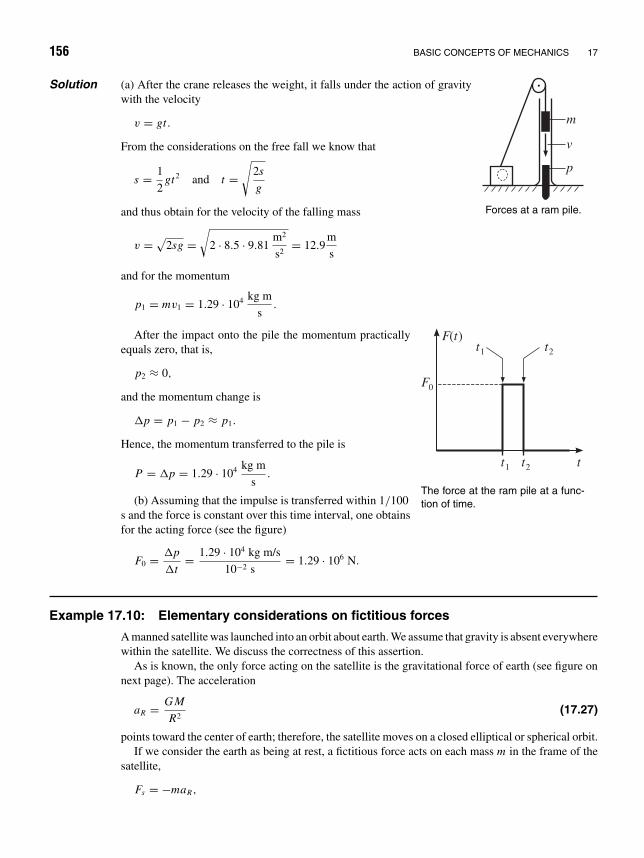
156 BASIC CONCEPTS OF MECHANICS 17
m
v
p
Forces at a ram pile.
Solution (a) After the crane releases the weight, it falls under the action of gravitywith the velocity
v = gt.
From the considerations on the free fall we know that
s = 1
2gt2 and t =
√2s
g
and thus obtain for the velocity of the falling mass
v = √2sg =
√2 · 8.5 · 9.81
m2
s2= 12.9
m
s
and for the momentum
p1 = mv1 = 1.29 · 104 kg m
s.
F t( )
F0
t1
t1
t2
t2
t
The force at the ram pile at a func-tion of time.
After the impact onto the pile the momentum practicallyequals zero, that is,
p2 ≈ 0,
and the momentum change is
p = p1 − p2 ≈ p1.
Hence, the momentum transferred to the pile is
P = p = 1.29 · 104 kg m
s.
(b) Assuming that the impulse is transferred within 1/100s and the force is constant over this time interval, one obtainsfor the acting force (see the figure)
F0 = p
t= 1.29 · 104 kg m/s
10−2 s= 1.29 · 106 N.
Example 17.10: Elementary considerations on fictitious forces
A manned satellite was launched into an orbit about earth. We assume that gravity is absent everywherewithin the satellite. We discuss the correctness of this assertion.
As is known, the only force acting on the satellite is the gravitational force of earth (see figure onnext page). The acceleration
aR = G M
R2(17.27)
points toward the center of earth; therefore, the satellite moves on a closed elliptical or spherical orbit.If we consider the earth as being at rest, a fictitious force acts on each mass m in the frame of the
satellite,
Fs = −maR,
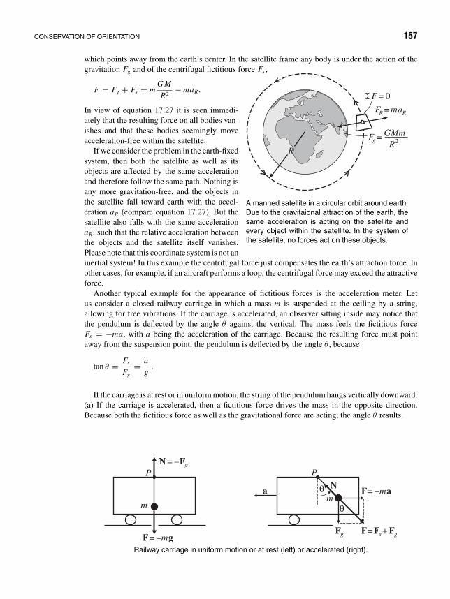
CONSERVATION OF ORIENTATION 157
which points away from the earth’s center. In the satellite frame any body is under the action of thegravitation Fg and of the centrifugal fictitious force Fs ,
R
Fg=
F = 0
F maR R=
GMmR2
A manned satellite in a circular orbit around earth.Due to the gravitaional attraction of the earth, thesame acceleration is acting on the satellite andevery object within the satellite. In the system ofthe satellite, no forces act on these objects.
F = Fg + Fs = mG M
R2− maR .
In view of equation 17.27 it is seen immedi-ately that the resulting force on all bodies van-ishes and that these bodies seemingly moveacceleration-free within the satellite.
If we consider the problem in the earth-fixedsystem, then both the satellite as well as itsobjects are affected by the same accelerationand therefore follow the same path. Nothing isany more gravitation-free, and the objects inthe satellite fall toward earth with the accel-eration aR (compare equation 17.27). But thesatellite also falls with the same accelerationaR , such that the relative acceleration betweenthe objects and the satellite itself vanishes.Please note that this coordinate system is not aninertial system! In this example the centrifugal force just compensates the earth’s attraction force. Inother cases, for example, if an aircraft performs a loop, the centrifugal force may exceed the attractiveforce.
Another typical example for the appearance of fictitious forces is the acceleration meter. Letus consider a closed railway carriage in which a mass m is suspended at the ceiling by a string,allowing for free vibrations. If the carriage is accelerated, an observer sitting inside may notice thatthe pendulum is deflected by the angle θ against the vertical. The mass feels the fictitious forceFs = −ma, with a being the acceleration of the carriage. Because the resulting force must pointaway from the suspension point, the pendulum is deflected by the angle θ , because
tan θ = Fs
Fg= a
g.
If the carriage is at rest or in uniform motion, the string of the pendulum hangs vertically downward.(a) If the carriage is accelerated, then a fictitious force drives the mass in the opposite direction.Because both the fictitious force as well as the gravitational force are acting, the angle θ results.
N F= – g
Fg F F F= +s g
P P
mm
F g= –m
F a= –mN
a θ
θ
Railway carriage in uniform motion or at rest (left) or accelerated (right).

158 BASIC CONCEPTS OF MECHANICS 17
B B B
N N N
FsFs
a a
(a) (b) (c)
The balloon experiment.
An amusing version of an acceleration meter is a vehicle with a helium balloon below a glass bellfixed to the vehicle (see the figure below). In which direction will the balloon move if the vehicle isaccelerated forward?
An acceleration meter is realized by a helium balloon below a glass bell fixed to a vehicle. If thevehicle is at rest or moves uniformly, the balloon stands vertically (a). If the vehicle is accelerated,the balloon is deflected in the same direction (c). Case (b) is wrong.
One might imagine intuitively that the balloon moves to the back since the sum of fictitious forceFs and buoyancy force B would point to the back (see figure — case (b). But this is wrong; theballoon moves forward (case (c)).
This may be explained as follows. Why does the balloon fly? It flies because the “pressure” belowthe balloon is higher than above it. This is due to the attractive force onto the air molecules. Thedifference of pressure causes a force that exceeds the attractive force onto the helium inside theballoon by the buoyancy force B. If the vehicle is accelerated, then the fictitious force acts on the airmolecules; these drift to the backward side and create an overpressure that drives the balloon forward.
N Na
–a–a–a
–a
FF gg= (– )(– )m
F as= (– )(– )m N F= –
a
Explanation of the balloon experiment.
An ingenious theoretical trick may be applied to this example. Because the balloon is pushedupward against the gravitational force, we consider the balloon as an object of negative mass, −m.The gravitational force is then
Fg = (−m)(−g) = mg = B.
The fictitious force points parallel to the direction of acceleration, because one has
Fs = (−m)(−a) = +ma.

18 The GeneralLinear Motion
We consider a linear (one-dimensional) motion of a mass point in the potential
V = V (x) = −x∫
0
F(x ′) dx ′. (18.1)
A potential always exists in this case because
curl F(x) =
∣∣∣∣∣∣∣∣∣e1 e2 e3
∂
∂x
∂
∂y
∂
∂zF(x) 0 0
∣∣∣∣∣∣∣∣∣ = 0. (18.2)
This result is rather plausible, because rotation cannot develop in only one dimension.In a conservative force field, the energy law holds:
E = T + V = 1
2mv2 + V (x) = 1
2m
(dx
dt
)2
+ V (x). (18.3)
In the one-dimensional problem this law always applies, provided that the forces are onlyposition-dependent. Velocity-dependent forces (e.g., friction forces) in general may not berepresented by a potential and hence are not conservative.
Equation (18.3) is a differential equation of first order; its solution yields the dependenceof the position on time, that is x(t).
Differential equations are equations for unknown functions (in our case x(t)) that alsoinvolve the derivatives of these functions (in our case x(t)). If dn x/dtn occurs as the highestderivative in the equation, the differential equation is called to be “of nth order.”
Equation (18.3) is solved by “separation of variables” and subsequent definite integration:
1
2m
(dx
dt
)2
= E − V (x). (18.4)
159

160 THE GENERAL LINEAR MOTION 18
The transformation is performed in such a way that all terms containing x stand on oneside, and terms depending on t stand on the other side:
± dx√(2/m)
(E − V (x)
) = dt. (18.5)
The integration may then be performed and yields
x∫x1
dx√(2/m)
(E − V (x)
) = ±t∫
t1
dt,
t = t (x) = t1 ±x∫
x1
dx√(2/m)
(E − V (x)
) . (18.6)
The wanted solution is obtained by forming the inverse function x = x(t) of the functiont = t (x).
V x( )
-a a xe1
The potential of the linear harmonicoscillator.
As an application of the general linear motion, weshall investigate a motion in the oscillator potential(parabola potential):
V (x) = 1
2k x2
(k > 0); r = (x, 0, 0).
The force F(x) results from the potential
F(x) = − grad V = −∇V = −∂V
∂xe1,
that is,
F(x) = −kx e1. (18.7)
Therefore, k is also called a force constant.At the point x = 0 no force is acting; here the body moves force-free. If x > 0, the
force is negative, F ↑↑ −e1; if x < 0, then F ↑↑ e1. That means the force is backdrivingand tries to counteract any displacement. One may expect that this type of motion is avibrational one.
Let the following initial conditions be given: At the time t = 0, let x = a and x = v = 0,that is, the mass point is at rest at the position x = a and is released at the time t = 0. Thetotal energy of the system is then
E = 1
2k a2. (18.8)

THE GENERAL LINEAR MOTION 161
Hence: T + V = E , or explicitly,
1
2m
(dx
dt
)2
= 1
2k a2 − 1
2k x2.
From this it follows that
dx
dt= ±
√k
m(a2 − x2),
dx√a2 − x2
= ±dt
√k
m. (18.9)
In the last step we have separated the variables x and t : To the left, dx together with thex-dependent factor 1/
√a2 − x2; to the right, dt multiplied by
√k/m. From this equation,
we get by indefinite integration∫dx√
a2 − x2= ±
∫ √k
mdt (18.10)
or
arcsin( x
a
)=√
k
mt + constant (18.11)
We have adopted the positive sign in (18.9). One may easily check that the same resultis obtained when using the negative sign. The function arcsin x is the inverse function ofsin x . The result of the integration becomes clear by differentiation: If y = arcsin x , thenx = sin y, and further:
dy
dx= 1
dx/dy= 1
cos y= (1 − sin2 y)−
12 = (1 − x2)−
12 . (18.12)
The integration constant is now determined from the initial conditions. At the time t = 0,there is x = a, and therefore
constant = arcsin(a
a
)= π
2.
The function obtained therefore reads
arcsin( x
a
)=√
k
mt + π
2. (18.13)
From there the inverse function x = x(t) is obtained as
x
a= sin
(√k
mt + π
2
)or
x = a sin
(√k
mt + π
2
). (18.14)

162 THE GENERAL LINEAR MOTION 18
We introduce the abbreviation ω = √k/m; ω is called the angular frequency. ω = 2π;
is the frequency. We thus obtain the function in the form
x = a sin(ωt + π
2
)= a cos ωt. (18.15)
For t = T = 2π/ω = 1/, the particle is again back at the starting point. T is called theperiod of vibration or the vibration time. For t = T/2 = π/ω, we have x = −a and x = 0.
–a a0 x
m
The vibrating spring: Its position atrest is x = 0. There, the spring isin equilibrium. Its elongation maybe positive (x > 0—the spring isstretched) or negative (x < 0—thespring is compressed).
Here we are dealing with harmonic vibrations. Forx = ±a the potential equals the total energy of thesystem, for x = 0 the kinetic energy. An example of amotion in a potential of the form V (x) = 1
2 k x2 is thespring vibration for not too large displacements a (seefigure).
The spring vibration obeys the Hooke1 law:The force is proportional to the displacement. Hence
there holds a linear force law:
F(x) = −kxe1.
1Robert Hooke, British naturalist, b. July 18, 1635, Freshwater (Isle Wight)—d. March 3, 1703, London.Hooke was at first assistant with R. Boyle, became in 1662 Curator of Experiments of the Royal Society, in 1665professor of geometry at Gresham College in London, and from 1677 to 1682 secretary of the Royal Society.Hooke improved already known methods and instruments, for example, the air pump and the composed microscope(described in his Micrographia in 1664). He frequently became involved in disputes on priority, for example,with Ch. Huygens, J. Hevelius, and in particular with I. Newton, with whom he was hostile. Hooke proposed,among other things, the melting point of ice as zero point of the thermometric scale (1664); he recognized theconstancy of the melting point and boiling point of substances (1668); and he first observed the black spots onsoap bubbles. He gave a conceptionally good definition of elasticity, and in 1679 he invented what we now callHooke’s law [BR].

19 The Free Fall
We consider the motion of a body under the influence of gravity. To make the problemtractable, we make a number of simplifications. We assume that the attraction by earth isconstant, that is, the distance traversed in the fall shall be very small as compared with theearth’s radius. Except for gravitation, no other forces shall act. This means: We neglectthe air friction and consider the earth as an inertial frame. These simplifications will bedropped gradually to get a complete description of the problem.
h
R
r R h= +
The earth with radius R. The height above thesurface of the earth is z. z is supposed to besmall compared to R.
h
0
z
–mgez
ez
A useful coordinate system for motion nearthe earth’s surface has its z-axis (ez ) show-ing radially away outward from the center ofthe earth.
ms M s
r
The distance vector r be-tween two masses ms and Ms.
The gravitational force of a point mass Ms on another pointmass ms at the mutual distance r is
Fms = −γMsms
r2
rr.
This force law is fundamental for the classical (not generally relativistic) theory ofgravitation. Here γ is the gravitational constant, which is given by (compare Example 26.1)
γ = 6.67 · 10−11 N m2
kg2 .
163

164 THE FREE FALL 19
The earth, although being extended, is assumed to have its total mass Ms united at theearth’s center. In the vicinity of the earth’s surface, this force may be simplified:
F = −γMsms
(R + z)2er
≈ −γMsms
R2
(1 − 2
z
R
)er
= −g ms
(1 − 2
z
R
)er
≈ −g mser for z R.
Here g is the gravitational acceleration
g = γ · Ms
R2= 9.81
m
s2.
According to the second Newtonian axiom, we therefore write for the free fall
mt z e3 = F = −ms g e3. (19.1)
The indices shall point out that the concept of “mass” denotes two basically distinctproperties of the body. The inert mass mt is a property exhibited by the body under changesof its state of motion (acceleration). The heavy mass ms is the origin of gravitation. Theequality of heavy and inert mass is therefore not at all trivial. Only in the general theory ofrelativity the equivalence of inertial forces and gravitational forces is shown.
If we cancel out the masses in (19.1) and change over to scalar notation, there results thedifferential equation
z = −g,
which has to be solved with the initial conditions z(0) = h, z(0) = 0. We obtain
dz
dt= −g,
from which it follows by integration that
z(t) = −gt + C = −gt.
Because for t = 0 z(0) = 0, there must be C = 0. A further integration yields
z(t) = h − 1
2g t2.
Vertical throw
If we solve the differential equations (19.1) with the initial conditions z(0) = 0 andz(0) = v0, we describe a vertical throw upward. The solution is
z(t) = v0 − gt, (19.2)

VERTICAL THROW 165
z(t) = v0t − 1
2gt2. (19.3)
The time of ascent t = T may be determined as follows: At the reversal point we havez(T ) = 0, and by inserting in (19.2) we get
T = v0
g.
If we now insert T into equation (19.3), we obtain the maximum height of ascent:
z(T ) = −gv20
2g2+ v2
0
g= h; h = v2
0
2g. (19.4)
By means of (19.2) and (19.3), the velocity v may be given as function of the height ofascent z:
z = v0t − g
2t2,
v(t) = z = v0 − gt;hence
t = v0 − v
g.
Now z is obtained as a function of v:
z(t) = −g(v0 − v)2
2g2− 2(v0v − v2
0)
2g= v2
0 − v2
2g(where h = v2
0
2g);
z(t) = h − v2
2g.
Solving for v yields the wanted function
v(z) = √2g(h − z) .
v(z) may also be determined via the energy conservation law, which must hold becausecurl F = curl(−ms ge3) = 0.
The potential is
V (r) = −z∫
0
F · dr
= −z∫
0
(0, 0, −mg) · (dx, dy, dz)
=z∫
0
mg dz = mgz.

166 THE FREE FALL 19
Thus, the energy law reads
E = m
2v2 + mgz.
For z = 0, v = v0, and t = 0, the total energy is
E = m
2v2
0 + 0.
From there it follows that
E = m
2v2
0 = m
2v2 + mgz,
and with v20 = 2gh, it further follows that
mgh − mgz = m
2v2 ,
and therefore
v(z) = √2g(h − z) .
Inclined throw
We assume the same simplifications to apply as for the free fall. The initial velocity nowhas two components (in e2- and e3- directions).
e3
v0
e2
z
yα
Initial condition of the inclinedthrow.
Initial conditions: Let at the moment t = 0
r = 0
andr = v0 = v0(cos α e2 + sin α e3);
α is the throw angle (see figure).According to Newton’s law, it again holds that
md2rdt2
= −mge3
ordvdt
= −ge3 .
After separation of variables and integration, we get
v(t) = −gte3 + c1.
From the initial conditions we obtain for c1
c1 = v0 = v0(cos α e2 + sin α e3);hence
v(t) = (v0 sin α − gt)e3 + v0 cos α e2. (19.5)

INCLINED THROW 167
The time of ascent T is characterized by the vanishing of the e3-component of the velocity,e3 · v(T ) = 0:
v0 sin α − gT = 0,
and we obtain
T = v0 sin α
g.
The position as a function of the time is obtained by integrating equation (19.5):
r(t) =(v0t sin α − g
2t2)
e3 + v0t cos α e2. (19.6)
Because r(t) = 0 for t = 0, the integration constant also must be zero. The shape of thecurve of motion is obtained by splitting (19.6) into components and eliminating the time.We have
y = tv0 cos α; thus t = y
v0 cos α.
Furthermore, we have for the e3-component z:
z = −g
2t2 + v0t sin α.
Inserting t yields
z = −g
2
(y
v0 cos α
)2
+ y tan α. (19.7)
This equation is a parabola equation of the form −Ay2 + By = z, that is, a paraboladownward open in the y, z-plane (see figure).
z
yl
The parabola of inclined throw.
The time of throw t0 that passes until the body againreaches the ground is obtained from the conditionz(t) = 0 for t = 0. We then have
v0t0 sin α − g
2t20 = 0
and therefore
t0 = 2v0 sin α
g= 2T .
The time of throw is twice the time of ascent; thus, the curve of the throw motion issymmetric. The range of throw l is obtained by inserting the throw time 2T into (19.6):
l = 2T v0 cos α = 2v20 sin α cos α
g,

168 THE FREE FALL 19
and converted:
l = v20 sin 2α
g.
We immediately see that for the constant v0 there is a maximum range of throw for thethrow angle α = 45, because for sin 2α = 1, we have α = 45.
Problem 19.1: Motion of a mass in a constant force field
A mass point of mass m moves along a straight line under the action of the constant force F. Its initialvelocity at the time t = 0 is v0.
Determine v(t) and x(t).
Solution The equation of motion holds:
F = mb = mdv
dt.
Separation of the variables and subsequent integration yield
F
mdt = dv,
v(t) − v(0) = F
mt, or
v(t) = v0 + F
mt.
The initial velocity v0 corresponds to the position x = x0; therefore, a further integration yields
x(t) = x0 + v0t + F
2mt2.
Problem 19.2: Motion on a helix in the gravitational field
A small body of mass m glides by its own weight G = 0, 0, −mg frictionless downward along thehelix r = a cos ϕ(t), a sin ϕ(t), cϕ(t).(a) Calculate ϕ(t) as well as the path velocity and the guiding pressure as a function of the time.
(b) Calculate ϕ(t) again by means of the energy law. The numerical data are m = 1 kg, a = 2 m,c = 0.5 m.
Solution (a) The motion of the mass m on the given helix is characterized by the following forces:
• the net weight G = 0, 0, −mg,• the guiding pressure F = FN N + FBB normally to the path.
Thus, we need the tangent, normal, and binormal vector for further considerations.
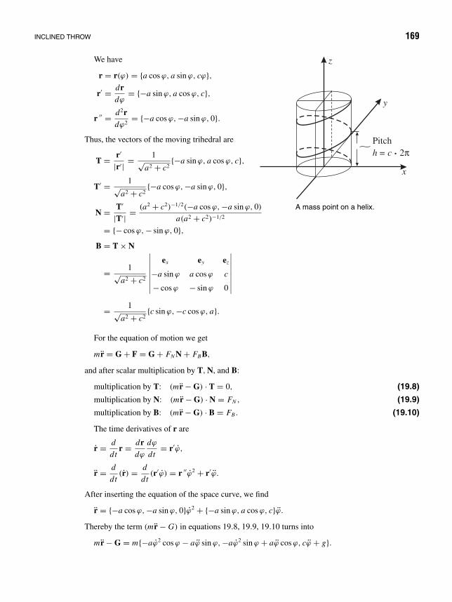
INCLINED THROW 169
y
z
x
Pitch= 2h c . π
A mass point on a helix.
We have
r = r(ϕ) = a cos ϕ, a sin ϕ, cϕ,r′ = dr
dϕ= −a sin ϕ, a cos ϕ, c,
r ′′ = d2rdϕ2
= −a cos ϕ, −a sin ϕ, 0.
Thus, the vectors of the moving trihedral are
T = r′
|r′| = 1√a2 + c2
−a sin ϕ, a cos ϕ, c,
T′ = 1√a2 + c2
−a cos ϕ, −a sin ϕ, 0,
N = T′
|T′| = (a2 + c2)−1/2(−a cos ϕ, −a sin ϕ, 0)
a(a2 + c2)−1/2
= − cos ϕ, − sin ϕ, 0,B = T × N
= 1√a2 + c2
∣∣∣∣∣∣∣∣ex ey ez
−a sin ϕ a cos ϕ c
− cos ϕ − sin ϕ 0
∣∣∣∣∣∣∣∣= 1√
a2 + c2c sin ϕ, −c cos ϕ, a.
For the equation of motion we get
mr = G + F = G + FN N + FBB,
and after scalar multiplication by T, N, and B:
multiplication by T: (mr − G) · T = 0, (19.8)
multiplication by N: (mr − G) · N = FN , (19.9)
multiplication by B: (mr − G) · B = FB . (19.10)
The time derivatives of r are
r = d
dtr = dr
dϕ
dϕ
dt= r′ϕ,
r = d
dt(r) = d
dt(r′ϕ) = r ′′ϕ2 + r′ϕ.
After inserting the equation of the space curve, we find
r = −a cos ϕ, −a sin ϕ, 0ϕ2 + −a sin ϕ, a cos ϕ, cϕ.
Thereby the term (mr − G) in equations 19.8, 19.9, 19.10 turns into
mr − G = m−aϕ2 cos ϕ − aϕ sin ϕ, −aϕ2 sin ϕ + aϕ cos ϕ, cϕ + g.

170 THE FREE FALL 19
After scalar multiplication by the vectors of the moving trihedral, it follows for equation
19.9: FN = (mr − G) · N = maϕ2, (19.11)
19.10: FB = (mr − G) · B = mga(a2 + c2
)−1/2, (19.12)
19.8: 0 = (mr − G) · T = m√a2 + c2
[(a2 + c2
)ϕ + cg
] ; (19.13)
thus
ϕ = −gc
a2 + c2; hence ϕ = C2 + C1t − g
2t2 c
a2 + c2.
From the initial conditions ϕ(t = 0) = ϕ0 and ϕ(t = 0) = 0, it follows for the two integrationconstants: C1 = 0 and C2 = ϕ0. Finally,
ϕ = ϕ(t) = ϕ0 − c
a2 + c2
g
2t2,
ϕ(t) = −cgt(a2 + c2
)−1.
For FN we get according to equation 19.11:
FN = mg2ac2t2
(a2 + c2)2,
and for the resulting guiding pressure
F =√
F2N + F2
B = mga(a2 + c2)−1/2 ·√
1 + g2c4
(a2 + c2)3t4 = F(t).
The path velocity is
v(t) = r = r′ϕ = |r′|ϕT = ϕ√
a2 + c2 · T.
The magnitude of the velocity—along the tangent—is
v(t) = ϕ√
a2 + c2 = −gtc√
a2 + c2.
The negative sign characterizes the “downward motion” (for c > 0) .(b) To determine ϕ(t) by means of the energy law, we compare the initial position z0(v(z0) = 0)
with an arbitrary intermediate position z. The result is
mgz0 = mgz + m
2v2
or, rewritten,
2g(z0 − z) = v2 = r 2 = r′2ϕ2 .
Using r′2 = a2 +c2 and z = cϕ with z0 = cϕ0, we obtain the following differential equation for ϕ(t):
ϕ2 + 2gc
a2 + c2(ϕ − ϕ0) = 0 ,

INCLINED THROW 171
or with the substitution ψ = ϕ − ϕ0:
ψ2 + 2gc
a2 + c2ψ = 0 or ψ = i
√2gc
a2 + c2· ψ = dψ
dt.
Separation of the variables leads to
i
√2gc
a2 + c2dt = dψ√
ψ,
and integration yields
i
√2gc
a2 + c2
∫dt =
∫dψ√
ψor i
√2gc
a2 + c2t = 2
√ψ,
and after forming the square:
ψ = − g
2t2 c
a2 + c2.
Resubstitution finally yields
ϕ = ψ + ϕ0 = ϕ(t) = ϕ0 − c
a2 + c2
g
2t2.
Problem 19.3: Spaceship orbits around the earth
A spaceship orbits around the earth at the height h above ground. Calculate (a) the orbital velocity,and (b) the orbital period such that zero gravity occurs in the spaceship. (c) Discuss these results forthe case h R.
Solution (a) Zero gravity ⇔ earth attraction = centrifugal force.
mv2
R + h= γ Mm
(R + h)2= gR2m
(R + h)2, because
γ Mm
R2= mg for h = 0
⇒ v = R
R + h
√(R + h)g “orbital velocity.”
(b)
v = path length
period= 2π(R + h)
T⇒ T = 2π
(R + h
R
)√R + h
g.
(c) For h R it follows that v ≈ √Rg and T ≈ 2π
√R/g.
The orbital velocity for R = 6371 km and g = 9.81m/s2 is then
v ≈ 7.9km
s,
and the orbital period T ≈ 84 min.

20 Friction
In general, any moving body undergoes a deceleration due to the interaction with itsenvironment being at rest. The occurring friction forces are always directed opposite to thedirection of motion; they are not conservative (the contour integral along a closed path isnonzero).
If we consider only the mechanical process, the energy conservation law does not apply:Kinetic energy is converted to heat.
Friction phenomena in a viscous medium
vFR( )vOil
Illustration of friction in a vis-cous medium.
The friction of a body in gases and liquids is governed bythe general ansatz
FR = −F(v)vv.
It always acts against the velocity v. The functionF(v) is in general not simple and must be determined empirically.
As an approximation two approaches prove successful.
Stokes’ friction FR = −βv, β = constant > 0 (holds, e.g., for rapidly moving missilesor for the motion in viscous liquids).
F II
F
T
Friction of a solid body on a support.
Newtonian friction FR = −γ vv, γ = constant > 0(holds, e.g., for slowly moving missiles).
Friction phenomena between solid bodies: A solidbody presses onto its support with the force F⊥. Onemay realize two distinct types of friction.
(a) Dynamic friction (v = 0)
The effective friction force is over a wide range independent of the area of support andthe velocity and is proportional to the force F⊥ pressing the body onto the area (supportload). Thus we may adopt the empirical ansatz:
FR = −µg F⊥ vv
(Coulomb),
where µg is called the dynamic friction coefficient.
172

FRICTION PHENOMENA IN A VISCOUS MEDIUM 173
(b) Static friction (v = 0)
If the body is at rest, tractive forces F acting parallel to the support area are just compen-sated by static friction. This applies as long as the acting force remains below a maximumvalue that is proportional to the support load. Only if F‖ becomes larger than a certain valueµh F⊥ does the body begin to move. It is vividly clear that this “limit force” is proportionalto the support load F⊥.
F
FII
F
T
The decomposition of the gravita-tional force in components normaland parallel to the inclination of theplane.
Thus, the body remains at rest as long as
F‖ < µh F⊥,
where µh is the static friction coefficient.Thus, static friction obeys a similar law as dynamic
friction does, although with another friction coeffi-cient.
Empirically, we obtain the relation for the coeffi-cients
0 < µg < µh .
Their magnitude depends sensitively on the surface properties.
Example 20.1: Free fall with friction according to Stokes
z
x
m
mgk
-β| |v k
k
k is the unit vector in the nega-tive z-direction, i.e., k = −ez .
As an example we consider the motion of a body (e.g., parachute)with the initial velocity v = v0 at the time t = 0. The motion isone-dimensional; the equation of motion reads
mz = −mg − β z,
or
mdv
dt= (−mg − βv). (20.1)
The gravitational force acts along the −z-direction; the frictionforce points opposite to the velocity.
After separation of the variables, we have
m dv
mg + βv= −dt,
m
v∫v0
dv
mg + βv= −
t∫0
dt = −t.
The integral to the left is solved by substituting mg + βv = u and dv = du/β:
m
v∫v0
dv
mg + βv= +m
β
mg+βv∫mg+βv0
du
u= m
βln
mg + βv
mg + βv0.
174 FRICTION 20
Therefore,
t = m
βln
(mg + v0β
mg + βv
).
Exponentiation of both sides of the equation yields
eβm t = mg + βv0
mg + βv;
and rewritten this reads
mg + βv0 = (mg + βv)eβm t .
Solving for v leads to
v(t) = −mg
β+(
mg
β+ v0
)e− β
m t . (20.2)
One easily sees from this velocity-time function that for increasing t the velocity v(t) approaches alimit value, that is, for large times v(t) becomes constant. Let us denote the limit velocity for largetimes by v∞. According to 20.2,
v∞ = limt→∞ v(t) = −mg
β. (20.3)
This may already be concluded from the dynamic equation 20.1 for the case of a vanishingacceleration z = 0. In 20.2 we will approximate the exponential function by the first two terms of thecorresponding Taylor expansion for small friction forces (β/m)t 1:
v(t) = −mg
β+(
v0 + mg
β
)(1 − βt
m+ · · ·
).
Investigation of the limit for β → 0 yields
limβ→0
v(t) = v0 − gt,
that is the expected result for the case without friction.We still determine z(t) and its limit for t → ∞: From 20.2 it follows by integration (dz/dt = v(t))
that
z(t) = −mgt
β− m
β
(v0 + mg
β
)e− β
m t + c2,
where, because z = 0 for t = 0, the integration constant is
c2 = m
β
(v0 + mg
β
)and therefore z(t) finally reads
z(t) = −mgt
β+ m
β
(v0 + mg
β
)(1 − e− β
m t)
,
limt→∞ z(t) = v∞t + m
β(v0 − v∞).

FRICTION PHENOMENA IN A VISCOUS MEDIUM 175
That means that for large times z increases linearly with the time. From z(t) one calculates theacceleration a(t) as
z(t) = a(t) = −β
m
(v0 + mg
β
)e− β
m t .
It vanishes for large times. Then the gravitational force and the friction force just balance each other.
Example 20.2: The inclined throw with friction according to Stokes
z
y
mg
α
v0
The inclined throw.
Adopted initial conditions: At the time t = 0, let
r(0) = 0,
v(0) = v0
= v0 cos α e2 + v0 sin α e3.
Equation of motion:
mr = −β r − mge3 or v + β
mv = −ge3.
To integrate this vectorial differential equation, we multiply by eβm t :
veβm t +
(β
m
)v e
βm t = −ge3e
βm t .
The left side of this equation is just the time derivative of v eβm t according to the product rule, so that
it may be integrated right now:
v eβm t = −
∫g e
βm t e3 dt = −g
m
βe
βm t e3 + c1.
Because v(0) = v0, c1 = v0 + g mβ
e3. Ordered by components, the velocity is
v = v0 cos α e− βm t e2 +
[−mg
β+(
v0 sin α + mg
β
)e− β
m t
]e3
or
v = −gm
β
(1 − e− β
m t)
e3 + v0e− βm t .
The position r(t) of the missile may be found by integration of the velocity:
r = −m
βv0 cos α e− β
m t e2 +[−mg
βt − m
β
(v0 sin α + mg
β
)e− β
m t
]e3 + c2
or
r = −gm
β
(t + m
βe− β
m t
)e3 − v0
m
βe− β
m t + c2 .

176 FRICTION 20
Because r(0) = 0, the integration constant is
c2 = m
βv0 cos α e2 + m
β
(v0 sin α + mg
β
)e3.
Inserting this integration constant, for the position we get
r = m
βv0 cos α
(1 − e− β
m t)
e2 +[−mg
βt + m
β
(v0 sin α + mg
β
)(1 − e− β
m t)]
e3.
Remark: The same results for r(t) and v(t) would have been found by separate considerations ofthe two differential equations
my + β y = 0,
mz + β z = −mg.
If one adopts the ansatz of Newtonian friction, the equation of motion of the problem is no longerseparable, because mr = −β|r|r − mge3 decays into
my + β√
y2 + z2 y = 0,
mz + β√
y2 + z2 z = −mg,
that is, in a set of coupled nonlinear differential equations. In most cases such equations may not besolved analytically. The linearity and nonlinearity of differential equations is discussed in Chapters 23and 25.
Discussion of the motion
For large times (t m/β) the exponential factor exp(− β
m t) tends to zero. That means(a) limt→∞ v(t) = −(mg/β)e3. The motion turns over to the vertical fall with constant limit
velocity. The horizontal velocity component vanishes for large times, namely, the motion in y-direction comes to rest.
(b) limt→∞ y(t) = (m/β)v0 cos α ≡ y0. With increasing time the motion in the horizontal directiontends asymptotically against the maximum distance y0.
The path equation may be found explicitly by eliminating the time parameter from the equationsfor r · e2 and r · e3. We get
z(y) = m2
β2g ln
(1 − βy
mv0 cos α
)+(
v0 sin α + mg
β
)y
v0 cos α.
To investigate the trend of the trajectory for very low friction, we may employ the Taylor expansionof the logarithm:
ln(1 + x) = x − x2
2+ x3
3− + · · · .
Then
z(y) = −m2
β2g
[βy
mv0 cos α+ 1
2
(βy
mv0 cos α
)2]
+(
v0 sin α + mg
β
)y
v0 cos α+ · · ·

MOTION IN A VISCOUS MEDIUM WITH NEWTONIAN FRICTION 177
= − g
2v20 cos2 α
y2 + y tan α + R.
Here
R = −1
3
β
mg
(y
v0 cos α
)3
− · · ·
is a remainder term. Note that the first two terms are the same as in the formula of the parabola ofinclined throw, equation (19.7).
From this relation we may realize that
(a) For vanishing friction the result approaches the throw parabola.
(b) If friction is present, the trajectory runs below the throw parabola; for small y, it osculates theparabola (osculation of second order).
z
y
10β0
l10β0l3β0
l2β0lβ0
3β0 2β0 β0 β=0
Trajectories for the inclined throw with different friction.
Motion in a viscous medium with Newtonian friction
We consider the motion of a body affected only by a velocity-dependent friction force. Thecase of Stokes friction has already been treated in the preceding example. We thereforenow consider Newtonian friction.
Let the (necessarily rectilinear) motion proceed along the x-direction; the unit vector e1
is therefore omitted. We choose the initial conditions v(t = 0) = v0, x(t = 0) = 0.

178 FRICTION 20
The equation of motion reads
mx = −γ x2,
and the separation of variables yields
mdv
v2= −γ dt.
The integration leads to
−m1
v= −γ t + c1.
From the initial conditions it follows that
c1 = − m
v0.
By inserting the integration constant and solving for v, we get the velocity
v(t) = m
γ v0t + mv0.
The position is obtained by a further integration. To solve the integral we substitute z =γ v0t + m, dz = γ v0dt .
x = mv0
∫dt
γ v0t + m= m
γ
∫dz
z= m
γln(γ v0t + m) + c2.
The integration constant is c2 = −(m/γ ) ln m. Hence, the path is
x(t) = m
γln( γ
mv0t + 1
).
Discussion: For increasing time t → ∞, we have the two limits
limt→∞ v(t) = 0 , lim
t→∞ x(t) = ∞.
FR=0
Newton ~F vR2
Stokes ~F vR
x
tIllustration of the path x(t) for different cases of friction.

GENERALIZED ANSATZ FOR FRICTION: 179
Although the velocity becomes smaller and smaller, the body moves arbitrarily far underthe influence of Newtonian friction.
Generalized ansatz for friction:
In the following we adopt a more general ansatz for the velocity-dependent friction force,which is of particular interest for low velocities, namely
FR = −vn vv.
Here n ≥ 0 because the friction shall decrease when v decreases. The equation of motionthen reads
mx = −x n
ordv
vn= −
mdt for n = 1
(n = 1 corresponds to Stokes friction). Integration yields
v−n+1
−n + 1= −
mt + C1, C1 = v1−n
0
1 − n,
with v(t = 0) = v0. From there it follows for the velocity that
v(t) =(v1−n
0 − (1 − n)
mt)1/(1−n)
.
Here one may distinguish two cases:
• 0 ≤ n < 1:The expression in the brackets may vanish. Therefore, the body comes to rest after somefinite time t0;
t0 = m
v1−n0
1 − n.
As soon as t ≥ t0, the derived formula no longer holds; the body remains at rest.
• n > 1:The body does not come to rest completely, but its velocity becomes arbitrarily smallbecause
limt→∞ v(t) = lim
t→∞1
(v−α0 + α
m t)1/α= 0 with α = n − 1 > 0.

180 FRICTION 20
The necessary second integration becomes simpler by considering v(x(t)). Accordingto the chain rule,
dv
dt= dv
dx· dx
dt= dv
dxv.
Insertion into the equation of motion yields
dv · v1−n = −
mdx .
Integration yields
1
2 − nv2−n = −
mx + C2.
With
v(x = 0) = v(t = 0) = v0,
we get
C2 = 1
2 − nv2−n
0 .
Hence
x(v) = m
1
n − 2(v2−n − v2−n
0 ).
Or, by inserting v(t), the path is obtained as a function of the time as
x(t) = m
1
n − 2
[(v1−n
0 − (1 − n)
mt) n−2
n−1 − v2−n0
].
Here two distinct cases also exist, which may most simply be extracted from the functionx(v), namely
0 ≤ n < 2: limv→0
x(v) = m
1
2 − nv2−n
0 = l,
n > 2: limv→0
x(v) = m
βlimv→0
(1
vβ− 1
vβ
0
)= ∞
(with β = n − 2 > 0—for n = 2; see Newtonian friction).In total, we thus may distinguish between three types of motion, namely
(a) 0 ≤ n < 1:The motion comes to rest at the time t0 at the distance l.
(b) 1 ≤ n < 2:The velocity tends to zero while the body approaches a finite limit point at the distance l.

GENERALIZED ANSATZ FOR FRICTION: 181
(c) n ≥ 2:The velocity asymptotically approaches zero while the distance increases beyond anylimit.
FR
n=1
1< <2nn>2
n<1
vDifferent types of friction.
The already treated cases are limit cases of thetypes of motion (b) (Stokes, n = 1) and (c) (New-ton, n = 2). The figure illustrates the distincttrends. For very low velocities the friction force—independent of the coefficient—tends to zero thefaster the larger the exponent n is. On the otherhand, for small n the deceleration decreases soslowly (i.e., the decelerating force is for small nso strong) that the motion even comes to rest.
Problem 20.3: Free fall with Newtonian friction
A body begins to fall at the time t = 0 at the point z = 0 with the initial velocity v0. Determinethe fall velocity v(t) and the path z(t), assuming Newtonian friction. Which approximations hold forsmall times if v0 = 0?
Solution The equation of motion reads
mz = −mg − γ z|z| or v = −g
(1 + γ
mgv|v|
)= −g
(1 + v|v|
v2∞
).
With the abbreviation
v∞ =√
mg
γfollows v2
∞
v∫v0
dv
v2∞ + v|v| = −g
t∫0
dt.
Integration of the equation of motion yields
−gt =
⎧⎪⎪⎪⎪⎪⎪⎪⎪⎪⎨⎪⎪⎪⎪⎪⎪⎪⎪⎪⎩
[v∞ arctan
v
v∞
]v
v0
for v ≥ 0,
[v∞ Artanh
v
v∞
]v
v0
for −v∞ < v < 0,
[v∞ Arcoth
v
v∞
]v
v0
for v < −v∞.
One therefore has to distinguish three cases, depending on the magnitude of the initial velocity.1. v0 ≥ 0. Initial velocity and gravitational force are opposite to each other. After integration it
follows that
−gt = v∞ arctanv
v∞− v∞ arctan
v0
v∞.

182 FRICTION 20
The meaning of the constant term becomes obvious if v = 0:
gt0 = gt (v = 0) = v∞ arctanv0
v∞,
and thus
−g(t − t0) = v∞ arctanv
v∞or
v = −v∞ tang
v∞(t − t0).
Because the motion must be continuous also for t = t0, the integration between t0 and t yields
−g(t − t0) = v∞ Artanhv
v∞− 0,
hence
v = −v∞ tanhg
v∞(t − t0); t ≥ t0.
The body moves upward against the gravitational force, comes to rest at t0, and falls downward.2. −v∞ < v0 ≤ 0. Integration yields
−gt = v∞ Artanhv
v∞− v∞ Artanh
v0
v∞.
If we imagine the velocity function as continued for negative times t < 0, the constant term againhas a clear meaning:
t0 = t (v = 0) = v∞g
Artanhv0
v∞.
The velocity function may then be expressed by
v = −v∞ tanhg
v∞(t − t0).
3. v0 < −v∞.
−gt = v∞ Arcothv
v∞− v∞ Arcoth
v0
v∞.
Similar to the other cases we abbreviate
t (v = −∞) = t− = v∞g
Arcothv0
v∞
and thus
v = −v∞ cothg
v∞(t − t−).
In all three cases the velocity asymptotically approaches the limit velocity
−v∞ = −√
mg
γ.

GENERALIZED ANSATZ FOR FRICTION: 183
v v v
t0 t0 t0
v0>0 < <0v0 v0<
–v
–v –v
t t t8
8 8
Velocity as function of time for three different initial velocities.
The function z(t) may be calculated straightforward from v(t).1.
z = v∞∫
tang
v∞(t0 − t) dt = +m
γln cos
g
v∞(t0 − t) + K1, t ≤ t0;
z = −v∞∫
tanhg
v∞(t − t0) dt = −m
γln cosh
g
v∞(t − t0) + K1, t ≥ t0;
where
K1 = −m
γln cos
g
v∞t0.
2.
z = −m
γln cosh
g
v∞(t − t0) + K2 ,
K2 = m
γln cosh
(− g
v∞t0
).
3.
z = −v∞∫
cothg
v∞(t − t−) dt = −m
γln sinh
g
v∞(t − t−) + K3 ,
K3 = m
γln sinh
(− gt−
v∞
).
In particular, for v0 = 0 one has t0 = 0, and therefore
v = −v∞ tanhgt
v∞,
z = −v2∞g
ln coshgt
v∞.
There hold the series expansions
sinh u = u + u3
3!+ · · · ,

184 FRICTION 20
cosh u = 1 + u2
2!+ u4
4!+ · · · ,
ln(1 + u) = u − u2
2+ − · · · .
For small times (t v∞/g) we may then write approximately1. Velocity:
v ≈ −u + 16 u3
1 + 12 u2
v∞ ≈ −v∞u
(1 − 1
3u2
)with u = gt
v∞,
≈ −gt
(1 − 1
3
(gt
v∞
)2)
.
2. Path:
z ≈ −v2∞g
ln
(1 + u2
2+ u4
24
)≈ −v2
∞g
[u2
2+ u4
24− 1
2
(u4
4+ · · ·
)],
≈ −1
2gt2
(1 − 1
6
(gt
v∞
)2)
.
Problem 20.4: Motion of an engine with friction
An engine of mass m moves without driving force but under the influence of the friction forcef (v) = α + βv2 on horizontal rails. Let the initial velocity be v0.
(a) After which time does the engine come to rest? What is the maximum deceleration time(v0 → ∞)?
(b) What distance has then been covered?
Solution The equation of motion reads
mx = − f (v) = −α − β x2
and will be integrated after separation of the variables:(a)
mdv
dt= −(α + βv2);
m
β
0∫v=v0
dv
α/β + v2= −
t0∫t=0
dt;
m
β
√β
α
(arctan 0 − arctan
√β
αv0
)= −t0;

GENERALIZED ANSATZ FOR FRICTION: 185
t0 = m√αβ
arctan
√β
αv0; lim
v0→∞ t0 = m√αβ
π
2.
(b) If we use x and v as variables, the equation of motion reads
mdv
dx
dx
dt= −(α + βv2).
This is transformed and integrated:
m
2β
0∫v=v0
2βv
α + βv2dv = −
x0∫x=0
dx;
m
2β
[ln α − ln
(α + βv2
0
)] = −x0.
The total path covered is therefore
x0 = m
2βln
(1 + β
αv2
0
).
For an infinite initial velocity v0 the engine covers an infinite distance until the rest, although thedeceleration to velocity 0 takes only the finite time (m/
√αβ)(π/2).
Example 20.5: The inclined plane
So far we have considered the motion of a free massive body under the action of external forces. If itsfreedom of motion is, however, restricted to a defined area or line by certain constraints, one speaks ofa bound motion. A constraining force must then act on the body that keeps it on the prescribed path.
In a motion on a solid area or rail the body undergoes a reactive force by the support that justbalances the normal component of the force acting on it. When taking into account this constrainingforce, the equation of motion may be formulated according to the second Newtonian axiom.
α
e
f FR
Fs
Fs FsII
T
Forces acting on a mass at theinclined plane
The simplest example is the motion on the inclined plane.
(a) Without friction
We introduce the following denotations (compare figure):Fs : gravitational force;F‖
s , F⊥s : parallel and normal components of the weight force;
FR : reactive force;s: covered path.The following relations exist between the forces:
F⊥s = −FR
(according to the third Newtonian axiom);
Fs = F⊥s + F‖
s = −mge3;F‖
s = mg sin α e (see figure).

186 FRICTION 20
The equation of motion is then
mse =∑
i
Fi = Fs + FR = F‖s = mg sin α e.
Only the parallel component of the weight force causes the acceleration (slope drift):
s = g sin α ≡ g′.
This is exactly the differential equation of the free fall with an earth acceleration reduced by the factor
α
e
e3
FR
Fs
Fs
T FsII
s
Decomposition of the forces on the in-clined plane.
sin α. Twofold integration leads again to the solutions
v(t) = g sin αt + v0,
s(t) = 1
2g sin αt2 + v0t + s0.
(b) With friction
Besides the constraining force FR along the area normal,there also acts a parallel component f on the body thatalways points opposite to the friction force. According tothe figure, the support force is
F⊥s = cos α mg,
and therefore the dynamic friction force is
f = ∓µgmg cos α e if v>< 0.
Hence, the equation of motion reads
ms e = Fs + FR + f = F‖s + f = mg(sin α ∓ µg cos α)e
if v>< 0.
This again yields the differential equation
s = g(sin α ∓ µg cos α) ≡ g‖,
with the solutions
v(t) = g(sin α ∓ µg cos α)t + v0, for v>< 0,
s(t) = 1
2g(sin α ∓ µg cos α)t2 + v0t + s0 .
If the motion points downward (v > 0), we may distinguish among three distinct cases:
(a) g‖ > 0: that is, tan α > µg or α > αg = arctan µg . The body is positively accelerated.
(b) g‖ = 0: tan α = µg , α = αg . The body moves uniformly, the gravitational force component andthe friction mutually cancel.
(c) g‖ < 0: tan α < µg . The body is decelerated and comes to rest after the time
t = v0
g(µg cos α − sin α).

GENERALIZED ANSATZ FOR FRICTION: 187
If v < 0, namely the direction of motion is upward, then g‖ = g(sin α + µg cos α) > 0; the bodycomes to rest in any case. It depends on the magnitude of the coefficient µg of the now-acting staticfriction whether the body begins to move out of the state of rest.
The inclined plane allows us to determine the two friction coefficients by varying the slope angle α:
µg = tan α if the body uniformly moves (v > 0),
µh = tan α if the body just starts sliding.
Problem 20.6: Two masses on inclined planes
α
α
β
β
e1
m1
m1g m2g
e2
m2F1 F2
A
TT
Two masses on inclined planes.
Two masses m1 and m2 are lying each on oneof two joined planes that enclose the anglesα and β with the horizontal (see figure). Thetwo masses are connected by a massless andnonductile rope running over a roller fixed atpoint A.
Determine the acceleration a of the massesm1 and m2, taking the friction into account.
Solution The friction mentioned in the problem is dy-
namic(
FR = −µg F⊥v /v)
. Because the ve-
locity v points along e1 or e2, respectively, thequantity v /v just equals e1 or e2!
Hence
m1ae1 = m1g sin α e1 − T e1 − µg F⊥1 e1 (20.4)
and−m2ae2 = m2g sin β e2 − T e2 + µg F⊥
2 e2. (20.5)
T is the string tension. The signs in front of the two last terms on the right-hand side (the frictionterms) are valid only for positive acceleration, a > 0. We have to check this at the end of thecalculation. We now have to calculate F⊥
1 and F⊥2 . From the sketch we see that
F⊥1 = m1g cos α and F⊥
2 = m2g cos β .
F⊥1 and F⊥
2 inserted in 20.4 and 20.5 yield
m1ae1 = m1g sin α e1 − T e1 − µgm1g cos α e1, (20.6)
−m2ae2 = m2g sin β e2 − T e2 + µgm2g cos β e2. (20.7)
From 20.6 it follows that T = m1g sin α − m1a − µgm1g cos α. T is now inserted in 20.7:
−a(m1 + m2) = m2g sin β − m1g sin α + µgm1g cos α + µgm2g cos β
⇔ a = m1 sin α − m2 sin β − µgm1 cos α − µgm2 cos β
m1 + m2g.
Thus, the acceleration has been determined. Finally, we consider two special cases:(1) µg = 0, that is, there is no friction; therefore,
a = m1 sin α − m2 sin β
m1 + m2g .

188 FRICTION 20
(2) α = β = 90; the acceleration then becomes
a = m1 − m2
m1 + m2g.
Problem 20.7: A chain slides down from a table
e Z
A chain sliding down from a table
A uniform chain of total length a hangs with a piece of lengthb (0 ≤ b ≤ a) over the edge of a plane table. Calculate thetime in which the chain slides from the table under the influenceof gravity but without friction. Let the initial velocity be 0 (seefigure).
Investigate the same problem, assuming now a dynamic fric-tion µg .
Solution (a) Without frictionThe length of the fraction of the chain hanging vertically down is denoted by z; the mass per unit
length is . The equation of motion then reads
az = zg ⇔ d2z
dt2= g
az. (20.8)
This differential equation states that z(t) differentiated twice with respect to t reproduces itself upto the factor g/a. This condition is fulfilled by one of the two independent exponential functions
e√
g/a t and e−√
g/a t
such that the general solution reads
z(t) = Ae√
g/a t + Be−√
g/a t . (20.9)
A and B are integration constants, which are determined from the initial conditions
z(0) = b = A + B,
z(0) = 0 = A
√g
a− B
√g
a⇒ A − B = 0 . (20.10)
This yields A = b/2, B = b/2, and therefore for 20.9
z(t) = b
2
(e√
g/a t + e−√
g/a t)
= b cosh
√g
at. (20.11)
The time T of sliding follows from the condition
z(T ) = a = b
2
(e√
g/aT + e−√
g/aT)
. (20.12)
From there it follows with x = e√
g/aT that
2a
b= x + 1
x⇔ x2 − 2a
bx = −1
⇒ x1,2 = a
b±√
−1 + a2
b2= a
b± 1
b
√a2 − b2 = 1
b(a ±
√a2 − b2) . (20.13)
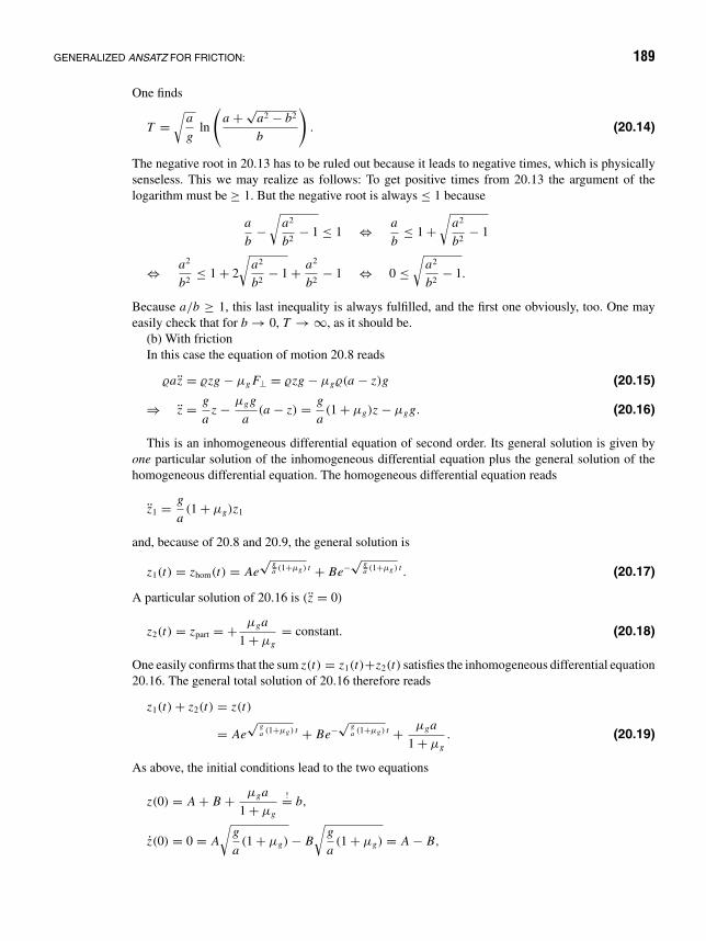
GENERALIZED ANSATZ FOR FRICTION: 189
One finds
T =√
a
gln
(a + √
a2 − b2
b
). (20.14)
The negative root in 20.13 has to be ruled out because it leads to negative times, which is physicallysenseless. This we may realize as follows: To get positive times from 20.13 the argument of thelogarithm must be ≥ 1. But the negative root is always ≤ 1 because
a
b−√
a2
b2− 1 ≤ 1 ⇔ a
b≤ 1 +
√a2
b2− 1
⇔ a2
b2≤ 1 + 2
√a2
b2− 1 + a2
b2− 1 ⇔ 0 ≤
√a2
b2− 1.
Because a/b ≥ 1, this last inequality is always fulfilled, and the first one obviously, too. One mayeasily check that for b → 0, T → ∞, as it should be.
(b) With frictionIn this case the equation of motion 20.8 reads
az = zg − µg F⊥ = zg − µg(a − z)g (20.15)
⇒ z = g
az − µgg
a(a − z) = g
a(1 + µg)z − µgg. (20.16)
This is an inhomogeneous differential equation of second order. Its general solution is given byone particular solution of the inhomogeneous differential equation plus the general solution of thehomogeneous differential equation. The homogeneous differential equation reads
z1 = g
a(1 + µg)z1
and, because of 20.8 and 20.9, the general solution is
z1(t) = zhom(t) = Ae√
ga (1+µg ) t + Be−
√ga (1+µg ) t . (20.17)
A particular solution of 20.16 is (z = 0)
z2(t) = zpart = + µga
1 + µg= constant. (20.18)
One easily confirms that the sum z(t) = z1(t)+z2(t) satisfies the inhomogeneous differential equation20.16. The general total solution of 20.16 therefore reads
z1(t) + z2(t) = z(t)
= Ae√
ga (1+µg ) t + Be−
√ga (1+µg ) t + µga
1 + µg. (20.19)
As above, the initial conditions lead to the two equations
z(0) = A + B + µga
1 + µg
!= b,
z(0) = 0 = A
√g
a(1 + µg) − B
√g
a(1 + µg) = A − B,

190 FRICTION 20
with the solution
A = b
2− µga
2(1 + µg), B = b
2− 1
2
µga
(1 + µg).
Thus, the complete solution reads
z(t) =(
b
2− µga
2(1 + µg)
)[e√
ga (1+µg ) t + e−
√ga (1+µg ) t
]+ µga
1 + µg. (20.20)
The time of sliding T is determined by the equation
z(T ) = a =(
b
2− µga
2(1 + µg)
)[e√
ga (1+µg ) T + e−
√ga (1+µg ) T
]+ µga
1 + µg
⇒ a
(1
1 + µg
)=(
b − µg
1+µga)
2
(x + 1
x
), (20.21)
where
x = e√
ga (1+µg ) T . (20.22)
The quadratic equation 20.21 has the solution
x1,2 =a(
11+µg
)b(
1 − µg
1+µg
ab
) ± 1
b(
1 − µg
1+µg
ab
)√
a2
(1
1 + µg
)2
− b2
(1 − µg
1 + µg
a
b
)2
.
The solution x2 drops out similarly as above. Therefore, the time of sliding T is evaluated as
T =√
a
g(1 + µg)× ln
a +√
a2 − (b + µg(b − a)
)2
b + µg(b − a). (20.23)
We note that it may be seen from equation 20.16 that the chain begins to slide only then if z > 0,that is,
b >µg
1 + µga.
The time of sliding T increases under friction. This is not seen from 20.23 at first glance, and oneneeds to perform an expansion by µg , which will be saved here.
Problem 20.8: A disk on ice—the friction coefficient
ez
ex mg
FR
z
x
N
Forces acting on a sliding disk.
A disk is sliding on ice. At a certain point of the straightpath it has the velocity v0. It comes to rest at the distancex0 beyond this point. Determine the friction coefficient(e.g., for v0 = 40 km/h; x0 = 30 m).
Solution The initial conditions are
t = 0, x = 0, v = v0,
t = t0, x = x0, v = 0.

GENERALIZED ANSATZ FOR FRICTION: 191
The individual forces are denoted as follows:
W = −mgez (weight),
N = −W (normal force),
FR = −µg|N| ex ⇒FR = −µgmgex (friction force).
For the equation of motion one then obtains
mdvdt
ex = −µgmgex ⇒ dv
dt= −µgg.
Separation of the variables and integration yield
v∫v0
dv′ = −µgg
t∫0
dt ′ ⇒ v = v0 − µggt
andx∫
0
dx ′ =t∫
0
(v0 − µggt ′) dt ′ ⇒ x = v0t − 1
2µggt2.
The disk comes to rest if v = 0, namely at the time t0 = v0/µgg ⇒ inserted in x : x0 =(1/2)(v2
0/µgg), or solved for the friction coefficient: µg = (1/2)(v20/x0g) ≈ 0.21.
Problem 20.9: A car accident
An accident happens on a straight-plane village street (allowed velocity 50 km/h). After activatingthe brakes, the car slides 39 m until it stops (friction coefficient: µ = 0.5).
mg
FR
z
x
R
Forces acting on a sliding car.
Find out whether the driver is guilty.
Solution Because the weight mg and the reactive force mutually cancel eachother, only the friction force FR acts on the car. The equation ofmotion then reads
md2x
dt2= −µmg ⇒ d2x
dt2= −µg.
We now have
d2x
dt2= d
dt
(dx
dt
)= dx
dx
dx
dt= v
dv
dx
⇒ vdv
dx= −µg
⇒0∫
v0
v dv = −µg
x0+s∫x0
dx,

192 FRICTION 20
where x0 is the position where full breaking begins, and s is the braking distance. Thus we get
1
2v2
0 = µgs ⇒ v0 = √2µgs.
With the numerical data it follows that
v20 = 2 · 0.5 · 9.81 · 39
m2
s2
⇒ v0 = 19.56m
sor v0 = 70.42
km
h.
The driver drove too fast by about 20 km/h.
Problem 20.10: A particle on a sphere
Let a particle of mass m be positioned at the “north pole” of a frictionless smooth sphere of radiusb. After a small displacement let it slide down at the sphere. At which time does it separate from thesphere, and what is its velocity in that moment?
Solution If the particle is at P , it is pressed to the sphere by the normal force
N = −mg sin θ er ,
while the centrifugal force
Z = (mv2)/b er
tries to pull it off the sphere. At the moment at which both forces are balancing each other,
N + Z = 0,
the particle separates from the sphere!
et
ere2
e1
N
h
x
ym
b
Z
PW
θ
s
Forces acting on a particle on a sphere.
(a) Solution via the energy law: One has12 mv2 + mgh = T + V = E = mgb, where Eremains constant in time. Then
v2 = 2g(b − h) = 2gb(1 − sin θ)
and, therefore,
N + Z = −mg sin θ er + mv2
ber
= [2mg(1 − sin θ) − mg sin θ ] er .
In order to have N+Z = 0, it must hold that
2mg(1 − sin θ) − mg sin θ = 0
or
3 sin θ = 2, i.e., sin θ = 2
3,
θ = 41.8.

GENERALIZED ANSATZ FOR FRICTION: 193
From there we immediately find that at the moment of separation
h = 2
3b and v =
√2
3gb .
(b) Solution via the equation of motion: Consider the sphere as (locally) an inclined plane. At Pthere acts the slope drift
H = −mg cos θ et .
We call s the distance of the particle from the north pole, as measured along the surface of the sphere.Because
s = b(π
2− θ
),
we have
s = −bθ .
Hence, the equation of motion reads
−md2s
dt2et − H = −m
d2s
dt2et + mg cos θet = 0
or
−d2s
dt2+ g cos θ = bθ + g cos θ = 0.
Multiplication by θ yields
bθ θ + g cos θ θ = 0.
Integration of this differential equation leads to
1
2bθ 2 + g sin θ = c.
For t = 0, we have θ = 0 and θ = 90; thus c = g
⇒ θ2 = −2g
b(sin θ − 1).
For the moment of separation, we obtain
N + Z = m
(v2
b− g sin θ
)er = 0
or with v = bθ :
θ 2b − g sin θ = −2g(sin θ − 1) − g sin θ = 0
⇒ 3 sin θ = 2 or sin θ = 2
3; θ ≈ 41 49′.
For the velocity results,
v = θb = √2g(1 − sin θ)b =
√2
3gb.

194 FRICTION 20
Problem 20.11: A ladder leans at a wall
x
yz
lco
sθ
l sin θ
( sin )l θ2
-
θ
B
NW
NF
Ff
C
A
F gg=m
Forces acting on the ladder.
A ladder of length l and mass m leans at a vertical wall,enclosing the angle θ with the wall. The gravity force op-erates on the center of the ladder (see figure). The frictioncoefficient between the ground and ladder is µh , while thefriction between the wall and ladder is being neglected.
Determine the maximum angle θ at which the laddermay lean against the wall without sliding down.
Solution The forces acting on the ladder are the reactive force NF ez
at point A and the reactive force NW ex at point B.In addition, at A the friction force −Ff ex still acts in
the negative x-direction. The gravitational force −Fgez =−mgez acts on the center of the ladder.
The conditions that the system is in equilibrium are
(a) The sum over all forces must be zero.
(b) The sum over all torques with respect to a point mustbe zero.
From the figure we find the component representation:∑i
F xi = 0 : Nw − Ff = 0, (20.24)∑
i
F zi = 0 : −mg + NF = 0. (20.25)
The torques acting with respect to point A are caused by the forces −Fgez = −mgez and Nwex .We obtain
MA =∑
i
ri × Fi =(
−mg
(l
2sin θ
)+ Nw(l cos θ)
)ey = 0, (20.26)
or resolved for Nw:
Nw = mg
2tan θ. (20.27)
According to equation 20.24, the friction force Ff is
Ff = mg
2tan θ. (20.28)
Because the friction force cannot exceed the product of reactive force NF and friction coefficient µh
(see figure),
Ff (max) = NFµh = mgµh, (20.29)
we obtain as equilibrium condition
Nw = mg
2tan θ = Ff < Ff (max) = mgµh , (20.30)

GENERALIZED ANSATZ FOR FRICTION: 195
or
mg
2tan θ < mgµh ,
and for the angle θ :
tan θ < 2µh . (20.31)
The maximum angle θ is independent of the mass and length of the ladder. It is only a function of thefriction coefficient µh .
Problem 20.12: A mass slides under static and dynamic friction
m1
e1
e2
m3
m2
A sliding mass.
Two masses of m1 = 6 kg and m2 = 10 kg are fixed to anonstretchable rope that runs over a roller (see figure). The staticfriction coefficient for m1 and the support has the value µh =0.625. The dynamic friction coefficient is µg = 0.33.
(a) What is the minimum value of the mass m3 such that m1 doesnot move?
(b) What is the acceleration of the system if the mass m3 isremoved?
Solution (a) If the system is at rest, a static friction force FH acts on therope that is caused by the masses m1 and m3 and the support area:
FH = −µH F⊥ · v1
v1.
v1 points, however, along −e1; hence FH = µH (m1 + m3)ge1. The forces acting along −e1 are
−(m1 + m3)ae1 = −T e1 + µH (m1 + m3)ge1, (20.32)
and the forces acting along e2 are
m2ae2 = −T e2 + m2ge2, (20.33)
where T is the rope tension. Insertion of T from 20.33 in 20.32 yields
a = m2g − µH (m1 + m3)g
m1 + m2 + m3. (20.34)
We get as equilibrium condition
m3 = m2
µH− m1, m3 = 10 kg.
(b) If the system moves, µH must be replaced by µG (m3 = 0):
a = gm2 − µG m1
m1 + m2; a = 0.5 g.

21 The HarmonicOscillator
The eminent meaning of the harmonic oscillator is due to the fact that it does not occur inmechanics only, but in an analogous manner governs extended sections of electrodynamicsand atomic physics. Many complicated vibrational processes may be approximately de-scribed as harmonic oscillations and thus be treated simply in this way. The reason is thefollowing: In the equilibrium (at x = 0) the forces acting on the mass point must vanish,that is, F = −∇V = 0. If one expands the potential in a Taylor series
V (x) = V0 + a1x + a2
2x2 + . . . ,
the equilibrium condition implies that a1 = 0 must hold, just because F(0) = 0. Therefore,
V (x) = V0 + a2
2x2 + . . .
must hold. For small displacements from the equilibrium the potential is therefore alwaysharmonic. In mechanics we are dealing with a harmonic oscillator if a force acting on abody is proportional to, but oppositely directed to, its displacement from the rest position.This linear force law may be generated by a spring obeying Hooke’s law (see also p. 162in Section 18). To simplify the problem, we consider the harmonic oscillator only in thex-direction, i.e., the force law is
F = −kxe1.
For the linear force law, obviously
curl F = −e2∂
∂z(kx) + e3
∂
∂y(kx) = 0.
This implies: The force is conservative. Consequently, the energy law also holds:
1
2mv2 + V (x) = E = constant.
196
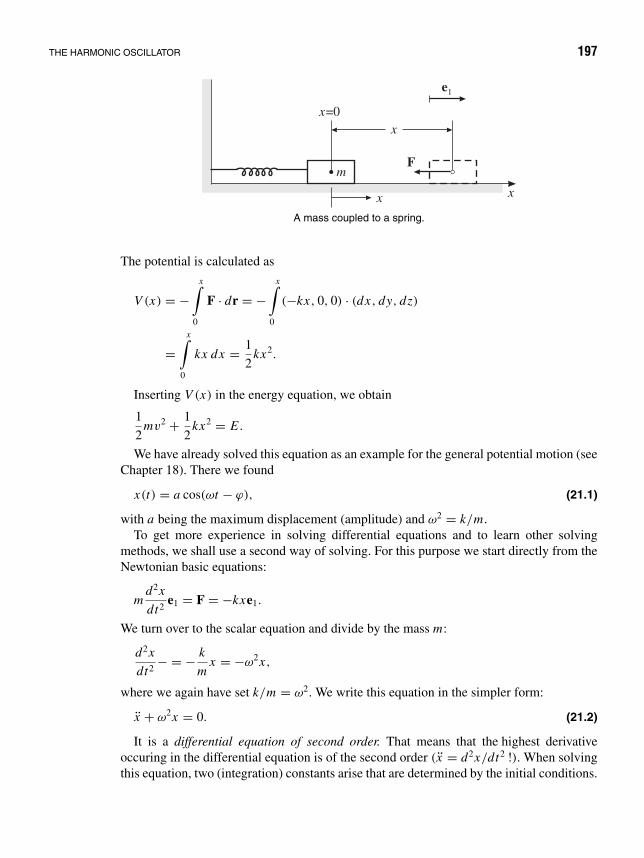
THE HARMONIC OSCILLATOR 197
x=0
xx
x
F
e1
m
A mass coupled to a spring.
The potential is calculated as
V (x) = −x∫
0
F · dr = −x∫
0
(−kx, 0, 0) · (dx, dy, dz)
=x∫
0
kx dx = 1
2kx2.
Inserting V (x) in the energy equation, we obtain
1
2mv2 + 1
2kx2 = E .
We have already solved this equation as an example for the general potential motion (seeChapter 18). There we found
x(t) = a cos(ωt − ϕ), (21.1)
with a being the maximum displacement (amplitude) and ω2 = k/m.To get more experience in solving differential equations and to learn other solving
methods, we shall use a second way of solving. For this purpose we start directly from theNewtonian basic equations:
md2x
dt2e1 = F = −kxe1.
We turn over to the scalar equation and divide by the mass m:
d2x
dt2− = − k
mx = −ω2x,
where we again have set k/m = ω2. We write this equation in the simpler form:
x + ω2x = 0. (21.2)
It is a differential equation of second order. That means that the highest derivativeoccuring in the differential equation is of the second order (x = d2x/dt2 !). When solvingthis equation, two (integration) constants arise that are determined by the initial conditions.
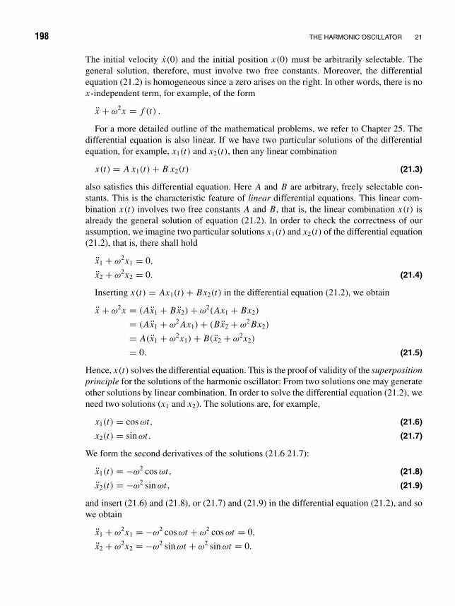
198 THE HARMONIC OSCILLATOR 21
The initial velocity x(0) and the initial position x(0) must be arbitrarily selectable. Thegeneral solution, therefore, must involve two free constants. Moreover, the differentialequation (21.2) is homogeneous since a zero arises on the right. In other words, there is nox-independent term, for example, of the form
x + ω2x = f (t) .
For a more detailed outline of the mathematical problems, we refer to Chapter 25. Thedifferential equation is also linear. If we have two particular solutions of the differentialequation, for example, x1(t) and x2(t), then any linear combination
x(t) = A x1(t) + B x2(t) (21.3)
also satisfies this differential equation. Here A and B are arbitrary, freely selectable con-stants. This is the characteristic feature of linear differential equations. This linear com-bination x(t) involves two free constants A and B, that is, the linear combination x(t) isalready the general solution of equation (21.2). In order to check the correctness of ourassumption, we imagine two particular solutions x1(t) and x2(t) of the differential equation(21.2), that is, there shall hold
x1 + ω2x1 = 0,
x2 + ω2x2 = 0. (21.4)
Inserting x(t) = Ax1(t) + Bx2(t) in the differential equation (21.2), we obtain
x + ω2x = (Ax1 + Bx2) + ω2(Ax1 + Bx2)
= (Ax1 + ω2 Ax1) + (Bx2 + ω2 Bx2)
= A(x1 + ω2x1) + B(x2 + ω2x2)
= 0. (21.5)
Hence, x(t) solves the differential equation. This is the proof of validity of the superpositionprinciple for the solutions of the harmonic oscillator: From two solutions one may generateother solutions by linear combination. In order to solve the differential equation (21.2), weneed two solutions (x1 and x2). The solutions are, for example,
x1(t) = cos ωt, (21.6)
x2(t) = sin ωt. (21.7)
We form the second derivatives of the solutions (21.6 21.7):
x1(t) = −ω2 cos ωt, (21.8)
x2(t) = −ω2 sin ωt, (21.9)
and insert (21.6) and (21.8), or (21.7) and (21.9) in the differential equation (21.2), and sowe obtain
x1 + ω2x1 = −ω2 cos ωt + ω2 cos ωt = 0,
x2 + ω2x2 = −ω2 sin ωt + ω2 sin ωt = 0.

THE HARMONIC OSCILLATOR 199
Both approaches fulfill our differential equation. Moreover, sine and cosine are linearlyindependent functions, that is, there is no constant C such that C sin ωt = cos ωt holds forall times t .
The general solution of the differential equation of the harmonic oscillator thereforereads
x(t) = A cos ωt + B sin ωt. (21.10)
The earlier form of the equation (21.1) has another form. We try to rewrite our solution(21.10) to this form and write
A cos ωt + B sin ωt =√
A2 + B2
(A√
A2 + B2cos ωt + B√
A2 + B2sin ωt
).
By setting A(A2 + B2)−1/2 = cos ϕ, then
sin ϕ =√
1 − cos2 ϕ =√
1 − A2
A2 + B2= B√
A2 + B2.
We thus obtain
x(t) =√
A2 + B2 (cos ϕ cos ωt + sin ϕ sin ωt).
We write this result as
x(t) = D cos(ωt − ϕ), (21.11)
where D = √A2 + B2 and tan ϕ = B/A. The symbols mean
= ω
2π: frequency,
T = 1
= 2π
ω: vibration period,
ω: angular frequency,
D: amplitude,
ϕ: phase angle.
The vibrational curve is obtained by superposing the sine and cosine curves of the vibration(superposition method), that is, the function values of both components are added forall times. The subsequent figure illustrates the approach; the components A · cos ωt andB · sin ωt are plotted in the upper part, and the sum of both in the lower part. The additionthen yields (21.11).
In the vibration equation
x(t) = A cos ωt + B sin ωt

200 THE HARMONIC OSCILLATOR 21
the free constants A and B do not yet have a physically evident meaning. But they areuniquely determined by the initial conditions. If we make the settings x(0) = x0 andv(0) = v0, A and B may be calculated:
x0 = x(t = 0) = A cos ω0 + B sin ω0 = A,
v0 = v(t = 0) = x(t = 0) = −Aω sin ω0 + Bω cos ω0 = Bω;hence:
x0 = A and v0 = Bω.
Thus we may write our solution in the form
x(t) = x0 cos ωt + v0
ωsin ωt . (21.12)
Transformation yields
x(t) =√
x20 + v2
0
ω2cos(ωt − ϕ), (21.13)
where tan ϕ = v0/(ωx0). From this form we may immediately read off the vibrationamplitude:
D =√
x20 + v2
0
ω2.
x t( )
t
A B
3 /2TT/2 T
B
tsin
ω
A
tcos ω
The superposition of a sine and a cosine . . .
x t( )
t
B
3 /2TT/2 T
D tcos ( - )ω ϕ
ϕω
. . .yields a cosine shifted by a phase ϕ.

THE HARMONIC OSCILLATOR 201
Finally, we shall investigate what the vibration equation looks like in several importantspecial cases.
1. We displace the oscillator at the beginning by x0, then release it and investigate itsvibration. The initial conditions obviously are
x0 = x(0), v0 = v(0) = 0.
By inserting them in the general equation (21.12), we find
x(t) = x0 cos ωt.
The initial elongation is at the same time the amplitude of the vibration.2. We apply an impulse to the body in its rest position, giving it instantaneously the
velocity v0. This case occurs (in higher order), for example, in the elastic collision (ballisticmeasuring instruments). The initial conditions then read
x0 = x(0) = 0, v(0) = v0.
From (21.12) we obtain
x(t) = v0
ωsin ωt = v0
ωcos
(ωt − π
2
).
The amplitude of the vibration is D = v0/ω. This may also be derived from the energylaw. One has
1
2mv2 + 1
2kx2 = E = 1
2mv2
0 .
When the body has reached the maximum displacement D, then v = 0. Hence
1
2k D2 = 1
2mv2
0,
and therefore
D2 = m
kv2
0 = ω−2v20 or D = v0
ω.
As was indicated already at the begin of this chapter, a large number of (vibrational)processes in physics obey the laws of the harmonic oscillator.
If, however, the corresponding potentials in the vicinity of an equilibrium configurationhave a somewhat different form, they may frequently be described in the important rangesof small displacements by a harmonic approximation. Here we quote several examplesof anharmonic potentials in mechanics and atomic physics together with the associatedharmonic approximation.1
1The theory of rotation and vibration of atomic nuclei and nuclear molecules is described in detail in J.M.Eisenberg and W. Greiner, Nuclear Theory, Vol 1: Nuclear Models, 3rd ed., North Holland Publ. Company,Amsterdam and New York, 1987.

202 THE HARMONIC OSCILLATOR 21
1. The pendulum
The potential of the mathematical pendulum has the form
V (x) = mgh = mgl(1 − cos x) = c(1 − cos x),
where c = mgl. It may be approximated by a harmonic potential centered at x = 0:
V (x) = c
2x2 .
The zero point of the potential has been set to x = 0, that is, for the pendulum hangingvertically downward.
xl
hmgm
h l x= (1– cos )
On the calculation of thepotential of the pendu-lum.
V x( )
xx0
HarmonicApproximation
(Parabola)
The potential of the pendulum.
2. Dumb-bell molecules
In a two-atomic molecule the individual atoms may vibrate along the longitudinal molecularaxis. The mutual binding of the atoms is achieved by so-called molecular electrons, orelectrons that are bound to both nuclei. “Atomic electrons,” on the contrary, are hullelectrons orbiting around the one or the other atomic nucleus (compare the schematicfigures).
Atomic Electron Orbits
MolecularElectron Orbits
Schematic view of a dumb-bell molecule.
x
V x( )
x0
Repulsion of positively chargedNuclei at small Distance
Attraction of the Atomsby molecular Electrons
Harmonic Approximation
Qualitative form of a molecular potential.

THE HARMONIC OSCILLATOR 203
3. Atomic nuclei
Some atomic nuclei (e.g., the rare earth elements Sm, Gd, Er, Yb) have the shape of a thickcigar. They may deform along their axis and in this way perform vibrations.
Rotation γ-Vibrations
β-Vibrations
Illustration of the vibrations (β-and γ -vibrations) and rotations ofa deformed nucleus.
x
V x( )
True Potentialfor β-Vibrations
HarmonicApproximation
Qualitative form of the potential of β-vibrations ofan atomic nucleus.
The contractions and extensions of the “cigar” are called β-vibrations. The contractionsand thickenings of the “belly” are called γ -vibrations.
The cigar-shaped deformed nucleus also performs rotations. In doing so, γ quanta are
x
V x( ) RepulsiveCompression Potential
CoulombrepulsivePotential
Contact Pointof the Nuclei
AttractiveNuclear Potential
HarmonicApproximation
Short range nuclear forces yield a locally attractivepotential, giving rise to nuclear molecules.
emitted. The so-called rotational-vibrationalspectra generated in this way are de-scribed by the so-called rotation-vibrationmodel.2
4. Nuclear molecules
If certain atomic nuclei (e.g., C12, O16)mutually penetrate each other, they mayform short-lived but stable molecule-like states. The potential of the two nu-clei plotted as a function of their dis-tance follows the trend shown in thefigure.
2For details, see again J.M. Eisenberg and W. Greiner, loc. cit.

204 THE HARMONIC OSCILLATOR 21
Problem 21.1: Amplitude, frequency and period of a harmonic vibration
An object of mass 2 · 104 g performs harmonic vibrations along the x-axis. Find for the initialconditions
x(t = 0) = 400 cm, v(t = 0) = −150cm
s,
a(t = 0) = −1000cm
s2
(a) the position at the time t ,(b) amplitude, period, and frequency of the vibration,(c) the acting force at the time t = π/10 s.
Solution (a) We have the equations:
F = ma, k = − F
x, ω2 = k
m.
From there, we get
ω2 = −a
x= −a(t = 0)
x(t = 0)= 2.5 s−2,
or
ω = 1
2
√10 s−1.
By inserting
x(t) =√
x20 + v2
0
ω2cos(ωt − ϕ),
we obtain the course of vibration
x(t) = 130√
10 cm · cos
(t
2
√10 s−1 + 0.237
)= 411 cm · cos(t · 1.58 s−1 + 0.237).
(b) From the equation for x(t) we read off the amplitude
D = 411 cm.
Period and frequency are obtained as follows:
T = 2π
ω= 3.97 s; = 1
T= 0.252 Hz.
(c) One has F = m x = −2.06 · 102 N · cos(t · 1.58 s−1 + 0.237).For our particular time value, we obtain
F(
t = π
10s)
= m x(
t = π
10s)
= −1.53 · 102 N.
Problem 21.2: Mass hanging on a spring
A mass of 20 g hangs on a massless spring and thereby stretches it by 6 cm.

THE HARMONIC OSCILLATOR 205
(a) Determine its position at arbitrary time if is pulled down at time t = 0 by 2 cm and then isreleased.
(b) Find the amplitude, period, and frequency of vibration.
Solution (a) Again we have k = −F/x and ω2 = k/m.Because F = −mg, we find
ω2 = g
x= 981 cm · s−2 1
6 cm= 163.5 s−2
and thus ω = 12.8 s−1. With v0 = 0, we obtain from
x(t) = x0 cos ωt + v0
ωsin ωt
the vibration equation
x(t) = x0 cos ωt = −2 cm · cos(t · 12.8 s−1).
(b) Amplitude, period, and frequency are obtained as in the last problem:
D = 2 cm; T = 2π
ω= 0.491 s; = 1
T= 2.035 Hz.
Problem 21.3: Vibration of a mass at a displaced spring
Solve the last problem with the assumption that the weight at time t = 0 was pulled down by 3 cmand was thrown downward with a velocity of 2 cm/s.
Solution (a) We use equation (21.13): There are x(t = 0) = −3 cm and v(t = 0) = −2 cm/s and therefore,
x(t) = −3.004 cm · cos(t · 12.8 s−1 − 0.052).
(b) Only the amplitude is changed. We now get
D = 3.004 cm.
Problem 21.4: Vibration of a swimming cylinder
A cylinder swims with vertical axis in a liquid of density σ and has weight W and cross-sectionalarea A. What is the vibration period if the cylinder is slightly pressed down and then released?
Solution The body is pressed down by the distance −z. Two forces are then acting on the cylinder: The weight
W = −mge3,

206 THE HARMONIC OSCILLATOR 21
z
z0
e3
B
W
The swimming cylinder.
and the buoyancy
B = −σ Ag(z0 + z)e3,
where z0 is the immersion depth in equilibrium. But inthe equilibrium state it holds that
W = −B(z0), i.e., mg = −σ Agz0.
Hence, for an arbitrary position,
B = −(−mg + σ Agz)e3.
Therefore, the equation of motion reads
mz = W + B = −mg − (−mg + σ Agz) = −σ Agz
or
z + σ Ag
mz = 0.
Thus, we find ω2 = σ Ag/m = (σ A/W )g2, and further T = 2π/ω = 2π/g√
W/(σ A) asvibration period.
Problem 21.5: Vibrating mass hanging on two strings
Let a mass of 50 g be suspended by identical massless springs with elasticity constants of 0.5 N/m(see figure). In the rest position they form an angle of α0 = 30 against the horizontal and have thelength l0 = 2m; outside the rest position the angle is α = α0 + α. Determine the period of thevibration that occurs when pulling the mass down by x and then releasing it.
α0
x0l0
∆α
a
∆x
m
A mass suspended on two strings.

THE HARMONIC OSCILLATOR 207
Solution The mass is under the action of the sum of weight force (along the x-direction) and the verticalprojection of the backdriving force of the springs. Hence the equation of motion reads
mx = mg − 2k(l − l) sin α, (21.14)
where l denotes the length of the springs at rest (absence of external forces). The equilibrium position(position at rest) is defined by the vanishing of the force mx , hence
mg = 2k(l0 − l) sin α0. (21.15)
In order to solve the differential equation 21.14, both l as well as α must be expressed by thedisplacement x . It holds that
l =√
x2 + a2, (21.16)
sin α = x
l= x√
x2 + a2. (21.17)
With
l = l0 − mg
2k sin α0, (21.18)
from 21.15 the equation of motion may be transformed to
mx = mg − 2kx + 2kl0 sin α − mgsin α
sin α0
= mg − 2kx + 2kxl0√
x2 + a2− mg
x
x0
l0√x2 + a2
. (21.19)
This is a very complicated nonlinear differential equation that has no simple analytic solution. Butwe are interested in vibrations of low amplitude
x = x0 + x, x x0. (21.20)
With this condition, 21.19 may be linearized by expanding the right side in a Taylor series about thepoint x0. We employ the formula
l0√x2 + a2
= l0√(x0 + x)2 + a2
≈ l0√x2
0 + 2x0x + a2
= 1√1 + 2x0x
l20
≈ 1 − x0x
l20
. (21.21)
Thus, up to the order O((x)2), 21.19 may be written out as follows:
mx ≈ mg − 2k(x0 + x) + 2k(x0 + x)
(1 − x0x
l20
)− mg
x0 + x
x0
(1 − x0x
l20
)≈ x
(−2k
x20
l20
− mg
x0+ mg
x0
l20
). (21.22)
Expressed in terms of sin α0 = x0/ l0, the linearized equation of motion finally reads
x +(
2k
msin2 α0 + g
l0
cos2 α0
sin α0
)x = 0. (21.23)

208 THE HARMONIC OSCILLATOR 21
The expression in brackets is the square of the angular frequency ω. Hence, the vibration periodreads
T = 2π
ω= 2π√
2k
msin2 α0 + g
l0
cos2 α0
sin α0
. (21.24)
For the given values of k, m, α0, l0 this leads to the value T = 1.79 s. In the limit α0 → 90o, the massvibrates according to 21.24 just as if it were suspended on a spring with twice the spring constant:
T = 2π
√m
2k. (21.25)
The limit α0 → 0o, for fixed l0, makes no sense, since according to 21.18 this would lead to anonphysical negative value of l.
Example 21.6: Composite springs
k1
k2
F
Series connectionof springs.
k1k2
F
Parallel connectionof springs.
(a) Series connection
The figure illustrates the case of two springs with spring constants k1 andk2. The force F occurs in both of the springs and causes a variation of lengthy1 = F/k1 and y2 = F/k2. From y1 + y2 = F/k there results for the“effective spring constant” k:
1
k= 1
k1+ 1
k2, k = k1k2
k1 + k2,
such that k < k1 and k < k2. The generalization to n springs is trivial:
1
k= 1
k1+ 1
k2+ · · · + 1
kn.
(b) Parallel connection
Because now both springs undergo the same variation of length, namely,y1 = y2 = y, the resulting spring constant k is calculated from
F = k1 y1 + k2 y2 = ky
ask = k1 + k2 .
The generalization to n springs in parallel connection is
k = k1 + k2 + · · · + kn .
The eigenfrequency is then
ω =√
k
m.

THE HARMONIC OSCILLATOR 209
Problem 21.7: Vibration of a rod with pivot bearing
aϕ
ϕ
lϕ
kaϕ
A
eyex
eϕ
eρ
al
BG
Vibration of a rod with pivot bearing.
A weight mg is fixed to the upper end of a rod AC (assumedas massless), which is supported by a pivot bearing at pointA, and is fixed at point B to a spring with the constant k(compare the figure).
(a) Determine the approximate eigenfrequency of the sys-tem for vibrations of small elongations ϕ.
(b) What is the maximum value of G = mg in order toensure harmonic motion for a small displacement?
Solution (a) The forces acting on the system in the limit sin ϕ ≈ ϕ,cos ϕ ≈ 1 are
G = −mgey, weight force,
andF = kaϕex , spring force,
and the reactive force FR along the connecting rod.Hence,
mr = −mgey + kaϕexa
l+ FR, FR = Re ,
or in polar coordinates
m(−ϕ2e + ϕeϕ) = −mg(cos ϕe − sin ϕeϕ) + kaϕ(a
l
)(− sin ϕ e − cos ϕ eϕ) + Re.
The components of the weight force and the spring force along the direction e are neutralized bythe reactive force FR , such that we obtain
mϕ = mg sin ϕ − ka2
lϕ cos ϕ
and resolved for ϕ
ϕ = 1
gϕ − k
m
a2
lϕ or ϕ + ka2 − mgl
ml2· ϕ = 0.
This vibration equation may also be written as
ϕ + ω21ϕ = 0
with the eigenfrequency ω1 = √(ka2 − mgl)/ml2.
(b) The vibrational control remains harmonic while
ω21 > 0 or mg <
ka2
l.

22 MathematicalInterlude—SeriesExpansion,Euler’s Formulas
In the following sections we need the series expansion of functions and the Euler relations,which shall be explained now: Many continuous, arbitrarily often differentiable functionsf (x) can be expanded in power series:
f (x) = a0 + a1x + a2x2 + · · · =∑
n
an xn. (22.1)
The expansion coefficients an may be determined by inserting in equation (22.1) and itsnth derivatives the corresponding values for x = 0; for example,
f (0) = a0,
f ′(0) = a1,
f ′′(0) = 1 · 2a2,
...
f (n)(0) = n! an,
or generally an = f (n)(0)/n!. f ′ denotes the first, f (n) the nth derivative of the functionf (x) with respect to x . Therefore, the series expansion (22.1) may also be written asfollows:
f (x) =∞∑
n=0
f (n)(0)
n!xn. (22.2)
This is the well-known Taylor expansion. We now give several examples:
210

MATHEMATICAL INTERLUDE—SERIES EXPANSION, EULER’S FORMULAS 211
1. Example f (x) = ex .
f ′(x) = f ′′(x) = · · · = f (n)(x) = ex .
Thus, equation (22.2) just yields the series expansion of the exponential function, namely
ex =∞∑
n=0
1
n!xn = 1 + x
1!+ x2
2!+ x3
3!+ · · · . (22.3)
By setting x = iϕ and taking into account i2 = −1, i3 = −i , i4 = 1, etc., weimmediately obtain
eiϕ =∞∑
n=0
1
n!i nϕn
= 1 − ϕ2
2!+ ϕ4
4!− ϕ6
6!+ ϕ8
8!− · · · + i
(ϕ
1!− ϕ3
3!+ ϕ5
5!− ϕ7
7!+ − · · ·
). (22.4)
2. Example f (x) = sin x .
f (0) = 0; f ′(0) = cos 0 = 1, f ′′(0) = − sin 0 = 0, f ′′′(0) = − cos 0 = −1, etc.
According to equation (22.2), this obviously yields
sin x = x − x3
3!+ x5
5!− x7
7!± · · · . (22.5)
3. Example f (x) = cos x .
f (0) = 1; f ′(0) = − sin 0 = 0, f ′′(0) = − cos 0 = −1, f ′′′(0) = sin 0 = 0, etc.
According to equation (22.2), it therefore results that
cos x = 1 − x2
2!+ x4
4!− x6
6!± · · · . (22.6)
Because sin(−x) = − sin(x) and cos(−x) = cos(x), (22.5) must involve only odd powers,and (22.6) only even powers xn .

212 MATHEMATICAL INTERLUDE—SERIES EXPANSION, EULER’S FORMULAS 22
4. Example By comparing the results (22.4), (22.5), and (22.6), we arrive at the Eulerformulas:1
eiϕ = cos ϕ + i sin ϕ; e−iϕ = cos ϕ − i sin ϕ;cos ϕ = eiϕ + e−iϕ
2; sin ϕ = eiϕ − e−iϕ
2i. (22.7)
Problem 22.1: Various Taylor series
Taylor series: In many cases, a function that is arbitrarily often differentiable in an interval I (with0 ∈ I ) can be represented by expansion about the point 0 in a power series of the form
f (x) =∞∑
n=0
f (n)(0)
n!xn .
Let f (n)(0) be the nth derivative at the point x = 0, f (0)(0) = f (0), and n! (n factorial) = 1·2·3· · · · n(0! = 1).
Expand the following functions according to this prescription:
(a) ax , (b)1
1 − x, (c) ln(1 + x).
Solution (a) Equation (22.3) states that
ex = 1 + x + 1
2!x2 + 1
3!x3 + · · · =
∑n
xn
n!,
1Leonhard Euler, b. April 15, 1707, Basel as son of a priest with extended mathematical interests—d. Sept.18, 1783, St. Petersburg. Euler studied in Basel, since 1720 philosophy and since 1723 theology. Moreover, heattended private lectures by Johann Bernoulli. In 1727 Euler went to St. Petersburg, there in 1730 he becameprofessor of physics, and in 1733 professor of mathematics at the Academy. In 1741 he was called to Berlin asprofessor of mathematics and director of the class of mathematics at the Academy. Later on in Berlin the relationbetween Euler and Friedrich II. went to the worse; he returned to St. Petersburg in 1766. Even his completeblindness in the same year could not stop his mathematical creative power, and already in his last years he wasconsidered as a legendary phenomenon.
The total opus of Euler comprises 886 titles, among them many voluminous treatises. In many branches his kindof representation became final, and all eminent mathematicians of the following era took it over. This concernsthe Introductio in Analysin Infinitorum (1748), in which, for example, the theory of series, trigonometry, analyticgeometry, elimination theory, and the zeta function are outlined, and also the Institutiones Calculi Differentialis(1755) and the Institutiones Calculi Integralis (1768–1774), which not at all deal with elementary relations only.In 1736 his treatise of mechanics was published which contains the first analytic development of the Newtoniandynamics, and 1744 the first outline of variational calculus. Important personal achievements are the Eulerpolyhedron theorem, the Euler straight line, the Euler constant, the quadratic reciprocity law, and the solution ofthe Konigsberg bridge problem, as well as the convention that the logarithm is infinitely ambiguous (1749). Eulermade essential contributions also on astronomy, on the theory of moon and celestial mechanics, on construction ofships, cartography, optics, hydraulics, philosophy, and theory of music. His manner of approaching mathematicalproblems was characterized by intuitive realization of the essentials and by an eminent formal mastery. But Euler,like by the way all mathematicians before Gauss, often failed to give a fully correct reasoning for his conclusions.

MATHEMATICAL INTERLUDE—SERIES EXPANSION, EULER’S FORMULAS 213
and therefore,
ax = ex ln a = 1 + x ln a + 1
2!x2 ln2 a + 1
3!x3 ln3 a + · · · =
∑n
(x ln a)n
n!.
(b)
1
1 − x= 1 + x + x2 + x3 + x4 + · · · =
∑n
xn ,
because
f ′(x) = 1
(1 − x)2, f ′′(x) = 2
(1 − x)3, f ′′′(x) = 6
(1 − x)4, . . . .
This is, of course, nothing else but the infinite geometric series.(c)
ln(1 + x) = 0 + x − 1
2x2 + 1
3x3 − 1
4x4 + · · · =
∑n
(−1)n+1
nxn ,
because
f ′(x) = 1
1 + x, f ′′(x) = −1
(1 + x)2,
f ′′′(x) = 2
(1 + x)3, f ′′′′(x) = −6
(1 + x)4, · · · .

23 The DampedHarmonicOscillator
As an example of a damped harmonic oscillator, we again consider a mass m connected toa spring. Let the mass slide frictionless on the support, but the friction at the surroundingmedium shall add a velocity-dependent friction force (e.g., air resistance). For the latterone we adopt the Stokes ansatz:
FR = −βv.
F f
x
x = 0
A mass fixed to a spring and sliding on a plane is an example of a damped harmonic oscillator.
Hence, we arrive at the equation of motion
mdv
dt= −kx − βv. (23.1)
Putting all quantities to the left side and writing for the velocity x instead of v, theequation reads
mx + β x + kx = 0. (23.2)
When dividing by m and setting 2γ = β/m, ω2 = k/m, the equation takes the form
x + 2γ x + ω2x = 0. (23.3)
214

THE DAMPED HARMONIC OSCILLATOR 215
It is a linear differential equation that may easily be checked, similar to the case of thenondamped harmonic oscillator (see equations (21.3), (21.4) ff.). Moreover, the equationis homogeneous and of second order. To solve this differential equation, we first have tolook for two linear independent solutions x1(t) and x2(t), and then obtain the most generalsolution of the differential equation by an arbitrary choice of the coefficients A and B.Because the equation, apart from constant coefficients, contains only derivatives of x(t),and because the exponential function remains unchanged under differentiation—apart fromconstant coefficients—we try the ansatz
x(t) = eλt
and obtain
λ2eλt + 2γ λeλt + ω2eλt = 0. (23.4)
We divide by eλt , because eλt = 0 always, and obtain the following conditional equationfor λ:
λ2 + 2γ λ + ω2 = 0.
This is called the characteristic equation. It is fulfilled by the two values
λ1,2 = −γ ±√
γ 2 − ω2 . (23.5)
Thus we have found two particular solutions:
x1(t) = eλ1t = e−γ t e√
γ 2−ω2 t ,
x2(t) = eλ2t = e−γ t e−√
γ 2−ω2 t . (23.6)
The general solution of our equation is therefore
x(t) = A eλ1t + B eλ2t . (23.7)
There are three cases of the vibrational equation, depending on the value of the expression√γ 2 − ω2:
(a) γ 2 < ω2: the root is imaginary.
(b) γ 2 = ω2: The root vanishes; the ansatz yields only one solution.
(c) γ 2 > ω2: The root is real.
(a) Weak damping
In this case, (γ 2 < ω2), the general solution is
x(t) = e−γ t(
Aei√
ω2−γ 2 t + Be−i√
ω2−γ 2 t)
. (23.8)

216 THE DAMPED HARMONIC OSCILLATOR 23
It seems that this general solution is a complex one. But for an appropriate choice of A andB, this is not so. To get a real form we remind ourselves of the Euler formulas
eiϕ = cos ϕ + i sin ϕ, e−iϕ = cos ϕ − i sin ϕ. (23.9)
By addition of these two equations we obtain
eiϕ + e−iϕ = 2 cos ϕ, (23.10)
and by subtracting the second equation from the first one:
eiϕ − e−iϕ = 2i sin ϕ. (23.11)
Using these results we now rewrite the solutions of the differential equation as follows:First we set 2 = ω2 − γ 2; then we obtain from our two special solutions
x1(t) = e−γ t · eit , x2(t) = e−γ t · e−it , (23.12)
two other solutions as a linear combination:
x ′1(t) = 1
2e−γ t (eit + e−it ), x ′
2(t) = − i
2e−γ t (eit − e−it ). (23.13)
The solutions (23.12) are just as useful as the other solutions (23.13). By means of theformulas ((23.9)–(23.11)) obtained above, we may write these solutions also in the form
x ′1(t) = e−γ t cos t, x ′
2(t) = e−γ t sin t.
From there it immediately follows the most general form of the vibration equation:
x(t) = e−γ t(
A cos t + B sin t),
where 2 = ω2 − γ 2. In this equation the coefficients A and B are real, contrary to theform we started from.
This equation—analogous to equation (21.11)—may also be written in the form
x(t) = De−γ t cos(t − ϕ),
where again D2 = A2 + B
2and tan ϕ = B/A (see (21.10), (21.11)).
The graphical representation of the solution displays a damped harmonic vibrationconfined between two exponential curves:
Let xn and xn+1 be two successive maximum elongations belonging to the times tn andtn + T = tn + (2π/), respectively. One obtains xn/xn+1 = eγ T = eγ 2π/, and therefore
lnxn
xn+1= γ T = γ
2π
.
This is the logarithmic decrement, which may be used for experimental determinationof the decay constant γ and the damping constant β by measuring xn and xn+1.

THE DAMPED HARMONIC OSCILLATOR 217
x
t
xn
tn
xn+1
tn n+1= +t 2πΩ
Graphical representation of the amplitudes of a weakly damped oscillator with the initial conditionsx(0) = 0, x(0) > 0.
(b) Critical damping
If in the case of damped vibration (see above) the friction continues to increase, already thesecond elongation may become relatively small. Finally, the mass no longer passes the restposition but so to speak comes to rest just at the moment when reaching the rest position.This particular case occurs for γ 2 = ω2.
However, we have to state that in this case the two solutions obtained above coincide.Hence, only one solution is at disposal, namely
x1(t) = e−γ t .
To get a second solution, we don’t consider our limiting case but a somewhat strongerdamped vibration:
γ 2 = ω2 + ε2.
Then, according to (23.7) there exist two solutions that may be expanded into a Taylorseries:
eλ1t = e−γ t · eεt = e−γ t
(1 + ε t + ε2
2!t2 + ε3
3!t3 + · · ·
);
eλ2t = e−γ t · e−εt = e−γ t
(1 − ε t + ε2
2!t2 − ε3
3!t3 + · · ·
).
We subtract the second solution from the first one and divide by ε. Then we let ε
approach 0:
limε→0
x1 − x2
ε= lim
ε→0
e−γ t
ε
(2ε t + 2
ε3
3!t3 + 2
ε5
5!t5 + · · ·
)

218 THE DAMPED HARMONIC OSCILLATOR 23
= limε→0
e−γ t
(2t + 2
ε2
3!t3 + 2
ε4
5!t5 + · · ·
)= 2te−γ t . (23.14)
Because the differential equation (23.3) is linear, the linear combination (23.14) also mustbe a solution of (23.3). We shall check that and insert x = te−γ t in the differential equationto be solved. Then, actually,
x + 2γ x + ω2x = (γ 2te−γ t − 2γ e−γ t ) + 2γ (e−γ t − γ te−γ t ) + ω2te−γ t
= (ω2 − γ 2)te−γ t = 0,
because in our limiting case γ 2 = ω2, that is, in this case x = te−γ t is a solution of thedifferential equation.
We now again have two particular solutions, and with
x1(t) = e−γ t ,
x2(t) = te−γ t ,
we may immediately write down the general solution:
x(t) = (A + Bt)e−γ t . (23.15)
(c) Overdamped system
t
(c)2
>2
(b)2
=2
x
Illustration of the motion in the case of criticaldamping (b) and creeping motion (c).
If the damping becomes even stronger thanin the case just discussed, that is, if γ 2 >
ω2, the mass returns much slower to the restposition.
The general solution is then
x(t) = e−γ t (Ae√
γ 2−ω2 t + Be−√
γ 2−ω2 t ).
In this case the mass after the first elon-gation creeps gradually back to the restposition, namely, the oscillator performs acreeping motion.
We now consider the graphical representation of the last two cases, namely
(b) critical damping,
(c) creeping motion.
For critical damping the oscillator obviously returns most quickly to the rest position.Therefore, this case is very important for the damping of measuring instruments (e.g.,mirror galvanometer): In the limit of critical damping the measured value is displayed mostquickly, because the measuring instrument (the damped oscillator) performs a vibration butdue to the damping “gets stuck” after the first quarter of the period.

THE DAMPED HARMONIC OSCILLATOR 219
Finally we still investigate the energy content of the vibrating system with damping. Tothis end we start directly from the differential equation:
x + ω2x = −2γ x .
We multiply the entire equation by x :
x x + ω2 x x = −2γ x2.
The left side represents a complete differential, namely
d
dt
(1
2x2 + ω2
2x2
)= −2γ x2.
If the equation is still multiplied by m, the left side just represents the time derivative ofthe total energy of the vibrating system:
d
dt
(m
2x2 + k
2x2
)= d
dt(T + V ) = d
dtE = −β x2 ≤ 0. (23.16)
Hence the time derivative of the total energy of the spring is negative, that is, the totalenergy of the system permanently decreases due to damping, as energy is permanentlyconverted to heat by friction and is released to the environment.
m
Oil Bath
Flywheel Universal Joint
Rail
F t( )
Visualization of a damped system with pe-riodic external force.
Damped vibration with a periodic external force
Let a mass m be suspended via an elastic springwith the spring constant k and rigidly connectedto a damping piston immersed into a liquid.
If the spring is displaced by a periodically act-ing external force F = F0 · cos αt , the systemperforms a variation of the position dependingon the time which corresponds to the graph ofa damped vibration. A downward motion of themass is related with a spring force pointing up-ward and proportional to the displacement
Ff = −kx,
and moreover with a friction or damping forceFr that is proportional to v:
Fr = −β x .
Together with the periodic external force F(t) = F0 cos αt , there results the followingdifferential equation for this system:
md2x
dt2= −kx − β x + F0 cos αt, (23.17)

220 THE DAMPED HARMONIC OSCILLATOR 23
or rewritten
x + 2γ x + ω2x = f0 cos αt (23.18)
with the abbreviations:
2γ = β
m; ω2 = k
m; f0 = F0
m.
This differential equation is inhomogeneous (there occurs a term independent of x ,namely f0 cos αt , in the differential equation) and describes a damped forced vibration.The general solution of an inhomogeneous differential equation is composed of the generalsolution of the homogeneous differential equation x1(t), x2(t) and a particular solutionx0(t) of the inhomogeneous differential equation, such that the general solution has theform
x(t) = x0(t) + Ax1(t) + Bx2(t) . (23.19)
Thus the general solution again involves two free constants A and B that are needed tofulfill the initial conditions (initial position and initial velocity).
These three solving approaches obey the differential equations
x0 + 2γ x0 + ω2x0 = f0 cos αt, (23.20)
x1,2 + 2γ x1,2 + ω2x1,2 = 0. (23.21)
These equations follow directly from the meaning (definition) of the various solutions:x0(t) shall be a particular solution of the inhomogeneous differential equation, as is ex-pressed by (23.20), while x1(t) and x2(t) shall be solutions of the homogeneous differentialequation (23.21).
To get a particular solution x0(t), we make the following consideration:After termination of the initial transient process, (“Einschwingvorgang”) the mass m
will vibrate with the frequency α of the acting force. We therefore try the ansatz for theparticular solution
x0(t) = C1 cos αt + C2 sin αt. (23.22)
Inserting this ansatz in (23.20) yields
f0 cos αt = −α2(C2 sin αt + C1 cos αt) + 2γ (C2α cos αt − C1α sin αt)
+ ω2(C2 sin αt + C1 cos αt)
By combining and rearranging, we obtain
sin αt (−α2C2 − 2γαC1 + ω2C2) + cos αt (−C1α2 + 2γαC2 + C1ω
2) = f0 cos αt.
As sine and cosine are linearly independent, a comparison of coefficients yields
C1(2γα) + C2(α2 − ω2) = 0,
−C1(α2 − ω2) + C2(2γα) = f0. (23.23)

THE DAMPED HARMONIC OSCILLATOR 221
From there it follows for C1 and C2 that
C1 = −(α2 − ω2) f0
4γ 2α2 + (α2 − ω2)2,
C2 = f02γα
4γ 2α2 + (α2 − ω2)2. (23.24)
Inserting the values found for C1 and C2 in the ansatz, we then obtain the particularsolution:
x0(t) = f0
[− α2 − ω2
(α2 − ω2)2 + 4γ 2α2︸ ︷︷ ︸A
cos αt + 2γα
(α2 − ω2)2 + 4γ 2α2︸ ︷︷ ︸B
sin αt
], (23.25)
or rewritten, we obtain with
A cos αt + B sin αt =√
A2 + B
2cos(αt − ϕ),
tan ϕ = B
A:
x0(t) = f0
√4γ 2α2 + (α2 − ω2)2
((α2 − ω2)2 + 4γ 2α2)2cos(αt − ϕ), (23.26)
x0(t) = f0√(α2 − ω2)2 + 4γ 2α2
cos(αt − ϕ), tan ϕ = −2γα
α2 − ω2.
Because the solutions of the homogeneous differential equation (23.21) for weak dampingare x1(t) = e−γ t sin t and x2(t) = e−γ t cos t , the complete solution of the differentialequation is
x(t) = f0√(α2 − ω2)2 + 4γ 2α2
cos(αt − ϕ) + e−γ t (A sin t + B cos t)
= f0√(α2 − ω2)2 + 4γ 2α2
cos(αt − ϕ) + De−γ t cos(t − ϑ) (23.27)
with D2 = A2 + B2, 2 = ω2 − γ 2, and ϑ = arctan(B/A).Whatsoever the initial conditions are, for a nonvanishing damping (γ > 0) after suf-
ficiently long time only the first term, the particular solution of the differential equationx0(t), survives. The second term in (23.27) that decays proportional to e−γ t depends onthe constants A, B, which are fixed by the initial conditions. This second term obviouslydescribes the initial transient process, which is “forgotten” after some time.
For the particular excitation frequency
α =√
ω2 − 2γ 2, (23.28)
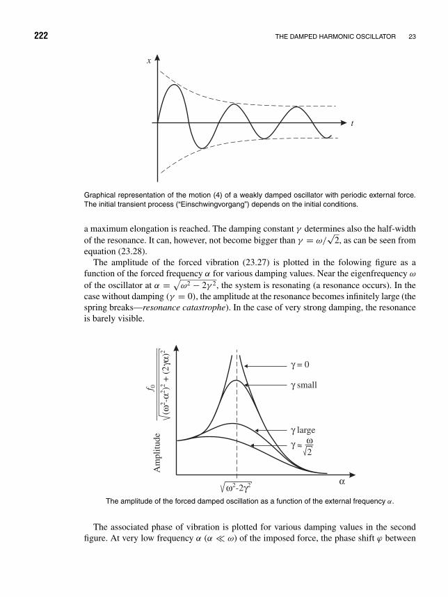
222 THE DAMPED HARMONIC OSCILLATOR 23
x
t
Graphical representation of the motion (4) of a weakly damped oscillator with periodic external force.The initial transient process (“Einschwingvorgang”) depends on the initial conditions.
a maximum elongation is reached. The damping constant γ determines also the half-widthof the resonance. It can, however, not become bigger than γ = ω/
√2, as can be seen from
equation (23.28).The amplitude of the forced vibration (23.27) is plotted in the folowing figure as a
function of the forced frequency α for various damping values. Near the eigenfrequency ω
of the oscillator at α = √ω2 − 2γ 2, the system is resonating (a resonance occurs). In the
case without damping (γ = 0), the amplitude at the resonance becomes infinitely large (thespring breaks—resonance catastrophe). In the case of very strong damping, the resonanceis barely visible.
γ = 0
γ small
γ large
γ ~~
α
Am
plitu
def 0
(-
)+
(2
)ω
αγα
22
22
ω γ2 2-2
ω2
The amplitude of the forced damped oscillation as a function of the external frequency α.
The associated phase of vibration is plotted for various damping values in the secondfigure. At very low frequency α (α ω) of the imposed force, the phase shift ϕ between
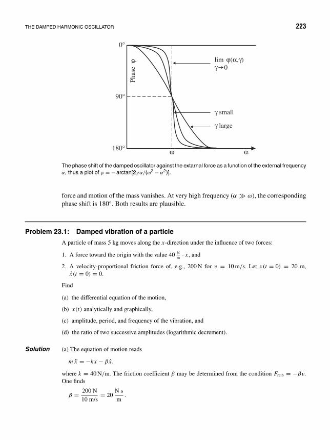
THE DAMPED HARMONIC OSCILLATOR 223
Phas
eϕ lim ( , )
0ϕ α γ
γ
γ small
γ large
ω α
0
90
180
°
°
°
The phase shift of the damped oscillator against the extarnal force as a function of the external frequencyα, thus a plot of ϕ = − arctan[2γα/(ω2 − α2)].
force and motion of the mass vanishes. At very high frequency (α ω), the correspondingphase shift is 180. Both results are plausible.
Problem 23.1: Damped vibration of a particle
A particle of mass 5 kg moves along the x-direction under the influence of two forces:
1. A force toward the origin with the value 40 Nm · x , and
2. A velocity-proportional friction force of, e.g., 200 N for v = 10 m/s. Let x(t = 0) = 20 m,x(t = 0) = 0.
Find
(a) the differential equation of the motion,
(b) x(t) analytically and graphically,
(c) amplitude, period, and frequency of the vibration, and
(d) the ratio of two successive amplitudes (logarithmic decrement).
Solution (a) The equation of motion reads
m x = −kx − β x,
where k = 40 N/m. The friction coefficient β may be determined from the condition Freib = −βv.One finds
β = 200 N
10 m/s= 20
N s
m.

224 THE DAMPED HARMONIC OSCILLATOR 23
By setting ω2 = k/m = 8 s−2, 2γ = β/m = 4 s−1, the equation of motion turns into
x + 2γ x + ω2x = 0
orx + 4x + 8x = 0.
(b) From ω2 = 8 s−2 and γ 2 = 4 s−2 it follows that ω2 > γ 2, that is, there is a weak damping. Thegeneral solution of the differential equation of a damped harmonic motion is given by 1
x(t) = exp (−γ t) [A cos(t) + B sin(t)] ,
where = √ω2 − γ 2 = 2 s−1. The constants A and B may be determined from the initial conditions:
x0 = x(t = 0) = A = 20 m,
x = −γ e−γ t (A cos(t) + B sin(t)) + e−γ t (−A sin(t) + B cos(t)) ,
x(t = 0) = 0 = −γ x0 + B, B = x0γ
= x0 = 20 m.
Hence
x(t) = 20 (cos t + sin t)e−γ t m. (23.29)
Because
A cos t + B sin t =√
A2 + B2 cos(t − ϕ),
with
tan ϕ = B
A,
for x(t) it results that
x(t) = 20√
2 cos(t − π
4
)e−γ t m
or
x(t) = 20√
2e−γ t cos(t − π
4
)m.
When setting x(t) = 0, we obtain a necessary condition for extrema: t = kπ/2 s, with k an integernumber. The zeros follow from cos(t − π
4 ) = 0. Thus, we get the following table:
t 03π
8= 1.18
π
2= 1.57
7π
8= 2.75 π = 3.14
11π
8= 4.32
x(t) 20 0 −0.86 0 0.04 0
Obviously this vibration is damping out rapidly. Actually, the parameters γ = 2/s and ω = √8/s
are close before the critical damping.(c) I. The amplitudes are therefore
a(t) = 20√
2e−γ t m.
1Here we use a frequently adopted notation for the exponential function: exp(x) ≡ ex .

THE DAMPED HARMONIC OSCILLATOR 225
x
20
15
10
5
0
–21 2 3 4 t
The solution function.
II. The frequency is
= √ω2 − γ 2 = 2 s−1.
III. For the period, it results that
T = 2π1
= π s.
(d) For two successive maximal elonga-tions, we obtain
xn = 20√
2e−γ t m,
xn+1 = 20√
2e−γ (t+2π/) m,
from which it follows that
xn
xn+1= eγ T
(where T = 2π
).
Therefore,
ln
(xn
xn+1
)= γ T (23.30)
is the logarithmic decrement. The meaningof this quantity is due to the fact that according to equation 23.30 the damping constant γ may bedetermined directly by measuring the ratio of successive maximal elongations.
Problem 23.2: The externally excited harmonic oscillator
(a) An oscillator with the eigenfrequency ω be undamped and excited by a harmonic external forceof the same frequency ω (e.g., by a balance wheel). The amplitude of the oscillator then increasesas a function of time according to the equation
x = A cos ωt + B sin ωt + f0t
2ωsin ωt.
Check that!
(b) Give a physical interpretation!
Solution (a) The force law reads
md2x
dt2= −kx − β
dx
dt+ F0 cos αt
and there must be β = 0 because the oscillator shall be undamped. By rewriting it follows that
x + ω2x = f0 cos αt, where α = ω and ω2 = k
m. (23.31)
To get the general solution of the equation, we add to the general homogeneous solution, that is, tothe solution of
x + ω2x = 0 , (23.32)

226 THE DAMPED HARMONIC OSCILLATOR 23
a particular solution of 23.31. The general solution of 23.32 now reads
x = A cos ωt + B sin ωt. (23.33)
It is convenient to adopt the following ansatz for the particular solution:
x = t (C1 cos ωt + C2 sin ωt). (23.34)
Here C1 and C2 are so far unknown coefficients. Differentiation yields
x = t (−ωC1 sin ωt + ωC2 cos ωt) + (C1 cos ωt + C2 sin ωt) (23.35)
andx = t
(−ω2C1 cos ωt − ω2C2 sin ωt)+ 2(−ωC1 sin ωt + ωC2 cos ωt). (23.36)
We insert equations (23.34), (23.35), and (23.36) in (23.31) and obtain after simplifying
−2ωC1 sin ωt + 2ωC2 cos ωt = f0 cos ωt.
From there it follows that C1 = 0 and C2 = f0/2ω. Thus the particular solution 23.34 reads
x = f0
2ωt sin ωt. (23.37)
x
t
Amplification of an externally drivenoscillator.
The general solution then reads
x = A cos ωt + B sin ωt + f0
2ωt sin ωt. (23.38)
(b) The constants A and B are determined from the initialconditions. Because there is no damping, the terms propor-tional to A and B do not become small at large times. Butfor large times (t → ∞), the term proportional to t increasesbeyond any limits such that the spring finally will break. Adrawing of the latter term shows the increase of the vibrationamplitudes with time: This is the typical case of “amplifica-tion” of a vibration as is well known from everyday life, forinstance, on swinging, periodic pulling of a cut-in tree to causeits breaking, etc.
Problem 23.3: Mass point in the x , y-plane
A mass moves in the x, y-plane. In the x-direction the harmonic force Fx = −mω2x and the additionalforce Kx = αmω2 y (α > 0) act, in the y-direction only the harmonic force Fy = −mω2 y acts.
(a) Solve the equations of motion with the initial conditions
x(0) = y(0) = 0, x(0) = 0, y(0) = Aω.
(b) Draw a qualitative figure of the path of the mass point.
Solution (a) The equations of motion read
mx = −ω2mx + αmω2 y,
x = −ω2(x − αy), (23.39)
andy = −ω2 y. (23.40)
THE DAMPED HARMONIC OSCILLATOR 227
Equation 23.40 is solved by the general ansatz
y(t) = a sin ωt + b cos ωt .
The initial conditions yield
y(0) = b = 0, y(0) = aω = Aω.
Hence the solution for y(t) reads
y(t) = A sin ωt. (23.41)
For 23.39 we then get with the help of 23.41
x = −ω2(x − αA sin ωt). (23.42)
We guess a particular solution of the inhomogeneous equation
xs(t) = ct cos ωt,
xs(t) = −2cω sin ωt − cω2t cos ωt,!= −ω2ct cos ωt + αAω2 sin ωt
⇒ −2c = αAω, c = −αAω
2.
The general solution of 23.42 is then
x(t) = d cos ωt + e sin ωt − αAω
2t cos ωt. (23.43)
The initial conditions yield
x(0) = d = 0, x(0) = eω − αAω
2= 0
⇒ e = αA
2.
Hence, the solution of the equations of motion reads
x(t) = αA
2[sin ωt − ωt cos ωt] ,
y(t) = A sin ωt.
(b) In the y-direction one obviously observes a harmonic vibration with amplitude A:
y(t An
) = ±A for t An = (2n + 1)π
2ω, n = 0, 1, 2, . . . .
The associated x-coordinate reads
x(t An
) = ±αA
2.
The zero passages of y are obtained from
y(t0n
) = 0 for t0n = nπ
ω, n = 0, 1, 2, . . . (23.44)
⇒ x(t0n
) = −αA
2nπ(−1)n . (23.45)

228 THE DAMPED HARMONIC OSCILLATOR 23
The motion of the particle is shown in the following figure.
x
yA
–A
– /2A α
A /2α
The motion of the particle. The path of the particle is stretching more and more in a cigar shape alongthe x-direction, while its width approaches the maximum value 2A.

24 The Pendulum
A mass m vibrating in a plane, suspended on a string of length l (let the mass of the string benegligibly small), is called a mathematical pendulum. The vibration period of the pendulumshall be calculated.
(a) Without damping
ϕ
l
Sm
ϕmg
FR
The pendulum: S gives thelenght of the arc, FR the act-ing force.
The backdriving force FR after displacing the mass by theangle ϕ is the component of the earth attraction along thedirection of motion of the pendulum
FR = −mg sin ϕ.
Hence, the differential equation for the pendulum withoutdamping is
ms = −mg sin ϕ,
s + g sin ϕ = 0,
s = lϕ,
s = lϕ,
lϕ + g sin ϕ = 0,
ϕ + g
lsin ϕ = 0,
ϕ + ω2 sin ϕ = 0. (24.1)
This differential equation is nonlinear. Howver, for small angles ϕ the sine of the anglecan be replaced by the angle itself, that is, for ϕ 1 we can use sin ϕ = ϕ. The differentialequation for the pendulum vibration for small displacements thus reads
ϕ + ω2ϕ = 0.
229

230 THE PENDULUM 24
This is a linear differential equation. Its general solution is
ϕ = A cos ωt + B sin ωt, ω =√
g
l,
from which we get the vibration period
T = 2π
ω= 2π
√l
g. (24.2)
(b) Vibration of the pendulum with friction but for small elongations
The differential equation reads
ms = −mg sin ϕ − β s.
The last term −β s represents the friction force. After division by m · l and by 2γ =β/(ml), we have
ϕ + ω2 sin ϕ + 2γ ϕ = 0. (24.3)
For small vibration amplitudes this turns into
ϕ + ω2ϕ + 2γ ϕ = 0.
The general solution is now (compare to Chapter 23)
ϕ =(
A cos√
ω2 − γ 2 t + B sin√
ω2 − γ 2 t)
e−γ t (weakly damped vibration),
or
ϕ =(
Ae−√
γ 2−ω2t + Be√
γ 2−ω2 t)
e−γ t (strong damping),
orϕ = (At + B)e−γ t (critical damping).
In all of these cases the pendulum comes to rest at some time (t → ∞).
(c) Solution of the pendulum equation without friction, but for large elongations
We begin with the nonlinear differential equation (24.1)
d2ϕ
dt2+ ω2 sin ϕ = 0
and substitute the angular velocity u = dϕ/dt :
du
dϕ· dϕ
dt+ ω2 sin ϕ = 0, hence u
du
dϕ+ ω2 sin ϕ = 0.

THE PENDULUM 231
Separation of the variables and integration yield∫u du = −
∫ω2 sin ϕ dϕ or
u2
2= ω2 cos ϕ + C.
With the boundary condition that for ϕ = ϕ0, u = 0, we obtain
0 = ω2 cos ϕ0 + C, C = −ω2 cos ϕ0,
oru2
2= ω2(cos ϕ − cos ϕ0),
dϕ
dt= u = √
2ω√
cos ϕ − cos ϕ0.
Another separation of variables and integration yield
ϕ∫ϕ1
dϕ√cos ϕ − cos ϕ0
=∫ √
2ω dt = √2ωt .
ϕ1 is an arbitrary initial angle. It is determined such that for t = 0 we get ϕ = 0. Thismeans
t = +√
l
2g
ϕ∫0
dϕ√cos ϕ − cos ϕ0
, (24.4)
and in particular
T
4= +
√l
2g
ϕ0∫0
dϕ√cos ϕ − cos ϕ0
or
T = 4
√l
2g
ϕ0∫0
dϕ√cos ϕ − cos ϕ0
. (24.5)
To evaluate the integrals (24.4, 24.5), we substitute cos ϕ = cos(ϕ/2 + ϕ/2) = cos2 ϕ/2 −sin2 ϕ/2 = 1 − 2 sin2 ϕ/2, which yields
T = 4
2
√l
g
ϕ0∫0
dϕ√− sin2 ϕ/2 + sin2 ϕ0/2.
The further substitution of
sinϕ
2= sin
ϕ0
2sin φ

232 THE PENDULUM 24
means a stretching of the variable ϕ that varies between 0 ≤ ϕ ≤ ϕ0 over the range0 ≤ φ ≤ π/2. Then
cos φ =√
1 − 1
sin2 ϕ0/2sin2 ϕ/2 . (24.6)
Furthermore, we have
1
2cos
ϕ
2dϕ = sin
ϕ0
2cos φ dφ,
and therefore
dϕ = 2 sin ϕ0
2 cos φ dφ√1 − sin2 ϕ0
2 sin2 φ.
With the abbreviation k2 = sin2 ϕ0/2, we get
T = 2
√l
g·
π/2∫0
2 sinϕ0
2cos φ dφ
√1 − k2 sin2 φ ·
√sin2
ϕ0
2
(1 − 1
sin2 ϕ0
2
sin2 ϕ
2
) ,
or according to (24.6)
T = 4
√l
g
π/2∫0
cos φ dφ
(√
1 − k2 sin2 φ) cos φ= 4
√l
g
π/2∫0
dφ√1 − k2 sin2 φ
.
For
ϕ0 π
2⇒ T = 4
√l
g
π/2∫0
dφ = 2π
√l
g,
that is, for small pendulum elongations the result known from equation (24.2) is reproduced.For larger elongations φ, the equation for the vibration period T with x(φ) = −k2 sin2 φ
reads
T = 4
√l
g
π/2∫0
dφ√1 + x(φ)
. (24.7)
This is an elliptic integral. Such types of integrals arise, for example, on calculating thearc length of an ellipse, which explains the name. It may be evaluated approximately byexpansion. Using the general binomial theorem
(1 + x)p = 1 +(
p
1
)x +
(p
2
)x2 +
(p
3
)x3 + · · · ,

THE PENDULUM 233
thus
(1 + x)p = 1 + px + p(p − 1)x2
1 · 2+ p(p − 1)(p − 2)x3
1 · 2 · 3+ · · · ,
which may also be proved by means of a Taylor expansion (Chapter 22), follows for1/
√1 + x , which may also be written as (1 + x)−1/2:
(1 + x)−1/2 = 1 +(
−1
2x
)+ −1/2(−3/2)
2x2 + · · · ,
(1 + x)−1/2 = 1 − 1
2x + 3
8x2 − · · · ,
(1 − k2 sin2 φ)−1/2 = 1 + 1
2k2 sin2 φ + 3
8k4 sin4 φ + · · · ,
T = 4
√l
g
π/2∫0
(1 + 1
2k2 sin2 φ + 3
8k4 sin4 φ + · · ·
)dφ.
By using the recursion formula∫sinm x dx = − 1
msinm−1 x · cos x + m − 1
m
∫sinm−2 x dx for m = 0,
which is obtained by partial integration, we obtain
π/2∫0
sin2n ϕ dϕ = 1 · 3 · 5 · . . . (2n − 1)
2 · 4 · 6 . . . (2n)· π
2.
Then we get for the vibration period
T = 4
√l
g
[π
2+ 1
2k2 π
4+ 3
8k4 3
8
π
2+ · · ·
]or
T = 2π
√l
g
[1 + 1
4k2 + 9
64k4 + · · ·
].
With k2 = sin2 ϕ0/2, this expression finally turns into
T ≈ 2π
√l
g
[1 + 1
4sin2 ϕ0
2+ . . .
]
= T0
(1 + 1
4sin2 ϕ0
2+ . . .
), where T0 = 2π
√l
g.
If ϕ0 1, we obviously obtain the old formula. If ϕ0 becomes larger, the vibrationperiod increases over T0. This is plausible as the backdriving forces are ∼ sin ϕ. Harmonic

234 THE PENDULUM 24
approximation means sin ϕ ≈ ϕ. For larger ϕ the backdriving forces become smaller than∼ ϕ, and therefore T > T0.
Problem 24.1: The cycloid
A circle of radius a rolls on a straight line. A given point on this circle then performs a cycloid. Findthe parameter representation of this cycloid.
2a
y P Ma
at
0 x xARolling a circle yields a cycloid.
Solution One has (see figure)
O A = a · t, O A = x + a sin t,
a = y + a cos t,
and therefore,
x = at − a sin t, y = a − a cos t,
x = a(t − sin t), y = a(1 − cos t).
This is the wanted parameter representation of the cycloid. Elimination of t yields the trajectoryin x-y-representation,
x(y) = −√2ay − y2 + a arccos
(a − y
a
).
Problem 24.2: The cycloid pendulum0
A CB
x
y
The string of the pendulum is warped alongthe two branches of the cycloid (gray). Themass m moves again on a cycloid.
In a vibration of a pendulum of mass m the stringshall osculate forth and back to the two branches O Aand OC of a cycloid (cycloid pendulum). The lengthof the string shall be half of the length of the cycloidbow.
Show that the curve ABC again is a cycloid.
Solution The equation of the cycloid branches reads
x = a(φ − sin φ), y = a(1 − cos φ).
The equation of the curve generated by the pendulum is
x = x1 + x, x1 = a(φ1 − sin φ1), (24.8)
y = y1 + y, y1 = a(1 − cos φ1).
(Equation of the cycloid. φ1 is the curve parameter of the cycloid point where the string lifts offfrom the osculation curve.)
Moreover,
(y)2 + (x)2 = l21 and l1 = l − s1. (24.9)
The calculation of s1 runs as follows:(ds
dφ
)2
=(
dx
dφ
)2
+(
dy
dφ
)2

THE PENDULUM 235
= a2[(1 − cos φ)2 + sin2 φ
]= a2
[1 − 2 cos φ + cos2 φ + sin2 φ
]= 2a2(1 − cos φ),
s1∫0
ds =φ1∫
0
a√
2√
(1 − cos φ) dφ.
Moreover, we set 1 − cos φ = 2 sin2 φ
2 , φ
2 = z, hence dzdφ
= 12 , and dφ = 2 dz. We then obtain
s1 = −4a cosφ
2
∣∣∣∣φ1
0
= 4a
(1 − cos
φ1
2
).
Hence, the total length of the cycloid bow is 8a, and therefore the string length is l = 4a and
x
y
x1
y1
l1
s1
∆x
α
∆y
x x1+∆
y y1+∆
The determination of x .
l1 = l − s1 (equation 24.9), that is,
l1 = 4a cosφ1
2. (24.10)
To get the equation of the trajectory of the vibrating mass,we now need the quantity x according to equation 24.9. Itholds that (see figure)
tan α = dy1
dx1
= = sin φ1
1 − cos φ1
= = sin φ1
2 sin2 φ1/2,
and therefore
x = l1 cos α = 4a cosφ1
2· 1√
1 + tan2 α= 4a cos
φ1
2sin
φ1
2.
The quantity y is calculated in a similar way, namely
y = l1 sin α = 4a cosφ1
2
tan α√1 + tan2 α
= 4a cosφ1
2cos
φ1
2= 4a cos2 φ1
2.
From there the x- and y-coordinates of the path result according to equation 24.8 as
x = x1 + x = a
[(φ1 − sin φ1) + 4 sin
φ1
2cos
φ1
2
]and because
1
2sin φ1 = cos
φ1
2sin
φ1
2,
x = a[φ1 + sin φ1],
x = a[φ1 − sin(φ1 + π)],

236 THE PENDULUM 24
y = y1 + y = a
[(1 − cos φ1) + 4 cos2 φ1
2
]= a [(1 − cos φ1) + 2(cos φ1 + 1)] ,
y = a[3 + cos φ1] = a[1 − cos(φ1 + π) + 2],
y = a[1 − cos(φ1 + π)] + 2a.
The trajectory of the vibrating mass again is a cycloid, namely
x = a[(φ1 + π) − sin(φ1 + π)] − πa,
y = a[1 − cos(φ1 + π)] + 2a.
It has the same form as the branches of the generating cycloid. The pendulum, however, is shiftedwith respect to the generating cycloid branches, namely by 2a in the y-direction, and by −aπ inthe x-direction. Thus, one may ensure by this simple construction that a mass suspended by a stringvibrates along a cycloid. Such a pendulum is called a cycloid pendulum.
Problem 24.3: A pearl slides on a cycloid
A pearl of mass m is forced to slide down on a frictionless wire with the contour of a cycloid. Let thepearl start from the rest position x = y = 0. The wire hangs in the gravitational field near the earth’ssurface (compare figure).
(a) Calculate the velocity of the pearl at the point y = 2a.
(b) Show that the vibration period of this motion equals that of a pendulum of length 4a.
mx
y
2a
g (GravitationalAcceleration)
Motion of a pearl along a cycloid.
Solution (a) According to the energy law, the balance for an arbitrary point P on the wire reads as follows:
Epot(P) + Ekin(P) = Epot(0, 0) + Ekin(0, 0),
that is,
mg(2a − y) + 1
2m
(ds
dt
)2
= mg(2a) + 0
or
2mga − mgy + 1
2mv2 = 2mga
orv2 = 2gy

THE PENDULUM 237
and finally,
v = √2gy.
We ask for the velocity v at the position y = 2a:
v(2a) = √2g · 2a = √
4ga = 2√
ga.
This result is so far independent of the special curve of the wire.(b) From the first part of the problem ⇒ (ds/dt)2 = 2gy.The square of velocity along the cycloid reads(
ds
dt
)2
=(
dx
dt
)2
+(
dy
dt
)2
= a2(1 − cos β)2β2 + a2 sin2 β · β2 = 2a2(1 − cos β)β2,
because the cycloid is given by x = a(β − sin β), y = a(1 − cos β). Therefore,
2a2(1 − cos β)β2 = 2ga(1 − cos β),
namely
β2 = g
a⇒ β = dβ
dt=√
g
a⇒ β = t
√g
a+ C1.
The last step is performed by integration after separating the variables. The initial conditions areβ = 0 for t = 0, β = 2π for t = T/2, T period of vibration. Therefore T = 4π
√a/g =
2π√
4a/g.By comparison with the formula for the simple pendulum, we find
Tpendulum = 2π
√l
gand Tcycloid = 2π
√4a
g⇔ l = 4a .
Problem 24.4: The search for the tautochrone
y
xS
The quantities used to find the tautochrone.
The problem of the tautochrone1 is thesearch for that curve for which the vibra-tion period is independent of the elonga-tion: Which trajectory must be passed bya mass point m to ensure that the vibrationperiod T of a frictionless vibrational mo-tion becomes independent of the value ofthe initial elongation h?
Solution Let s be the arc length on the wanted tau-tochrone (see figure). With v = ds/dt ,the energy law yields for the initial position and an arbitrary intermediate position
m
2
(ds
dt
)2
+ mgy = mgh,
1Greek: tautos chronos = equal time.

238 THE PENDULUM 24
orm
2
(ds
dt
)2
= mg(h − y),
from which, using
ds = ds
dydy = s ′(y) dy,
after separation of the variables it follows that
dt = 1√2g
s ′(y) dy√h − y
,
or after integration along a quarter of vibration
1
4T = 1
4T (h) = 1√
2g
h∫y=0
s ′(y) dy√h − y
,
and with the transformation y/h = u
T (h) =√
8
g
1∫0
s ′(hu)√
h du√1 − u
. (24.11)
Here T obviously is still a function of the parameter h occuring under the integral. In the sense of theformulated problem (T = constant) we now have to require
dT (h)
dh= 0 =
√8
g
1∫0
d
dh
[s ′(hu)
√h√
1 − u
]du =
√8
g
1∫0
√h · us ′′(hu) + 1
2√
hs ′(hu)
√1 − u
du .
This is definitely fulfilled if the numerator of the integrand vanishes, that is, if the differential equation
2hus ′′(hu) + s ′(hu) = 0 = 2ys ′′(y) + s ′(y)
ors ′′(y)
s ′(y)= − 1
2y(24.12)
is fulfilled. Now
s ′′(y)
s ′(y)
= d
dy[ln s ′(y)] and − 1
2y= d
dyln
√C1
y.
Hence from 24.12 it follows that
d
dy
[ln s ′(y) − ln
√1
y− ln
√C1
]= 0
or after integration
ln s ′(y) = ln
√C1
yor s ′(y) =
√C1
y.

THE PENDULUM 239
From 24.12 it follows with ds = √1 + (dx/dy)2 dy = (ds/dy)dy = s ′(y) dy, hence
√C1/y =√
1 + (dx/dy)2 , from which after separation of variables
dx =√
C1
y− 1 dy = √
C1 y − y2dy
y,
and after integration with the new integration constant C2 it finally results in
x =∫ √
C1 y − y2dy
y
= √C1 y − y2 − C1
2arccos
2y − C1
C1+ C2 . (24.13)
We check: With
f = √C1 y − y2,
it follows that
f ′(y) = C1 − 2y
2√
C1 y − y2,
and with
g(y) = arccos
(2y − C1
C1
),
it follows that
g′(y) = − 2
C1
√1 −
(2y − C1
C1
)2= − 2√−4y2 + 4yC1
= − 1√C1 y − y2
,
such that in fact(f (y) − C1
2g(y)
)′= C1 − 2y
2√
C1 y − y2+ C1
2√
C1 y − y2= C1 − y√
(C1 − y)y=√
C1 y − y2
y.
Hence, the curve 24.13 is a cycloid (compare to Problem 24.1). This result becomes even moreobvious if we determine the integration constants C1 and C2 from the boundary conditions y(x =0) = 0, y(x = πa) = 2a as C1 = 2a and C2 = aπ , so that for 24.13 it finally follows that
x = √2ay − y2 − a arccos
y − a
a+ aπ
= √2ay − y2 + a
(π − arccos
y − a
a
).
We still check the vibration period, using 24.11. With s ′(y) = √C1/y = √
2a/y, we get accordingto 24.13:
T =√
8
g
h∫0
s ′(y) dy√h − y
=√
8
g
h∫0
√2a dy√
y(h − y)= 2
√4a
g
h∫0
dy√y(h − y)
,

240 THE PENDULUM 24
= −2
√4a
g· arcsin
(1 − 2y
h
)∣∣∣∣∣h
0
= 2π
√4a
g= 2π
√lr
g, (lr = 4a),
namely, actually a value that is independent of the initial elongation h. We shall prove the uniquenessof the solution in Vol. 2 of the lectures, after we have become familiar with the Fourier series.
a
y
x
2a
aπCycl.
Cycloid
Cyclo
id
The cyloid as the tautochrone (left), and used as jaws in Huygens’ construction of a pendulum whoseperiod does not depend on the amplitude (right).
Historical remark: The treatment of this problem may be traced back to Huygens,2 who aimed atthe construction of a pendulum, with the vibration period being independent of the amplitude. Becausethe evolvent of a cycloid again represents a cycloid, a cycloid string pendulum may be constructed byforcing the pendulum motion of the mass m into a cycloid trajectory by an appropriate assembly oftwo cycloid jaws (compare the figure and Problem 24.2). Such a construction was realized in 1839 bythe Austrian engineer Stampfer for the clock of the City Hall tower in Lemberg. This clock excelledby a very high accuracy of performance until its destruction by lightning.
2Christiaan Huygens, physicist and mathematician, b. April 14, 1629, Den Haag—d. there July 8, 1695. Afterfirst studying jurisprudence, he turned to mathematical research and published among others in 1657 a treatiseon probability calculus. At the same time he invented the pendulum clock. In March 1655 he discovered thefirst Saturn moon; in 1656 the Orion nebula and the shape of the Saturn ring. Already then he was also familiarwith the laws of collisions and those of central motion, but published them—without proofs—only in 1669.In 1663 Huygens became elected as member of the Royal Society. In 1665 he settled in Paris, as a memberof the newly founded French Academy of Sciences, from where he returned to the Netherlands in 1681. Afterpublishing his Systema Saturnium, sive de causis mirandorum Saturni phaenomenon already in 1657, his mainwork Horologium oscillatorium (The pendulum clock) emerged in 1673, which, besides the description of animproved clock construction, contains a theory of the physical pendulum. Also contained there are treatises onthe cycloid as an isochrone and important theorems on central motion and the centrifugal force. From 1675 datesHuygens’ invention of the spring watch with balance spring; from 1690 the Tractatus de lumine, the treatise onlight where a first version of the wave theory of double refraction of Iceland spar is developed. The sphericalpropagation of the action about the light source is explained there by means of Huygens’ principle. The Frenchedition of the Traite de la lumiere (Leiden, 1690) also includes a Discours de la cause de la pesanteur as asupplement [BR].

25 MathematicalInterlude:DifferentialEquations
On treating mechanical problems we became familiar with differential equations. An (or-dinary) differential equation is a relation between an independent variable (t), a functionx(t), and one or several of its derivatives (x, x, . . .) from which the wanted function x(t)shall be calculated. The differential equation is said to be of first order if only the first ofits derivatives is involved. Such a differential equation may be written as
F(t, x, x) = 0 (25.1)
or, when solving for x , as
x(t) = f (t, x). (25.2)
A differential equation is of second order if no higher derivative than the second one occurs.A differential equation of second order therefore has the form
F(t, x, x, x) = 0
or, resolved for x ,
x = f (t, x, x). (25.3)
The meaning of a differential equation of first order (25.2) is understood as follows: xdetermines the direction of the curve x(t) in the t, x-plane. The differential equation (25.2)assigns a direction to any point t, x ; it defines a direction field. We may visualize this field,for example, by plotting in a sufficiently dense lattice of points t, x the direction at eachlattice point by a short dash (see the figure). The differential equation is solved by plottingcurves into this direction field; the directions of these curves at any point correspond to the
241

242 MATHEMATICAL INTERLUDE: DIFFERENTIAL EQUATIONS 25
direction field. If f (t, x) is a reasonable function, one may interpolate between the plotteddirections in the direction field. In this way one obtains a set of curves. In other words: Thedifferential equation (25.2) allows a set of solving functions x(t). An individual curve ofthe set is specified by prescribing the value of x belonging to a fixed value of t (in the figure,the value x0 for t = 0). Such a set of curves in which the individual curve is determined bya single number (a parameter) is called a one-parametric set of curves. We therefore maystate:
x
t
x0
Direction field of a differen-tial equation of first order.
A differential equation of first order (25.2)—with a rea-sonable function f (t, x)—determines a one-parametric setof curves. The general solution contains an arbitrary integra-tion constant (x(0) = x0).
This also holds vice versa: To any (reasonable) one-parametricset of nonintersecting curves in the t, x-plane there corre-sponds a differential equation of first order. The curves of theset may namely be described by the equation
ϕ(t, x) = c , (25.4)
where c for each curve takes a distinct value. The function ϕ is not uniquely determined bythe set of curves, as any possible function ϕ may be replaced by a function of ϕ, that is, byF(ϕ) = F(c) = C and nevertheless describes the same set of curves. For the direction ofthe curves it follows that
∂ϕ
∂tdt + ∂ϕ
∂xdx = 0, (25.5)
or (assuming ∂ F/∂ϕ = 0)
∂ F
∂ϕ
(∂ϕ
dtdt + ∂ϕ
∂xdx
)= 0 ⇒ ∂ϕ
∂tdt + ∂ϕ
∂xdx = 0, (25.6)
that is, always the relation (25.5). From this relation it then follows that
x = − ϕt (t, x)
ϕx (t, x)≡ f (t, x), (25.7)
where ϕt and ϕx denote the partial derivatives with respect to t and x , respectively. If ϕ
is replaced by a function of ϕ, we obtain according to (25.6) the same equation (25.7).A one-parametric set of curves therefore essentially corresponds to a single differentialequation of first order. We therefore may state: A one-parametric set of curves (25.4) isequivalent to a differential equation. Particularly simple differential equations of first orderare of the type
x = f (t) (25.8)
andx = f (x). (25.9)

MATHEMATICAL INTERLUDE: DIFFERENTIAL EQUATIONS 243
In these cases the direction field depends only on one of the variables t or x , respectively.The solution of (25.8) may be obtained immediately:
x(t) =t∫
0
f (t ′) dt ′ + x0. (25.10)
Obviously all solutions originate from a single solution by adding an arbitrary constantto x(t) (by shifting the solution curves along the x-direction). The solution of (25.9) isobtained via the transformation
dt = dx
f (x)(25.11)
by the integral
t (x) =x∫
0
dx ′
f (x ′)+ t0. (25.12)
In this case all solutions are generated from a single (fixed) solution by adding an arbitraryconstant to t (by shifting the solution curve in the t-direction). A differential equation offirst order may be solved easily also then if it may be put into the form
g(x) dx = h(t) dt, (25.13)
that is, if the variables may be separated. We then get
x∫x0
g(x ′) dx ′ =t∫
0
h(t ′) dt ′. (25.14)
We now turn to the discussion of a differential equation of second order. The functionf (t, x, x) in (25.3) ascribes to each point t, x and to each given direction (x) throughthis point a defined change of direction. For a reasonable function f (t, x, x), we may findgraphical solutions as follows: We begin at an arbitrary point of the t, x-plane with anarbitrary direction of the curve, and then calculate the associated value of x accordingto (25.3). The curve is then continued as a parabola in the assumed direction (x) with thecalculated value of x (a parabola with a vertical axis has the same value of x everywhere).After a certain piece of continuation we have a new point t, x and a new direction x . Therewe again calculate x according to (25.3) and continue the curve by the corresponding newparabola, etc. The solution curve obtained this way depends on the choice of the positionand direction when starting the procedure. In total, we obtain an entire set of solutions. Theindividual solution curve is thus determined by specifying two numbers, for example, thevalues of x and x at a certain time point (t-value). A set of curves in which the individualcurve is determined by giving two numbers is called a two-parametric set of curves (seefigure). Thus we may state:
A differential equation of second order (25.3) with a reasonable function f (t, x, x)
determines a two-parametric set of curves.

244 MATHEMATICAL INTERLUDE: DIFFERENTIAL EQUATIONS 25
The general solution contains two arbitrary integration constants.Particularly simple differential equations of second order (which we met already) are
x = f (t), (25.15)
x = f (x), (25.16)
x = f (x). (25.17)
x
t
Set of solutions of a differ-ential equation of secondorder.
In the first case, (25.15), the acceleration is given as a func-tion of time; in the second case, (25.16), the acceleration isgiven as a function of the velocity; and in the third case, (25.17),as a function of the position. (25.15) may be solved by a twofoldintegration. (25.16) is of first order in x , thus it may be rewrittenwith v = x into v = f (v) and may then be solved as (25.9).(25.17) is transformed to
x x = f (x)x,
x d x = f (x) dx, (25.18)
1
2x2 =
x∫x0
f (x ′) dx ′ + c ,
and we thereby obtain a differential equation
x = ϕ(x),
which may be solved as (25.9). In physics the linear differential equations are of particularimportance because the phenomena described by these equations obey the superpositionprinciple (compare equations (21.4) and (21.5) ff.). We shall outline this point of view fora differential equation of second order; the reader may extend that to other orders. Thedifferential equation is linear if x, x, x occur linearly, that is, if the equation has the form
Ax + Bx + Cx + D = 0, (25.19)
where A, B, C, D may be functions of t . If the term D is missing, the equation is calledhomogeneous. If x1(t) solves a homogeneous linear differential equation, then cx1 with cbeing a constant is also a solution. If x1(t) and x2(t) are solutions, then c1x1 + c2x2 witharbitrary constants c1 and c2 is also a solution (compare equations (21.4) and (21.5) ff.).Because the general solution of a differential equation of second order contains two andonly two arbitrary constants, a homogeneous linear differential equation of second orderhas been solved generally if two distinct (linearly independent) solutions are known. If weknow a solution x1(t) of an inhomogeneous linear differential equation (25.19), that is,
Ax1(t) + Bx1(t) + Cx1(t) + D = 0, (25.20)
and if x0(t) is a solution of the homogeneous equation that arises by omitting the term D,that is,
Ax0(t) + Bx0(t) + Cx0(t) = 0 , (25.21)
MATHEMATICAL INTERLUDE: DIFFERENTIAL EQUATIONS 245
then (x0 + x1) is again a solution of equation (25.19). We have namely
A(x0 + x1) + B(x0 + x1) + C(x0 + x1) + D
= Ax0 + Bx0 + Cx0︸ ︷︷ ︸=0
+ Ax1 + Bx1 + Cx1 + D︸ ︷︷ ︸=0
= 0.
Hence, an inhomogeneous linear equation is solved generally if one has solved generally thehomogeneous equation and then adds a particular solution of the inhomogeneous equation.We have already used this statement in the context of the forced vibration (Chapter 23).One may convince oneself by means of (25.20) that two possibly distinct solutions of theinhomogeneous differential equation, x1(t) and x2(t), must be equal to each other, apartfrom a solution of the homogeneous equation (25.21). From Ax1 + Bx1 + Cx1 = −D =Ax2 + Bx2 + Cx2, it follows namely that
Ax1 + Bx1 + Cx1 = Ax2 + Bx2 + Cx2;hence
A(x1 − x2)·· + B(x1 − x2)
· + C(x1 − x2) = 0,
that is, the difference x1 − x2 of the two particular solutions must be a solution of thehomogeneous equation. Homogenous linear equations with constant coefficients (A, B, C)
are solved by means of the ansatz
x(t) = eλt .
From the differential equation
Ax + Bx + Cx = 0
results the algebraic equation (it is called characteristic equation)
Aλ2 + Bλ + C = 0
for λ. Its two solutions yield, if they don’t just coincide, two solutions of the differentialequation and thus the general solution
x = c1eλ1t + c2eλ2t .
If the quadratic equation in λ has only one solution, then
x = c1eλt + c2teλt
is the general solution of the differential equation, as may be checked easily (directly or bya limiting process).

26 Planetary Motions
In this chapter we shall investigate the motion in a central force field. As usual in physics, webegin with experimental observations—in our case the Kepler laws of planetary motion—and deduce the forces–in ur case the gravitational force between two masses. Later weshall reverse this process and start our reasoning with the forces and Newton’s equationsof motion, and we shall then derive Kepler’s laws, As will become evident, theory thenpredicts new phenomena not contained in Kepler’s laws, for example the orbits of comets,perhelion motion, and other facts.
Accordingsly, let us now consider in particular the planetary motion and start from thethree Kepler laws, which were derived by Johannes Kepler1 from the observations of planetsmade by Brahe.2 These three laws are as follows:
1Johannes Kepler, b. Dec. 27, 1571, Weil der Stadt—d. Nov. 15, 1630, Regensburg. Kepler was son of a traderwho often also served in military, first attended the school in Leonberg, and later the monastic school in Adelbergand Maulbronn. In 1589 Kepler began his studies in Tubingen, to become a theologian, but in 1599 he took theposition of professor of mathematics in Graz offered to him. In 1600 Kepler had to leave Graz, because of thecounterreformation, and he went to Prague. After the death of Tycho Brahe (Oct. 24, 1601) Kepler as his successorbecame imperial mathematician. After the death of his patron, emperor Rudolf II, Kepler left Prague and wentin 1613 to Linz as a land surveyor. From 1628 Kepler lived as employee of the powerful Wallenstein mostly inSagan. Kepler died fully unexpectedly during a visit to the meeting of electors in Regensburg.
Kepler’s main fields were astronomy and optics. After extraordinarily lengthy calculations he found thefundamental laws of planetary motion: the Kepler’s first and second laws were published 1609 in AstronomiaNova, the third one 1619 in Harmonices Mundi. In 1611 he invented the astronomical telescope. His RudolphianTables (1627) continued to be one of the most important tools of astronomy until the modern age. In the fieldof mathematics he developed heuristic infinitesimal considerations. His best-known mathematical writing is theStereometria Doliorum (1615) where, e.g., Kepler’s tub rule is given.
2Tycho Brahe, Danish astronomer, b. Dec. 14, 1546, Knudstrup on Schonen—d. Oct. 24, 1601, Prague. Hefirst studied law, secretly dealt with astronomy until he inherited a considerable fortune, and then continued hisstudy in Germany. In 1572 he became known by the discovery of a new star, the Nova Cassiopeiae, which was infact a supernova. He lectured in Copenhagen and, by recommendation by Wilhelm IV, count of Hessen-Kassel,who dealt with astronomy, he got the support of the Danish king Friedrich II, who in 1576 transferred to him theisland Ven in the Sound near Copenhagen. At the observatory “Uranienborg” built there Brahe dealt with researchand education and tutoring his numerous scholars and assistants. The troubles he met after the death of FriedrichII (1588) forced him to leave the country in 1597. After a two-year stay with the count Rantzau in Wandsbek nearHamburg, he served as imperial astronomer with Rudolf II. In Prague he again gathered a couple of coworkers,among them Christian Ljongberg (Longomontanus) and first of all Johannes Kepler.
246

PLANETARY MOTIONS 247
1. All planets are moving on ellipses. The sun stands in one of their focal points.
2. The radius vector sun–planet covers equal areas in equal times (area theorem).
3. The squares of the revolution periods of two planets are related to each other as thecubes of the large semi-axes of their trajectories.
θe1
e2
er
eθ
r
Unit vectors for Cartesian and polar co-ordinates.
Let us denote the large semi-axis by a and therevolution period of the th planet by T; then
T 21
a31
= T 22
a32
.
This means for a planet: T 2 ∼ a3.We adopt two approaches: First we try to find out
the properties of the force field from the Kepler laws.Later on we shall start from the force field that will beassumed to be given, and deduce the properties of thepath. In order to formulate the motion and the forcelaw, it is appropriate to formulate the equations ofmotion in polar coordinates. According to the first of Kepler’s laws, the motion must be aplanar motion.
We therefore introduce the local unit vectors er and eθ at each point. They are definedby the equations
er = cos θ e1 + sin θ e2,
eθ = − sin θ e1 + cos θ e2.
We know them already from Chapter 10 but shall briefly remind the essentials. The orien-tation of these unit vectors is time-dependent. Therefore,
er = (− sin θ e1 + cos θ e2)θ = θeθ ,
eθ = (− cos θ e1 − sin θ e2)θ = −θer .
We now express the velocity and acceleration in terms of these coordinates. Twofolddifferentiation yields
r = rer ,
r = rer + r er = rer + r θeθ ≡ v,
Brahe was the most significant observing astronomer before the invention of the telescope. He practicallyreached the possible accuracy of observations with the bare eye. The observations of Brahe and his coworkersformed the prerequisite for Kepler’s works on the orbits of planets. Brahe tried to substitute the Copernican worldsystem by his own system, according to which sun and moon are orbiting about the earth resting at the centerof the universe, while the remaining planets orbit about the sun. The Tychonian system was favored in the 17thcentury since the assumption of the incredibly large distances of the fixed stars that had to be presupposed byCopernicus were not needed in Brahe’s system. Brahe proved that the comets are not phenomena caused by theearth’s atmosphere, as was assumed, for example, by Aristotle [BR].

248 PLANETARY MOTIONS 26
v = rer + r er + r θeθ + r θeθ + r θ eθ
= (r − r θ2
)er + (
r θ + 2r θ)
eθ . (26.1)
The area theorem now reads simply
r2θ = h (h = constant). (26.2)
This may be seen as follows: Let the force center be at the coordinate origin; then
d A = |dA| = 1
2|r × dr|
is the infinintesimal area element, and furthermore
d A
dt= 1
2
∣∣∣∣r × drdt
∣∣∣∣ = 1
2|r × v| = 1
2h = constant , (26.3)
where 12 |r × v| is the “area velocity” of the radius vector. Hence:
|r × v| = r2θ = h.
From the area theorem found empirically by Kepler, it now follows that
d(r2θ )
dt= r(2r θ + r θ ) = 0.
A comparison with (26.1) yields for the wanted force field
r · eθ = 0, (26.4)
that is, no acceleration and hence no force is acting along the eθ -direction. The area theoremthus implies that we are dealing with a central force field. This is already known from earlier(Chapter 17). And vice versa, a central force field requires the area theorem to be valid: Forcentral forces the torque vanishes, D = r × F = 0. Hence, for central forces conservationof the angular momentum generally holds:
L = r × F = 0, L = −−−−→constant;
hence,
L = r × p = (r × v)m = −−−−→constant.
From there one may immediately derive
|L| = r2θm = hm . (26.5)
Mathematical interlude: consideration of conic sections in polar coordinates—ellipse, parabola, hyperbola:
The equation in polar coordinates
r = k
1 + ε cos θ(26.6)

PLANETARY MOTIONS 249
describes
circles (for ε = 0),
ellipses (for ε < 1),
parabolas (for ε = 1),
hyperbolas (for ε > 1).
Equation (26.6) is therefore the general equation for conic sections in polar coordinates.We make that clear in detail now:
y
xa
a a
c c
b
yr´
F´ r
F xθ
The geometry of the ellipse.
(a) Ellipse
It is the set of all points whose distances fromtwo fixed focal points F and F ′ in a distance of2c (see figure) have a constant sum 2a, which islarger than F F ′. Thus (compare figure), r + r ′ =2a, c2 + b2 = a2, where a and b are the majorand minor semi-axes of the ellipse, respectively.Further it holds that
c =√
a2 − b2 = ε · a, ε < 1.
ε is called eccentricity. For the circle ε = 0 (both focal points coincide, i.e., c = 0).Obviously (compare figure)
r +√
(2c)2 + r2 + 2(2c)r cos θ = 2a
or4ε2a2 + r2 + 4εar cos θ = (2a − r)2,
r = a(1 − ε2)
1 + ε cos θ≡ k
1 + ε cos θ,
where
k = a(1 − ε2) = a
(1 − a2 − b2
a2
)= b2
a2.
We still give the equation of an ellipse in Cartesian coordinates. From the figure one mayimmediately read off
r =√
(x − c)2 + y2, r ′ =√
(x + c)2 + y2 ,
such that the defining equation for the ellipse reads
r + r ′ =√
(x − c)2 + y2 +√
(x + c)2 + y2 = 2a .

250 PLANETARY MOTIONS 26
Forming twice the square, together with b2 = a2 − c2, then leads to
x2
a2+ y2
b2= 1.
(b) Circle
Circles casually fit in as special cases of ellipses (ε = 0).
(c) Parabola
The parabola is the geometric locus of all points P of a plane that have equal distance from
y
x
Guideline
c
c
dr
P
F θ
The geometry of the parabola.
the fixed guideline L and the fixed focal point F .Therefore,
r = d = 2c − r cos θ
or
r = 2c
1 + cos θ≡ k
1 + ε cos θ,
where ε = 1 and k = 2c. We shall also write theparabola in Cartesian coordinates. From the figure we read
r =√
(c + x)2 + y2 ,
such that from
r = d = c − x
after squaring follows
y2 = −4cx .
y
xa c
r´
F´
r
Fθ
The geometry of the hyperbola.
(d) Hyperbola
The hyperbola is the geometric locus of all points ofa plane whose distances from two fixed points on theplane (the focal points) F and F ′ (with distance 2c)have a constant difference. Hence
r − r ′ = 2a < F F ′
or
r −√
r2 + 4c2 + 4rc cos θ = 2a.

PLANETARY MOTIONS 251
With c = εa (ε > 1, see figure) it follows that
r = a(1 − ε2)
1 + ε cos θ≡ k
1 + ε cos θ, k = a(1 − ε2).
In Cartesian coordinates the hyperbola equation follows from the defining equation
r − r ′ = 2a
or√(c − x)2 + y2 −
√(c + x)2 + y2 = 2a
after squaring twice and using b2 = c2 − a2 as
x2
a2− y2
b2= 1.
Thus, the general form (26.6) of conical sections is founded.We now continue our physical considerations and return to the further investigation of
Kepler’s laws. In order to derive the special form of the force law from the Kepler laws, wenow take into account that the trajectory is an ellipse with the sun at one focal point. Theequation of the ellipse reads in polar coordinates
r = k
1 + ε cos θ, (26.7)
with the parameter
k = a(1 − ε2) = a2 1 − ε2
a= a2 − c2
a= b2
a,
and the eccentricity
ε =√
a2 − b2
a< 1 .
We already know from (26.4) that the force, and hence the acceleration, must be central,namely, proprtional to er . We thus can calculate the central acceleration—see (26.1)—andtaking into account (26.2), we get
r = dr
dθθ = ε
ksin θ r2θ = ε
kh sin θ,
r = ε
kh cos θ θ = εh2
kr2cos θ,
and, using (26.2) and (26.7) for the component of (26.1) along er , finally
r − r θ2 = h2
r2
(ε
kcos θ − 1
r
)= − h2
kr2. (26.8)

252 PLANETARY MOTIONS 26
The central force of the wanted field for a planet of mass m is therefore given by (seealso (26.1))
F(r) = m(r − r θ2)er = −h2
kr2m
rr.
At first the quantity h2/k appears as a constant that is specific for each planet. But keepingin mind the third Kepler law, we find that h2/k has the same value for all planets. Thismay be seen as follows: Because h/2 is the area velocity of the radius vector for a definedplanet, the area of the ellipse equals πab and b2 = ak, it follows for the revolution periodT that
h
2T = πab,
h · T = 2πab = 2π√
a3k,
andT 2
a3= 4π2k
h2⇒ h2
k= 4π2a3
T 2;
Because
a3
T 2= constant ⇒ h2
k= constant. (26.9)
Because according to the third Kepler law a3/T 2 is equal for all planets, the same obviouslyholds also for h2/k. The quantity h2/k is the same for all planets. Therefore, all planetsobey the force law
F(r) = − constantm
r2
rr.
If, according to the principle of actio and reactio, the mass of the central star is stillfactorized out from the constant (finally the force must vanish if the sun mass M vanishes),the gravitational law thus takes the form
F = −γMm
r2· r
r. (26.10)
It is remarkable how this fundamental force law may be deduced from Kepler’s laws. Aswe have seen, it is completely contained in these laws. Already Newton realized that theacceleration a planet feels due to the attraction by the sun is of the same nature as theacceleration on a freely falling body by the earth gravitation. The factor const = γ M in thelaw (26.10) is of course only then the same if the attracting body is the same in both cases,for example, the earth. Newton therefore compared the acceleration of fall near the earth’ssurface, roughly 10 m/s2, with the central acceleration of the moon on its orbit about theearth. The latter one is
ω2a = 4π2a
T 2= 40 · 6370 · 105 · 60
272 · 242 · 602 · 602
cm
s2,

PLANETARY MOTIONS 253
where the distance of moon a is set equal to 60 times the earth’s radius (6370 km), and thecirculation period of the moon equal to 27 days. Because
40 · 6370 · 102
272 · 242 · 60≈ 1,
it follows that
ω2a ≈ 103
602
cm
s2
andω2a / g ≈ 1 / 602;
that is, the acceleration of the moon on circulating about earth is actually related to theacceleration of free fall near the earth’s surface inversely as the squares of the distancesfrom the earth’s center.
Example 26.1: The Cavendish experiment
2l
Fiber
m1
m 1
m2
m 2Mirror
S
LightSource
Torsional balance for the determination ofthe gravitational constant.
In principle the gravitational constant γ may be de-termined by measuring the attractive force betweentwo bodies of known mass. In practice, however, thegravitational force is so weak that it becomes highlydifficult to demonstrate it in the laboratory. In theso-called Cavendish experiment (Cavendish,3 1798)the force between two masses is determined from thetorsion of an elastic suspension string (see figure).
The masses m1 and m ′1 are fixed to the ends of a
light scale beam of length 2l suspended by a very thinquartz fiber. Already a very weak force may force thefiber to rotate about its axis (torsion), such that thetorsion angle may provide a measure for very weakforces. To make the small torsion of the string visible,a mirror is attached to this string, which is hit by alight ray. Observation of the reflected ray allows usto measure any rotation of the string, and thus of themirror.
In the measurement of the gravitational constant γ two large masses m2 and m ′2 are positioned close
to the masses m1 and m ′1, as shown in the left figure below. Because of the gravitational attraction
the small masses m1, m ′1 move and thereby twist the string by the angle θ . After stabilization of this
configuration, within several hours the masses m2, m ′2 are brought into a new position, as represented
in the right figure below.
3Henry Cavendish, chemist, b. Oct. 10, 1731, Nizza—d. Feb. 28, 1810, London. He investigated gases indetail, isolated carbon dioxide and hydrogen as distinct kinds of gases (1766); he realized the composition of air,discovered the explosionlike combination of hydrogen and oxygen (oxyhydrogen gas) and hence the compositionof water. When working on nitrogen he discovered nitric acid. His determination of the gravitational constant bymeans of the torsional balance was of particular significance.

254 PLANETARY MOTIONS 26
b
b
F´
F´
θFF
The first position of the masses m2 andm′
2 for the determination of the gravi-tational constant.
F´F´
2θF
F b
The second position of the massesm2 and m′
2.
The string is now twisted anew by the gravitational force, namely in opposite direction by theangle 2θ . The system does not reach the final equilibrium state right now but rather oscillates withdecreasing amplitude toward the final position (weakly damped oscillator—see figure on the nextpage). The period of oscillation amounts to about 8 min, and after about 30 min the system reaches thefinal equilibrium state. From these data the force between the spheres is determined, and with knownmass and known distance between the centers of the spheres, we may calculate the gravitationalconstant γ from Newton’s gravitational law:
γ = 6.67 · 10−11 m3
kg s2 .
From the defining equation for the gravitational acceleration on the earth’s surface
g = γ · m E
R2E
(m E : mass of earth, RE : radius of earth)
and with the known constant γ we may now calculate the mass of earth. We obtain
m E = g · R2E
γ= 5.97 · 1024 kg,
where RE = 6.37 · 106 m, g = 9.81m/s2 have been assumed. This implies a mean mass density of
T=8.3 min
0 10 20 30 40 50 t (min)
60
50
44S0
Sd
EndPosition
Oscillations with weak dampening around the end position.

PLANETARY MOTIONS 255
earth of
= m
V= m E
43 π R3
E
≈ 5.5 · 103 kg
m3
or ≈ 5.5 g/cm3
((iron) = 7.86 g/cm3
).
Derivation of the Kepler laws from the force law
So far we have derived the gravitational law from the Kepler laws. Now we shall investigatecentral force fields in general. One may start from the assumption that the force field isknown. The central force field has the following properties:
1. Central force fields F = f (r) rr with arbitrary radial dependence f (r) are conservative,
that is, the energy conservation law is valid because
curl F =
∣∣∣∣∣∣∣∣∣∣∣
e1 e2 e3
∂
∂x
∂
∂y
∂
∂z
f (r)x
rf (r)
y
rf (r)
z
r
∣∣∣∣∣∣∣∣∣∣∣= 0.
With r = √x2 + y2 + z2 =
√x2
1 + x22 + x2
3 and ∂r/∂xi = xi/
√x2
1 + x22 + x2
3 = xi/rthere holds, for example, for the e1-component
∂
∂y
[f (r)
z
r
]− ∂
∂z
[f (r)
y
r
]= z
∂
∂r
(f (r)
r
)∂r
∂y− y
∂
∂r
(f (r)
r
)∂r
∂z
= ∂
∂r
(f (r)
r
)( zy
r− yz
r
)= 0.
The vanishing of the the other components can be deduced in an analogous way. This isalso vividly clear, as a central force field that points only toward the center or off centercannot have vortices.
2. If a body moves on an orbit in the central force field, then the orbital angular momentumis conserved. That means that the area theorem holds. For central force fields, we have
D = r × F = r × f (r)
rr = 0 = L;
thus
L = r × p = m(r × v) = −−−−→constant = mh
or1
2|r × v| = d A
dt= 1
2h = constant.

256 PLANETARY MOTIONS 26
3. A body in the central force field always moves in a plane, because from
r × v = h = −−−−→constant
it follows that
r · h = r · (r × v) = 1
mr · L = 0.
Hence, r points perpendicular to L. Because L is constant, r always lies in a plane. Inother words: The body moves only within a plane perpendicular to the angular momentumvector. Based on the conservation of energy E and of the angular momentum L, we shalltry to make statements on the orbital motion. The conservation laws concerning the angularmomentum and the energy according to (26.5) read
mr2θ = L , (26.11)1
2mv2 + V (r) = E (26.12)
with the gravitational potential
V (r) = −∫
F(r) · dr
= γ Mm
r∫∞
r · drr3
= γ Mm
r∫∞
dr
r2= −γ Mm
r.
The gravitational potential has been chosen such as to vanish at infinity (i.e., for r → ∞).This is always possible since we know that the potential is determined only up to an additiveconstant. Using
v2 = r2 + r2θ2,
we rewrite the energy conservation law (26.12) into
m
2(r2 + r2θ2) + V (r) = E .
With the angular momentum (26.11), it follows that
m
2r2 + L2
2mr2+ V (r) = E . (26.13)
Hence, the total energy is composed of three components: a radial kinetic energy (m2 r2);
a rotational energy (L2/2mr2); and a potential energy (V (r)). The rotational energy isusually written in the form L2/2J , where J = mr2 is the moment of inertia of the masspoint (the planet) with mass m when revolving at a distance r from the axis of rotation. Thiswill be treated in more detail in the second part of the mechanics course. From equation(26.13) we may now easily determine r(t), because
r =√
2
m(E − V (r) − L2/2mr2) , (26.14)

PLANETARY MOTIONS 257
dt = dr√2m (E − V (r) − L2/2mr2)
(separation of variables), (26.15)
t − to =r∫
r0
dr√2m (E − V (r) − L2/2mr2)
. (26.16)
As already mentioned, the total energy (26.13) consists of three terms; here 12 mr2 is
denoted as kinetic radial energy, and L2/2mr2 as rotational energy. This rotational energymay be incorporated into the potential, as L2 is constant and L2/2mr2 therefore acts like apotential term in (26.13). The term L2/2mr2 is therefore also called rotational potential orcentrifugal potential. Thus one is led to the effective potential
Veff = V (r) + L2
2mr2
consisting of the gravitational potential V (r) and the centrifugal potential L2/2mr2. From(26.11) we may calculate the orbit, using the expression (26.14) for r . It then results that
dθ = L dt
mr2= L dr
r2√
2m(E − V − L2/2mr2)
= dr
r2√
2m E/L2 − 2mV (r)/L2 − 1/r2
or
θ − θ0 =r∫
r0
dr
r2√
(2m/L2) (E − V ) − 1/r2. (26.17)
The integrals (26.16) and (26.17) yield t = t (r) and θ = θ(r), respectively. The motionr(t) and r(θ) may be determined by means of the inverse functions. There always enterfour integration constants: E , L , r0, and t0 or θ0. Energy and angular momentum may, ofcourse, also be expressed by the initial velocities r0 and θ0. In principle from (26.17), thefunction θ(r) or r(θ) may be determined. As will be seen later on, it is, however, easier tocalculate u(θ) ≡ 1/r(θ) directly from the dynamic basic law (force law). We now shallfollow the second approach.
The equation for the orbit in the gravitational field
The path of a body in the Newtonian force field
F(r) = −γMm
r2· r
r

258 PLANETARY MOTIONS 26
shall now be determined. We don’t start from the integrals (26.16) and (26.17) but shallderive a differential equation for r(θ) and look for the possible solutions in the gravitationalpotential. The energy law is (see equation (26.13))
1
2m(r2 + r2θ2) + V (r) = E , (26.18)
and the angular momentum conservation law reads
r2θ = h.
Then
r = dr
dθθ = dr
dθ
h
r2,
and the energy law (26.18) thus can be written as
1
2m
h2
r4
((dr
dθ
)2
+ r2
)+ V (r) = E . (26.19)
We expect the conic sections (26.6) as solutions. Therefore, it is obvious to consider thevariable u(θ) = 1/r(θ) = (1 + ε cos θ)/k. For u(θ) one may expect a simple differentialequation. By substituting u = 1/r , we have with dr/du = −1/u2
dr
dθ= dr
du
du
dθ= − 1
u2· du
dθ,
r = dr
dθθ = − 1
u2
du
dθhu2 = −h
du
dθ, (26.20)
and we obtain for (26.19)
1
2mh2u4
(1
u4
(du
dθ
)2
+ 1
u2
)+ V
(1
u
)= E,
or
1
2mh2
((du
dθ
)2
+ u2
)= E − V
(1
u
). (26.21)
These relations will be useful later on. The function wanted is u = u(θ). It could becalculated directly by integration, but another path is much easier. For this end we startfrom the Newtonian equation for the central force
F(r) = m(r − r θ2) .
Replacing again r by u, then with the use of (26.20) it holds that
r = −hd
dt
(du
dθ
)= −h
d2u
dθ2θ
= −h2 1
r2
d2u
dθ2= −h2u2 d2u
dθ2,

PLANETARY MOTIONS 259
and with r2θ = h it then results that
d2u
dθ2+ u = − 1
mu2h2F
(1
u
). (26.22)
F(1/u) may now be determined from the gravitational law (26.10). We have
F = F(r)er = −γMm
r2er = −Hu2er , (26.23)
whereH = γ Mm. (26.24)
Hence, (26.22) turns into
d2u
dθ2+ u = H
mh2. (26.25)
This inhomogeneous differential equation is to be solved. The solution of the corre-sponding homogeneous differential equation
d2u
dθ2+ u = 0
is, however,
u(θ) = A cos θ + B sin θ. (26.26)
A particular solution of the inhomogeneous differential equation is easily found, namely
u = constant = H
mh2. (26.27)
The general solution of equation (26.25) therefore reads
u = H
mh2+ A cos θ + B sin θ, (26.28)
or written in another form—see (21.10) and (21.11):
u = H
mh2+ C cos(θ − φ), (26.29)
where φ is a constant angle; its magnitude depends on the choice of the coordinate frame.As no assumptions on the coordinate frame were made yet, one may choose it now suchthat φ = 0. One then obtains for u(θ):
u(θ) = H
mh2+ C cos θ = 1
r(θ). (26.30)
Solving for r(θ) yields
r(θ) = mh2/H
1 + (Cmh2/H) cos θ. (26.31)

260 PLANETARY MOTIONS 26
With a look at the equation of the conical sections (26.6) we introduce the constantsk = mh2/H and ε = Cmh2/H . We then obtain for the path equation
r(θ) = k
1 + ε cos θ, k = mh2
H, ε = Cmh2
H. (26.32)
This is just the equation of a conic section. The particular shape of the path curve isdetermined by the eccentricity ε:
ε = 0: r(θ) describes a circle,
0 < ε < 1: an ellipse,
ε = 1: a parabola,
ε > 1: a hyperbola.
We shall now investigate on which physical quantities (e.g., energy, angular momentum)the eccentricity depends. For this purpose we first determine the constant C by means ofthe energy law:
u(θ) = H
mh2+ C cos θ (26.33)
is differentiated and inserted into the energy equation (26.21); hence
1
2mh2
((du
dθ
)2
+ u2
)= E − V
(1
u
), (26.34)
1
2mh2
(C2 sin2 θ +
(H
mh2+ C cos θ
)2)
= E − V
(1
u
), (26.35)
where V = V (r) is the potential. It reads
V (r) = −∫
F · dr =r∫
∞
γ Mm
r2dr = −γ
Mm
r= −Hu = V
(1
u
).
We now insert V (1/u) = −Hu in the energy equation, which leads to
1
2mh2
(C2 sin2 θ +
(H
mh2+ C cos θ
)2)
= E + H
(H
mh2+ C cos θ
).
With the intermediate calculation
1
2mh2
[C2(sin2 θ + cos2 θ) +
(H
mh2
)2
+ 2CH
mh2cos θ
]
= E + H
(H
mh2+ C cos θ
),

PLANETARY MOTIONS 261
we may solve for C and obtain
C =√
H 2
m2h4+ 2E
mh2. (26.36)
From there we calculate ε according to (26.32) as
ε =√
1 + 2Emh2
H 2. (26.37)
Hence, the shape of the path depends on the total energy E and the angular momentuml = mh of the moving body, and it holds that
for a parabola: ε = 1, hence E = 0,
for an ellipse: 0 < ε < 1, hence E < 0, −γ 2 M2m
2h2< E < 0,
for a circle: ε = 0, hence E = − H 2
2mh2= −γ 2mM2
2h2,
for a hyperbola: ε > 1, hence E > 0.
The effective potential—overview on path types
If one writes the total energy in the form (26.13)
m
2r2 + V (r) + L2
2mr2= E
and introduces the effective potential
Veff(r) = V (r) + L2
2mr2,
hencem
2r2 + Veff(r) = E, (26.38)
then this equation just corresponds to a one-dimensional motion under a force dependingonly on r ; the potential energy of this one-dimensional motion is just the effective potentialenergy Veff(r). We shall discuss its trend. Let the angular momentum L be given as fixed.Then Veff consists of the attractive gravitational potential ∼ −1/r , which dominates atlarge distances, and of the repulsive angular momentum barrier ∼ L2/r2, which governsthe motion at small distances. The superposition of both terms yields a potential, as shownin the sketch.
We now consider various energy values E . At the reversal points of the orbital motionone has r = 0, that is, according to (26.38), Veff = E . These positions correspond to thepoints with the maximum and minimum distances from the central star. For the parabolaand the circle there exists only one solution for a given Veff , but there exist, on the contrary,

262 PLANETARY MOTIONS 26
Radial Kinetic Energy
L=0
r
rmin
Veff
r rmax
Ehyperbola
Eparabola
Eellipse
Ecircle
circle
Classification of different orbit types with the help of the effective potential.
infinitely many choices for hyperbolic and elliptic orbits. For the parabola and hyperbola,there are no bound solutions (the kinetic energy is large). The bodies come in from theinfinite, are then reflected by the effective potential, and disappear again to infinity. Suchprocesses play an important role also in atomic and nuclear physics: For example, atomicnuclei scattered by other atomic nucei are moving on hyperbolic paths, the same holdsfor electrons scattered by atoms or nuclei. Electrons may also be bound (Bohr’s model ofatoms). These considerations, which were developed in the context of the gravitation law,may also be transferred to the Coulomb force law, as both types of forces have the sameradial dependence and in both cases central forces are acting.
Path parameters, the third Kepler law, and the scattering problem
The semi-axes a and b of the elliptic orbit may be determined from the path equation (26.32).We have
a = 1
2[r(θ = 0) + r(θ = π)] = 1
2
[k
1 + ε+ k
1 − ε
]= k
1 − ε2
= mh2/H
−2Emh2/H 2= − H
2E= −γ Mm
2E, (26.39)
b =√
a2 − c2 =√
a2 − ε2a2 = a√
1 − ε2 = k√1 − ε2
= mh2/H√−2Emh2/H 2= mh√−2Em
=√−m
2Eh. (26.40)

PLANETARY MOTIONS 263
This allows us to calculate the period of revolution T , based on the constant area velocityd A/dt = h/2, equation (26.3), and equation (26.37):
T = πab
d A/dt= πk2
(1 − ε2)3/2h/2= π(mh2/H)2
(−2Emh2/H 2)3/2h/2,
such that
T 2
a3= π2b2
a · (h/2)2= π2k2/(1 − ε2)
k/(1 − ε2) · (h/2)2
= 4π2k
h2= 4π2mh2
h2 · H
= 4π2mh2
h2γ Mm= 4π2
γ M.
Thus, T 2/a3 depends only on the universal gravitational constant γ and the mass M ofthe central star. Therefore,
T 2
a3= constant = 4π2
γ M(26.41)
for all planets. This is the third Kepler law. We note, however, that in the derivation ofthe Kepler laws recoil effects were neglected. Therefore, there result minor deviations
Orbits with the same energy haveidentical large half-axis.
Perihelion Aphelion
Orbits with the same area constant (constant an-gular momentum). All orbits with identical areaconstant h intersect at r ( = π/2) = k =h2/(γ M).
of the order m/M . For the earth orbit, forexample, such corrections are of the or-der m/M ∼ 1/3 · 10−5. For the case ofjust two bodies interacting by gravitation,these recoil effects can be treated exactlywith the help of the reduced mass; see Ex-ample 26.10.
According to (26.32) and (26.37) theconstants of the elliptic orbits k, a, ε de-pend on the constants E (energy) and h =L/m (angular momentum constant). Inparticular, according to (26.39) the ma-jor semi-axis of a planet of mass m de-pends only on the energy E , the quantityk = mh2/H = h2/γ M only on the angu-lar momentum constant.
The first statement is immediately evi-dent from the discussion of planetary or-bits in terms of the effective potential: Forgiven Veff (i.e., given angular momentum)both rmax and rmin depend only on E . If oneinitiates, for example, an elliptic motion byejecting the mass m from a fixed position

264 PLANETARY MOTIONS 26
with a fixed initial velocity, then the direction of the initial velocity has no influence on themagnitude of the major semi-axis. The left-hand figure ahead shows elliptic trajectories ofidentical energy; the right-hand figure shows elliptic, parabolic, and hyperbolic trajectoriesof identical area constant (identical magnitude of angular momentum) h. Among the tra-jectories of equal energy the circular orbit has the maximum angular momentum constant;among the trajectories of equal area constant the circular orbit has the minimum energy.
Hyperbolic orbits—the scattering problem
δδ2ϕ
ϕΘ
M
b
8
Typical orbit for the scattering ofopposite electrical charges oneach other or of two masses withgravitational interaction.
We have already seen that for comets E > 0 may alsooccur. Because there are also other central force fields ofthe type
F ∼ 1
r2
rr
, (26.42)
for example, the electric forces between two charges q1
and q2
Fel. = q1q2
r2
rr, (26.43)
the case E > 0 has general significance. We ask for the deflection δ of a mass point (massm) coming in from infinity with a velocity v∞ and an impact parameter b (“distance”) andpassing the center of force (mass M) caused by the attractive force (see figure). For thedeflection angle δ, it holds that
2ϕ + δ = π ⇒ δ
2= π
2− ϕ. (26.44)
The quantities ϕ and ∞ are further related by
ϕ = π − ∞ . (26.45)
Insertion in (26.44) yields
δ
2= ∞ − π
2
⇒ sinδ
2= sin
(∞ − π
2
)= − cos ∞. (26.46)
The radius in polar coordinates is given by
r() = k
1 + ε cos . (26.47)
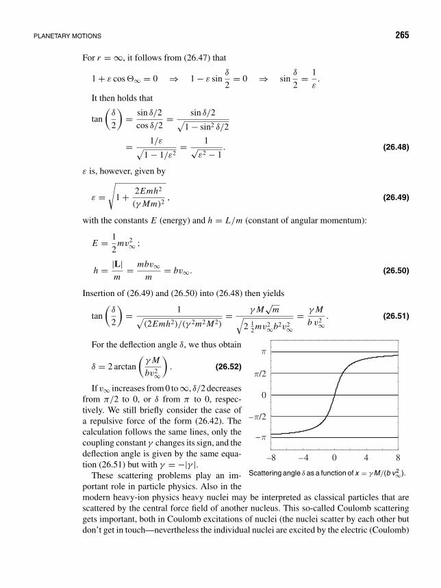
PLANETARY MOTIONS 265
For r = ∞, it follows from (26.47) that
1 + ε cos ∞ = 0 ⇒ 1 − ε sinδ
2= 0 ⇒ sin
δ
2= 1
ε.
It then holds that
tan
(δ
2
)= sin δ/2
cos δ/2= sin δ/2√
1 − sin2 δ/2
= 1/ε√1 − 1/ε2
= 1√ε2 − 1
. (26.48)
ε is, however, given by
ε =√
1 + 2Emh2
(γ Mm)2, (26.49)
with the constants E (energy) and h = L/m (constant of angular momentum):
E = 1
2mv2
∞ ;
h = |L|m
= mbv∞m
= bv∞. (26.50)
Insertion of (26.49) and (26.50) into (26.48) then yields
tan
(δ
2
)= 1√
(2Emh2)/(γ 2m2 M2)= γ M
√m√
2 12 mv2∞b2v2∞
= γ M
b v2∞. (26.51)
–8 –4 0 4 8
–
–
/2
0
/2
Scattering angle δ as a function of x = γ M/(b v2∞).
For the deflection angle δ, we thus obtain
δ = 2 arctan
(γ M
bv2∞
). (26.52)
If v∞ increases from 0 to ∞, δ/2 decreasesfrom π/2 to 0, or δ from π to 0, respec-tively. We still briefly consider the case ofa repulsive force of the form (26.42). Thecalculation follows the same lines, only thecoupling constant γ changes its sign, and thedeflection angle is given by the same equa-tion (26.51) but with γ = −|γ |.
These scattering problems play an im-portant role in particle physics. Also in themodern heavy-ion physics heavy nuclei may be interpreted as classical particles that arescattered by the central force field of another nucleus. This so-called Coulomb scatteringgets important, both in Coulomb excitations of nuclei (the nuclei scatter by each other butdon’t get in touch—nevertheless the individual nuclei are excited by the electric (Coulomb)

266 PLANETARY MOTIONS 26
forces), as well as in peripheral nucleus–nucleus collisions (the nuclear forces hardly play arole in a grazing touch of nuclei—only very few nucleons may be excanged between nuclei).(see, e.g., J.M. Eisenberg and W. Greiner, Nuclear Theory, Vols. 1–3, North Holland,Amsterdam, 1985).
Problem 26.2: Force law of a circular path
A particle moves on a circular path through the origin under the action of a force pointing to the
a x
y
r
θ
Illustration of the orbit and the coordinates used.
origin. Find the force law
F = + f (r)er . (26.53)
Solution 1. (using the energy law):The path equation expressed in plane polar
coordinates reads
r = 2a cos θ. (26.54)
For central forces holds the energy equation (26.19):
E = mh2
2r 4
((dr
dθ
)2
+ r 2
)+ V (r) = constant,
h = L
m.
When differentiating the total energy with respect to r , we get
−2mh2
r 5
((dr
dθ
)2
+ r 2
)+ mh2
2r 4
(d
dr
(dr
dθ
)2
+ 2r
)+ dV
dr= 0. (26.55)
We have
dr
dθ= −2a sin θ,
d
dr
(dr
dθ
)2
= d
dr(4a2 − r 2) = −2r. (26.56)
From F = − grad V , it follows that dV/dr = − f (r). Inserting (26.56) in (26.55) hence yields
f (r) = −2mh2
r 5
(4a2 sin2 θ + 4a2 cos2 θ
) = −8a2mh2
r 5, (26.57)
meaning the force law reads
F = −8a2mh2
r 5er . (26.58)
Solution 2. (using equation (26.22)):We may obtain the force F also by taking into account equation (26.22) because
f (r) = f
(1
u
)= −mu2h2
(d2u
dθ2+ u
), where u = 1
2a cos θ. (26.59)

PLANETARY MOTIONS 267
To get f (r), we first have to form d2u/dθ 2:
du
dθ= 1
2a· sin θ
cos2 θ, (26.60)
d2u
dθ 2= 1
2a· cos3 θ + 2 sin2 θ cos θ
cos4 θ= 1
2a
(1
cos θ+ 2 sin2 θ
cos3 θ
). (26.61)
Inserting 26.61 in 26.59, we obtain
f (r) = −mh2 1
4a2 cos2 θ
(2
2a cos θ+ 2 sin2 θ
2a cos3 θ
)= −mh2 · 2
8a3 cos3 θ
(1 + 1 − cos2 θ
cos2 θ
)= −2mh24a2
r 3· 1
4a2 cos2 θ= −2mh24a2
r 5= −8mh2a2
r 5.
From there it again follows that
F = −8a2mh2
r 5er .
Problem 26.3: Force law of a particle on a spiral orbit
A particle in a central force field with the center at the origin of the coordinate frame moves on aspiral path of the form r = e−θ . What is the force law?
Solution Central forces obey equation (26.22) with F(r) = f (r)er :
f
(1
u
)= −mh2u2
(d2u
dθ2+ u
),
with u = 1/r . Here u = eθ , u = u′′. By insertion we find f (1/u) = −2mh2u3; hence
f (r) = −2mh2
r 3.
Problem 26.4: The lemniscate orbit
Determine the force field that forces a particle to follow the lemniscate path r 2 = 2 a2 cos(2θ).
Solution For central forces again equation (26.22) holds:
f
(1
u
)= −mh2u2
(d2u
dθ2+ u
),
where u = 1/r . The path equation then implies
r = a√
2 cos 2θ, u = 1
a√
2 cos 2θ,
du
dθ= sin 2θ
a√
2(cos 2θ)3/2,
d2u
dθ 2= 1
a√
2
(3 sin2 2θ
(cos 2θ)5/2+ 2√
cos 2θ
)= 1
a√
2
(3
(cos 2θ)5/2− 1√
cos 2θ
).

268 PLANETARY MOTIONS 26
y
x
The lemniscate r2 = 2a2 cos 2θ . For 45 < θ <
135, cos θ is negative, and hence there is no“standing figure 8” part in the lemniscate.
Insertion into the above equation yields
f
(1
u
)= −12mh2a4u7
⇒ f (r) = −12mh2a4
r 7.
This lemniscate path is illustrated in the figure.For the sake of completeness we still remind
ourselves of the definition of a lemniscate: Thelemniscate is a particular Cassini4 curve that isdefined as the set of all points P of a plane forwhich the product of the distances r1 = |P F1|and r2 = |P F2| from two fixed points F1 and F2 have a constant value a2 (see figure),
r1 · r2 = a2.
The distance of the two fixed points is |F1 F2| = 2e. If a = e, the Cassini curve turns by definition
e e
a = 10
76
4
e = 6
The definition of Cassini curves.
into a lemniscate. Let F1 and F2 have the co-ordinates (+e, 0) and (−e, 0) in a Cartesiancoordinate frame. Then r 2
1 = (x −e)2 + y2 andr 2
2 = (x + e)2 + y2 hold. From r1 · r2 = a2 weget after squaring the equation
(x2 + y2) − 2e2(x2 − y2)
= a4 − e4
of the Cassini curve. It is a fourth-order curve.In the special case of the lemniscate, a = e,hence
(x2 + y2) − 2e2(x2 − y2) = 0. (26.62)
When changing to polar coordinates (x = r cos ϕ, y = r sin ϕ), we get
r 2 = e2 cos 2ϕ ±√
e4 cos2 2ϕ + (a4 − e4). (26.63)
The shape of a Cassini curve depends on the ratio of a to e. Again, for the special case of thelemniscate, a = e, we get
r 2 = 2 e2 cos 2ϕ . (26.64)
Problem 26.5: Escape velocity from earth
What must be the initial velocity of a projectile to leave the earth? The air friction is to be neglected!
4Giovanni Domenico Cassini, b. June 8, 1625, Parinaldo—d. Sept. 14(?), 1712, Paris. Cassini was professor ofastronomy in Bologna, at the same time fortress architect and appointed to work on river regulation. From 1667he was director of the observatory in Paris. He mostly published astronomic papers. The Cassini curves weresupposed to replace the Kepler ellipses. However, they were published only in 1740 by his son, Jacques Cassini(1677–1756), in his book Elements d’Astronomie.

PLANETARY MOTIONS 269
Solution The attractive force of earth is F = −γ mM/r 2. At the earth’s surface r = R, there is −F = mg =γ mM/R2, that is, g = γ M/R2.
The equation of motion reads
mr = −γmM
r 2.
With r = dv/dt = (dv/dr)(dr/dt) = v(dv/dr), it follows that
v∫v0
v · dv = −r∫
R
γ M
r 2dr;
hence
1
2(v2 − v2
0) = +γ M
(1
r− 1
R
).
This is nothing else but the energy law, which we could have written down immediately:
1
2mv2 − γ mM/r = 1
2mv2
0 − γ mM
R.
If the missile shall leave earth, that means r → ∞. The minimum initial velocity results if the velocityof the missile arriving at r = ∞ just became equal to zero—v(r → ∞) = 0—and therefore
v20 = 2γ M
R= 2gR, v0 ≈ 11
km
s.
This is called the escape velocity that a body (independent of its mass) must have to leave the earth’sgravitational field.
Problem 26.6: The rocket drive
m
v
∆m
v0
e3
The rocket prob-lem.
A rocket of initial mass m0 per unit time expels the quantity of gas α = m/t >
0 with the constant velocity v0. We look for the equation of motion. The gravi-tational force shall be assumed as constant. That means that the rocket problemshall be considered only near the earth’s surface.
Solution The rocket of mass m(t) moves upward with velocity v(t). Thereby the massm is expelled downward with the constant velocity v0 (relative to the rocket).
To describe the motion of the rocket, we must adopt the Newtonian force lawin its original form
dpdt
= F
because the mass of the rocket is variable. It therefore holds that
dpdt
= mdvdt
+ vdm
dt,
where
v = ve3

270 PLANETARY MOTIONS 26
means the vertical velocity. Within the time interval t , the expelled gases carry off the momentum
p′ = m(v − v0)e3 = α(v − v0)t e3 .
This implies a force on the rocket (recoil force) of the magnitude
F ′ = −p ′
t= −α(v − v0)e3.
In addition, there acts the gravity force −mge3. Hence, the Newtonian force law reads
mdv
dt+ v
dm
dt= −α(v − v0) − mg = −mg − dm
dt(v0 − v).
This balance holds in the inertial system that is tightly fixed to earth. With m = m0 − αt anddm/dt = −α, it follows that
mdv
dte3 = +αv0e3 − mge3.
The term αv0 on the right side represents the recoil force. We further conclude that
v∫0
dv =t∫
0
(αv0
m0 − αt− g
)dt,
v(t) = −gt + v0 ·t∫
0
α/m0 dt
1 − (α/m0) t
= −gt − v0
[ln
(1 − α
m0t
)]t
0
= −gt − v0 ln
(1 − α
m0t
).
Obviously, the rocket velocity depends linearly on the exit velocity v0 of the recoil gases. A furtherintegration yields the altitude h(t) the rocket reached:
h =h∫
0
v dt = −1
2gt2 − v0
t∫0
ln
(1 − α
m0t
)dt.
With the substitution u = 1 − (α/m0) t , du = −(α/m0) dt , we get
v0m0
α
t∫t=0
ln u du = v0m0
α
[u ln u − u
]t
t=0
= v0
αm0
[(1 − α
m0t
)ln
(1 − α
m0t
)−(
1 − α
m0t
)]t
t=0
= v0m0
α
[(1 − α
m0t
)ln
(1 − α
m0t
)+ α
m0t
].

PLANETARY MOTIONS 271
Hence, the altitude of the rocket after time t is
h = −1
2gt2 + v0m0
α
(1 − α
m0t
)ln
(1 − α
m0t
)+ v0t.
To determine the moment T of the burnout, we introduce the mass of the casing m1. We then havem0 = m1 + αT , where αT is the mass of fuel.
T = m0 − m1
α.
At the moment of burnout, the rocket has the velocity
v1 = v(T ) = −gm0 − m1
α− v0 ln
m1
m0= −g
m0 − m1
α+ v0 ln
m0
m1
and the altitude
h1 = h(T ) = −1
2g
(m0 − m1
α
)2
+ v0
[m0 − m1
α+ m1
αln
m1
m0
].
The final velocity depends linearly on the exit velocity v0 of the recoil gases and is proportional tothe logarithm of the ratio of initial to final mass. The further motion of the rocket follows accordingto the energy law:
1
2m · v2
1 = m · g · h2 .
The additional altitude h2 the rocket reaches after burnout is calculated as
h2 = v21
2g.
The total ascension altitude of the rocket is therefore
h = h1 + h2 = h1 + v21
2g,
h = 1
2g
(m0 − m1
α
)2
− 1
2g
(m0 − m1
α
)2
+ v0
(m0 − m1
α
)ln
m1
m0
+ v20
2gln2 m1
m0+ v0
m0 − m1
α+ v0
m1
αln
m1
m0,
=(
lnm1
m0+ 1
)v0
m0 − m1
α+ v0 ln
m1
m0
(v0
2gln
m1
m0+ m1
α
).
Problem 26.7: A two-stage rocket
Establish the equation of motion of a two-stage rocket in the homogeneous gravitational field of earth.
Solution Let T be the burnout time of the first stage. For t ≤ T , the quantities s(t) and v(t) are obtained as inProblem 26.6. The mass at start is
m0 = m1 + αT + αT ′ + m2;m1: casing of first stage, αT fuel of first stage,
m2: casing of second stage, αT ′ fuel of second stage.

272 PLANETARY MOTIONS 26
For t = T , the mass is m ′0 = m2 + αT ′. For t > T (h′(t) and v′(t) have the analogous meaning as in
26.6) we have
h(t) = h′(t − T ) + h(T ) + v(T )(t − T ),
v(t) = v′(t − T ) + v(T ).
Problem 26.8: Condensation of a water droplet
A dust particle of negligible mass being under the influence of gravitation begins to fall at timet = 0 through saturated water vapor. The steam thereby condensates with constant rate λ [gram percentimeter] on the dust particle and forms a water droplet of steadily increasing mass.
(a) Calculate the acceleration of the droplet as a function of its velocity and the traversed path.
(b) Determine the equation of motion of the droplet by integrating the expression for the acceleration.Neglect friction, collisions, etc.
Solution (a) The only external force acting on the droplet is the gravitational force
Fg = mg.
According to Newton’s law,
mg = dm
dtv + m
dv
dtand
dm
dt= dm
dx
dx
dt= λv, (26.65)
because the increase of mass dm/dx = λ shall be a constant. According to equation 26.65, theacceleration is
a = dv
dt= mg − λv2
m, (26.66)
and, because the mass of the dust particle at time t = 0 and position x = 0 is assumed to be negligible,we have m = λx , and for equation 26.66 we get the acceleration
a = g − v2
x. (26.67)
(b) The equation of motion for the dust particle shall now be determined by integration of equation26.67. From 26.67 it follows for x = 0 that
x · d2x
dt2+(
dx
dt
)2
− gx = 0. (26.68)
To solve this nonlinear differential equation, we try the ansatz
x = Atn
and substitute it in equation 26.68. We obtain
(Atn)n(n − 1)Atn−2 + (Antn−1)2 − g Atn = 0,
A2n(n − 1)t2n−2 + A2n2t2n−2 − g Atn = 0. (26.69)
Equation 26.69 is fulfilled for n = 2, that is, if the powers of t are equal. By insertion equation 26.69yields
A(2n2 − n) = g or A = g/6

PLANETARY MOTIONS 273
and therefore as solution for x
x = g
6t2. (26.70)
The proposed ansatz may be verified by inserting this solution into equation 26.68. Differentiationof equation 26.70 yields
v = (g/3)t and a = g/3 ,
that is, the acceleration of the droplet is constant and, independent of x , equal to g/3.
Problem 26.9: Motion of a truck with variable load
M0
v0
λ [kg/sec]
A truck with variable load.
An empty truck of mass M0 moves frictionless with velocityV0 on a stretch of track. At the position x = 0 at time t = 0,the truck is loaded with sand with the load rate λ kg/s (seefigure). Determine the position of the truck as a function oftime.
Solution As no external forces are acting on the truck, the change ofmomentum is
d
dt(mv) = 0 or mv = constant, (26.71)
although both m and v are functions of the time. With the initial conditions at the time t = 0 (m = M0
and v = V0), equation 26.71 becomes
mv = M0V0. (26.72)
Because the truck is being loaded with constant rate, the mass change dm/dt = λ is a constant, andwe have
m = M0 + λt.
Insertion into equation 26.72 yields for the velocity
v = M0V0
M0 + λt. (26.73)
With v = dx/dt, equation 26.73 after separation of the variables yields
dx = M0V0dt
M0 + λt(26.74)
= M0V0
λ
d(M0 + λt)
M0 + λt= M0V0
λ
(dk
k
), (26.75)
where k = M0 + λt , and dt = dm/λ = d(M0 + λt)/λ. Integration of equation 26.74 leads to
x = M0V0
λln k + c (26.76)
= M0V0
λln(M0 + λt) + c. (26.77)

274 PLANETARY MOTIONS 26
0 1 2 3 4
t [ /M0]
0.0
0.5
1.0
1.5
2.0
x[M
0V0/
]
The position of the truck as a function of time.
From the initial conditions x = 0 at timet = 0, the constant c is evaluated as
c = − M0V0
λln(M0), (26.78)
and thus equation 26.76 becomes
x = M0V0
λln
(M0 + λt
M0
). (26.79)
Equation 26.79 is plotted in the opposite fig-ure as a function of the dimensionless quan-tities tλ/M0 and xλ/M0V0. The coordinatex thus increases steadily but logarithmicallywith time.
Example 26.10: The reduced mass
In our treatment of the Kepler problem, we had considered up to now one fixed, massive center ofgravitation (the sun) and small bodies (the planets) orbiting in the field of the immobile central mass.What happens if we consider two bodies of comparable mass that are bound together by gravitation,for instance, two stars in a double-star system?
Solution In a system that consists of two interacting masses m1 and m2 and that is not influenced by exteriorforces, the force F between the masses can depend only on the distance vector r = r1−r2 and possiblyon time derivatives of r. This is due to the assumption of homogeneity of space. The equations of
r
R
r1
m2
m1
r2
The definition of the center of mass.
motions for the two masses thus read
m1r1 = F(r, r, t), (26.80)
m2r2 = −F(r, r, t). (26.81)
According to Newton’s third law meaning“action equals minus reaction,” the force onm2 is opposite equal to the force on m1. Onedefines the position vector of the center of massof the two-body system by
R = m1r1 + m2r2
m1 + m2. (26.82)
With this definition, we can decompose the mo-tion of the two-body system into the motionsof the center of mass R and of the distancevector r.
Adding equations 26.80 and 26.81 shows that the second time derivative of R vanishes, that is, thecenter of mass moves uniformly along a straight line through space:
m1r1 + m2r2 = 0, (26.83)
R = 0 . (26.84)

PLANETARY MOTIONS 275
If one multiplies equation 26.80 by m2/(m1 + m2) and subtracts equation 26.81, multiplied bym1/(m1 + m2), one obtains the important relation
m1m2
m1 + m2r = F(r, r, t) . (26.85)
Thus a clear, physical picture emerges for the motion of the two-body system: The motion of the centerof mass is, according to equation 26.82, uniform along a straight line and completely independent ofthe relative motion of the two masses, which is described by equation 26.85. According to 26.85, therelative motion of the two masses m1 and m2 (on which no extarnal forces are acting) corresponds tothe motion of one single mass, called the reduced mass µ,
µ = m1m2
m1 + m2, (26.86)
in a force field described by F(r, r, t). Thus, the two-body problem has been reduced to an effectiveone-body problem for the reduced mass µ. Upon computation of the relative motion r(t) by integratingequation 26.85, the position vectors of the masses m1 and m2 of the two-body system can be obtained as
r1(t) = R(t) + m1
m1 + m2r(t), (26.87)
r2(t) = R(t) − m2
m1 + m2r(t). (26.88)
r1( )t
r2( )t
m2
m1
S
The motion of two masses m1 and m2 under the influence of their mutual gravitational interaction. Bothmasses move along elliptic orbits whose focal points lie in the center of mass of the two bodies.
Problem 26.11: Path of a comet
A comet moves on a parabolic path in the gravitational field of the sun being at rest. Its orbital planecoincides with the orbital plane (idealized as a circle) of earth. The perihelion distance is a third ofthe radius of the earth’s orbit (RE = 1.49 · 1011 m). What is the time of flight of the comet within theearth’s orbit (a perturbation of the comet path by the planets shall be neglected)?

276 PLANETARY MOTIONS 26
S
Armin
RE
B
Orbit of Comet
Orbit of Earth
The orbit of a comet crossing the orbit of the earthat B.
Solution The comet moves on a parabola, namely E =0, ε = 1, with the path equation
r = k
1 + cos θ, k = L2
γ Mmµ.
We have
L: angular momentum of
reduced mass µ = Mm
M + m,
M : sun mass,
m: comet mass,
γ : gravitational constant.
According to (26.13), the energy law reads
µ
2r 2 + L2
2µr 2+ V (r) = E = 0.
We evaluate this relation at the point A where the term (µ/2)r 2 vanishes because there is no radialkinetic energy (the orbit is symmetric with respect to the straight line through A and S):
L2
2µ(rmin)2= −V (rmin) = γ
Mm
rmin(26.89)
⇒(
L
µ
)= (2γ (M + m)rmin)
1/2 =(
2
3γ (M + m)RE
)1/2
. (26.90)
Let the planet be at the perihelion A at the instant t0. The flight time until leaving the radius RE ofthe earth’s orbit at point B is, according to (26.16),
t − t0 =RE∫
rmin
dr√2µ(−V (r) − L2
2µr2 )
(E = 0) (26.91)
=RE∫
RE /3
dr · r√2µ(γ Mmr − L2
2µ)
=√
µ
2γ M · m
RE∫RE /3
dr · r√r − L2
2µγ Mm
. (26.92)
However, according to 26.89,
L2
2µγ Mm=(
2
3γ (M + m)RE
)1
2µ
1
γ Mm
= 1
3RE = rmin,

PLANETARY MOTIONS 277
and therefore,
t − t0 =√
µ
2γ M · m
RE∫RE /3
dr · r√r − RE/3
; (26.93)
with the substitution x := √r − RE/3, dx = (1/2x) dr , 26.93 may be solved:
t − t0 =√
µ
2γ M · m
( 23 RE )1/2∫
0
2x(x2 + RE/3) dx
x
=√
µ
2γ M · m
[2
3x3 + 2
3RE x
]( 23 RE )1/2
0
= 10
9
√2
3R3/2
E
õ
2γ M · m
= 10
9R3/2
E (3γ (M + m))−1/2 .
For the total residence time of the comet within the earth’s orbit (Ttot = 2(t − t0)), we then obtain
Ttot = 20
9R3/2
E (3γ (M + m))−1/2 . (26.94)
For an “ordinary” comet, the mass m may be neglected against the sun’s mass M (M ≈ 330 000earth masses). Insertion of the values RE = 1.49 · 1011 m, γ M = 1.32 · 1020 m3s−2 yields
Ttot = 74.34 days.
Problem 26.12: Motion in the central field
A mass m moves in the central force field with the potential
U (r) = −α
r(α > 0).
(a) Show that any orbit of finite motion (hence not at infinity) is closed. What happens if an additionalterm of the form β/r 3 is added to U (r)?
(b) Show that the vector (Lenz vector)
V = 1
mα[L × p] + r
r
is a conserved quantity. How may it be interpreted?
Solution (a) Because we are dealing with a central force, we may use the expression (26.17) for the variationof the angle as a function of the radius:
θ =∫
L dr
r 2√
2m(E − U (r)) − L2/r 2.

278 PLANETARY MOTIONS 26
Here L is the angular momentum. A revolution of the mass is characterized by the fact that theradius varies, for example, from rmax over rmin back to rmax. The corresponding variation of the angleis then
θ = 2
rmax∫rmin
L dr
r 2√
2m(E − U (r)) − L2/r 2. (26.95)
We now insert U (r) = −α/r and obtain
θ = 2
rmax∫rmin
L dr
r 2√
2m E + 2mα/r − L2/r 2
= 2
rmax∫rmin
L dr
r 2√−(L/r − mα/L)2 + m2α2/L2 + 2m E
= 2
rmax∫rmin
L dr
Cr 2√
1 − (L/r − mα/L)2/C2,
where we set (m2α2)/L2+2m E = C2. This may be integrated immediately ((arccos x)′ = −1/√
1 − x2)
:
θ = 2 arccos(L/r − mα/L)
C
∣∣∣∣rmax
rmin
. (26.96)
Because the motion shall be finite, the mass moves on a Kepler ellipse
r = k
1 + ε cos θ, with k = L2
mα.
rmin and rmax are then uniquely fixed (for given total energy):
rmin = k
1 + ε, rmax = k
1 − ε, 0 ≤ ε < 1, ε =
√1 + 2E L2
mα2.
Insertion yields
θ = 2 arccos(− mαε
L · C
)− 2 arccos
( mαε
L · C
).
Because
C =√
2m E + m2α2
L2= mα
L
√1 + 2E L2
mα2= mα
Lε,
we obtain
θ = 2([
π + n · 2π]
− n · 2π)
= 2π.
But this just means that the path is closed.If one adds to the potential U (r) an additional term in the form of a small perturbation β/r 3, then
θ = 2π or θ = 2π + δθ ; one then observes rosette orbits (perihelion motion).(b) We show that V = 0. We have
V = 1
mα[L × p ] + r
r,

PLANETARY MOTIONS 279
rmax rmaxrmin
rminAphelion
Aphelion
Perihelion
Perihelion
Kepler ellipse (left) and rosette orbit.
and therefore
V = 1
mαL︸︷︷︸
=0, sinceL=constant
×p + 1
mαL × p + 1
rr − r
r 2r.
Using L = m(r × r) and p = mv = −αr/r 3, we get
V = 1
α(r × r) ×
(− α
r 3r)
+ 1
rr − r
r 2r
= 1
r 3
[r 2r − (r · r) r − (r × r) × r
]= 1
r 3
[r 2r − (r · r)r + (r · r)r − (r · r) r
] = 0.
Here we made use of the relation (a × [b × c]) = (a · c)b − (a · b)c. Hence, it follows that
V = constant (26.97)
ϕr
v
The elliptic orbit.
Both [L × p ] as well as r are within the orbital plane; we nowcalculate the angle ϑ enclosed by the Lenz vector and the radiusvector:
V · r = V · r cos ϑ = 1
mα[L × p ] r + r · r
r(26.98)
= − 1
mαL · [r × p ] + r = r − 1
mαL2
⇒ r = L2/mα
1 − V cos ϑ. (26.99)
This is exactly the path curve of a conical section if V = |V| is identified with the eccentricity ε
and ϑ with (ϕ + π): For an ellipse the Lenz vector points from the focal point to the center, and itsmagnitude equals the eccentricity of the orbit. The figure illustrates this result.
Problem 26.13: Sea water as rocket drive
(For pre-Christmas entertainment)In the near future the sun will cool down so much that no life will be possible any more on earth.
A desperate physicist proposes to drill a hole until reach the hot earth’s interior (T = 4000 K) and

280 PLANETARY MOTIONS 26
then letting the sea water in. The emerging jet of steam shall be utilized as rocket drive to move theearth closer to the sun or—if necessary—to another star. How do you judge that proposal?
Solution The molecules of water vapor of T = 4000 K have the kinetic energy 12 mw2 = 3
2 kT ⇒ velocity ofw ≈ 2.4 km/s (with the Boltzmann constant k = 1.38 · 10−23 kg m2/K s2, m = 2.99 · 10−26 kg). Thespherical surface is A = 4π R2. The water volume is V = A · h, where h is the thickness of the waterlayer (ocean layer) (h = 4 km). As only 75 % of the earth’s surface is covered by water, it follows thatV = 0.75 · 4π R2 · h ≈ 1.5 · 109 km3 = 1, 5 · 1021 kg = mω; the mass of earth is M = 5.6 · 1024 kg,i.e., mw/M ≈ 1/4000. The velocity v of earth caused by expelling the water vapor is given by themomentum conservation as
vM = wmw → v = mw
M· w ≈ 1
4000w ≈ 0.6
m
s.
As compared to the orbital velocity of earth of 30 km/s, the recoil velocity of 0.6 m/s is negligible.Thus, the attempt would be useless—except for a depopulation of earth by an induced super-disaster(no life without water). But the attempt is bound to fail in any case, because the molecules ofwater vapor cannot leave earth at all: w ≈ 2.4 km/s are significantly below the escape velocityv∞ ≈ 11 km/s. The vapor thus cannot be expelled at all by earth. The proposed rocket drive doesnot work, as earth and the water vapor form a closed system.
Example 26.14: Historical remark
One might wonder whether Kepler was denied discovering the force law (gravitational law—seeequation (26.10)). After all, it seemingly follows “so easily” from his own laws. Of course, we cannotand will not accuse Kepler of any lack of brilliance and fantasy. He clearly was a master in empiricalresearch and demonstrated fantasy in far-reaching speculations, sometimes even imaginations: forexample, in his thoughts on the possible number of planets: Like the Pythagoreans, he, too, wasconvinced that God had created the world in number and size according to a definite law of numbers.The explanation is as follows: Kepler was a contemporary of Galileo, who survived him by 12 years.Hence, Kepler knew about Galileo’s mechanics, in particular the central concept of acceleration, thelaws of inertia and throw, by correspondence and hearsay, but probably did not realize their meaningin full. Kepler died in 1630, eight years before the appearance of Galileo’s Discorsi in which hismechanics was outlined in 1638. Even more decisive is the fact that Kepler was not equipped withthe theory of curvilinear motion. The elaboration of this theory was begun by Huygens for circularmotion and was completed by Newton for general paths. Without the concept of acceleration forcurvilinear motions, it is impossible to derive the form (26.8) of the radial acceleration from Kepler’slaws by means of simple mathematical operations.
The Newtonian gravitational mechanics emerging from (26.8, 26.10) and the principle of actionand reaction may be considered as a further development of the throw motion discovered by Galileo.Newton writes on this topic:
“That the planets are kept in their orbits by the central forces may be seen from the motion ofthrown stones (stone-bullets). A (horizontally) thrown stone is deflected from the straight path sincegravity is acting on it, and finally it falls to earth along a curved line. If it is thrown with higher velocityit flies further off, and so it might happen that it finally flies beyond the borders of earth and doesno more fall back. Hence, the stones thrown off with increasing velocity from the top of a mountainwould describe more and more wide parabola bows and finally—at a definite velocity—return to thetop of mountain and by this way move about earth.”

PLANETARY MOTIONS 281
An explanation that convinces by intuition and logical conclusions! The “definite velocity” is todaycalled orbital velocity. Its magnitude has been correctly given by Newton from mv2/R = mg forhorizontal throw as v = √
gR = 7900 m sec−1. For a vertical throw into the universe, the necessaryvelocity (escape velocity) results from the energy law (compare Problem 26.5) as v = √
2gR =11 200 m sec−1. Both results hold without taking into account the friction losses by the air.
The English physicist Hooke (1635–1703), the founder of the law named after him in the theory ofelasticity, also came close to the gravitational law. This is evident from the following of his statements:“I shall develop a world system which in every respect agrees with the known rules of mechanics.This system is founded on three assumptions: 1. All celestial bodies exhibit an attraction (gravityforce) directed towards their center; 2. all bodies that are brought into a straight and uniform motionwill move as long on a straight line, until they are deflected by some force and are forced into acurvilinear path; 3. the attractive forces are the stronger, the closer the body is on which they areacting. I could not yet establish by experiments what the various degrees of attraction are. But it isan idea that will enable the astronomers to determine all motions of the celestial bodies according toone law.”
These remarks show that Newton did not at all create his monumental work Principia out ofnothing: It took, on the contrary, his eminent mental power and bold ideas to summarize all that whatGalileo, Kepler, Huygens, and Hooke had created in the fields of physics, astronomy, and mathematicsin a unified manner, and in particular to realize that the force that lets the planets circulate on theirorbits about the sun is identical with the force that causes the bodies on earth to fall to ground.
Mankind needed one-and-a-half millennia to realize this discovery if one considers that alreadyPlutarch (46–120) in the Moralia (“De facie quae in orbe lunae apparet”) stated that the moon isprevented from falling to earth because of the impetus of its circulation, just as does a body being“swung around” by a sling. It was the ingenious Newton, who realized what the “sling” of the planetsis!
Some more remarks on the versatility and brillance of Hooke: In 1665 he wrote the propheticlines: “I often thought that it should be possible to find an artificial glue-like substance being equalor superior to that excrement from which the silkworms produce their cocoon, and that may bespun to fibers by means of nozzles.” It is the basic idea of the manmade fibers which—though twoand a half centuries later—has revolutionized the textile industry! In the same year he anticipatedthe mechanical theory of heat (hence also the kinetic gas theory) in speculative thought: “That theparticles of all bodies, whatsoever solid they may be, nevertheless are vibrating doesn’t need to myopinion any other proof than the fact that all bodies include a certain amount of heat by themselves,and that an absolutely cold body never has been found yet.”

27 Special Problemsin Central Fields
∆V ´r r– ´
rr´
z
y
x
M
Calculation of the forces of an extendedmass distribution on a point mass M.
The gravitational field of extended bodies
So far only the interactions between pointlike masseshave been considered. Now we shall investigate ex-tended bodies concerning their gravitational action.Because of its linearity, the gravitational field ofan extended body may be composed by superposi-tion of the fields of individual (thought as pointlikein their action) partial bodies. When performing alimit transition with the volumes V ′ of the indi-vidual partial bodies approaching zero, the problemis reduced to an integration. The force acting on amass point M is
F = limmi →0
∑i
(−γ Mmi
|r − r′i |3
(r − r′i )
)= −γ M
∫V
r − r′
|r − r′|3 dm ′.
Depending on the kind of mass distribution the differential dm is replaced by volume,area, or line densities (weight functions) multiplied by the corresponding space elementdV , d F , or ds. In the three-dimensional case, the force is given by
F = −γ M∫
(r′)(r − r′)|r − r′|3 dV ′ ,
and correspondingly the potential energy is
V = limmi →0
∑i
(−γ Mmi
|r − r′i |)
= −γ M∫V
(r′)1
|r − r′| dV ′.
Here (r) = dm/dV is the mass density.
282

THE ATTRACTIVE FORCE OF A SPHERICAL MASS SHELL 283
The attractive force of a spherical mass shell
A spherical shell of negligible thickness with the radius a is uniformly covered by mass(constant area density σ = dm/d f ). What is the force on a point of mass M at the distanceR from the center of the shell?
adϑ
adϑϑ
a sin ϑ
r
R
dFdF
dFII
nM
ψ
T
Calculation of the gravitational force of a spherical shell ona point mass M.
Because the mass is distributedover an area, twofold integrationsuffices. We first decompose thespherical surface into circular rings(see following figure).
The radius of a ring is a sin ϑ ,and the surface of the ring is d f =2πa sin ϑ a dϑ. The result of thefirst integration along the circum-ference may be given immediatelyby exploiting the axial symmetry ofthe mass distribution. To each sec-tion of the circular ring there is asecond one, with the force component dF⊥ (perpendicular to n) being equal but oppositelydirected to the first one. Therefore, only the parallel components −dF‖ = d F cos ψ n areefficient, and the attractive force of the total mass ring is
dF = −γ Mσ d f
r2cos ψ n.
The total force of the spherical shell then follows by integration over all circular rings:
F =∫
d F = −γ Mσ2πa2∫
cos ψ sin ϑ
r2dϑ.
We replace the angles by the distance r via the following geometric relations:(a)
r2 = a2 + R2 − 2a R cos ϑ (cosine law),
and in differential form
2r dr = 2a R sin ϑ dϑ or sin ϑ dϑ = r dr
a R,
and
cos ϑ = a2 + R2 − r2
2a R.
(b)
a2 = R2 + r2 − 2r R cos ψ (cosine law).

284 SPECIAL PROBLEMS IN CENTRAL FIELDS 27
This yields
cos ψ = R2 + r2 − a2
2Rr.
Insertion then yields the force
F = −γ Mσ2πa2∫
R2 + r2 − a2
2Rr3
r dr
a R
= −γ Mσπa
R2
∫ (1 + R2 − a2
r2
)dr.
We first consider the case that the mass point M is outside the sphere (R ≥ a). The desiredtotal attractive force on M is obtained by integration between the limits R − a and R + a:
F = −γ Mσπa
R2
R+a∫R−a
(1 + R2 − a2
r2
)dr
= −γ Mσπa
R2
(r
∣∣∣∣R+a
R−a
− R2 − a2
r
∣∣∣∣R+a
R−a
)= −γ Mm
R2,
where m = 4πa2σ denotes the mass of the spherical shell. Hence: A hollow sphere (oflow thickness) with a uniformly distributed mass is acting on the outer space with respectto its mass attraction so as if its total mass were concentrated at the center. This statementalso holds for homogeneous full spheres (see Problem 27.3) and serves as the base for anycalculations of celestial mechanics.
Now let the mass point M be inside the sphere (R ≤ a). The integration is now performedbetween the limits a − R and a + R:
F = −γ Mσπa
R2
(r
∣∣∣∣a+R
a−R
− R2 − a2
r
∣∣∣∣a+R
a−R
)= 0.
Inside a hollow sphere uniformly covered with mass there is no gravitational force.Because the electric force between two charges q1 and q2 is of a similar structure as thegravitational force, namely
Fe = q1q2
|r1 − r2|2r1 − r2
|r1 − r2| ,
all results obtained here may immediately be transferred to the corresponding electricalcharge distributions. In particular, one sees that a uniformly charged spherical shell doesnot admit fields (forces) in its interior.

THE GRAVITATIONAL POTENTIAL OF A SPHERICAL SHELL COVERED WITH MASS 285
The gravitational potential of a spherical shell covered with mass
Because the potential is a scalar, the potential of a circular ring is
dV = −γ Mσ d f
r,
a M
R
Case 1: Point outsidethe sphere
and the potential of the spherical shell is
V =∫
dV = −γ Mσ2πa2∫
sin ϑ dϑ
r= −γ Mσ2πa
R
∫dr.
We again distinguish the two cases, namely:1. Point outside the sphere (R ≥ a)
The integration limits are then (R − a) . . . (a + R).
V = −2πγσa
RM((R + a) − (R − a)) = −γ M
R4πa2σ = −γ Mm
R.
a M
R
Case 2: Pointinside the sphere
2. Point inside the sphere (R ≤ a)
The integration limits are then (a − R) . . . (a + R).
V = −2πγσaM
R((a + R) − (a − R)) = −4πγσ Ma = −γ Mm
a.
The same result may, of course, also be derived from F(r):R ≥ a:
V (R) = −R∫
∞F · dr = γ Mm
R∫∞
1
r2
rr
dr
= γ Mm
R∫∞
1
r2dr = −γ Mm
R.
R ≤ a: The contribution F · dr vanishes everywhere; therefore, the potential mustbe constant everywhere within the spherical shell. If one requires continuity for R = a(otherwise the forces become infinite), then it follows that
V (R) = −γ Mm
afor R ≤ a.
The forces in a central field point along the radial direction. They are conservative andtherefore in polar coordinates of the form
F(r) = −∇V (r) = − ∂
∂rV (r) er .
The potential in the interior of a spherical shell is constant. As electrostatics is also gov-erned by a 1/r2-force law, one there observes the same phenomenon: In the interior of acharged hollow body, no potential differences (voltages) and hence no forces may occur(Faraday cup).

286 SPECIAL PROBLEMS IN CENTRAL FIELDS 27
ar
V r( )
F r( )
The potential and the force between a point mass and a hollow sphere.
Problem 27.1: Gravitational force of a homogeneous rod
y
m
bϑ
e2
–a a xdM
r x b= 2 2
Calculation of the interaction between a mass pointand a rod.
Find the gravitational force of a homogeneousrod of length 2a and mass M on a particle ofmass m that is positioned at distance b from therod in a plane perpendicular to the rod throughthe rod center.
Solution We have
d F = −γ m d M
r 2
and
cos ϑ = b√x2 + b2
.
d F may be decomposed into force compo-nents parallel and perpendicular to the rod. Thecomponents parallel to the rod mutually compensate each other. Only the force components perpen-dicular to the rod, d F⊥ = d F cos ϑ , are efficient.
d F⊥ = −γ m d M cos ϑ
r 2= −γ mσ dx cos ϑ
x2 + b2= −γ mσ dx b
(x2 + b2)3/2,
F =a∫
x=−a
d F⊥ = −2bγ mσ
a∫0
dx
(x2 + b2)3/2= − 2γ mσa
b√
a2 + b2,
F = − γ Mm
b√
a2 + b2e2 because M = 2aσ.
For b a, a series expansion of the square root yields F ∼ 1/b2, as expected.

THE GRAVITATIONAL POTENTIAL OF A SPHERICAL SHELL COVERED WITH MASS 287
Problem 27.2: Gravitational force of a homogeneous disk
m
ϑ
R r b= 2 2
b
rdr
a
Calculation of the force between a masspoint m and a homogeneous disk.
Let a particle of mass m be on the axis of a disk ofradius a at the distance b from the center of the disk.Find the attractive force between the bodies. The diskis assumed to be homogeneously covered with mass.
Solution The circular disk is decomposed into concentricrings. Only the force components perpendicular tothe disk are efficient; the parallel components com-pensate each other.
d F⊥ = d F cos ϑ = −γ m d M cos ϑ
R2,
cos ϑ = b√r 2 + b2
, R =√
r 2 + b2 ,
d M = σ(2πrdr).
Hence the force between the circular ring and themass is
d F⊥ = −γ mσ2πr dr b
(r 2 + b2)3/2,
and the total attractive force is
F =∫
d F⊥ = −2πγ mσb
a∫0
r dr
(r 2 + b2)3/2.
The integral is solved by substituting u2 = r 2 + b2, r dr = u du,
F = −2πγ mσb
√a2+b2∫b
u du
u3= −2πγσm
(1 − b√
a2 + b2
).
For b a, it follows by expansion of the square root that F = −γ mM/b2 with M = πa2σ , as itmust be.
Problem 27.3: Gravitational potential of a hollow sphere
Show that the gravitational potential of a homogeneous hollow sphere with the outer radius b and theinner radius a has the form
V (R) = −2πγ M ·
⎧⎪⎪⎪⎪⎨⎪⎪⎪⎪⎩2
3(b3 − a3)R−1
b2 − a2
b2 − 2
3
a3
R− 1
3R2
for
⎧⎪⎪⎨⎪⎪⎩R ≥ b,
a ≥ R,
b ≥ R ≥ a.

288 SPECIAL PROBLEMS IN CENTRAL FIELDS 27
a
dm d ´rr´dϑ
ϑ0
b
r
R er
M
Calculation of the potential between a masspoint m and a hollow sphere of homogenousmass density ρ.
Solution We call ϑ : polar angle, ϕ: azimuth (for rotationabout the straight O M). According to the cosinelaw,
r 2 = r ′2 + R2 − 2r ′ R cos ϑ,
2r dr = 2r ′ R sin ϑ dϑ,
or
sin ϑ dϑ = r dr
r ′ R. (27.1)
The potential energy dV due to the mass elementdm of the hollow sphere is dV = −γ M dv /r ,where the volume element is dv = dr ′ · r ′dϑ ·r ′ sin ϑ dϕ. M is the mass of the probe particle atpoint M (see figure). To get the total energy, onehas to integrate over ϕ, ϑ , and r ′.
V (R) = −γ M
b∫a
π∫0
2π∫0
r ′2 sin ϑ dϕ dϑ dr ′
r
= −γ M2π
b∫a
π∫0
r ′2 sin ϑ dϑ dr ′
rwith 27.1
= A
R
b∫a
rmax∫rmin
r ′ dr dr ′ with A = −2πγ M.
We now distinguish three cases:1. R ≥ b: Then rmin = R − r ′, rmax = R + r ′, and we get
V (R) = A
R2
b∫a
r ′2dr ′ = A2
3
b3 − a3
R
(= −γ Mm
R
).
2. R ≤ a: rmin = r ′ − R, rmax = r ′ + R. Thus we obtain
V (R) = A
R2R
b∫a
r ′dr ′ = A(b2 − a2).
3. a ≤ R ≤ b: The point M lies at the outer border of a spherical shell with the radii a and R, andat the same time at the inner border of a spherical shell between R and b. The energy may then becomposed of the contributions according to cases 1 and 2:
V (R) = A
(2
3
R3 − a3
R+ b2 − R2
)= A
(b2 − 2
3
a3
R− 1
3R2
).
The forces are calculated by F = − ∂V∂r er .
1. R ≥ b:
F = −4
3πγM
b3 − a3
R2er = −γ
mM
R2er .

STABILITY OF CIRCULAR ORBITS 289
In this case the force on M is such as if the total mass m of the hollow sphere were united at thecenter.
2. R ≤ a: F = 0. In the interior (empty) space of the hollow sphere, there is no gravitational forceat all.
3. a ≤ R ≤ b:
F = γ M4
3π
(a3
R2− R
)er = −γ M 4
3 π(R3 − a3)
R2er = −γ Mm(R)
R2er ,
where m(R) is the mass of the spherical shell with inner radius a and outer radius R (position of theparticle with mass M). The mass shell beyond R does not contribute to the force on M .
Problem 27.4: A tunnel through the earth
A tunnel for mail transportation is drilled from Frankfurt to Sydney (Australia). Determine the timeneeded for the freely falling air tube casing to cover this distance, assuming the earth is at rest andhas a homogeneous mass distribution. Let the air friction be negligible.
R
M
F
S
Cxr
ϑ
Illustration of the earth with Frank-furt (F ) and Sydney (S) as end-points of a tunnel.
Solution The gravitational force within a homogeneous sphere pointsto the center M and has the magnitude kr (compare Problem27.3). At the surface of the sphere, one has mg = k R; hencek = mg/R. From the figure we read off r = x/ sin ϑ . The com-ponent of the gravitational force along the tunnel is therefore−kr sin ϑ = −(mg/R) x .
Hence, the equation of motion is x + (g/R) x = 0, that is,the air tube casing performs a harmonic vibration between Fand S with the period T = 2π
√R/g.
The time needed between F and S is τ = T/2 = π√
R/g.With R = 6370 km and g = 9.81 m/s2, it follows that τ = 42min. Note that this short time does not depend on the distancebetween F and S.
Stability of circular orbits
In any attractive central force field, the attractive force and the centrifugal force may bebrought into equilibrium, such that circular orbits are always possible. In practice (e.g.,telecommunication satellites on geostationary orbits, particles in accelerators), however, itis moreover important that the circular motion is not destroyed by small elongations. Wetherefore investigate how a central force field must be structured to allow for stable circularorbits. We first consider the field with the particular force law
F(r) = − K
rn

290 SPECIAL PROBLEMS IN CENTRAL FIELDS 27
ρr
Veff
Feff > 0 Feff < 0
The effective potential around a stableorbit.
and look for the powers n for which stable orbitsexist. By adding the centrifugal force we obtain theeffective force
Feff(r) = − K
rn+ mθ2r with θ = L
mr2
= − K
rn+ L2
mr3,
and hence the effective potential
Veff(r) = −r∫
∞Feff dr = − K
(n − 1)rn−1+ L2
2mr2; n = 1.
To get a stable circular orbit with the radius r = ,the effective potential Veff(r) must have a minimumat this position:
⇒ Fcentrifug = Fattr.
Thus, the following conditions shall be fulfilled:
∂Veff
∂r
∣∣∣∣r=
= 0 and∂2Veff
∂r2
∣∣∣∣r=
> 0.
The second condition is essential for the path stability. It ensures that for small displacementsof the orbit a backdriving force occurs, pushing the particle toward the stable radius ,namely Feff > 0 for r < and Feff < 0 for r > .
The two conditions lead us to(a)
∂Veff
∂r
∣∣∣∣r=
= K
n− L2
m3= 0, n−3 = mK
L2,
(b)
∂2Veff
∂r2
∣∣∣∣r=
= − nK
n+1+ 3L2
m4> 0,
which is equivalent to
− nK
n−3+ 3L2
m> 0.
Elimination of yields
(−n + 3)L2
m> 0.
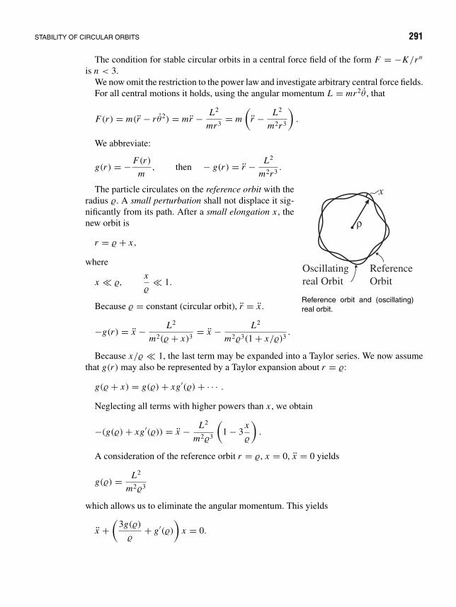
STABILITY OF CIRCULAR ORBITS 291
The condition for stable circular orbits in a central force field of the form F = −K/rn
is n < 3.We now omit the restriction to the power law and investigate arbitrary central force fields.For all central motions it holds, using the angular momentum L = mr2θ , that
F(r) = m(r − r θ2) = mr − L2
mr3= m
(r − L2
m2r3
).
We abbreviate:
g(r) = − F(r)
m, then − g(r) = r − L2
m2r3.
ρ
x
ReferenceOrbit
Oscillatingreal Orbit
Reference orbit and (oscillating)real orbit.
The particle circulates on the reference orbit with theradius . A small perturbation shall not displace it sig-nificantly from its path. After a small elongation x , thenew orbit is
r = + x,
where
x ,x
1.
Because = constant (circular orbit), r = x .
−g(r) = x − L2
m2( + x)3= x − L2
m23(1 + x/)3.
Because x/ 1, the last term may be expanded into a Taylor series. We now assumethat g(r) may also be represented by a Taylor expansion about r = :
g( + x) = g() + xg′() + · · · .
Neglecting all terms with higher powers than x , we obtain
−(g() + xg′()) = x − L2
m23
(1 − 3
x
).
A consideration of the reference orbit r = , x = 0, x = 0 yields
g() = L2
m23
which allows us to eliminate the angular momentum. This yields
x +(
3g()
+ g′()
)x = 0.

292 SPECIAL PROBLEMS IN CENTRAL FIELDS 27
This is just the equation x + ω2x = 0 of the undamped harmonic oscillator with theangular frequency
ω =√
3g()
+ g′().
For ω2 > 0, the solution x = Aeiωt + Be−iωt yields harmonic vibrations. For ω2 < 0 xtends to infinity as Be|ω|t . In the first case the particle “oscillates” on its actual orbit aboutthe reference orbit. In the second case the particle in general runs away from the referenceorbit.
The condition for stable circular orbits thus reads ω2 > 0. For ω2 > 0:
x(t) = Aeiωt + Be−iωt ⇒ x(t) = D sin(ωt + ϕ) (stable);for ω2 < 0 (ω = i |ω|):
x(t) = Ae−|ω|t + Be+|ω|t (unstable).
In the first case the particle vibrates with the small amplitude x about its reference orbit if
3g()
+ g′() > 0,
or3
+ g′()
g()> 0.
Because mg() = −F(), this implies for the force the
stability condition:3
+ F ′()
F()> 0.
When applied to the particular central force field F(r) = −K/rn , the stability conditionimplies
F ′() = nK
n+1; hence
3
− n
n
n+1> 0.
We obtain the condition n < 3, which agrees with our former calculation. This of coursemust be so, since by insertion of Veff one easily realizes that the new stability condition isequivalent to ∂2Veff/∂r2 > 0.
The investigation of path stability may refer, among others, in the atomic range tothe electric field of the nuclei. The simple Coulomb potential V (r) = −K/r allows forstable circular orbits, as was shown already. When taking into account the influence of anoppositely charged electron shell, this potential is weakened: An electron in the outer region“sees” only a small fraction of the nuclear charge. This phenomenon may be taken intoaccount by multiplication by a correction factor < 1. An approximation for the “screenedCoulomb potential” is
V (r) = − K
re−r/a .

STABILITY OF CIRCULAR ORBITS 293
a characterizes the exponential decay of the 1/r -term. Stable circular orbits are also possiblefor the screened potential. One should note that this potential allows for closed orbits evenfor positive energies. The figures illustrate the trend of the potential and the effectivepotential. The closed orbits of positive energy are fully stable in classical mechanics we aretreating here. In quantum mechanics, however, we shall see that these orbits decay, becausethe particles on such orbits of positive energy may “tunnel” through the potential barrier(tunnel effect).
V r( )
V eff
V eff =
r
r
−
−
− +
Kr
Kr
Kr
e−r a/
Lmr
2
22
effectiveCoulomb :Potential
(a)
(b) (c)
Coulomb Potential
screened Coulomb Potential
V eff
V eff =
r
− +Kr
e−r a/ Lmr
2
22
a a= 1
a a= 2
E2
E1
possible closed Orbitwith positive Energy1/ < 1/a a1 2
screened effectivePotentials
Shape of the potential: The screened Coulomb potential (a) decreases rapidly for distances r > a and approacheszero faster than the unsceened potential. Effective Coulomb potential (b) and effective screened Coulomb potential (c).

294 SPECIAL PROBLEMS IN CENTRAL FIELDS 27
Problem 27.5: Stability of a circular orbit
Show that for 2 K > K ′ the circular orbit with r = in the force field F(r) = −K/r 2 − K ′/r 4 isstable (for K , K ′ > 0).
Solution The stability condition reads
3
+ F ′()
F()> 0;
hence
3
+ 2K/3 + 4K ′/5
−K/2 − K ′/4> 0, 32 K + 3K ′ > 22 K + 4K ′, 2 K > K ′.
Problem 27.6: Stability of a circular orbit
Show that a force field with the potential
U (r) = − K
re−r/a with K > 0, a > 0,
allows for stable circular orbits.
Solution F(r) = − ∂
∂rU (r) = −K
(1
ar+ 1
r 2
)e−r/a,
F ′(r) = −K
(− 1
ar 2− 2
r 3
)e−r/a + K
a
(1
ar+ 1
r 2
)e−r/a
= K
(1
a2r+ 2
ar 2+ 2
r 3
)e−r/a .
Insertion into the stability condition yields for r =
3
− 1/a2 + 2/a + 2/2
1/a + 1/> 0.
This means
a2 + a − 2 > 0
or rewritten(
a
)2 −
a− 1 < 0.
This is fulfilled for
a<
1 + √5
2≈ 1.62.

28 The Earth andour Solar System
General notions of astronomy
Stars: Stars are celestial objects (suns) mostly of high mass concentration that emit lightproduced by nuclear reactions. In the core zone of our sun, for example, hydrogen (H)is burning to helium (4He). In other, older stars, higher burning processes are going on,such as 34He → 12C, 12C +4He →16O, etc. They are rather subtle in the details. A clearrepresentation of these processes may be found in J. M. Eisenberg and W. Greiner, NuclearTheory 1: Nuclear Models, 3rd ed., North Holland, Amsterdam (1987).
Planets: Planets are bodies circulating in the central force field of a star. They may reflectlight (the ratio of reflected to incoming luminous flux is called albedo), but hardly emit anylight by themselves (up to some thermal radiation corresponding to their temperatures).The point of maximum distance between a planet and its central body is called aphelion,th point of minimum distance is called perihelion.
Meteors: Collective noun for the light phenomena that are caused by penetration of solidparticles (meteorites) into the earth’s atmosphere. The meteorites that may have massesbetween 10−3 g and 106 kg enter the atmosphere with velocities between 10 and 200 km/sand usually burn out completely.
Comets: Comets are celestial bodies of low mass concentration (most likely all of them)moving in the central force field of a star. A comet has a core out of dust and ice grains.Under sufficient irradiation by the sun it develops a gas shell (coma) and a tail. The totallength may reach up to 300 millions of km.
Satellites: Satellites are bodies circulating about planets. One may distinguish betweennatural satellites, the moons, and artificial ones (the first one was Sputnik I (10/14/1957)).In the case of earth satellites, the longest and shortest distance from earth is denoted as theapogee and perigee, respectively.
295

296 THE EARTH AND OUR SOLAR SYSTEM 28
Asteroids and planetoids: These are pieces of rock. The size is small as compared tothe usual planets. They are orbiting about the sun in the range between Mars and Jupiterand mostly have similar orbital data. Therefore, they were presumed to be the residuesof a decayed planet (the orbits of the planetoids are crossing each other). There are alsocommensurability gaps within the belt of planetoids, presumably caused by Jupiter.
Period: The period denotes the time of a full course of any periodic motion. In astronomyone mostly means the sidereal period, namely, the time a mass needs for a completerevolution about its central body.
Solar system: The sun together with its associated planets and their moons, as well asthe planetoids, comets, and swarms of meteors, in total constitute the solar system.
Ecliptic: The plane in which the center of mass of the system earth–moon orbits aroundthe sun is called ecliptic.
Determination of astronomic quantities
We shall now briefly indicate how astronomic quantities are determined in practice.
The distance between planets and earth
(a) The distances may be determined by triangulation. From a measurement of the obser-vation angles of the planet as seen from two distinct points and of the distance betweenthese points, the distance of the planet may be calculated.
N
S Earth
PlanetParallax
Principal scheme for measuring distances by triangulation.
(b) Distances may be measured by radar. Because the propagation speed of electromagneticwaves is known, one may conclude from the transit time of radar signals on the distance.This method works only for the immediate neighbors of the earth.
(c) In the sense of (a), the earth’s orbit may also be used as a base for triangulation tomeasure the distance of the near fixed stars.

DETERMINATION OF ASTRONOMIC QUANTITIES 297
(d) The sun (and the planets) are moving uniformly by about 610 millions of km/year (or4.09 astronomic units per year) toward the sun’s apex in the constellation of Hercules(see later: “A model of the sun’s environment” and “The spatial motion of the sun” onpage 318 ). This may also be used for parallax measurements, and thus for measuringthe distances of fixed stars up to more than 100 lightyears.
Determination of the distance of far away astronomical objects
The universe is expanding. The farther away the astronomical objects are, the larger theirvelocity is. This extraordinary discovery is due to Edwin Hubble,1 who looked at thelarge-scale behavior of matter in the universe. The Hubble law
v = H0d
allows the determination of the distance d of extragalactic objects from their recessionalvelocity v if the numerical value of the constant H0 is known. Within the theoreticalframework of the Big Bang, the Hubble law is quite plausible. Matter that has beencreated with high initial velocity travels the longest distance within time T : d = vT ; thusv = 1/T · d. For nonrelativistic speeds, the recessional velocity v equals the product of thespeed of light and the redshift z, which can be measured in the spectrum of the observedobject,
z = λ − λ0
λ0.
Here, λ is the observed wavelength of a reference line in the line spectrum of the object andλ0 is the wavelength of this line when the relative velocity between source and observervanishes. If the period of the emitted light is T , we have λ0 = cT and λ = (c + v)T , or
λ0
c= λ
c + v,
from which we obtain v = zc.In order to obtain the Hubble constant H0, the distances of a suitable sample of galaxies
have to be measured. Astronomical distances are usually measured step by step, progressinggradually from the solar system over nearby stars to ever more distant objects, finallyreaching faraway galaxies.2
The first step is the determination of the size of the solar system and of the distances of theplanets. This can be done today very accurately with the help of radar delay measurements.
1Edwin Hubble (1889–1953). American astronomer who determined the extragalactic distance scale by locatingCepheid variables in the galaxy M31 (the Andromeda galaxy) from the Mount Wilson Observatory in 1924 andNGC 6822 in 1925. Extending distance determinations by using the brightest star in galaxies, he proposed theHubble law in 1929.
2For more details about the measurement of astronomical and cosmological distances, see, e.g., Rowan-Robinson, M.: The Cosmological Distance Ladder, W.H. Freeman and Company, 1985.

298 THE EARTH AND OUR SOLAR SYSTEM 28
The only possible way for the direct determination of further distances is the method oftriangulation. This method is suited for the determination of distances of stars in our MilkyWay neighborhood. Here, the change of the direction to a star when observing from twodifferent points at a distance d is measured. The line between the two observation pointsis called the baseline; the angle difference is called the parallax of the star. The parallax isthe same angle under which the baseline would be seen when observed from the star. Thedistance to the star can then be calculated by simple trigonometry. In the ideal (and mostsimple) case, the observed star lies in the plane perpendicular to the baseline and cuts thebaseline in half. Then, the distance is, to a very good approximation, given by
d = b
α,
where b is the length of the baseline and α is the parallax angle. The longest availablebaseline is the line between two opposite points of the earth’s orbit around the sun. This isalso the origin of the distance unit of Parsec (pc). One pc is the distance from which theorbit of the earth is seen under an angle of one arc-second, or, equivalently, the distanceyielding a parallax of one arc-second. 1 Parsec corresponds to 3.26 lightyears.
The range of applicability of the parallax method is given by the error in the determinationof the angle δα and by the restriction in the length of the available baseline. Gaussian errorpropagation yields a relative error for the distance from the parallax method of∣∣∣∣δd
d
∣∣∣∣ =∣∣∣∣ b
α2
∣∣∣∣ δα1
d= δα
d
b.
This means that for a given error in the measurement of the angle α and with a givenbaseline b, not just the absolute error for the distance d, but also the relative error willincrease.
The first parallax of a star was measured by the German astronomer Friedrich WilhelmBessel. In 1838, Bessel published his value of 0.314 arc-seconds for the parallax of thestar 61 Cygni, corresponding to a distance of about 10 lightyears. The correct value of theparallax of 61 Cygni is 0.292 arc-seconds, or 11.2 lightyears.
During the 1990s, the Hipparcos satellite mission measured the parallax of 118,000 starsaccurately down to 1 milliarc-seconds (mas), yielding a very exact picture of the distances inour Milky Way neighborhood.3 But even before the advent of the Hipparcos data, there hadbeen possibilities to measure distances beyond the range of the triangulation method. Withthe help of the star drift parallax (also called convergent-point method) one can measurethe distance to nearby open star clusters and thus determine the absolute luminosity of mainsequence stars.
The method of the star drift parallax is based on the determination of the two componentsof a star’s motion that can be observed from the earth: The radial velocity (the velocityalong the line of sight) can be measured from the Doppler shift in the spectrum of the star,while the proper motion of the star (the motion on the celestial sphere) can be convertedto the transversal velocity if the distance of the star is known. Both velocity componentstaken together yield the compete, three-dimensional velocity vector of the star. If, on the
3See, e.g., Perryman, M.: “The Hipparcos astrometry mission,” Physics Today (June 1998),http://astro.estec.esa.nl/Hipparcos/

DETERMINATION OF ASTRONOMIC QUANTITIES 299
other hand, the direction of the velocity vector and the radial velocity of a star are known,the distance of the star can be calculated from the proper motion. This is used for thedetermination of distances by the star drift parallax method.
If one knows the apparent convergence point of a cluster of stars in collective, parallelmotion, one can deduce the transversal motion of the stars in the cluster from the measure-ment of their radial velocities. By comparison with the proper motion, one can determinethe distance of the stars. The accuracy of this method relies on the large number of measuredstars. The most prominent example for the use of the star drift parallax is the determinationof the distances of the Hyades.4 The distance thus obtained for the Hyades is 45 pc. Thedetermination of the distance to the Hyades serves as a gauge point for methods reachingstill farther out such as the Cepheid method.
When plotting in a diagram the absolute luminosity of stars versus their surface tem-perature, which can be inferred from their spectra, one finds a large class of stars showinga strong monotonic relation between these two observables. Such stars are called mainsequence stars. The diagram is called the Hertzsprung–Russell diagram after its inventors.The fitting of large clusters of stars at the main sequence uses this relation between surfacetemperature and absolute luminosity in order to estimate the absolute luminosity of the starsand, by comparison with the measured apparent luminosities, the distance of the cluster.Thus, the ratio of apparent luminosities of stars in different clusters allows conclusionsabout the ratio of the distances of the clusters to the solar system.
The methods of star drift parallax and fitting to the main sequence thus allow thedetermination of the distance of faraway star clusters. When observing Cepheid stars insuch clusters, one can gauge the period–luminosity relation of this class of variable stars andmeasure distances up to 4 Mpc, reaching beyond the Milky Way in extragalactic regions.
The Cepheid are a class of variable stars that show a definite relation between theirabsolute luminosities (i.e., the total amount of energy released as visible light) and theperiod of variation of their luminosity. They are named after the first known object of thistype, the variable star δ Cephei. When observing a distant Cepheid, measuring the periodof variation thus allows the calculation of the absolute luminosity. Comparing with theapparent luminosity (the light received in a telescope), one can determine the distance ofthe star. In order to obtain reliable results, one must take into account the attenuation of thelight by interstellar matter.
The astrophysical mechanism responsible for the pulsation of Cepheid stars and therelation to absolute luminosity are quite well known. Modern astrophysics differentiatesbetween classical Cepheids and W -Virginis stars, which show different light curves andspectra. Furthermore, one knows the relatively dim R R-Lyrae stars, which can be identifiedfrom their short periods. R R-Lyrae stars have a constant absolute luminosity, which can beused to determine their distance. However, since they are not as bright as Cepheids, theycan be used only over shorter distances.
With the help of extragalactic Cepheids, one can determine the absolute diameter of theH-II regions of galaxies. Assuming that the diameters of large H-II regions of different
4The hyades, an association of several hundred stars, are an open star cluster in the constellation of Taurus (thebull). With a distance of about 145 lightyears, it is the second-closest star cluster to Earth. On the celestial globe,the hyades are centered around Aldebaran, the brightest star in Taurus, which, however, is not part of the hyadescluster.
300 THE EARTH AND OUR SOLAR SYSTEM 28
galaxies are approximately equal, one can then determine the distance to other galaxies.Using this method, one reaches distances up to 25 Mpc.
H-II regions bear their name from the simply ionized hydrogen they consist of. The as-sumption that these regions—which are supposed to play an important role in the formationof stars—are all approximately equal in size relies on the hypothesis that the UV radiationfrom the core of their galaxies which makes them glow always has the same range. Thiswould imply that the observable radius is constant.
The next step uses the distances of the H-II regions in order to determine the absoluteluminosities of so-called Sc-I galaxies. In the Hubble classification of galaxies, Sc-I galaxiesare a class of old spiral galaxies with wide, open spiral arms and a small core. All galaxiesof this class have approximately the same absolute luminosity.
Measuring the apparent luminosity of far away Sc-I galaxies and using their knownabsolute luminosity, one can infer their distance. This finally allows us to determine therelation between distance and redshift and yields a value for the Hubble constant H0.
For every step of the measurement of distances, there also exist alternative methods.Besides the well-established Cepheid calibration, one can look for novae, which havea definite relation between their maximal absolute luminosity and the time scale of thedecrease of luminosity, or for bright main sequence stars, which can be identified from theirspectra and whose absolute luminosity is well known. Supernovae can still be observed inthe huge distance of 400 Mpc. While all supernovae approximately reach the same absoluteluminosity, this value is not easy to calibrate. Still another method uses the third brightestgalaxy in a small galaxy cluster, making the assumption that all such galaxies have nearlythe same absolute luminosity. Experience has shown that the third-brightest galaxy is bettersuited for this purpose than the brightest or second-brightest galaxy. Another possibility forthe determination of distances is the use of the brightest globular clusters of far galaxies.Finally, a radio-astronomical method uses the observed close relation between the half-width of the 21-cm line of hydrogen and the absolute luminosity of a galaxy in the bluespectral band.
The combination of all these different methods yields today a quite coherent picture ofthe distances in the universe. As for the Hubble constant, the accepted value from differentmeasurements by the Hubble space telescope5 is H0 = 72 ± 8 km s−1Mpc−1.
The orbital velocity of the planets
(a) For circular orbits the velocity may be determined from the measurable quantitiesorbital radius and revolution time (period).
(b) For elliptic orbits the velocity may be determined from the measurable quantitiessemi-axes and period.
5Freedman, Wendy L. et al.: “Final Results from the Hubble Space Telescope Key Project to Measure theHubble Constant,” The Astrophysical Journal 553 (2001) 47-72.

DETERMINATION OF ASTRONOMIC QUANTITIES 301
The mass of the planets
(a) From the gravitational law and the equation for the centripetal force the relation γ M =4π2 a3 T −2 follows; see equation (26.41). This is the third Kepler law. M here meansthe mass of the central body, which is large as compared to the mass of the orbitingbody. From this equation one may calculate the mass of the sun and the mass of everyplanet having moons.
(b) If planets don’t have moons, their mass is determined from the orbital perturbations ofthe neighboring planets.
The rotational velocity of a planet or star
The rotational velocity of a planet may be determined by observation of marked pointson its surface. For stars that are visible only as a pointlike light source, this method fails.For these objects the rotational velocity may be derived from their spectra and from thedistortion of a spectral line due to the Doppler effect (distinct shift—red, blue—at oppositesides of the rotating star). The east border of the sun shows, for example, a red shift, andthe west border a blue shift from which follows a rotational velocity of the surface of thesun of 2 km/s.
Detection of gases in the universe
Elements occuring in stars may be determined from the spectrum of the star light. In thecase of planets one has to take into account that they only reflect or absorb light. The gasesof the atmosphere may be identified by the absorption spectrum (Fraunhofer lines).
The tides
Two masses are moving in the gravitational field of a third mass M (see figure).
Ma2 a1
Two masses in the gravitational field of a mass M are subject to different accelerations a1 and a2 dueto the inhomogeneities of the gravitational field.
The first mass is subject to an acceleration a1 = γ M/r21 , the second mass is accelerated
by a2 = γ M/r22 . An observer on one of the masses therefore establishes that the other
mass moves away from it with the acceleration a1 − a2 = γ M(1/r21 − 1/r2
2 ). Hence, thedistinct magnitude of the gravitational force implies a force between the two masses, which

302 THE EARTH AND OUR SOLAR SYSTEM 28
thereby are pulled apart from each other. Such a force always arises if the gravitationalfield is inhomogeneous; it is called a tidal force because the tides on earth are caused bythe same effect.
Low tide and high tide are generated by the motion of the earth in the gravitationalfield of the moon (mass MM). At point A or B (see figure) a body gets an accelerationa = γ MM/(r ± R)2 due to the attractive force of the moon, where r is the distance betweenthe centers of earth and moon, respectively, and R is the earth’s radius.
S
C
MA
DEarth
B
aMaM azazMoon
Explanation of the tides: Earth and moon orbit around the common center of mass S.
The Taylor expansion yields a ≈ (γ MM/r2)(1 ∓ 2R/r). The acceleration at the earth’scenter is az = γ MM/r2, such that the difference is a−az = a−γ MM/r2 = ∓2γ MM R/r3.This difference always points off the earth’s surface and has the magnitude 8 · 10−5 cm/s2.At points A and B the earth’s acceleration is thus reduced by this amount.
The common center of mass S of earth and moon is apart from the earth’s center byabout 3
4 R. Because the center of mass is conserved, both earth and moon are moving withthe same angular velocity about this point S. The center of earth thus moves on a circleof radius 3
4 R about S. This circular motion is the same for all points on earth and leadsto a centrifugal acceleration az that points along the axis earth–moon off the center of thecircle. At the earth’s center the centrifugal acceleration and the gravitational accelerationγ MM/r2 just compensate each other.
The reduction of the earth acceleration at points A and B leads to formation of tidewaves. Because the problem is symmetric about the axis moon–earth, one observes low-tide valleys in the ring through C and D perpendicular to this axis. The points A and B arefloating along the earth’s surface, in accord with the moon’s circulation about earth and therotation of the earth about its axis, such that the highest tide occurs twice within 24 3
4 h at agiven position.
If the earth were completely covered by oceans, the height of the tide wave would amountto about 90 cm. By the various shapes of the coastlines, the times of the highest tide mayshift, and tide waves with heights of several meters may evolve.
The gravitational field of the sun also causes tidal forces on earth that amount to abouthalf of the lunar tidal forces. If sun, moon, and earth lie on a straight line (i.e., at full moonand at new moon, i.e., each 13 1
2 days), the tidal forces add up and a particularly high tidearises (spring tide); at half-moon one observes a neap tide (see figure).

DETERMINATION OF ASTRONOMIC QUANTITIES 303
HalfMoon
New Moon
Full Moon
EarthEarth
Neap TideSpring Tide
Sun
Explanation of spring tide and neap tide.
The friction between the waters andearth implies a deceleration of the earthrotation, such that the day became longerby 0.0165 s during the last 1000 years.Because the total angular momentumof the earth–moon system is conserved,the decrease of the earth’s angular mo-mentum must be joined with an in-crease of the moon’s angular momen-tum. The moon’s angular momentumwith repect to the earth’s center is
Lmoon = MMvr.
The gravitational force just balancesthe centrifugal force:
γ ME MM
r2= MMv2
r⇒ v =
√γ ME
r.
Hence: Lmoon = MM√
γ MEr . If Lmoon increases, the distance earth–moon also increases.This increase amounts to about 3 cm per year.
The transfer of angular momentum from earth to moon is explained in the followingsomewhat simplified model. The friction between the waters of the oceans and the earthcrust causes the two high-tide waves to flow with some delay behind the earth–moon axis(see figure). The differences in the gravitational forces N and F result in a torque thatdecreases the earth’s angular momentum. The sum of the reactive forces acting on themoon has a component along the moon motion. Hence, there exists a torque that increasesthe angular momentum of the moon.
The tidal forces of the earth onto the moon over the ages have resulted in the moon alwaysshowing the same face toward earth: The eigenrotation of the moon is already deceleratedso much that its period coincides with the revolution time of the moon about earth.6
NN
FF
Earth Moon
The high-tide waves are partly convected by the earth rotation.
6We recommend for further reading: Peter Brosche: The deceleration of the earth rotation, Contemporaryphysics (Physik in unserer Zeit) 20 no. 3 (1989) 70.

304 THE EARTH AND OUR SOLAR SYSTEM 28
Precession and nutation of the earth
In the following considerations we always take into account that the celestial bodies (e.g.,earth) have a finite spatial extension.
As the earth has no exact spherical shape but is a flattened rotational ellipsoid, and becausethe rotational axis of the earth is inclined against the ecliptic, the sun performs a torque Donto the earth that generates a change of angular momentum dL of the earth: L = D ordL = D dt . The torque D and hence also dL are perpendicular to the angular momentumL. Because this relation holds at any time, the vector L moves along the surface of a cone,whose axis is the polar axis of the ecliptic. This cone is called the precession cone. Theproblem of motion of spinning bodies will be treated in more detail in connection with thetheory of the top in Classical Mechanics: Systems of Particles and Hamiltonian Dynamics.
Ecliptical Pole
Ecliptical Plane
Earth axis
N
23.4˚
L
S
The geometry of the earth’s precession. The bulge of the geoid is exaggerated.
We consider the problem from the earth’s point of view and base it on the assumptionsthat the sun were circulating about the earth and that the sun’s mass is uniformly distributedalong the assumed path. (This will be justified below.) For our consideration there existsa mass ring about earth at the distance earth–sun. This mass ring generates a change ofangular momentum for the spinning top “earth,” which causes a rotation of the angularmomentum axis about the pole of the ecliptic. In the figure, the pole of the ecliptic standsperpendicular to the assumed (hatched) sun orbit plane, the ecliptic.
The angular momentum axis describes a precession cone about the pole of the ecliptic.The revolution period of the earth precession is 25,730 years (the so-called “platonic year”).This now justifies our assumption of the homogeneous mass ring “sun” since the sun wouldhave performed 25,730 turns about the earth during one period of the precession motion.
Besides the attraction by the sun, still other attractive forces by the moon and otherplanets are acting on earth, which also produce a change of the angular momentum.
The largest perturbations are caused by the moon; they result in precession motions witha period of 9.3 years.

DETERMINATION OF ASTRONOMIC QUANTITIES 305
Because of the flattening of the earth, the earth’s axis and the angular momentum axisdo not coincide exactly, such that the earth’s axis moves about the angular momentumaxis. These fluctuations of the earth’s axis are called nutations. The measured period of thenutation motion of earth is 433 days.
A detailed quantitative discussion of these phenomena is given in the chapter on thetheory of the spinning top (gyroscope) in the volume Classical Mechanics: Systems ofParticles and Hamiltonian Dynamics of these lectures.
Small bodies in the solar system
The more thoroughly the astronomers investigate the solar system, the more difficult itbecomes to maintain the classical subdivision into the various categories for the smallercelestial bodies. Several of the moons orbiting about the planets meanwhile have beenuniquely identified as captured small planets (asteroids). Most of the asteroids, whichpresumably consist of the material of a “prevented” planet, are orbiting about the sunbetween the orbits of Mars and Jupiter. Several of them, however, on their flight alsoclosely approach the earth’s orbit.
It became possible by refined observation techniques to detect even small planets with adiameter of few meters in our neighborhood. Thus, in size they are comparable to meteorites.
At certain time intervals of the year, shooting stars are piling up in the sky, namely alwayswhen the earth is crossing the path of a comet. From that phenomenon the astronomersconclude that many meteorites are fragments of comets. Other meteorites display a com-position that suggests an origin from small planets. It is also known that comets may splitup and decay into debris. Initially intact comets later returned as twin comets.
Such a decay may obviously happen also among small planets. An English–Australianobservation program has led to the discovery of an asteroid in 1991 denoted as 1991 RCand later dubbed “5786 Talos”.7 This object practically follows the same path as the smallplanet Icarus did, which had approached the earth in 1968 to only 6 million km.
In October 1990, the astronomers discovered a small planet with a diameter of only 60 to120 m. One month earlier a telescope on the Kit Peak in Arizona had been set into operationfor a systematic search for small planets in the close vicinity to earth, which raises seriousproblems for the classification of small cosmic objects. By means of this device, a “smallplanet” (1991 BA) of only 5- to 10-m diameter had been detected, which 12 hours laterpassed earth at a distance of 170, 000 km. At tihs time, it was the closest object to earthever detected, and so small that it might also be a meteor.
The systematic search on the Kit Peak for cosmic rocks is performed for the first timeby means of electronic detectors (CCD). Therefore, one has to expect such findings morefrequently in the future. In just October and November 1991, four more objects were foundwith diameters less than 30 m each. Whether these were small planets or meteors could notbe cleared in either case. For a meteor observed in 1972 in the west of the United States,
7D. Steel, Nature 354 265-267 (1991).
306 THE EARTH AND OUR SOLAR SYSTEM 28
it has been estimated that the glowing body had a diameter of 4 m—that is, not much lessthan the object 1991 BA.
By means of the telescope on the Kitt Peak, during only 10 months the astronomers foundevidence for 15 formerly unknown “small planets” on their way toward earth, moreover2000 further asteroids per month. The frequency of collision of such objects with earthwill soon have to be calculated anew with additional data. At a conference held in 1991in St. Petersburg (“The Asteroid Hazard”) the participants still estimated the impact rateof a rock of 50-m diameter to be one event per century. This seems to be a major danger.Actually, meteors so far only rarely have caused noticable damages, because only a verysmall fraction of the earth’s surface is inhabited.
If the object 1991 BA collided with earth, the impact energy—assuming a mass densityof typical meteorite material—would be equivalent to about 40 kilotons of TNT. This isthree times the energy of the Hiroshima bomb. For some time the American space agencyNASA made plans and, indeed, has arranged for systematically localizing small objectsmoving toward earth and, if necessary, to destroy them before a collision. Whether sucha project is meaningful and feasible with present-day means and wether it finds continousfunding remains to be seen.
In this respect it is worthwhile to note that in December 2001, NASA took the decisionto stop a routine search program for small nearby asteroids with the help of the 300-mradio telescope in Arecibo/Puerto Rico. The American Congress had instructed NASA totrack down until 2008 all astronomical bodies larger than 1 km that may represent anydanger to earth. However, Congress did not provide enough funding to accomplish thistask, NASA says. The observations with the telescope in Aceribo are extremely importantfor the determination of the actual position, velocity, and orientation of the orbit of possiblydangerous small objects. Moreover, the telescope allows to take radar maps of some ofthese bodies. The only remaining radio telescope for the search for the “NEOs” (near-earthobjects) is now the antenna of NASA’s Deep Space Network at Goldstone/California. Allother telescopes involved in the search for NEOs are optical telescopes.
Recent research on the solar system—Jupiter’s large family of moons.
The exploration of our solar system is, obviously, far from complete. This view may becorroborated by the discovery of 11 hitherto unknown moons of Jupiter in December 2001,and of further 18 moons during the year 2002, bringing the total number of moons of thelargest planet of our solar system to 58 (as of April 2003).
Jupiter has clearly captured several asteroids and minor planets within its gravitationalfield. The recently discovered moons had been found during a well-directed search programby a group of astronomers from Britain and Hawaii.8 One expects that the overall numberof satellites of Jupiter with a diameter of at least 1 km is well into the hundreds. Furtherdiscoveries will surely be made.
8See, e.g., the web page of the group leader, David Jewitt, from the University of Hawaii, athttp://www.ifa.hawaii.edu/~sheppard/satellites/jup.html.

DETERMINATION OF ASTRONOMIC QUANTITIES 307
This schematic view shows the orbits of the irregular satellites of Jupiter. The outermost regular satellite of Jupiter, theGalilean moon Callisto, is shown for reference. The orbits of the new satellites are shown in black. ( c©University ofHawaii, reproduced with kind permission)
The newly discovered moons all are so-called irregular satellites of Jupiter, characterizedby wide, elliptic orbits that do not lie inside the ecliptic. Many of those irregular satellites(including all the new ones) move along retrograde orbits, namely in a direction oppositeto the direction of Jupiter’s rotation.
The largest one of the irregular satellites, Himalia, was detected already in 1904. Theretrograde orbit of these bodies is a clear hint that they are not primordial satellites ofJupiter, but captured objects. How Jupiter could capture and bind these small planetoids isnot yet known. Astronomers cannot explain these events by celestial mechanics alone. Itmay be possible that Jupiter in the early stages of its history had a far-reaching atmospherethat could slow down the small planetoids.

308 THE EARTH AND OUR SOLAR SYSTEM 28
Jupiter’s new moons all have diameters between 2 and 4 km. They were discoveredwith the help of the Canada–France–Hawaii telescope (diameter 3.6 m) with one of thelargest digital imaging cameras in the world, the “12K”. This camera obtained sensitiveimages of a wide area around Jupiter. The digital images were processed using high-speed computers and then searched with an efficient computer algorithm for objects withmovements characteristic of small moons that are near Jupiter. When the program detectedan object, visual confirmation was made by eye. If the candidate looked good, it wasobserved during succeeding months at the University of Hawaii’s 2.2-m telescope. Theseobservations allowed the computation of their orbits.
Properties, position, and evolution of the solar system
General facts on the solar system
Our solar system belongs to the spiral nebula “Milky Way.” A lateral view of Milky Wayis shown in the following figure. The lines denote zones of equal matter density, with thedensity decreasing from inside to outside. Our solar system is about 10 kpc apart from thecenter of the galaxy. (The length unit parsec has the magnitude 1 pc = 3.086 · 1013 km= 3.26 lightyears. This value stems from the following definition: 1 pc is the distance fromwhere the major radius of the earth’s orbit is seen under 1′′.)
SunSpiral Arms
4 kpc
30 kpc
~~10 light years5 Galactic Halo
Schematic profile of the Milky Way galaxy. The galactic halo is scarcely occupied with old stars, butperhaps filled with so-called dark matter.
Top view of the Milky Way galaxy.
The two figures show how our Milky Way galaxy wouldlook if we could see it from the top or from the side.This “synthetic photography” has been established by acomputer from data measured within our galaxy.
Data on the solar system are compiled in the followingfigures. When considering the solar system, keep in mindthat all planets have the same direction of revolution andalmost the same orbital plane. Only Pluto displays largerdeviations in its data, which led to the assumption that

PROPERTIES, POSITION, AND EVOLUTION OF THE SOLAR SYSTEM 309
Side view of the Milky Way galaxy.
Pluto was captured by the sun only after the evolution ofthe planetary system. In the context of the formation ofthe solar system the following, so far not yet explainedempirical law for the major semi-axes of the planets de-serves interest (the planetoids are well fitting in there). Itis the called the Titius–Bode relation for the major semi-axes an of the planets: an = a0kn .Thereby a0 = 1 AU and k ≈ 1.85. The abbreviation “AU” means “astronomical unit” =major semi-axis of the earth’s orbit. The integer numbers n are associated to the planets(see the figure on p. 309).
MercuryVenus
Mer
cury
Ven
us
EarthMarsPlanetoidsJupiterSaturnUranusNeptunePluto
Ear
th
Mar
s
Cer
es
Jupi
ter
Satu
rn
Ura
nus
Nep
tune
Plut
o
n = 2101234567
−−
0 1 2 3 4 5 6 7 n
− −2 1
lnaa
n
0
Illustration of the Titius–Bode relation.
Sun
Jupiter Saturn
Mer
cury
Ven
usE
arth
Mar
s
Ura
nus
Nep
tune
Plut
o
Illustration of the relative sizes of the planets and the sun.

310 THE EARTH AND OUR SOLAR SYSTEM 28
Our solar system in figures.
Name Sun Mercury Venus Earth MarsCeres
(planetoid)
Symbol —Year of discovery — — — — — 1801
Discoverer — — — — —PiazziGauss
Sidereal period(in earth years)
— 0.205 0.615 1 1.88 4.6
Mean distanceSun–planetin AE
— 0.387 0.723 1 1.524 2.767
Mean distanceSun–planetin 106 km
— 57.9 108.2 149.6 227.9 —
Eccentricityof orbit
— 0.206 0.007 0.017 0.093 0.076
Inclinationof orbit
— 7 3 0 151′ 1037′
Inclinationof equator
— ∼ 2 ∼ 3 2327′ 2359′ —
Radius inearth radii
109 0.382 0.949 1 0.533 0.055
Mass inearth masses
3.3 · 105 0.054 0.814 1 0.107 ∼ 0.0001
Surface gravityin g
— 0.4 0.0.9 1 0.4 —
Density(g/cm3)
1.4 5.46 5.06 5.52 3.93 3.3
Siderealrotation period
∼ 25 d 58d17h −243d 23h56m 24h37m 9h0.5m
Moons — 0 0 1 2 0Mean surface
temperature (in K)5785 100–625 740 288 216 160
Spectroscopicallyfound gasesin atmosphere
H, He He, HCO2, N2,
H2ON2, O2
CO2, N2,O2, H2O
—
Supposed chemicalcomposition(main components)
H, He Fe, SiFe, Si,
OFe, Si,
OFe, Si —

PROPERTIES, POSITION, AND EVOLUTION OF THE SOLAR SYSTEM 311
mEarth = 5.976 · 1024 kg, 1 AE = 1.496 · 106 km.
Name Jupiter Saturn Uranus Neptune Pluto
SymbolYear of discovery — — 1781 1846 1930
Discoverer — — HerschelLeverrier
GalleLowell
TombaughSidereal period
(in earth years)11.8 29.45 84.015 164.78 247.7
Mean distanceSun–planetin AE
5.203 9.539 19.128 30.057 39.50
Mean distanceSun–planetin 106 km
779 1432 2888 4509 5966
Eccentricityof orbit
0.048 0.056 0.047 0.009 0.247
Inclinationof orbit
118′ 229′ 046′ 146′ 1710′
Inclinationof equator
304′ 2644′ 98 29 > 50
Radius inearth radii
10.97 9.03 3.72 3.43 0.24 (?)
Mass inearth masses
317.45 95.21 14.9 17.2 0.002 (?)
Surface gravityin g
2.4 0.9 0.9 1.7 0.1
Density(g/cm3)
1.33 0.71 1.55 2.41 0.8 (?)
Siderealrotation period
9h55m 10h40m −23h50m 17h50m 6h23m
Moons 39 21 5 8 1Mean surface
temperature (in K)134 97 60 57 43 (?)
Spectroscopicallyfound gasesin atmosphere
H2, He,CH4, NH3,
H2O
H2, He,CH4, NH3
H2, CH4H2, He,
CH4, NH3(?)
Supposed chemicalcomposition(main components)
H, He H, HeH2O, CH4,
NH3H, He (?)

312 THE EARTH AND OUR SOLAR SYSTEM 28
Asteroid Belt
Jupiter
MercuryVenusEarthMars
Saturn
Jupiter
Pluto
Neptune
Uranus
1 AU 10 AU
Maps of the solar system in two different scales. 1 AU (astronomical unit) is the radius of the earth’sorbit. The symbol of each planet is given at the perihelion of its orbit.
Closed orbits and perihelion motion
As we have seen, there exist spatially fixed closed orbits in the 1/r -force field. But if thegravitational potential differs somewhat from r−1, hence V (r) = r−1, for example,
V (r) = Ar−1 + Br−2 + Cr−3 + · · · ,a rosette motion may arise. The effective potential has a minimum as before, such that
a minimum and a maximum radius exists. But in general the paths are no longer closedcurves as in the case of the 1/r -potential. They then must be rosette orbits. (We refer toProblem 26.12.)
Deviations from V (r) ∼ r−1, such that the potential differs from cr−1, are caused bythe influence of other planets on the path of a given planet, or by deformation (flattening)of the central star. These perturbations generate both a perihelion motion of the planets
V r( ) ~ V r( ) =1r
1r
rmin
rmax
Closed orbits and rosette orbits in the force field of a central mass.

PROPERTIES, POSITION, AND EVOLUTION OF THE SOLAR SYSTEM 313
as well as the typical rosette path. The planetary orbits agree with the values calculatedaccording to Newton, except for the case where the planet is very close to the sun. Thenormal mutual perturbations of the planets may be calculated by means of the tools ofcelestial mechanics. For Mercury, however, the observed value for the forward motion ofthe Mercury perihelion is too large to be traced back in full to perturbations by other planetsand to the flattening of the sun. The calculated value is by 43′′ per century smaller than themeasured one. Einstein’s theory of general relativity explains this effect.
For the mathematical treatment of the perihelion motion, we refer to Problems 26.12and 28.4.
Evolution of the solar system
A sun is formed if a dense cloud of interstellar gas and dust contracts under the actionof the gravitational force. Our sun is surrounded, however, by many other bodies formingthe planetary system. The evolution of this planetary system is at present not yet fullyunderstood. There are competing theories that always explain only some of the propertiesof the planetary system.
The multitude of theories may be grouped into three main classes that differ in themechanism of formation of the planets.
1. Theories stating that the formation of planets is independent of the formation of the sun:The planets only emerged when the sun was already a normal star. This class includes,for instance, the tidal theories.
2. Theories stating that after the formation of the sun, the planets were generated frominterstellar matter. These are the so-called accretion theories, which assume an increaseof mass within a plane (the ecliptic).
3. Theories according to which the planets are formed out of the same nebula and by asimilar process as the sun is formed (nebular hypotheses).
In the following paragraphs, several of the basic mechanisms of these theories will befurther described.
1. Tidal theories (Bickerton, 1878; Chamberlain, 1901; Moulton, 1905; Jeans, 1916;Jeffreys, 1918)
Two suns pass each other but without mutually capturing each other. Due to the tidalforces, matter is pulled out of the suns that shall condensate to planets. Aside from thelow probability of such an encounter, this theory has several further deficiencies. It couldin no way explain the chemical composition of the planets, and the planet orbits shouldbe strongly elliptic according to this theory. Moreover, some later calculations (Spitzer,1939) showed that matter ejected by a star cannot condense to a planet, because of its hightemperature. Therefore, the tidal theories meanwhile have been dropped.

314 THE EARTH AND OUR SOLAR SYSTEM 28
2. Accretion theories (Hoyle and Littleton, 1939)If the sun moves through a cloud of interstellar matter, it can bind particles by the
gravitational force. Due to the attractive force between the particles and by collisions,larger masses may be formed that shall grow up to the size of the present planets. Onealso has to take into account the consequences of electromagnetic effects (Alfven, 1942).As shown in Example 28.2, the magnetic field of the sun prevents a particle with charge qand mass m to come closer to the sun than to a critical radius rc, which is proportional to(q/m)2/3. Therefore, the heavier particles pile up near the sun. By appropriate assumptionson the magnetic field of the sun, the chemical composition of the planets may be roughlyexplained.
3. Nebular theories (Descartes, 1644; Kant,9 1755; Laplace, 1796)The gas nebula from which the sun originated was flattened by its rotation. Because of
turbulences, parts of the nebula split off, which then begin to contract. They thereby rotatefaster and faster because the angular momentum is conserved. The central part of the nebulaforms the sun, while the peripheral region leads to many proto-planets. In the interior ofthese proto-planets a core evolves from the solid fractions of the nebula. The number ofproto-planets may decrease by collisions.
In more recent time the following mechanism has been investigated: The solid fractions ofthe nebula are enriched in the middle plane of the disk-shaped gas nebula by the gravitationalforce (see figure). With increasing concentration, this dust disk becomes unstable and decaysinto regions of several kilometers of diameter. These regions are the cores for further massaccumulation. Larger and larger objects develop by attraction of further solid particles andby collisions, which grow to the size of planets.
Motion of dust particles in the central plane of a nebula.
9Immanuel Kant, philosopher, b. April 22, 1724, Konigsberg—d. there Feb. 12, 1804.Kant originated from a workman’s family. He attended the pietistic Friedrich gymnasium in his hometown
and until 1746 studied there natural sciences, mathematics, and philosophy; from 1747 to 1754 he was a privatetutor. In 1755 he did his Habilitation in Konigsberg as magister of philosophy; he also served as subordinatelibrarian of the library of the castle. In 1763 he refused an offer for a professorship for poetry; in 1770 he becameprofessor for logic and metaphysics. In 1786 and 1788 he administrated the principalship. In 1796 he stoppedlecturing for health reasons. His life passed without striking external events: He never left East Prussia and rarelyleft Konigsberg [BR].

WORLD VIEWS 315
If a certain size is exceeded, then the gaseous residues of the nebula (H2, He) may bebound by gravitation; hence this theory may also explain the formation of Jupiter andSaturn.
There occurs a temperature gradient within the gas nebula such that the nonevaporatingsubstances (dust particles) are condensing in the hot zone in the interior, while the gases(e.g., H2O, NH3, and CH4) may condense only in the colder zones at larger distance fromthe young sun. This mechanism, in principle, can possibly explain the chemical compositionof the planets.
The angular momentum of our solar system resides to a large extent in the planets. Oursun contains 99.87 % of the mass but only 0.54 % of the total angular momentum available inthe solar system. If the total angular momentum were concentrated to the sun, the resultingvalue would be typical for young stars. Thus one may conclude that the sun must havetransferred angular momentum to the planets. A mechanism for this process is provided bymagneto-hydrodynamics (Hoyle, 1960; Edgeworth, 1962): In the plasma (ionized matter) ofthe gas nebula, very large perturbations may occur, and stabilized magnetic fields, “frozen”in the plasma, may be convected. The transfer of angular momentum from the center to theperipheral region may be explained in this way, similar to the principle of the eddy-currentbrake.
Only in the most recent time have detailed computer simulations of the evolution of agaseous nebula been performed. One must take into account further physical effects (e.g.,pressure, friction, solar wind, tidal forces, etc.). In due time one may judge whether thesetheories actually explain the presently observed properties of the planetary system.
World views
Geocentric—the Ptolemaic world view (about 140 AD)
The Ptolemaic10 world view was the base of astronomy until the 17th century. It considersthe earth as the world center being at rest. The moon, sun and the planets orbit aboutearth. The fact that this world view could survive undisputedly over such a long period isexplained best by a sketch, showing that predictions on the position of the planets couldactually be made, based on this view. It thus had “predictive power.”
If one considers the actual situation (sun in the center of the planetary system), onegets the upper two figures for which hold rp = R + rE or R = rp − rE , respectively.
10Claudius Ptolemy, b. after 83 AD, Ptolemais (middle Egypt)—d. after 161 AD. It is only known that heworked in Alexandria. He is considered as the most important astronomer of the Ancient World. He is themain representative of the geocentric world view. His Great Astronomic System—in the Arabic translationKitab al-magisti known as Almagest—constituted the fundamental work on astronomy until Copernicus. Inhis representation, Ptolemy used the theory of epicycles of the Apollonios, a trigonometry of secants, and thestereographic projection. Ptolemy still published an Optics, the very influential astrologic work Tetrabiblos, andthe most valuable Introduction to Geography, which was extraordinarily influential on science of the MiddleAges, just as astrology.

316 THE EARTH AND OUR SOLAR SYSTEM 28
Sun Sun
Earth
Earth
UpperPlanet
InnerPlanet
R
RrErErp
rp
Inner and outer planets in a heliocentric world model.
Correspondingly, rp circulates about the sun once in one planetary year, and rE does thesame in one earth year. For the geocentric world view, we obtain a different figure:
The equation R = rp −rE also holds in the geocentric world view, but here the Ptolemaicdeferent has been introduced. It is an immaterial circle performed by rp with the sidereanrevolution of the planet about the earth. Because one could not yet determine the distanceof a planet, only the direction of R mattered but not its magnitude. This explains why thetheory of epicycles describes the planetary motion correctly.
Sun Sun
Earth Earth
UpperPlanet
InnerPlanet
RR
rE
rE
rp
rp
Epicycle
Epicycle
Deferent
Deferent
Understanding the theory of epicycles.

WORLD VIEWS 317
2. The heliocentric system—the Copernican world view
In the Copernican world view,11 the sun is understood as the center (central body) of ourplanetary system. It culminated in Kepler’s laws that allowed one to calculate all processesin the planetary system easily and exactly.
11Nicolaus Copernicus, German Koppernigk, Polish Kopernik, astronomer and founder of the heliocentricworld view, named after him Copernican, b. Feb. 19, 1473, Thorn—d. May 24, 1543, Frauenburg (East Prussia).In 1491 he began humanistic, mathematical, and astronomical studies at Cracow University. From 1496–1500he studied civil and clerical law in Bologna. At the instigations of his uncle, Bishop Lucas Watzelrode, he wasadmitted to the chapter of Ermland at Frauenburg in 1497. From autumn 1501 he studied in Padua and Ferrara,graduated there on May 31, 1503, as doctor of canonical law, and then studied medicine. After returning homein 1506, he lived in Heilsberg as secretary of his uncle from 1506 until his uncle’s death in 1512 and wasinvolved in administrating the diocese Ermland. As chancellor of the chapter Copernicus lived from 1512 mostlyin Frauenburg. He resided as governor of the chapter from 1516–1521 in Mehlsack and Allenstein, and in 1523he served as administrator of the diocese of Ermland. From 1522–1529 he represented the order chapter as deputyat the Prussian state parliaments and there in particular also supported a monetary reform.
His paternal family originates from the diocesian country Neiss in Silesia; hence his German origin may beconsidered as established, since in writing he utilized only the German and Latin languages. Copernicus was alsoconsidered as a famous physician, as is indicated by the lily of the valley in one of his woodcuts. As astronomer,Copernicus completed what Regiomontan had imagined: A revision of the doctrine of planetary motion, takinginto account a series of critically evaluated observations. Only on such a basis could one then speculate on acalendar reform. The urgency of this reform was generally recognized at the beginning of the 16th century.Copernicus was presumably influenced by these considerations. In the course of his work he then decided toaccept a heliocentric world system, inspired by vague antique writings. A brief, preliminary report on this topicis the “Commentariolus,” presumably written before 1514. Already here the decisive assumptions are expressed:The sun is in the center of circular planetary orbits, and the earth also circulates about the sun; the earth rotatesdaily about its axis and in turn is orbited by the moon. The wider public got the first information on the Copernicandoctrine by the Narratio Prima of G. J. Rheticus.
The main work of Copernicus, the Six Books on the Orbits of Celestial Bodies (De Revolutionibus OrbiumCoelestium Libri VI, 1543, German 1879, new edition 1939), emerged only in the year Cpernicus died. It wasdedicated to Pope Paul II, but the original foreword of Copernicus was replaced by a foreword of the Protestanttheologist A. Osiander that inverted the meaning of the whole subject. The doctrines of Copernicus remaineduncontested by the Church until the edict of the index congregation of 1616. The remaining imperfections of theCopernican theory of planets were removed by J. Kepler. But just as Copernicus, Kepler could also not prove inmodern sense the correctness of the heliocentric system. Still at the time of I. Newton, the astronomic data werenot precise enough to establish the very small “Copernicus effects.” This was achieved only in 1728 by J. Bradleywith the discovery of the aberration of the fixed stars, and in 1839 by F.W. Bessel by the first measurement of afixed star’s parallax. The objections of the opponents of the Copernican view are intelligible, since for most of thefixed stars the parallaxes are not detectable even by modern methods of measurement, due to the large distancesfrom the sun. His opponents urged, for example, the famous observer T. Brahe to establish his own model of theplanetary system, which represents a compromise between the geocentric and the heliocentric systems [BR].
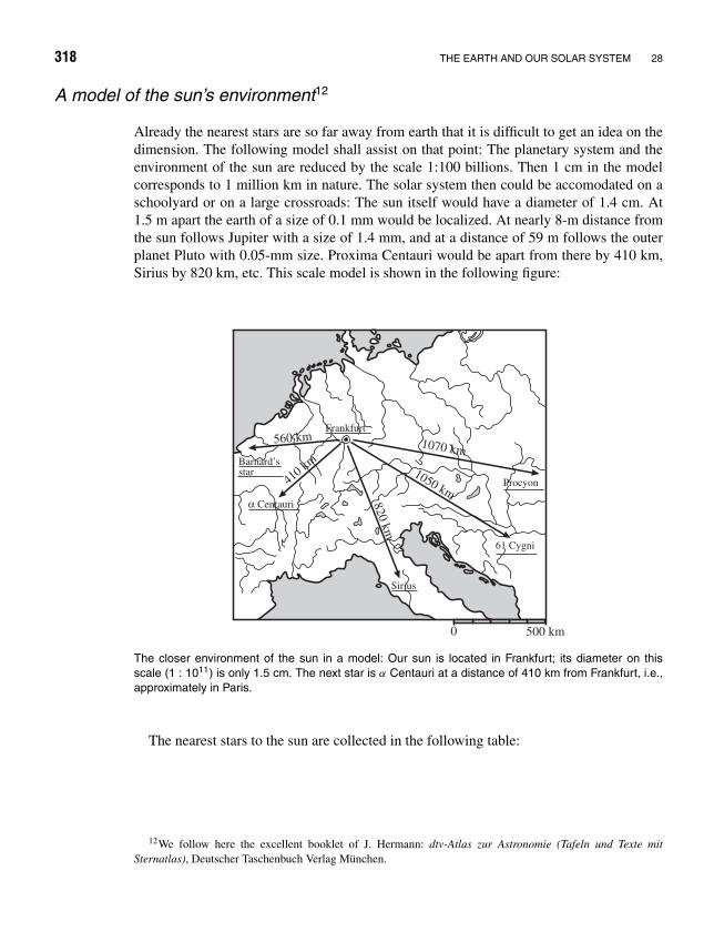
318 THE EARTH AND OUR SOLAR SYSTEM 28
A model of the sun’s environment12
Already the nearest stars are so far away from earth that it is difficult to get an idea on thedimension. The following model shall assist on that point: The planetary system and theenvironment of the sun are reduced by the scale 1:100 billions. Then 1 cm in the modelcorresponds to 1 million km in nature. The solar system then could be accomodated on aschoolyard or on a large crossroads: The sun itself would have a diameter of 1.4 cm. At1.5 m apart the earth of a size of 0.1 mm would be localized. At nearly 8-m distance fromthe sun follows Jupiter with a size of 1.4 mm, and at a distance of 59 m follows the outerplanet Pluto with 0.05-mm size. Proxima Centauri would be apart from there by 410 km,Sirius by 820 km, etc. This scale model is shown in the following figure:
Frankfurt
Procyon
61 Cygni
Sirius
α Centauri
Barnard’sstar
560 km
410 km
820 km
1050 km
1070 km
0 500 km
The closer environment of the sun in a model: Our sun is located in Frankfurt; its diameter on thisscale (1 : 1011) is only 1.5 cm. The next star is α Centauri at a distance of 410 km from Frankfurt, i.e.,approximately in Paris.
The nearest stars to the sun are collected in the following table:
12We follow here the excellent booklet of J. Hermann: dtv-Atlas zur Astronomie (Tafeln und Texte mitSternatlas), Deutscher Taschenbuch Verlag Munchen.

WORLD VIEWS 319
Star Constellation Distance in lightyears
α Centauri/Proxima Centauri Centaurus 4.3Barnard’s arrow star Ophiuchus 5.9Wolf 359 Leo 7.7Luyten 726-8 Cetus 7.9Lalande 21 185 Ursa Maior 8.2Sirius Canis Maior 8.7Ross 154 Sagittarius 9.3Ross 248 Andromeda 10.3ε Eridani Eridanus 10.8Ross 128 Virgo 10.961 Cygni Cygnus 11.1Luyten 789-6 Aquarius 11.2
Other planetary systems?
Due to the large distances between the stars and the fact that planets for themselves arevery dim, there have only recently been successful attempts to obtain strong evidence forthe existence of other planetary systems besides the solar system.13 The star 51 Pegasi (ina distance of about 45 lightyears from the solar system in the constellation of Pegasus)showed periodic variations of its radial velocity (see figure).
This observation can be explained by the motion of the star and an assumed planet aroundtheir common center of mass. The radial motion of the star was deduced from observationsof the Doppler shift of approximately 5000 absorption lines in the spectrum of the star.This methods allows results as precise as 15 m/s. In order to give a better impression of thisvelocity, we mention that the velocity of the sun, which is caused by the common motion ofthe sun and Jupiter is about 13 m/s. The indirectly observed planet, 51 Peg B, is supposedto have roughly the mass of Jupiter (0.5MJ ≤ M ≤ 2MJ) and a nearly circular orbit aroundits solar-type star (ε ≈ 1) with a radius of only 0.05 AU and the short period of T ≈ 2d.This means that when compared to our solar system, the planet would move around clearlywithin the orbit of Mercury. Other possible explanations for the varying radial velocity of51 Pegasi are very improbable.
Current models for the formation of planets do not foresee the emergence of such giantplanets so close to their central stars, leaving the origin of 51 Peg B (and of similar planetsthat have been found since with similar methods) somewhat obscure. Beside the possiblemigration of a giant, Jupiterlike planet to such a close orbit, another explanation may bethe possible capture of a so-called brown dwarf. Brown dwarfs are dim stars whose massis not sufficient in order to ignite the thermonuclear burning of hydrogen in the center of
13M. Major, D. Queloz, “A Jupiter-mass companion to a solar-type star,” Nature 378 (1995) 355; see also, e.g.,Europhysics News 26 (1995) 123.

320 THE EARTH AND OUR SOLAR SYSTEM 28
0
0
51 Peg
Vr (
km s
–1)
m2 sin i = 0.45 MJ
10.5
0.1
–0.1
φThe orbital motion of the star 51 Pegasi, corrected for long-term variations of the velocity of the center ofmass. The points, plotted as a function of the phase of the orbital rotation, correspond to experimentalestimates of the radial velocity as determined from the spectroscopic data. The solid line is the theoreticalcurve fitted for a circular orbit with a period of 4.2293±0.0011 days. It shows that the data are remarkablystable and sinusoidal. (From M. Mayor, D. Queloz, Nature 378 355 (1995) c©Nature Publishing Group,reproduced with kind permission)
the star.14 The periodic variations of the radial velocity of 51 Pegasi show a superimposedperiodic perturbation with a longer period, hinting at a farther planet that is less massive andorbits a greater distance from the star. This implies that one can talk about a real planetarysystem.
Before the discovery of the planet 51 Peg B orbiting a solar-type star, one had alreadyfound two planets with masses comparable to the earth’s mass and periods of severalmonths, orbiting, however, a pulsar.
A further discovery has been the periodic variation of the luminosity of some stars,due to the partial eclipse of the central star by the transit of an orbiting planet15. Thefollowing figure illustrates this method: Data taken with the Hubble space telescope showthe light curve (the luminosity as a function of time) of the solar-type star HD 209458 in theconstellation of Pegeasus. This star has a jupiter-like companion in a very close orbit with
14A good overview and an explanation of the different burning cycles in the interior of a star that is contractingby the gravitational forces can be found in Chapter 18 of J.M. Eisenberg and W. Greiner: Nuclear Theory. Vol 1:Nuclear Models, 3rd ed., North Holland, Amsterdam, 1987.
15L. R. Doyle, H.-J. Deeg, T. M. Brown: Searching for shadows of other Earths, Scientific American, Sep. 2000,p. 38

WORLD VIEWS 321
0.0
1.00
0.99
0.1–0.1Time from center of transit (days)
rela
tive
flux
Left: The light curve of the star HD 209458. The star is partially eclipsed by the transit of its planet. Right: Schematicview of the partial eclipse of HD 209458 by its planet and the resulting light curve. (from T. M. Brown et al., AstrophysicalJournal 552 699-709 (2001), c©American Astronomical Society, reproduced by permission of the AAS.)
a period of about 3.5 days. Every transit of the planet in front of the star yields a dimmingof the star, which is clearly visible in the light curve.
In the meantime (2001), more than 40 planets are believed to exist around stars in thevicinity of our solar system.
The spatial motion of the sun
From the spatial motion of the stars one may conclude that our sun also moves throughthe universe. The method of how to determine this motion is illustrated by the followingexample.
A driver moves by car along a straight road through the woods. If there were no chanceto learn about the direction and speed of motion from other observations, one might deriveit from the motion of the trees. When looking forward along the direction of motion, thetrees seem to diverge. When looking perpendicular to the motion, the trees seem to pass thecar in backward direction. If one looks in backward direction, the trees seem to converge(compare the following figure).

322 THE EARTH AND OUR SOLAR SYSTEM 28
Apex
Antapex
Motional effects that allow the determination of the speed and the direction when driving with constantspeed on a road bordered by trees.
Sun− +Apex Antapex
Radial velocities have the largestnegative value in the direction of theapex, the largest positive value inthe direction of the antapex (dasheddouble arrows). The tangetial veloc-ities of stars are largest in the direc-tion vertical to the sun’s motion (boldarrows), whereas the radial veloci-ties there are smallest.
The same holds also for the motion of the sunthrough the universe: One has to observe the system-atic effects of motion of the stars. A complication ascompared to the case of the moving car, however, isdue to the fact that the stars don’t stand fixed as thetrees, but are moving by themselves. But one may ex-pect that in a statistical observation of very many starsthe individual motions of the other stars will no longershow up too much, such that the effect described abovemanifests itself clearly.
This will of course work only then if the observedstars display no systematic motions, i.e., their individ-ual spatial motions are actually distributed in a purelyrandom manner (statistically). If certain directions ofmotion show up with some preferences, there may arise faults when deriving the spatialmotion of the sun.
This may easily be visualized by assuming, for example, that the trees in the aboveexample move all in one direction, say from left ahead to right behind the car, lookingalong the direction of motion.
Actually the premise of arbitrary directions of motion of the stars is not strictly fulfilled,which makes an exact determination of the sun’s motion rather difficult. Rough assignments,however, could be made already by W. Herschel,16 who at that time investigated only 13
16Sir (since 1816) Friedrich Wilhelm (Willam) Herschel, b. Nov. 15, 1738, Hannover—d. Aug. 25, 1822,Slough near Windsor. At first musician, he went in 1765 as organist to Great Britain. The theory of music led himto mathematics and optics, and in 1766 he began to cut mirrors with such a success that no less than 400 mirrors

WORLD VIEWS 323
stars. Later on the investigations were extended to a much higher number of stars. The sunapex, the target point of the spatial motion of the sun, has the coordinates α = 18 h 04 m,δ = +30, that is, is localized in the constellation of Hercules.
Hercules
Solar Apex
Ras-alhagueRas-algethi
Ophiuchus
Aquila
Lyra
Vega
The position of the sun apex in the constellation of Hercules. Our solar system as a whole—located inthe Orion branch of the Milky Way—moves toward the apex with a speed of 19.4 km/s ≈ 610 millionkm/year.
The velocity of the sun’s motion may be derived from a systematic distribution of theradial velocities of the stars. The stars located in the direction toward the sun apex on theaverage show a negative radial velocity. As a result, one obtains a velocity of 19.4 km/s (610million km/year) for the spatial motion of the sun. This motion relative to the neighboringstars is also denoted as peculiar motion (in contrast to the rotational velocity about thecenter of the Milky Way system).
In 1967 the peculiar motion of the sun could be determined for the first time also byradio-astronomic means, namely by the Doppler shift of the 21-cm radiation of interstellarneutral hydrogen. Taking into account the possible errors of measurement, this result agreeswith the optical observations.
left his workshop. The largest one had a diameter of 1.22 m and 12-m focal length. The observations with hismirrors made him an astronomer. In 1781 he discovered the planet Uranus; in 1783 he established the motion ofthe solar system toward the constellation Hercules; in 1787 he found the two outer moons of Uranus; and in 1789the two inner Saturn moons. His observations of double stars, nebula spots, and stellar clusters opened new fieldsof astronomy, and his star gauges founded the explorations of the structure of the Milky Way system.

324 THE EARTH AND OUR SOLAR SYSTEM 28
Neighbourhood of our Milky Way
Our spiral nebula, the Milky Way, is embedded within the so-called local group, a cluster ofabout 9–10 galaxies. The Milky Way and the Andromeda nebula, just as the M33-galaxy,are spiral nebulas; all other galaxies are of a type of spherical clusters. A widespreadphenomenon in the extended universe is the accumulation of galaxies to galaxy clusters.The first group of galaxies outside the local group is located toward the constellation Virgo;it consists of 2500 galaxies and is at a distance of about 60 million lightyears away.
One should make clear to oneself the ratios of distances: Our Milky Way has a diameterof 105 lightyears; the mean distance of two stars within the Milky Way is about 5 lightyears.The Andromeda nebula is separated from the Milky Way by 2 · 106 lightyears. The MilkyWay is further “orbited” by two small satellite galaxies: The Small and the Large MagellanicCloud.
The famous supernova explosion in the great Magellan cloud was seen on earth onFebruary 24, 1987, the only one in our time whose light curve and neutrino showers have
Draco
SextansUrsa Minor
Sculptor
Fornax
Leo II
Leo I
1.000.000 LY
2.000.000 LY
NGC 6822
IC 1613
M 32
M 33
NGC 147
NGC 185NGC 205
And III
And IAnd II
M 31 (Andromeda Nebula)
Ursa Major
Galaxy (Milky Way)LMC (Large Magellanic Cloud)
SMC (Small Magellanic Cloud)
The local group. Only larger galaxies are shown. The circles indicate the distance from the Milky Way in millions oflightyears.

ON THE EVOLUTION OF THE UNIVERSE 325
been recorded experimentally. Satellite galaxies are frequently observed. Andromeda alsohas two “small” satellite galaxies. The following figure illustrates our neighboring galaxies.
On the evolution of the universe
Our knowledge about the beginning of the universe is rather obscure, because it was bornout of a state which cannot be described by any physical law we know of. We simply callthese indescribable moments of birth of our universe the Big Bang.
Indeed, spectroscopic measurements have shown the existence of a relation betweenthe redshift observed in all star spectra and the distance of the stars from earth. If weassume the Doppler effect as responsible for this shift, then the universe must expand in alldirections. If all motions are now considered in a backward direction, then all bodies meetsimultaneously in a certain space region. Here the cosmic “Big Bang” must have happenedabout 14 · 109 years ago. One imagines that matter (energy) was created by the transitionfrom one state of the vacuum (true vacuum with zero energy) to an energetically deeperstate of vacuum.
After the Big Bang, the universe rapidly expanded from an incredibly small region withdimensions of 10−33 cm and an unthinkably high energy density of 1094 g/cm3—this initialphase of the Universe in known as the Planck aera. The Grand Unified Theories17 of todaysuggest that physics was probably much simpler under the extreme conditions of the Planckaera, because all the forces we nowadays know of—gravitation, electromagnetism, weakinteractions, and strong interactions—were one and the same, or indistinguishable. Theworld was then governed by an universal state of symmetry. However, while the universewas expanding rapidly, this symmetry was quickly broken into present–day forces withvastly different strength and range.
At the extremly short time of 10−23 s after the initial event, the entire now-existingmatter at that time existed in the form of free elementary particles (photons, quarks,gluons, leptons—that is, electrons and neutrinos—, perhaps other, yet unknown elementaryparticles like supersymmetric particles) of enormous concentration (ρ = 1055 g/cm3) andtemperature (T = 1022 K). The expansion and the thereby implied cooling enabled theassembling of nucleons to nuclei, and finally the formation of complete atoms. Under theinfluence of gravitation, the cosmic primordial cloud then condensed to galaxies, and finallyto individual stars.
In the following sections we shall give a short discussion of the modern ideas about theearly universe.18
17see e. g. W. Greiner and B. Muller, Gauge Theories of Weak Interactions, Springer Verlag New York, 200018In this and the subsequent section about dark matter, we follow closely the excellent article by Klaus Pretzl,
In Search of the Dark Matter in the Universe, Spatium 7, May 2000, available from Association Pro ISSI athttp://www.issi.unibe.ch/spatium.html.

326 THE EARTH AND OUR SOLAR SYSTEM 28
The evolution of the universe: Modern physics and experimental observations document the history of the universefrom an incremental fraction of time after the Big Bang some 14 billions of years ago up to its present state. Dark matteris seen today as having played a key role in the formation of stars and galaxies. ( c©CERN Publications, July 1991,reproduced with kind permission)
Inflation and the very early universe.
One observes nowadays enormous homogeneity of the distribution of matter in the universe(averaged over large scales), and also within the Cosmic Microwave Background (CMB)radiation. This is very puzzling because there are regions in the expanding universe whichhave never been in causal contact, that is, light never had sufficient time to travel from oneof these regions to another one.
To overcome this difficulty, some cosmologists (A. Guth, A. Linde, and others) suggestedan exponentially rapid expansion of the universe, blowing up the universe by about a factor3 · 1043 between 10−36 s to 10−34 s after the Big Bang. This expansion is called inflationof the universe. All this reasoning seems utopic, but is helps to understand the present-dayobservations.

ON THE EVOLUTION OF THE UNIVERSE 327
The inflationary phase ended abruptly due to the creation of photons and all the elemen-tary building blocks of matter—quarks and leptons. Equal numbers of matter and antimatterwere present, but most of the energy resided in radiation. The latter lost its energy fasterdue to the expansion, so that after 104 years the energy balance of the universe shifted onfavour of matter.
The hadronic phase transition in the early universe and the CP problem
The quark gluon phase of matter ended about 10−6 seconds after the Big Bang, when theuniverse cooled to a temperature of 2 · 1012 Kelvin. At that temperature a phase transitionfrom a quark gluon plasma to a nucleonic phase of matter took place, where the protonsand neutrons were formed.
In this process three quarks of different flavors (so-called up-quarks and down-quarks)combine together to form a proton (two up-quarks and one down-quark) or a neutron(one up-quark and two down-quarks) and similarly antiprotons (two antiup-quarks and oneantidown-quark) or an antineutron (one antiup-quark and two antidown-quarks).
The gluons were given their name because they provide the glue for holding the quarkstogether in the nucleus. They mediate the strong force by exchange between the forcecenters (color charges) similarly as photons mediate the electromagnetic force betweenelectric charges.
It is worthwhile to mention that in heavy nucleus–nucleus collisions at very high energies,one creates such a quark gluon plasma nowadays in the laboratory, for example, at CERN orat RHIC (Brookhaven). The idea is that in such collisions strong compression (up to 5–10times nuclear density) and high temperatures (∼ 1012 Kelvin) occur in a kind of nuclearshockwaves. Under such conditions, the protons and neutrons in the nuclei melt and setfree quarks and gluons.
After the hadronic phase transition, one would expect to end up with the same numberof nucleons and antinucleons, which annihilate each other after creation, leaving us not achance to exist. Fortunately, this was not the case. The reason that we live in a world ofmatter with no antimatter is believed to be due to a very subtle effect, which treats matterand antimatter in a different way during the phase of creation. This effect, known as CP-violation (charge conjugation and parity violation), was first discovered in an acceleratorexperiment by V. Fitch19 and J. Cronin20 in 1964, for which they got the Nobel Prize in1980, and was used by A. Sakharov21 to explain the matter–antimatter asymmetry in theuniverse.
19Val Logsdon Fitch, American nuclear physicist, b. 1923, Merriman, Nebraska. He received his Ph.D. fromColumbia University in 1954. After working on muons and muonic atoms, he started investigating the propertiesof kaons, where he found in 1964, together with Cronin, the CP violation in the decay of the neutral mesons. Fitchand Cronin shared the 1980 Nobel Prize in physics for this discovery.
20James Watson Cronin, American nuclear physicist, b. 1931, Chicago, Illinois. He received his Ph.D. fromUniversity of Chicago, 1955. His interest in strange particles was stimulated by Gell-Mann, and he worked mostlyon kaons, first in Brookhaven, later in Princeton, joining the group of Fitch.
21Andrei Sakharov, Soviet physicist, b. 1921, Moscow—d. 1989. He was fascinated by fundamental physicsand cosmology, but first he spent two decades designing nuclear weapons. He came to be regarded as the father ofthe Soviet hydrogen bomb. Gradually Sakharov became one of the regime’s most courageous critics, a defender

328 THE EARTH AND OUR SOLAR SYSTEM 28
Primordial nucleosynthesis
After further expansion the universe cooled to a temperature of 109 Kelvin, when protonsand neutrons started to hang on to each other to form the light elements like helium,deuterium, lithium, and beryllium. This phase of nucleosynthesis began a few seconds afterthe Big Bang. The heavier elements were only formed many millions years later, mainlyduring star formation and supernova explosions. After their formation, the light nuclei hadhundreds of thousands of years of time in order to catch electrons and build atoms.
The cosmic background radiation
About 300 thousand years after the Big Bang, radiation had not enough energy leftto interact with matter because the excited states of atoms were appreciably higher thanthe photon energies contained in the cosmic radiation. Therefore, the universe becametransparent for electromagnetic radiation. This radiation from the early universe was firstdiscovered by R. Wilson22 and A. Penzias23 in 1965. They received the Nobel Prize for thisfinding in 1978. Their discovery was made by chance, since they were on a mission fromBell Laboratories to test new microwave receivers to relay telephone calls to earth-orbitingsatellites. No matter in what direction they pointed their antenna, they always measured thesame noise. At first, this was rather disappointing to them. But they happened to learn of thework of the physicist G. Gamow24 and the astronomers R. Dicke25 and P. Peebles,26 thus
of human rights and democracy. His commitment as a “spokesman for the conscience of mankind” was honoredby the Nobel Peace Prize in 1975.
22Robert Woodrow Wilson, b. 1936.23Arno Allan Penzias, b. 1933, Munich, Germany, from where his family could escape to the United States in
1939.24George Gamow, b. 1904, Odessa, Russia—d. 1968. Russian-American physicist who worked out the theory
of alpha decay in terms of tunneling through the nucleus’s potential barrier. Gamow showed that, as a star burnshydrogen, the star heats up. He supported the “Big Bang” theory of Lemaitre. He was also a popularizer of science,publishing many works including Mr. Tompkins in Wonderland (1937) and Thirty Years that Shook Physics (1966).
25Robert Dicke, b. 1916, St. Louis—d. 1997. Dicke received his his Ph.D. in 1941 from the University ofRochester. Dicke is widely known for his leadership in developing experimental tests of gravity physics andof the standard gravitational model for the large-scale evolution of our universe. Working at Princeton, he wasresponsible for the famous 1965 paper that proposed that radiation detected near one centimeter wavelength isleft over from the hot Big Bang start of expansion of the universe. Dicke was building a radio antenna to test histheory when Penzias and Wilson discovered the echo by accident. Some physicists thought that Dicke had beenunfairly excluded from sharing the 1978 Nobel Prize with them.
26Philip James Edwin Peebles, b. 1935, Winnipeg. He graduated from the University of Manitoba in 1958. Hethen went to Princeton University as a graduate student in physics, and he has been there ever since, currentlyas Albert Einstein Professor of Science Emeritus. With Robert Dicke and others he predicted the existence ofthe cosmic background radiation and planned to seek it just before it was found by Penzias and Wilson. He hasinvestigated characteristics of this radiation and how it may be used to constrain models of the universe. He hasled statistical studies of clustering and superclustering of galaxies. He has calculated the universal abundancesof helium and other light elements, demonstrating agreement between Big Bang theory and observation. He has

ON THE EVOLUTION OF THE UNIVERSE 329
Full sky map of the cosmic background radiation as seen by the COBE mission. After subtraction of thedipole anisotropy, which is due to the motion of our solar system within the background radiation (stillvisible at top) and our own galaxy’s emission (center), temperature variation of 0.01% unveils matterdensity fluctuations in the very early universe (bottom). ( c©NASA Goddard Space Flight Center andthe COBE Science Working Group. Reproduced with kind permission.)

330 THE EARTH AND OUR SOLAR SYSTEM 28
realizing that the noise they were measuring was finally not the noise of the receiver, butrather the cooled-down cosmic microwave background radiation (CMB) from the Big Bang.From the frequency spectrum and Planck’s law of black body radiation, the temperature ofthe CMB was derived to be 2.7 Kelvin.27 Regardless of which direction the cosmic radiationwas received from, the temperature came out to be the same everywhere, demonstratingthe enormous homogeneity of the universe. The most accurate CMB measurements comefrom the Cosmic Background Explorer satellite mission (COBE), which was sent into orbitin 1989.28. They found temperature variations only at a level of one part in a hundredthousand.
Presently it cannot yet be predicted whether the course of evolution observed so far willbe inverted and the universe will collapse again. If it would expand more and more expandand evaporate into an infinite vacuum, we would be dealing with an “open universe.” Aperiodic expansion and compression, that is, a “pulsating” universe, is also conceivable.
Dark Matter
Where does dark matter come from?
What about the dark matter? Why dark matter at all? When and how is it created? What isit made of? A partial answer to this question is given to us by the COBE cosmic microwavebackground radiation measurements. They show islands of lower and higher temperaturesappearing on the map of the universe which are due to density fluctuations (see lower partof last figure). They were already present at the time radiation decoupled from matter,300 thousand years after the Big Bang, long before matter was clumping to from galaxiesand clusters of galaxies. We have reasons to believe that these density fluctuations aredue to the dark matter, which was probably created from quantum fluctuations during theinflationary phase of the universe. These tiny fluctuations expanded first through inflationand then retarded their expansion due to gravitational binding forces. They then formedthe gravitational potential wells into which ordinary matter fell to form galaxies and starsbillions of years later. All galaxies and clusters of galaxies seem to be embedded into halosof dark matter.
provided evidence of the existence of large quantities of dark matter in the halos of galaxies, and he continues towork on the origin of galaxies. Peebles was one of the first to resurrect Einstein’s cosmological constant, suggestingit was needed in the 1980s. His books on physical cosmology have had a significant impact in convincing physiciststhat the time has come to study cosmology as a respectable branch of physics.
27For more details, see W. Greiner, L. Neise, H. Stocker, Thermodynamics and Statistical Mechanics, Springer,Berlin, New York, Tokyo, 1994.
28See, e.g., G. Smoot, Wrinkles in Time, New York, 1993, a popular account by the COBE leading scientist,the COBE homepage http://space.gsfc.nasa.gov/astro/cobe/, and Ch. L. Bennett, M. S. Turner, and M. White,“The cosmic Rosetta Stone,” Physics Today, Nov. 1997, for a summary of the scientific results of COBE.

DARK MATTER 331
How much matter is in the universe?
At first this question seems to be highly academic. It is not. The fate of our universe dependson its mass and its expansion velocity.
In the 1920s the famous astronomer Edwin Hubble demonstrated that all galaxies aremoving away from us and from each other—we have already mentioned this in the section on“Evolution of the universe.” His discovery was the foundation stone of modern cosmology,which claims that the universe originated about 15 billion years ago in an unthinkably smallvolume with an unthinkably high-energy density, the so-called Big Bang, and is expandingever since.
However, this expansion is counteracted by the gravitational pull of the matter in theuniverse. Depending on how much matter there is, the expansion will continue forever orcome to a halt, which subsequently could lead to a collapse of the universe ending in a BigCrunch, the opposite of the Big Bang. The matter density needed to bring the expansionof the universe to a halt is called the critical mass density, which today would be roughlythe equivalent of 10 hydrogen atoms per cubic meter. This seems incredibly small, like avacuum, when compared to the density of our earth and planets, but seen on a cosmic scaleit represents a lot of matter.
How can we find out how much matter there is? When estimating the visible matter inthe universe, astronomers look in a very wide and very deep region in space and countthe number of galaxies. Typical galaxies containing hundreds of billions of luminous starshave a brightness proportional to their mass.
0
100
10 20 30Radial distance (kpc)
Orb
ital v
eloc
ity (
km/s
)
NGC 3198
Kepler’s law
The observation of constant orbital velocities of stars around the galactic center (here the spiral galaxyNGC 3198) as a function of the radial distance provides convincing evidence for the presence of anextended halo of dark matter surrounding the galaxy. The expected curve from Kepler’s law if therewere no dark matter is also shown. (From K. Pretzl, Spatium 7, May 2000 c©Association Pro ISSI,reproduced with kind permission)

332 THE EARTH AND OUR SOLAR SYSTEM 28
Thus, by simply counting galaxies over a large volume in space and by assuming thatgalaxies are evenly distributed over the entire universe, one can estimate the total mass theycontribute in form of visible mass to the universe.
However, it turns out to be only 1% of the critical mass of the universe. Therefore, if thevisible matter in the form of stars and galaxies were the only matter in the universe, theuniverse would expand forever. We neglected here the amount of matter in form of planets,because they contribute not more than a few percent of the mass of a star. However, it cameas a surprise when Vera Rubin29 and her team found out in the 1970s that the visible starsare not the only objects making up the mass of the galaxies. They measured the orbitalspeeds of stars around the center of spiral galaxies and found that they move with a constantvelocity independent of their radial distance from the center (see figure). This is in apparentdisagreement with Kepler’s law, which says that the velocity should decrease as the distance
Our galaxy (Milky Way) as seen schematically from a distant point in the galactic plane. Dark matterforms a large halo extending far outside the outer edges of the galaxy. (From K. Pretzl, Spatium 7, May2000 c©Association Pro ISSI, reproduced with kind permission)
29Vera Cooper Rubin, b. 1928, Ph.D. from Georgetown University in 1954, working as an astronomer at theCarnegie Institution of Washington. Most of her work centers about the distribution and motion of galaxies.

DARK MATTER 333
of the star from the galactic center increases, provided that all mass is concentrated at thecenter of the galaxy, which seems to be the case if only the luminous matter is considered.
Indeed, starting from Kepler’s third law,
T 2
a3= 4π2
γ M,
and assuming circular orbits for simplicity, we get
v = 2πa
T=√
γ M
a∼ 1√
a.
This distance-dependence is indicated in the figure at the curve labeled “Kepler’s law”.Now, if Kepler’s law, which describes the orbital motion of the planets in our solar systemvery correctly, is valid everywhere in the universe, then the rotational velocities of the starscan only be explained if the mass of the galaxy is increasing with the radial distance fromits center. This is seen from our formula above, which tells us that v = constant impliesM ∼ a, that is, the mass inside the orbit has to grow proportionally to the radius a of theorbit.
Experimental analysis of the rotational velocities in the Andromeda Galaxy M31 from optical observa-tions (V. Rubin, W. Ford, Astrophysical Journal 159 379-404 (1970)) and radio observations at 21-cmwavelength (M. Roberts, R. Whitehurst, Astrophysical Journal 201 327-346 (1975)). (From K. Pretzl,Spatium 7, May 2000 c©Association Pro ISSI, reproduced with kind permission)
Numerical calculations show that there must be at least an order of magnitude morematter in the galaxies than is visible. From measurements that were repeated on hundreds

334 THE EARTH AND OUR SOLAR SYSTEM 28
of different galaxies, it is conjectured that each galaxy must be embedded in an enormoushalo of dark matter, which reaches out even beyond the visible diameter of the galaxy(see figure). Spiral galaxies are surrounded also by clouds of neutral hydrogen, whichthemselves do not contribute considerably to the mass of the galaxy, but which serve astracers of the orbital motion beyond the optical limits of the galaxies. The hydrogen atomsin the clouds are emitting a characteristic radiation with a wavelength of 21 cm, which isdue to a hyperfine interaction between the electron and the proton in the hydrogen atom andwhich can be detected. The Doppler shift of this characteristic radiation tells the velocitywith which the hydrogen atoms (and thus the matter out there) are moving.
These measurements show that the dark matter halo extends far beyond the opticallimits of the galaxies (see figure). But, how far does it really reach out? Very recentlygravitational lensing observations seem to indicate that the dark matter halo of galaxiesmay have dimensions larger than 10 times the optical diameter. It is quite possible thatthe dark halos have dimensions that are already typical for distances between neighboringgalaxies within galactic clusters.
Determining the mass in the universe
The effect of gravitational lensing is a consequence of Einstein’s general relativity. Becauseradiation consists of photons, every photon with frequency ω carries the energy Ephoton =hω/2π . According to Einstein (see Chapter 33), each mass m carries the energy E = mc2,and, consequently, each photon can be attributed a (dynamical) mass
mphoton = hω
2πc2.
Hence, photons (and therefore radiation) can be deflected by a mass M due to gravitationalforces. This is described in more detail in Problem 33.14 and Example 34.4.
The deflection of light by the sun was first observed in 1919, when the apparent angularshift of stars close to the solar limb was measured during a total solar eclipse. This was thefirst, important proof for the validity of Einstein’s theory, according to which light comingfrom a distant star is bent when grazing a massive object due to the space curvature causedby the gravity of the object (see figure).
It was Fritz Zwicky30 in 1937 who realized that the effect of gravitational lensing wouldprovide the means for the most direct determination of the mass of very large galacticclusters, including dark matter. But it took more than 50 years until his suggestion wasfinally realized and his early determination of the mass of the COMA cluster, in 1933, wasconfirmed. With the Hubble telescope in space and the Very Large Telescopes (VLT) at the
30Fritz Zwicky, (1898–1974). Swiss-American astronomer who was professor of astronomy at Caltech. Hestudied extragalactic supernovae and the distribution of galaxies in Coma Berenices. From his observations of theComa galaxy cluster, he suggested already in 1933 that a large amount of matter in this cluster must be invisiblein order to explain the dynmics of the galaxies in the cluster. In 1937 he was the first to consider gravitationallensing by extragalactic objects.

DARK MATTER 335
Space is curved by gravity. The light rays from a distant star are bent by the gravity field of the sun.Thedistant star therefore appears at a different position. (From K. Pretzl, Spatium 7, May 2000 c©AssociationPro ISSI, reproduced with kind permission)
Southern Observatory in Chile, astronomers now have very powerful tools, which allowthem to explore not only the visible, but also the dark side of the universe with gravitationallensing.
An observer sees a distorted multiple image of a light source in the far background,when the deflecting massive object in the foreground is close to the line of sight. The lightsource appears to be a ring, the so-called Einstein ring, when the object is exactly in theline of sight (see figure). If one knows the distance of the light source and the object tothe observer, one is able to infer the mass of the object from the lensing image. With thismethod it was possible to determine the mass of galactic clusters, which turned out to bemuch larger than the luminous matter. It seems that the gravitational pull of huge amountsof dark matter is preventing individual galaxies from moving away from each other and iskeeping them bound together in large clusters, like, for example, the famous Coma cluster.By adding the total matter (dark and luminous matter) in galaxies and clusters of galaxies,one ends up with a total mass that corresponds to about 30% of the critical mass of theuniverse. With only 1% luminous mass, this would mean that there is 30 times more darkmass in the universe. In addition, the universe would be growing forever, since its totalmass is subcritical to bring the expansion to a halt. But as we will see, this seems not to bethe full story.

336 THE EARTH AND OUR SOLAR SYSTEM 28
Gravitational lensing occurs when the gravity field of a massive celestial object bends the path of lightemitted by a distant source. Einstein predicted the deflection of starlight by the sun (top) and the ringthat would appear if the star and the celestial body were aligned perfectly (center). Lens systems foundto date result from the alignment of extragalactic quasars and galaxies (bottom). (From Edwin L. Turner:“Gravitational Lenses”, Scientific American, July 1988 c©Scientific American, Inc. reproduced with kindpermission.)
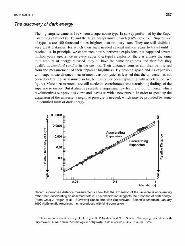
DARK MATTER 337
The discovery of dark energy
The big surprise came in 1998 from a supernovae type 1a survey performed by the SuperCosmology Project (SCP) and the High z-Supernova Search (HZS) groups.31 Supernovaeof type 1a are 100 thousand times brighter than ordinary stars. They are still visible atvery great distances, for which their light needed several million years to travel until itreached us. In principle, we experience now supernovae explosions that happened severalmillion years ago. Since in every supernova type1a explosion there is always the sametotal amount of energy released, they all have the same brightness and therefore theyqualify as standard candles in the cosmos. Their distance from us can then be inferredfrom the measurement of their apparent brightness. By probing space and its expansionwith supernovae distance measurements, astrophysicists learned that the universe has notbeen decelerating, as assumed so far, but has rather been expanding with acceleration (seefigure). More measurements are still needed to corroborate these astonishing findings of thesupernovae survey. But it already presents a surprising new feature of our universe, whichrevolutionizes our previous views and leaves us with a new puzzle. In order to speed up theexpansion of the universe, a negative pressure is needed, which may be provided by someunidentified form of dark energy.
Recent supernovae distance measurements show that the expansion of the universe is acceleratingrather than decelerating as assumed before. This observation suggests the presence of dark energy.(From Craig J. Hogan et al.: "Surveying Space-time with Supernovae", Scientific American, January1999 c©Scientific American, Inc. reproduced with kind permission.)
31For a recent account, see, e.g., C. J. Hogan, R. P. Kirshner and N. B. Suntzef, “Surveying Space-time withSupernovae;” L. M. Krauss, “Cosmological Antigravity,” both in Scientific American, Jan. 1999.

338 THE EARTH AND OUR SOLAR SYSTEM 28
This ubiquitous dark energy amounts to 70% of the critical mass of the universe and hasthe strange feature that its gravitational force does not attract—on the contrary, it repels.This is hard to imagine since our everyday experience and Newton’s law of gravity tell usthat matter is gravitationally attractive. In Einstein’s law of gravity, however, the strengthof gravity depends not only on mass and other forms of energy, but also on pressure. Fromthe Einstein equation, which describes the state of the universe, it follows that gravitationis repulsive if the pressure is sufficiently negative and it is attractive if the pressure ispositive. In order to provide enough negative pressure to counterbalance the attractive forceof gravity, Einstein originally introduced the cosmological constant to keep the universe ina steady state. At that early time all observations seemed to favor a steady-state universewith no evolution and no knowledge about its beginning and its end. When Einstein learnedabout the Hubble expansion of the universe in 1920, he discarded the cosmological constantby admitting that it was his biggest blunder.
For a long time cosmologists assumed the cosmological constant to be negligibly smalland set its value to zero, as it did not seem to be of any importance in describing theevolution of the universe. This has changed very recently, because we know about theaccelerated expansion of the universe. However, there remain burning questions like why isthe cosmological constant so constant over the lifetime of the universe and has not changedsimilar to the matter density, and what fixes its value. Besides the cosmological constant,other forms of dark energy are also discussed by cosmologists, such as vacuum energy,which consists of quantum fluctuations providing negative pressure, or quintessence, anenergy source, that, unlike vacuum energy and the cosmological constant, can vary in spaceand time.
In contrast to dark matter, which is gravitationally attractive, dark energy cannot clump.Therefore, it is the dark matter that is responsible for the structure formation in the universe.Although the true nature of the dark energy and the dark matter is not known, the latter caneventually be directly detected, while the former cannot.
What is the nature of the dark matter?
Baryonic dark matter
The obvious thing is to look for nonluminous or very faint ordinary matter in the form ofplanetary objects like jupiters or brown dwarfs, for example. If these objects represent thedark matter, our galactic halo must be abundantly populated by them.
Because they may not be visible even if searched for with the best telescopes, B. Pac-zynski32 suggested to look for them by observing millions of individual stars in the Largeand the Small Magellanic Cloud to see whether their brightness changes with time due togravitational lensing when a massive dark object is moving through their line of sight (seefigure).
32Bohdan Paczynski, Polish astronomer, b. 1940, Wilno, Poland, now professor of astrophysics, Departmentof Astrophysical Sciences, Princeton University. His main current interest and effort are in the work related to theOptical Gravitational Lensing Experiment.

WHAT IS THE NATURE OF THE DARK MATTER? 339
Massive dark objects (Massive Astrophysical Compact Halo Objects, MACHOs) moving through theline of sight between the observer and a distant star in the Large Magellanic Cloud cause the apparentluminosity to change. (From Bild der Wissenschaft 2/1997, c©bild der wissenschaft)

340 THE EARTH AND OUR SOLAR SYSTEM 28
Several research groups looked for these so-called Massive Astrophysical Compact HaloObjects (MACHOs) using gravitational lensing. They found some of these dark objectswith masses smaller than the solar mass, but by far not enough to explain the dark matterin the halo of our galaxy. Other objects like black holes or neutron stars could also havebeen detected by this method, but there are not many of them in the galactic halo.
Do we know how much ordinary matter exists in the universe? Under ordinary matteror so-called baryonic33 matter, we understand matter in the form of chemical elementsconsisting of protons, neutrons, and electrons. About 3 minutes after the Big Bang, thelight elements, like hydrogen, deuterium, and helium, were produced via nucleosynthesis.From the measurement of their present abundances, one can estimate the total amount ofthe baryonic matter density in the universe. This amounts to not more than 6% of the criticalmass density of the universe. It shows that most of the baryonic matter is invisible and mostof the dark matter must be of nonbaryonic nature.
Nonbaryonic dark matter
The most obvious candidates for nonbaryonic matter would be the neutrinos, if they had amass. Neutrinos come in three flavors. If the heaviest neutrino had a mass of approximately10−9 times the mass of a hydrogen atom, namely mneutrinoc2 = 10−9 · 1GeV = 1eV, itwould qualify to explain the dark matter. This looks like an incredibly small mass, but theneutrinos belong to the most abundant particles in the universe and outnumber the baryonsby a factor of 1010. For a long time it was assumed that neutrinos have no mass. Thestandard model of particle physics34 includes this assumption. All experimental attemptsto determine the mass of the neutrinos ended in providing only upper limits.
However, in 1998 an underground detector with the name SUPER-Kamiokande in Japanobserved anomalies in the atmospheric neutrino flux which is highly suggestive of neutrinooscillations, which can only occur if neutrinos have indeed a mass. These observationswill have to be reproduced and further substantiated by planned accelerator experiments,like K2K in Japan, MINOS in the United States, and OPERA in Europe. The OPERAexperiment will be constructed in the underground Gran Sasso laboratory, which is locatedabout 100 km northeast of Rome. For this experiment, a neutrino beam will be sent fromCERN to the Gran Sasso laboratory. If neutrinos have a mass, they would change theirflavor during their journey over the 735-km distance from CERN to the Gran Sasso. Theneutrinos would start as muon-neutrinos at CERN and would arrive as tau-neutrinos at theGran Sasso. This change of flavor can be detected. Massive neutrinos may also provide thesolution to the puzzle of the missing neutrinos from our sun.
33Barys meaning strong or heavy in ancient Greek.34For more details about neutrinos, see, e.g., W. Greiner, B. Muller, Gauge Theory of Weak Interactions,
Springer Verlag New York, 2000.

WHAT IS THE NATURE OF THE DARK MATTER? 341
A cocktail of nonbaryonic dark matter, neutralinos, and WIMPs
Computer models allow us to study the development of small- and large-scale structuresunder the hypothesis of various nonbaryonic dark matter candidates. Two main categoriesare distinguished, namely the so-called hot and cold dark matter. Neutrinos would qual-ify under the category hot dark matter, since their velocities were very large when theydecoupled from matter, a few milliseconds after the Big Bang. Because of their speedthey were not able to clump on small, typical galactic scales, but their gravitational forcewould still allow for clustering on very large, typical supercluster scales. Thus in a hotdark matter-dominated universe, only the formation of large-scale superclusters would befavored. In such a model superclusters would fragment into smaller clusters at a later time.Hence galaxy formation would be a relatively recent phenomenon, which, however, is incontrast to observation. Cold dark matter candidates, on the other hand, would have smallvelocities at early phases and therefore would be able to aggregate into bound systems at allscales. A cold dark matter-dominated universe would therefore allow for an early formationof galaxies in good agreement with observations, but it would overpopulate the universewith small-scale structures, which does not fit our observations. Questions like how muchhot and how much cold, or only cold dark matter, are still not answered. Some computermodels yield results that come closest to observations when using a cocktail of 30% hotand 70% cold dark matter.
Exotic particles like neutralinos are among the most favored cold dark matter candidates.Neutralinos are stable elementary particles predicted to exist by Super Symmetry (SUSY),a theory that is an extension of the standard model of elementary particles. Thus if theyexist, they would solve two problems at the same time, namely the dark matter as well asSUSY, which is a prerequisite for the unification of all forces in nature, the so-called grandunification theory (GUT). Experiments at the Large Hadron Collider (LHC) at CERN,which is under construction and will be operational in 2005, will also search for theseparticles.
If the dark matter consisted of neutralinos, which would have been produced togetherwith other particles in the early universe and which would have escaped recognition becausethey only weakly interact with ordinary matter, special devices would have to be built fortheir detection. These detectors would have to be able to measure very tiny energies, whichthese particles transfer in elastic scattering processes with the detector material. Becauseof the very weak coupling to ordinary matter, these particles are also called WIMPs, forWeakly Interacting Massive Particles. They would abundantly populate the halo of ourgalaxy and would have a local density in our solar system equivalent to one hydrogen atomin 3 cm3. Because they would be bound to our galaxy, allowing for an average velocityof 270 km/s, their flux (density times velocity) would be very large. However, becausethey only weakly interact with matter, the predicted rates are typically less than one eventper day per kilogram detector material. WIMPs can be detected by measuring the nuclearrecoil energy in the rare events when one of these particles interacts with a nucleus of thedetector material. It is like measuring the speed of a billiard ball sitting on a pool table afterit has been hit by another ball. Because of the background coming from the cosmic raysand the radioactivity of the material surrounding the detector, which yield similar signals

342 THE EARTH AND OUR SOLAR SYSTEM 28
in the detector as the WIMPs, the experiment must be carried out deep underground, wherecosmic rays cannot penetrate, and must be shielded locally against the rest radioactivity ofmaterials and the radioactivity in the rock.
There is presently a race for WIMPs, with several groups in the United States, in Europeand in Japan searching for WIMPs employing different techniques.
Problem 28.1: Mass accretion of the sun
Find the approximate accretion rate d M/dt of the sun if it moves with velocity vs through a homo-geneous gaseous cloud of density .
Solution A particle is captured by the sun if its velocity w in a coordinate frame convected with the sun issmaller than the escape velocity to leave the sun. According to Problem 26.5, the escape velocityreads
v20 = 2γ M
R. (28.1)
For a given constant w all particles will be captured that are localized within a sphere about thesun with the critical radius
R0 = 2γ M
w2. (28.2)
This formula holds, of course, only if R0 exceeds the sun’s radius. To determine the accretion rate,one has to specify how many particles flow into the sphere of radius R0 per unit time.
Let the mean thermal velocity of the gas molecules be vG . We distinguish between two limits:(a) vs vG : In this case the motion of the sun may be neglected, and the mean velocity of the
gas molecules in the coordinate frame fixed to the sun may be set equal to vG .The critical radius according to equation 28.2 is therefore
R0 = 2γ M
v2G
. (28.3)
If the sun were not existent, the numbers of particles flowing into and out of the sphere would bethe same, provided that the velocity vectors vG are distributed isotropically. Not only the moleculesflowing into the sphere will be captured by the sun, but also the particles flying outward will beprevented from escaping and thus will also be captured. Therefore, the mean flow (= particles perunit area per unit time) of captured particles is approximately equal to vG . The accretion rate equalsthe flow multiplied by the surface of the sphere:
d M
dt= 4π R2
0vG = 16πγ 2 M2
v3G
. (28.4)
(b) vs vG : In this case, the thermal motion of the gas molecules may be neglegted. In thecoordinate frame of the sun, all particles then move with the velocity vs . The critical radius is therefore
R0 = 2γ M
v2s
. (28.5)

WHAT IS THE NATURE OF THE DARK MATTER? 343
Because all gas molecules are moving in from the same direction, they “see” only the cross-sectionalarea of this sphere. The accretion rate therefore equals the flow vs multiplied by the area of a circleof radius R0:
d M
dt= π R2
0vs = 4πγ 2 M2
v3s
. (28.6)
Numerical example
We set vs = 0 and thus obtain an upper limit for the accretion rate. For vG we assume a value of103 ms−1 (this corresponds to a temperature of about 100 K for hydrogen molecules). A typical valuefor the density of an interstellar cloud is = 10−18 kg m−3. The sun mass is M = 1.99 · 1030 kg, andthe gravitational constant is γ = 6.67 · 10−11 m3 kg−1 s−2.
According to equation 28.4, it then results that
d M
dt= 8.86 · 1014 kg s−1
= 2.79 · 1022 kg/year
= 4.67 · 10−3 ME /year
with the earth mass ME = 5.975 · 1024 kg.
Example 28.2: Motion of a charged particle in the magnetic field of the sun
If the sun moves through a cloud of interstellar matter, one has to take into account also electromagneticeffects in the calculation of the mass accretion. These shall be estimated below in a simplified model.
The cloud shall contain both gases in ionized form as well as charged solid particles. We considerthe motion of a charged particle of mass m and charge q that moves from far away toward the sun inthe gravitational field and magnetic field of the sun.
For sake of simplicity we assume the magnetic field of the sun as being generated by a dipolewith the magnetic dipole moment µ (for a definition of the dipole moment, see Chapter III in Vol.3: Electrodynamics). Moreover, we shall restrict ourselves to particles moving in the plane passingthrough the center of the sun and being perpendicular to µ.
The Lorentz force acting on the particle in the magnetic field B in this plane is (see volume 3,Electrodynamics):
Fmagn = q
cr × B = q
c
r × µ
r 3, (28.7)
where c is the speed of light.According to (26.10), the gravitational force reads
Fgrav = −γ Mmrr 3
(28.8)
with the sun mass M . Hence, the equation of motion of the particle is
mr = −γ Mmrr 3
+ q
c
1
r 3r × µ.
In plane polar coordinates (r, ϕ) this equation, taking into account (10.11) and (10.12), reads
m((
r − r ϕ2)
er + (r ϕ + 2r ϕ) eϕ
) = −γ Mmer
r 2+ q
c
1
r 3
(rer + r ϕeϕ
)× µ. (28.9)

344 THE EARTH AND OUR SOLAR SYSTEM 28
Because µ is perpendicular to er and eϕ , this equation may be split with respect to the twocomponents:
m(r ϕ + 2r ϕ) = −q
c
µr
r 3(28.10)
mr = −γ Mm
r 2+ q
c
µϕ
r 2+ mr ϕ2. (28.11)
We begin with the first equation. The left side may be transformed such that the following holds:
m
r
d
dt(r 2ϕ) = −q
c
µr
r 3. (28.12)
Integration of this equation yields
mr 2ϕ = −qµ
c
∫r
r 2dt = −qµ
c
∫dr
r 2= qµ
cr+ constant (28.13)
The integration constant may be set to zero if we require the boundary condition that at largedistances from the sun the particle shall have no angular momentum with respect to the sun (the leftside of this equation just represents the angular momentum).
By inserting the result 28.13 in equation 28.11, we obtain
mr = −γ Mm
r 2+ 2q2µ2
mc2r 5. (28.14)
Because
r = dr
dt= dr
drr (28.15)
we get
rdr
dr= −γ M
r 2+ 2q2µ2
m2c2r 5. (28.16)
Integration of this equation yields
r 2 = 2γ M
r− q2µ2
m2c2r 4+ constant (28.17)
With the boundary condition r = 0 for r → ∞, we may set the integration constant to zero. Thereis still another point rc at which the radial velocity vanishes. Solving the equation
2γ M
rc− q2µ2
m2c2r 4c
= 0 (28.18)
yields
rc =(
q2µ2
2γ Mm2c2
)1/3
. (28.19)
Hence, a particle coming from outside can never approach the sun closer than to the radius rc.The only particle parameter entering the formula for rc is the ratio q/m. The interstellar matter
typically contains two kinds of particles: atoms (mainly hydrogen) and solid particles. Solid particleshave a significantly smaller value for q/m than an ionized hydrogen atom and thus may approach thesun much closer than the hydrogen atoms may do.

WHAT IS THE NATURE OF THE DARK MATTER? 345
An estimate of the magnetic field of the sun yields a value of rc of about 1010 km for hydrogen. Theactual value of rc should be somewhat smaller because hydrogen atoms are ionized only at velocitiesof about 5 · 104 ms−1, such that the boundary condition for equation 28.17 must be a distinct one.In any case the minimum distance for hydrogen atoms lies in the external regions of the planetarysystem where the large gas planets are actually localized.
For the solid particles one may assume that only their surface is ionized. One may then estimatetheir q/m-ratio to be proportional to the ratio of surface to volume, that is, inversely proportional totheir radius. The radius of, for example, an interstellar dust particle is typically about 500 times largerthan that of a proton, such that for rc ∼ (q/m)2/3 there should result a value being by about a factorof 100 smaller. This is just the radius of the inner planetary orbits.
Example 28.3: Excursion to the external planets
Many new insights about our solar system have been collected by unmanned space probes such asVoyager I and II. The passage of Saturn by Voyager I (on Nov. 12, 1980) and of Voyager II (on Aug.25, 1981) provided much new knowledge on this planet.35
The Cassini gap of the Saturn rings, caused by the largest moon Titan, is not empty but is alsointerspersed by a number of narrow rings. The Saturn rings consist of countless individual rings, thewidths being about 2 km. Besides the classical 10 Saturn moons, 7 further ones with diameters ofless than 100 km have been detected.
5. Sept. 7720. Aug. 77
Jupiter5. Mar ch 79
Jupiter9. July 79
Saturn12. Nov . 80
Saturn25. Aug. 81
Neptune24. Aug. 89
Uranus24. Jan. 86
PlutoAug. 89
Voyager 2
Voyager 1
Typical pearl string configuration of the exterior planets with the orbits of the Voyager space probesshown. Note the “swing-by” maneuver, i.e., the optimized passages of the planets by the space probesin a kind of “planet swing.”
35The discussion of this problem goes back to suggestions of students of the mechanics course in Frankfurt,using material from various sources.
346 THE EARTH AND OUR SOLAR SYSTEM 28
The newly discovered outer ring, called the F-ring, is slightly eccentric, contrary to the other rings.Moreover, one could detect “spokes” in the Saturn rings. Their origin has not yet been explained,but presumably they may be traced back to a sun flare of the sunlight by tiny ice crystals. Afterabout 4 · 104 years Voyager I will reach the vicinity of the star AC + 793 888 in the constellationUrsa Minor. Voyager II, after an encounter with Neptune on August 24, 1989, will travel a long waythrough innterstellar space, and after 3.58 · 105 years will pass Sirius, the main star of Canis Maiorand the brightest fixed star of the firmament, at a distance of 0.8 lightyears. A difficulty in exploringthe outer planets are the long flight times. These may, however, be shortened significantly if theprobe exploits the gravitational field of a planet on its route for a calculated change of flight direction(swing-by). A rare constellation of the four largest planets Jupiter, Saturn, Neptune and Uranus that isparticularly suited for this purpose arose in the 1980’s: The planets didn’t stand in a straight line butnevertheless along a flat curve. Such a “pearl string configuration” occurs only once in 175 years andallows Voyager II to pass our four largest planets. Due to the increase of kinetic energy by the variouspassages of planets (“swing-bys”), as is seen from the preceding figure, the program of Voyager IImay be finished already after 12 years, while a direct flight with equivalent energy expense wouldlast about 30 years.
The essential aspects of the calculated trajectories with gravitational support for such a missionmay already be elaborated from the equations on planetary motion in Chapter 26.
For exploring the outer planets, the start should generally be performed in the direction of theearth’s circulation about the sun. The velocity of earth vE moving on an almost circular orbit of radiusrE and period τE about the sun is given by
vE = ωErE = 2π
τErE = 2π · 1.5 · 108 km
365 · 24 · 3600s= 30
km
s. (28.20)
A spaceship of mass m with an initial distance rE from the sun () needs a minimum escapevelocity v
Fl to leave the gravitational field of the sun (compare to Problem 26.5):
E = 0 = 1
2m(v
Fl)2 − γ mM
rE. (28.21)
On the other hand, the circular orbit of the earth about the sun obeys
MEv2E
rE= γ ME M
r 2E
. (28.22)
From equations 28.20 to 28.22, we obtain
1
2m(v
Fl)2 = γ mM
rE⇔ v
Fl =√
2γ M
rE= √
2 vE∼= 42 km/s. (28.23)
Equation 28.23 yields a general relation for the escape velocity for leaving the solar system froma planetary orbit. The planet moves on a circular path of radius r with the velocity vu about thegravitational center (sun).
vFl(r) = √
2 vu(r). (28.24)
In a start from the earth moving with vE , the escape velocity out of the gravitational field of thesun reduces according to 28.20 to
vFl =
(√2 − 1
)vE = 12 km/s. (28.25)
The spaceship needs an additional initial velocity (∼ 11 km/s) to leave the attraction by the earth.

WHAT IS THE NATURE OF THE DARK MATTER? 347
For a direct flight to Uranus with minimum driving energy, the start should therefore be performedalong the earth’s orbit about the sun, such that the spaceship switches into a Kepler ellipse about thesun, with the earth standing in the perihelion and Uranus in the aphelion. Note that the shape of thisellipse (shown below) is uniquely fixed by two conditions:
(a) The distance between earth and Uranus fixes the major semi-axis, and therefore accordingto (26.39)
a = −γ Mm
2E= k
1 − ε2,
also the energy.(b) The condition that the probe shall enter the Kepler ellipse at the perihelion position and parallel
to the earth’s orbit uniquely fixes the angular momentum constant
k = L2
m2γ M= L2
m H
and therefore also the eccentricity. Moreover, the launching time from the earth must be chosen suchthat the arrival of Uranus and that of the satellite in its aphelion position coincide in time. To calculatethe trajectory in the following figure, we still need the orbit radii of earth and Uranus about the sun.These are
rE = 1.5 × 10⁸ km ≡ 1 AU (astronomic unit),
rU = 19.2 AU.
Uranus Uranusat launch
Earth
Sun
Elliptical orbit of a space probe for a direct passage from earth to Uranus.

348 THE EARTH AND OUR SOLAR SYSTEM 28
According to (26.32), we obtain the following expression for the perihelion and aphelion positionsof the ellipse:
r(θ = 0) = rE = k
1 + ε, (28.26)
r(θ = π) = rU = k
1 − ε,
⇔ ε = rU − rE
rE + rU= 0.9 (ellipse),
k = rE (1 + ε) = 1.9 AU.
The resulting trajectory to Uranus reads
r(θ) = 1.9 AU
1 + 0.9 cos(θ); (28.27)
a = 1
2(rE + rU ) = 10.1 AU (28.28)
is the major semi-axis of the ellipse.To get an expression for the velocity at an arbitrary point of the trajectory, we start from equa-
tion (26.39):
E = −γ mM
2a= 1
2mv2 − γ mM
r. (28.29)
From there it follows that
v =√
2γ M(
1
r− 1
2a
),
and with equation 28.23,
v = vFl
√rE
r− rE
2a, (28.30)
such that the incident velocity at the perihelion of the ellipse to Uranus is given by
vp = vFl
√1 − rE
2a= v
Fl
√192
202∼= 41 km/s. (28.31)
By subtracting the orbital velocity of earth about the sun, we obtain the incident velocity vp =11 km/s.
To calculate the flight time for approaching Uranus, we apply the third Kepler law(τ1
τ2
)2
=(
a1
a2
)3
. (28.32)
When denoting the circulation time of the earth by τE and the major semi-axis by aE∼= rE , we
obtain
τ
2= τE
2
(a
rE
)3/2
= 1
2(10.1)3/2a ∼= 16 years.

WHAT IS THE NATURE OF THE DARK MATTER? 349
This flight time, with an equivalent energy expense, may be shortened by 11 years by choosing atrajectory supported by the gravitational field of Jupiter. The idea on which the following calculationis based rests on the assumption that an elastic collision takes place in the gravitational well ofJupiter, whereby an infinitesimal fraction of the planetary kinetic energy is transferred to the satellite(see following figures). We begin with the same heliocentric path (sun in the center of gravity) asin the preceding case, but choose the start time such that a meeting with Jupiter in its circulationorbit happens. The reaction of the satellite onto Jupiter and therefore onto its orbital velocity VJ areneglected because MJ /m 1, and moreover the interaction time is small against the orbital periodof the planet.
Earth
Sun Jupiterat launch
Encounter with Jupiter
Uranusat passage
Uranusat launch
Using the gravitational potential well of Jupiter for an optimized voyage (shorter in time) of a spaceprobe to Uranus.

350 THE EARTH AND OUR SOLAR SYSTEM 28
The momenta of the spaceship before and after the meeting with Jupiter in the heliocentric systemare denoted by pi and p f , respectively. The following equations hold:
pi = p′i + mVJ , (28.33)
p f = p′f + mVJ , (28.34)
where VJ is the orbital velocity of Jupiter, and p′i , p′
f are the momenta of the spaceship in thecenter-of-mass system of the planet. The Galileo transformation 28.33, which is meaningful only fornonrelativistic velocities, yields for the momentum transfer
p = p f − pi .
The momentum transfer is the same in both reference frames:
p = p′. (28.35)
The change of kinetic energy, however, depends on the reference frame from which the spaceshipis observed. In the heliocentric reference frame, we get
T = p2f − p2
i
2m= T ′ + VJ · p′. (28.36)
In the center-of-mass system of Jupiter, we had required an elastic scattering, such that T ′ = 0and hence
T = VJ · p = VJ · p′. (28.37)
In the center-of-mass system of the sun, however, the scattering causes an energy increase of thesatellite which is supplied by the planet Jupiter.
The strong gravitational field of the sun almost exclusively governs the path curve of the satellite.Only in the immediate vicinity of Jupiter is the gravitational field of the sun relatively constant, andthe trajectory of the satellite is then essentially determined by the gravitational field of Jupiter (seefollowing figure).
If ui and u f denote the velocities of the probe when entering and leaving the range of attraction ofJupiter in its center-of-mass system, energy and momentum conservation lead to
E ′ = 1
2mu2
i = 1
2mu2
f + 1
2MJv2 = 1
2mu2
f + 1
2MJ
[m
MJ(u f − ui )
]2
, (28.38)
where v is the change in the velocity of Jupiter due to the momentum transfer p = m(u f − ui ).Because m MJ, the recoil energy onto Jupiter may be neglected, from which it follows that
ui ≈ u f ≡ u. (28.39)
Because the energy E ′ is positive, we may conclude from the classification of conic sections on p.261 that the path is a hyperbola. In the heliocentric frame, one gets for the velocity of the spaceshipat the border of the attraction range of Jupiter (comparable to the gravitational field of the sun),neglecting the change of VJ (see following figure):
dvi = ui + VJ , (28.40)
v f = u f + VJ . (28.41)
For the asymptotic velocity on the hyperbola, it follows with 28.39 that
u =√
v2i + V 2
J − 2vi VJ cos βi . (28.42)

WHAT IS THE NATURE OF THE DARK MATTER? 351
b
Vj
Vj
Vj
vi
vfuf
ui
βi
θ=0
ingo
ing
Asy
mpt
ote
outgoing
Asymptoteθs
θ0
Jupiter
Geometry of the elastic scattering of the satellite at Jupiter (“swing-by”).
With the circulation period of 11.9 years and the orbital radius rJ = 5.2 AU of Jupiter, the orbitalvelocity VJ is
VJ = 2π
τJrJ = 2π · 5.2 · 1.5 · 108 km
11.9 · 365 · 24 · 3600 s= 13 km/s. (28.43)
The velocity of the spaceship when approaching Jupiter may be estimated from 28.30, withr = rJ = 5.2 AU:
vi = 42 km/s
√1
5.2− 1
2 · 10.1= 16 km/s. (28.44)
We now calculate the angle βi enclosed by the flight trajectory of the probe and the planetary orbit:
cos βi = vi · VJ
vi VJ= (vi )θ
vi. (28.45)

352 THE EARTH AND OUR SOLAR SYSTEM 28
The projection of vi along VJ (i.e., (vi )θ ) may be derived from the angular momentum conservationin the Jupiter meeting and in the perihelion of the path:
L = m(vi )θ rJ = mvprE (28.46)
⇔ (vi )θ = vp
(rE
rJ
)= 41 km/s
1
5.2∼= 8 km/s. (28.47)
According to 28.45, we then obtain for the angle
cos βi = 1
2. (28.48)
According to 28.42, the asymptotic hyperbola velocity is
u = 14.7 km/s. (28.49)
The hyperbolic path of the spaceship around the planet Jupiter is determined by the initial valuesfor the energy, E ′ = 1
2 mu2, and the angular momentum, L ′ = mub. Contrary to the energy E ′,which is fixed by the asymptotic hyperbola velocity, the angular momentum depends via the collisionparameter b on the distance between Jupiter and satellite during the meeting and therefore on the starttime. The meeting shall now proceed in such a way to make the energy transfer to the satellite, andthus its final velocity v f , a maximum. From equations 28.36 and 28.40, we may calculate the energytransfer to the spaceship:
E = mVJ · (u f − ui ) = mVJ · (v f − vi ). (28.50)
From the velocity diagram in the next figure, we see that the velocity v f becomes a maximum ifv f is parallel to VJ .
v f = (VJ + u)VJ
|VJ | . (28.51)
From the available data, we obtain
v f = 13 km/s + 14.7 km/s = 27.7 km/s, (28.52)
as compared to vi = 16 km/s !The scattering angle s between ui and u f is also determined from the following figure:
VJ = vi cos βi + ui cos(π − s) (28.53)
⇔ cos s = vi cos βi − VJ
ui= −0.34.
Accordingly, the probe is deflected by s = 110.We now shall investigate whether the minimum distance rmin of the hyperbolic orbit about Jupiter
is indeed larger than its radius RJ . For this purpose we write the hyperbola path in the customaryform:
r() = k ′
1 + ε′ cos( − 0), (28.54)
where r is the distance to Jupiter, and 0 is the symmetry angle of the probe orbit with respect to theinitial and final velocities ui and u f . To calculate the eccentricity ε′, we employ the initial conditionthat for = 0 r → ∞. From that it follows that
ε′ cos(0) = −1. (28.55)

WHAT IS THE NATURE OF THE DARK MATTER? 353
Θs βiVJ
vf
v iui
uf
Velocity diagram for the passage of Jupiter in the general case. Note that in the special case used inthe calculation (equation 28.53), vf ‖ VJ . See also preceding figure.
We further see from the figure on p. 351 that 20 − s = π , and therefore
ε′ = − 1
cos(π/2 + s/2)= 1.23. (28.56)
To determine the angular momentum constant k ′, we make use of (26.37):
ε′ =√
1 + 2E ′|L|2m H 2
; (28.57)
with k ′ = |L|2/(m H), it follows from 28.57 that
k ′ = H
2E ′ (ε′2 − 1) (28.58)
⇔ k ′ = γ MJ
u2(ε′2 − 1), (28.59)
or in terms of the escape velocity from the planet Jupiter
v JFl =
√2γ MJ
RJ= 60 km/s (28.60)
⇒ k ′ = 1
2RJ
(v J
Fl
u
)2
(ε′2 − 1) = RJ · 1
2
(60
14.7
)2
(1.232 − 1) = 4.27 RJ . (28.61)

354 THE EARTH AND OUR SOLAR SYSTEM 28
Hence, for the path it follows that
r = 4.27 RJ
1 + 1.23 cos( − 144). (28.62)
At the point of closest approach, = 0, which implies r = 1.9 RJ , ensuring a safe passage.When leaving the sphere of influence of Jupiter, the spaceship switches with a final velocity v f
parallel to VJ into a new conic-sectionlike trajectory about the sun with perihelion at r = rJ . Thetype of orbit of this new heliocentric path depends on the energy transfer of Jupiter to the probe. Theescape velocity for leaving the solar system is, according to 28.24,
vescape = √
2 VJ . (28.63)
Depending on the magnitude of the final velocities v f , there result the following types of paths:
v f <√
2 VJ ellipse,
v f = √2 VJ parabola, (28.64)
v f >√
2 VJ hyperbola.
In our example, v f /VJ = 1.5, and therefore a hyperbola results, which again may be written inthe usual form:
r = k ′′
1 + ε′′ cos . (28.65)
The distance of closest approach lies at = 0, r = rJ :
rJ = k ′′
1 + ε′′ . (28.66)
Because the probe leaves Jupiter along its orbit about the sun, one has L ′′ = mv f rJ , and withk ′′ = L ′′2/(m H) it follows that
k ′′ = v2f r 2
J
γ M ⇒ ε′′ = v2f
γ M/rJ− 1 =
(v f
VJ
)2
− 1 (28.67)
⇒ ε′′ = 3.54, k ′′ = 23.6 AU. (28.68)
The trajectory from Jupiter to Uranus is therefore completely given by
r() = 23.6 AU
1 + 3.54 cos . (28.69)
The start time for the path plotted in the figure on p. 349 must be chosen such that the planetsare in a constellation enabling the gravitational-field-supported swing-by at the planet Jupiter and thepassage flight at Uranus. The premise for such a Jupiter mission repeats every 14 years.
We still calculate the flight times for the path sections earth–Jupiter (equation 28.27) and Jupiter–Uranus (equation 28.69) plotted in the figure on p. 349 from the angular momentum conservation|L| = r 2m:
⇔ t =t2∫
t1
dt = m
|L|2∫
1
r 2 d; (28.70)

WHAT IS THE NATURE OF THE DARK MATTER? 355
with r = k/(1 + ε cos ) and k = L2/Hm it follows that
t = k2m
L
2∫1
d
(1 + ε cos )2(28.71)
⇔ t = k3/2
(γ M)1/2
2∫1
d
(1 + ε cos )2. (28.72)
To work with convenient units, this is expressed by the orbital velocity of the earth (compareto 28.23):√
γ M = vE√
rE = 2π
τE(rE )3/2 (28.73)
⇒ t =( τE
2π
)( k
rE
)3/22∫
1
d
(1 + ε cos )2. (28.74)
From the integral tables (e.g., Bronstein, # 350 and # 347), we find∫d
(1 + ε cos )2= ε sin
(ε2 − 1)(1 + ε cos )
− 1
ε2 − 1
⎧⎪⎪⎪⎪⎪⎨⎪⎪⎪⎪⎪⎩
1√ε2 − 1
ln
∣∣∣∣∣ (ε − 1) tan
2 + √ε2 − 1
(ε − 1) tan
2 − √ε2 − 1
∣∣∣∣∣ for ε2 > 1,
2√1 − ε2
arctan
((1 − ε) tan
2√1 − ε2
)for ε2 < 1.
(28.75)
For the elliptic path to Jupiter at the start 1 = 0, 2 is determined from 28.27:
r = rJ = 5.2 AU = 1.9 AU
1 + 0.9 cos 2⇒ 2
∼= 135,
and with 28.75 and ε2 < 1, we obtain
t ∼= 1.21 years. (28.76)
For the hyperbola-type path from Jupiter to Uranus, we determine 2 analogously from
r = rU = 23.6 AU
1 + 3.54 cos 2⇒ 2
∼= 86.3
and analogously from 28.75 with ε2 > 1:
t ∼= 3.74 years. (28.77)
The total flight time for an excursion from the earth to Uranus could be reduced from 16 to 5 yearsby a swing-by at Jupiter. The given data are, of course, approximate values, as we have assumed thegravitational forces of the planets and of the sun onto the spaceship to be independent of each other.By using numerical methods, one can drop this approximation and, for example, confirm the data inthe figure on p. 345. For this goal, however, a number of refinements of the approximations made inour simple calculation are needed.

356 THE EARTH AND OUR SOLAR SYSTEM 28
Problem 28.4: Perihelion motion
A planet of mass m moves in the gravitational potential of the sun:
U (r) = −κ
r− B
r 3,
where the additional term is due to a polar flattening of the sun. Calculate the perihelion motion δ
of the planetary orbit per revolution.HintB shall be small such that the orbit may be assumed as a superposition of a fixed elliptic orbit and
a perturbation:
u() = u0() + εv() + O(ε2).
Solution From the potential U (r) = −κ/r − B/r 3, the force F(r) follows:
F(r) = −∇U (r) = −(
κ
r 2+ 3B
r 4
)er ≡ F(r)er ,
or expressed in u() = r−1() (see (26.20) ff.)
F
(1
u
)= −κu2 − 3Bu4. (28.78)
We are dealing with a central force. The differential equation to be solved is therefore (see (26.22) ofthe lecture):
F
(1
u
)= −mh2u2
(d2u
d2+ u
), (28.79)
which explicitly reads
u′′() + u() = κ
mh2+ 3B
mh2u2 (28.80)
= A + ε
Au2 . (28.81)
Here we have set
A = κ
mh2and ε = 3κ B
m2h4.
One realizes that the differential equation without the term ε again leads to the Kepler problemwith a fixed elliptic orbit.
Assuming that B and hence also ε is small, the following ansatz (“perturbation ansatz”) is obvious:
u() = u0() + εv() + O(ε2). (28.82)
We now demonstrate that u0 yields the original Kepler ellipse, and v represents the perturbationleading to the perihelion motion. Insertion of 28.82 into 28.80 yields
u′′0() + εv′′() + u0() + εv()
= A + ε
Au2
0() + ε3
Av2() + 2ε2
Au0()v() + O
(ε4)

WHAT IS THE NATURE OF THE DARK MATTER? 357
⇒ u′′0() + u0() + ε
v′′() + v()
= A + ε
1
Au2
0()
+ O
(ε2)+ O
(ε3)+ O
(ε4). (28.83)
Only terms without ε and terms linear in ε are considered; hence:(a) Terms without ε:
u′′0() + u0() = A. (28.84)
This is the differential equation (26.25) of the Kepler motion known already from the lectures,which is solved by
u0() = A + C sin + D cos
oru0() = A + E cos( − ϕ) .
Without restriction of generality, the coordinate frame may be selected such that ϕ ≡ 0, and one getsthe trajectory
r() = 1
A + E cos = A−1
1 + (E/A) cos . (28.85)
(b) Terms linear in ε:
v′′() + v() = 1
Au2
0()
= 1
A(A2 + 2AE cos + E2 cos2 )
=(
A + E2
2A
)+ 2E cos + E2
2Acos 2,
where 2 cos2 ϕ = 1 + cos 2ϕ has been used. Because the differential equation is linear in v, we maywrite the solution as a superposition of three individual solutions:
v() = v1() + v2() + v3(),
with
v′′1 + v1 = A + E2
2A, (28.86)
v′′2 + v2 = 2E cos ,
v′′3 + v3 = E2
2Acos 2. (28.87)
The corresponding solutions are
v1() = A + E2
2A, (28.88)
v2() = E sin ,
v3() = − E2
6Acos 2. (28.89)

358 THE EARTH AND OUR SOLAR SYSTEM 28
The solution of the path equation up to first order in ε is then given by
u() = u0() + εv()
= A + E cos + ε
(A + E2
2A
)+ εE sin − ε
E2
6Acos 2. (28.90)
The cos 2-term is periodic in ; hence it cannot cause a perihelion motion. A perihelion motionmust therefore originate from the ( sin )-term, which increases oscillatory with .
We now employ the approximations
cos α ≈ 1 for α 1,
sin α ≈ α for α 1,
and the identity cos(α − β) = cos α cos β + sin α sin β:
cos( − ε) = cos cos(ε) + sin sin(ε)
≈ cos + sin (ε) (ε 1).
Hence, u() may be written as
u() = A + E cos( − ε) + ε
A + E2
2A− E2
6Acos 2
. (28.91)
The last term oscillates with the period π between the values ε(A+ E2/3A) and ε(A+2E2/3A), thatis, the radius shows, besides the variation due to the motion along the Kepler orbit, a slow periodicalvariation:
r() = 1
A + E cos( − ε) + ε (2), (2) = A + E2
2A− E2
6Acos 2
= 1
A + E cos( − ε)·
⎡⎢⎢⎣ 1
1 + ε (2)
A + E cos( − ε)
⎤⎥⎥⎦ ;
hence,
r() ≈ 1
A + E cos( − ε)· [1 − ε(ε, 2)
], = (2)
A + E cos( − ε).
The perihelion is defined as the minimum of r():
⇒ cos( − ε) = 1
⇒ − ε = 2πn, n = 0, 1, 2, . . . .
This yields
min = 2πn
1 − ε= 2πn(1 + ε) + O(ε2).
The perihelion thus moves for each circulation by the amount
δ = 2πε = 6πκ B
m2h4.

WHAT IS THE NATURE OF THE DARK MATTER? 359
RadialVariations~ε∆
Precession ofthePerihelion δΘ
Aphelion
Perihel motion and variations of the radius due to a small, perturbative potential term.

PART IIITHEORY OF RELATIVITY

29 RelativityPrinciple andMichelson–MorleyExperiment
For the mathematical description of a mass point one specifies its relative motion withrespect to a coordinate frame. It is convenient for this purpose to adopt a nonacceleratedreference frame (inertial system).
To an arbitrarily selected inertial system there are, however, arbitrarily many alternativeones that are moving uniformly against the first one. If one now changes from such aninertial system (K ) into another one (K ′), then the laws of Newtonian mechanics remainunchanged. As a consequence, one cannot decide from mechanical experiments whetheran inertial system at absolute rest exists.
z
z´
y
y´
x
x´
K
K´
r
r´
v0t
Two coordinate systems with constant relative velocity v0 (inertial systems).
362

RELATIVITY PRINCIPLE AND MICHELSON–MORLEY EXPERIMENT 363
The transformation specifying the transition from one reference frame to anotherframe moving with constant velocity v0 against the former one is the called Galileotransformation.1 The corresponding transformation equations read (see figure)
x ′ = x − v0x t,
y′ = y − v0yt,
z′ = z − v0z t.
1Named after Galilei, Galileo, Italian mathematician and philosopher, b. Feb. 15, 1564, Pisa—d. Jan. 8, 1642,Arcetri near Florence. He studied in Pisa. At the Florentine Accademia del Dissegno he got access to the writingsof Archimedes. On recommendation of his patron Guidobaldo del Monte, in 1589 he got a professorship formathematics in Pisa. Whether he performed fall experiments at the tilted tower is not proved incontestably; in anycase they should confirm a false theory he proposed. In 1592 Galileo took the professorship of mathematics inPadua, not because of disagreement with colleagues but because of the better salary. He invented a proportionalpair of compasses, furnished a precision mechanic workshop in his flat, found the laws for the string pendulum,and derived the fall laws in 1604 from false and in 1609 from correct assumptions. Galileo copied the telescopeinvented one year earlier in the Netherlands. He used it for astronomic observations and published the first resultsin 1610 in his Nuncius Sidereus, the Star Message. Galileo discovered the mountainous nature of the moon, theabundance of stars of the Milky Way, the phases of Venus, the moons of Jupiter (Jan. 7, 1610), and, in 1611 thesunspots, but on these Johannes Fabricius was before him.
Only since 1610 did Galileo, who returned to Florence as Court’s mathematician and philosopher of the GrandDuke, publicly support the Copernican system. By his overkeenness in the following years he provoked, however,in 1614 the ban of this doctrine by the Pope. He was urged not to advocate it further by speech or writing. Duringa dispute on the nature of the comets of 1618, where Galileo was not in all points right, he wrote as one ofhis most profound treatises the Saggiatore (inspector with the gold balance, 1623), a paper dedicated to PopeUrban VIII. Because the former cardinal Maffeo Barberini had been well-disposed toward him, Galileo believedto win him as Pope for accepting the Copernican doctrine. He wrote his Dialogo, the Talk on the two main worldsystems, the Ptolemyan and the Copernican, gave the manuscript in Rome for examination, and published it in1632 in Florence. Because he obviously had not included the agreed changes of the text thoroughly enough andhad shown his siding with Copernicus too clearly, a trial set up against Galileo ended with his renouncementand condemnation on June 22, 1633. Galilieo was imprisoned in the building of inquisition for a few days. Thestatement “It (the earth) still moves” (Eppur si muove) is legendary. Galileo was sentenced to unrestricted arrestthat he spent with short breaks in his country house at Arcetri near Florence. There he also wrote for the furtherdevelopment of physics his most important work: the Discorsi e Dimonstrazioni Mathematiche, the Conversationsand Proofs on Two New Branches of Science: The Mechanics (i.e. the Strength of Materials), and the Branches ofScience Concerning Local Motions (Fall and Throw) (Leiden, 1638).
In older representations of Galileo’s life there are many exaggerations and mistakes. Galileo is not the creator ofthe experimental method, which he utilizes not more than many others of his contemporaries, although sometimesmore critically than the competent Athanasius Kircher. Galileo was not an astronomer in the true sense, but agood observer, and as an excellent speaker and writer he won friends and patrons for a growing new science andits methods among the educated of his age, and he stimulated further research. Riccioli and Grimaldi in Bolognaconfirmed Galileo’s laws of free fall by experiment. His scholars Torricelli and Viviani developed one of Galileo’sexperiments—for disproving the horror vacui—in 1643 to the barometric experiment. Chr. Huygens developedhis pendulum clock based on Galileo’s ideas, and he converted Galileo’s kinematics to a real dynamics.
Galileo was one of the first Italians who also used their mother’s language in their works for presentingscientific problems. He defended this attitude in his correspondence. His prose takes a special position within theItalian literature, since it distinguishes by its masterly clarity and simplicity from the prevailing baroque bombastGalileo had reproved also in his literary-critical essays on Tasso et al. In his works Dialogo Sopra i due MassimiSistemi (Florence, 1632) and I Dialoghi delle Nouve Scienze (Leiden, 1638), he utilized the form of dialogue thatcame down from the Italian humanists, to be understood by a broad audience [BR].

364 RELATIVITY PRINCIPLE AND MICHELSON–MORLEY EXPERIMENT 29
In compact vector notation this simply becomes
r ′ = r − v0t, v0 = −−−−→constant, (29.1)
or more general:
r′ = r − v0t − R0 (with v0 = constant),
if the coordinate origins (r = r′ = 0) at the time t = 0 differ by R0 in the x-frame.Twofold differentiation yields
F = mr = mr′ = F′. (29.2)
From this equation (29.2), one immediately realizes that Newton’s law, if it holds in oneinertial system, also holds in any other inertial system, that is, the Newtonian mechanicsremains unchanged. One says that the Newtonian mechanics is Galileo-invariant. In otherwords: The dynamic fundamental equation of mechanics is Galileo-invariant.
In the Galileo transformation it is assumed that in each inertial system the time t is thesame, namely, when changing from one system to another one the time remains unchanged:
t = t ′.
Hence, the time is an invariant; one speaks of an absolute time. In this premise oneimplicitly assumes that there is no upper limit for the velocity but that it is possible totransmit a message (comparison of clocks) with arbitrarily high velocity. Only then canone speak of an absolute time. We will come back to the problem of measuring times in thefollowing chapters (see, for instance, Chapter 31).
The Michelson–Morley experiment
In the physics of the 19th century it was assumed that the light was bound to a materialmedium, the so-called ether. Just as sound propagates in air as a density oscillation, thelight should propagate in the world ether.
It was obvious to declare the ether as “being at absolute rest” and then to try to find an“absolutely resting” inertial system, making use of electrodynamic experiments.
Imagine a spaceship moving in the ether. If this spaceship flies against the rays of light,then according to the ether theory the speed of light measured in the spaceship is larger;in the case of opposite direction of motion, it is lower. To check this theory Michelson2
2Albert Abraham Michelson, American physicist, b. Dec. 19, 1852, Strelno (Posen)—d. May 9, 1931, Pasadena(Calif.). From 1869–1881 he was a member of the Navy, taught at the Navy colleges in Annapolis, New York,and Washington, then was appointed professor in New York, Washington, Cleveland, Worchester, and Chicago.In 1880/81 Michelson performed an experiment in Potsdam, aimed at the proof of an absolute motion of earth.This attempt, as well as a repetition thereof performed commonly with the American chemist E.W. Morley (bornJan. 29, 1838, died Feb. 24, 1923), gave a negative result. Michelson further fixed the value of the normal meterto high accuracy, using interferometry. In 1925–1927 he performed precision measurements of the speed of light,and in 1923 he proposed an interference method to determine the absolute diameter of fixed stars. In 1907 he gotthe Nobel Prize of Physics for his “precision interferometer and the spectroscopic and meteorologic investigationsperformed with it.” [BR]
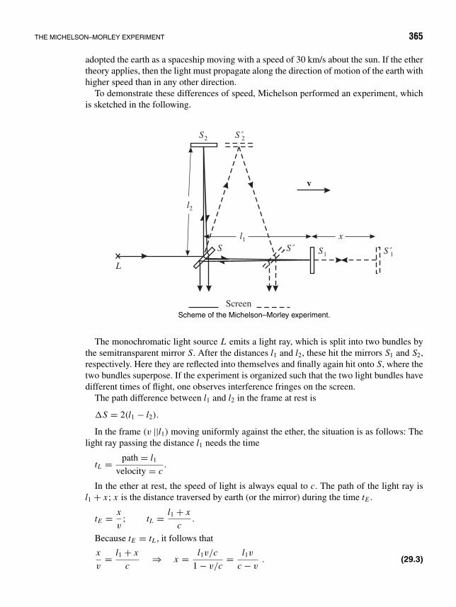
THE MICHELSON–MORLEY EXPERIMENT 365
adopted the earth as a spaceship moving with a speed of 30 km/s about the sun. If the ethertheory applies, then the light must propagate along the direction of motion of the earth withhigher speed than in any other direction.
To demonstrate these differences of speed, Michelson performed an experiment, whichis sketched in the following.
S2
S1
l1 x
l2
S 2
S 1S S´
L
Screen
v
Scheme of the Michelson–Morley experiment.
The monochromatic light source L emits a light ray, which is split into two bundles bythe semitransparent mirror S. After the distances l1 and l2, these hit the mirrors S1 and S2,respectively. Here they are reflected into themselves and finally again hit onto S, where thetwo bundles superpose. If the experiment is organized such that the two light bundles havedifferent times of flight, one observes interference fringes on the screen.
The path difference between l1 and l2 in the frame at rest is
S = 2(l1 − l2).
In the frame (v ||l1) moving uniformly against the ether, the situation is as follows: Thelight ray passing the distance l1 needs the time
tL = path = l1
velocity = c.
In the ether at rest, the speed of light is always equal to c. The path of the light ray isl1 + x ; x is the distance traversed by earth (or the mirror) during the time tE .
tE = x
v; tL = l1 + x
c.
Because tE = tL , it follows that
x
v= l1 + x
c⇒ x = l1v/c
1 − v/c= l1v
c − v. (29.3)

366 RELATIVITY PRINCIPLE AND MICHELSON–MORLEY EXPERIMENT 29
xl1
S1 S 1S
v
The path of the light moving ↑↑ with respect to the direction of flight is l1 + x .
If we now consider the light ray moving back, the path traversed by the light ray equalsl1 − x ′. x ′ is the distance traversed by the oncoming earth during the time t ′
E = x ′/v.
S´ S 1S1
v
l1 x
l1- ´x
S
The path of the light moving ↑↓ with respect to the direction of flight is l1 − x . The background shoulddenote the ether, in which the light was supposed to propagate.
The backmoving light ray needs the time t ′L = (l1 − x ′)/c. Because t ′
E = t ′L , it follows
that
x ′
v= l1 − x ′
c⇒ x ′ = l1v/c
1 + v/c= l1v
c + v. (29.4)
The total distance passed by the light ray is
s1 = l1 + x + l1 − x ′. (29.5)
By inserting x and x ′ (from (29.3) and (29.4)) into equation (29.5), we obtain
s1 = 2l1 + l1v
c − v− l1v
c + v
and after rewriting, we get
s1 = 2l1
1 − v2/c2.
We now consider the path of rays of l2: While the ray is running to S2, the time
t = y
v=√
l22 + y2
c(29.6)

THE MICHELSON–MORLEY EXPERIMENT 367
passes. On the way back the ray needs the same time, that is, it covers the same distance ason the way forward. From there it follows that
s2 = 2√
l22 + y2. (29.7)
y
S S´
l2
S 2
The path of the light moving ⊥ with re-spect to the direction of flight.
We first determine y2 from (29.6):
y2
v2= l2
2 + y2
c2.
Solving for y2 yields
y2 = (v2/c2) l22
1 − v2/c2.
Inserting y2 into (29.7) yields
s2 = 2
√l22 + (v2/c2) l2
2
1 − v2/c2,
s2 = 2l21√
1 − v2/c2.
The path difference between s1 and s2 in the moving frame becomes
s = s1 − s2 = 2l1
1 − (v/c)2− 2l2√
1 − (v/c)2; (29.8)
the difference of the transit times is correspondingly (the propagation speed of light in theether is always equal to c)
t = s
c= 2
c
(l1
1 − (v/c)2− l2√
1 − (v/c)2
). (29.9)
If the experimental set-up is rotated by −90, l1 turns to the direction of l2, and l2 to thedirection of l1, that is, l2 points along the direction of motion of earth. The light ray coversthe distance l2 faster than before the 90 rotation, and the distance l1 is traversed slower.For (v ||l2) an analogous expression results, namely
s = s1 − s2 = 2l1√1 − (v/c)2
− 2l2
1 − (v/c)2. (29.10)
This would cause a shift of the interference fringes, because
s − s = (2l1 + 2l2) ·(
1
1 − (v/c)2− 1√
1 − (v/c)2
)≈ (l1 + l2)
(v
c
)2.
If, on the contrary, the frame is at rest (v = 0), then s ′ in the rotated frame is equalto s in the nonrotated frame, namely the interference fringes are not shifted. Michelsonobserved, however, that also for v = 0 no shift of the interference fringes arises whenrotating the apparatus.

368 RELATIVITY PRINCIPLE AND MICHELSON–MORLEY EXPERIMENT 29
This result might be understood if the speed of light were c = ∞. According to (29.8),one then would have s = s = 2(l1−l2) for both orientations of the Michelson apparatus.Then there were no shift of the interference fringes. But it is known that c = 300, 000 km/s.Hence this explanation is ruled out.
Because the Michelson experiment did not show any shift of the interference fringes andit would be unreasonable to assume the ether to follow the complicated motion of earth,Einstein3 set up the following postulates to explain the result of the Michelson–Morleyexperiment:
The speed of light in vacuum has the same magnitude in all uniformly moving reference frames.
In this case the difference of the light paths s1 − s2 = 2l1 − 2l2 is independent ofthe orientation of the Michelson apparatus. If the speed of light is actually the same nomatter whether the observer is moving toward the light source or away from it, alwayss = s1 − s2 = 2l1 − 2l2 and also s = s1 − s2 = 2l1 − 2l2, hence s − s = 0.Then there is no shift of the interference fringes, so to speak a priori. Moreover, Einsteinpostulated the relativity principle:
3Albert Einstein, physicist, b. March 14, 1879, Ulm—d. April 18, 1955, Princeton (N.J.). He grew up inMunich, then moved to Switzerland at the age of 15 years. As a “technical expert of third class” of the patentoffice at Bern he published in 1905 three highly important papers in Vol. 17 of the Annalen der Physik.
In his Theory of the Brownian Motion Einstein gave a direct and final proof of the atomistic structure of matteron a purely classical base. In the treatise “On the electrodynamics of moving bodies” he founded the special theoryof relativity, based on a penetrating analysis of the concepts of space and time. From this theory he concluded afew months later on the general equivalence of mass and energy, expressed by the well-known formula E = mc2.In the third paper Einstein extended the quantum theorem of M. Planck (1900) to the hypothesis of light quantaand thereby made the decisive second step in the development of quantum theory, which immediately implies theduality conception wave – particle. The idea of light quanta was considered by most physicists as being too radicaland was accepted with much scepticism. The swing of opinion came only after the proposition of the theory ofatoms by N. Bohr (1913).
In 1909 Einstein was appointed as professor at Zurich University. In 1911 he went to Prague; in 1912 again toZurich to the Eidgenossische TH. In 1913 he was called to Berlin as full-time member of the Prussian Academyof Sciences and head of the Kaiser Wilhelm Institute for Physics. In 1914/15 he founded the general theory ofrelativity, starting from the strict proportionality of heavy and inert mass. The successful check of the theoreticalprediction by the British expedition for observing the solar eclipse in 1919 made him publicly known far beyondthe circle of experts. His political and scientific opponents tried to organize a campaign against him and the theoryof relativity, which, however, remained meaningless. The Nobel Committee nevertheless considered it advisableto award the Nobel Prize for Physics of the year 1921 to Einstein not for the proposition of the theory of relativitybut rather for his contributions to quantum theory.
As of 1920 Einstein tried to create a “unified theory of matter,” which should comprise besides gravitation alsoelectrodynamics. Even then when H. Yukawa had shown that besides the gravitation and electrodynamics thereexist still other forces, Einstein continued his efforts that remained however without a final success. Although hehad published in 1917 a landmark paper on the statistical interpretation of quantum theory, he later brought aboutserious objections against the “Copenhagen interpretation” by N. Bohr and W. Heisenberg, which originated inhis philosophical world view.
Offenses because of his Jewish origin caused Einstein in 1933 to resign his academic positions in Germany. Hefound a new sphere of activity in the United States at the Institute for Advanced Studies in Princeton. Einstein’slast life period was clouded by the fact that he—being all his life a convinced pacifist—had given the impetusto build the first American atomic bomb, initiated by a letter of August 2, 1939, commonly written with otherscientists to President Roosevelt, that was motivated by fear of German aggression [BR].

THE MICHELSON–MORLEY EXPERIMENT 369
In all uniformly moving frames there hold the same laws of nature.(covariance of the laws of nature)
Henri Poincare, the great French mathematician, statesman, and contemporary of Ein-stein, expressed it as follows: The relativity law states that the laws of physical phenomenashall be the same both for an observer being at rest, as well as for one put into uniformmotion, that is, we have no, and cannot have a possibility to judge whether we are in sucha kind of motion or not.
These requirements, first set up by Einstein, are not necessarily an implication of theMichelson–Morley experiment. On the contrary, many physicists tried to stick to the etherhypothesis by other possible explanations. An example of such an attempt is a hypothesisbrought forward independently by Lorentz and Fitzgerald which is denoted in literaturesomewhat pathetically as “fatal cry of ether.”
The basic idea is that the Maxwell equations hold in and only in the rest frame ofthe ether. Under this premise there result of course modifications of the electromagneticinteraction—additional electric and also magnetic fields—between those charged particlesmoving relative to the ether.
With this assumption Lorentz could prove that a system of charged particles moving insuch a way against the “ether wind” is shortened by the modified electromagnetic forces.4
In order to apply this idea to the Michelson–Morley experiment, one has to get straightin mind that the surrounding matter, and in particular the measuring apparatus, consists ofelectric charges. In this way Lorentz could show that the arm of the device pointing alongthe motion of earth is shortened by just such an amount, that the actually longer transit timeof light along this direction is compensated. As a consequence, one cannot observe changesof the interference patterns when rotating the measuring apparatus, just as is demonstratedexperimentally.
Although this idea cannot be disproved in a simple way, it seems very unlikely that natureapplies such complicated means to keep our absolute state of motion secret from us.
The goal is now, being confronted with the result of the Michelson–Morley experiment,to find transformation equations that mediate the transition between two inertial systemsK and K ′. These transformation equations are called Lorentz transformations; named afterthe Dutch theoretical physicist Hendrik Antoon Lorentz,5 who for the first time derivedthe Lorentz transformation from the Michelson–Morley experiment, but did not realize itsgeneral validity, and hence also not the philosophically new element.
4H.A. Lorentz, De Relative Bewegung van de AARDE en dem Aether, Amsterdam (1892), Vers. 1, p. 74.5Hendrik Antoon Lorentz, Dutch physicist, b. July 18, 1853, Arnheim—d. Feb. 4, 1928, Haarlem. He was
professor in Leiden and since 1912 curator of the cabinet of natural sciences of the Teyler foundation in Haarlem.Lorentz joined the Maxwellian field theory with the electro-atomistic ideas: The most striking success of thistheory is the explanation of the splitting of spectral lines in a magnetic field, detected in 1896 by P. Zeeman.
Lorentz thoroughly treated the relation between electric and optical phenomena in moving bodies, based onthe electron theory, and he gave a first explanation of the result of the Michelson–Morley experiment by assuminga length contraction of the moving body in the direction of motion (Lorentz contraction). He contributed to thedevelopment of the theory of relativity and the quantum theory. After his retirement he was involved as leaderin the scientific project to drain the Zuidersee. In 1902 he was awarded together with P. Zeeman with the NobelPrize for Physics [BR].

30 The LorentzTransformation
Let us consider two systems moving uniformly against each other with the relative ve-locity v: The system (x, y, z, t) and the system (x ′, y′, z′, t ′), and perform the followingthought experiment.
At the time t = t ′ = 0, the origins of the two coordinate frames shall coincide. At thismoment a light shall flash up at the origin of the two coordinate frames.
We follow Einstein’s postulate—stated in order to explain the result of the Michelson–Morley experiment—that the speed of light has the same value c in each coordinate frame,that is, both an observer in the nonprimed system as well as an observer in the primed systemsee a spherical wave propagating with the same velocity c. That the wave is spherical in bothsystems and not an ellipsoidally deformed wave in the moving system (as one might expectat first) can be explained by the postulate of the relativity principle. This is an additionalrequirement set up by Einstein, according to which the state of motion (the velocity ofthe system) cannot be read off from any observation (equation) in any inertial system. Anellipsoidally deformed wave in the moving system or another propagation velocity wouldallow one to establish the state of motion, and thus would violate the relativity principle.Hence the light flash must be a spherical wave in both systems. Thus, the wave front obeysthe equation
S : x2 + y2 + z2 = c2t2 (30.1)
in the nonprimed system and also
S′ : x ′2 + y′2 + z′2 = c2t ′2 (30.2)
in the primed system.Because S specifies the spherical wave in K , the equation S′ shall according to the
relativity principle also specify a spherical wave in K ′. We further postulate that also fora finite space-time distance x2 + y2 + z2 − c2t2 = 0 in the system at rest, there shallbe a corresponding finite space-time distance in the moving system, namely, x ′2 + y′2 +z′2 − c2t ′2 = 0. One situation shall follow from the other, and vice versa. Therefore, S′
370
THE LORENTZ TRANSFORMATION 371
must follow from S; there must exist a corresponding functional relation between theseequations; for example,
x ′2 + y′2 + z′2 − c2t ′2 = F(x2 + y2 + z2 − c2t2, v
)= F(v)
(x2 + y2 + z2 − c2t2
).
In the last step we have written the functional connection as an operator equation.The operator F thereby acts on the combination (x2 + y2 + z2 − c2t2). The functionF(x2 + y2 + z2 − c2t2, v) still might explicitly depend on the space-time coordinatesx, y, z, t (not only in the combination x2 + y2 + z2 − c2t2), and on the relative velocity v ofthe inertial systems, namely, F(x2 + y2 + z2 − c2t2; x, y, z, t, v). In operator notation thisreads F(x, y, z, ct, v)(x2 + y2 + z2 − c2t2). In this case the operator F depends on thespace-time point (x, y, z, ct) and on the velocity v. But we require homogeneity of spaceand time. In other words: Each space-time point (x, y, z, t) shall have equal rights. Thephysical process then cannot depend on x, y, z, and t . This means that F cannot explicitlydepend on the space-time point x, y, z, t , and we obtain F(x2 + y2 + z2 − c2t2, v). More-over, the space shall be isotropic, that is, the function F must not depend on the orientationof v. In particular then it holds that
F(x2 + y2 + z2 − c2t2, v
) = F(x2 + y2 + z2 − c2t2, −v
),
or in operator form
F(v)(x2 + y2 + z2 − c2t2
) = F(−v)(x2 + y2 + z2 − c2t2
).
But because K is related to K ′ just as K ′ is to K , there must hold with the same function F :
x2 + y2 + z2 − c2t2 = F(−v)(x ′2 + y′2 + z′2 − c2t ′2)
= F(v)(x ′2 + y′2 + z′2 − c2t ′2) (30.3)
= F(v)F(v)(x2 + y2 + z2 − c2t2
).
This is only possible if the operator F means multiplication by ±1. The negative signis excluded because in the limit v → 0 all primed quantities continuously turn into thenonprimed ones. The only remaining possibility is
x ′2 + y′2 + z′2 − c2t ′2 = x2 + y2 + z2 − c2t2. (30.4)
This relation was derived for light waves, and for these it is actually trivial. It is nowgeneralized in the following sense:
The transformation between the two systems K and K ′ shows similarities with a rotationof the coordinate frame in a three-dimensional space: Under a rotation the magnitude ofthe position vector r2 = x2 + y2 + z2 remains conserved; under a Lorentz transformationthe quantity s2 ≡ x2 + y2 + z2 − c2t2 is conserved analogously.
We refer the reader to the subsequent considerations in the context of equation (30.43)!In other words: We now interprete the relation (30.4) in a more general sense, that is,we don’t assume its validity to be restricted to light sources only, but require that thespace-time length of the space-time vector x, y, z, ct remains unchanged under Lorentztransformations.

372 THE LORENTZ TRANSFORMATION 30
In order to get more insight on the relation of the Lorentz transformation to a rotation,we first consider the rotation of a three-dimensional coordinate frame.
Rotation of a three-dimensional coordinate frame
To get a relation between the vector r ′ in the rotated frame S′ and the vector r in the frameS, one adopts for simplicity orthogonal coordinate frames, where r and r′ of course alwaysdescribe the same physical points:
r → r′.
A unit vector in the primed frame must be representable by a linear combination of theunit vectors in the nonprimed frame. One obtains the following system of equations:
e′1 = R11e1 + R12e2 + R13e3,
e′2 = R21e1 + R22e2 + R23e3, (30.5)
e′3 = R31e1 + R32e2 + R33e3.
In matrix notation the three equations read⎛⎝ e′1
e′2
e′3
⎞⎠ =⎛⎝ R11 R12 R13
R21 R22 R23
R31 R32 R33
⎞⎠ ·⎛⎝ e1
e2
e3
⎞⎠ . (30.6)
For one of the equations one may also write
e′i =
3∑k=1
Rikek, i = 1, 2, 3. (30.7)
Let its inversion read as follows:
ei =3∑
k=1
Uike′k, i = 1, 2, 3. (30.8)
To get an idea of what the coefficients Rjk are, we multiply equation (30.7) by em :
e′i · em =
3∑k=1
Rikek · em . (30.9)
Because we have restricted ourselves to an orthogonal system, it holds that
ei · ek = δik .
This means
e′i · em = Rim = cos(e′
i , em).
Just in the same way, (30.8) implies
ei · e′k = Uik = Rki . (30.10)

ROTATION OF A THREE-DIMENSIONAL COORDINATE FRAME 373
Thus, the inverse rotation matrix is the transposed (permuted indices) of the originalmatrix R (compare to Example 6.6).
The coefficients represent the cosines of the angles between the corresponding primedand nonprimed coordinate axes. Such a cosine is also called direction cosine.
From e′i · e′
j = δi j it follows because of (30.7) that
δi j =3∑
k,k ′=1
Rik Rjk ′ek · ek ′ =3∑
k=1
Rik Rjk . (30.11)
This is the row orthogonality of the matrix Ri j . The column orthogonality
3∑k=1
Rki Rkj = δi j (30.12)
follows from the row orthogonality of the Uik utilizing (30.10), namely, Uik = Rki .For a vector r we have
r =3∑
i=1
xi ei .
Because we have required that the vectors r and r′ shall describe the same physical point,we have r = r′. The vector is kept fixed in space; the base frame rotates. Hence
3∑i=1
x ′i e
′i =
3∑i=1
xi ei .
Multiplying this equation by e′k yields
3∑i=1
x ′i e
′i · e′
k =3∑
i=1
xi ei · e′k .
We have ei · e′k = Rki and e′
i · e′k = δik , from which it follows that
x ′k =
3∑i=1
Rki xi ,
or after renaming the indices
x ′i =
3∑k=1
Rik xk, (30.13)
and analogously the inversion
xi =3∑
k=1
Uik x ′k =
3∑k=1
Rki x′k . (30.14)
Thus, the transformation equation for the components is completely analogous to thetransformation equation for the unit vectors (equations (30.7), (30.8)).

374 THE LORENTZ TRANSFORMATION 30
Taking into account (30.13) and (30.14), for the normalization of r in both frames itresults that
|r|2 = x2 + y2 + z2 = x ′2 + y′2 + z′2,or
3∑i=1
x2i =
3∑i=1
x ′2i . (30.15)
Inversely, from the invariance of the magnitude of a vector it follows according to (30.15)that the underlying transformation (30.13) and (30.14) must be an orthogonal transfor-mation (i.e., (30.11) and (30.12) must hold). This will be proved in the following forfour-dimensional vectors, starting from equation (30.17).
The Minkowski space1
In order to point out further analogies between a rotation in 3D space and the Lorentztransformation, we have to change to a four-dimensional space. This 4D space is calledMinkowski space. We introduce the four coordinates
x1 = x, x2 = y, x3 = z, x4 = ict.
A vector in the Minkowski space will be called four-vector. The position vector reads
r = x1e1 + x2e2 + x3e3 + x4e4.
The Minkowski space is an orthogonal space. The orthogonality relations
ei · ek = δik, i, k = 1, 2, 3, 4,
hold. By introducing these coordinates, the propagation of a flash of light as describedby (30.1)
x2 + y2 + z2 − c2t2 = 0
1Hermann Minkowski, b. June 22, 1864, Aleksotas (near Kaunas)—d. Jan. 12, 1909, Gottingen. Minkowskigot his school leaving certificate in Konigsberg (Kaliningrad) at the age of 15 years. Still during his college daysin Konigsberg and Berlin he won in 1883 the Great Prize of the mathematical sciences of the Academy at Pariswith a paper on quadratic forms. In 1885 Minkowski did his doctorate in Konigsberg, followed by his Habilitationin 1887 in Bonn, and since 1892 was appointed professor in Bonn, Konigsberg, and Zurich, since 1902 inGottingen. His most important achievement is the “geometry of numbers,” which he developed, allowing him toobtain number-theoretical results by means of geometric methods. These investigations naturally led him also toresearch on the foundations of geometry. He also contributed significantly to theoretical physics, in particular toelectrodynamics, which deeply influenced the development of the special theory of relativity.

THE MINKOWSKI SPACE 375
may be written in a simpler form, namely,
4∑j=1
x2j = 0.
The expression
4∑i=1
x2i (30.16)
is the square of the magnitude (square of normalization) of the position vector in theMinkowski space. The particular feature is that the normalization of a four-vector may alsobe negative. We have seen by (30.4) that this normalization is conserved under a Lorentztransformation, that is, for Lorentz transformations
4∑i=1
x ′2i =
4∑k=1
x2k . (30.17)
holds. This important relation is no additional, intuitively found postulate. It may beconcluded from the covariance of the light flashes (30.1) and (30.2). This will soon becomeevident: The starting points for determining the Lorentz transformation are equations (30.1)and (30.2). They express the covariance (equality of phenomena) of the spherical light wavein uniformly moving coordinate frames. Hence we look for a coordinate transformationbetween x ′
i (x ′, y′, z′, ict ′) and xk(x, y, z, ict) that converts (30.1) into (30.2), and viceversa. In analogy to the three-dimensional rotations, we try with a linear transformation
x ′n =
4∑j=1
αnj xj , (30.18)
or written out⎛⎜⎜⎜⎝x ′
1
x ′2
x ′3
x ′4
⎞⎟⎟⎟⎠ =
⎛⎜⎜⎜⎝α11 α12 α13 α14
α21 α22 α23 α24
α31 α32 α33 α34
α41 α42 α43 α44
⎞⎟⎟⎟⎠ ·
⎛⎜⎜⎜⎝x1
x2
x3
x4
⎞⎟⎟⎟⎠ , (30.19)
where the αnj constitute the transformation matrix. That the transformation must be linearmay be understood as follows: Linear transformations are the only ones that map a straightline in one frame again on a straight line in other frames. In more general transformationsit would happen that a uniform motion appears as accelerated motion in another inertialsystem. This would contradict the relativity principle. The matrix of a transformation thatconserves the magnitude (30.16) of the position vector is an orthogonal matrix, that is, therow vectors or the column vectors are orthogonal to each other. The matrix αik is such anorthogonal matrix.

376 THE LORENTZ TRANSFORMATION 30
We may realize that by replacing in the relations
4∑k=1
x2k = 0,
4∑i=1
x ′2i = 0
the primed coordinates by
x ′i =
4∑k=1
αik xk, x ′i =
4∑=1
αix. (30.20)
By introducing
x ′2i =
4∑=1
4∑k=1
αikαixk x
in (30.2), the requirement that (30.2) follows from (30.1) and vice versa implies conditionsfor the αik :
0 =4∑
i=1
x ′2i =
4∑i=1
4∑=1
4∑k=1
αikαixk x
=4∑
=1
4∑k=1
(4∑
i=1
αikαi
)xk x
!=4∑
k=1
x2k .
That means that
4∑i=1
αikαi = 1 for k = ,
4∑i=1
αikαi = 0 for k = .
must hold. This is written briefly as
4∑i=1
αikαi = δk. (30.21)
Hence, the column orthonormality for the matrix (αik) holds. The row orthonormalityalso follows from equations (30.1) and (30.2) by starting from the transformation inverseto (30.20)
xi =4∑
k=1
bik x ′k . (30.22)

THE MINKOWSKI SPACE 377
From
0 =4∑
i=1
x2i =
4∑i=1
4∑k,=1
bikbix ′k x ′
!=
4∑k=1
x ′2k ,
it then follows analogously that
4∑i=1
bikbi = δk,
or after renaming the indices
4∑k=1
bki bk = δi. (30.23)
Hence, the bik-matrix is orthonormal also with respect to the columns. But now the bik
from (30.22) are related to the αik from (30.20), because from (30.20) and (30.22) it followsthat
x ′i =
4∑k=1
αik xk =4∑
k=1
4∑=1
αikbkx ′
⇒4∑
k=1
αikbk = δi. (30.24)
A comparison of (30.23) and (30.24) yields
αik = bki , (30.25)
namely, the matrix bki is the transposed αik-matrix. Insertion into (30.23) yields
4∑k=1
αikαk = δi,
and a further renaming of indices yields
4∑i=1
αkiαi = δk. (30.26)
This is the row orthonormality of the matrix (αik). Although we have performed theseconsiderations for the four-dimensional space, each individual step also holds in N dimen-sions. Hence, the relations (30.21) and (30.26) also hold in N dimensions.
With the column orthogonality (30.21) and the row orthogonality (30.26), it follows ingeneral that always∑
i
x ′2i =
∑i
x2i .
This is the invariance of the “magnitude” of the space-time distance under Lorentztransformations (30.15). Hence, this relation (30.15) holds not only for zero vectors (light

378 THE LORENTZ TRANSFORMATION 30
vectors)—that is, those for which∑
x2i = 0—but for all vectors in the Minkowski space,
hence also for those with∑
i x2i = 0. One says: It holds for all four-vectors. Later the
concept of four-vector will be further specified.We now turn to the explicit determination of the Lorentz transformation. In the following
consideration the frames K and K ′ are moving against each other only in the x1-direction.The x ′
1-direction is chosen parallel to the x1-direction; also the x2- and x ′2- or x3- and
x ′3-directions are chosen parallel (see the figure). In this simple case it must be y′ = y,
z′ = z. Moreover, because of the homogeneity of space, the values of x ′1 and x ′
4 must notdepend on x2 and x3 because the choice of the coordinate origin in the x2, x3-plane has nophysical meaning. The Lorentz transformation therefore simplifies to
y
y´
x´
x
v
Two inertial systems of equal ori-entation move with relative veloc-ity v along the z-axis.
x ′1 = α11x1 + 0 + 0 + α14x4, (30.27)
x ′2 = 0 + x2 + 0 + 0, (30.28)
x ′3 = 0 + 0 + x3 + 0, (30.29)
x ′4 = α41x1 + 0 + 0 + α44x4. (30.30)
The αjn may now be determined by the already knownorthonormality conditions (30.21) and (30.26). One hasrow orthonormality
α211 + α2
14 = 1, (30.31)
α241 + α2
44 = 1, (30.32)
α11α41 + α14α44 = 0, (30.33)
and column orthonormality
α211 + α2
41 = 1, (30.34)
α214 + α2
44 = 1, (30.35)
α11α14 + α41α44 = 0. (30.36)
From (30.27), it results that
x ′1 = α11x1 + α14x4 = α11
(x1 + α14
α11x4
)= α11
(x1 + α14
α11ict
).
Now we consider the coordinate origin of K ′. There x ′1 = 0; thus
0 = α11
(x1 + α14
α11ict
)⇒ x1 = −α14
α11ict.
For the velocity it holds that
v = x1 = −α14
α11ic ⇒ α14
α11= i
v
c≡ iβ with β = v
c. (30.37)
According to (30.31),
α211 + α2
14 = 1,

THE MINKOWSKI SPACE 379
α211
(1 + α2
14
α211
)= 1,
α211
(1 − β2
) = 1,
α11 = 1
±√1 − β2.
For low velocities the relativistic mechanics must turn into the Newtonian mechanics.But there x ′
1 = x1,; hence α11 = 1. Therefore, we find the limit
β → 0:1
±√1 − β2→ 1.
From there it follows that only the positive sign holds. We therefore conclude
α11 = 1√1 − β2
⇒ α14 = iβ√1 − β2
.
From (30.32) and (30.35), we obtain
α214 = α2
41,
α14 = ±α41, (30.38)
and from (30.33) it follows that
α44 = −α11α41
α14= ∓α11 = ∓ 1√
1 − β2. (30.39)
The sign may be fixed by a similar consideration as that above. We have
x ′4 = α41x1 + α44x4
orict ′ = α41x + α44ict.
For
v → 0 ⇒ t ′ → t
and for
β → 0 ⇒ 1√1 − β2
→ 1.
Again only the positive sign holds. This implies
α44 = 1√1 − β2
.
From the relation (30.39)
α44 = +α11

380 THE LORENTZ TRANSFORMATION 30
and equation (30.38), we obtain
α14 = −α41;hence
α41 = −iβ√1 − β2
.
The sign again may be determined directly, just as above. A compilation (relative motionof the two frames only in x-direction) leads to the transformation matrix:
(αik) =
⎛⎜⎜⎜⎜⎜⎜⎜⎝
1√1 − β2
0 0iβ√
1 − β2
0 1 0 0
0 0 1 0−iβ√1 − β2
0 01√
1 − β2
⎞⎟⎟⎟⎟⎟⎟⎟⎠. (30.40)
The Lorentz transformation equations (30.27) to (30.30) therefore read
x ′ = x√1 − β2
− v√1 − β2
t,
y′ = y,
z′ = z,
t ′ = t√1 − β2
− v/c2√1 − β2
x . (30.41)
A quick glance at these equations shows that for v c, that is, v → 0 and/or c → ∞,the Lorentz transformation (30.41) turns into the Galileo transformation (29.1). Actually,for v → 0 both coordinate frames become identical (x ′ = x , y′ = y, z′ = z, t ′ = t), and forc → ∞ the Lorentz transformations (30.41) turn into the known Galileo transformations
x ′ = x − vt, z′ = z,
y′ = y, t ′ = t (30.42)
(compare Chapter 17, section on inertial systems).
Definition of the four-vector
Four numbers x1, x2, x3, x4 = ict that, with the base vectors e1, e2, e3, e4 of the Minkowskispace, form a four-vector according to
r = x1e1 + x2e2 + x3e3 + x4e4

THE MINKOWSKI SPACE 381
are called components of the four-vector. They transform under Lorentz transformationsaccording to (30.41). Conversely, if four numbers x ( = 1, 2, 3, 4) transform accordingto (30.41), namely, under Lorentz transformations in a transition from an inertial system Kto another one K ′, then these numbers form the components of a four-vector. They form—briefly spoken—a four-vector. This is similar to the vectors of the three-dimensional space,the components of which must transform under space rotations according to the rotationalmatrix.
We still note that the magnitude of a four-vector remains unchanged under Lorentz trans-formations (30.41). This is evident from equation (30.17) implied by the row and columnorthonormality, but may also be verified explicitly by calculation. Actually, from (30.41) itfollows that
x ′21 + x ′2
2 + x ′23 + x ′2
4 = x ′2 + y′2 + z′2 − c2t ′2
= 1
1 − β2(x − vt)2 + y2 + z2 − c2
1 − β2
(t − v
c2x)2
=[
1
1 − β2− v2/c2
1 − β2
]x2 + y2 + z2 − c2t2
[1
1 − β2− v2/c2
1 − β2
]− t x
[2v
1 − β2− 2v
1 − β2
]= x2 + y2 + z2 − c2t2
= x21 + x2
2 + x23 + x2
4 . (30.43)
Thus, the invariance of the magnitude (30.16, 30.17) of a four-vector generally holds forarbitrary vectors in Minkowski space. Analogously to the rotations of the three-dimensionalspace for which according to (30.15) the magnitude of a vector remains invariant, Lorentztransformations are also denoted as rotations in the Minkowski space. In equation (30.4)the invariance (30.43) served as the starting point of our derivation of the Lorentz transfor-mation. To be more precise, we have postulated the invariance of (30.43) because of thecovariance of the spherical flash of light, (30.1) and (30.2), and constructed the Lorentztransformation from this postulate. We have confirmed this once again for the particulartransformation (30.40).
It is important to note once more that we inferred the Lorentz transformations from thecovariance (and invariance) of the expression
x2 + y2 + z2 − c2t2 = 0 = x ′2 + y′2 + z′2 − c2t ′2 .
Vectors of this kind are called light vectors or better zero vectors. The propagation of lightis described by such a zero vector. But now we point out that these Lorentz transformationskeep also arbitrary (i.e., not only zero-type) four-vectors invariant in magnitude.
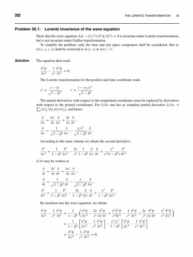
382 THE LORENTZ TRANSFORMATION 30
Problem 30.1: Lorentz invariance of the wave equation
Show that the wave equation ψ − (1/c2) (∂2ψ/∂t2) = 0 is invariant under Lorentz transformation,but is not invariant under Galileo transformation.
To simplify the problem, only the time and one space component shall be considered, that is,ψ(x, y, z, t) shall be restricted to ψ(x, t) or ψ(x ′, t ′).
Solution The equation then reads
∂2ψ
∂x2− 1
c2
∂2ψ
∂t2= 0.
The Lorentz transformation for the position and time coordinate reads
x ′ = x − vt√1 − β2
, t ′ = t − vx/c2√1 − β2
.
The partial derivatives with respect to the nonprimed coordinates must be replaced by derivativeswith respect to the primed coordinates. For ∂/∂x one has as complete partial derivative ∂/∂xi =∑
j (∂x ′j/∂xi )(∂/∂x ′
j ), and hence
∂
∂x= ∂x ′
∂x
∂
∂x ′ + ∂t ′
∂x
∂
∂t ′ ,
∂
∂x= 1√
1 − β2
∂
∂x ′ − v/c2√1 − β2
∂
∂t ′ .
According to the same scheme we obtain the second derivative:
∂2
∂x2= 1
1 − β2
∂2
∂x ′2 − 2v
c2
1
1 − β2
∂
∂x ′∂
∂t ′ + v2
c4(1 − β2)
∂2
∂t ′2 .
∂/∂t may be written as
∂
∂t= ∂t ′
∂t
∂
∂t ′ + ∂x ′
∂t
∂
∂x ′ ,
∂
∂t= 1√
1 − β2
∂
∂t ′ − v√1 − β2
∂
∂x ′ ,
∂2
∂t2= 1
1 − β2
∂2
∂t ′2 − 2v
1 − β2
∂
∂x ′∂
∂t ′ + v2
1 − β2
∂2
∂x ′2 .
By insertion into the wave equation, we obtain
∂2ψ
∂x2− 1
c2
∂2ψ
∂t2= 1
1 − β2
(∂2ψ
∂x ′2 − 2v
c2
∂2ψ
∂x ′∂t ′ + v2∂2ψ
c4∂t ′2 − 1
c2
∂2ψ
∂t ′2 + 2v
c2
∂2ψ
∂x ′∂t ′ − v2
c2
∂2ψ
∂x ′2
)= 1
1 − β2
[∂2ψ
∂x ′2 − 1
c2
∂2ψ
∂t ′2
]− v2/c2
1 − β2
[∂2ψ
∂x ′2 − 1
c2
∂2ψ
∂t ′2
]= ∂2ψ
∂x ′2 − 1
c2
∂2ψ
∂t ′2 = 0.

GROUP PROPERTY OF THE LORENTZ TRANSFORMATION 383
Hence, the invariance under the Lorentz transformation is proved. This result may be obtained morequickly by noting that the four-gradient
∇ = ∂
∂x1e1 + ∂
∂x2e2 + ∂
∂x3e3 + ∂
∂x4e4
is a four-vector, and therefore the four-scalar product
∇ · ∇ = ∂2
∂x21
+ ∂2
∂x22
+ ∂2
∂x23
+ ∂2
∂x24
= ∂2
∂x2+ ∂2
∂y2+ ∂2
∂z2− 1
c2
∂2
∂t2.
must be a Lorentz invariant.We still investigate the wave equation with respect to the Galileo transformation. The Galileo
transformation reads
x ′ = x − vt, t ′ = t.
The partial derivatives are related by
∂
∂x= ∂x ′
∂x
∂
∂x ′ + ∂t ′
∂x
∂
∂t ′ ,∂
∂t= ∂t ′
∂t
∂
∂t ′ + ∂x ′
∂t
∂
∂x ′ ,
∂
∂x= ∂
∂x ′ ,∂
∂t= ∂
∂t ′ − v∂
∂x ′ ,
∂2
∂x2= ∂2
∂x ′2 ,∂2
∂t2= ∂2
∂t ′2 + v2 ∂2
∂x ′2 − 2v∂
∂t ′∂
∂x ′ .
Insertion into the equation yields
∂2ψ
∂x2− 1
c2
∂2ψ
∂t2= ∂2ψ
∂x ′2 − 1
c2
∂2ψ
∂t ′2 − v2
c2
∂2ψ
∂x ′2 + 2v
c2
∂2ψ
∂t ′∂x ′
= 0 = ∂2ψ
∂x ′2 − 1
c2
(∂
∂t ′ − v∂
∂x ′
)/
2ψ.
Obviously the wave equation is not invariant under the Galileo transformation. It is noteworthy, andwe may be surprised in retrospect that the Lorentz transformations, as those coordinate transformationswhich keep the wave equation invariant, were not detected long before Einstein. After all, thewave equation was known since Maxwell. Obviously, basic discoveries mostly are not made in astraightforward way.
Group property of the Lorentz transformation
A nonvoid set G of elements G = g0, g1, g2, . . . with gi , gk, gj ∈ G and a combinationlaw (⊗) are called a group if they have the following properties:
1. The combination (⊗) is an inner combination that to each pair of elements gi , gk ∈ Gassigns a uniquely determined element gj = gi ⊗ gk out of G.
2. The associative law (gi ⊗ gj ) ⊗ gk = gi ⊗ (gj ⊗ gk) holds.

384 THE LORENTZ TRANSFORMATION 30
3. There exists a unit element g0 in G with the property
g0 ⊗ gi = gi ⊗ g0 = gi for all gi ∈ G.
4. To each gi ∈ G there exists an inverse element g−1i also belonging to G and satisfying
gi ⊗ g−1i = g0.
The set G has now the Lorentz transformations as elements (set of operations—asan operation one considers here the transition from one coordinate frame to a secondcoordinate frame moving with uniform relative velocity v with respect to the first frame);the combination means a successive application of the Lorentz transformations. As far ascondition (1) is concerned, this means that the Lorentz transformation from K to K ′′ isequivalent to the successive application of two transformations from K to K ′ and from K ′ toK ′′. For sake of simplicity, here we again consider only particular Lorentz transformationsin x1-direction with parallel axes of K , K ′, and K ′′.
Transformation from K to K ′:
x ′σ =
4∑µ=1
ασµ(β1)xµ,
with
ασµ(β1) =
⎛⎜⎜⎜⎜⎜⎜⎜⎜⎜⎝
1√1 − β2
1
0 0iβ1√
1 − β21
0 1 0 0
0 0 1 0−iβ1√1 − β2
1
0 01√
1 − β21
⎞⎟⎟⎟⎟⎟⎟⎟⎟⎟⎠.
The transformation matrix from K ′ to K ′′ is
x ′′ =
4∑σ=1
ασ (β2)x ′σ .
ασ (β2) is composed just as ασµ(β1), with the only difference that v1 and β1 are to besubstituted by v2 and β2, respectively. For the transformation from K to K ′′ it now resultsthat
x ′′ =
∑σ
ασ (β2)∑
µ
ασµ(β1)xµ (, σ, µ = 1, 2, 3, 4)
=∑σ,µ
ασ (β2)ασµ(β1)xµ
=∑
µ
αµ(β)xµ,
where we have set αµ(β) = ∑σ ασ (β2)ασµ(β1) .

GROUP PROPERTY OF THE LORENTZ TRANSFORMATION 385
The expression∑
σ ασ (β2)ασµ(β1) simply means a matrix multiplication. In order tocalculate αµ(β), we will determine the individual coefficients of this matrix. For example:
α11(β) = α11(β2)α11(β1) + α12(β2)α21(β1) + α13(β2)α31(β1) + α14(β2)α41(β1),
α11(β) = 1√1 − β2
2
1√1 − β2
1
+ β2 · β1√1 − β2
2
√1 − β2
1
= 1√(1 − β2
2 − β21 + β2
1β22 )/(1 + β1β2)2
= 1√1 − [(β1 + β2)/(1 + β1β2)]2
= 1√1 − β2
,
with
β = β1 + β2
1 + β1β2. (30.44)
From here we already get a prescription for the addition of velocities, namely
v = v1 + v2
1 + v1v2/c2. (30.45)
In the subsequent text this “addition theorem” of velocities still shall be derived directlyby another method. The other coefficients of the matrix αik(β) may be determined in thesame manner. We finally obtain
αµ(β) =
⎛⎜⎜⎜⎜⎜⎜⎜⎝
1√1 − β2
0 0iβ√
1 − β2
0 1 0 0
0 0 1 0−iβ√1 − β2
0 01√
1 − β2
⎞⎟⎟⎟⎟⎟⎟⎟⎠, (30.46)
where v and β are determined according to (30.45).From there it follows that the velocity of K ′′ against K is equal to the addition of the
velocities of K ′ against K , and of K ′′ against K ′, according to the addition law (30.45)for relativistic velocities. At the same time we see: Two Lorentz transformations appliedsuccessively again yield a Lorentz transformation. This is nothing else but the closureproperty of the set of Lorentz transformations performed successively (condition (1)).
Because of the principal equality of inertial frames K , there is no difference whetherone performs at first a transformation from K to K ′ and subsequently from K ′ to K ′′ orvice versa, that is, the combination “Lorentz transformation” is even commutative; thesuccessive application of Lorentz transformations is arbitrary with respect to the sequence.This can also be seen immediately from (30.44). But be careful! This holds only for Lorentz

386 THE LORENTZ TRANSFORMATION 30
transformations with the same direction of the velocities, thus for inertial frames movingin the same direction.
The second group property, the associativity of the Lorentz transformation, is also ful-filled. This follows by repeated application of equation (30.45), because for the Lorentztransformation with the velocities β1, β2, β3, we get
(L(β1) ⊗ L(β2)) ⊗ L(β3) = L(β),
with
β = (β1 + β2)/(1 + β1β2) + β3
1 + (β1 + β2)β3/(1 + β1β2)= β1 + β2 + β3 + β1β2β3
1 + β1β2 + β1β3 + β2β3
and
L(β1) ⊗ (L(β2) ⊗ L(β3)) = L(β ′),with
β ′ = β1 + (β2 + β3)/(1 + β2β3)
1 + β1(β2 + β3)/(1 + β2β3)= β1 + β2 + β3 + β1β2β3
1 + β1β2 + β1β3 + β2β3.
Obviously, β ′ = β and, therefore, L(β) = L(β ′).But this means
(L(β1) ⊗ L(β2)) ⊗ L(β3) = L(β1) ⊗ (L(β2) ⊗ L(β3)), q.e.d.
The unit element has the form
g0 =
⎛⎜⎜⎜⎝1 0 0 0
0 1 0 0
0 0 1 0
0 0 0 1
⎞⎟⎟⎟⎠ .
It corresponds to the Lorentz transformation from a system onto itself, namely, no changeof the inertial frame. As required, the combination with the unit matrix is commutative(condition (3)).
To any Lorentz transformation there exists an inverse one of the form
v → −v or β → −β,
g−1i j = αi j (−β) =
⎛⎜⎜⎜⎜⎜⎜⎜⎝
1√1 − β2
0 0−iβ√1 − β2
0 1 0 0
0 0 1 0iβ√
1 − β20 0
1√1 − β2
⎞⎟⎟⎟⎟⎟⎟⎟⎠.
Due to the orthogonality of the Lorentz transformation, the inverse element is obtainedby permuting columns and rows in the transformation matrix; this simply means a reflectionat the main diagonal of the matrix. One may easily verify that
∑j αi j (−β)αjk(+β) = δik

GROUP PROPERTY OF THE LORENTZ TRANSFORMATION 387
(condition (4)). Hence, the initially imposed four conditions for the group properties of aset are fulfilled for the set of Lorentz transformations, that is, the Lorentz transformationsform an infinite, continuous group (the number of elements of the set is not restricted).
Problem 30.2: Rapidity
The Lorentz transformation relating the coordinates t, z and t ′, z′ of two coordinate systems S and S′
in uniform relative motion along the z-axis with velocity v = βc is given by
t = +t ′γ + z′βγ,
z = −t ′βγ + z′γ . (30.47)
This transformation is similar in its structure to a rotation in the t, z-plane,
t = +t ′ cos ϕ + z′ sin ϕ,
z = −t ′ sin ϕ + z′ cos ϕ . (30.48)
However, the factors γ and βγ in (30.47) are greater than 1, which can be achieved with the sineand cosine functions only for an imaginary argument ϕ. One can make instead an ansatz for thetransformation using the hyperbolic functions sinh and cosh with a real argument y:
t = +t ′ cosh y + z′ sinh y,
z = −t ′ sinh y + z′ cosh y. (30.49)
The argument y in these transformation equations is called the rapidity.
(a) Calculate the dependence of y from γ and β.
(b) When applying two consecutive rotations, the two rotation angles can simply be added. Checkwhether this relation also holds for the rapidity in the consecutive application of two Lorentztransformations.
Solution (a) Comparision of (30.47) and (30.49) yields
γ = cosh y and γβ = sinh y .
The factor β can thus be obtained as
β = tanh y .
(b) If t ′ and z′ are written as
t ′ = +t ′′ cosh y′ + z′′ sinh y′ ,
z′ = −t ′′ sinh y′ + z′′ cosh y′ , (30.50)
then inserting this in (30.49) yields
t = +t ′′(cosh y cosh y′ + sinh y sinh y′) + z′′(sinh y cosh y′ + cosh y sinh y′),
z = −t ′′(sinh y cosh y′ + cosh y sinh y′) + z′′(cosh y cosh y′ + sinh y sinh y′). (30.51)

388 THE LORENTZ TRANSFORMATION 30
Using the addition theorems of the hyperbolic functions or reducing them to the exponential functionsgives the resulting equations
t = +t ′′ cosh(y + y′) + z′′ sinh(y + y′),
z = −t ′′ sinh(y + y′) + z′′ cosh(y + y′) . (30.52)
This corresponds to a single Lorentz transformation with rapidity
y′′ = y + y′ .
Thus, the rapidity variable is additive for two consecutive Lorentz transformations along the samedirection, in the same way as the rotation angle is additive for two consecutive rotations around thesame axis.
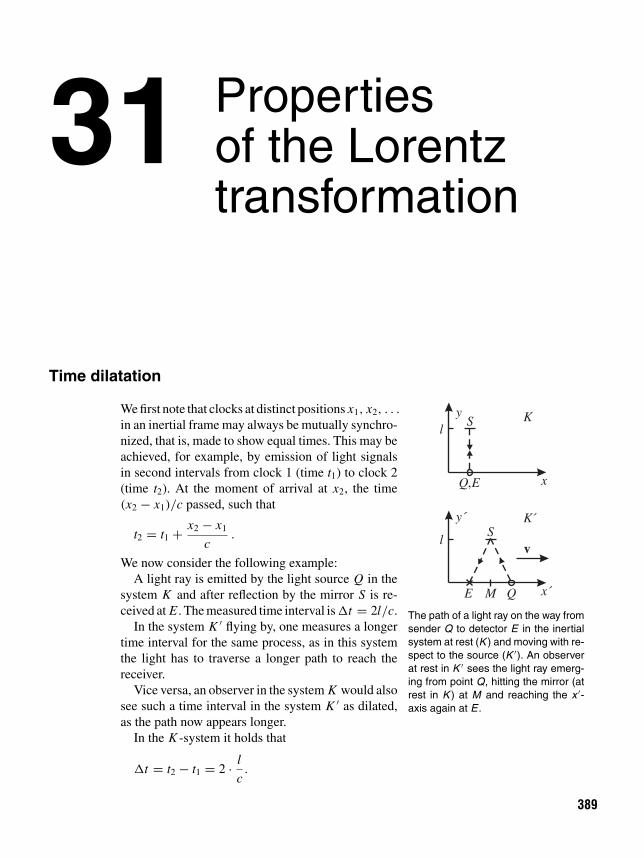
31 Propertiesof the Lorentztransformation
Time dilatation
l
l
y
y´
K
K´
x
x´
S
S
Q E,
E QM
v
The path of a light ray on the way fromsender Q to detector E in the inertialsystem at rest (K ) and moving with re-spect to the source (K ′). An observerat rest in K ′ sees the light ray emerg-ing from point Q, hitting the mirror (atrest in K ) at M and reaching the x ′-axis again at E .
We first note that clocks at distinct positions x1, x2, . . .
in an inertial frame may always be mutually synchro-nized, that is, made to show equal times. This may beachieved, for example, by emission of light signalsin second intervals from clock 1 (time t1) to clock 2(time t2). At the moment of arrival at x2, the time(x2 − x1)/c passed, such that
t2 = t1 + x2 − x1
c.
We now consider the following example:A light ray is emitted by the light source Q in the
system K and after reflection by the mirror S is re-ceived at E . The measured time interval is t = 2l/c.
In the system K ′ flying by, one measures a longertime interval for the same process, as in this systemthe light has to traverse a longer path to reach thereceiver.
Vice versa, an observer in the system K would alsosee such a time interval in the system K ′ as dilated,as the path now appears longer.
In the K -system it holds that
t = t2 − t1 = 2 · l
c.
389

390 PROPERTIES OF THE LORENTZ TRANSFORMATION 31
After the Lorentz transformation in the system K ′, it holds that
t ′ = t ′2 − t ′
1,
where
t ′ = t − (v/c2) x√
1 − β2
for = 1, 2. We now have x1 = x2 because the light pulse is emitted and received at thesame position in the K -system. Hence the interval is given by
t ′ = t√1 − β2
.
The time interval t in the system at rest corresponds to the time interval t ′ in the movingsystem. For our example it results that
t ′ = 2l
c
1√1 − β2
.
The dilatation of the time intervals by the Lorentz transformation is of course independentof the special definition of the time interval adopted here. If in one system the time Tpassed, an observer moving relative to the system finds that his clock displays the longertime T/
√1 − β2. An observer will consider time intervals in systems moving relative to
him always as dilated. This fact led to the concept of time dilatation.The same result is obtained in a somewhat modified experiment: If signals are emitted
from the same position x in K at the times t1 and t2, they will be received in K ′ with thetime distance
t ′2 − t ′
1 = t2 − (v/c2) x√1 − β2
− t1 − (v/c2) x√1 − β2
= t2 − t1√1 − β2
.
In the system K ′, the signals are emitted at distinct positions x ′1 and x ′
2. We have
x ′1 − x ′
2 = x − vt1√1 − β2
− x − vt2√1 − β2
= v(t2 − t1)√1 − β2
= v(t ′2 − t ′
1).
This phenomenon will be elucidated further by the following example 31.1. It is importantthat the clock in the system at rest (in our case, the system K ) always ticks at the sameposition (x1 = x2) while, on the contrary, in the moving system (in our case, the system K ′)these signals are emitted at distinct positions (x ′
1 = x ′2). This type of measuring process is
the reason for the different values of the observation times in both systems.One may construct, although somewhat artificially, a measurement of the time intervals
in such a way that the moving observer faces a shortening: At the times t1 and t2 in thesystem K at rest there occur two events at all points of a distance that is parallel to thex-axis (flashing of various lamps connected in coincidence – note that this cannot be afluorescent tube). The time distance t ′
2 − t ′1 of the events is measured by means of a moving
clock from the moving coordinate frame.

TIME DILATATION 391
We then have
t ′2 − t ′
1 = t2 − t1 − (v/c2)(x2 − x1)√1 − β2
.
Let the measurement be performed always at the same position in the moving system; hencewe have
x ′2 − x ′
1 = 0 = x2 − x1 − v(t2 − t1)√1 − β2
,
and by elimination of x2 − x1
t ′2 − t ′
1 = (t2 − t1)√
1 − β2.
It is evident that this kind of measuring time intervals, for example, for the decaying muonin the following example, does not apply.
Example 31.1: Decay of the muons
The time dilatation may be proved by means of a cosmic process: The earth is surrounded by anatmosphere of about 30-km thickness screening us off from influences from the universe. If a protonfrom the cosmic radiation hits the atmosphere, π -mesons are produced; several of them decay furtherinto a muon (a “heavy electron”) and a neutrino each. Now one establishes the following: The muonhas a mean lifetime of t = 2 · 10−6 s in its rest system. Classically, according to s = v · t , itmight traverse even with the speed of light only a distance of 600 m. Nevertheless the particle hasbeen recorded at the earth’s surface.
In the relativistic approach, however, this contradiction is resolved: Muons at rest have a mass ofm0 c2 = 108 eV. The “cosmic” muons are created at an altitude of ca. 10 km with a total energy ofE = 5 · 109 eV.
Hence we have
s ′ = vt ′ = vt√1 − β2
= x ′ :
s ′ = vm0c2
m0c2√
1 − β2t = v
m0c2Et.
The expression for the relativistic energy E = m0 c2/√
1 − β2 used here will be derived later on inChapter 33.
t is the lifetime of the muons in their rest system. x ′ is the path of the muon during its lifetimet ′ = t/
√1 − β2 in the moving system (i.e., we and the detector, fixed to the earth). t ′ is
determined by emission of two signals: The first one indicates the creation, the second one the decayof the muon in the moving system K ′.

392 PROPERTIES OF THE LORENTZ TRANSFORMATION 31
To get an upper estimate, we replace v by the speed of light; thus we find
s ′ ≈ 3 · 1010
108· 5 · 109 · 2 · 10−6 cm = 30 km.
More precise measurements1 actually gave a value of 38 km.
Problem 31.2: On time dilatation
We consider a spaceship that moves away from earth with the velocity v = 0.866c. It emits two lightsignals to earth spaced by t ′ = 4 s (spaceship time).
(a) What is the time distance T (earth time) between the two signals arriving on earth?
(b) What distance, measured from earth, did the spaceship cover between emitting the two signals?
(c) A body at rest in the spaceship has the mass m0 = 1 kg. What is its kinetic energy measured fromearth?
Solution (a) We denote the emission of the first and second light flashes as events A and B, respectively. Inthe spaceship frame S′ they have the space-time coordinates (x ′
A, t ′A) and (x ′
B = x ′A, t ′
B = t ′A + t ′);
in the earth-fixed frame S the coordinates (xA, tA) and (xB = xA + x , tB = tA + t). The relationbetween the two coordinate frames is given by
x = γ (x ′ + vt ′), t = γ(
t ′ + v
c2x ′)
,
with γ = (1 − (v/c)2)−1/2 = 2 for x = xA or xB , etc. Therefore,
xA = γ (x ′A + vt ′
A), tA = γ(
t ′A + v
c2x ′
A
),
xB = γ (x ′B + vt ′
B), tB = γ(
t ′B + v
c2x ′
B
),
hence, using x ′B − x ′
A = 0,
xB − xA = x = γ vt ′ , tB − tA = t = γt ′ .
In S the two signals are emitted at the distance t = γt ′. During this time the spaceship movedforward by the distance x . The two light signals arrive at the earth-fixed point x0 at the time TA andTB = TA + T , respectively. TA and TB are calculated as
TA = tA + xA − x0
c, TB = tB + xB − x0
c,
where (xA − x0)/c and (xB − x0)/c represent the transit times of the signals in S from point xA andxB , respectively, to the point x0. Hence
TB − TA = T = tB − tA + 1
c(xB − xA) = t + 1
cx,
1The first experiments of this kind were carried out in the late 1930s and early 1940s; see, e.g., Bruno Rossi,Norman Hilberry, J. Barton Hoag: “The variation of the hard component of cosmic rays with height and thedisintegration of mesotrons,” Phys. Rev. 57 (1940) 461–469, and Bruno Rossi, David B. Hall: “Variation of therate of decay of mesotrons with momentum,” Phys. Rev. 59 (1941) 223–228. The “mesotron” in these papers isthe lepton, which is today known as the muon.

TIME DILATATION 393
that is, the measured time difference between the received signals is composed of the time differencet in S (the emissions), and a transit time difference. With the equations derived above, we have
T = γ(
1 + v
c
)t ′ = (1 + v/c)t ′
√(1 + v/c)(1 − v/c)
=√
1 + v/c
1 − v/ct ′.
With the data of our example, we obtain T = 15 s.(b) The path x covered by the spaceship between the two emissions as seen from earth is
x = γ vt ′ = 2.1 · 109 m.(c) The body has a total mass of m = m0γ = 2 kg and a kinetic energy of Ekin = (m − m0)c2 =
9 · 1016 J, which corresponds to about 0.7% of the total electric energy produced in the United Statesin 1999. The expression for the kinetic energy used here will be substantiated in detail in Chapter 33.
Problem 31.3: Relativity of simultaneity
y y´
y´
xv x´
x´
z z´
z´
Earth Galaxy
tA
tB
A galaxy moving with velocity v perpendic-ular to the distance from earth.
We observe that in a remote galaxy two events A andB happen at the same position within the galaxy. Ingalaxy time the event B happens by 4 s later than theevent A. Further let the distance between earth andgalaxy be practically constant for our problem, thatis, the galaxy shall move with a constant velocity vperpendicular to the visual line earth–galaxy (see fig-ure).
On earth the event B is recorded by 6 s later thanthe event A. Find the velocity |v| of the galaxy relativeto earth.
Solution The coordinate frame in the galaxy is denoted by primed quantities (S′), the earth-fixed frame bynonprimed quantities (S). The event A [B] takes place at galaxy time t ′
A [t ′B], and the signal originating
there is received on earth at the time tA [tB]. According to the condition the signals emitted by thegalaxy from the events A and B traverse the same way to earth, such that the time difference betweent ′ = t ′
B − t ′A = 4 s and t = tB − tA = 6 s is caused by the time dilatation only. Hence:
tB − tA = γ (t ′B − t ′
A)
or
γ = tB − tA
t ′B − t ′
A
= 6
4= 1.5.
From γ immediately follows the velocity v = |v| of the galaxy relative to earth:
γ = 1√1 − v2/c2
, γ 2 = 1
1 − v2/c2.
1 − v2/c2 = 1/γ 2, and v is thus obtained as
v = c
√γ 2 − 1
γ 2= c
√1, 52 − 1
1, 52= 0.75 c.

394 PROPERTIES OF THE LORENTZ TRANSFORMATION 31
Lorentz–Fitzgerald length contraction
A further property of the Lorentz transformation is the length contraction measured undera relative motion of observer and object. Let us consider a rod of length l resting in thenonprimed frame K , and an observer in the moving frame K ′; the frame K ′ moves with arelative velocity v parallel to the rod axis.
The measurement of the length is performed in such a way that the coordinates of the rodends are determined in the observer’s system at the same time (t ′ = 0) and the differenceis formed, l ′ = x ′
2 − x ′1.
According to the Lorentz transformation,
x ′ = x − vt√1 − β2
.
The rod length is then
x ′2 − x ′
1 = x2 − x1 − v(t2 − t1)√1 − β2
. (31.1)
Simultaneity of the reading-off for the observer means t ′2 − t ′
1 = 0; that means
t ′2 − t ′
1 = (t2 − t1) − (v/c2)(x2 − x1)√1 − β2
= 0.
From that we may determine the time interval t2 − t1. If we still set x2 − x1 = l andinvestigate equation (31.1), there results
l ′ = x ′2 − x ′
1 = l√
1 − β2. (31.2)
For the moving observer, the rod resting in K appears to be shortened by the factor√1 − β2z.The cause of the length contraction is again the finiteness of the speed of light. Among the
light rays from the rod ends—exploited in the measurement—which arrive simultaneouslyat the observer’s position, the first one leaves the rod at the time t1; then a time intervalt2 − t1 = vl/c2 passes until the second light ray leaves the other rod end.
Because the rod (or the observer’s frame) is moving farther during this interval, acontraction of the rod is seen by the observer. Because only the relative motion of observerand rod matters, we always get a length contraction, no matter whether the frame of theobserver or that of the rod is considered as being at rest (or moving).
Let the volume of the cube in its rest frame be V = x y z; in the moving frame thevolume is
V ′ = x ′ y′ z′ = x√
1 − β2y z = V√
1 − β2. (31.3)
Thus, the moving observer measures a smaller volume. This measurement proceeds insuch a way that one measures from the moving frame perpendicularly to the direction ofmotion the distances y′ = y and z′ = z, and parallel to the direction of motion thedistance x ′ = x
√1 − β2.

LORENTZ–FITZGERALD LENGTH CONTRACTION 395
y´ y
x´
x∆x
∆y
v
Volume contraction.
The phenomenon that time intervals appear asextended for the moving observer, while space dis-tances appear as shortened, is due to the distinctnature of the measuring process in these cases (inthe case of time measurement, we have already mettwo possibilities leading to dilatation or shortening,respectively).
If the measurement of length were performed byemitting signals at the ends of the distance that aresimultaneous in the resting system, and by determining the position of the signals with themoving rule, then t1 = t2 and
x ′2 − x ′
1 = x2 − x1√1 − β2
.
In this measurement the moving observer would find no contraction but rather a dilatationof the distance. The difference as compared with the earlier prescription of measurementlies in the fact that the two measured values are now recorded simultaneously in the restingframe, but formerly simultaneously in the moving frame.
Problem 31.4: Classical length contraction
Let a rod of length l0 move with constant velocity v along the z-axis of a coordinate frame. Show thatan observer at rest in this frame sees this rod as contracted also “fully without the theory of relativity”if the light propagates with finite velocity (classical length contraction). Hint: One should think abouthow the observer will define the length of the rod.
Solution The observer will conclude on the length of the rod from the light emitted by the beginning and bythe end of the rod, and arriving simultaneously at his position. For simplicity we assume the observerto be at one end of the rod at some instant.
v
B zl~
B´
Because of the finite speed of light c, the observer B sees the end of the rod at an earlier instantτ = l/c at which the rod still was shifted left by the amount vτ . Thus, he finds for the length of therod
l = l − vτ = l − vl
c
⇒ l = l
1 + v/c.

396 PROPERTIES OF THE LORENTZ TRANSFORMATION 31
This is the classical length contraction. However, if the rod is moving toward the observer, thisclassical consideration yields a length dilatation—similar to the situation with the classical Dopplereffect. The classical consideration thus results—depending on the case at hand—in either a lengthcontraction or a length dilatation.
The relativistic consideration, however, yields a length contraction in all cases.
Problem 31.5: On the length contraction
A measuring rule of rest length l moves relative to an observer with the velocity v. The observermeasures the length of the rule to be 2
3 l. Find the velocity v.
Solution We first derive the equation for the Lorentz contraction; according to the Lorentz transformations, itholds that
x ′ = x − vt√1 − β2
. (31.4)
The length of the rule as measured by the observer is then
x ′2 − x ′
1 = x2 − x1 − v(t2 − t1)√1 − β2
. (31.5)
Simultaneity of the reading-off for the observer means that t ′2 − t ′
1 = 0; that is,
t ′2 − t ′
1 = (t2 − t1) − (v/c2)(x2 − x1)√1 − β2
= 0
⇒ t2 − t1 = v
c2(x2 − x1).
With l ′ = x ′2 − x ′
1 and l = x2 − x1, it follows after insertion in (31.5) that
l ′ = l√
1 − β2 . (31.6)
According to the data, l ′ = 23 l. Equation (31.6) then implies√
1 − v2
c2= 2
3.
From there it follows for the velocity that(v
c
)2 = 1 − 4
9= 5
9⇒ v = 0.745 c.
Note on the invisibility of the Lorentz–Fitzgerald length contraction
From the result of the length contraction it has been concluded that an observer would seea cube moving relative to him as a cuboid, and a sphere as an ellipsoid. However, this isnot the case, as we will see now.

NOTE ON THE INVISIBILITY OF THE LORENTZ–FITZGERALD LENGTH CONTRACTION 397
This fallacy has been noted by the Austrian physicist Anton Lampa2 in 1924, but hisshort paper (in German) remained virtually unnoticed. Only in 1959 were Lampa’s mainideas independently rediscovered by James Terrell3.
It turns out that the length contraction of spatial distances along the direction of motionunder distinct methods of observation has distinct consequences. For elucidation we con-sider the optical image of a moving cube produced on a photographic plate parallel to alateral face of the cube.
A AA
D DD
B
B
B
CC
C
l
ll
ll
A D, D DA AB C, B B
a) c)b)
lβ lβl l= 1−β2
l l= 1−β2
v
α
α
Optical appearance of a cube at rest (a) and in uniform motion (b). Figure (c) shows the apparentrotation of the cube by the angle α.
The condition of recording is again the simultaneous arrival of all light in the frame ofthe photographic plate. If the relative velocity v equals zero, we see (for the appropriatearrangement) only the face AB; the lateral faces AD and BC are not visible.
If the cube is moving then, due to the finite speed of light, the light arriving simultaneouslyon the plate has been emitted by the cube at distinct times. Although the record is madeunder the same conditions as in the first case, this implies that the side face AD nowbecomes visible.
A light ray from the point D travels by the time T = l/c longer, that is, it was emittedearlier by this time, than a ray from the point A arriving simultaneously with the first ray.The same holds for the other points of the face AD. During the time l/c, the cube moved
2Anton Lampa, “Wie erscheint nach der Relativitatstheorie ein bewegter Stab einem ruhenden Beobachter?”(How does a moving rod appear to an observer at rest according to the theory of relativity?), Z. Physik 27 (1924)138–148. Anton Lampa, b. Jan. 17 1868, Budapest, Hungary—d. Jan. 27 1938, Vienna. Lampa was a distiguishedexperimentalist working in the field of electrodynamics and electromagnetic properties of matter, and a talentedteacher. The eminent nuclear physicist Lise Meitner was among his students in Vienna. From 1909–1919, Lampawas professor for experimental physics and head of the physics institute at the German University in Prague (nowCzechia). He was one of the first German physicists fully grasping the importance of Einstein’s new special theoryof relativity and managed to get Einstein on his first full professorship, the chair for theoretical physics at theGerman University in Prague, in 1909. After the Great War, Lampa had to resign from his post in Prague andreturned to Vienna. He did hardly any physics research anymore, but committed himself to adult education. Infact, his note on the appearence of a moving rod is his sole physics paper after 1919.
3J. Terrell, “Invisibility of the Lorentz contraction,” Phys. Rev. 116 (1959) 1041–1045.

398 PROPERTIES OF THE LORENTZ TRANSFORMATION 31
farther by the distance s = v · l/c = l · β, namely, the face AD is recorded on the plate asshortened by the factor β. According to the Lorentz–Fitzgerald contraction, the face ABis recorded as shortened by the factor
√1 − β2. From the two-dimensional photoplate one
thus gets the impression that the cube is rotated by the angle α (tan α = γβ = β/√
1 − β2)
and that the body apparently retained its shape.
The visible appearance of quickly moving bodies4
Until the appearance of the paper of James Terrell in 1959, it was generally believed that amoving body seems to contract along the direction of motion by a factor (1 − (v/c)2)1/2—Lampa’s note on this subject seems to have had no impact at all. The passenger of a fastspaceship would see spherical bodies as reduced ellipsoids, which, however, is impossibleaccording to Terrell’s opinion and for the particular case of the sphere has been proved byR. Penrose.5 The reason for that is seen by the following consideration: If we see or takea photograph of an object, then we receive certain quantities of light emitted by the bodythat arrive simultaneously on the retina or on the film. This includes the possibility thatthese quantities of light are not emitted simultaneously by all points of the body. The eye orthe photographic device therefore perceives a distorted image of the moving object. In thespecial theory of relativity, this distortion has the remarkable consequence to compensatethe Lorentz contraction such that the object appears not as distorted but only as rotated.This, however, holds exactly only for bodies that lie within a small solid angle—only thenthe image consists mainly of parallel light pulses.
Optical appearance of a quickly moving cube
To elucidate the situation we consider the image distortion under nonrelativistic conditions,that is, the light propagates with the velocity c in a frame at rest against the observer, andthat the motion of the object does not cause a Lorentz contraction. In the frame of the objectmoving with velocity v, the speed of light along the direction of motion would be c − v,and in the opposite direction it would be equal to c + v.
We first consider a cube of edge length l that moves parallel to an edge and is observedfrom a direction perpendicular to the direction of motion (it is observed from a large distanceto keep the solid angle covered by the cube possibly small). The square ABC D oppositeto the observer is perceived as nondistorted as all points of the face have the same distanceto the observer. The situation is different for the square AB E F being perpendicular to thedirection of motion. If the cube is moving, the face AB E F becomes visible: Due to thetime shift of the light signals from the points E and F , which are emitted by (l/c) seconds
4We follow a paper by V.F. Weisskopf, Physics Today Sept. 1960.5R. Penrose, Cambridge Phil. Soc. 55 (1959) 137.

OPTICAL APPEARANCE OF A QUICKLY MOVING CUBE 399
Direction towardsObserver
A
A
A
D
D
D
C
C
C
B
B
B
FF
F
F´E
E
E
E´v classical
relativistic
Optical appearance of a cube (classical and relativistic).
earlier than the signals from the points A and B, the points E and F are observed with aspatial displacement of (l/c)v at the positions E ′ and F ′.
The face AB E F is thus seen as a rectangle with a height l and a width (v/c) l. Thismeans that the image of the cube is distorted. In a nondistorted image of a rotated cube, bothfaces would appear as shortened; if the face AB E F were shortened by the factor (v/c),the face ABC D should be shortened by the factor (1 − (v/c)2)1/2, while nevertheless theface ABC D appears as a square. Therefore, in the classical consideration, the image of thecube appears as extended in the direction of motion. A similar consideration for a movingsphere shows that it would appear as an ellipsoid extended along the direction of motion bythe factor (1 + (v/c)2)1/2. One gets still considerably more paradox results if the image ofa moving cube in a nonrelativistic world is not considered under an angle of 90 relative tothe direction of motion but under an angle of 180 − α, where α is a very small angle. Wenow look at the object to the left while it moves from the left toward our position. In orderto simplify the consideration we assume v/c = 1. The figure illustrates the new situation.The edges AB, C D, E F are denoted by the numbers 1, 3, 2. We assume that the edge 1emits its light quantum at the moment t = 0. One sees that edge 2 must emit its light muchearlier and edge 3 much later to get a simultaneous arrival at the observer’s position.
Actually edge 2 must emit its light if it reaches the position of the point 2′, which isdefined by the equality of the distances 2′2 and 2′M (the velocity v was assumed to coincidewith the speed of light c!).
2
22´
2
1
1
1,3
3
3 3´
classical
relativistic
αα
M
N
III
III Observer
Optical appearance of a cube moving (nearly) toward the observer.

400 PROPERTIES OF THE LORENTZ TRANSFORMATION 31
The interval 2′2 is the distance traversed by edge 2 between the emission of 1 and 2.The length 2′M is the distance traversed by the light from 2′ to be “in line” with the lightemitted by 1. Both the light as well as the edge move with the speed c; one can see that thedistance 1M is equal to 12 (1M = 12 = l). The corresponding also holds for edge 3. Theintercept theorems imply
3′Nl sin α
= 1N
l cos α= 13′
l= l + 1N
l,
and therefore,
3′N = l sin α (1 − cos α)−1.
Note that 33′ = 1N !The image of the cube is indicated in the figure by the points I, II, III. We see a strongly
deformed cube, with edge 2 to the left of 1, such as if the cube were viewed from backward,and edge 3 far to the right of 1. In the direction of flight there results an extended image;the area between 1 and 2 appears as a square.
The theory of relativity simplifies the situation. It removes the image distortion suchthat there results a nondistorted but rotated image of the object. This may be seen directlyfrom the quoted examples. Let us assume that the cube is observed perpendicularly to itsdirection of motion; the Lorentz contraction reduces the spacing between edges AB andC D by the factor (1− (v/c)2)1/2 and keeps the spacing between AB and E F invariant. Theimage of the face ABC D is thus represented as shortened exactly by the amount needed toyield a nondistorted image of the cube rotated by the angle arcsin(v/c). If the cube moveswith the speed of light toward us (α = 0), then the Lorentz contraction reduces the spacingbetween edges 1 and 3 to zero. The resulting image is a regular square that is identical withthe lateral face AB E F of the cube. In the general case (finite α), the cube is observed asnondistorted, but rotated by an angle of (180 − α).
Basing on the following consideration, we may show that this result is generally validfor any object.
Optical appearance of bodies moving with almost the speed of light
AB
CD
k
The points A, B, . . . emit lightthat arrives at the same timein the plane of the observer.
It is assumed that a bundle of light pulses originating from Npoints of the body moves along the direction of k such thatall light pulses are on a plane perpendicular to k (see figure).This light bundle arrives simultaneously at the observer andcreates the seen shape of the body.
Such a bundle of light rays will be called a “picture.” Un-der nonrelativistic conditions the “picture” does not remainan image when seen from a moving reference system. Thereason is that in a moving frame the plane of the light pulsesis no longer perpendicular to the direction of propagation.In a relativistic world the situation is different. There the

OPTICAL APPEARANCE OF BODIES MOVING WITH ALMOST THE SPEED OF LIGHT 401
“picture” remains an image in any reference frame. The light pulses arrive simultaneouslyat the observer in any reference frame.
This fact may be proved in the following manner. The light pulses are visible, that is,one may imagine them as being embedded in an electromagnetic wave just there wherethis wave has a peak (wave group). It is known that electromagnetic waves are transversein all reference systems, namely, that the front side of the wave or the plane of the wavepeak is perpendicular to the propagation direction in any system (the vectors of the electricand magnetic field oscillate ⊥ to the propagation direction k). It may also be shown thatthe spacing between the light pulses is an invariant quantity. One only has to introduce acoordinate frame, the x-axis of which is parallel to the propagation direction.
The only variable quantity is the direction of propagation—the vector k. The change ofthe propagation direction is given by the aberration relation to be derived in the following.
A light ray that encloses the angle θ with the x-axis is observed under the angle θ′
in aframe moving with the velocity v along the x-axis. The angle θ
′is the angle under which
the observer sees the incident light coming in (see figure). As may be seen from the figure,in the resting frame the light needs the time t = P0 P1/c = P0 P3/(c · sin θ) for traversingthe distance P0 P1.
During this time, point P2 moves to P1. The distance P2 P1 is
P2 P1 = v · t = v
c
P0 P3
sin θ.
y´v
P1 P3
P2
P0
θ´
θ
θ´
θ
y
x´
xDeduction of the relation for the aberration of light.

402 PROPERTIES OF THE LORENTZ TRANSFORMATION 31
Taking into account the relation
P1 P3 = c · cos θ · t = P0 P3 · cot θ
for the distance P2 P3 results in the expression
P2 P3 = P2 P1 + P1 P3 = P0 P3
sin θ
(v
c+ cos θ
).
The nonrelativistic aberration results from the fact that the light is observed under theangle (θ ′)n.r. given by
sin(θ ′)n.r. = sin(π − θ′n.r.) = sin(θ
′)n.r.
= P0 P3√P0 P3
2 + P2 P32
= sin θ√1 + 2(v/c) cos θ + v2/c2
.
Because θ = π − θ , we thereby obtained the relation between θ ′ and θ in the nonrela-tivistic case. To get the functional dependence of the observer angle θ ′ on the angle θ in therelativistic case, one has to take into account that the determined distance P2 P3 in the restframe of the telescope (observer) because of the length contraction has the value P2 P3
′,
which is calculated from the relations
P2 P3′√
1 − v2/c2 = P2 P3
or
P2 P3′ = P2 P3√
1 − v2/c2(31.7)
(see (31.2)). The rest length here is the distance P2 P ′3. It appears in the frame of the resting
light source as P2 P3 and is related with that quantity through (31.2) or (31.7). From therenow results the wanted aberration relation:
sin θ ′ = sin(π − θ′) = sin θ
′ = P0 P3√P0 P3
2 + P2 P3′2
= P0 P3√P0 P3
2 + P0 P32
(1 − (v/c)2) sin2 θ(v/c + cos θ)2
=√
1 − (v/c)2 sin θ
1 + (v/c) cos θ=
√1 − (v/c)2 sin θ
1 − (v/c) cos θ, (31.8)
because θ = π − θ . When changing from the frame “moving observer – light source atrest” to the frame “observer at rest – moving light source,” one has only to replace v → −v
in (31.8), which yields
sin θ ′ =√
1 − (v/c)2 sin θ
1 + (v/c) cos θ. (31.9)

OPTICAL APPEARANCE OF BODIES MOVING WITH ALMOST THE SPEED OF LIGHT 403
Expressed by the angles (compare the figure)
θ ′ = π − θ ′, θ = π − θ, (31.10)
(31.9) finally reads
sin θ ′ =√
1 − (v/c)2 sin θ
1 − (v/c) cos θ. (31.11)
Formally this is the same relation as (31.8), but—and this is important—the angleschanged their meaning: According to (31.10), they are the supplement angles for θ ′, θto 180.
By the way, the inversion of equation (31.11) reads
sin θ =√
1 − (v2/c2) sin θ ′
1 − (v/c) cos θ ′ , (31.12)
which is symmetric to (31.11), that is, only θ and θ ′ are interchanged, as one would expect.From the invariance of the image of a point, we may draw the following conclusions:
The image of a moving point observed under the angle θ ′ is identical with the image of thesame point at rest and observed under the angle θ . We therefore see a nondistorted image ofa moving object (point set) that is virtually rotated by the angle θ ′ − θ . A spherical objecttherefore continues to appear as a sphere.
θ´
θ
π π
ππ/2
12
3
v=0
vc
<<
v c~~
~~ 1– /v c2 2
Illustration of the aberration relation.
This should not be interpreted as nonex-istence of Lorentz contraction. Of course,the Lorentz contraction happens, but it onlycompensates for the extension of the im-age caused by the finite propagation speedof light (see (31.7)). The classically ex-pected image extension is just balanced bythe Lorentz contraction!
It is appropriate to plot the angle θ ′ ac-cording to equation (31.11) as a function ofθ . The figure shows this graph for v = 0 (1),for a small value of v/c (2), and also forv/c ≈ 1 (3). We see that the virtual rota-tion is always negative. This means that onesees also that side of an object that pointsopposite to the direction of motion. In theextremum case v ≈ c, the angle θ ′ is extraordinarily small for all values of θ , except forthose where the angle 180 − θ corresponds to the value (1 − (v/c)2)1/2.
Because for an object moving past the angle θ ranges from 180 to 0, we find that forv ≈ c the front face of the object is visible only in the very beginning. During the oncomingthe object rotates; hence also its face pointing opposite to the direction of motion becomesvisible to us. This state continues until the object leaves us. From that moment one sees theobject from the back. This paradox situation is possibly not so surprising, if we remember

404 PROPERTIES OF THE LORENTZ TRANSFORMATION 31
the fact that the aberration angle amounts to almost 180 for v ≈ c. If the object is movingtoward our position, we see the light from it coming up to us.
Light intensity distribution of a moving isotropic emitter
The situation becomes more transparent if we consider the light distribution as seen fromthe observer in more detail. Let us assume the moving object to emit rays that are isotropicin their own reference system, namely, their intensity is independent of the emission angleθ . This radiation does not at all appear as isotropic in the frame of an observer at rest(laboratory system): Here it seems to be concentrated in the forward direction. For v ≈ c,most of the emitted light seems to form a very small angle θ ′ with the direction of motion.This effect implies that an isotropic radiation appears as if almost the entire radiation wereemitted into a spotlight cone.
The connection between the angular distribution I (θ) of the radiation intensity in therest frame of the light source and the angular distribution I (θ ′) in the rest frame of theobserver (in which the light source is moving) is obtained as follows: We consider a lightbeam that in the frame of the light source is emitted with the intensity I (θ) under the angleθ and passes an infinitesimal area element d F = r2 sin θdθdϕ (compare the figure).
r´
r
y´
y
x´
x
d ´F
dF
θ´
θ
–v
Angular distribution of light in two frames in relative motion to each other.
In the frame of the observer, this light beam is detected with the intensity I (θ ′) under theangle θ ′. It thereby passes through the infinitesimal area element d F ′ = r ′2 sin θ ′dθ ′dϕ′. Itis clear that the quantity of light passing through d F ′ in the frame of the observer must bethe same as that passing through d F in the frame of the light source,
I (θ)d F = I (θ ′)d F ′.
It is also clear that the increment dϕ′ = dϕ, because here dϕ is perpendicular to the imageplane (compare the figure) and therefore is not affected by the transformation between themoving and the resting frame.

LIGHT INTENSITY DISTRIBUTION OF A MOVING ISOTROPIC EMITTER 405
Moreover, we may choose r = r ′ = 1: The factor r2(r ′2) in the equation for d F(d F ′)describes only the geometric widening of the light beam if we don’t let it pass at a defineddistance (here r = r ′ = 1) from the coordinate origin through the test area. We thereforeobtain
I (θ) sin θdθ = I (θ ′) sin θ ′dθ ′.
The aberration formula (31.9) thereby provides the relation between θ and θ ′. We use(31.9) because the light source shall move relative to the observer (see the following figure).
dθ ′
dθ=
√1 − v2/c2
1 + (v/c) cos θ,
dθ
dθ ′ =√
1 − v2/c2
1 + (v/c) cos θ ′ .
Thus, we obtain as ratio of the radiation intensities
I (θ)
I (θ ′)= sin θ ′ dθ ′
sin θ dθ= K (θ) = 1 − v2/c2
(1 + (v/c) cos θ)2(31.13)
orI (θ ′)I (θ)
= sin θ dθ
sin θ ′ dθ ′ = K (θ ′) = 1 − v2/c2
(1 + (v/c) cos θ ′)2. (31.14)
θ´19
15
10
5
1
K( )1+ /1 /
v cv c−
1 /1+ /−v c
v c
v c/ = 0,9
K
10K
0 π/2 π θ´
~ ( 2 1)(1 / )− − c v
1 / 1− 1− c v( )/−v c2 2
The relation of intensities K (θ ′) as function of the angle of observation θ ′.
The last formula (31.14) is the really interesting one because it expresses the intensityI (θ ′) in the frame of the resting observer as function of his observation angle θ ′. I (θ) is theintensity distribution of the light source in the frame of the resting source. As was alreadystated above, we will assume the source as isotropic, namely, we set I (θ) = constant.

406 PROPERTIES OF THE LORENTZ TRANSFORMATION 31
Here θ ′ is the observation angle with forward direction at θ ′ = π . The function K (θ ′) isplotted versus θ ′ in the figure. We see the maximum in the forward direction (θ ′ = π) andthe minimum in the backward direction (θ ′ = 0).
At high velocities v/c = 1, the maximum becomes extremely sharp, such that the mainfraction of the radiation is emitted within a small angle about θ ′ = π . The beam width isobtained from
1 − (v/c)2
(1 + (v/c) cos θB)2= 1
2
1 + v/c
1 − v/c= 1
2K (π).
Here, θB is the so-called half-maximum angle: At the angle θB , the intensity of the forward-directed “spotlight cone” is reduced to half of the maximal intensity, which is reached atθmax = π . Rewriting of the first equation yields
√2(
1 − v
c
)= 1 + v
ccos θB .
One immediately sees that not every value of v is allowed, for example, v = 0 leads tothe contradiction
√2 = 1. The reason is that for v = 0 there is no change of the intensity
I (θ) = constant due to aberration. Hence there is no forward-directed “spotlight cone” thatreaches half of its maximum intensity ratio at θB .
It is evident that the light source must move at least with such a speed that θB may take atleast the value 0 (at backward angles the intensity ratio reaches only half of the maximumvalue). With cos θ = cos 0 = 1, it then follows that v must take at least the value
v = c ·√
2 − 1√2 + 1
≈ 0.172c.
For larger velocities one may evaluate a θB ∈ [0, π ] as solution of the equation
cos θB = c
v(√
2 − 1) − √2.
For high velocities θB ≈ π , or θB = π − ϑ , where ϑ is a small positive angle. Withcos (π − ϑ) = − cos ϑ ≈ −1 + 1
2θ2 = −1π + 12 (π − θB)2, it follows that
θB ≈ π −√
2(√
2 − 1)( c
v− 1
),
that is, the width takes about the value√
2(√
2 − 1)(c/v − 1). The value of θ ′ for whichK (θ ′) = 1 (θ ′ = θ1) may also be given in a straightforward way. Then
1 −(v
c
)2
(1 + v
ccos θ1
)2 = K (θ1) = 1
must hold, that is,
cos θ1 = c
v
(√1 −
(v
c
)2 − 1
).

DOPPLER SHIFT OF QUICKLY MOVING BODIES 407
For high velocities again θ1 ≈ π , namely, by means of an argument analogous to thatabove, one may determine θ1 as
θ1 ≈ π −√√√√1 − c
v
(1 −
√1 −
(v
c
)2)
.
Doppler shift of quickly moving bodies6
y
x
v
k
k
θ
The light source is at rest, while the ob-server moves by with velocity v .
An observer moving with the velocity v observesin the moving frame (i.e., in his rest frame) lightof frequency ω′ = 2π′ emitted by a resting lightsource with frequency ω = 2π.
We are working in the frame of the lightsource K .
The light source emits light of frequency ω
(period T ) under an angle θ against the x-axis. Inthe figure each bar perpendicular to k indicatesa “wave peak” of the light wave. What is thesituation for the moving observer?
1
2
θ
y
xx1 x2
ab
Instant t1: The first wave peak arrives and isdetected.
cT
1
2
θ
y
xx1
Instant t2: The second wave peak ar-rives and is detected.
6We also refer to the detailed work of Hasselkamp, Mandry, and Scharmann, Zeitschrift fur Physik A289(1979) 151.

408 PROPERTIES OF THE LORENTZ TRANSFORMATION 31
However, the observer moved with v toward the wave peak (therefore, he will measurea shorter spacing between the wave peaks, and, consequently, measure the ultraviolet shiftof the Doppler effect).
There holds (sure): x2 −x1 = v(t2 − t1). (The observer meanwhile moved with v in the x-direction.) Moreover (compare figure): λ = cT = a+b = c(t2 − t1)+(x2 −x1) cos(π −θ).a is the distance covered by the wave peak 1 during the time t2 − t1; b follows from thegeometry of the right-angled triangle.
Therefore,
cT = c(t2 − t1) + v(t2 − t1) cos(π − θ)
⇔ T = (t2 − t1)(
1 − v
ccos θ
).
But t2 − t1 is just the time difference that would be measured by the observer as a period:It is just the time he sees passing between the arrival of two wave peaks—apart from thefact that he measures with a clock that is at rest in his moving frame. Thus one still has toLorentz-transform:
vy´
x´θ´
θ´θ x
y
true Position apparent Position
The real and apparent position of thelight source.
Path 1:
t ′2 − t ′
1 = γ(
t2 − t1 − v
c2(x2 − x1)
)= γ (t2 − t1)
(1 − v2
c2
)= 1
γ(t2 − t1),
thust2 − t1 = γ (t ′
2 − t ′1).
Path 2:
t2 − t1 = γ(
t ′2 − t ′
1 + v
c2(x ′
2 − x ′1))
(in the primed frame the point of arrival of the two wave peaks is always the originx ′
2 = x ′1 = 0)
t2 − t1 = γ(t ′2 − t ′
1
).
Both arguments yield the same result (as it must be). We now denote t ′2 − t ′
1 = T ′, that is,the period measured by the moving observer in his frame.
We get
T = γ T ′(
1 − v
ccos θ
)or
T ′ = 1
γT
1
1 − v
ccos θ

DOPPLER SHIFT OF QUICKLY MOVING BODIES 409
y´
y´
y´
y
y
y
x´
x´
x´
x
x
x
v
v
v
K
K
K´
K
K
K
θ´
θ´
θ´
θ
θ
θ
t t= <01
t t t= = =02
t t= >03
0
0
0
I
I
I
I´
I´
I´
or
ω′ = γω(
1 − v
ccos θ
)This is the Doppler formula!
Actually ω′ is larger if the observermoves toward the light source, becausethen θ ∈ [π/2, π ] ⇔ cos θ ∈ [−1, 0].The additional factor γ then providesthe Doppler shift caused by the aber-ration: Even if the light source emitsits radiation under θ = 90, the ob-server measures a higher frequency.The reason is: The observer still musttilt his telescope against the directionof motion because of the relativisticaberration. He therefore virtually seesthe light source coming up to him (al-though it just passes him; see figure).This implies the (relativistic) Dopplereffect!
This important relation still may beunderstood in another way: If we con-sider the light as a plane wave7
ψ = ψ0ei(K·r−ωt),
and generalize the wave number vec-tor to a four-vector (compare to Chap-ter 33)
Kµ =(
K, iω
c
),
ψ = ψ0ei∑
µKµxµ
,
we may investigate the behavior of the four-wave number vector under Lorentz trans-formations and also calculate the Doppler effect. Kµ must be a four-vector. The phase∑4
µ=1 Kµxµ in the plane wave must be a scalar, because otherwise the interference prop-erties in distinct Lorentz systems would be different. But this cannot be true. Because nowxµ is a four-vector, Kµ also must be a four-vector.
7Plane waves can be described by functions of the type 0 cos(K · r − ωt). The planes of constant phaseφ = K · r − ωt are planes that are moving in the direction of K with the velocity v = ω/|K| = ω/K . Weuse the complex exponential in our description of the plane wave for technical reasons only. The imaginary parti0 sin(K · r − ωt) is also a plane wave. It is carried along, but not used.

410 PROPERTIES OF THE LORENTZ TRANSFORMATION 31
In the frame I ′ moving with v, the plane wave is observed in the x ′, y′-plane under theangle θ ′ against the x ′-axis with a frequency ω′. The wave number vector Kµ of the planewave in the resting frame I of the light source is related to the four-vector K ′
µ via a Lorentztransformation (compare to (30.40)):
K ′µ = ω′
c
⎛⎜⎜⎜⎝cos θ ′
sin θ ′
0
i
⎞⎟⎟⎟⎠ =
⎛⎜⎜⎜⎝γ 0 0 iβγ
0 1 0 0
0 0 1 0
−iβγ 0 0 γ
⎞⎟⎟⎟⎠ ω
c
⎛⎜⎜⎜⎝cos θ
sin θ
0
i
⎞⎟⎟⎟⎠ .
That this transformation correctly describes the situation of the figure may easily be realizedby considering the corresponding transformation of the position vector,
x ′ = γ (x − βct),
y′ = y,
z′ = z,
t ′ = γ
(t − β
cx
).
From there it follows that the origin of the coordinate frame I ′(x ′ = y′ = z′ = 0) hasthe x-coordinate x = βct = vt in the frame I , as it must be because the frame I ′moves relative to I with v in the x-direction (and we have synchronized the times att = t2 = t ′ = 0). Conversely, the origin of the frame I (x = y = z = 0) has the x ′-coordinate x ′ = −γβct = −βct ′ = −vt ′ in the frame I ′, which is evident because theframe I moves relative to I ′ with v in the (−x ′)-direction.
For the first and fourth components of the K ′µ-vector, we obtain
ω′
ccos θ ′ = ω
c(γ cos θ − βγ ),
iω′
c= ω
c(−iβγ cos θ + iγ ).
Solving the system of equations for ω′ and cos θ ′ yields
cos θ ′ = −β + cos θ
1 − β cos θ, cos θ = β + cos θ ′
1 + β cos θ ′ ,
ω′ =√
1 − β2
1 + β cos θ ′ ω, ω′ = √K (θ ′)ω.
Here K (θ ′) is the quantity already defined in equation (31.14). As is easily checkedby using the relation sin θ ′ = √
1 − cos2 θ ′, the first line is equivalent to equation (31.8)(see above). The dependence of the frequency ω′ of the received light on the observationangle θ ′ coincides with the relation obtained by geometric consideration. This is the wantedaberration relation.

DOPPLER SHIFT OF QUICKLY MOVING BODIES 411
The aberration of the light emitted by fixed stars was first discovered and explained byJames Bradley8 (1728).
To ensure that the light from a far remote star hits the eye of the observer moving withthe earth, the observer must tilt his telescope according to the aberration relation.
We shall get this phenomenon straight to our mind by a particular case of the aberrationrelation. Let us assume that the k-vector in the resting frame I of the light source just takesthe angle θ = π/2 against the x-axis, that is, that the light is emitted just perpendicularto the x-axis and parallel to the y-axis. This corresponds to the case t = t2 = t ′ = 0 inthe above figure. We now ask under which angle θ ′ the observer in the moving frame I ′receives the light. According to the aberration relation, one then has (cos θ = cos π/2 = 0)
cos θ ′ = −β,
namely, θ ′ > π/2, as is also indicated in the figure. But this means that the observer hasto tilt his telescope against the direction of motion to get the k′-vector pointing along thetelescope axis (see the following figure).
v
θ´θ
Star
Observerat rest
Observerin motion
Explaining the aberration of the light from fixed stars.
We still discuss the Doppler shift. If the observer moves from a wide distance directlytoward the light source, the light must be emitted under θ = π for him to receive it.According to the above formula, then also θ ′ = π and
ω′ =√
1 + β
1 − βω > ω,
8James Bradley, British astronomer, b. end of March 1693, Sherborne (near Dorchester)—d. July 13, 1762,Chalford (near Gloucester). Bradley was professor of astronomy at Oxford, then, following Edmund Halley onthis post, astronomer royal and professor at Greenwich Observatory. In 1728, while searching for the parallax ofstars, Bradley discovered the aberration of star light and used this observation to calculate the speed of light. In1748, he confirmed the nutation of the earth’s axis, which had been predicted by I. Newton. Bradley compiled atGreenwich a catalog with the precise locations of more than 3200 stars.
412 PROPERTIES OF THE LORENTZ TRANSFORMATION 31
that is, the received frequency ω′ is larger than the genuine light frequency ω. If the observerat far distance moves off the light source, then θ = θ ′ = 0 and
ω′ =√
1 − β
1 + βω < ω,
that is, the received frequency ω′ is smaller than the genuine light frequency. The particularcase θ = π/2 is also of interest. We have seen that then cos θ ′ = −β (aberration formula),and therefore
ω′ = 1√1 − β2
ω = γω > ω. (31.15)
Although the light was emitted under θ = π/2, it is received in the observer’s frameunder θ ′ > π/2, that is, such as if the observer moved toward the light source. This isaccompanied with the usual Doppler shift to higher frequencies!
We now describe what will be seen if an object moves away with nearly the speed oflight: We first observe under an angle close to θ ′ = 180. Here we see the front side ofthe object whereby, due to the strong Doppler shift, a high intensity and a shift to veryhigh frequencies are observed. One looks into the spotlight beam of the radiation. If theobservation angle reaches the magnitude θ ′ = π − (1 − (v/c)2)
1/2, the color changes to
lower-frequency values, the intensity decreases, and the object seems to rotate.If θ ≈ π − 21/4(1 − (v/c)2)1/2, thus is still close to 180, we are beyond the “spotlight
ray”; the color now has significantly lower-frequency values than in a frame convected withthe object. The object has now rotated completely, and we see its side pointing opposite tothe direction of motion. The front side is invisible because all rays emitted forward in themoving frame join into the small “spotlight cone.” The images seen at angles smaller thanπ − 21/4(1 − (v/c)2)
1/2remain essentially unchanged until the object disappears.
All these considerations are only then exact if the object is confined within a very smallsolid angle. Only then the image nearly consists of parallel light pulses. At larger valuesof the solid angle, we expect distinct rotations for the various fractions of the image thatlead to image distortions. Whatsoever, Penrose has shown that the image of a sphere has acircular circumference also at large observation angles.
Relativistic space-time structure—space-time events
In a four-dimensional coordinate frame, as was introduced for the mathematical descriptionof the Minkowski space, we may no longer operate with the concept “position” as in three-dimensional space. We therefore introduce the concept “event” to stress the equality ofspatial and time coordinates. The four-dimensional space of three position coordinates andone time coordinate is frequently denoted simply as space-time.
A mass point that moves or is at rest relative to its inertial frame is described as a functionof time and space, thus as a curve in space-time. This curve in the Minkowski space iscalled a world line.

RELATIVISTIC PAST, PRESENT, FUTURE 413
ctA
B
v c=
x
World line of a point at rest (a), inaccelerated motion (b), and mov-ing at the speed of light (c).
The time behavior of a point being at rest (A) (repre-sentation in the two-dimensional subspace of the Minkowskispace), as well as that of a mass point moving relative toan inertial frame (B) may be described geometrically asis shown in the graph. The reciprocal slope of the curvespecifies the velocity of a moving mass point.
At an angle of 45 against the x-axis one has the lineof light; it holds that
tan α = ct
x= 1 ⇒ c = x
t.
A curve bent to the right represents a mass pointgetting faster; a curve bent to the left represents a per-manently decelerated point. Because the speed of lightcannot be exceeded, the smallest possible slope equals 1.
Relativistic past, present, future
In the Minkowski space the length element ds2 = dx2 + dy2 + dz2 − c2dt2 is invariant
Light cone
ds2 = 0ds2 < 0
ds2 < 0
x
ct
Past
Future
Present ds2 > 0
ds2 > 0
Two-dimensional subspace of the four-dimensional space-time.
against Lorentz transformations. Because of thecoordinate ict in the four-dimensional space-timecompound, the length element is no longer positive-definite. The following cases may be distinguished:
(a) ds2 > 0This distance is called spacelike since the “spa-
tial” part of the length element is larger than thetime part, that is,
dx2 + dy2 + dz2︸ ︷︷ ︸spatial part of ds2
> c2dt2︸ ︷︷ ︸time part of ds2
If, for example, two events happen at the sametime but at distinct positions, then dx2 + dy2 +dz2 = 0 and c2dt2 = 0.
For an observer at the origin of the above frame, those events that have a space-likedistance to him cannot be found out because of the finite speed of light. No informationmay be obtained from this region. The speed of the information transfer would have to belarger than the speed of light. The spacelike distance remains spacelike under any Lorentztransformation.
(b) ds2 < 0Such distances are called timelike, because the time part of ds2 dominates, that is,
c2 dt2 > dx2 + dy2 + dz2.
One is dealing with events that happened already or will happen, thus events that we“have seen” or “shall see” if we understand ourselves again as observers at the origin.

414 PROPERTIES OF THE LORENTZ TRANSFORMATION 31
Events from the past may be identified by their aftereffects; conversely, we may influencethe future by events that have lasting effects. The region of the Minkowski space for whichds2 > 0 remains inaccessable to us.
The timelike distance specifies that dx2 + dy2 + dz2 < c2 dt2. In this case there exists aLorentz transformation for which ds2 = ds ′2 = −c2 dt ′2 and dx ′2 + dy′2 + dz′2 = 0. Thismeans that these events may be observed.
(c) ds2 = 0This is the region of the light cone; the region of the greatest possible signal velocity
that characterizes the zero elements. The spatial part of the length element is equal to thetime part, namely
dx2 + dy2 + dz2 = c2 dt2. (31.16)
Vectors dr with ds2 = dr · dr = 0 are also called zerolike or lightlike. They lie on a conein four dimensions, because we would have to draw four coordinate axes for a completedescription of this hypersurface.
For a resting observer at the position x = 0 at the instant t = 0 all those events constitutethe present which also happen at the time t = 0. The past corresponds to the events witht < 0, the future to all events with t > 0. This convention is independent of the position.The observer has access only to those events that for him are in the timelike region.
As simultaneous one declares all those events for which in any moving frame it holdsthat t ′
1 = t ′2. Simultaneous with the event x ′ = 0, t ′ = 0 for an observer moving with v are
the events
t ′ = t − (v/c2)x√1 − β2
= 0,
that is, all events for which in a resting frame
t = v
c2x .
holds. Every event in the interval −x/c < t < x/c (the hatched region in the last figure—the present) may for an observer moving with the appropriate velocity between ±c besimultaneous with the event at x ′ = 0, ct ′ = 0. In other words: Two events that lie in aspacelike distance to each other can be made simultaneous. For this purpose one has onlyto describe these events in an inertial system with the appropriate velocity.
The causality principle
The causality principle of classical mechanics states that an event cannot happen earlierthan its cause, that is, the triggering event must have taken place earlier than the resultingone.
If this principle shall continue to hold in the theory of relativity, there must not exist aninertial system in which the causal relation of the events is inverted.

THE LORENTZ TRANSFORMATION IN THE TWO-DIMENSIONAL SUBSPACE OF THE MINKOWSKI SPACE 415
As an example of an appropriate course, one may take the blackening of a photographicplate following a light flash. If the causing event happens in the system K at the time t1at the position x1, the resulting event at the later time t2 > t1 at the position x2, then anytransformation to a K ′-system must satisfy
t ′2 − t ′
1 ≥ 0.
As the speed of light represents the greatest possible signal velocity, for the causalrelation in the frame K
c ≥ x2 − x1
t2 − t1
holds; that means
c(t2 − t1) ≥ (x2 − x1).
For the time difference in the frame K ′ moving with v relative to K ,
t ′2 − t ′
1 = c(t2 − t1) − (v/c)(x2 − x1)
c√
1 − β2.
holds. Because now c(t2 − t1) ≥ (x2 − x1) and v/c ≤ 1, there follows that for all inertialframes
t ′2 − t ′
1 ≥ 0.
The order of sequence of causally related events is therefore independent of the referenceframe; the causality principle remains valid in relativistic mechanics.
The Lorentz transformation in thetwo-dimensional subspace of the Minkowski space
The length contraction and the time dilatation may well be visualized in this subspace.We distinguish between the real coordinates x(x ′) and ct (ct ′) on the one hand, and theMinkowski coordinates x(x ′) and ict (ict ′) on the other hand. At first the representation isin real coordinates:
The relation between two systems moving relative to each other is given by
x ′ = x − (v/c) · ct√1 − β2
, ct ′ = ct − (v/c) · x√1 − β2
. (31.17)
To get the position of the primed coordinate axes, we set
x ′ = 0 = x − v
cct (t ′-axis)
and
ct ′ = 0 = ct − v
cx (x ′-axis).

416 PROPERTIES OF THE LORENTZ TRANSFORMATION 31
The inclination angle α of the ct ′-axis against the ct-axis is determined by tan α =x/ct = v/c. The inclination angle β of the x ′-axis against the x-axis is given by tan β =ct/x = v/c. Hence α = β, that is, both axes are inclined by the same angles against thecorresponding coordinate axes of the resting system (x, ct) (compare the figure).
For a complete representation of Lorentz contraction and time dilatation we consider thebehavior of the unit scales on the two axes. Because s2 = s ′2 = x2 − c2t2 = x ′2 − c2t ′2 isinvariant under Lorentz transformation, x2 − c2t2 = 1 represents the invariant unit scale inall Lorentz systems. The associated world lines are equilateral hyperbolas with light coneas asymptote (compare the figure).
x´
ct ct´
1
0
α
α
x ct=
1= –= ´ – ´
x c tx c t
2 2 2
2 2 2
xB A1
B´A
Graphical representation of the Lorentz trans-formation in real coordinates.
These hyperbolas cut out the unit scales onthe axes. The unit scale in the (x, ct)-frame(K ) is O A. An observer at rest in the frame(x ′, ct ′) (K ′) sees it with the length O B ′,that is, shorter than his own scale O A′. Themeasuring signals are namely emitted at thepoints x = 0 and x = 1 in K ; the endpointsof the distance 01 in K are represented bythe world lines x = 0 and x = 1 (parallelsto the t-axis). This corresponds to the unitdistance at rest in K . In the frame K ′ at thesame time (t ′ = 0) a picture is taken, that is,the intersection point of the x ′-axis with theworld lines of the points 0 and 1 resting in Kis determined.
Conversely, an observer at rest in K sees the scale O A′ as O B, that is, shorter than hisown scale O A. Hence the Lorentz contraction is a mutual effect. The mutual control of theclocks proceeds in the corresponding manner.
A more convenient geometrical representation of time dilatation and Lorentz contractionthat makes the comparison with unit scales unnecessary is obtained by using the coordinatex4 = ict instead of the time coordinate ct . Equations (31.17) then turn into
x ′1 = (x1 + iβx4)√
1 − β2, x ′
2 = x2 , x ′3 = x3 , x ′
4 = (x4 − iβx1)√1 − β2
. (31.18)
The associated Lorentz transformation is
αµ =
⎛⎜⎜⎜⎝γ 0 0 iγβ
0 1 0 0
0 0 1 0
−iγβ 0 0 γ
⎞⎟⎟⎟⎠ . (31.19)
Here 1/√
1 − β2 = γ has been abbreviated. αµ is an orthogonal transformation andmay therefore be represented as
x ′1 = cos ϕ x1 + sin ϕ x4, x ′
4 = − sin ϕ x1 + cos ϕ x4. (31.20)

THE LORENTZ TRANSFORMATION IN THE TWO-DIMENSIONAL SUBSPACE OF THE MINKOWSKI SPACE 417
By comparison of coefficients of (31.18) and (31.20), we get
cos ϕ = γ ≥ 1 and sin ϕ = iβγ or tan ϕ = iβ. (31.21)
Because cos ϕ = γ ≥ 1, ϕ must be an imaginary angle. The trigonometric functionscos ϕ, sin ϕ, tan ϕ, cot ϕ for imaginary arguments ϕ = iα (α real) are defined by thecorresponding series expansions. For example, cos ϕ = cos(iα) = 1−(iα)2/2!+(iα)4/4!−· · · = 1 + α2/2! + α4/4! + · · · > 1. Hence, cos iα is larger than 1 and may even diverge to
ϕ
x4
x1
x 1
x 4P
Graphical representation of theLorentz transformation in Minkowskicoordinates.
infinity in the limit α → ∞. Correspondingly, sin iα =iα/1! − (iα)3/3! + · · · = i(α/1! + α3/3! + · · ·), namely,purely imaginary. In fact, the series expansions of thetrigonometric functions sin and cos for imaginary argu-ment iα yield the hyperbolic functions, sinh and cosh. Ifwe compare with Example 30.2, we see that α is just therapidity introduced there.
Because orthogonal transformations are angle-conserving,(31.20) may be represented as a simple rotation of the axes(compare figure).
ϕ ϕ
ϕ
L0x1
x4x 4 x 1
L 0T0
L
L
b)
a)
T
Lorentz transformation in Minkowski coor-dinates.
Lorentz contraction and time dilatation be-come evident from the figure by geometrical con-siderations:
One has
L = L0
cos ϕ= L0
γ
andT = T0 cos ϕ = T0γ. (31.22)
When using x4 = ict , the geometric relationsfor the Lorentz contraction and time dilatationmay be read off directly from the diagram. It is not necessary to investigate the behavior ofthe unit scales! But be careful! Only the geometry is correctly reproduced by the drawing:For Example, T in the diagram is smaller than T0, but actually it holds that
T = T0√1 − β2
; thus T > T0.
The relation for the length contraction and time dilatation is mutual for both inertialframes. This fact has been explained for the length contraction by the cases (a) L0 rests inK ′, and (b) L0 rests in K in the above figure: In both cases one always measures in thecorrespondingly other (moving) system
L = L0
cos ϕ= L0
√1 − β2.
The length measurement in a coordinate frame is always performed at the same instant; forexample, in case (a) at fixed x4, and in case (b) at fixed x ′
4.

418 PROPERTIES OF THE LORENTZ TRANSFORMATION 31
Problem 31.6: Lorentz transformation for arbitrarily oriented relative velocity
Let S be an inertial frame. Let a frame S′ move with uniform velocity v against S. Show that theLorentz transformation from S to S′ looks as follows:
x′ = x⊥ + γ[x|| − β(ct)
], γ = 1√
1 − β2,
ct ′ = γ [ct − β · x] , β = vc,
with x⊥ and x|| denoting the components of x perpendicular and parallel to β, respectively.
Solution (a) If v points in the x-direction, then one gets the well-known relation
x ′ = γ [x − β(ct)], y′ = y, γ = 1√1 − β2
,
ct ′ = γ [ct − βx], z′ = z, β = v
c.
(b) The general Lorentz transformation is then determined by the condition
x′2 − (ct ′)2 = x2 − (ct)2.
This is now fulfilled by the above relations:
x′2 − (ct ′)2 = x2⊥ + γ 2
[x2
|| − 2β x||ct + β2(ct)2 − (ct)2 + 2β x ct − (β x)2]
= x2⊥ + γ 2 = [
(1 − β2)x2|| − (ct)2(1 − β2)
]= x2 − (ct)2.
Remark: The generalization of the Lorentz transformation for an arbitrarily oriented relative ve-locity may also be performed by writing down the formulas analogous to (31.18) for a translationparallel to the y- and z-axis, respectively, and then performing these three special Lorentz transfor-mations successively. But one has to be careful, because Lorentz transformations do generally notcommute, that is, the order of the transformations is important.
The second generalization for arbitrarily oriented axes may be made based on the remark that therotations of the ordinary three-dimensional space, for unchanged time, also belong to the generalLorentz transformation. It then suffices to add such rotations to the special Lorentz transformationsand to suspend the parallelity of the axes.

32 Addition Theoremof the Velocities
In this chapter we investigate the behavior of the velocities under a Lorentz transformation.For this purpose we consider a particle with the velocity w in the coordinate frame K . Whatis the velocity of the particle in the frame K ′ moving against K with the relative velocityv = (vx , 0, 0)?
We first restrict ourselves to the x-components of the velocity. According to the Lorentztransformation, we have
x ′ = x − vt√1 − β2
, t ′ = t − (v/c2) x√1 − β2
,
or for the differentials:
dx ′ = dx − v dt√1 − β2
, dt ′ = dt − (v/c2) dx√1 − β2
.
In the frame K we have dx = wx dt, dy = wydt, dz = wzdt , with w = (wx , wy, wz)
being the velocity in the frame K . By inserting dx = wx dt in dx ′ and dt ′, we get
dx ′ = (wx − v) dt√1 − β2
, dt ′ = (1 − (v/c2)wx ) dt√1 − β2
. (32.1)
The x-component of the velocity in the primed system is given by w′x = dx ′/dt ′. By
forming the quotient of the differentials (32.1), we find
dx ′
dt ′ = w′x = wx − v
1 − (v/c2)wx.
w′y is obtained in a similar way from (32.1) with y′ = y, dy′ = dy = wydt , and dt ′:
w′y = wy
√1 − β2
1 − (v/c2)wx.
419

420 ADDITION THEOREM OF THE VELOCITIES 32
K
K´w w
xx´
v
Illustration of the velocity vec-tors w (in K ) and w′ (in K ′).The relative velocity of bothsystems is v = vez .
w′z is obtained in the same manner as w′
y :
w′z = wz
√1 − β2
1 − (v/c2)wx.
Therefore, the velocity w′ of the particle (with the velocityw in K ) as seen from the frame K ′ moving relative to Kis completely determined by the transformation equation forthe three components w′
x , w′y , w′
z :
w′ = 1
1 − (v/c2)wx
(wx − v, wy
√1 − β2, wz
√1 − β2
).
(32.2)
The first component of this result is identical with our earlier one, equation (30.45), whenreplacing v → −v.
If one assumes that a massless particle propagates in K with the speed of light |w| = cand that the relative velocity of K ′ with respect to K again equals v = (v0, 0, 0) the questionarises which velocity w′ is observed in K ′.
We insert in |w′|2 = w′2 = w′2x + w′2
y + w′2z the nonprimed quantities from (32.2):
w′2 = (wx − v)2 + (w2y + w2
z )(1 − β2)
(1 − v wx/c2)2,
= c4
[w2
x − 2wxv + (v2/c2)w2x + v2 + w2
y + w2z − (v2/c2)(w2
x + w2y + w2
z )
(c2 − vwx )2
].
Because the particle is moving in K with the speed of light, we have w2x +w2
y +w2z = c2.
Hence we obtain
w′2 = c4
[c2 − 2wxv + (v2/c2)w2
x
(c2 − vwx )2
]= c2 (c2 − vwx )
2
(c2 − vwx )2= c2.
K
K´
wx
wx´
x
x´
v
t
t´
In the inertial frame K , light is mov-ing with the velocity c along thex-axis. The frame K ′ is moving withvelocity v = −cex onto the frame K .
It is evident that also in K ′ no larger velocity than thespeed of light c can be measured, independent of themagnitude of the velocity v of the relative motion of thetwo coordinate frames against each other. If we set
v = (−c, 0, 0),
w = (c, 0, 0),
the particle moves in K with the speed of light, and K ′also moves with the speed of light relative to K in theopposite direction.

SUPERVELOCITY OF LIGHT, PHASE, AND GROUP VELOCITY 421
This interesting case shall be discussed here in brief. Naively one might expect to get“twice as fast light.” But this is not true: For the x-component, according to (32.2), it holdsthat
w′x = wx − v
1 − (v/c2) wx.
After insertion we get
w′x = 2c
1 + c2/c2= c, i.e., w′
x = c.
One might also try to generate “light resting” in K ′ by setting v = (c, 0, 0). The K ′-framemoves so to speak with the speed of light parallel to the light beam. The transformation(32.2) yields in this case
w′x = wx − v
1 − (v/c2) wx= wx − c
(c − wx )/c= −c,
also in the limit wx → c. The observer in the system K ′ thus sees the light as propagatingwith the speed of light along the negative x ′-direction. One again realizes the meaning ofthe speed of light c as limiting velocity for any motions. For v c, (32.2) turns into theGalileo transformation:
w′ = (wx − v, wy, wz),
as expected.
Supervelocity of light, phase, and group velocity
The addition theorem of velocities discussed in the preceding sections implies that thespeed of light must be considered as upper limiting velocity for the propagation of physicalphenomena.
But nevertheless, one may quote physical phenomena or experiments where a superve-locity of light may be reached:
1. The light ray emitted by a rotating light source (compare figure) shall hit on a far remotescreen. If the screen is sufficiently far away from the light source, then the luminousspot caused by the light ray on the screen moves with supervelocity of light.
Light source
v c= (Light ray)
Screen
>(Spot)v c
The luminous spot on the screen may move with superluminous velocity.

422 ADDITION THEOREM OF THE VELOCITIES 32
2. In optics the speed of light in a dispersive medium is calculated from the law of refraction
c0/c = n, (32.3)
where c0 is the vacuum speed of light, n is the refractive index, and c is the wantedpropagation velocity of light in the corresponding medium. There are substances (e.g.,metals) with a refractive index n < 1, such that because c = c0/n one has c > c0, thatis, supervelocity of light in media with n < 1.
One has to distinguish between the phase and the group velocity:The phase velocity is the traveling velocity of the phase of a propagating wave. Visually,
the phase is the instantaneous state of motion of a vibration. For example: ψ = A cos(kx −ωt) is a wave (more strictly: a plane harmonic wave). Its maximum amplitude ψ = A isreached, for example, for values of the argument (the phase) kx − ωt = 0. This maximumamplitude obviously moves with the velocity dx/dt = x/t = ω/k. For the travelingvelocity of the other maximum amplitudes at kx − ωt = nπ , one obtains the same result.
AmplitudePhasePhase
s t,
Illustration of a plane wave.
This is the phase velocity
vph = ω
k.
It is important to understand that sucha plane wave extending from −∞ to+∞ cannot transfer information. In or-der to transfer information, the unifor-mity and “monotony” of the wave mustbe destroyed, that is, one must create a wave peak (wave group) and see how it propagates.Only this perturbation is visible (recordable).
–2π 2π–π π0
c( )ϕ
ϕ ∆= –t x k)(dd
ωk
Illustration of a wave packet.
The group velocity, on the contrary,is the propagation velocity of a wavepacket (pulse of waves), that is, the su-perposition of several individual waves.
According to the given definition ofthe wave group, a wave packet ψ(x, t)may be represented by the expression
ψ(x, t) =k0+k∫
k0−k
c(k)ei(ωt−kx) dk, (32.4)
where k0 = 2π/λ0 is the wave number about which the wave numbers involved in the wavepacket are centered (k is assumed to be small). Here and in the following discussion, whatis really used is only the real part of the function ei(ωt−kx), thus e cos(ωt−kx). The imaginarypart of the function is simply taken along, but not used. This makes the calcultations easier.

SUPERVELOCITY OF LIGHT, PHASE, AND GROUP VELOCITY 423
Because k is small, we may expand the frequency ω, which in general is a function of k,into powers of (k − k0):
ω = ω0 +(
dω
dk
)0
(k − k0) + · · · ;k = k0 + (k − k0),
and set k − k0 = ξ . Taking ξ = k − k0 as the new integration variable and assuming theamplitude c(k) to be a slowly varying function of k, ψ(x, t) may be represented in the form
ψ(x, t) = c(k0)ei(ω0t−k0x)
k∫−k
ei((dω/dk)0t−x)ξ dξ.
Performing the simple integration with respect to ξ , we find
ψ(x, t) = 2c(k0)sin [(dω/dk)0t − x] k
[(dω/dk)0t − x]ei(ω0t−k0x)
= c(x, t) · ei(ω0t−k0x). (32.5)
Because the argument of the sine involves the small quantity k, the quantity c(x, t)as a function of the time t and the coordinate x will vary only slowly. Hence, c(x, t) maybe considered as the amplitude of an almost monochromatic wave, and (ω0t − k0x) as thephase. We now evaluate the point x where the amplitude c(x, t) takes its maximum. Thispoint shall be denoted as the center of the wave group. Obviously the desired maximumoccurs at the point
x =(
dω
dk
)0
t.
This implies that the group center will move with a velocity v that is obtained bydifferentiating the preceding equation with respect to t ; this velocity is the group velocity
vgr =(
dω
dk
)0
. (32.6)
The theory of relativity makes only a statement on the speed of light as an upper limitfor the propagation of particles and the transport of energy (signals), that is, on the groupvelocity. For the phase velocity, on the contrary, which is not capable of transmittingsignals, namely, cannot transport energy and therefore cannot mediate causal relations,such a restriction (as expressed by an upper limiting velocity) does not exist.
In the first example, this means that the observer at the screen cannot use the luminousspot moving with v > c to transmit signals with supervelocity of light. He would have to“radio” to the light source after passage of the luminous spot, in order to control the furthercourse of the spot on the screen.
Also in the second example (32.2) the phase velocities c0, c determine the refractiveindex. We shall see in the lectures on electrodynamics that also in media with n < 1 the

424 ADDITION THEOREM OF THE VELOCITIES 32
signal velocity of light is always < c0 (compare the volume of the lectures about ClassicalElectrodynamics, Chapter 19).
This distinction between the two velocities removes the seeming contradiction occuringin the two examples: Supervelocities of light may occur only for the phase velocity, thatis, the phase of a wave may actually propagate with a velocity v > c. Physical informationmay, however, be transferred only by a wave group. The group velocity of signals (signalvelocity) is always smaller than the speed of light in vacuum for all physical situationsstudied so far.

33 The BasicQuantities ofMechanics inMinkowski Space
A vector in R3 is characterized by specifying three quantities, for example, the positionvector
r = (x, y, z)
by the three spatial coordinates. They transform under rotations of the coordinate frameaccording to the three-dimensional rotation group (see equations (30.13), (30.14)). Corre-spondingly, a four-vector is characterized by four quantities that transform according to theLorentz transformation (compare the discussion in Chapter 30).
The analog to the position vector is in the four-dimensional Minkowski space the vector⇒r = (x1, x2, x3, x4) = (x, y, z, ict),
which is denoted as world vector (four-vector). It includes, besides the three space coor-dinates, an imaginary additional component being proportional to the time. Four-vectorsshall be identified by a double-arrow, such as
⇒r .
A four-vector transforms under the Lorentz transformation similarly as a vector inR3 transforms under a rotation. This will become clearer by interpreting the Lorentztransformation as a rotation in the Minkowski space with an imaginary rotational angle ϕ,compare (31.20) and (31.21), yielding
cos ϕ = 1√1 − β2
> 1.
425

426 THE BASIC QUANTITIES OF MECHANICS IN MINKOWSKI SPACE 33
Lorentz scalars
Scalar quantities, both in R3 as well as in R4, are characterized by their invariance againsta corresponding rotation. Let us consider once again the square of the distance. By usingthe orthonormality relations, we obtain
s ′2 =∑
n
x ′2n =
∑n
x ′n x ′
n =∑
n
(∑j
Rnj xj
∑k
Rnk xk
)
=∑
n
∑k
∑j
Rnj Rnk xj xk =∑
k
∑j
(∑n
Rnj Rnk
)xj xk
=∑
k
∑j
δjk xj xk =∑
j
xj xj =∑
j
x2j = s2,
with n, k, j = 1, 2, 3 in R3, and n, k, j = 1, 2, 3, 4 in R4. The orthonormality of thetransformation matrices Rni reads
δjk =∑
n
Rnj Rnk
with n, j, k = 1, 2, 3 in R3, and n, j, k = 1, 2, 3, 4 in R4.Such an invariant (scalar) against Lorentz transformations is also the infinitesimal square
of distance in the Minkowski space
ds2 = ds ′2 = dx2 + dy2 + dz2 − c2dt2 = dx ′2 + dy′2 + dz′2 − c2dt ′2,
because it is the four-scalar product d⇒r · d
⇒r , where d
⇒r = dx, dy, dz, ic dt is the
infinitesimal world vector. One then also speaks of a Lorentz invariant or of a Lorentzscalar. The time t by which one differentiates in Newtonian mechanics, for example, whencalculating the velocity or the acceleration, is not transformation-invariant, because “ict”is the fourth component of the world vector, and hence is no scalar. But now we haveto find a Lorentz-invariant time, mainly for the reason to obtain again a four-vector whendifferentiating a four-vector. In other words: We want to establish clear relations concerningthe transformation behavior of the various quantities (velocity, acceleration).
To get a Lorentz-invariant time unit, we start from
−ds2 = c2dt2 − (dx2 + dy2 + dz2)
and define
dτ ≡ +√−ds2
c2= +
√dt2 − dx2 + dy2 + dz2
c2
= dt
√1 − 1
c2
dx2 + dy2 + dz2
dt2
= dt√
1 − β2.

FOUR-VELOCITY IN MINKOWSKI SPACE 427
The quantity dτ has the dimension of a time. dτ is denoted as the proper time of thesystem, as in the rest system (proper system) it is identical with the coordinate time dtmeasured there, because there v = 0 and therefore β = 0. Depending on whether dτ is realor imaginary, one distinguishes timelike- and spacelike-related domains of the Minkowskispace.
As already stated: In the rest frame of a body its proper time τ is equal to the coordinatetime t ; from there also originates the name “proper time.”
We consider in the following how the three-dimensional quantities of the Newtonian me-chanics are modified in the four-dimensional Minkowski space. We thereby follow the ideathat the natural laws are Lorentz-covariant, namely, must be formulated as four-dimensionallaws (expressed by four-scalars, four-vectors, etc.). This is basically the principle of rela-tivity: In all inertial frames there hold (formally) equal natural laws.
Four-velocity in Minkowski space
To get the four-velocity, one must differentiate the world vector⇒r = (x1, x2, x3, x4)
with respect to the Lorentz-invariant proper time dτ :
⇒v= d
⇒r
dτ=(
x1√1 − β2
,x2√
1 − β2,
x3√1 − β2
,x4√
1 − β2
)
= 1√1 − β2
(v, ic). (33.1)
Obviously,
⇒v · ⇒
v=4∑
i=1
vivi = 1
1 − v2/c2(v2 − c2) = −c2. (33.2)
The expression
⇒v= 1√
1 − β2(v, ic) (33.3)
represents the four-velocity and reflects the relation with the “ordinary” three-dimensionalvelocity v. The fourth component at first sight has no particular meaning. The componentsof
⇒v= v1, v2, v3, v4 transform under Lorentz transformations (30.40) according to
v′i =
∑k
αikvk .
One should be clear that if we had differentiated in (33.1) with respect to the ordinarycoordinate-time t (and not with respect to the proper time τ ), then we would have obtainedthe four-component quantity x1, x2, x3, ic. But this quantity is no four-vector. Its trans-

428 THE BASIC QUANTITIES OF MECHANICS IN MINKOWSKI SPACE 33
formation behavior against Lorentz transformations is not clear (complicated). Only thepre-factor 1/
√1 − β2 in (33.1) converts this four-component quantity into a four-vector.
Momentum in Minkowski space
In R3 the momentum is defined as
p = m0v. (33.4)
The question arises as how to generalize this momentum into the four-dimensional.The nonrelativistic relation (33.4) must be generalized in such a way that (33.4) is alwaysobtained as the nonrelativistic limit. We are looking for a four-momentum vector.
Analogously to (33.4), we therefore define the momentum in R4 by
⇒p= m0
⇒v =
(m0√
1 − β2vx ,
m0√1 − β2
vy,m0√
1 − β2vz,
icm0√1 − β2
)= (mv, ic m) = (p, ic m). (33.5)
The first three components, as it must be, convert in the nonrelativistic limit into the
Newtonian momentum (33.4). The fourth component will be interpreted later on.⇒p obvi-
ously is a four-vector because the rest mass m0 shall be a scalar, and⇒v is a four-vector, as
we just have seen.Note that the mass m is no longer a constant but varies according to the equation
m = m0√1 − β2
, (33.6)
with m0 being the rest mass of the particle in the state of rest (m = m0 for v = 0). The restmass is a Lorentz scalar, that is, it is the same in any inertial frame. The mass m, on thecontrary, is no Lorentz scalar but, as is seen, up to the factor ic is the fourth component ofthe four-momentum vector. The mass m thus varies with the velocity. For v → c, the massbecomes infinitely large. Therefore, one must expend more and more energy in particleaccelerators to further increase the velocity of highly relativistic particles (v ≈ c).
Minkowski force (four-force)
In R3 the force is defined by Newton’s force law as
K = d
dt(mv) = d
dt(p), (33.7)

MINKOWSKI FORCE (FOUR-FORCE) 429
the Newtonian force. This relation must also be generalized to four dimensions, namelysuch that the four-force becomes a four-vector and that the Newtonian force (33.7) resultsas the nonrelativistic limit. Analogously to (33.7), we define the force in R4 by
⇒F= d
dτ(⇒p) = 1√
1 − β2
d
dt(⇒p). (33.8)
This is also the Lorentz-covariant basic equation of relativistic mechanics. There occur four-vectors to the left and right, similarly as in Newtonian mechanics expressed by the basiclaw (33.7) with three-vectors on both sides of the equation. This dynamic basic law (33.8)has been guessed. The principle of relativity (Lorentz covariance of the equations), thesimplicity and the analogy to the nonrelativistic basic law (33.7), as well as the fact thatthe latter one must be contained in the new law (33.8) as a particular case served as guidefor setting up (finding, guessing) equation (33.8). Similar to the nonrelativistic case, thebasic law (33.8) has not only statutory character but also the character of a definition.Equation (33.8) defines the special form of the four-force and its relation to the three-force,which reads in detail
⇒F= 1√
1 − β2
d
dt(mv, ic m). (33.9)
Because in (33.8) the four-vector⇒p is differentiated with respect to the (Lorentz-scalar)
proper time τ , the four-force formed this way is again a four-vector. From there result ascomponents of the Minkowski force or four-force:
F1 = Kx√1 − β2
with Kx = d
dt(mvx ) = m0
d
dt
(vx√
1 − β2
);
F2 = Ky√1 − β2
with Ky = d
dt(mvy) = m0
d
dt
(vy√
1 − β2
);
F3 = Kz√1 − β2
with Kz = d
dt(mvz) = m0
d
dt
(vz√
1 − β2
);
F4 = 1√1 − β2
d
dt
(icm0√1 − β2
)= icm0√
1 − β2
[β · β
(1 − β2)3/2
]
= icm0β · β
(1 − β2)2. (33.10)
Here Kx , Ky, Kz are the components of the ordinary three-dimensional force. The fourthcomponent F4 has for the time being no meaning in the three-dimensional case. But oneshould note that the relativistic mass (33.6) has already been included in Kx , Ky, Kz . This isalso an important point of relativistic mechanics. The velocity-dependent mass is no fictionbut manifests itself directly in the basic law. This has been proved experimentally by many

430 THE BASIC QUANTITIES OF MECHANICS IN MINKOWSKI SPACE 33
experiments; such as by the experiments of Kaufmann, who demonstrated that electronsof high velocity are deflected in magnetic fields actually according to the relativistic mass(compare Example 33.2). In the rest frame of the particle (β = 0) the four-force
(F1, F2, F3, F4) = (Kx , Ky, Kz, 0) (33.11)
in its first three components is identical with the ordinary (three-) force. We may in principleconstruct the four-force also by starting from the rest frame, namely, from the right sideof (33.11), and derive the four-force in an inertial frame in which the particle is moving bya Lorentz transformation. This idea will be pursued in the following example.
Example 33.1: Construction of the four-force by Lorentz transformation
We will derive the four-force
Fµ = γ K, iγvc
· K (33.12)
from the Lorentz transformation properties of Fµ. Here K = d/dt (mv) is the three-force, and v = cβis the velocity of the particle. In the rest frame of the particle it shall hold that
Fµ
0 = K0, 0, (33.13)
that is, the relativistic four-force is in its first three components identical with the three-force in thissystem. This equation is consistent with (33.12) to be proved. In a frame in which the particle moveswith v, (because we obtain this frame from the rest frame of the particle by a boost in (−v)-direction)it holds that
Fµ = αµ (−v)F
0
or
F|| = γ(
F0|| − iv
cF4
0
)= γ F0|| = γ K0||,
F⊥ = F0⊥ = K0⊥, (33.14)
F4 = γ(
F40 + i
v
cF0||
)= iγ
v
cF0|| = iγ
v
cK0||.
Here F|| and F⊥ denote the spatial components of the four-force parallel and perpendicular to thedirection of motion, respectively. The similar holds for K0|| and K0⊥. In order to prove equation(33.12), we still have only to find out how K is related to K0. Then K0 may be substituted on the rightsides of (33.14), and we shall obtain (33.12). The relation between the three-forces K and K0 may bederived as follows:
We consider the force acting on a particle of velocity v and mass m = m0γv = m0/
√1 − v2
c2 in theinertial frame S:
K = d
dt(mv). (33.15)
In another inertial frame S′ moving relative to S with V = (V, 0, 0), the force on this particle isgiven by
K′ = d
dt ′ (m′v′), (33.16)

MINKOWSKI FORCE (FOUR-FORCE) 431
with
t ′ = γV (t − (V/c2)x),
m ′ = m0γv′ = mγv′
γv
,
v′ =(
vx − V
1 − (vx V )/c2,
√1 − V 2/c2vy
1 − (vx V )/c2,
√1 − V 2/c2vz
1 − (vx V )/c2
),
γV = 1√1 − V 2/c2
, γv′ = 1√1 − (v′2)/c2
, γv = 1√1 − v2/c2
. (33.17)
Obviously (addition theorem of velocities),
1
1 − v′2/c2= 1
1 − v2x + V 2 − 2vx V + (
1 − V 2/c2)v2
y + (1 − V 2/c2
)v2
z(1 − vx V/c2
)2c2
=(1 − vx V/c2
)2c2
c2 − 2vx V + v2x V 2/c2 − v2
x − V 2 + 2vx V − v2y − v2
z + (V 2/c2
) (v2
y + v2z
)=
(1 − vx V/c2
)2c2
c2 − v2 − V 2 + v2V 2/c2=
(1 − vx V/c2
)2(1 − v2/c2
) (1 − V 2/c2
) ,and therefore,
m ′ = m1 − vx V/c2√
1 − v2/c2√
1 − V 2/c2
√1 − v2/c2 = m
1 − vx V/c2√1 − V 2/c2
. (33.18)
Thus we have
K ′x = dt
dt ′d
dt
(m
1 − vx V/c2√1 − V 2/c2
vx − V
1 − vx V/c2
)
= 1dt ′
dt
d
dt
(m
vx − V√1 − V 2/c2
)
= 1
γV
(1 − V
c2vx
) d
dt
⎛⎜⎜⎝mvx − V√1 − V 2
c2
⎞⎟⎟⎠ (33.19)
because V = constant and dx/dt = vx .It further follows (because γV = 1/
√1 − V 2/c2 = constant) that
K ′x = 1
1 − V vx/c2
(d
dtmvx − V
dm
dt
). (33.20)
Now
d
dtmvx = Kx ,

432 THE BASIC QUANTITIES OF MECHANICS IN MINKOWSKI SPACE 33
anddm
dt= m0
d
dtγv = m0γ
3v
v · vc2
= m0γv
(1 + v2
c2γ 2
v
)v · vc2
= vc
·(
m0γv
vc
)+ v2
c2m0γv = v
c·(
m0γv
vc
)+ v
c
(vc
m0γv
)= v
c
d
dt
(m0γv
vc
)= v · K
1
c2, (33.21)
yielding for K ′x
K ′x = 1
1 − vx V
c2
(Kx − V
c2vx Kx − V
c2vy Ky − V
c2vz Kz
)
= Kx −V
c2
1 − vx V
c2
(vy Ky + vz Kz) . (33.22)
If the particle was at rest in the frame S (vx = vy = vz = 0), then
K ′x = Kx . (33.23)
For the other components of the force K′ it holds that
K ′y = 1
γV
(1 − V vx
c2
) d
dt
(m
1 − vx V/c2√1 − V 2/c2
√1 − V 2/c2vy
1 − vx V/c2
)
= 1
γV
(1 − V vx
c2
) d
dt(mvy) =
√1 − V 2/c2
1 − V vx
c2
Ky, (33.24)
and analogously:
K ′z =
√1 − V 2/c2
1 − V vx
c2
Kz . (33.25)
If the particle was at rest in the frame S, then
K ′y = √
1 − V 2/c2 Ky,
K ′z = √
1 − V 2/c2 Kz . (33.26)
Equations (33.26) have been derived with the assumption that the frame S′ moves relative to S withV = (V, 0, 0). For an arbitrary direction of motion we introduce the notations || (for componentsparallel to V) and ⊥ (for components perpendicular to V) and obtain
K ′|| = K||,
K′⊥ = 1
γ V
K⊥. (33.27)

KINETIC ENERGY 433
The frame S shall now be that frame in which the particle is at rest, the frame S′ that one in which theparticle moves with v. Then obviously γV = 1√
1−V 2/c2= 1√
1−v2/c2, and therefore (with the notations
of (33.14)),
K|| = K0||,
K⊥ = 1
γK0⊥. (33.28)
By inserting this in (33.14), it follows that
F|| = γ K||,
F⊥ = γ K⊥,
F4 = iγv
cK|| = iγ
vc
· K, (33.29)
because v · K⊥ = 0 by definition, that is,
Fµ =γ K, iγ
vc
· K
, q.e.d. (33.30)
Because of (33.21) (v · K)/c2 = dm/dt , one immediately sees that
F4 = ciγdm
dt. (33.31)
Hence one obtains the expression for F4 already known from (33.10).
Kinetic energy
The kinetic energy in Newtonian mechanics is calculated as follows:
T (t) =t∫
t0
K · drdt ′ dt ′.
Differentiation with respect to the time yields
dT
dt= K · v = dp
dt· v. (33.32)
By inserting here for K = dp /dt = m0 dv /dt , that is, the relation according toNewtonian mechanics, we find
dT = m0 v · dv
or after integration
T2 − T1 = m0
2v2
2 − m0
2v2
1 .
This is the well-known expression for the kinetic energy in classical (Newtonian) me-chanics.

434 THE BASIC QUANTITIES OF MECHANICS IN MINKOWSKI SPACE 33
On the contrary, when inserting for p = mv = (m0/√
1 − β2) v, that is, the relativistic(three-dimensional) momentum (see equation (33.5)), into the relation (33.32), we obtain
dT
dt= v · d
dt
(m0√
1 − β2v
),
and with v = ve, we get
dT
dt= v
d
dt
(m0v√1 − β2
)e · e + v
(m0v√1 − β2
)e · e,
and because e · e = 1, e · e = 0:
dT
dt= v
d
dt
(m0v√1 − β2
)= c2β
d
dt
(m0
β√1 − β2
)
= m0c2 d
dt
(1√
1 − β2
),
because
βd
dt
(β√
1 − β2
)= d
dt
(1√
1 − β2
),
as one may prove by differentiation. Integration with respect to the time yields
T = m0c2
t∫t0
d
dt
(1√
1 − β2
)dt = m0c2√
1 − β2
∣∣∣∣tt0
= m0c2
[1√
1 − v2(t)/c2− 1√
1 − v2(0)/c2
].
If for t0 = 0, v = 0, or β = 0, one finally obtains
T = m0c2√1 − β2
− m0c2 = (m − m0)c2. (33.33)
The expression m0c2 is practically denoted as rest energy. By rearranging the terms, weget the relation
T + m0c2 = mc2 = E . (33.34)
The famous equation
E = mc2 (33.35)
is one of the most important statements of the theory of relativity: Energy and mass areequivalent. E is called total energy: That is the entire energy of a free particle. For freeparticles it is composed of the rest energy (m0 c2) and the kinetic energy ((m − m0)c2).

KINETIC ENERGY 435
For particles in a force field, the total energy includes also the potential energy (comparethe text later on): The interpretation of the rest energy m0 c2 as a new independent fractionof energy must ultimately be verified by questioning of nature (experiment). Examplesin this context will be presented in the following. But we may already now provide anargument for the physical reality of the rest energy, by considering a fission process of aparticle of mass m0 into two daughter particles m1 and m2. In general, m0 = m1 + m2. Therest energy therefore contributes to the energy balance in the decomposition of a particle.This possibility would get lost if we would consider in (33.34) the rest energy as alwaysbeing constant and would absorb it into the constant E on the right-hand side. For v c,thus β 1, the relativistic kinetic energy must turn into the kinetic energy of Newtonianmechanics. From
T = m0 c2√1 − β2
− m0 c2, (33.36)
one obtains by expanding the square root
T = m0 c2
(1 + 1
2β2 + 1 · 3
2 · 4β4 + · · ·
)− m0 c2
or
T = m0 c2 + 1
2m0 v2 + · · · − m0 c2 ≈ 1
2m0 v2 + · · · .
At low velocity (v c) one has to a very good approximation T = 12 m0 v2, which
corresponds to the nonrelativistic expression for the kinetic energy.The equivalence between mass and energy (33.34) has been confirmed in nuclear physics
in a variety of cases; for example, in nuclear fission an atomic nucleus of mass M splits intotwo nuclei of about the same size with the masses M1 and M2. One finds M > M1 + M2.The mass defect corresponds to the energy difference
E = (M − M1 − M2)c2,
which is released as kinetic energy in the fission process. 1
Example 33.2: Einstein’s box
In the following thought experiment invented by A. Einstein in 19062 we shall consider the relationbetween the inertia of matter and radiation energy. We will investigate which amount of inert mass(quotient of momentum and velocity) is equivalent to a given energy. For this purpose we assumethat at the left end of a box of mass M and length L being initially at rest (displayed in the figure (a))a cloud of photons of energy E is emitted.
1A detailed discussion of masses and energy relations may be found in J.M. Eisenberg and W. Greiner, NuclearTheory Vol 1: Nuclear Models, 3rd ed., North-Holland, Amsterdam, 1987.
2A. Einstein, Annalen der Physik 20 (1906) 627–633.

436 THE BASIC QUANTITIES OF MECHANICS IN MINKOWSKI SPACE 33
E
E
M
L
∆x
a)
b)
Einsteins box: The emission of a bunch of photons (a) at the left border of the box creates a recoil. Thisresults in a motion of the box towards the left by the distance x , until the light is reabsorbed at theright border of the box (b).
The photon cloud or radiation carries a momentum of p = E/c; see (33.61). Because the totalmomentum of the system must vanish as before the emission act, the box gets a momentum transferof p = −E/c. Because of this recoil, the box moves with the velocity v:
v = − E
Mc. (33.37)
After the time t the radiation hits on the opposite wall of the box, which thereby again comes to rest,because the momentum transferred by the stopping equals the negative initial momentum. Therefore,the box is displaced by a distance x given by
x = vt = − E L
Mc2. (33.38)
If we put the center of mass Rs of the system into the coordinate origin, then its position mustremain unchanged also after termination of the experiment. This is only then possible if we attributea mass m to the photon cloud, such that
Rs = x M + mL
m + M= 0. (33.39)
Together with (33.38), we thereby obtain
−mL
M= − E L
Mc2⇔ E = mc2. (33.40)
Verbally expressed: Equation (33.40) describes the inertia of the energy, that is, any change Eof the energy of a body causes a corresponding change m of its inert mass.
In our example this means: At that end of the box where the photon cloud is emitted, the inert massreduces by E/c2. Correspondingly, the inert mass of the box increases again by the same amountwhen the photon cloud is stopped or thermalized at the other end of the box. We still note that bytaking into account this circumstance as well as the transit time changed by the recoil of the box, theresult of (33.40) remains unchanged.

KINETIC ENERGY 437
Example 33.3: On the increase of mass with the velocity
Source
yB
xd
D
Plate capacitor
Photographic plate
Simplified, schematic view of Bucherer’s experiment, which uses a capacitor as a velocity filter. Afterleaving the capacitor, the β rays (electrons) are deviated by a magnetic field and detected on a pho-tographic plate. The magnetic field B is oriented into the plane of the drawing. It is denoted by thecrosses (×).
Already in 1897 Thomson could measure the ratio of e/m for electrons by using cathode rays.In 1901 W. Kaufmann3 demonstrated, utilizing the parabola method, that the value e/m depends onthe velocity of the β-rays. In 1908 A.H. Bucherer4 from Bonn performed an improved experiment todetermine e/m using β-rays. The experimental set-up is shown in the figure: β-rays from a radiumsource were emitted between the plates of a large capacitor. The potential difference between theplates creates an E-field in negative y-direction, whereby an electron experiences the force FE = −eEalong the y-direction (e > 0!). Due to the applied magnetic field an electron moving in the x-directionundergoes the Lorentz force FB = −ev/c × B along the negative y-axis (compare Volume III of the
D
d
2R d–
Height D in the right-angled triangle.
lectures: Classical Electrodynamics). Because the plate diameter of thecapacitor is large against the spacing of the plates, only such electrons mayescape for which |FE | = |FB |, hence,
ev
cB = eE,
v
c= E
B. (33.41)
(Remark: This relation holds also in the relativistic case although we havecalculated with the nonrelativistic expressions for FE and FB . The reasonfor that is that a factor 1/
√1 − v2/c2 cancels on both sides of (33.41),
compare vol. III of the lectures.) Hence the capacitor acts as a velocity filter(crossed fields).
3W. Kaufmann, Gott. math.-nat. Klasse 143 (1901); Phys. Zeitschr. 4 (1902) 55.4A. H. Bucherer, Verh. d. Deutschen Phys. Ges. 6 (1908) 688.

438 THE BASIC QUANTITIES OF MECHANICS IN MINKOWSKI SPACE 33
After leaving the E-field the electron moves on a circular path of radius R due to the B-field (thisalso holds in the relativistic case; compare the volume of the lectures about electrodynamics). Fromthe geometry of the figure one reads off, using the well-known theorem for right-angled triangles,
d(2R − d) = D2,
R = D2 + d2
2d. (33.42)
By setting the Lorentz acceleration equal to the centripetal acceleration, one gets
mv = e
cB · R
or
R = mv
Bec ⇒ D2 + d2
2d= mv
Bec.
Bucherer’s results for e/m of β-rays (electrons)
v/c e/m = e√
1 − v2/c2
m0e/m0
0.3173 1.661 ·1011 C/kg 1.752 ·1011 C/kg0.3787 1.630 1.7610.4281 1.590 1.7590.5154 1.511 1.7630.6870 1.283 1.766
3
2
1
00 0.2 0.4 0.6 0.8 1.0
v c/
mv
m(
) /0
KaufmannBuchererGuye & Lavanchy
The inertial mass of the electron as a function of its velocity. The measurements are by Kaufmann(Phys. Zeitschr. 4 (1902) 55), Bucherer (Verh. DPG 6 (1908) 688), and Guye and Lavenchy (Arch. deGeneve 41 (1916) 286, 353, 441).

KINETIC ENERGY 439
With equation (33.41), it results that
e
m= 2d
(D2 + d2)
E
B2c2 . (33.43)
Bucherer reversed the polarity of the E- and B-fields, yielding a second luminous spot on thephotographic plate, and he determined d as the half-distance between the two luminous spots. Theexperiment was performed for various B- and E-field intensities or electron velocities. The resultsare listed in the table.
The value for e/m0 is calculated from the measured values for e/m and v/c. The following figuresummarizes the experiments of Kaufmann, Bucherer, and Guye and Lavanchy,5 which impressivelydemonstrate the velocity dependence of the electron mass.
Problem 33.4: Relativistic mass increase
Calculate the velocity and the path of a relativistic particle of rest mass m0 in the gravitational fieldof the earth for the initial condition r(t = 0) = 0 and v(t = 0) = v0ez .
Solution Insertion of the velocity-dependent mass
m(v) = m0 c√c2 − v2
(33.44)
in the equation of motion yields
d
dt(m(v)v) = m(v)v + m(v)
c2 − v2(v · v) v
= m(v)gez . (33.45)
The velocity components in x- and y-directions vanish because of the initial condition. From(33.45) it then follows that
vz + 1
c2 − v2v2
z vz = g
⇒ vz
(1 + v2
z
c2 − v2z
)= g
⇒ vz = g1
1 + v2z /(c
2 − v2z )
= gc2 − v2
z
c2 − v2z + v2
z
= g
(1 −
(vz
c
)2)
. (33.46)
The solution of (33.46) results fromvz∫
v0
dv′z(c
2 − v′2z )−1 = 1
c
(Artanh
vz
c− Artanh
v0
c
)
= 1
cArtanh
(vz − v0
c − vz v0/c
)= g
c2t. (33.47)
5Ch.E. Guye and Ch. Lavanchy, Arch. de Geneve 41 (1916) 286, 353, 441.

440 THE BASIC QUANTITIES OF MECHANICS IN MINKOWSKI SPACE 33
We thereby have used the relation
Artanh x − Artanh y = Artanhx − y
1 − xy. (33.48)
The velocity of the relativistic particle is
v(t) =(v0 + c tanh
( g
ct)) (
c + v0 tanh( g
ct))−1
c ez . (33.49)
For t → ∞ (or tanh gt/c → 1) it approaches the limit velocity c.The function z(t) is obtained by integration of (33.49):
z(t) = c
t∫0
dt ′v0 cosh
( g
ct ′)
+ c sinh( g
ct ′)
c cosh( g
ct ′)
+ v0 sinh( g
ct ′)
= c2
gln[cosh
( g
ct)
+ v0
csinh
( g
ct)]
. (33.50)
With cosh x 1 + x2/2, sinh x x and ln(x + 1) x for x 1, we obtain
z(t) 1
2gt2 + v0t for t c
g,
namely, the normal free falling.For t → ∞, one has z ct if v0 c.
Problem 33.5: Deflection of light in the gravitational field
Einstein speculated in 1911 whether the relation m = E/c2 for the inert mass of radiation energymay be inserted in the gravitational field to describe the deflection of light rays from remote starsby the sun. The deflection causes that an observer supposes the position of the star to be along theextension of the straight line a (dashed line). Thus, the direction of the star seems to be displaced(see figure, in particular figure (b)).
(a) (b)
θ
P
FR
C M
0x
p
∆p
αLight rayfrom Star
ApparentPosition of Star
ObserverTrue Position
of Star
Classical sketch (a) of the deflection of a photon grazing the rim of the sun at O, and the real deflectionbehavior (b).
Already in 1901 the German astronomer J. Soldner had made a similar calculation in which hedescribed the light as a Newtonian particle with the velocity c. Calculate the deflection angle α of aphoton grazing the border of the sun (see figure) with the assumption that the photon passes the sunwith the velocity c on a straight line. Let the component of the gravitational force perpendicular to

KINETIC ENERGY 441
the path of flight (F cos θ ) integrated over the entire flight orbit provide the transverse momentumcomponent.
Solution The transverse momentum component p = ∫F cos θ dt represented in the figure is calculated
between the limits ±∞ whereby the origin of the path x is put into the point of contact 0. Themomentum is p = E/c—see equation (33.61)—and dt = dx/c. For the distance C P , one may takefrom the figure
(C P)2 = x2 + R2
⇒ p =∞∫
−∞F cos θ
dx
c= 1
c
∞∫−∞
FR√
x2 + R2dx (33.51)
= γ mM R
c
∞∫−∞
(x2 + R2)−3/2dx
= γ mM R
c
x
R2√
x2 + R2
∣∣∣∣∣∞
−∞= 2γ mM
Rc.
We thus obtain for the deflection angle α ≈ tan α = p/p
α = 2γ mM
Rcmc= 2γ M
Rc2. (33.52)
Insertion of the numerical values M = 1.99 · 1030 kg, R = 6.96 · 108 m, γ = 6.67 ·10−11 m3/(kg s2), c = 2.998 · 108 m/s yields a deflection angle of α = 0.875′′, a result that atfirst is believed as quantitatively only conditionally correct. Surprisingly, in the general theory of rel-ativity the calculation of the deflection of a light ray in the Schwarzschild field yields the same valueexcept for a factor of 2, thus α = 4γ M/Rc2 = 1.75′′. Experimental investigations between 1919 and1954 yielded values between 1.5′′ and about 3′′ (Finlay-Freundlich, 1955; von Kluber, 1960). Thesemeasurements on the average seem to yield 2.2′′, which would be too large by 25 %. In 1952 vanBiesbroeck found in a precision experiment the value 1.7′′ ± 0.1′′. More recent measurements from1970 (Hill, 1971; Sramek, 1971) at Mullard Radio Astronomy Observatory of Cambridge Universityand at the National Radio Observatory (USA) essentially confirm the value obtained by van Bies-broeck, which agrees well with the theoretical prediction. The most accurate measurements of thedeflection of radio waves grazing the sun using state-of-the-art long-baseline interferometry6 yielda confirmation of the general relativistic prediction for the deflection of 0.9998±0.0008. It shouldbe noted that the most sophisticated optical observations7 during solar eclipses can give no betterconfirmation than 0.95±0.11 of the Einstein prediction.
6D. E. Lebach et al., “Measurement of the solar gravitational deflection of radio waves using very-long-baselineinterferometry,” Phys. Rev. Lett. 75 (1995) 1439–1442.
7R. A. Brune, Jr. et al., “Gravitation deflection of light: solar eclipse of 30 June 1973. I. Description ofprocedures and final results,” Astron. J. 81 (1976) 452.

442 THE BASIC QUANTITIES OF MECHANICS IN MINKOWSKI SPACE 33
The Tachyon hypothesis
We have seen that the speed of light is an upper limiting velocity. But a limit has two sides.With this hint the hypothesis has been set up that there might exist particles with a lowerlimiting velocity that equals the speed of light.
These hypothetical particles are called tachyons (Greek: tachys = fast). Their existencedoes not contradict the theory of relativity. If the relativistic energy E = m0 c2/
√1 − β2
(compare to (33.33)) is plotted as function of the velocity, then the pole at β = 1 separatesthe velocity range into two regions. The range v < c is the (so far) accessible one, the rangev > c is that of the tachyons. However, it must be assumed that the rest mass M0 of thetachyons is purely imaginary (M0 = im0) to ensure that their energy
E = M0 c2√1 − β2
= im0 c2
i√
β2 − 1= m0 c2√
β2 − 1
for β > 1 (which characterizes the tachyons) remains real. Thus one drops the reality ofthe rest mass but sticks to the requirement for always real energy. Finally, it is the energy ofa particle that is being measured. Its mass is – more or less – a proportionality factor (e.g.,in the basic law of dynamics).
cPole
v
Tachyon region
E =m c0
2
21– β
The tachyon hypothesis: What is the energy at v > c?
From the preceding sketch one may immediately read off several further properties oftachyons.
1. Tachyons have a lower limit of velocity = c. There is no upper velocity limit (c ≤|vtach.| < ∞).
2. For real energy the rest mass M0 of tachyons has an imaginary value.
3. If a tachyon has the speed of light, then its energy and momentum become infinitelylarge.
4. If a tachyon loses energy, then its velocity increases. At E = 0 one has |vtach.| = ∞.
Further properties shall be

THE TACHYON HYPOTHESIS 443
5. Tachyons may in any energy state emit massless particles (photons, neutrinos). Theytherefore must carry additional quantum numbers, such as electric charge.
6. The number of tachyons at a given instant in a given space is not uniquely determined.It depends on the position of the observer.
7. Assumption: Tachyons are electrically charged particles. This is necessary, as alreadynoted in (5), to enable them to radiate light waves (photons).
This latter property significantly increases the chance of detection (if these particlesshould exist at all). According to the theory an electrically charged tachyon should releasea Tscherenkov radiation8 (these are electromagnetic head shock waves (more precisely:Mach shock waves), which always arise if ordinary charged particles are passing a mediumwith a higher speed than the speed of light in this medium).9
A useful comparison for elucidation is the Mach cone.10 It arises, for example, by anaeroplane flying with supersonic speed.
v
Airplane
Wave Front
Illustration of the Mach cone at supersonic flight.
8Ravel Aleksejevich Tscherenkov, Soviet physicist, b. July 28, 1904, near Voronesh, since 1959 professor andsince 1964 member of the Academy in Moscow. In 1934 he discovered the Tscherenkov radiation. In 1958 he wasawarded with the Nobel Prize, together with I.M. Frank and I. Tamm. After the war Tscherenkov was involved inthe construction of an electron synchrotron at the Lebedev Institute.
9The principle of Tscherenkov radiation finds application in experimental high-energy physics and nuclearphysics in the so-called Tscherenkov counters. They consist essentially of a medium of high refractive index,such that the velocity of fast charged particles entering the counter exceeds the speed of light in this medium andthese particles therefore emit Tscherenkov radiation. The radiation may be observed and thus indirectly serves fordetecting the particles.
10Ernst Mach, physicist and philosopher, b. Feb. 18, 1838, Turas (Moravia)—d. Feb. 19, 1916, Haar nearMunich. In 1864 he was appointed professor of physics in Graz, in 1867 in Prague, in 1895–1901 professor ofphilosophy in Vienna. As physicist he investigated in particular acoustic and optical problems. He improved thestroboscopic method and successfully applied Toepler’s schlieren method for investigating flying missiles. Heespecially studied the motion of solids with supersonic speed.

444 THE BASIC QUANTITIES OF MECHANICS IN MINKOWSKI SPACE 33
The Tscherenkov radiation is the analog to Mach’s shock wave that arises during themotion of a body with a speed above the phase velocity of the elastic wave in the surroundingmedium. 11
Because a tachyon always moves with superspeed of light, it should permanently emitvisible Tscherenkov radiation in vacuum. The disadvantage is that the tachyon loses energy,and therefore its velocity increases to infinity during the radiation process. This difficultyshall be circumvented by a permanent supply of energy to the tachyon mediated by anelectric field. Thereby the velocity would decrease again, and the Tscherenkov radiationshould be recordable.
Finally, it should be pointed out that the tachyons so far are nothing else but a “possibilityof theory.” An experimental proof is still missing.
Derivation of the energy law in the Minkowski space
Let us consider the scalar product of four-force and four-velocity:
⇒F ·d
⇒r
dτ= m0
d2 ⇒r
dτ 2q · d
⇒r
dτ= m0
2
d
dτ
(d
⇒r
dτ
)2
. (33.53)
The normalization of the four-velocity is constant and equals the negative square of thespeed of light(
d⇒r
dτ
)2
= ⇒v · ⇒
v=(
1√1 − β2
(v, ic)
)2
= 1
1 − β2(v2 − c2) = −c2. (33.54)
Therefore the scalar product vanishes,
⇒F ·d
⇒r
dτ= 0.
Evaluation of the scalar product component by component yields the relation(Kx√
1 − β2,
Ky√1 − β2
,Kz√
1 − β2,
1√1 − β2
d
dt
(icm0√1 − β2
))
·(
1√1 − β2
(dx
dt,
dy
dt,
dz
dt, ic
))= 0
11In nuclear physics Mach shock waves were detected by H. Gutbrod et al. in a fast, “supersonic” collision of asmall nucleus through a large one. They were predicted almost 15 years earlier by Scheid, Muller, and Greiner (W.Scheid, H. Muller, and W. Greiner, Phys. Rev. Lett. 32 (1974) 741). These nuclear compression waves representthe key mechanism for the compression of nuclear matter. This phenomenon is exploited for studying the equationof state of nuclear matter, see, e.g., W. Greiner and H. Stocker, Scientific American, Jan. 1985, and H. Gutbrodand H. Stocker, Scientific American, Nov. 1991. Furthermore, the shock-induced compression of nuclear mattercan compress and at the same time heat the elementary matter so strongly that the nucleons are decomposed totheir constituents, quarks and gluons. This reaction is supposed to create a quark-gluon plasma, a state of matterthat existed in the very first instants of the world shortly after the Big Bang.

THE FOURTH MOMENTUM COMPONENT 445
or
1
1 − β2
(Kx
dx
dt+ Ky
dy
dt+ Kz
dz
dt+(
d
dt(imc)
)ic
)= 1
1 − β2
(K · dr
dt− d
dt
(mc2
))= 0.
From that follows
(K · dr − d(mc2)) = −(dV + d(mc2)) = 0, (33.55)
where the relation V (r) = V (x, y, z) = − ∫ rr0
K · dr has been used, which means arestriction to conservative force fields. The integration of (33.55) yields the relativisticenergy law
V (x, y, z) + mc2 = constant = E . (33.56)
Also here we see, in a different way than earlier, that mc2 must be interpreted as the totalenergy (rest energy m0c2 + kinetic energy (mc2 − m0c2)) of the mass m.
The fourth momentum component
So far we could not yet interpret the fourth component of the four-momentum (33.5). Wewill now express the momentum by the energy. For this purpose we first calculate the fourthmomentum component. By insertion of E = mc2 into the fourth momentum componentp4 = imc, it follows that
p4 = imc = imc2
c= i E
c.
The components of the four-momentum then read
p1 = mv1, p2 = mv2, p3 = mv3, p4 = i E
c, (33.57)
with
m = m0√1 − β2
.
Hence, the fourth momentum component essentially represents the energy of the masspoint.

446 THE BASIC QUANTITIES OF MECHANICS IN MINKOWSKI SPACE 33
Conservation of momentum and energy for a free particle
From (33.8) and (33.9), it follows (see also (33.10)) that
d⇒p
dτ= 1√
1 − β2
d
dt
(mv, i
E
c
)=⇒
F
=(
K√1 − β2
,icm0ββ
(1 − β2)2
). (33.58)
If no three-forces are acting (i.e., K = 0), from the first three components it obviouslyfollows that
d
dt(mv) = 0;
hence,
mv = m0√1 − β2
v = −→constant .
This is the relativistic form of the momentum conservation law for a free particle. Thisvector equation immediately implies that the direction of v is constant. If we now considerthe magnitude of the vector equation and employ m0 = constant, then it follows that(v ≡ |v|)
v√1 − (v/c)2
= constant,
that is, the magnitude of v also must be constant. Therefore, also β = v/c = constant, i.e.,β = 0. Hence, from the fourth component of (33.58) follows:
d E
dt= 0 or E = mc2 = constant
This is the energy law for a free particle.
Relativistic energy for free particles
The scalar multiplication of two four-momenta yields⇒p · ⇒
p= (p, imc) · (p, imc) = p2 − m2c2 = p2 − m2c2
and also⇒p · ⇒
p= m20
⇒v · ⇒
v= −m20c2,
because⇒v · ⇒
v= −c2 (see equation (33.54) above). From there we get
p2 − m2c2 = −m20c2,

RELATIVISTIC ENERGY FOR FREE PARTICLES 447
and with mc = E
c:
p2 − E2
c2= −m2
0c2,
E2 = p2c2 + m20c4,
orE2 = (pc)2 + (m0c2)2 = (mc2)2. (33.59)
This is the relativistic energy–momentum relation for a free particle since no additionalpotential occurs. Note that formally also negative energies are possible.
E1 = +√
(pc)2 + (m0c2)2 , E2 = −√
(pc)2 + (m0c2)2. (33.60)
If a particle has the rest mass zero (photon, neutrino), then
E = p · c. (33.61)
For photons the quantum theory states that their energy is proportional to the frequency, i.e.,E = hω. Here h denotes Planck’s elementary quantum of action. According to equation(33.61), for the momentum p of the photon it immediately follows that
p = E
c= h
ω
c= h
2π
c= h2π
1
T c= h
2π
λ= hk, (33.62)
with k as wave number. This is the de Broglie relation between momentum p and wavenumber k. It plays an important role in the discovery of quantum mechanics. Since now themomentum direction p surely must coincide with the propagation direction k of the lightwave (only this is physically meaningful), this equation may also be written in vector form,namely
p = hk. (33.63)
E
m c02
–m c02
Positive EnergyContinuum
NegativeEnergy Continuum(occupied by Electrons
The relativistic energy spectrum of a free par-ticle. • means an electron, means a hole(positron).
The relativistic energy spectrum (33.60)is illustrated in the figure. This spectrumlater on follows also in the relativistic quan-tum mechanics from the Dirac equation, therelativistic form of the Schrodinger equa-tion. It is valid for fermions with spin 1/2,hence, for example, for electrons. An elec-tron being in a state of positive energy might“spontaneously” switch to arbitrary lowerstates and thereby radiate off energy. Thisprocess would never terminate since therealways exist further, lower states for elec-tron transitions.
A radiation catastrophe that of course never has been observed would be unavoidable.In order to avoid this difficulty, one must assume that the states of negative energy are

448 THE BASIC QUANTITIES OF MECHANICS IN MINKOWSKI SPACE 33
completely occupied: An electron then cannot change to the negative energy states sincethis is forbidden according to the Pauli principle. The energy continuum occupied withelectrons (the “Dirac sea”) is homogeneously and isotropically distributed over the entirespace. The Dirac sea so to speak represents the vacuum. It shall carry neither charge normass. A hole (unoccupied electron state in the sea) behaves like a positive electron, whichis a positron. A light quantum (photon) with sufficient energy hω > 2m0c2 may lift anelectron from the negative sea into the positive energy continuum and thereby leave behinda hole (positron). This is the base of the electron–positron pair production or, more generally,the particle–antiparticle production, which thus is founded by the theory of relativity.
The theory sketched here also meets with difficulties; first of all the infinitely large massand the infinitely large charge of the vacuum (occupied negative energy continuum) mustbe eliminated (“renormalized”). This concept will be formulated and realized in quantumelectrodynamics.12
Examples on the equivalence of mass and energy
(a) An example on the equivalence of mass and energy is the positron–electron annihilation.The positron is the antiparticle of the electron. Antiparticles are in general elementary par-ticles that may arise in reactions with very large energy conversions together with ordinaryparticles, and in essential properties (electric charge, magnetic moment) appear so to speakas their mirror image. An interpretation of their appearance is given by quantum mechanicsin its relativistic generalization of the Dirac wave equation. According to this theory theparticles may have both positive and negative energy states. Particles and antiparticles dis-appear (annihilate) in common just as they appear in common (pair annihilation and pairproduction, respectively).
(b) The mass defect: If one adds the individual masses of the protons and neutronsforming an atomic nucleus, and compares the sum with the result of measuring the massof that nucleus in the mass spectrograph, one realizes that the composite nucleus hasa lower mass than the sum of the individual masses of its nucleons. A fraction of themass “disappeared”; it has been converted into energy (binding energy). This is a furtherconfirmation of the equation E = mc2. For example: The mass of an He nucleus (α particle)is Mαc2 = 3727.44 MeV; on the contrary 2Mpc2 + 2Mnc2 = 3755.44 MeV. The bindingenergy of the α particle is therefore
2Mpc2 + 2Mnc2 − Mαc2 = 28 MeV.
Problem 33.6: Mass loss of sun by radiation
The mean sun energy density irradiated onto the earth’s surface is
ε = 1.4 · 106 erg · cm−2 · s−1 .
12We refer to Volume 7 of the lectures: W. Greiner and J. Reinhardt: Quantum Electrodynamics, Spinger VerlagNew York 2003.

EXAMPLES ON THE EQUIVALENCE OF MASS AND ENERGY 449
How much of mass is lost per second by the sun when recalculating this energy loss to mass loss?What would be the lifetime of the sun if this rate of loss remained constant (ms = 1.99 · 1033 g)?
Solution The sun shall radiate energy uniformly and isotropically. A spherical surface about the sun at thedistance sun–earth (re = 1.5 · 1013 cm) has the area
F = 4πr 2e = 2.83 · 1027 cm2.
The energy release in the interval t = 1 s is therefore
E = ε · F · t
= 1.4 · 106 · 2.82 · 1027 · erg · cm−2 s−1 · cm2 · s
= 3.96 · 1033 erg.
This corresponds to a loss of mass per second of
m = E
c2= 4.4 · 1012 g (c = 3 · 1010 cm · s−1).
For the lifetime of the sun, we then get
T = tms
m= 1.99 · 1033 g · 1 s
4.4 · 1012 g= 4.53 · 1020 s = 1.43 · 1013 years.
This problem is, however, unrealistic because due to energy conservation laws for the elementaryparticles only a fraction of the mass may annihilate at all. If one assumes that about 1/1000 of the sunmass may annihilate, there remains a lifetime of the sun of about 1010 years, which compares withthe estimated age of the world.
Problem 33.7: Velocity dependence of the proton mass
The rest mass of the proton is m0(p) = 1.66 · 10−27 kg. Calculate the mass of the proton moving with(a) 3 · 107 m/s and (b) 2.7 · 108 m/s.
Compare the kinetic energy of the proton in both cases according to the classical and the relativisticcalculation. (1 Joule = 1 kg m2/s2 = 0.62 · 1013 MeV.)
Solution For the given velocities one evaluates the following values for
β2 = v2
c2and γ = 1√
1 − β2
(a) β = 0.1, γ = 1.005,
(b) β = 0.91, γ = 2.3.
For the proton mass it follows from the relation that
m = m0√1 − β2
= γ m0
(a) m = 1.005m0∼= 1.67 · 10−27 kg,
(b) m = 2.300m0∼= 3.82 · 10−27 kg.
The relativistic kinetic energy
T = E − E0 = m0c2(γ − 1)

450 THE BASIC QUANTITIES OF MECHANICS IN MINKOWSKI SPACE 33
is then(a)
T = m0 · (3 · 108)2 m2
s2· 0.005 = (1.5 · 10−10)kg
m2
s2· 0.005
= 7.5 · 10−13 Joule,
(b)
T = m0 · (3 · 108)2 m2
s2· 1.3 = 1.3 · 10−10 Joule.
A comparison of the velocities and the kinetic energies shows that cases (a) and (b) differ by afactor 9 in the velocity, but by a factor 260 in the energy.
The classical calculation of the kinetic energy
T = 1
2m0v
2 = 1
2m0c2β2
yields
(a) T = 7.5 · 10−13 J and (b) T = 6.1 · 10−11 J.
For case (a) the classical and relativistic energy are roughly equal. For case (b) the relativistic valueis by a factor 3.2 higher than the classical result, which is also expected from the calculated β-values.
Problem 33.8: Efficiency of a working fusion reactor
In 1970 the total energy consumption of the world amounted to 5.5 · 1013 kWh (kilowatt hour). Afusion reactor could produce energy by the reaction 2D +2 D →4 He + energy. (2D—deuterium withm0(
2D) = 2.0147 amu, 4He—helium with m0(4He) = 4.0039 amu, where 1 amu = 1 atomic mass
unit = 1/12 (rest mass of 126 C) = 1.685 · 10−27 kg.) How many kg deuterium would be needed to
generate the world energy consumption of 1970?
Solution The rest mass of two deuterium nuclei before the reaction is
m0(before) = 2m0(2D) = 4.0294 amu,
while the rest mass after the reaction is
m0(after) = m0(4He) = 4.0039 amu.
Hence, the mass loss during the reaction is
m = m0(before) − m0(after) = 0.0255 amu.
The released energy E is calculated according to the relation E = mc2 as E = (m)c2 .This means that per deuterium–mass the energy
E
2m0(2D)= m
2m0(2D)c2 = (0.00633)c2
is produced. Inversely, the quantity of deuterium (mass M) needed for a definite quantity of energyE to be produced is
M(2D) = E
c2· 1
0.00633.

EXAMPLES ON THE EQUIVALENCE OF MASS AND ENERGY 451
The factor 0.00633 is a measure of the efficiency of the reaction 2D +2 D →4 He + energy. For anannual energy consumption of (1 kWh = 3.6 · 106 Joule)
E = 5.5 · 1013 · 3.6 · 106 Joule ≈ 2 · 1020 Joule,
one therefore would need (1 Joule = 1 kg m2 s−2)
M(2D) = 2 · 1020
(3 · 105)2· 1
0.00635
Joule s2
km2 ≈ 3.5 · 105 kg = 350 t
of deuterium.As the earth’s oceans contain ca. 0.2 0/00 deuterium, mankind would get rid of any energy problem
for 1 million years—if fusion reactors were available.
Problem 33.9: Decay of the π+-meson
The rest mass of the π+-meson is mπ = 139.6 MeV/c2. The π+-meson decays into a anti-muon (µ+
lepton, a “heavy positron”) with the rest mass mµ = 105.7 MeV/c2 and a neutrino µ with the restmass m = 0. Find the momentum and the energy of the arising muon µ+.
Solution In the figure below the quoted decay is sketched, (a) in the rest frame of the π+, and (b) in thelaboratory system, as bubble-chamber record, with the subsequent decay µ+ → e+eµ in a positronand two neutrinos.
b)a)
π+-meson(at rest)
µ+
µ+
e+
π+-meson
pµ
pν
neutrino
The requirement for conservation of the four-momentum
⇒pπ=⇒
pµ + ⇒p
implies the conservation of both the momentum as well as the energy. In the following we employthe relation for the magnitude of the three-momentum p =| p |=| pµ |. The total energy of theanti-muon µ+ is then
E2µ = c2 p2 + m2
µc4,
and the energy of the neutrino is
E2 = c2 p2 because m = 0.

452 THE BASIC QUANTITIES OF MECHANICS IN MINKOWSKI SPACE 33
It further holds that
Eπ = Eµ + E
or
mπ c2 =√
c2 p2 + c4m2µ + cp.
Forming the square and rearranging yields
cp = c2
2
(m2
π − m2µ
mπ
)= 1
2
[mπ c2 − (mµc2)2
mπ c2
],
and by inserting the rest masses mπ = 139.6 MeV/c2 and mµ = 105.7 MeV/c2 we get
cp = 1
2
[139.6 − 105.7
139.6· 105.7
]MeV = 29.8 MeV.
For the kinetic energy of the anti-muon µ+, it then follows that
Tµ = E − mµc2 =√
c2 p2 + m2µc4 − mµc2
=[√
(29.8)2 + (105.7)2 − 105.7]
MeV = 4.1 MeV. (33.64)
Problem 33.10: Lifetime of the K +-mesons
0 10 20 30 40 50 l(m)
1.0
0.1
0.01
NN 0
NN
10 e
NN
10 e
=
=
(at = 15m)l
(at =12m)l
P= 20P=1,6 GeVc
GeVc
Decay of Kaons from emitters with different ve-locities, as seen in the laboratory frame.
The lifetime of a K +-meson (the positivelycharged variety of the K -mesons) is τ = 1.235 ·10−8 s when measured for K -mesons at rest.The following figure displays the decay data ofa K -meson emitter with a momentum of 1.6GeV/c and 2.0 GeV/c in the laboratory system.Here the fraction (N/N0) of the surviving K -mesons (N0 is the total number of K -mesons inthe beam) is plotted versus the flight path cov-ered. Let the origin of the length scale be chosenarbitrarily. Because the K -mesons are movingpractically with the speed of light, the scaling onthe abscissa may also be understood as a timescale as adopted in the laboratory system.
One sees, however, from the figure that theK -mesons with a larger laboratory momentumare virtually (in the laboratory) longer-lived.However, to a certain time interval in the lab-oratory system there corresponds a shortenedtime interval in the rest frame of the K -meson,due to the time dilatation. The latter intervalbecomes shorter, the larger the momentum of the K -meson in the laboratory system is. Show thatthe data given in the figure are consistent with the lifetime of a K +-meson quoted above, if thephenomenon of time dilatation, as is required by the special theory of relativity, is taken into account.(The rest energy of the K -meson is m0c2 = 0.494 GeV.)

EXAMPLES ON THE EQUIVALENCE OF MASS AND ENERGY 453
Solution The figure shows the quantity N/N0 versus the flight path l in semilogarithmic scale. The two decaycurves are straight lines in this representation, i.e. the decay data obey the equation
N = N0e−l/λ, (33.65)
because then ln(N/N0) depends linearly on l, corresponding to the scale on the ordinate. But then itholds that
ln
(N
N0
)= − l
λ, (33.66)
and we see right now that λ denotes that flight length after which the surviving rate of K -mesonsdropped to the value 1/e. From the figure one therefore extracts
λ = 12 m for momentum p = 1.6 GeV/c,
λ = 15 m for momentum p = 2.0 GeV/c.
Denoting the velocity of a K -meson by v = βc, a meson needs the time t to cover the distance l:
t = l
βc.
We therefore may write equation (33.65) in the form
N = N0e−tβc/λ. (33.67)
We compare this result with the known form of the decay law:
N = N0e−t ′/τ , (33.68)
where t ′ denotes a time interval measured in the rest frame of the K -meson. Such an interval t ′
undergoes a dilatation in the laboratory frame and is measured there as t = γt ′. A comparison of(33.67) with
N = N0e−t ′/τ = N0e−t/γ τ (33.69)
therefore leads to
βc
λ= 1
γ τor τ = λ
βγ c. (33.70)
Because of the relation (33.68) τ is the lifetime of the K -meson as is measured in its rest frame.For K -mesons with momenta in the given order of magnitude the velocity v practically equals thespeed of light, i.e., β ≈ 1. The momentum of the particles may, however, be calculated exactly;according to
pc = moγβc2 (p = mv = m0γ v = m0γβc), (33.71)
we obtain
βγ = pc
m0c2= 1.6
0.494= 3.239 for p = 1.6 GeV/c,
= 2.0
0.494= 4.049 for p = 2.0 GeV/c.

454 THE BASIC QUANTITIES OF MECHANICS IN MINKOWSKI SPACE 33
For the mean lifetime τ in the rest frame of the K -meson, one thus obtains from relation (33.70)
τ =(
12 m
3 · 108 m/s
)· 1
3.239= 1.235 · 10−8 s for p = 1.6 GeV/c,
and
τ =(
15 m
3 · 108 m/s
)· 1
4.049= 1.235 · 10−8 s for p = 2.0 GeV/c,
which agrees with the value given in the formulation of the problem. However, the lifetime measuredin the laboratory frame is obviously
τ ′ = γ τ = λ
βc(33.72)
because of relation (33.69), such that the lifetime in the laboratory frame appears as extended by afactor of ≈ 3 or ≈ 4 against the lifetime in the rest frame of the K -meson. The faster the K -mesonmoves, the larger is the time dilatation and the longer is its “lifetime” in the laboratory frame. Todetermine the velocity of the K -mesons, we write α = βγ and obtain
α2 = β2γ 2 = β2
1 − β2or β2 = α2(1 − β2)
or rewritten(1 + α2 = 1 + β2
1 − β2= 1
1 − β2
)
β2 = α2
1 + α2or β = α√
1 + α2= βγ√
1 + β2γ 2.
For a K -meson of momentum 1.6 GeV/c, we found βγ = 3.239; thus for β
β = 3.239√1 + 10.49
= 0.955,
results, that is, v = 0.955c. The K -mesons practically move with the speed of light, as was assumedabove.
Problem 33.11: On nuclear fission
One of the basic reactions in nuclear fission is
n + 23592 U → 236
92 U → 9238Sr + 140
54 Xe + 4n .
The masses of the essential reaction partners are:
m0(235U) = 235.175 amu,
m0(92Sr) = 91.937 amu,
m0(140Xe) = 139.947 amu,
m0(n) = 1.009 amu
(amu = “atomic mass unit,” 1 amu = 1.6585 ·10−27 kg). Calculate the energy released per reaction.How many kg of uranium are needed to produce the worldwide total electric energy consumed in1970 (5.5 · 1012 kWh) with an efficiency of η = 0.5?
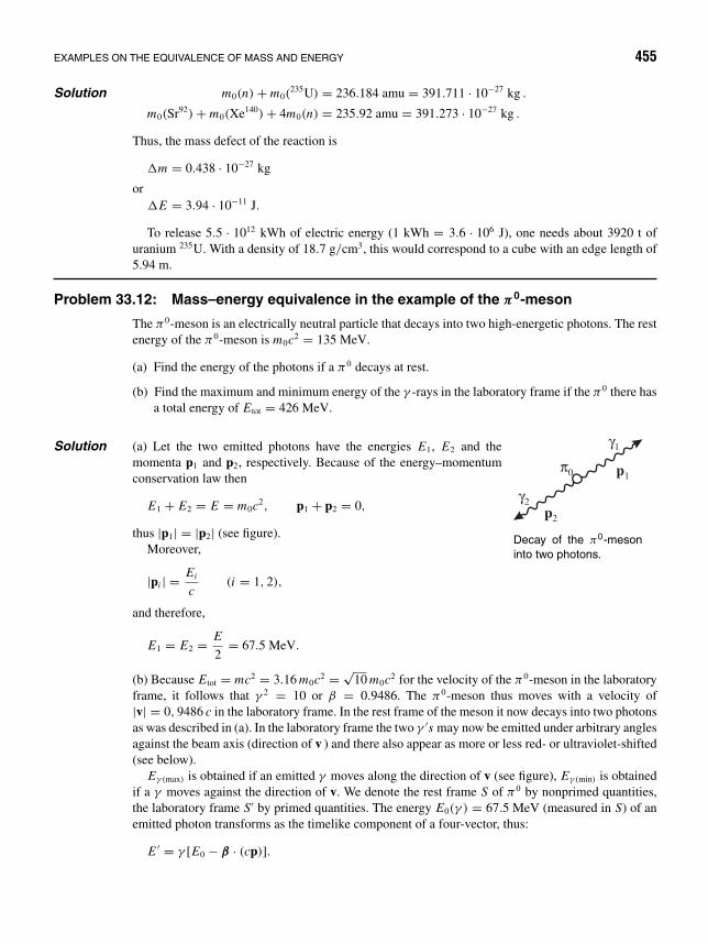
EXAMPLES ON THE EQUIVALENCE OF MASS AND ENERGY 455
Solution m0(n) + m0(235U) = 236.184 amu = 391.711 · 10−27 kg .
m0(Sr92) + m0(Xe140) + 4m0(n) = 235.92 amu = 391.273 · 10−27 kg .
Thus, the mass defect of the reaction is
m = 0.438 · 10−27 kg
orE = 3.94 · 10−11 J.
To release 5.5 · 1012 kWh of electric energy (1 kWh = 3.6 · 106 J), one needs about 3920 t ofuranium 235U. With a density of 18.7 g/cm3, this would correspond to a cube with an edge length of5.94 m.
Problem 33.12: Mass–energy equivalence in the example of the π0-meson
The π 0-meson is an electrically neutral particle that decays into two high-energetic photons. The restenergy of the π0-meson is m0c2 = 135 MeV.
(a) Find the energy of the photons if a π0 decays at rest.
(b) Find the maximum and minimum energy of the γ -rays in the laboratory frame if the π0 there hasa total energy of Etot = 426 MeV.
γ1
p1
p2
γ2
π0
Decay of the π0-mesoninto two photons.
Solution (a) Let the two emitted photons have the energies E1, E2 and themomenta p1 and p2, respectively. Because of the energy–momentumconservation law then
E1 + E2 = E = m0c2, p1 + p2 = 0,
thus |p1| = |p2| (see figure).Moreover,
|pi | = Ei
c(i = 1, 2),
and therefore,
E1 = E2 = E
2= 67.5 MeV.
(b) Because Etot = mc2 = 3.16 m0c2 = √10 m0c2 for the velocity of the π0-meson in the laboratory
frame, it follows that γ 2 = 10 or β = 0.9486. The π0-meson thus moves with a velocity of|v| = 0, 9486 c in the laboratory frame. In the rest frame of the meson it now decays into two photonsas was described in (a). In the laboratory frame the two γ ′s may now be emitted under arbitrary anglesagainst the beam axis (direction of v ) and there also appear as more or less red- or ultraviolet-shifted(see below).
Eγ (max) is obtained if an emitted γ moves along the direction of v (see figure), Eγ (min) is obtainedif a γ moves against the direction of v. We denote the rest frame S of π 0 by nonprimed quantities,the laboratory frame S′ by primed quantities. The energy E0(γ ) = 67.5 MeV (measured in S) of anemitted photon transforms as the timelike component of a four-vector, thus:
E ′ = γ [E0 − β · (cp)].

456 THE BASIC QUANTITIES OF MECHANICS IN MINKOWSKI SPACE 33
γ1
p1
p2
m0γ2
vπ0,Etot
vπ0
or
Eγ(min) Eγ(max)
The situation before (left) and after (right) the decay of the π0-meson.
In S one has |p| = E0/c, and the maximum (minimum) γ -energy is obtained if p points in negative(positive) β-direction (as seen from the S-frame). Hence:
Eγ (max) = γ · E0(1 + β) =√
1 + β
1 − β· E0 = 416 MeV,
and
Eγ (min) = γ · E0(1 − β) =√
1 − β
1 + β· E0 = 10.9 MeV.
Problem 33.13: On pair annihilation
Let an isolated system contain 6 · 1027 protons and the same number of antiprotons at rest. (m0(p) =m0(p) = 1.7 ·10−27 kg.) Let all protons and antiprotons annihilate each other and produce 30 ·1027π -mesons. What is the mean kinetic energy of the π -mesons? (m0(π)/m0(p) = 0.15.)
Solution The total mass of the system is Mtotal = 12 · 1027 m(p). Because 30 · 1027π -mesons are created,each of them on the average has a total energy of m total(π) = 12
30 m0(p) = 0.4 m0(p). From thereimmediately follows a mean kinetic energy of
Ekin(π) = [m total(π) − m0(π)]c2 =[
0.4 − m0(π)
m0(p)
]mpc2
= (0.4 − 0.15) · 0.937 GeV = 234 MeV.
Problem 33.14: Kinetic energy of the photon
L
Sour ce
Photon Source
Detector Detector
ν
ν
ν ν ν>
Emission and detection of photons inthe gravitational field of the earth.
A certain radioactive nucleus emits photons of energyE = h and momentum p = h/c. A precision tech-nique based on the “Mossbauer effect” allows frequencymeasurements up to an accuracy of d/ = 10−15. Thephotons of frequency are absorbed by a detector. If theemitter and the detector are at equal altitude above theearth’s surface, the detector receives a photon of frequency′ = . This is no longer true if the emitter is at an altitudeL above the detector (see figure).
(a) The rest mass of a photon is m0 = 0. What is theactual mass of a photon of energy E = h?
(b) If a photon falls through an altitude L in the earth’sgravitational field, then its potential energy decreases.

EXAMPLES ON THE EQUIVALENCE OF MASS AND ENERGY 457
As a result, the photon gains “kinetic” energy. How large is the photon energy E ′ when the photonhits the detector?
(c) What frequency ′ is measured by the detector?
(d) Assume that the photon falls from an altitude L = 10 m. Could one measure the frequency shiftin the gravitational field of earth by means of the Mossbauer effect?
(e) Could this effect have a bearing on the light emission of very heavy stars?
Solution (a) Because E = h = mc2, it follows for the mass of a photon that
m = h
c2.
(b) The potential energy of a photon of mass m at the altitude L above ground follows from
d E
dx= mg = E
c2g
by integration; thus
E ′ = E egl/c2 ≈ E
(1 + gL
c2
)= h
(1 + gL
c2
).
If the photon “falls down” by the altitude L , it gains this energy according to
E ′ = E + mgL =(
1 + gL
c2
)h.
(c) The new frequency immediately results from there as
′ =(
1 + gL
c2
).
(d) As a relative frequency shift, we consider the quantity
= gL
c2= 10−15, for L = 10 m.
That is, with a fall distance of 10 m on earth, the effect is measurable by means of the Mossbauereffect. The experiment was performed first in 1960 by Pound13 and Rebka with a fall distance of 72ft (about 22 m). They obtained an experimental value of (5.13 ± 0.51) · 10−15 as compared with thetheoretical prediction of 4.92 · 10−15.
(e) If light leaves the gravitational field of the emitting body, it gains potential energy and thereforeappears as red-shifted. We therefore see very heavy stars “colder” than they actually are at theirsurface.
13Robert Vivian Pound, b. 1919, Ridgeway, Ontario, Canada. He held research positions at MIT from 1942–1946, and at Harvard from 1946–1989. Pound did pioneering work in the areas of nuclear magnetic resonance(NMR), radar, and experimental tests of Einstein’s general theory of relativity. The experiment of “weightingphotons” was done in collaboration with his graduate student Glen Rebka.

458 THE BASIC QUANTITIES OF MECHANICS IN MINKOWSKI SPACE 33
Problem 33.15: The so-called twin paradox
On the earth are living triplets A, B, and C . At earth time t = 0, B and C each board a spaceshipand go away from earth on straight lines. A observes the travels of the brothers from the earth andrealizes the following by his clocks and scales: B for one year experiences a uniform acceleration,such that he comes from velocity zero to a velocity of v = 0.8 c. He then flies for another year withthis constant velocity. During a further year B reduces his velocity and reverses it to −0.8 c. He againflies for one year with this velocity, and in the course of a further year he reduces his velocity to zeroto land again on earth. C makes a similar trip as B, during which he, as stated by A, in one yearuniformly accelerates to a velocity of 0.8 c, but then flies 11 years with this velocity, within a furtheryear returns in the same way as B, with constant velocity flies back 11 years, and then reduces hisvelocity during one year to zero and lands again at A on earth. Let B and C have determined theduration of their trip with the same kinds of clocks as A did.
(a) Sketch the states of motion of the three brothers in a space-time (t, x) diagram.
(b) The two brothers B and C compare the duration of their trips after the landing of C on earth.What difference exists between the duration of C’s trip determined by C’s clock and the durationof B’s trip determined by B’s clock?
(c) For the observer A on earth, the time difference between the duration of C’s trip and that of Bamounted to 20 years. Compare this statement with the result from (b). Doesn’t this lead to acontradiction to the postulate of relativity of the special theory of relativity, which states that allinertial frames are on equal rights?
(d) Let us assume that a further observer D at the moment t = 0 was accelerated instantaneously toits velocity v = 0.8 c. According to A on earth, D moves away from earth for 10 years with thisconstant velocity; then he instantaneously turns his velocity around by a strong acceleration andflies back to earth with v = 0.8 c. After 10 more years of flight with constant speed, he againreaches the earth, where he instantaneously reduces his speed to zero and lands at A. We shallassume that the number of heartbeats of A and D measures their corresponding proper time thathas passed. How does the space-time diagram of A and D look like? How much did A and D ageduring the flight of D?
Solution (a) In the space-time diagram, the motions of A, B, and C look as plotted in the figure:
25
20
15
10
5
0
t (years)
x
A C
B
Space-time map of the journeys of the triplets A, B, and C.

EXAMPLES ON THE EQUIVALENCE OF MASS AND ENERGY 459
(b) Since B and C have passed acceleration periods, we cannot calculate the proper times τB andτC of the trips of B and C , respectively. However, the acceleration periods for B and C were identical,hence we may calculate the difference of the proper times τC − τB by considering only the intervalsof constant velocity. As seen from earth these are for the motion of B in total 2 years, for C in total22 years. B and C flew during these periods with the same velocity of v = 0.8 c relative to earth. Wethen may calculate τ ≡ τC − τB by means of the time dilatation factor:
t = 20 y = γτ
or
τ = γ −1 · 20 y =√
1 − 0.82 · 20 y = 12 years.
Thus, if B and C compare the trip durations measured by their own clocks, they realize that C was12 years longer on the way than B. If they directly compare the display of their clocks, it turns outthat C’s clock shows 8 years less than the clock of B, who after his return to earth still had to wait 20earth years for C’s return.
(c) Although after landing of C on earth all three brothers may compare their clocks at one positionon earth, the time difference of the trips of C and B according to their statements amounts to 12years, although A states 20 years for that. One might now argue as follows: During the phases ofconstant speed A moves with a speed of |v| = 0.8 c relative to B or C , such that both B and C seethe time evolutions at A slowed down. For reasons of symmetry the relativity principle should thenimply that the above difference on their statements was not permissible. This reasoning is, however,wrong. There is no symmetry between the motion of A and the motion of B or C , because the latterboth were accelerated (absolutely) and thus did not always stay in an inertial frame.
(d) The space-time diagram of A and D looks as follows:
20
15
10
5
0
t (years)
x
AD
Space-time map of the journey of voyager D.
During the flight of D 20 years of proper time passed for A, while D ages by only τD =t · γ −1 = 12 years. Thus D aged by 8 years less than A did. The proper time that passed betweentwo space-time points x and y thus depends on the trajectory T of the observer between x and y. Itis given by the arc length τ(T ) = 1
c
∫ yx ds of the trajectory between x and y. That in our example
τD < τA, although the world line of D in the above figure is larger than that of A, is a consequenceof the indefinite metric of the space-time continuum.

460 THE BASIC QUANTITIES OF MECHANICS IN MINKOWSKI SPACE 33
Problem 33.16: Kinetic energy of a relativistic particle
The kinetic energy of a nonrelativistic particle reads
T = 1
2m0v2 = p2
2m0,
where p = m0v is the momentum of the particle. Find a formally similar expression for the relativistickinetic energy.
Solution One has
E = mc2 = m0c2√1 − v2/c2
(33.73)
for the relativistic total energy of a free particle and
p = mv = m0v√1 − v2/c2
(33.74)
for the relativistic momentum. According to (33.59) for (33.73) the following form still exists:
E2 = c2p2 + (m0c2
)2
= c2p2 + E20 , (33.75)
with E0 = m0c2 the rest energy. Hence
c2p2 = E2 − E20 = (E − E0)(E + E0),
and therefore it follows for the relativistic kinetic energy that
T = E − E0 = c2p2
(E + E0)= c2p2
(m + m0)c2
= p2
m + m0. (33.76)
This is the desired form. Obviously one has
limv→0
T = p2
m0 + m0= p2
2m0(33.77)
and
T = m2v2
m0
(1 + 1/
√1 − v2/c2
) = m2√
1 − v2/c2 v2
m0
(1 +√
1 − v2/c2)
= mv2
1 +√1 − v2/c2
=︸︷︷︸v→c
mv2 = p · v.
These relations were pointed out first by W.G. Holladay (Vanderbilt University, Nashville, Ten-nessee.).

34 Applications ofthe SpecialTheory ofRelativity
The elastic collision
In the general collision problem we are interested in the changes of momenta and energiesof the colliding particles. The only assumption about the interaction adopted here is that itshall act only at very small distances between the particles. The problem may be solved bymeans of the conservation laws of momentum and energy. We denote the four-momenta of
the two particles before the collision by⇒p and
⇒P , and after the collision by
⇒p′ and
⇒P ′. The
four-momentum conservation law then reads⇒p + ⇒
P=⇒p′ +
⇒P ′ . (34.1)
The four-vector equation comprises two conservation laws, namely that for the usualthree-momentum
p + P = p′ + P′ (34.2)
(see equation (33.57)), and that for the energy
e + E = e′ + E ′ = E, (34.3)
where with the rest masses of the particles m0 and M0
e2
c2= m2
0c2 + p2,E2
c2= M2
0 c2 + P2 (34.4)
461

462 APPLICATIONS OF THE SPECIAL THEORY OF RELATIVITY 34
are the energies of the particles before the collision. Because the collision was supposed aselastic, the rest masses m0 and M0 remain unchanged in the collision process. Therefore,the energies of the particles after the collision are given by e′ and E ′, where
e′2
c2= m2
0c2 + p′2,E ′2
c2= M2
0 c2 + P′2. (34.5)
The total energy of the considered system has been denoted by E . In (34.2) and (34.3), therest masses and the components of the initial momenta are to be considered as given. We arelooking for the components of the final momenta p′ and P′. Hence, we have four equationsfor six unknown quantities, such that the general solution will contain two undeterminedparameters.
The collision problem becomes most simple in that coordinate frame where the initialmomenta p and P are oppositely equal. This is the frame in which the total momentumvanishes and therefore the center of mass of the two particles is at rest. This is the rest frameof the center of mass, which is often denoted more briefly as the center-of-mass system.In this frame because of (34.1) also the final values p′ and P′ of the momenta must beoppositely equal.
αp
p´
P´
P
The elastic collision in the center-of-mass system.
On the other hand, the energy law (34.3) requiresthat the magnitudes |p| = |P| and |p′| = |P′| of themomenta remain unchanged in the collision:
|p| = |p′|or simply
p = p′, (34.6)
with the abbreviations p = |p|, P = |P′|, etc. In thecollision process only the straight line along the initialdirection of the two momenta is arbitrarily rotated inspace (see figure).
The deflection angle α represents one of the unde-fined parameters. The second parameter is the azimuthangle specifying the position of the plane defined by p and p′, which evidently may bearbitrarily rotated about the direction of p.
Of particular interest for physical applications is the case with one of the particles, forexample, the second one, being at rest before the collision:
P = 0. (34.7)
Formula (34.2) then simplifies to
p = p′ + P′. (34.8)
The energy equation retains its form (34.3), but now from (34.4) it follows that
E
c= M0c. (34.9)

THE ELASTIC COLLISION 463
αθpp´
P´
Momentum balance of a colliding par-ticle and a particle at rest.
In this case one may choose the angle θ or α as thefirst undetermined parameter (figure). The second pa-rameter is again the azimuth angle, which determinesthe position of the drawing plane of the figure thatmay be arbitrarily rotated about the direction of p; ithas no meaning for the following calculation.
The solution of this particular collision problemmight be found from the solution in the center-of-masssystem by Lorentz-transforming to the rest frame ofthe second particle. Here we shall derive the final formula from (34.8), (34.3), and (34.9)by straightforward calculation.
We choose the angle θ as parameter and write down the trigonometric formula thatfollows immediately from the figure (see also equation (34.8))
P ′2 = p′2 + p2 − 2p p′ cos θ. (34.10)
By forming the square of the relation following from (34.5) and (34.3) (ε = E/c)
ε −√
M20 c2 + P ′2 =
√m2
0c2 + p′2 ,
there results
p′2 + m20c2 = P ′2 + M2
0 c2 + ε2 − 2ε
√M2
0 c2 + P ′2 .
When inserting in this relation the value (34.10) of P ′2, the resulting equation containsbesides the term with the square root only a part linear in p′. Thus, one may eliminate thesquare root by one more squaring and obtain an equation of second degree in p′:
(m20c2 − M2
0 c2 − p2 − ε2 + 2p p′ cos θ)2 − 4ε2(M20 c2 + p2 + p′2 − 2p p′ cos θ) = 0 .
By explicitly calculating the square and rearranging the terms, one gets
4(
p2 cos θ − ε2)
p′2 + 4p p′ cos θ(m2
0c2 − M20 c2 − p2 + ε2
)(34.11)
+ (m2
0c2 − M20 c2
)2 − 2(
p2 + ε2)
m20c2 + (
ε2 − p2)
M20 c2 + (
p2 − ε2)2 = 0 .
This equation can be brought to a simpler form by making use of the relations
ε =√
p2 + m20c2 + M0c, (34.12)
ε = e
c+ M0c (34.13)

464 APPLICATIONS OF THE SPECIAL THEORY OF RELATIVITY 34
which follow from (34.3), (34.4), and (34.7). By inserting (34.13) in the first summand of(34.11) and (34.12) in the second and third summands, a further muliplication by −1/4yields((e
c+ M0c
)2 − p2 cos θ
)p′2 (34.14)
− 2pp′ cos θ
(m2
0c2 + M0c√
p2 + m20c2
)− p2c2
(M2
0 − m20
) = 0 .
In the second summand, one now replaces√
p2 + m20c2 by e/c according to (34.4), and
finally one ends up with a quadratic equation for p′:((e
c+ M0c
)2 − p2 cos θ
)p′2 (34.15)
− 2pp′ cos θ(
m20c2 + M0c
e
c
)− p2c2
(M2
0 − m20
) = 0 .
Solving for p′ yields the final result
p′ = p
(M0c + e/c)2 − p2 cos2 θ
cos θ
(m2
0c2 + M0ce
c
)±(e
cc + M0c2
)√M2
0 − m20 sin2 θ
. (34.16)
We still note that for M0 > m0 only the positive sign before the square root in (34.16)must be admitted. According to (34.12), ε > p and therefore ε2 − p2 cos2 θ > 0. Theexplanation for this behavior is provided by (34.16). In the case M0 < m0, the angle θ
passes twice through the range 0 ≤ θ ≤ θmax, whereby θmax follows from
M0 = m0 sin θmax.
Therefore to any angle θ in this range will correspond two solutions of the collision problem.In the case M0 > m0, however, θ passes the range 0 ≤ θ ≤ π once, hence for any value ofθ there is only one solution.
By inserting the value (34.16) of p′ in the first of equations (34.5), there results after anelementary calculation the value of e′/c. The final formula reads
e′
c= 1
(M0c + e/c)2 − p2 cos2 θ
(e
c+ M0c
) (M0c
e
c+ m2
0c2)
± cp2 cos θ
√M2
0 − m20 sin2 θ
. (34.17)
To finish the calculation, we still have to give formulas for P′ and E ′/c. P′ may becalulated immediately from (34.7), namely
P′ = p − p′, (34.18)

COMPTON SCATTERING 465
since p′ is determined by p′ and the angle θ . The energy E ′/c is most simply calculatedfrom (34.3) and (34.9):
E ′
c= M0c + e
c− e′
c. (34.19)
The formulas (34.16) to (34.19) represent the complete solution of the given collisionproblem.
Compton scattering
We will apply these formulas to the case of the collision of a photon with an electron atrest. The special feature of the photon is that its rest mass is extremely small against the restmass of the electron and possibly even strictly equals zero. This simplifies considerably thealgebra we had needed in the previous section.
In the course on quantum mechanics, we will see in detail how the photon energy e isrelated to the frequency and the wavelength λ of the radiation. We will find
e = hω = h = hc · 2π
λ= hc
λ. (34.20)
Here h = h/2π is the Planck quantum of action (h = 1.054571 × 10⁻³⁴ Js), and ω = 2πis the angular frequency of the photon oscillation. The momentum of the photon is given by
p = hk (34.21)
which defines the so-called wave vector k of the photon.When photons of X-rays are scattered by electrons, a frequency shift can be observed,
the amount of this shift depending on the scattering angle. This effect was discoveredby Compton in 1923 and explained on the basis of the photon picture simultanously byCompton himself and Debye.
αθpp´
P´
Conservation of momentum in Comp-ton scattering.
The figure illustrates again the kinematical situa-tion. We assume the electron is unbound and at restbefore the collision. Then the conservation of energyand momentum reads
hω + m0c2 = hω′ + m0c2√1 − β2
, (34.22)
hk = hk′ + m0v√1 − β2
(34.23)
To obtain a relation between the scattering angle θ and the frequency shift, we split up(34.23) into components parallel and vertical to the direction of incidence. This yields, withk = ω/c,
hω
c= hω′
ccos θ + m0v√
1 − β2cos α (34.24)

466 APPLICATIONS OF THE SPECIAL THEORY OF RELATIVITY 34
andhω′
csin θ = + m0v√
1 − β2sin α . (34.25)
From these two component equations, we can first eliminate α and then, by (34.22), theelectron velocity v (β = v/c). To this end, we bring the cos θ term from equation (34.24)to the left hand side, sqare and add the square of equation (34.25):(
hω
c− hω′
ccos θ
)2
+(
hω′
csin θ
)2
=(
m0v√1 − β2
)2 (cos2 α + sin2 α
)(34.26)
or (hω
c
)2
− 2hω
c
hω′
ccos θ +
(hω′
c
)2
=(
m0v√1 − β2
)2
= m20v
2
1 − v
c2
. (34.27)
From (34.22) we get
(hω − hω′ + m0c2
)2 =(m0c2
)2
1 − v2
c2
, (34.28)
or
1 − v2
c2=
(m0c2
)2(hω − hω′ + m0c2
)2 , v2 = c2
(1 −
(m0c2
)2(hω − hω′ + m0c2
)2
). (34.29)
Hence,
m20v
2
1 − v
c2
= m20c2
(1 −
(m0c2
)2(hω − hω′ + m0c2
)2
)·(hω − hω′ + m0c2
)2(m0c2
)2
= m20c2
((hω − hω′ + m0c2
)2(m0c2
)2 − 1
)T
= 1
c2
((hω − hω′ + m0c2
)2 − (m0c2
)2)
= 1
c2
((hω − hω′)2 + 2
(hω − hω′)m0c2
)=(
hω
c
)2
+(
hω′
c
)2
− 2hω
c
hω′
c+ 2h
(ω − ω′)m0 .
Inserting this in (34.23), we obtain
2hω
c
hω′
c(1 − cos θ) = 2h
(ω − ω′)m0 . (34.30)

COMPTON SCATTERING 467
Using the trigonometric identity
1 − cos θ = 2 sin2 θ
2, (34.31)
we finally obtain the following result for the frequency difference:
ω − ω′ = 2h
m0c2ωω′ sin2 θ
2. (34.32)
If we put ω = 2πc/λ, we obtain the Compton scattering formula in the usual form withthe difference in wavelength as a function of the scattering angle θ ,
λ′ − λ = 4πh
m0csin2 θ
2= 2λc sin2 θ
2. (34.33)
The scattering formula shows that the change in wavelength depends only on the scatteringangle θ . During the collision the photon loses a part of its energy, and the wavelengthincreases (λ′ > λ).
The factor 2πh/m0c is called the Compton wavelength λc of a particle with rest massm0 (here, an electron). The Compton wavelength can be used as a measure of the size of aparticle. The electron has the Compton wavelength λc = 2.426 × 10⁻¹² m.
The kinetic energy of the scattered electron is
T = hω − hω′ = h2πc
(1
λ− 1
λ′
), (34.34)
0o
15o
30o
45o
45o
60o
60o
75o
75o
90o
90o
105o
105o
120o
120o
135o
135o
150o
150o
165o
165o
180o 180
o
photon energy
electron energy
The Compton effect energy distribution of photons and electrons, showing the dependence on the scat-tering angle. The total available photon energy is the dashed grey line, corresponding to no scatteringof the photon, θ = 0.

468 APPLICATIONS OF THE SPECIAL THEORY OF RELATIVITY 34
or, using
1
λ− 1
λ′ = λ′ − λ
λ′λ= 1
λ
2λC sin2 θ2
λ + 2λC sin2 θ2
(34.35)
and, again with 2πc/λ = ω,
T = hω2λC sin2 θ
2
λ + 2λC sin2 θ2
. (34.36)
Thus the energy of the scattered electron is directly proportional to the energy of the photon.Therefore the Compton effect can only be observed in the domain of short wavelengths,such as X-rays and γ -rays. To appreciate this observation fully, we mention that in classicalelectrodynamics, no alteration in frequency is permitted in the scattering of electromagneticwaves – this change in frequency is only possible if scattering occurs at light quantawith momentum p = hk end energy e = hω. Thus the idea of light quanta has beenexperimentally confirmed by the Compton effect.
The inelastic collision
In an inelastic collision, kinetic energy is lost. By definition, also the rest masses of both orat least one of the colliding particles are changing. In this case the values of the rest massesbefore the collision shall be denoted by m0 and M0, the values after the collision by m ′
0 andM ′
0. Equations (34.1), (34.4), and (34.2, 34.3) hold also here without any modification. Onthe contrary, (34.5) changes to(
e′
c
)2
= m ′20 c2 + p′2,
(E ′
c
)2
= M ′20 c2 + P ′2. (34.37)
We still note that according to the adopted definition the inelastic collision must notnecessarily be connected with a loss of kinetic energy. Kinetic energy is consumed onlythen if the sum of the rest masses is increased by the collision process, namely, if m ′
0+M ′0 >
m0 + M0. In the case m ′0 + M ′
0 < m0 + M0, on the contrary, kinetic energy is created.The formulas (34.1), (34.4), (34.2), (34.3), and (34.37) may also then be applied if
the two colliding particles disappear and two new particles are produced in the collisionprocess. m ′
0 and M ′0 then represent the rest masses of the new arising particles. Such a
case is the annihilation of an electron-positron pair, where m0 = M0 = rest mass of theelectron (positron) and m ′
0 = M ′0 = rest mass of the photon = 0. We consider this process
in the center-of-mass system of the electron-positron pair. Then p = −P. Therefore,according to the momentum conservation law (34.2), also p′ = −P′, that is, the twophotons are emitted in opposite directions with equal momenta, hence also equal energies(figure). The relation between p and p′ follows from the energy conservation law. Because
e/c = E/c =√
m20c2 + p2 and e′/c = E ′/c = p′, from (34.3) we get
p′ =√
m20c2 + p2. (34.38)

THE INELASTIC COLLISION 469
According to (34.20), the energy of every photon is
h = cp′ =√
m20c4 + p2c2. (34.39)
The smallest photon energy therefore corresponds to the case p = 0 and is equal to therest energy m0c2 of the electron.
p
p´
P´
P
Momentum balance of a binary collisionin the center-of-mass frame.
The inverse process of annihilation—the creationof an electron-positron pair—occurs in the interac-tion of a sufficiently energetic photon with an atomicnucleus. This is a process that differs from the col-lision considered so far. Before the interaction twoparticles are present also here: the photon and theatomic nucleus. After the collision, however, threeparticles are involved: the atomic nucleus and theelectron-positron pair. The most important featureof this process, which is significant for the experi-mental verification of the theorem on the inertia ofenergy, can however be derived immediately fromthe energy conservation law.
If we denote the photon energy by hω, the rest mass of the atomic nucleus and theelectron (positron) by M0 and m0, and the final values of the momenta of the three particlesby P, p−, and p+, we have
hω + M0c2 =√
M20 c4 + P2c2 +
√m2
0c4 + p2−c2 +√
m20c4 + p2+c2. (34.40)
Here we assumed that the atomic nucleus was at rest before the interaction. From thisrelation follows immediately
hω > 2m0c2. (34.41)
This means that the process is possible only with photons of an energy exceeding the sum ofthe rest energies of two electrons. This has been explained already in the preceding chapter.
As another example of inelastic collisions we mention the nuclear reactions. If therebyonly two particles are present also after the collision then the process is again described byequations (34.1), (34.4), (34.2), (34.3), and (34.37). But in this case the energy equationmay be simplified since, as a rule, the velocities of all particles are small against the speedof light. For such particles, which are usually denoted as nonrelativistic, there holds to goodapproximation the relation following from (34.4) and (33.34):
e = m0c2 + 1
2m0q2.
Therefore, the energy law (34.3) reduces to
(m0 + M0)c2 + Ekin = (m ′
0 + M ′0)c
2 + E ′kin. (34.42)

470 APPLICATIONS OF THE SPECIAL THEORY OF RELATIVITY 34
Here Ekin and E ′kin denote the sum of the kinetic energies before and after the collision
calculated by means of (33.34). When denoting the velocities of the particles before andafter the collision by q, Q and q ′, Q′, respectively, this means
Ekin = 1
2m0q2 + 1
2M0 Q2, E ′
kin = 1
2m ′
0q ′2 + 1
2M ′
0 Q′2. (34.43)
Decay of an unstable particle
The most simple case is obviously that the unstable particle decays into two new particles.The most important results may also be derived here from the conservation laws. For sakeof simplicity we consider the process in the rest frame of the original particle. From themomentum conservation then follows that the momenta p′ and p′′ of the two new particlesmust sum up to zero,
p′ = −p′′. (34.44)
When denoting the rest mass of the original particle by M0, and the rest masses of thenew particles by m ′
0, m ′′0, the energy conservation law reads
M0c =√
m ′20 c2 + p′2 +
√m ′′2
0 c2 + p′2. (34.45)
We thereby have taken into account the relation p′′ = p′ following from (34.44). If therest masses M0, m ′
0 and m ′′0 are known, one may determine the value of p′ from (34.45). In
this decay mode thus in the decay of particles at rest the new particles are always emittedwith the momentum p′ following from (34.45), and therefore with the uniquely definedenergy values
e′ =√
m ′20 c4 + p′2c2, e′′ =
√m ′′2
0 c4 + p′2c2. (34.46)
The decay into more than two new particles may also be treated in a similar way. If onedeals, for example, with a decay into three new particles, the conservation laws in the restframe of the original particle read
0 = p′ + p′′ + p′′′, (34.47)
M0c =√
m ′20 c2 + p′2 +
√m ′′2
0 c2 + p′′2 +√
m ′′′20 c2 + p′′′2. (34.48)
We shall not discuss these equations in detail but mention only an important qualitativeconclusion. Contrary to the preceding case, the momentum equation now can no longer re-duce the momentum values arising after the decay p′, p′′, p′′′ to a single quantity. Therefore,from the energy equation determined values of these quantities no longer follow uniquely.In a decay with more than two product particles, the new particles are no longer—as inthe case of two product particles—emitted with uniquely determined energy values but

DECAY OF AN UNSTABLE PARTICLE 471
shall show a continuous energy spectrum. This fact, by the way, led W. Pauli1 in 1930 topostulate the neutrino as a hypothetical decay product in the β-decay of the neutron.2 Lateron these particles were actually experimentally detected.
Problem 34.1: The relativistic rocket
If rockets reach velocity ranges comparable to the speed of light, the equations of motions mustbe based on relativistic mechanics. Formulate the general equation of motion for this problem anddiscuss it for the one-dimensional case.
Solution We denote by pµ the four-momentum of the spaceship, and by dqµ = δm ·ωµ the four-momentum ofthe mass δm expelled by the ship per unit time, as seen from an inertial frame. Energy conservationrequires
pµ = dqµ + (pµ + dpµ) (34.49)
with the new four-momentum of the ship pµ + dpµ. We insert dqµ and dpµ = d(muµ) and divideby the proper time dτ :
0 = δm
dτωµ + dm
dτuµ + m
duµ
dτ. (34.50)
δm/dτ und dm/dτ are the rates for the expelled masses and for the related decreasing mass of theship. The relation δm/dτ = −dm/dτ now no longer holds! We define λ = δm/dτ :
muµ + muµ = −λωµ. (34.51)
We multiply (34.51) by uµ and employ uµuµ = −c2 and uµuµ = 0 (here the Einstein sumconvention is used, which means an automatic sum over pairs of equal indices), because
d
dτ(uµuµ) = uµuµ + uµuµ = 0.
1Wolfgang Pauli, Swiss physicist of Austrian descent, b. April 25, 1900, Vienna—d. Dec. 15, 1958, Zurich.Pauli was a student of Arnold Sommerfeld in Munich, where he also became acquainted with Werner Heisenberg.At a student in his third year, he wrote a review article on the theory of relativity for the Enzyklopadie dermathematischen Wissenschaften. With his doctoral thesis from 1921 he for the first time cast doubt on the then-prevailing quantum theory (model of the atom of Bohr and Sommerfeld). His discussions with Heisenberg, MaxBorn, and Niels Bohr did contribute eminently to the development of matrix mechanics, the algebraic formulationof quantum mechanics. In 1926 he successfully applied the new theory on the hydrogen atom. Already in 1924he had discovered the exclusion principle (Pauli priciple), for which he was honored with the 1945 Nobel Price(awarded in 1946). Also in 1924 Pauli postulated the existence of the spin of the atomic nucleus in oder toexplain the hyperfine structure of atomic spectra. In 1927 he formulated a field equation for the electron, takinginto account the spin in a non-relativistic manner. Pauli was a professor in Hamburg from 1926–1928, and atETH Zurich from 1928 on. In 1930, he formulated the neutrino hypothesis, which was later on corroboratedby experiment. From 1940–1945, he stayed in the United States, working mainly on the theory of mesons. Hislater works back in Zurich in 1946 centered mainly around particle physics and the quantum theory of fields.Pauli made a lasting impression on modern physics and its way of thinking. With his profound analysis of theepistemological foundations of this science and his harsh criticism of obscure thinking, he was known as the“conscience of physics.”
2see e. g. W. Greiner and B. Muller, Gauge Theories of Weak Interactions, Springer Verlag New York, 2000

472 APPLICATIONS OF THE SPECIAL THEORY OF RELATIVITY 34
From there it follows that
λ = mc2
uµωµ. (34.52)
Hence we have the equation of motion of a body with variable mass, as is represented by therocket.
d
dτ(muµ) = − mc2
uωωµ. (34.53)
Solving this equation for a one-dimensional problem causes no trouble. We write for the twovelocities ω and u
ω
c≡ tanh φ,
u
c≡ tanh θ, (34.54)
and using h = c tan α and α = θ − φ we may express the velocity of the expelled matter relative tothe ship.
uωµ = c2(sinh θ sinh φ − cosh θ cosh φ) = −c2 cosh(θ − φ) = −c2 cosh α. (34.55)
Equation (34.53) for µ = 1 then takes the following form:
d
dτ(m c sinh θ) = mc2
c2 cosh αc sinh φ, (34.56)
and finally reduces to the simple differential equation
m sinh θ + mθ cosh θ = msinh φ
cosh α,
m sinh θ cosh α + mθ cosh θ cosh α = m sinh φ,
m(sinh θ cosh α − sinh φ) + mθ cosh θ cosh α = 0,
m sinh α + mθ cosh α = 0
⇒ mθ + mh
c= 0. (34.57)
Here we have made use of the relation
sinh φ = sinh(θ − α) = sinh θ cosh α − cosh θ sinh α .
If with h the relative expulsion velocity of the mass is constant, θ may be given as a function of themass:
θ = log( m
M
)−h/c. (34.58)
M is the integration constant, which here plays the role of the start mass of the spaceship.
u
c= tanh θ = 1 − e−2θ
1 + e−2θ= 1 − (m/M)2h/c
1 − (m/M)2h/c.
If we assume that the relative expulsion velocity of the expelled mass is about h ≈ c and half ofthe start mass is released, then the final velocity is
u
c= 1 − (0.5)2
1 + (0.5)2= 3
5.

DECAY OF AN UNSTABLE PARTICLE 473
Problem 34.2: The photon rocket
The emission of electromagnetic radiation is considered as an option for driving spaceships in future.Start from the equation (34.51) of the problem of the relativistic rocket and compare the two
propulsion systems.
Solution The equation of motion reads
d
dτ(muµ) = −λPµ. (34.59)
Pµ is the four-momentum vector of the emitted radiation. We again multiply by uµ and get, usingagain the Einstein sum convention, which means an automatic sum over pairs of equal indices,
muµuµ + muµuµ = −λuµ Pµ (34.60)
⇒ λ = m2c2
uµ Pµbecause of uµuµ = −c2 and uµuµ = 0.
Thus, equation (34.59) reads
d
dτ(muµ) = −
(mc2
u P
)Pµ. (34.61)
We are already familiar with this result from the relativistic rocket. The difference is that the photonfour-momentum vector is a zero vector, because of the vanishing mass:
Pµ Pµ = 0. (34.62)
We again consider the one-dimensional case. Equation (34.62) then reduces to(P1)2 − (
P4)2 = 0 ⇔ P1 = ±P4. (34.63)
If the spaceship flies in positive x-direction, the photons necessarily should have a negativemomentum:
P1 = −P4. (34.64)
We now write down the discrete photon energy, using the de Broglie relation, thus
W = h ⇒ P4 = h
c, P1 = −h
c, (34.65)
u P = u1 P1 − u4 P4 = (u1 + u4
)P1 = − (
u1 + u4)
P4. (34.66)
Equation (34.61) for µ = 1 and µ = 4 then becomes(u1 + u4
) d
dτ
(mu1
) = −mc2, (34.67)
(u1 + u4
) d
dτ
(mu4
) = mc2. (34.68)
The sum of these two equations yields
d
dτ
(mu1 + mu4
) = 0 ⇒ mu1 + mu4 = Mc, (34.69)

474 APPLICATIONS OF THE SPECIAL THEORY OF RELATIVITY 34
where with M the start mass of the rocket was introduced via the integration constant; this is thesituation with u1 = 0 and u4 = c.
Rewriting again the equation by means of the definitions
u1 = c sinh θ u4 = c cosh θ (34.70)
there results
m(sinh θ + cosh θ) = M ⇔ m = Me−θ
⇒ u
c= tanh θ = 1 − (m/M)2
1 + (m/M)2. (34.71)
Thus, the final velocity does not depend on the frequency of the radiation. Nevertheless, it willpresumably take some time to overcome the enormous difficulties in developing photon engines.Such an engine should of course provide a sufficient thrust. We also don’t see an advantage of such atype of engine over engines emitting massive particles near the speed of light.
Problem 34.3: The relativistic central force problem
Solve the central force problem relativistically for a particle of mass m with the charge q and a centralcharge Q that is tightly fixed to the origin of the coordinate frame. You should take into considerationonly the electrostatic interaction K = (Qq/r 2) er .
Solution The relativistic form of the second Newtonian axiom is the four-vector equation
Fµ = m0d
dτuµ, (34.72)
with Fµ being the four-force (33.8), p. 429, and uµ the four-velocity (33.3):
Fµ =(γ K, iγ
vc
· K)
, (34.73)
uµ = (γ v, iγ c) , γ = 1√1 − v2
c2
. (34.74)
K and u are the force and velocity according to Newtonian mechanics, respectively. The expressionused here for the fourth component F4 of the four-force Fµ,
F4 = iγvc
· K = iγ
c
d
dtmc2,
follows immediately from (??), which states
d
dtmc2 = v · K .
But we must use as the only force K in the relativistic expression only the Lorentz force acting ona charged particle. The other important interaction, the gravitation, cannot be treated without furtherado in this calculus, since it depends on the masses involved. These problems will be treated in thegeneral theory of relativity. Our central force problem is based on the electrostatic interaction of thetwo charges Q and q.
K = Qq
r 2er , (34.75)

DECAY OF AN UNSTABLE PARTICLE 475
⇒ Fµ =(
γQq
r 2er , iγ
r 2
vc
erQq
r 2u · er
). (34.76)
We shall use cylindrical coordinates for this problem. But we have to take into account the dependenceof the unit vectors on the time. To do this, we recall that the four-velocity uµ(µ = 1, 2, 3, 4) is thederivative of the world vector xµ = (x1, x2, x3, ict) with respect to proper time,
uµ = dxµ
dτ=(
1√1 − β2
dxdt
,ic√
1 − β2
)= (γ v, icγ ) ,
where γ = 1/√
1 − β2, β = v/c, and v = dx/dt the usual three-velocity. In cylindrical coordinates,we have
xµ = (rer , z, ict) ,
uµ = dxµ
dτ=(
d
dτ(rer ),
dz
dτ, ic
dt
dτ
)= ((rer )
•, z, icγ ) . (34.77)
Here, the dot • means the derivative with respact to proper time τ , thus
(. . .)• = d
dτ= 1√
1 − β2
d
dt.
In planar cylindrical coordiantes (z = 0), the world vector reduces to
xµ = (rer , 0, ict) ,
where r = rer and the unit vectors in radial and in ϕ-direction are
er = (cos ϕ, sin ϕ) ,
eϕ = (− sin ϕ, cos ϕ).
The four-velocity hence is
dxµ
dτ= ((rer )
•, 0, icγ ) = (rer + r er , 0, icγ ) .
Because
er = ϕeϕ , eϕ = −ϕer ,
we get
⇒u= dxµ
dτ= (
rer + r ϕeϕ, 0, icγ)
, (34.78)
d2xµ
dτ 2=(
rer + r er + r ϕeϕ + r ϕeϕ + r ϕeϕ, 0, icdγ
dτ
),
= ((r − r ϕ2
)er + (2r ϕ + r ϕ) eϕ, 0, icγ
). (34.79)
Newton’s equations in their relativistic four-form read
d
dτpµ = Fµ or m0
d
dτ
(dxµ
dτ
)= Fµ;

476 APPLICATIONS OF THE SPECIAL THEORY OF RELATIVITY 34
hence in our case here
m0
((r − r ϕ2
)er + (2r ϕ + r ϕ) eϕ, 0, icγ
) =(
γQq
r 2er , iγ
r 2
vc
erQq
r 2u · er
). (34.80)
Comparing the components of the four-vectors and taking into account that
γ v = rer + ϕeϕ , (34.81)
we end up with the three equations
γQq
r 2= m
(r − r φ2
), (34.82)
0 = m(2r φ + r φ
), (34.83)
1
c
r 2r = m
d
dτ(γ c) = mγ c. (34.84)
The dots always denote derivation with respect to the proper time τ .Equation (34.83) multiplied by r yields as in the nonrelativistic case the angular momentum
conservation:
m0
(2r r φ + r 2φ
) = m0d
dτ
(r 2φ
) ⇒ L ≡ m0r 2φ = constant. (34.85)
The equation (34.84) ensures the conservation of energy:
d
dτ
(m0γ c + 1
c
r
)= 0 ⇒ E = m0γ c2 + Qq
r= constant
⇔ γ = E
m0c2− Qq
m0c2r. (34.86)
Now we still wish to extract from (34.82) an equation of motion. For this purpose we employ thetwo conservation laws just obtained.(
E
m0c2− Qq
m0c2r
r 2= m0
(r − L2
m20r 3
). (34.87)
We introduce the variable s = 1/r and, as in the nonrelativistic Kepler problem, transform to adifferential equation for s(φ).
r = −r 2 ds
dφφ = − L
m0
ds
dφ, (34.88)
r = − L
m0
d2s
dφ2φ = − L2
m20
s2 d2s
dφ2(34.89)
⇒ 1
m0c2(E − Qq s)Qq s2 = − 1
m0
(L2 s2 d2s
dφ2+ L2 s3
)
s ′′ + s =(
cL
)2
s − E Qq
L2c2. (34.90)

DECAY OF AN UNSTABLE PARTICLE 477
We define the “angular frequency” 2 = 1 − (Qq/mLc)2 and thereby may at once give thesolution of this well-known differential equation:
1
r= s = − E Qq
m20 L2c22
+ A cos(φ). (34.91)
There are bound solutions to the problem if
q Q < 0 and A <E |Qq|
m20 L2c22
.
In equation 34.91 we already have used that we wish to start with φ = 0 at the perihelion. Since differs from 1, there is no closed path, but rather an orbital precession arises (perihelion motion).A closed orbit does only exist for q = 0 or Q = 0, hence if there is no force. This means thatthe relativistic Kepler problem always yields rosette orbits, which show perihelion motion. This isplausible if we recall our discussion in Chapters 26 and 28.
The constant A may be determined by inserting our solution in the following relation, which mustbe obeyed by the four-velocity uµ = (r , φ, 0, γ c) from equation 34.78:
⇒u · ⇒
u= uµuµ = −c2 = r 2 + r 2φ2 − (cγ )2 (34.92)
Inserting in this equation the definition of angular momentum 34.85, the conservation of energy34.86, and the relation 34.88 for r , we get
L2
m20
(ds
dφ
)2
+ s2 L2
m20
− c2
(E
m0c2− Qq
m0c2s
)2
= −c2. (34.93)
If we further insert the solution 34.91 for the orbit, we get an equation we can solve for A:
−c2 = L2
m20
(A sin(φ)
)2
+(
A cos(φ) − E Qq
m20 L2c22
)2 L2
m20
− c2
(E
m0c2− Qq
m0c2
(A cos(φ) − E Qq
m20 L2c22
))2
= A2 L22
m20
sin2 φ + A2 L2 cos2 φ
m20
− 2AE Qq cos φ
m40c22
+ E2 Q2q2
m60 L2c44
− E2
m20c2
+ 2E Qq
m20c2
(A cos(φ) − E Qq
m20 L2c22
)
− Q2q2
m20c2
(A2 L2 cos2 φ
m20
− 2AE Qq cos φ
m40c22
+ E2 Q2q2
m60 L2c44
). (34.94)
Collecting all the terms yields
A =√(
E
Lc2
)2
−(m0c
L
)2 = c
L
√(E
m0c22
)2
− 1 . (34.95)
For A = 0, that is, for E/m0c2 = = √1 − (Qq/m0cL)2, the orbit 34.91 becomes a circle.
We still note that α2 in general may also become negative (Qq > mLc). Periodic solutionsof (34.90) would then no longer exist. This case might occur if one lets, for example, the angularmomentum L become very small. When considering this in an atom with a nucleus of charge Q = Ze,

478 APPLICATIONS OF THE SPECIAL THEORY OF RELATIVITY 34
and taking into account that the angular momentum of an electron (q = e) is of the order of magnitudemL ≈ h (Planck’s quantum of action), we may expect this case for the following charge number Z :
Z ≥ hc
e2≈ 137. (34.96)
That means that this collapse occurs in atoms with a nuclear charge Z ≥ 137, due to relativistic effectsin the approximation of a point nucleus. The quantity c2/hc1 ∼= 1/137 is known as the Sommerfeldfine structure constant.
Discussion of the solution The solution 34.91 is very similar to the Kepler orbits that we knowalready from Chapter 26 about planetary motions, see, for example, equation(26.32). We thus canwrite 34.91 as
r(φ) = r0
ε cos(φ) ± 1, (34.97)
where
r0 = L2c22
E |Qq| , (34.98)
ε = L2c22
E |Qq|
√(E
Lc2
)2
−(m0c
L
)2 = Lc
E |Qq|√
E2 − m20c42. (34.99)
Here, the upper (lower) sign in 34.97 relates to attractive (repulsive) interaction, that is, unequal(Qq < 0) or equal (Qq > 0) charges. In the nonrelativistic limit, we have 1 and E = m0c2 + Enr
with |Enr| m0c2 and 34.97–34.99 reduce exactly to the conic sections of Kepler motion, where,obviously, the force constant γ Mm has to be repalced by |Qq|. One ends up with
r0 L2
m0|Qq| (34.100)
and eccentricity
ε √
1 + 2Enr L2
m0|Qq|2 . (34.101)
This corresponds to the results from Chapter 26. In the nonrelativistic limit, one thus finds againthe well-known cicular, elliptic, parabolic, and hyperbolic orbits. The relativistic treatment, however,yields two interesting differences.
1. Because = √1 − (Qq/Lc)2 < 1, the period of the orbit for periodic solutions is larger
than 2π . Hence for 0 < ε < 1 there are no closed elliptic orbits any more, but 34.97 describes arosette orbit. At each period, the turning points preceed by an angle φ, as shown in the figure (for = 0.93). The constraint (2π + φ) = 2π yields for this angle of precession for close to 1
φ = 2π
(1
− 1
)= 2π
⎛⎜⎜⎜⎜⎝ 1√1 −
Lc
)2− 1
⎞⎟⎟⎟⎟⎠ 2π
(1 + 1
2
Lc
)2
− 1
)= π
Lc
)2
. (34.102)

DECAY OF AN UNSTABLE PARTICLE 479
∆φ
A rosette orbit showing precession of theturning point.
When expressed with the help of the ellipse parameterseccentricity ε and major semi-axis a = r0/(1−ε2), usingthe approximation 34.100 yields for the precession angle
φ = π|Qq|
m0c2a(1 − ε2
) . (34.103)
Although our derivation was done for a charged particlein the electric field of a point source, one may be temptedto apply the result 34.103 also on planetary motion, sinceforce laws of Newton for gravity and of Coulomb for elec-trostatic interaction have the same form. Newtonian grav-ity with a correction by special realtivity hence makes aprediction for the perihel motion of planetary orbits of
φ = πγ M
c2
1
a(1 − ε2
) . (34.104)
This formula gives extremly small values for the perihel motion of the planets of the solar system.The overall precession of the perihel of the orbit of Mercury, for example, is predicted by this formulato be only 7 arc seconds per century. The observed value not accounted for by perurbations of theother planets, however, is 42 arc seconds per century. This discrepancy can be resolved only withinthe framework of general relativity. The result obtained there is larger then formula 34.104 by a factor6. Hence, gravitation and electrostatic interaction differ fundamentally, the similarities in the forcelaw notwithstanding
2. In the case of large charges Qq or small angular momentum L the parameter 2 may becomenegative. This changes the character of the solutions qualitativly. If we define in this case
2 =(
Lc
)2
− 1 > 0, (34.105)
the general solution of the differential equation 34.90 is
s(φ) = c1e−φ + c2e+φ + E Qq
L2c22. (34.106)
From uµuµ = −c2, a lengthy calculation along the lines leading to equation 34.95 yields
4c1c2 =(
E
Lc2
)2
+(
m0c
L
)2
. (34.107)
The collapse of the electronic orbitin a logarithmic spiral.
Because the right hand side is positive, c1 and c2 must havethe same sign. Without restricting the general case, one canchoose the coefficients to be equal, c1 = c2 = 1
2 A, since anydifference can be balanced by a rotation φ → φ + φ0 of thecoordinate system. Hence, the general solution is
s(φ) = A cosh(φ) + E Qq
L2c22, (34.108)
with the prefactor
A = ±√(
E
Lc2
)2
+(
m0c
L
)2
. (34.109)

480 APPLICATIONS OF THE SPECIAL THEORY OF RELATIVITY 34
Thus, in 34.91 the trigonometric functions have to be replaced by hyperbolic functions.With repulsive interaction (Qq > 0) there are hyperbolic orbits further on. (Here one has to choose
A < 0. Positive A together with 34.86 yields unphysical solutions with a Lorentz factor γ < 0.)However, when the force is attractive (Qq < 0), there are dramatic changes in the type of the
orbit. Because the hyperbolic function grows exponentially, r(φ) goes to zero for large angles φ;the orbit has the form of a logarithmic spiral as shown in the figure. This “fall onto the center” willhappen because the Coulomb force is enhanced by the Lorentz factor γ in such a way that the angularmomentum barrier can be surmounted at small distances.
Such a collapse cannot be seen in macroscopic physics, already due to the finite extent of chargedbodies. However, the question becomes of interest for (pointlike) electrons with charge q = −e inthe field of a nucleus with Q = Ze. If one treats the motion of the electron within the frameworkof classical mechanics, but takes into account that atomic angular momenta are in the range of thePlanck constant, L h, the following condition for the collapse of the orbit results:
Z ≥ hc
e2≡ α−1 137, (34.110)
where α 1/137.036 is konwn as the Sommerfeld3 fine structure constant. Hence, one would expecta collpase of the electronic orbits in atoms with nuclear charge Z ≥ 137.
Of course, this problem transcends the range of applicability of classical mechanics. But alsorelativistic quantum mechanics predicts a similar collapse if in an atom the parameter Zα becomesgreater than 1. This is closely related to the hypercritical problem of quantum electrodynamics that
3Arnold Johannes Wilhelm Sommerfeld, b. Dec. 5, 1868, Konigsberg, then Prussia (now Kaliningrad, Russia)—d. April 26, 1951, Munich. Sommerfeld attended the Gymnasium in Konigsberg (two slightly older pupils at thesame school were Minkowski and Wien) and started his studies at the University of Konigsberg where he wastaught by Hilbert, Hurwitz, and Lindemann. At this time the University of Konigsberg was famous for its school ofTheoretical Physics, which had been founded by Franz Neumann, but Sommerfeld’s interests were in mathematicsrather than physics. In 1891 Sommerfeld was awarded his doctorate from Konigsberg. In 1893 Sommerfeld wentto Gottingen, where he became Klein’s assistant. His research there was immediately influenced by Klein, who atthis time was involved in applying the theory of functions of a complex variable, and other pure mathematics, to arange of physical topics from astronomy to dynamics. Important work Sommerfeld undertook included the studyof the propagation of electromagnetic waves in wires and the study of the field produced by a moving electron.As of 1897 Sommerfeld taught at Clausthal, where he became professor of mathematics at the mining academy.Then, three years later, he became professor of mechanics at the Technische Hochschule of Aachen. In 1897 (firstas a professor of mathematics at the mining academy at Clausthal, then, after 1900, as professor of mechanics atthe Technische Hochschule of Aachen), Sommerfeld began a 13-year study of gyroscopes working on a 4-volumework jointly with Klein. In 1906 he became professor of theoretical physics at Munich and worked on atomicspectra. He studied the hypothesis that X-rays were waves, which was proved by his collegue Max von Laue byusing crystals as three-dimensional diffraction gratings. From 1911 his main area of interest became quantumtheory. Sommerfeld’s work led him to replace the circular orbits of the Niels Bohr atom with elliptical orbits; healso introduced the magnetic quantum number in 1916 and, four years later, the inner quantum number. It wastheoretical work attempting to explain the inner quantum number that led to the discovery of electron spin. In thelater part of his career, Sommerfeld used statistical mechanics to explain the electronic properties of metals. Thisreplaced an earlier theory due to Lorentz in 1905 based on classical physics. Sommerfeld’s approach was to regardelectrons in a metal as a degenerate electron gas. He was able to explain features that were unexplained by theearlier classical theory. Sommerfeld had built up a very famous school of theoretical physics at Munich—amonghis most famous students are Heisenberg and Pauli—but its 30 years of fame ended with the Nazi rise to power. In1940 the school closed, but by this time Sommerfeld was 71 years old. He survived World War II and eventuallydied in a street accident in Munich.
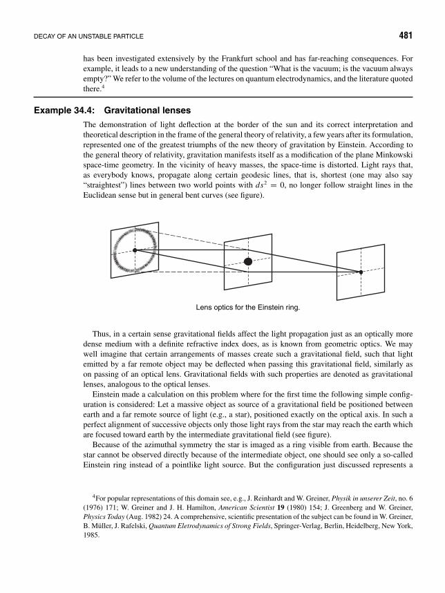
DECAY OF AN UNSTABLE PARTICLE 481
has been investigated extensively by the Frankfurt school and has far-reaching consequences. Forexample, it leads to a new understanding of the question “What is the vacuum; is the vacuum alwaysempty?” We refer to the volume of the lectures on quantum electrodynamics, and the literature quotedthere.4
Example 34.4: Gravitational lenses
The demonstration of light deflection at the border of the sun and its correct interpretation andtheoretical description in the frame of the general theory of relativity, a few years after its formulation,represented one of the greatest triumphs of the new theory of gravitation by Einstein. According tothe general theory of relativity, gravitation manifests itself as a modification of the plane Minkowskispace-time geometry. In the vicinity of heavy masses, the space-time is distorted. Light rays that,as everybody knows, propagate along certain geodesic lines, that is, shortest (one may also say“straightest”) lines between two world points with ds2 = 0, no longer follow straight lines in theEuclidean sense but in general bent curves (see figure).
Lens optics for the Einstein ring.
Thus, in a certain sense gravitational fields affect the light propagation just as an optically moredense medium with a definite refractive index does, as is known from geometric optics. We maywell imagine that certain arrangements of masses create such a gravitational field, such that lightemitted by a far remote object may be deflected when passing this gravitational field, similarly ason passing of an optical lens. Gravitational fields with such properties are denoted as gravitationallenses, analogous to the optical lenses.
Einstein made a calculation on this problem where for the first time the following simple config-uration is considered: Let a massive object as source of a gravitational field be positioned betweenearth and a far remote source of light (e.g., a star), positioned exactly on the optical axis. In such aperfect alignment of successive objects only those light rays from the star may reach the earth whichare focused toward earth by the intermediate gravitational field (see figure).
Because of the azimuthal symmetry the star is imaged as a ring visible from earth. Because thestar cannot be observed directly because of the intermediate object, one should see only a so-calledEinstein ring instead of a pointlike light source. But the configuration just discussed represents a
4For popular representations of this domain see, e.g., J. Reinhardt and W. Greiner, Physik in unserer Zeit, no. 6(1976) 171; W. Greiner and J. H. Hamilton, American Scientist 19 (1980) 154; J. Greenberg and W. Greiner,Physics Today (Aug. 1982) 24. A comprehensive, scientific presentation of the subject can be found in W. Greiner,B. Muller, J. Rafelski, Quantum Eletrodynamics of Strong Fields, Springer-Verlag, Berlin, Heidelberg, New York,1985.

482 APPLICATIONS OF THE SPECIAL THEORY OF RELATIVITY 34
ApparentPosition
StarSun
Earth
Deflection of light at the rim of the sun.
particularly simple idealized case, and it may be highly unlikely to observe exactly such a situation.In any case one may calculate the imaging properties of general lens systems. It turns out that, besidessuch ringlike images, there is also a chance for double or triple images of an object.
Particularly interesting objects of astronomy are quasars, known since 1963. Quasars are starlike(i.e., pointlike as seen from earth) light and radio sources displaying a strong red shift in the spectra.Therefore, they cannot be stars of our Milky Way but rather are very far remote objects, the red shiftof which is a consequence of the expansion of the universe.
In 1979 a pair of very closely spaced quasars was detected. The analysis of their spectra showedthat these agree both in the relative intensity of the spectral lines as well as in their red shift. Furtherobservations have shown that there is a galaxy with low red shift (i.e., closer to us) just between thetwo quasars. Hence it became likely that the double-quasar does not consist of two distinct objectsbut that the astronomers—because of the light deflection in the gravitational field of the galaxy—(see Problem 33.3) see two images of a single object.5 Meanwhile, many more double- and eventriple-images of quasars by gravitational lensing have been detected.
The wave fronts emerging from the light source (quasar) are folded in the vicinity of a large mass(galaxy) such that three wave fronts are passing the observer (see figure). On earth one therefore seesthree images of the quasar. That one sees only two images in the case of double-quasars may be dueto the circumstance that one of the images is very faint or that two images are so closely spaced thatthey are no longer separated optically.
The gravitational lens effect may be observed only in the radiation from quasars since the deflectionangle as seen from earth is proportional to the gravitational potential of the lens at the position of earth.An estimation of the mass distribution in the universe shows that the probability of a gravitationallens effect with a remote galaxy as lens is by about the factor 104 larger than the probability of suchan effect with a star from our Milky Way as deflecting mass.
The first observations of gravitational lensing very done with arrays of radio telescopes. Thistechnique yielded in 1987 the dicovery of an almost perfect Einstein ring.6
Meanwhile, with the advent of the Hubble space telescope and large, modern ground-basedtelescopes with adaptive optics, the observation of gravitational lenses has become very common in
5For an account by one of the discoverers of this first “double-quasar”, see F. H. Chaffee: The Discovery of aGravitational Lens, Scientific American, November 1980, 60–68.
6Jaqueline. N. Hewitt et al.: Unusual Radio Source MG 1131+0456—A Possible Einstein Ring Nature 333,537-540 (1988). An overview from this period is given by Edwin L. Turner: Gravitational Lenses, ScientificAmerican, July 1988, 26-32.

DECAY OF AN UNSTABLE PARTICLE 483
Quasar
Observer
Galaxy
Propagation of a wave front by a galaxy leading to a gravitational lens.
astronomy. It is even used as a tool to extend the range of possible observations and to explore intonew issues such as the quest for dark matter or the history of the universe.7
Thus, by observing gravitational lens systems, one hopes to clarify a number of highly interestingproblems. The light observed has passed cosmic distances. Therefore, gravitational lenses should beaffected already by the geometry of space-time as a whole. As the optical properties of a gravitationallens can be calculated exactly, one may take also the influence of the expansion of the universe intoaccount. In principle it will be possible to determine the so-called Hubble constant, which, roughlyspeaking, connects the extension and the expansion velocity of the universe. A further interestingaspect arises concerning the so-called dark matter as discussed earlier in Section 28. Gravitationallenses must not necessarily be constituted of mass distributions (e.g., quasars, galaxies) that are visiblevia their electromagnetic radiation. From the relative rate of gravitational lens phenomena, one nowmight also conclude on the rate of distributions of dark matter in the universe. An estimation of theirmass would then have a bearing on the decision between cosmologic models, which all involve amean mass density as parameter. We shall stop with these remarks and may wait with the expectationfor further observations that will make the solution of these problem areas more accessible.
7Examples for the various modern “applications” of gravitational lenses are give in the article by JoachimWambsganss: Gravity’s Kaleidoscope, Scientific American, November 2001, 52-59. See also our remarks inconnection with the dark matter problem in Chapter 28.

Index
K -meson, 452π -meson, 451, 455
aberration formula, 405aberration relation, 410acceleration, 42, 58, 73accretion theory, 314addition theorem of velocities, 385, 419angular momentum, 149, 153angular velocity, 81, 230aphelion, 295apogee, 295arc length, 49, 61area theorem, 247association law, 3asteroid, 295astronomy, 295azimuthal acceleration, 79
base, 9base vector, 68base vectors, 10base vectors, unitary, 97basic vectors, 9Big Bang, 135binomial theorem, general, 232binormal vector, 50, 56, 57, 168
cardioide, 78causality principle, 414Cavendish experiment, 253
central force, 150central force field, 114central force problem, relativistic, 474centrifugal potential, 257chain rule, 73, 180characteristic equation, 215, 245circular motion, 43column orthogonality, 373comets, 295commutation law, 3Compton sattering, 465conic sections, 248conservative force, 142contour integral, 87convex surface, 66coordinate areas, 70coordinate frame, 68coordinate frame, Cartesian, 7coordinate frame, curvilinear, 69coordinate frame, reciprocal, 99coordinate lines, 70coordinates, 68coordinates, bipolar, 107coordinates, Cartesian, 69coordinates, natural, 49Copernican world view, 317cosine law, 28Cramer’s rule, 77creeping motion, 218critical damping, 217curl, 87
485
486 INDEX
curvature, 51, 55curvature radius, 52curve, nonplanar, 62curve, plane, 59curves, parallel, 59cyclic permutability, 16, 25cycloid, 234, 236cylindrical coordinates, 71, 73, 78, 80, 103cylindrical coordinates, elliptic, 106cylindrical coordinates, hyperbolic, 106cylindrical coordinates, parabolic, 105
damping, critical, 218Darboux rotation vector, 54de Broglie relation, 447delta operator, 103determinant, 16, 17differential equation, 159, 241differential equation of second order, 197differential quotient, 39differentiation, 40, 41differentiation of a vector, 40Dirac equation, 447Dirac sea, 448direction cosine, 34, 373direction cosines, 30distance vector, 27distance, spacelike, 413distance, timelike, 413divergence, 83, 85, 101Doppler shift, 407, 411dynamic friction, 172
eccentricity, 249ecliptic, 296Einstein’s box, 435ellipse, 249elliptic integral, 232energy law, 144energy, kinetic, 142equation of plane, 28equation of straight line, 28equipotential area, 84ether, 364Euler formulas, 212, 216evolute, 56, 58–60evolute, generalization, 62evolvent, 58–60
fermion, 447fictitious force, 156force, 5, 34force constant, 160force field, 109forced vibration, 220four-force, 428four-vector, 374, 378, 380, 425four-velocity, 427Frenet’sfriction, 172friction, Newtonian, 172friction, Stokes, 172
Galileo transformation, 363, 380Galileo-invariant, 364Gauss law, 112Gauss theorem, 114Graßmann expansion theorem, 19gradient, 83, 100gravitational force, 7gravitational lenses, 481group, 383group velocity, 421
harmonic oscillator, 196heart curve, 78helix, 44, 57high tide, 302Hooke’s law, 162, 196hyperbola, 249
impulse of force, 45, 144, 146inertial system, 140, 362initial condition, of a differential equation, 160integration, 45integration of vectors, 44involute, 59
Jacobi determinant, 100
kinetic energy, 433Kronecker symbol, 8
Laplace expansion theorem, 22law of areas, 151left frames, 7left-handed helix, 44

INDEX 487
lemniscate, 267length contraction, 394, 396length contraction, classical, 395Lenz vector, 277light cone, 414light vectors, 381lightlike distance, 414line integral, 109linear combination, 9, 68local group, 324logarithmic decrement, 216, 225loop integral, 88, 89Lorentz contraction, 417Lorentz scalar, 426Lorentz transformation, 370, 378Lorentzlow tide, 302
magnitude, 2mass, heavy, 164mass, inert, 164matrix, 16matrix product, 31matrix, transposed, 17meridian, 76meteors, 295metric coefficients, 98metric tensor, 98Michelson–Morley experiment, 364Milky Way, 308Minkowski space, 374, 381momentum, 136muons, 391
neap tide, 302nebular theory, 314Newton’s axioms, 134, 135normal acceleration, 81normal plane, 58normal vector, 56, 57, 65, 168nuclear fission, 454nuclear reactions, 469null vector, 3nutation, of earth, 304
operator, 83orientable surface, 66orientation, 68
orthogonality, column, 373orthogonality,oscillator potential, 160osculating plane, 58
pair annihilation, 456pair of forces, 33parabola, 249parallelepipedon, 26parallelogram, 13, 14parity transformation, 18partial derivative, 64path integral, 109pendulum, 202, 229pendulum, ballistic, 147perigee, 295perihelion, 295perihelion motion, 356period, 296phase velocity, 421photon, 448planetoid, 295planets, 295point mechanics, 135point-direction form, 28polygon of forces, 32position vector, 12positron, 448potential, 143potential, effective, 261, 290power, 142power series, 210precession, of earth, 304principal normal vector, 50product rule, 52projection, 27proper time, 427Ptolemaic world view, 315
radial acceleration, 79, 81rapidity, 387rectifying plane, 58reduced mass, 274referencerelativistic energy law, 445relativity principle, 362, 368, 370relativity principle, classical, 140resonance, 222

488 INDEX
resonance catastrophe, 222rest energy, 434rest mass, 428resultant, 3right frames, 7right-handed frame, 69right-handed helix, 13, 44rope pulley, 137rotation, 83, 87, 102rotation matrix, 29rotation matrix, transposed, 31row orthogonality, 373
Sarrus rule, 17satellites, 295scalar, 2scalar field, 83scalar product, 5scaling factors, 71, 96secant, 42shooting stars, 305sink, 87solar system, 296solid angle, 115source, 87space curve, 64space reflection, 18space-time, 412spacelikespherical coordinates, 74, 104spring tide, 302stars, 295static friction, 173Stokes law, 117submatrix, 22suns, 295superposition principle, 136, 198, 244surface integral, 125
tangent plane, 65tangent unit vector, 50tangent vector, 50, 55, 57, 168tangential acceleration, 82tautochrone, 237Taylor expansion, 84, 210Taylor series, 196, 212Thales, theorem of, 29throw, inclined, 166
throw, vertical, 164tidal theory, 313tides, 301time dilatation, 389, 392, 417time of throw, 167timelike distance, 413torque, 33, 34, 149, 153torsion, 52, 55, 56torsion radius, 52, 58total differential, 84, 142transient process, 221transposed matrix, 373trihedral, moving, 49, 57, 169trihedral, reciprocal, 98triple scalar product, 25, 72, 90Tscherenkov radiation, 443tunnel effect, 293twin paradox, 458
ultraviolet shift, 408unit vector, 6unit vectors, Cartesian, 7unit vectors, variable, 71unwinding curve, 59
vector, 2vector density, 45vector field, 83vector flow, 85vector polygon, 9vector product, 13, 16, 18vector product, double, 18vector, axial, 13, 18vector, normal, 56vector, polar, 18velocity, 42, 58, 73volume integral, 130vortex, 87
wave equation, 382work, 109, 141work, mechanical, 5world line, 412world vector, 425
zero meridian, 69zero vector, 3


