33
Classical Linear Regression Model • Normality Assumption • Hypothesis Testing Under Normality • Maximum Likelihood Estimator • Generalized Least Squares
| Date post: | 21-Dec-2015 |
| Category: |
Documents |
| View: | 253 times |
| Download: | 2 times |
Classical Linear Regression Model
• Normality Assumption
• Hypothesis Testing Under Normality
• Maximum Likelihood Estimator
• Generalized Least Squares
Normality Assumption
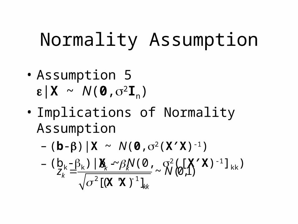
• Assumption 5|X ~ N(0,2In)
• Implications of Normality Assumption– (b-)|X ~ N(0,2(X′X)-1)
– (bk-k)|X ~ N(0, 2([X′X)-1]kk)
2 1~ (0,1)
[( ' ) ]k k
k
kk
bz N
X X
Hypothesis Testing under Normality
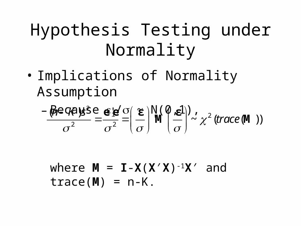
• Implications of Normality Assumption– Because i/ ~ N(0,1),
where M = I-X(X′X)-1X′ and trace(M) = n-K.
22
2 2
( ) '' ~ ( ( ))
n K strace
e e ε ε
M M
Hypothesis Testing under Normality
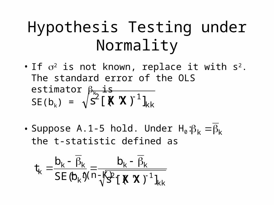
• If 2 is not known, replace it with s2. The standard error of the OLS estimator k isSE(bk) =
• Suppose A.1-5 hold. Under H0:the t-statistic defined as
~ t(n-K).
kk
kk12 ])'[(s XX
kk12
kk
k
kkk
])'[(s
b
)b(SE
bt
XX
Hypothesis Testing under Normality
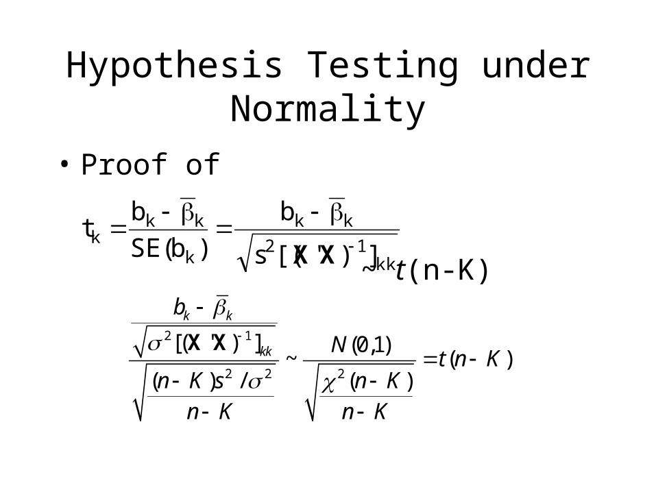
• Proof of
~ t(n-K)kk
12
kk
k
kkk
])'[(s
b
)b(SE
bt
XX
2 1
2 2 2
[( ' ) ] (0,1)~ ( )
( ) / ( )
k k
kk
b
Nt n K
n K s n Kn K n K
X X
Hypothesis Testing under Normality
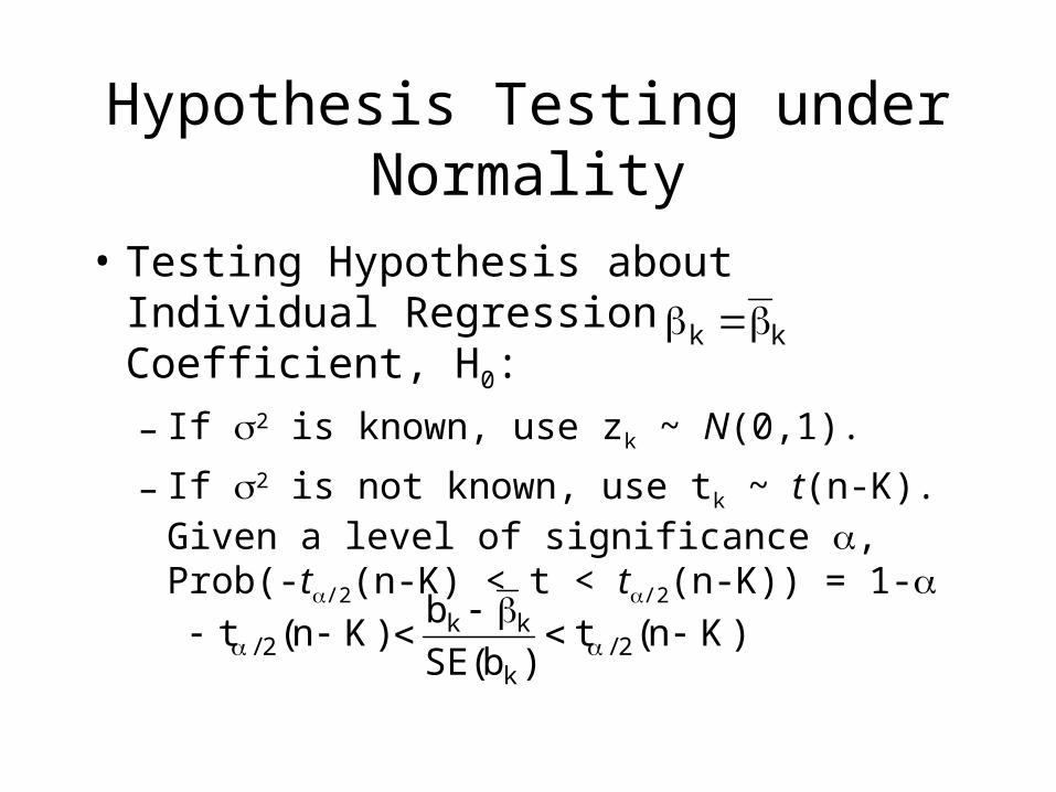
• Testing Hypothesis about Individual Regression Coefficient, H0:
– If 2 is known, use zk ~ N(0,1).
– If 2 is not known, use tk ~ t(n-K).Given a level of significance , Prob(-t/2(n-K) < t < t/2(n-K)) = 1-
kk
)Kn(t)b(SE
b)Kn(t 2/
k
kk2/

Hypothesis Testing under Normality
– Confidence Interval
[bk-SE(bk) t/2(n-K), bk+SE(bk) t/2(n-K)]
– p-Value: p = Prob(t>|tk|)x2Prob(-|tk|<t<|tk|) = 1-psince Prob(t>|tk|) = Prob(t<-|tk|).Accept H0 if p >. Reject otherwise.
)Kn(t)b(SEb)Kn(t)b(SEb 2/kkk2/kk
Hypothesis Testing under Normality
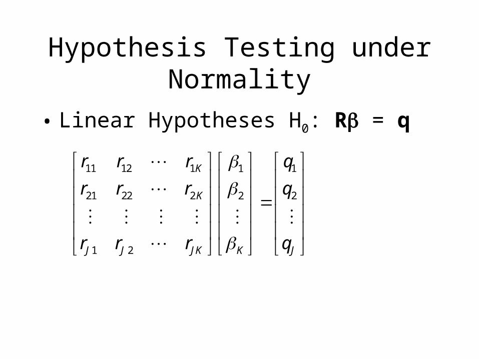
• Linear Hypotheses H0: R = q
11 12 1 11
21 22 2 22
1 2
K
K
J J JK JK
r r r q
r r r q
r r r q
Hypothesis Testing under Normality
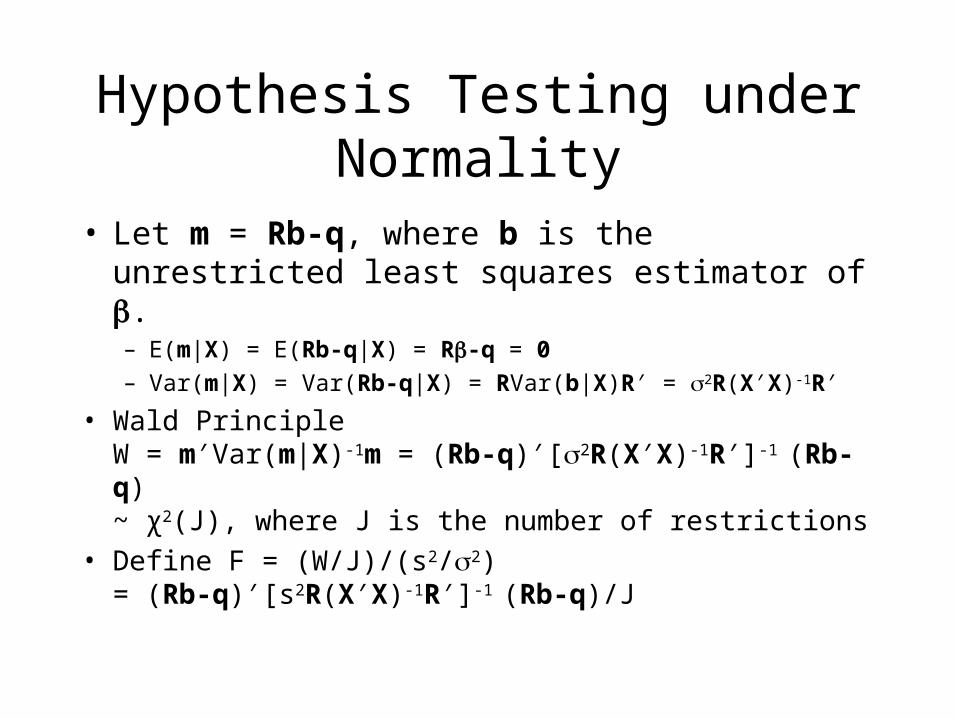
• Let m = Rb-q, where b is the unrestricted least squares estimator of .– E(m|X) = E(Rb-q|X) = R-q = 0
– Var(m|X) = Var(Rb-q|X) = RVar(b|X)R′ = 2R(X′X)-1R′
• Wald PrincipleW = m′Var(m|X)-1m = (Rb-q)′[2R(X′X)-1R′]-1 (Rb-q)~ χ2(J), where J is the number of restrictions
• Define F = (W/J)/(s2/2) = (Rb-q)′[s2R(X′X)-1R′]-1 (Rb-q)/J
Hypothesis Testing under Normality
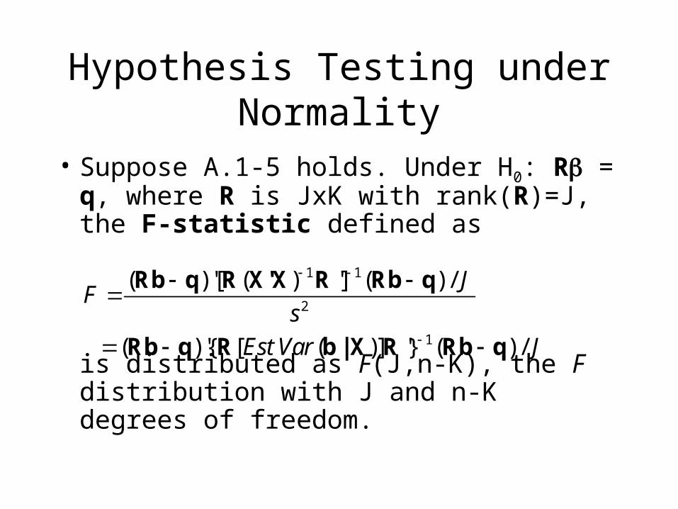
• Suppose A.1-5 holds. Under H0: R = q, where R is JxK with rank(R)=J, the F-statistic defined as
is distributed as F(J,n-K), the F distribution with J and n-K degrees of freedom.
1 1
2
1
( ) '[ ( ) '] ( ) /
( ) '{ [ ( )] '} ( ) /
JF
s
Est Var J
Rb q R X'X R Rb q
Rb q R b | X R Rb q
Discussions
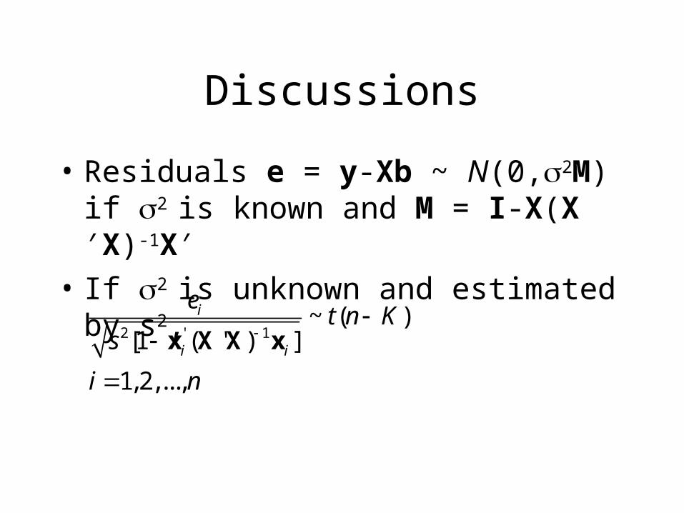
• Residuals e = y-Xb ~ N(0,2M) if 2 is known and M = I-X(X′X)-1X′
• If 2 is unknown and estimated by s2,
2 ' 1~ ( )
[1 ( ' ) ]
1,2,...,
i
i i
et n K
s
i n
x X X x
Discussions
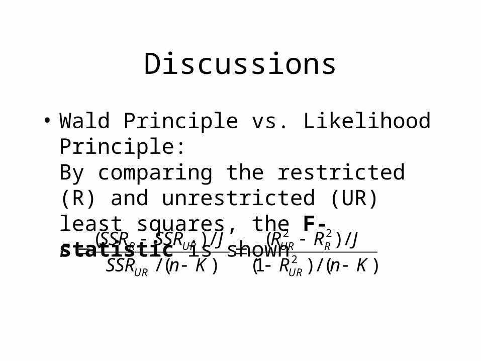
• Wald Principle vs. Likelihood Principle:By comparing the restricted (R) and unrestricted (UR) least squares, the F-statistic is shown
2 2
2
( ) / ( ) /
/ ( ) (1 ) / ( )R UR UR R
UR UR
SSR SSR J R R JF
SSR n K R n K
Discussions
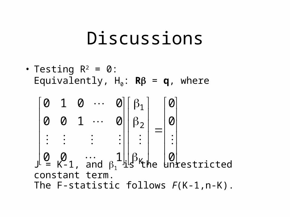
• Testing R2 = 0:Equivalently, H0: R = q, where
J = K-1, and 1 is the unrestricted constant term.The F-statistic follows F(K-1,n-K).
0
0
0
100
0100
0010
K
2
1
Discussions
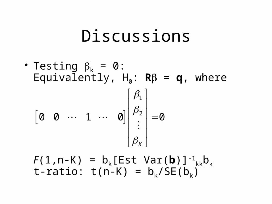
• Testing k = 0:Equivalently, H0: R = q, where
F(1,n-K) = bk[Est Var(b)]-1kkbk
t-ratio: t(n-K) = bk/SE(bk)
1
20 0 1 0 0
K
Discussions
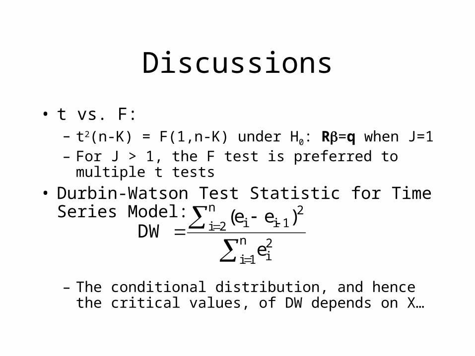
• t vs. F:– t2(n-K) = F(1,n-K) under H0: R=q when J=1 – For J > 1, the F test is preferred to multiple t tests
• Durbin-Watson Test Statistic for Time Series Model:
– The conditional distribution, and hence the critical values, of DW depends on X…
n
1i2i
n
2i2
1ii
e
)ee(DW
Maximum Likelihood
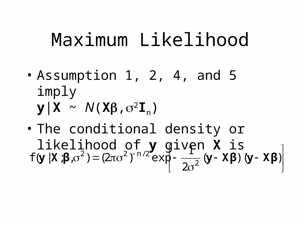
• Assumption 1, 2, 4, and 5 implyy|X ~ N(X,2In)
• The conditional density or likelihood of y given X is
)()'(
2
1exp)2(),;|(f
22/n22 XβyXβyβXy
Maximum Likelihood
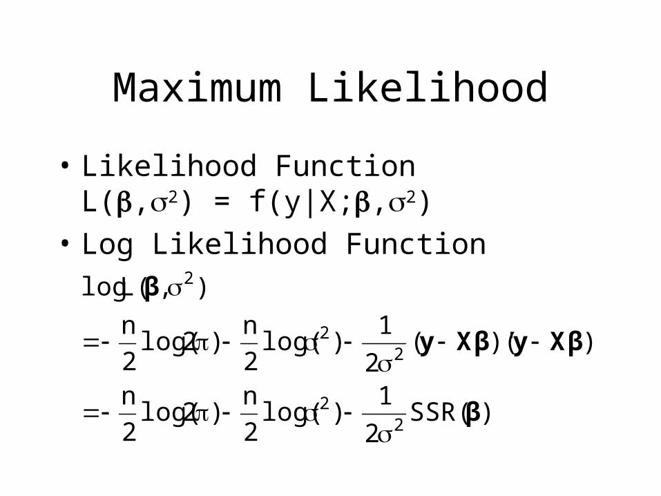
• Likelihood FunctionL(,2) = f(y|X;,2)
• Log Likelihood Function
)(SSR2
1)log(
2
n)2log(
2
n
)()'(2
1)log(
2
n)2log(
2
n
),(Llog
22
22
2
β
XβyXβy
β
Maximum Likelihood
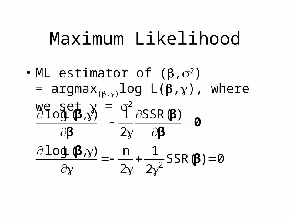
• ML estimator of (,2) = argmax(,)log L(,), where we set = 2
0)(SSR2
1
2
n),(Llog
)(SSR
2
1),(Llog
2
ββ
0β
β
β
β
Maximum Likelihood
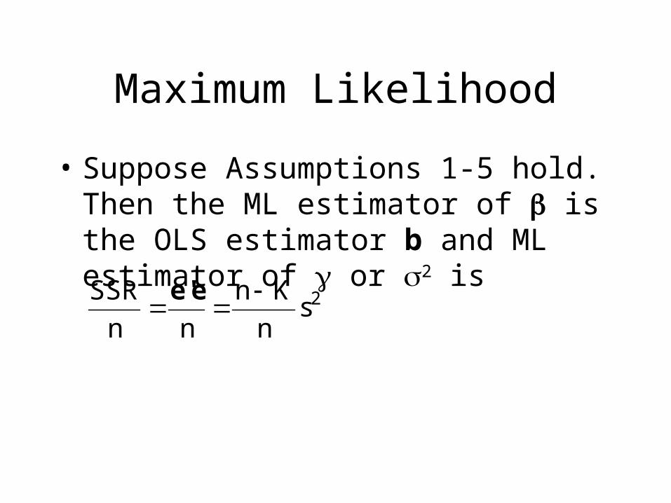
• Suppose Assumptions 1-5 hold. Then the ML estimator of is the OLS estimator b and ML estimator of or 2 is
2sn
Kn
nn
SSR
ee'
Maximum Likelihood
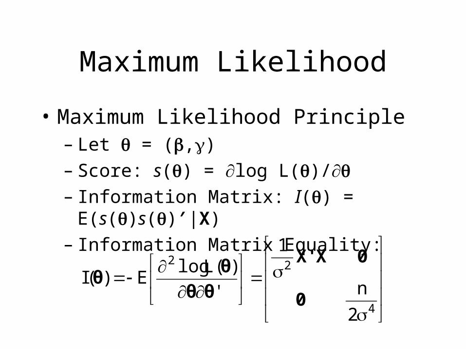
• Maximum Likelihood Principle– Let = (,)– Score: s() = log L()/– Information Matrix: I() = E(s()s()′|X) – Information Matrix Equality:
4
22
2
n
1
'
)(LlogE)(I
0
0XX'
θθ
θθ
Maximum Likelihood
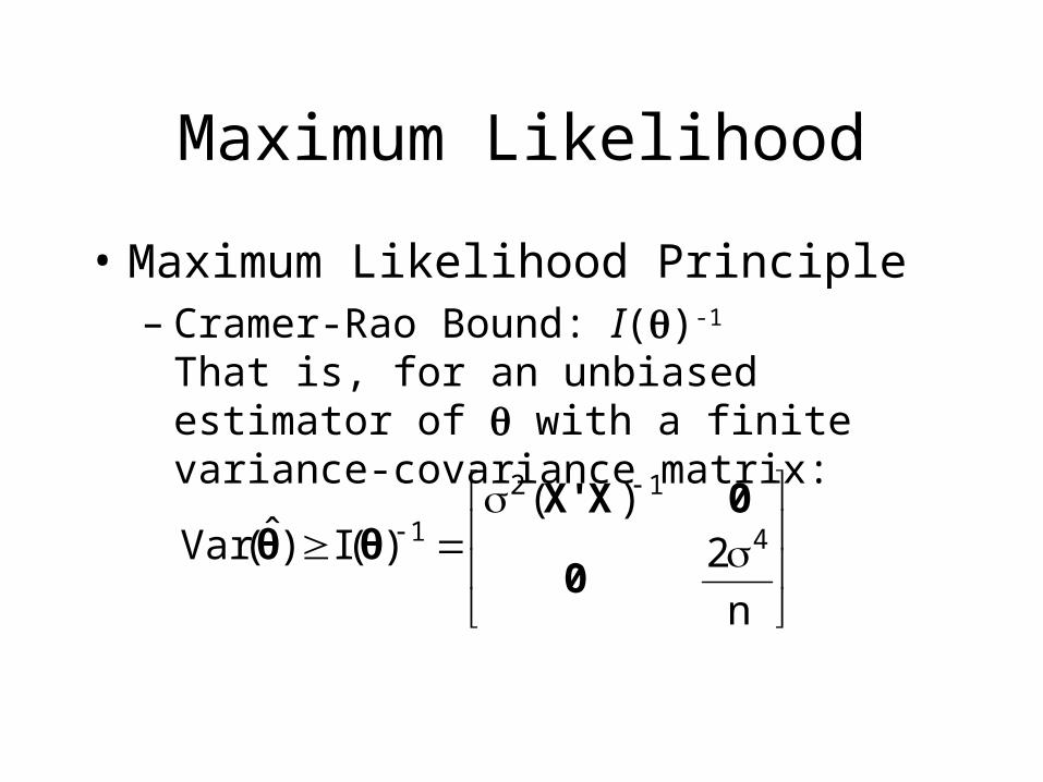
• Maximum Likelihood Principle– Cramer-Rao Bound: I()-1
That is, for an unbiased estimator of with a finite variance-covariance matrix:
n
2)(
)(I)ˆ(Var 4
12
1
0
0XX'θθ
Maximum Likelihood
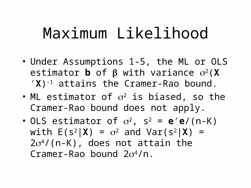
• Under Assumptions 1-5, the ML or OLS estimator b of with variance 2(X′X)-1 attains the Cramer-Rao bound.
• ML estimator of 2 is biased, so the Cramer-Rao bound does not apply.
• OLS estimator of 2, s2 = e′e/(n-K) with E(s2|X) = 2 and Var(s2|X) = 24/(n-K), does not attain the Cramer-Rao bound 24/n.
Discussions
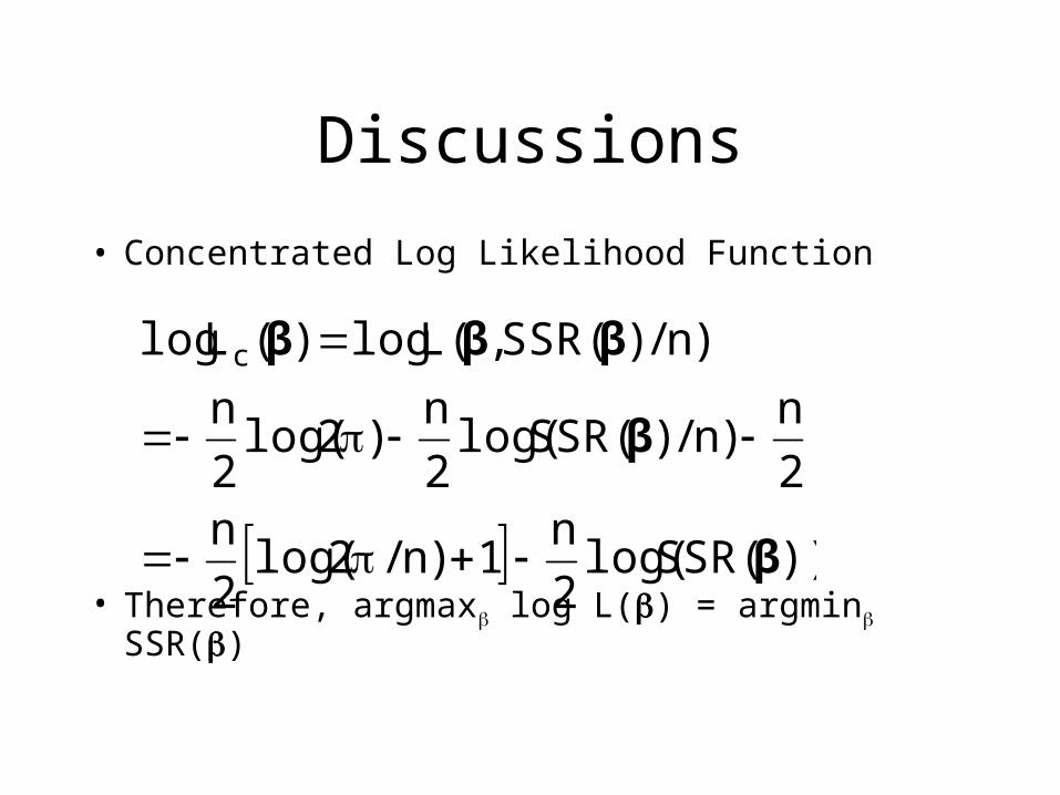
• Concentrated Log Likelihood Function
• Therefore, argmax log L() = argmin SSR()
))(SSRlog(2
n1)n/2log(
2
n2
n)n/)(SSRlog(
2
n)2log(
2
n
)n/)(SSR,(Llog)(Llog c
β
β
βββ
Discussions
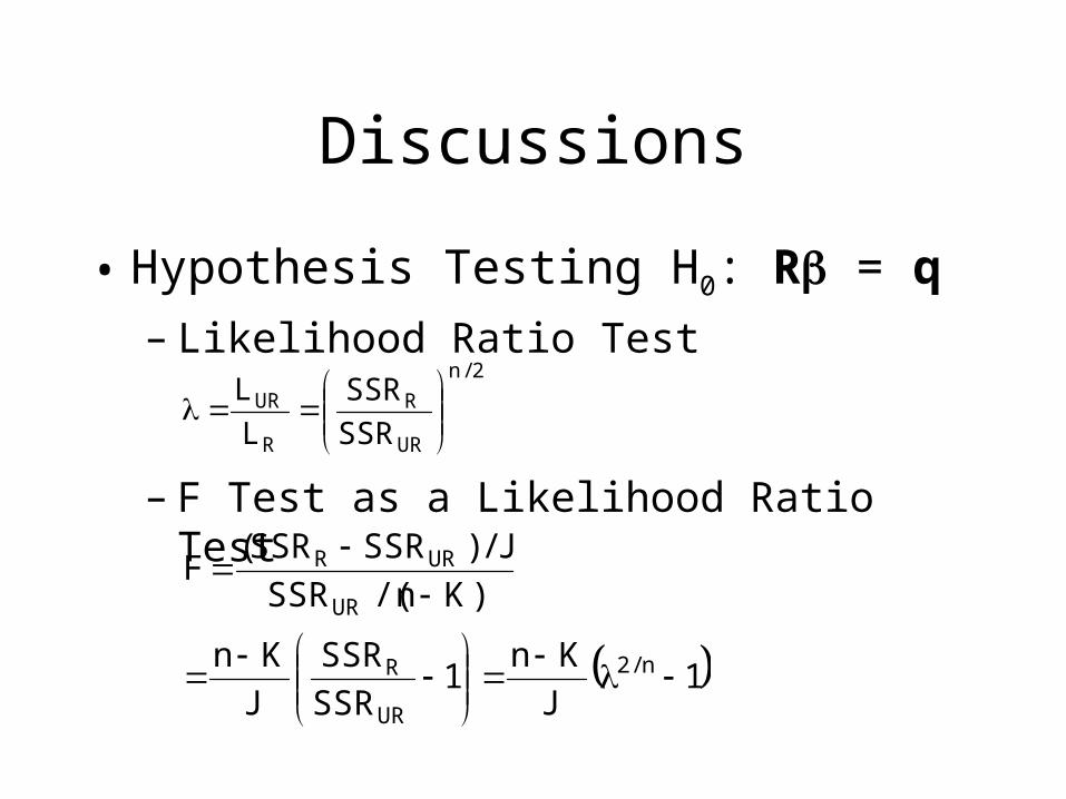
• Hypothesis Testing H0: R = q
– Likelihood Ratio Test
– F Test as a Likelihood Ratio Test
1J
Kn1
SSR
SSR
J
Kn
)Kn/(SSR
J/)SSRSSR(F
n/2
UR
R
UR
URR
2/n
UR
R
R
UR
SSR
SSR
L
L
Discussions
• Quasi-Maximum Likelihood– Without normality (Assumption 5), there is no
guarantee that ML estimator of is OLS or that the OLS estimator b achieves the Cramer-Rao bound.
– However, b is a quasi- (or pseudo-) maximum likelihood estimator, an estimator that maximizes a misspecified (normal) likelihood function.
Generalized Least Squares
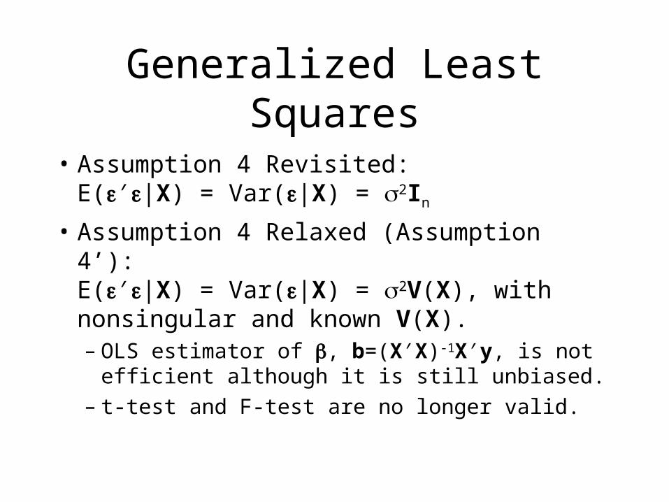
• Assumption 4 Revisited:E(′|X) = Var(|X) = 2In
• Assumption 4 Relaxed (Assumption 4’):E(′|X) = Var(|X) = 2V(X), with nonsingular and known V(X).– OLS estimator of , b=(X′X)-1X′y, is not
efficient although it is still unbiased.– t-test and F-test are no longer valid.
Generalized Least Squares
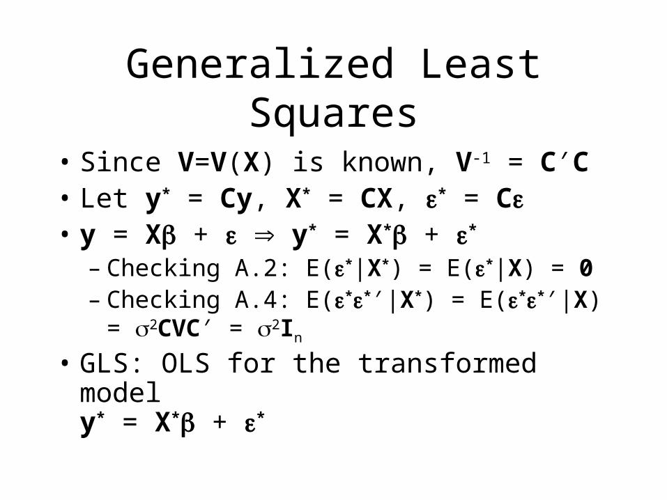
• Since V=V(X) is known, V-1 = C′C • Let y* = Cy, X* = CX, * = C• y = X + y* = X* + *
– Checking A.2: E(*|X*) = E(*|X) = 0 – Checking A.4: E(**′|X*) = E(**′|X) =
2CVC′ = 2In
• GLS: OLS for the transformed modely* = X* + *
Generalized Least Squares
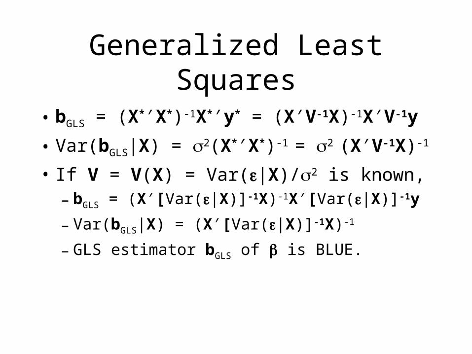
• bGLS = (X*′X*)-1X*′y* = (X′V-1X)-1X′V-1y
• Var(bGLS|X) = 2(X*′X*)-1 = 2 (X′V-1X)-1
• If V = V(X) = Var(|X)/2 is known,– bGLS = (X′[Var(|X)]-1X)-1X′[Var(|X)]-1y
– Var(bGLS|X) = (X′[Var(|X)]-1X)-1
– GLS estimator bGLS of is BLUE.
Generalized Least Squares
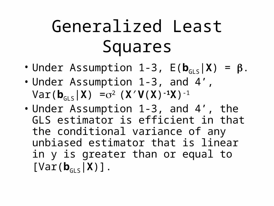
• Under Assumption 1-3, E(bGLS|X) = .• Under Assumption 1-3, and 4’,
Var(bGLS|X) =2 (X′V(X)-1X)-1
• Under Assumption 1-3, and 4’, the GLS estimator is efficient in that the conditional variance of any unbiased estimator that is linear in y is greater than or equal to [Var(bGLS|X)].
Discussions
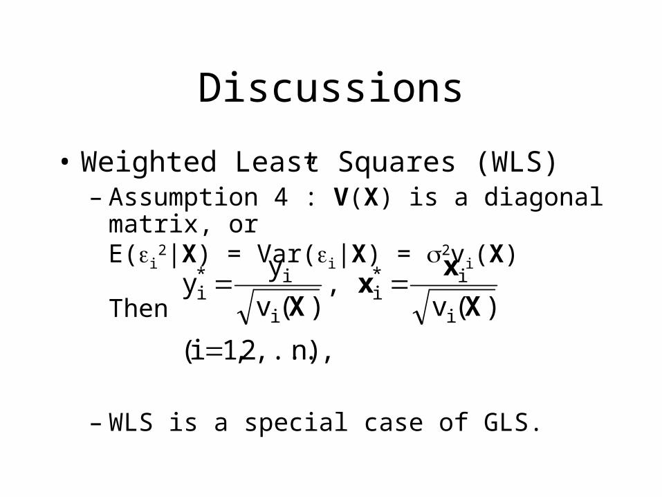
• Weighted Least Squares (WLS)– Assumption 4”: V(X) is a diagonal matrix, or
E(i2|X) = Var(i|X) = 2vi(X)
Then
– WLS is a special case of GLS.
)n,...,2,1i(
)(v,
)(v
yy
i
i*i
i
i*i
X
xx
X
Discussions
• If V = V(X) is not known, we can estimate its functional form from the sample. This approach is called the Feasible GLS. V becomes a random variable, then very little is known about the distribution and finite sample properties of the GLS estimator.
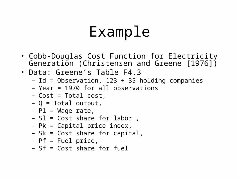
Example
• Cobb-Douglas Cost Function for Electricity Generation (Christensen and Greene [1976])
• Data: Greene’s Table F4.3 – Id = Observation, 123 + 35 holding companies– Year = 1970 for all observations – Cost = Total cost, – Q = Total output, – Pl = Wage rate, – Sl = Cost share for labor , – Pk = Capital price index, – Sk = Cost share for capital, – Pf = Fuel price, – Sf = Cost share for fuel
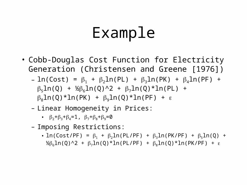
Example
• Cobb-Douglas Cost Function for Electricity Generation (Christensen and Greene [1976])– ln(Cost) = 1 + 2ln(PL) + 3ln(PK) + 4ln(PF) + 5ln(Q)
+ ½6ln(Q)^2 + 7ln(Q)*ln(PL) + 8ln(Q)*ln(PK) + 9ln(Q)*ln(PF) +
– Linear Homogeneity in Prices:• 2+3+4=1, 7+8+9=0
– Imposing Restrictions:• ln(Cost/PF) = 1 + 2ln(PL/PF) + 3ln(PK/PF) + 5ln(Q) +
½6ln(Q)^2 + 7ln(Q)*ln(PL/PF) + 8ln(Q)*ln(PK/PF) +


