A. Vasylchenkova, M. Mraz, N. Zimic, and M. Moškon, Classical mechanics approach applied to analysis of genetic oscillators, preprints in IEEE/ACM Transactions of Computational Biology and Bioinformatics (doi: 10.1109/TCBB.2016.2550456)
Abstract—Biological oscillators present a fundamental part of several regulatory mechanisms that control the response of variousbiological systems. Several analytical approaches for their analysis have been reported recently. They are, however, limited to onlyspecific oscillator topologies and/or to giving only qualitative answers, i.e., is the dynamics of an oscillator given the parameter spaceoscillatory or not. Here we present a general analytical approach that can be applied to the analysis of biological oscillators. It relies onthe projection of biological systems to classical mechanics systems. The approach is able to provide us with relatively accurate resultsin the meaning of type of behaviour system reflects (i.e. oscillatory or not) and periods of potential oscillations without the necessity toconduct expensive numerical simulations. We demonstrate and verify the proposed approach on three different implementations ofamplified negative feedback oscillator.
Index Terms—Oscillatory Dynamics, Genetic Oscillators, Ordinary Differential Equations, Dynamical Systems.
F
1 INTRODUCTION
ANALYSIS of biological oscillators is important in contextof natural as well as synthetic biological systems.
In-silico investigation of behaviour of different synthetictopologies that reflect oscillatory behaviour in certain condi-tions is able to guide the implementation of biological sys-tems with desired functionality [1], [2]. Analysis of naturaloscillators is, on the other hand, important for understand-ing of underlying mechanisms that regulate several cellularresponses, such as circadian clocks or cell cycle oscillators[3], [4].
Genetic oscillator analyses have been a subject of in-depth investigation recently following the first successfulin vivo implementation of the repressilator circuit [5]. Therepressilator and its generalized models were thoroughlyanalysed by different authors [6], [7], [8]. Comparative anal-ysis of design principles in biochemical oscillators, oscillatortopologies or only variations in their implementations havealso been performed by several researchers [1], [2], [9],[10]. The most straightforward approach to the quantitativeanalysis of oscillatory behaviour used in existent studiesis to perform numerical simulations on different oscillatormodels, and analyse the time evolution of observed chem-ical species in dependence on chemical kinetic rates andinitial conditions (for example see [10]). However, main dis-advantages of this approach are in inherent expensivenessof numerical simulations and additionally in dependence oninitial conditions, i.e. on initial species concentrations.
Another strategy is to use various analytical approacheswhich do not rely on repetitive iterations of expensive
• A. Vasylchenkova is with the School of Physics and Technologies, V. N.Karazin Kharkiv National University, Kharkiv, Ukraine.
• M. Mraz, N. Zimic and M. Moskon are with the Faculty of Computer andInformation Science, University of Ljubljana, Ljubljana, Slovenia.
Manuscript received ; revised .
numerical simulations. These are in most cases limited toonly specific systems and/or bifurcation types. For example,search for the existence of stable limit cycles can be per-formed analytically. It is very difficult to determine whetherthe equations that describe the system will reflect oscillatorybehaviour or not in general [11]. In some cases, however,it is possible to determine parameter ranges for which thesystem exhibits oscillatory behaviour. Repressilator topol-ogy, for example, only exhibits Hopf bifurcation and canbe analysed thoroughly with the linearisation of its modeland investigation of the eigenvalues of the linearised system[5], [6]. It is also possible to evaluate oscillation periodsnear the bifurcation points when oscillations emerge from asupercritical Hopf bifurcation. If other types of bifurcationsoccur, or if we are interested in the dynamics far frombifurcation points, other methods need to be applied.
Existing analytical approaches mostly allow us to onlyperform the qualitative analysis, e.g., see [12]. Some effortshave been made recently to also obtain the quantitative in-formation of oscillatory response. Analytical approximationof oscillation frequency and period derived specifically fortwo different oscillator topologies, i.e. circadian oscillatormodel according to [13] and repressilator model accordingto [5], has been reported [14]. Authors show that the oscilla-tion frequency and period can be approximated with a sat-isfactory accuracy with analytical investigation of ordinarydifferential equations describing the system’s dynamics. Ap-proach presented is, however, limited to only two differenttopologies. In [15] authors present an analytical method thatcan be applied to a genetic oscillator with negative feedbackring topology, i.e. a more generalized model which can alsodescribe the Goodwin oscillator and repressilator [5], [16].This again presents a limitation because the method cannotbe straightforwardly applied to more general topologieswhich also include positive feedbacks. Positive feedbackloops, however, increase the chances of obtaining oscilla-
IEEE/ACM TRANSACTIONS ON COMPUTATIONAL BIOLOGY AND BIOINFORMATICS 2
tions [17], [18], [19], allow the tunability of the oscillationperiods [20], and also introduce a certain degree of non-linearity in the system [21]. Moreover, approaches describedin [14] and [15] rely on the approximation of a promoteractivity with a Boolean variable having two possible values,i.e. zero (not active) and one (active). Promoter dynamicsis thus approximated with a unit step function, whichyields active promoter when activator threshold concen-tration value is exceeded by activators, and/or repressorthreshold concentration value is not exceeded by repressorsat the same time. This presumption is valid only for a verylimited scope of biological systems, i.e. for promoters thatexhibit highly nonlinear response, and is also unable todiffer among certain promoter implementations, e.g., com-petitive versus non-competitive transcription factor binding(see Supplementary material).
Here we present a more general analytical approach,which can be applied to an arbitrary oscillator topology. Itrelies on the projection of the model describing the dynam-ics of a biological system to a classical mechanics system.The projected system can be analysed further on with classi-cal mechanics theory. Described approach is able to provideus with the type of behaviour system reflects (oscillatoryor stationary) and periods of potential oscillation withoutthe necessity to conduct expensive numerical simulations.This allows us to perform the analysis more efficientlyand with less computational effort than with conventionalmodelling and analysis methodologies. The advantages ofproposed methodology become evident especially when weare interested in the dynamics of the system in dependenceon a vast range of parameter values, e.g., when conductinglocal or global sensitivity analysis [22], parameter sweepanalysis, or when exact parameter values are unknown. Inthe latter case, e.g., we need to investigate the dynamics ofthe system using a large scope of different parameter val-ues surrounding presumed nominal parameter estimates.The methodology can be as such efficiently applied to theprocess of design of novel genetic oscillators and also tothe understanding of existing ones, e.g., in the context oftheir sensitivity to environmental changes. Even though wefocus our attention to genetic oscillators only, the proposedmethodology can also be used to analyse other types ofbiological or chemical oscillators or even dynamical systemsin general.
The rest of the paper is organized in the following way.First we introduce and describe the proposed applicationof classical mechanics to biological systems in details. Wedemonstrate the methodology on three different amplifiednegative feedback oscillator models derived from [10]. Weverify the proposed approach with the comparison per-formed on the results obtained with numerical simulations.We conclude the paper with the discussion about the ad-vantages and drawbacks, and give some concrete biologicalapplications and possible future improvements of proposedapproach.
2 METHODS
2.1 Biological systems as dynamical systemsOne of the most common approaches for modelling thedynamics of biological systems, especially gene regulatory
networks, is deterministic modelling. In this case modelsare established on the basis of a system of coupled ordinarydifferential equations (ODEs) [23], [24], which approximatean average response of the network deterministically [25].These equations describe the dynamics of each observedchemical species in the following way:
dxidt
= fi(x(t),p), (1)
where fi is a (usually non-linear) function governing thedynamics of chemical species xi (i ∈ {1, 2, ..., n}) in de-pendence on the state of the system in time step t, i.e.x(t) = (x1(t), x2(t), ..., xn(t)) and in dependence on modelparameters p = (p1, p2, ...). These equations can be estab-lished with the basic mass action kinetics, and can be furthersimplified using, e.g., Michaelis-Menten equations to ap-proximate enzymatic reactions or Hill equations to describegene expression [26]. These can be additionally generalizedwith fractional occupancy [27] or thermodynamic modellingapproach [28]. Due to the nonlinearity of ODEs, their solu-tions are usually obtained with numerical integration. Themain problems of this approach are in dependence on initialconditions and in its computational expensiveness. Compu-tational expensiveness presents a major obstacle especiallywhen parameter values are only partially known, or whenwe are interested in the stability of system’s reponse independence on parameter perturbations. In these two caseslarge amount of simulations needs to be performed in orderto obtain response of the system to a vast range of differentparameter values. Analytical approaches that approximatethe phenotype behind the ODE description of the systemwithout the necessity to conduct expensive numerical sim-ulations have already been proposed for certain biologicalsystem (e.g., see [14], [15] for selected genetic oscillators).State-of-the-art approaches, however, lack generality whilethey can be applied straightforwardly to only selectednetwork topologies, and also make certain presumptionsthat additionally limit the scope of their usability (e.g.,using unit step function to approximate promoter activity- see Supplementary material). We introduce a more generalapproach that can be applied to an arbitrary biologicaloscillator topology to analytically determine its qualitativeand quantitative response.
2.2 Oscillatory behaviour in classical mechanicsClassical mechanics defines oscillatory behaviour as peri-odic changes in body position within the observed space.It occurs in the neighbourhood of some stable position,i.e. equilibrium point (EP), in which either no forces act onthe body, or all the forces are compensated. Oscillatorybehaviour occurs if small perturbation from EP causes theoccurrence of the force in the direction of EP, i.e. returningforce [29]. Let’s consider a 1-dimensional mechanical systemalong unique coordinate axis x. In this case all vector quan-tities (such as force) can be used in terms of their projection.If direction of vector coincides with direction of axes, thisvector has a positive projection, otherwise a negative one.
Equations describing the motion are usually given inspecific forms. Solutions of these equations can be inter-preted as the positions of body in motion in dependenceon time. This motion is caused by the forces that result in
IEEE/ACM TRANSACTIONS ON COMPUTATIONAL BIOLOGY AND BIOINFORMATICS 3
the body acceleration, and can be expressed as the secondtime derivative of the body position:
a = x. (2)
Equations describing the motion in classical mechanics aretherefore usually given in the form of the second order dif-ferential equations. Since force F is a function of coordinatex in a 1-dimensional system, EPs (i.e. x0) can be determinedwith the solutions of the equation F (x0) = 0. We canconduct the analysis of the system in the neighbourhoodof the EP with the Taylor series expansion:
F (x) ≈ F (x0) + (x− x0)dF
dx
∣∣∣∣x=x0
+ ... (3)
Zero-order term equals zero as long as x0 is an EP. Higher-order terms can be neglected in the close proximity of the EP.The dynamics in the neighbourhood of the EP is thereforedefined by the first order terms only. Their positive valuesindicate the force directed from the EP. On the contrary,their negative values indicate the existence of the returningforce that presents a necessary condition for the oscillatorybehaviour. Let’s define k as an absolute value of first-orderderivative of F in EP:
k =
∣∣∣∣∣ dFdx∣∣∣∣x=x0
∣∣∣∣∣ , (4)
which equals
k = − dF
dx
∣∣∣∣x=x0
(5)
in the case of the returning force around the EP. The substi-tution of Eq. (5) and equation F = ma, wherem presents thebody mass, to Eqs. (2) and (3) yields the following equation
mx = −k(x− x0), (6)
which can be rewritten as
x = −ω2x. (7)
Here ω2 = km . It is important to note that ω can be inter-
preted as the circular frequency of oscillations. The equationcan be used to express the period of oscillations
T =2π
ω= 2π
√m
k(8)
as a well-known formula for period of spring pendulum,where k can be interpreted as an elastic coefficient of thespring.
Another approach to determine the motion is to usepotential energy function, i.e. a function of coordinates(U = U(x, y) in 2D-case) linked with the forces acting onthe system by the following relations:
Fx = mx = −∂U∂x
,
Fy = my = −∂U∂y
. (9)
Potential energy can be visualized as a surface with somerelief, on which the system can move. Minimums of therelief present the points of stable equilibrium
U(x, y)− min in x0, y0 ≡U ′x = 0 and U ′y = 0 ≡
Fx = Fy = 0. (10)
The potential energy has the following form
U(x, y) =a(x− x0)2
2+b(y − y0)2
2. (11)
for a simple oscillator. Partial derivation of this formulaleads to expression of forces in the form of Equation (6).In this expression a and b can be interpreted as the squaresof circular frequencies ω2
x and ω2y (presuming that m equals
1), from which period can be calculated by Equation (8).Naturally, a and b are positive parameters.
System with such form of potential energy function iscalled a harmonic oscillator. It presents the simplest systemwhich may exhibit oscillatory behaviour, and may be usedto approximate different oscillators. We also use such ide-alized model as an approximation of our original system.The approximation, however, cannot be performed whenno EPs exist. In that case we can immediately deduce thatthe behaviour of the system is not oscillatory (cases withnegative EPs can also be eliminated in the case of biologicalsystems while the concentrations should always be non-negative). Further on, we observe the potential energy of anapproximated system, which presents a necessary conditionfor oscillations to occur. In case the energy is not conservedor when potential energy function cannot be expressed, thesystem will exhibit damped or no oscillation at all (seeSect. 2.3 for further details).
2.3 Classical mechanics in dynamical systems
Dynamical systems can be in general described with thesystem of first order differential equations (ODEs), whichinclude variables that may have different interpretation. Inphysics, these equations describe mechanical motion, wherevariables are interpreted as coordinates of body position.In biological systems, these variables usually describe thedynamics of observed chemical species (see Sect. 2.1). Ourmethodology relies on the approximation of system’s po-tential energy function, which can be performed for anarbitrary oscillatory dynamical system with the calculationof first integral. It therefore does not depend on the back-ground behind the ODE system. Here, however, we focus tothe analysis of biological oscillators.
Let’s presume we are observing the biological systemwhich is comprised of only two chemical species. The dy-namics of this system can be described with the followingset of equations
x = f(x, y,p) = f,
y = g(x, y,p) = g. (12)
The time derivation of these equations brings them to theform of the Equation (7)
x = f ′xx+ f ′y y,
y = g′xx+ g′y y. (13)
According to Leibniz rule, we obtain
x = f ′xf + f ′yg ≡ f(x, y),
y = g′xf + g′yg ≡ g(x, y). (14)
IEEE/ACM TRANSACTIONS ON COMPUTATIONAL BIOLOGY AND BIOINFORMATICS 4
These equations can be expanded in the Taylor series. Onlyfirst order terms need to be regarded here (zero order termsequal 0 in the EPs and higher order terms can be neglected):
x =∂f
∂x|x0,y0(x− x0) +
∂f
∂y|x0,y0(y − y0)
≡ a(x− x0) + b(y − y0),
y =∂g
∂x|x0,y0(x− x0) +
∂g
∂y|x0,y0(y − y0)
≡ c(x− x0) + d(y − y0). (15)
Potential energy for such equations system exists if b = cbecause
∂2U
∂x∂y=
∂2U
∂y∂x. (16)
If this condition is not satisfied, the potential energy func-tion does not exist, and the behaviour of the simplifiedsystem cannot be oscillatory. Otherwise the potential energyhas the following form
U(x, y) = −a(x− x0)2
2− b(x− x0)(y − y0)− d(y − y0)2
2.
(17)As bilinear form, this function can be diagonalized byrotation of coordinate system. This operation is performedby the calculation of eigenvalues of bilinear form matrix:
U(u, v) =λ1(u− u0)2
2+λ2(v − v0)2
2, (18)
where u and v present the new coordinates after rotation,and λ1,2 present the eigenvalues of potential energy matrix,which can be interpreted as the squares of circular frequen-cies of oscillations modes along new axes.
It is possible for the calculated circular frequencies tohave non-zero imaginary parts, which consequences in theabsorption of energy and damped oscillations. However,oscillatory behaviour can be achieved also with non-zeroimaginary parts, which should be substantially smaller thanreal parts. Maximal threshold determining the ratio betweenimaginary and real parts of circular frequencies, for whichoscillatory behaviour is still observed needs to be evaluated.Threshold value that we use in the analysis should minimizethe errors of our approach in comparison to a crediblesource of data, e.g., numerical simulations, on a testing setof parameter values. The process of its estimation for thepurpose of our case study is described in the Supplementarymaterial. The same value can be used on all three modelsor even in a general case. One can alternatively determinespecific threshold values that are optimal for a given modelto obtain more accurate results. Real parts of obtainedcircular frequencies should be positive numbers at the sametime, due to their biological interpretation.
Obtained values of circular frequencies can thus be usedto determine the type of behaviour the system reflects(oscillatory or not), and to determine the periods of potentialoscillations. Oscillation periods can be estimated in the fol-lowing way. Two oscillation modes exist in a 2-dimensionalsystem. Their periods can be expressed as
T1,2 =2π√λ1,2
. (19)
It is possible to obtain different values of periods for eachoscillation mode (i.e., in the case when real parts of obtainedeigenvalues are different). These can be used to calculatea single true value of oscillation periods which is exper-imentally observed, and which presents a minimal timeinterval needed for the system to periodically return toa state that was already reached before. Composition ofoscillations along two orthogonal axes can be visualized,and this visualization is known as Lissajous curves [30]. Let’spresume that oscillations happen with equal frequencies,i.e. both oscillation modes (both dimensions) have the sameoscillation periods, and that the point is in equilibrium statealong one axis (x) and maximally deflected along anotherone (y) at the same time. In quarter of period, coordinatex reaches the maximal amplitude value, and coordinate yreturns to zero. Coordinate y continues decreasing up tomaximal negative deflection. At the same time, coordinate xchanges back to zero. Observed point therefore draws a cir-cle on the coordinate plane. In general the Lissajous curvesare closed curves if frequency ratios are rational numbers.Mathematically this means that some finite time intervalexists in which the state vector periodically returns back toa state that was already reached before. This time intervalpresents the oscillation period of the system. Periods ofoscillation, either observed on a point of mass or on a set ofbiological chemical species, can be therefore calculated as aLeast Common Multiplier (LCM) of periods along separateaxis defined in the following way:
T = LCM(T1, T2)|T, T1, T2 ∈ R, ifT
T1,T
T2∈ N. (20)
Here, oscillation periods of the system and oscillation pe-riods of each of its dimensions are in general non-integernumbers. However, the definition requires that the ratiosamong them are integers.LCM of two rational numbers canalso be obtained in the following, more convenient, way:
LCM(T1, T2) =LCM(m1,m2)
GCF (n1, n2), (21)
where T1 = m1/n1 and T2 = m2/n2 and GCF presentsthe greatest common factor of its arguments (see Supple-mentary material for further details about the calculationof the LCM of two non-integer numbers). This brings usto the last step of proposed methodology. In order to findtrue, observed periods of oscillation, LCM of periods alongseparate axes (i.e. periods of different modes) found inprevious steps should be calculated.
Even though we described the proposed methodologyon a two-dimensional system only, it can be applied toa system with more dimensions in the same way. In thiscase the number of oscillation modes equals the number ofequations describing the system’s dynamics. The oscillationperiods are thus expressed with the LCM of periods of allmodes.
3 RESULTS
3.1 Case studyThe case study will be performed on an amplified negativefeedback oscillator, which presents a very general topologyincluding both positive and negative feedbacks. While this
IEEE/ACM TRANSACTIONS ON COMPUTATIONAL BIOLOGY AND BIOINFORMATICS 5
topology has already been studied extensively, some of itsvariations have also been constructed experimentally (forexample see [17] and [31]). Our analysis will be performedon selected implementations described in [10], namely twovariations of Design I (see Fig. 1(a) and Fig. 1(b)) and onevariation of Design III (see Fig. 1(c)). We only give a briefdescription of the models in the main text. More accuratederivation of these models accompanied with the nominalparameter values is included in Supplementary material ofthe manuscript (see also references [2] and [10]).
Design I implementation presumes that regulation ofthe activator protein is achieved through the competitionbetween the activator and repressor at the activator’s pro-moter. The implementation can be described with the model
dx
dτ= ∆
(β
1 + αxn
1 + xn + σym− x
), (22)
dy
dτ= ∆γ
1 + αxn
1 + xn− y,
where x and y are non-dimensional variables associated tothe activator and repressor, α presents the transcriptionalsynergy of activated promoter, β and γ present the non-dimensional strength of the transcription and translationfor the activator and repressor, σ presents the binding ratioof repressor compared to activator, n and m present theHill coefficients of activator and repressor, ∆ presents theratio between the activator’s and repressor’s degradationrates, and τ presents a non-dimensional time variable (seeSupplementary material).
A variation of Design I (Design I.1) presumes additionalpositive feedback with the autocatalysis on the repressor.This implementation is also known as Smolen oscillator [1],[32]. It can be described with the model
dx
dτ= ∆
(β
1 + αxn
1 + xn + σym− x
), (23)
dy
dτ= ∆γ
1 + αxn
1 + xn + σym− y.
Here, the parameters have the same interpretation as inDesign I.
Design III presumes specific inhibition, where activatorand repressor bind to their designated binding sites, i.e. bothbinding sites at the activator’s promoter can be occupied atthe same time. It can be described with the model
dx
dτ= ∆
(β
1 + αxn
(1 + xn) (1 + σym)− x
), (24)
dy
dτ= ∆γ
1 + αxn
1 + xn− y,
where the parameters have the same interpretation as inDesign I.
3.2 Analysis descriptionThe analysis using the proposed methodology is performedin two steps. In the first step we determine the coordinatesof EPs from the numerical solutions of
dx
dτ= 0,
dy
dτ= 0. (25)
In the second step we construct a potential energy matrix[−a −b−c −d
],
which is obtained with the derivations of initial ODE sys-tem dx
dτ and dydτ (see Equation (15)). First we examine the
symmetry of the potential energy matrix (i.e. we checkthe condition b = c). If the condition is not satisfied,the behaviour of the system is identified to be stationary.Otherwise we further calculate the eigenvalues of potentialenergy matrix (λ1 and λ2), which present the squares ofcircular frequencies of two oscillation modes. Oscillatory be-haviour is obtained only if the complex parts of these valuesare substantially small (see Sect. Evaluating the thresholdvalues in Supplementary material). In this case periods ofboth oscillation modes can be expressed with the equationT1,2 = 2π/Re(λ1,2). Finally, oscillation period is calculatedas the LCM of periods of both modes.
Numerical analysis was performed additionally to verifythe results of proposed methodology. It was conducted withthe numerical integration of ODEs described in Sect. 3.1. Theoscillatory behaviour was analysed on the time evolutionof observed proteins’ concentrations. In order to disregardthe initial transient effects the signal was analysed fromthe second half of the simulation time onwards. Simulationtime was sufficiently long for the transient effects to dieout in each analysed scenario. The analysis was performedwith the localization of the signal peaks and comparison oftime delays between the peaks. If time delays were regularenough, the dynamics of the signal was treated as periodic.
Most of the calculations were performed with MAT-LAB. Numerical integration and the analysis of the re-sults obtained with the integration were performed withGNU C Compiler (gcc) and GNU Scientific Library (GSL)[33]. Numerical analysis was based on the improved codeprovided in the Supplementary material of [10]. All thecode used in this paper is available at http://lrss.fri.uni-lj.si/bio/material/oscmech.zip under the Creative Com-mons Attribution license.
3.3 ResultsThe analysis was performed on above described imple-mentations of amplified negative feedback oscillator in de-pendence on parameters β and γ as shown in Figs. 2-4.Here, the periods of oscillations are presented in logarithmicscales. In each figure sub-figure (a) corresponds to classicalmechanics method and sub-figure (b) to results obtainedwith numerical simulations.
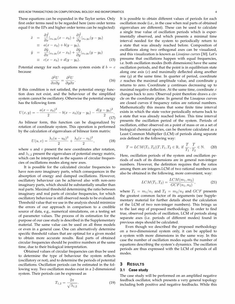
Dependence of periods on parameters β and γ for De-sign I is presented in Fig. 2. Values of other parameters areα = 50, ∆ = 10, σ = 1, n = 2 and m = 2. In Design I.1oscillations occur for extended range of parameters β andγ. The results of the analysis are presented in Fig. 3). Valuesof other parameters are α = 50 and ∆ = 4, σ = 1, n = 2and m = 2. The model of Design III also exhibits oscillatorybehaviour for a larger range of parameters β and γ thanDesign I as can be seen in Fig. 4. Values of other parametersare α = 50, ∆ = 1, σ = 1, n = 3 and m = 2.
IEEE/ACM TRANSACTIONS ON COMPUTATIONAL BIOLOGY AND BIOINFORMATICS 6
(a) (b) (c)
Fig. 1. Three different implementations of the amplified negative feedback oscillator that will be analysed, i.e. implementation with competitivebinding of repressor and activator at the activator promoter, namely Design I (a), a variation of Design I with competitive binding of repressor andactivator at the repressor promoter also, namely Design I.1 (b) and implementation without competition on either of promoters, namely Design III(c). Differences between the designs are emphasized.
(a) (b)
Fig. 2. Periods of oscillations in the model of Design I according to classical mechanics method (a) and numerical method (b), where α = 50,∆ = 10, σ = 1, n = 2 and m = 2. White colour denotes stationary behaviour.
4 CONCLUSION
Existing analytical methods are in general cases capableof answering the qualitative questions only, i.e., given theparameter values is the behaviour of the system understudy oscillatory or not. Recently, several analytical methodsfor quantitative analysis have been developed which canbe, however, applied only to limited oscillator topologies,and have a very limited biological relevance due to therough approximations they make in the process of modelsimplification. We introduced a general analytical methodthat is capable to respond with the qualitative and quanti-tative answer with an estimation of oscillation periods. Wedescribed a classical mechanics approach that can be usedfor the analysis of the oscillatory behaviour in biologicaloscillators modelled with the system of ordinary differentialequations. Proposed approach is based on the transforma-tion of an oscillator’s model to a classical mechanics system,more precisely to a harmonic oscillator. The methodologywas established to analyse the transformed system fromthe qualitative, i.e., is the behaviour oscillatory or static, as
well as from the quantitative perspective, i.e., what are theperiods of observed oscillations. The approach was verifiedon three different implementations of the amplified negativefeedback oscillator.
Proposed method is numerically stable while all mathe-matical operations performed in the analysis transform con-tinuous functions to continuous functions (except deriva-tion, which transforms smooth functions to continuousfunctions). This means that there is not any cause for di-vergence or instabilities related to parameters fluctuations ifinitial ODEs are smooth enough, which is always the casein the models in our focus.
Even though relatively accurate approximations of oscil-latory behaviour were obtained with the proposed method-ology, there is still some space for improvements. First of allwe need to have in mind that albeit numerical simulationsare treated as a reliable source, they may still producesome errors. Accuracy of the results of numerical analysisin [10], which was also adapted to our analysis, depends onchoice of appropriate amplitude fluctuation, which is chosen
IEEE/ACM TRANSACTIONS ON COMPUTATIONAL BIOLOGY AND BIOINFORMATICS 7
(a) (b)
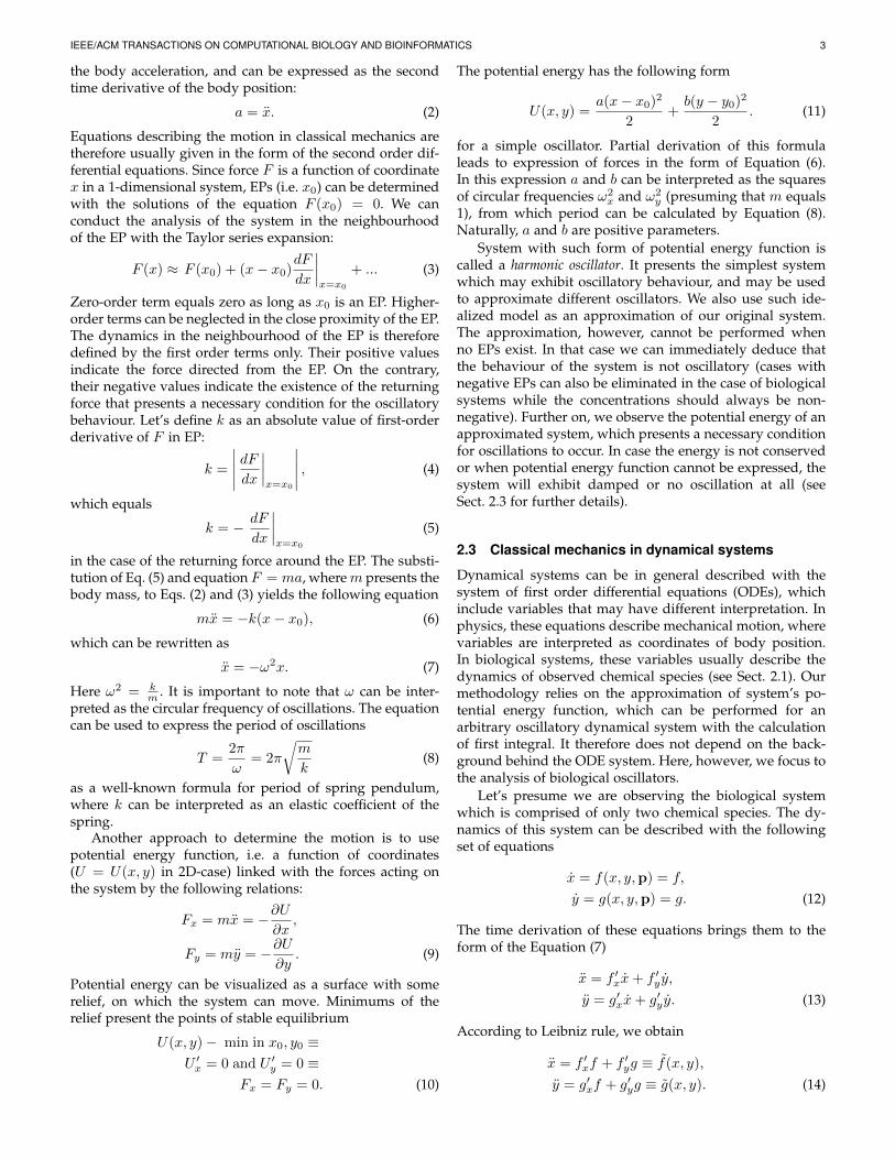
Fig. 3. Periods of oscillations in the model of Design I.1. according to classical mechanics method (a) and numerical method (b), where α = 50,∆ = 4, σ = 1, n = 2 and m = 2. White colour denotes stationary behaviour.
(a) (b)
Fig. 4. Periods of oscillations in the model of Design III according to classical mechanics method (a) and numerical method (b), where α = 50,∆ = 1, σ = 1, n = 3 and m = 2. White colour denotes stationary behaviour.
manually (according to supplementary code in [10] minimalamplitude equals 10−5). It is possible that smaller valueswould lead to the expansion of oscillatory regions. On theother hand, our approach may also introduce some errorsin the characterisation of oscillatory behaviour due to thelinearisation of a non-linear dynamical system.
Oscillatory behaviour is, however, also characterized byoscillation amplitudes, which are unfortunately not possibleto estimate with the proposed method. Oscillation ampli-tudes can be, on the other hand, determined with numericalsimulations. These can be conducted in a combination withproposed method, which can drastically reduce the parame-ter space on which numerical simulations are performed (i.e.simulations need to be performed only for parameter valuesthat result in oscillatory behaviour with certain oscillationperiods).
We end this discussion with some concrete biologicalapplications of proposed methodology. These can be foundin synthetic biology, i.e. for guiding the design of novel
biological oscillators, as well as in systems biology, i.e. forthe analysis of existing biological oscillators. For example,one can apply the proposed methodology to efficientlyanalyse different oscillator topologies before their experi-mental implementation. Methodology is able to efficientlyidentify the most robust topologies that also reflect desiredoscillation periods (in our case the most robust topology,i.e. the one with the largest oscillatory region, is Design I.1).Moreover, analysis conducted with proposed methodologycan guide the experimentalist to choose the components(e.g., promoters, ribosome binding sites, protein coding se-quences, etc.) with kinetic properties that match the param-eter values for which the desired behaviour is obtained. Lastbut not least, methodology can be applied in the analysis ofexisting biological oscillators. For example, it can be usedas a method behind the parameter estimation techniques toefficiently tune the modelled dynamics with experimentalresults describing the time-course of concentrations of oscil-latory species in the system under study.
IEEE/ACM TRANSACTIONS ON COMPUTATIONAL BIOLOGY AND BIOINFORMATICS 8
ACKNOWLEDGMENTS
The research was partially supported by the scientific-research programme Pervasive Computing (P2-0359) fi-nanced by the Slovenian Research Agency in the years from2009 to 2017 and by the basic research and applicationproject Designed cellular logic (J1-6740) financed by theSlovenian Research Agency in the years from 2014 to 2017.Results presented here are in scope of Ph.D. thesis that isbeing prepared by Anastasiia Vasylchenkova.
REFERENCES
[1] O. Purcell, N. J. Savery, C. S. Grierson, and M. di Bernardo, “Acomparative analysis of synthetic genetic oscillators,” Journal ofthe Royal Society Interface, vol. 7 (52), pp. 1503–1524, 2010.
[2] R. Guantes and J. F. Poyatos, “Dynamical principles of two-component genetic oscillators,” PLOS Computational Biology, vol. 2,pp. 0188–0197, 2006.
[3] J. C. Dunlap, “Molecular bases for circadian clocks,” Cell, vol. 96,pp. 271–290, 1999.
[4] J. J. Tyson, K. Chen, and B. Novak, “Network dynamics and cellphysiology,” Nature Reviews Molecular Cell Biology, vol. 2, pp. 908–916, 2001.
[5] M. B. Elowitz and S. Leibler, “A synthetic oscillatory network oftranscriptional regulators,” Nature, vol. 403, pp. 335–338, 2000.
[6] S. Muller, J. Hofbauer, L. Endler, C. Flamm, S. Widder, andP. Schuster, “A generalized model of the repressilator,” Journal ofMathematical Biology, vol. 53, pp. 905–937, 2006.
[7] O. Buse, R. Prez, and A. Kuznetsov, “Dynamical properties of therepressilator model,” Physical Review E, vol. 81, p. 066206, 2010.
[8] N. Strelkowa and M. Barahona, “Switchable genetic oscillator op-erating in quasi-stable mode,” Journal of the Royal Society Interface,vol. 7, pp. 1071–1082, 2010.
[9] B. Novak and J. J. Tyson, “Design principles of biochemical oscil-lators,” Nature Reviews Molecular Cell Biology, vol. 9, pp. 981–991,2008.
[10] A. Munteanu, M. Constante, M. Isalan, and R. Sole, “Avoidingtranscription factor competition at promoter level increases thechances of obtaining oscillation,” BMC Systems Biology, vol. 4,p. 66, 2010.
[11] S. H. Strogatz, Nonlinear Dynamics and Chaos: With Applications toPhysics, Biology, Chemistry, and Engineering, 2nd ed. WestviewPress, 2014.
[12] L. K. Nguyen, “Regulation of oscillation dynamics in biochemicalsystems with dual negative feedback loops,” J. R. Soc. Interface,vol. 9, pp. 1998–2010, 2012.
[13] N. Barkai and S. Leibler, “Circadian clocks limited by noise,”Nature, vol. 403, pp. 267–268, 2000.
[14] C. Kut, V. Golkhou, and J. S. Bader, “Analytical approximations forthe amplitude and period of a relaxation oscillator,” BMC SystemsBiology, vol. 3, 2009.
[15] K. Maeda and H. Kurata, “Analytical study of robustness of anegative feedback oscillator by multiparameter sensitivity,” BMCSystems Biology, vol. 8, 2014.
[16] B. C. Goodwin, “Oscillatory behavior in enzymatic control pro-cesses,” Advances in Enzyme Regulation, vol. 3, pp. 425–428, 1965.
[17] J. Stricker, S. Cookson, M. R. Bennett, W. H. Mather, L. S. Tsimring,and J. Hasty, “A fast, robust and tunable synthetic gene oscillator,”Nature, vol. 456, pp. 516–520, 2008.
[18] A. Caicedo-Casso, H.-W. Kang, S. Lim, and C. I. Hong, “Ro-bustness and period sensitivity analysis of minimal models forbiochemical oscillators,” Scientific Reports, vol. 5, 2015.
[19] S. M. Castillo-Hair, E. R. Villota, and A. M. Coronado, “Designprinciples for robust oscillatory behavior,” Systems and SyntheticBiology, vol. 9, pp. 125–133, 2015.
[20] T. Y.-C. Tsai, Y. S. Choi, W. Ma, J. R. Pomerening, C. Tang, and J. E.Ferrell Jr., “Robust, tunable biological oscillations from interlinkedpositive and negative feedback loops,” Science, vol. 321, pp. 126–129, 2008.
[21] T. Lebar, U. Bezeljak, A. Golob, M. Jerala, L. Kadunc, B. Pirs,M. Strazar, D. Vucko, U. Zupancic, M. Bencina, V. Forstneric,R. Gaber, J. Lonzaric, A. Majerle, A. Oblak, A. Smole, and R. Jerala,“A bistable genetic switch based on designable DNA-bindingdomains,” Nature Communications, 2014.
[22] Z. Zi, “Sensitivity analysis approaches applied to systems biologymodels,” IET Systems Biology, vol. 5, no. 6, pp. 336–346, 2011.
[23] N. Le Novere, “Quantitative and logic modelling of molecular andgene networks,” Nature Reviews Genetics, vol. 16, no. 3, pp. 146–158,2015.
[24] H. de Jong, “Modeling and simulation of genetic regulatory sys-tems: a literature review.” Journal of Computational Biology, vol. 9,no. 1, pp. 67–103, 2002.
[25] M. Kaern, W. J. Blake, and J. Collins, “The engineering of generegulatory networks,” Annu. Rev. Biomed. Eng., vol. 5, pp. 179–206,2003.
[26] U. Alon, An Introduction to Systems Biology. Chapman &Hall/CRC, 2007.
[27] H. M. Sauro, Enzyme Kinetics for Systems Biology. AmbrosiusPublishing, 2012.
[28] L. Bintu, N. E. Buchler, H. G. Garcia, U. Gerland, T. Hwa, J. Kon-dev, and R. Phillips, “Transcriptional regulation by the numbers:models,” Current opinion in genetics & development, vol. 15(2), pp.116–24, 2005.
[29] C. Kittel, W. D. Knight, M. A. Ruderman, A. C. Helmholz, and B. J.Moyer, Mechanics (Berkeley Physics Course, Vol. 1). McGraw-HillBook Company, 1973.
[30] V. Arnold, Mathematical Methods of Classical Mechanics, ser. Gradu-ate Texts in Mathematics. Springer, 1989.
[31] M. R. Atkinson, M. A. Savageau, J. T. Myers, and A. J. Ninfa,“Development of genetic circuitry exhibiting toggle switch oroscillatory behavior in escherichia coli,” Cell, vol. 113, pp. 597–607,2003.
[32] P. Smolen, D. A. Baxter, and J. H. Byrne, “Frequency selectivity,multistability, and oscillations emerge from models of geneticregulatory systems,” American Journal of Physiology, vol. 274, pp.C531–C542, 1998.
[33] M. Galassi, J. Davies, J. Theiler, B. Gough, G. Jungman, P. Alken,M. Booth, F. Rossi, and R. Ulerich, GNU Scientific Library: Referencemanual, 2013, edition 1.16.
Anastasiia Vasylchenkova is a postgraduatestudent at the V. N. Karazin Kharkiv NationalUniversity, Ukraine, Department of Physics andTechnologies. She received a BSc degree inApplied Physics in 2014. She has significantachievements in students physical tournaments.Her interests are dynamical systems, stochasticdynamics, classical and quantum chaos and hy-drodynamics and aerodynamics.
Miha Mraz received his BSc, MSc and PhDdegree in computer science from the Facultyof Computer and Information Science, Univer-sity of Ljubljana, Slovenia in 1992, 1995 and2000, where he leads the Computational biologygroup, and holds the position of a full professor.His research interests are unconventional pro-cessing methods, systems biology and syntheticbiology. He is a member of IEEE professionalsociety.
Nikolaj Zimic received his BSc, MSc and PhDdegree in computer science from the Faculty ofComputer and Information Science, Universityof Ljubljana, Slovenia in 1984, 1990 and 1994,where he holds the position of a full professor.His research interests are in the fields of uncon-ventional computing, fuzzy logic and computernetworks. He is a member of IEEE professionalsociety.
Miha Moskon received his BSc and PhD de-gree in computer science from the Faculty ofComputer and Information Science, Universityof Ljubljana, Slovenia in 2007 and 2012, wherehe holds the position of an assistant professor.His main research interests are directed towardsquantitative modelling and analysis of gene reg-ulatory networks and towards computational de-sign of synthetic biological systems. He is es-pecially interested in biological oscillators, theirapplications and analysis.
All the models described presume that the protein binding and mRNA dynamicsare much faster than the protein translation and degradation and were obtainedin the same way as described in [1, 2]. We give a more detailed derivation ofthese models in the following sections.
1.1 Design I
Design I presents the topology, in which activator and repressor compete forthe same binding sites on the activator promoter. They bind to the promoterin multimerised form and multimerisation can be considered as a single stepreaction with the Hill aproximation. Binding and multimerisation reactions canbe thus described as follows:
PR +Ank1k−1
PRAn,
PA +Rmk2k−2
PARm,
PA +Ank3k−3
PAAn.
1
mRk5k−5
Rm,
nAk6k−6
An,
Here R represents repressor protein, Rm repressor multimer, A activator protein,An activator multimer, PR repressor promoter, PRAn activated repressor pro-moter, PA activator promoter, PARm repressed activator promoter and PAAnactivated activator promoter.
Transcription, translation and degradation reactions can be described in thefollowing way:
PRβR→PR +mR,
PRAnαβR→ PRAn +mR,
PAβA→PA +mA,
PAAnαβA→ PAAn +mA,
mRγR→mR +R,
mAγA→mA +A,
mRαR→0,
mAαA→0,
RδR→0,
AδA→0.
Here mR represents repressor mRNA and mA represents activator mRNA.Since binding and multimerisation reactions occur in a much faster timescale
than transcription, translation and degradation, they can be assumed to be inequilibrium.
Repressor promoter can be in two different states in Design I topology, i.e.unoccupied (PR) or activated (PRAn). Weights of these states can be expressedin the following way:
W (PR) = 1,
W (PRAn) = K1KAAn,
where A denotes the concentration of activator protein, K1 = k1k−1
and KA =k6k−6
.
Probability of each promoter state can be calculated with the fractionaloccupancy approach [3] applying the weights in the following equation:
p(si) =W (si)k∑j=1
W (sj)
,
2
where k is the number of all possible states. In our case probabilities are
p(PR) =1
1 +K1KAAn,
p(PRAn) =K1KAA
n
1 +K1KAAn.
The rate of repressor mRNA transcription thus equals
PTRβR1 + αK1KAA
n
1 +K1KAAn,
where PTR is the total concentration of repressor promoter.Transcription rate of activator mRNA can be expressed in a similar way.
Activator promoter can be in three different states in Design I topology, i.e.unoccupied (PA), repressed (PARm) or activated (PAAn). Weights of thesestates can be expressed as
W (PA) = 1,
W (PARm) = K2KRRm,
W (PAAn) = K3KAAn,
where R denotes the concentration of repressor protein, K2 = k2k−2
, K3 = k3k−3
and KR = k5k−5
. State probabilities are thus
p(PA) =1
1 +K2KRRm +K3KAAn,
p(PARm) =K2KRR
m
1 +K2KRRm +K3KAAn,
p(PAAn) =K3KAA
n
1 +K2KRRm +K3KAAn
and transcription rate of activator mRNA
PTAβA1 + αK3KAA
n
1 +K2KRRm +K3KAAn,
where PTA is the total concentration of activator promoter.Combining the transcription rates with the mRNA degradation yields the
following differential equations governing the dynamics of mRNA species:
dmR
dt= βRP
TR
1 + αK1KAAn
1 +K1KAAn− αRmR,
dmA
dt= βAP
TA
1 + αK3KAAn
1 +K2KRRm +K3KAAn− αAmA,
3
where mR and mA denote the concentrations of repressor and activator mRNA.Activator and repressor dynamics governed by translation and degradation canbe described with two additional differential equations:
dR
dt= γRmR − δRR,
dA
dt= γAmA − δAA.
These equations can be simplified with the quasi-steady-state approximation,i.e. dmR
dt ≈ 0 and dma
dt ≈ 0 [1], which yields the following model:
dR
dt= γR
βRαR
PTR1 + αK1KAA
n
1 +K1KAAn− δRR,
dA
dt= γA
βAαA
PTA1 + αK3KAA
n
1 +K2KRRm +K3KAAn− δAA.
1.2 Design I.1
Variation of Design I (Design I.1) includes a binding site for repressor on its ownpromoter. It can be modelled with an additional state of repressor promoter,i.e. PRRm, for which the transcription rate is assumed to be zero. The rate ofrepressor mRNA transcription thus equals
PTRβR1 + αK1KAA
n
1 +K1KAAn +K4KRRm,
where K4 = k4k−4
, and k4 and k−4 describe the on-rate and the off-rate constants
of the repressor and its promoter binding. The rest of the model can be derivedin the same way as for Design I and can be described as
dR
dt= γR
βRαR
PTR1 + αK1KAA
n
1 +K1KAAn +K4KRRm− δRR,
dA
dt= γA
βAαA
PTA1 + αK3KAA
n
1 +K2KRRm +K3KAAn− δAA.
1.3 Design III
Design III implementation includes separate binding sites for activator and re-pressor on the activator promoter. The adaptation of Design I to Design IIImodel is again straightforward. We need to regard additional state of activatorpromoter, i.e. PARmAn, for which the transcription rate is again assumed tobe zero. The rate of activator mRNA transcription thus equals:
PTA1 + αK3KAA
n
1 +K2KRRm +K3KAAn +K2KRRmK3KAAn.
4
Again, the same procedure as in Design I can be followed in the rest of thederivation. It brings us to the following model:
dR
dt= γR
βRαR
PTR1 + αK1KAA
n
1 +K1KAAn− δRR,
dA
dt= γA
βAαA
PTA1 + αK3KAA
n
1 +K2KRRm +K3KAAn +K2KRRmK3KAAn− δAA.
1.4 Rescaling the variables
Transformation to the models presented in the main text can be achieved byrescaling all variables to become dimensionless [1, 2]:
x = n√K3KAA,
y = m√K3KAR,
τ = tδR,
∆ =δAδR,
β =γAβAδAαA
PTAn√K3KA,
γ =γRβRδRαR
PTRm√K3KA,
σ =K2KR
K3KA.
1.5 Parameter values
The nominal parameter values used in our analysis were obtained from theliterature [1, 2] and are as follows:
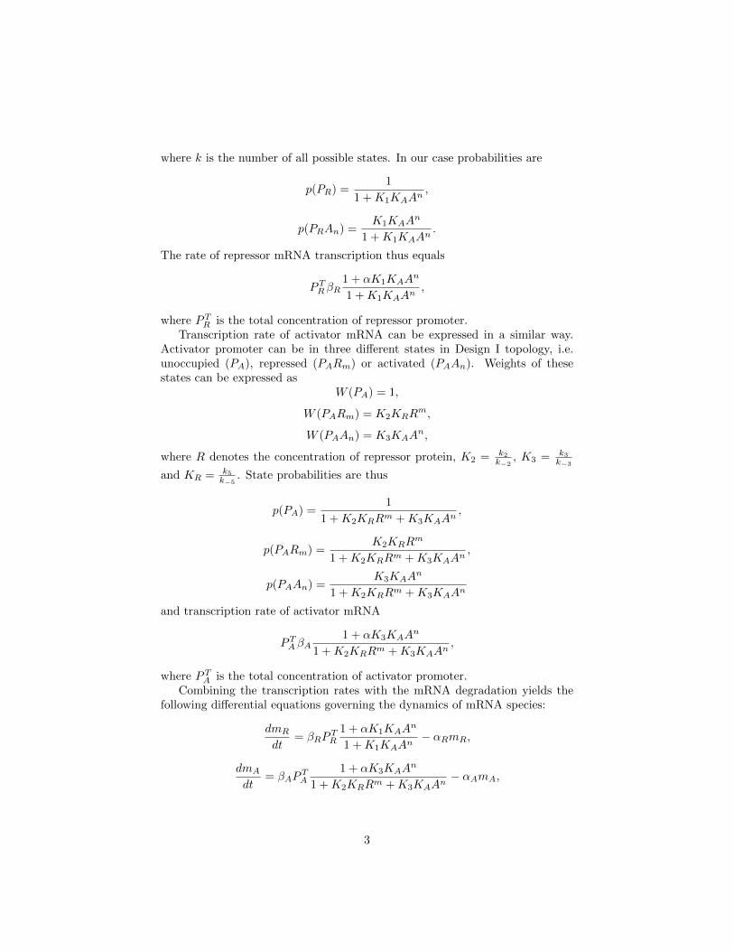
Figure 1: Comparison of the non-linearity of promoter response approximationbetween biological plausible scenarios (e.g., n=1, n=2 or n=4) and approachusing Heaviside or unit-step function.
• γR = 0.1 · γA,
• δA = 1h−1,
• δR = 0.1h−1,
• PTA = PTR = 1.
2 Using unit step function to approximate pro-moter activity
Approaches described in [4] and [5] rely on the approximation of a promoteractivity with a Boolean variable with only two possible values, i.e. zero (notactive) and one (active), using unit step function as θ (A−KdA) for activationand θ (KdR −R) for repression. Here KdA and KdR present the dissociationconstants that can be interpreted as transcription factor concentrations produc-ing half occupation of the promoter. This approximations yield a very highnon-linearity of promoter response, which is often not plausible. For example,the model we used in our case study presumes the Hill coefficients equal to 2 or3, which generates a response that is far from unit step function (see Fig. 1).
We can be still apply this approximation to the amplified negative feed-back oscillator models described in previous section. In this case dissociation
6
lg β-2 0 2 4
lg γ
-2
-1
0
1
2
3
4lg T
4.6
4.8
5
5.2
Figure 2: Oscillation periods obtained on the unit step function model of DesignI and Design III implementation of an amplified negative feedback oscillator.
constants can be expressed as
KdA = n
√1
K1KA,
KdR = m
√1
K2KR.
For example, Design I and Design III models can be adapted to
dR
dt= γR
βRαR
PTR (θ (KdA −A) + αθ (A−KdA))− δRR,
dA
dt= γA
βAαA
PTA θ (KdR −R) (θ (KdA −A) + αθ (A−KdA))− δAA.
Note that this modelling approach is due to the simplification with a unit stepfunction unable to differ among Design I and Design III implementation. Resultsof previous analyses however indicate that substantial differences in the dynam-ics of these two topologies exist. We performed the analysis on the simplifiedmodel with the same parameter values as described in the main text. Modelyielded solutions that were hardly comparable to the results of non-simplifiedmodels (see Fig. 2). We can conclude that the unit step function approxima-tion can be applied only to a limited scope of biological systems and has a verylimited biological relevance.
7
3 Calculation of the LCM of real numbers
Here we demonstrate that the LCM of two numbers A and B can be obtainedfrom the formula
LCM(A,B) =LCM(m1,m2)
GCF (n1, n2), (1)
where GCM stands for the greatest common multiplier. If A and B are ra-tional numbers (according to limited numerical accuracy we are always dealingwith rational numbers in computational calculations) it means that they can beexpressed in the form A = m1/n1 and B = m2/n2, which brings us to relation
LCM(A,B)
A=
LCM(m1,m2)
m1· n1GCF (n1, n2)
= integer · integer = integer. (2)
4 Evaluating the threshold values
Oscillatory behavior is sometimes achieved also with non-zero imaginary partsof calculated circular frequencies, which should be however substantially smallerthan real parts. Threshold values that we use in the analysis should minimizethe errors of our approach in comparison to a credible source of data, e.g.,numerical simulations, on a testing set of parameter values. Percentage errorcan be quantified with the following measure:
E =ncnT· 100%, (3)
where nc presents the number of conflict points and nT the total number ofpoints on which evaluation is performed. Note that the denominator uses thetotal number of points, while even numerical simulations cannot be consideredas an absolutely accurate method. Fig. 3 presents the values of E in dependenceon the threshold value for Design I. Threshold value in which E is minimizedwas used for period estimation in the main paper. The same value can be usedon all three models or even in a general case. One can alternatively determinespecific threshold values that are optimal for a given model to obtain moreaccurate results.
References
[1] R. Guantes and J. F. Poyatos, “Dynamical principles of two-componentgenetic oscillators,” PLOS Computational Biology, vol. 2, pp. 0188–0197,2006.
[2] A. Munteanu, M. Constante, M. Isalan, and R. Sole, “Avoiding transcrip-tion factor competition at promoter level increases the chances of obtainingoscillation,” BMC Systems Biology, vol. 4, p. 66, 2010.
8
Figure 3: Effect of threshold values on the error introduced by classical mechan-ics approach in comparison to numerical simulations for Design I model.
[3] H. M. Sauro, Enzyme Kinetics for Systems Biology. Ambrosius Publishing,2012.
[4] C. Kut, V. Golkhou, and J. S. Bader, “Analytical approximations for theamplitude and period of a relaxation oscillator,” BMC Systems Biology,vol. 3, 2009.
[5] K. Maeda and H. Kurata, “Analytical study of robustness of a negativefeedback oscillator by multiparameter sensitivity,” BMC Systems Biology,vol. 8, 2014.


![[Kibble] - Classical Mechanics](https://static.documents.pub/doc/80x56/552056344a79596f718b4715/kibble-classical-mechanics.jpg)


![Classical Mechanics - people.phys.ethz.chdelducav/cmscript.pdf · References [1]LandauandLifshitz,Mechanics,CourseofTheoreticalPhysicsVol.1., PergamonPress [2]Classical Mechanics,](https://static.documents.pub/doc/80x56/5e1e9832bac1ea74484e9601/classical-mechanics-delducavcmscriptpdf-references-1landauandlifshitzmechanicscourseoftheoreticalphysicsvol1.jpg)


