Classical Mechanics - German Research School for ... · Emiliano Ippoliti Review 2 Physics •...

From Molecular to Con/nuum Physics I WS 11/12Emiliano Ippoli/| October, 2011

Classical Mechanics

Wednesday, October 12, 2011

Emiliano Ippoliti

Review

2

Physics • Basic thermodynamics • Temperature, ideal gas, kinetic gas theory, laws of thermodynamics • Statistical thermodynamics • Canonical ensemble, Boltzmann statistics, partition functions, internal and free energy, entropy • Basic electrostatics • Classical mechanics • Newtonian, Lagrangian, Hamiltonian mechanics • Quantum mechanics • Wave mechanics • Wave function and Born probability interpretation • Schrödinger equation • Simple systems for which there is an analytical solution • Free particle • Particle in a box, particle on a ring • Rigid rotator • Harmonic oscillator • Basics • Uncertainty relation • Operators and expectation values • Angular momentum • Hydrogen atom • Energy values, atomic orbitals • Electron spin • Quantum mechanics of several particles (Pauli principle) • Many electron atoms • Periodic system: structural principle • Molecules • Two-atomic molecules (H2+,H2, X2) • Many-atomic molecules

Chemistry...

Informatics...

Mathematics...


Emiliano Ippoliti

Review

3

Physics • Basic thermodynamics • Temperature, ideal gas, kinetic gas theory, laws of thermodynamics • Statistical thermodynamics • Canonical ensemble, Boltzmann statistics, partition functions, internal and free energy, entropy • Basic electrostatics • Classical mechanics • Newtonian, Lagrangian, Hamiltonian mechanics • Quantum mechanics • Wave mechanics • Wave function and Born probability interpretation • Schrödinger equation • Simple systems for which there is an analytical solution • Free particle • Particle in a box, particle on a ring • Rigid rotator • Harmonic oscillator • Basics • Uncertainty relation • Operators and expectation values • Angular momentum • Hydrogen atom • Energy values, atomic orbitals • Electron spin • Quantum mechanics of several particles (Pauli principle) • Many electron atoms • Periodic system: structural principle • Molecules • Two-atomic molecules (H2+,H2, X2) • Many-atomic molecules

Chemistry...

Informatics...

Mathematics...


Emiliano Ippoliti

Classical Mechanics

4

• In Mechanics one examines the laws that govern the motion of bodies of matter. • Under motion one understands a change of place as a function of time.

• The motion happens under the influence of forces, that are assumed to be known.


Emiliano Ippoliti

Fundamentalelements

5

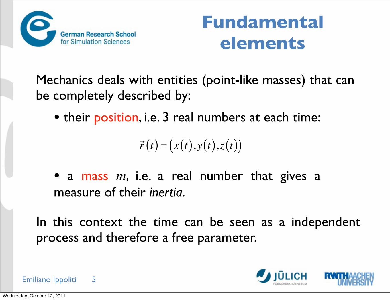
Mechanics deals with entities (point-like masses) that can be completely described by:

• their position, i.e. 3 real numbers at each time:

• a mass m, i.e. a real number that gives a measure of their inertia.

r t( ) = x t( ), y t( ), z t( )( )

In this context the time can be seen as a independent process and therefore a free parameter.


Emiliano Ippoliti

Some definitions

6

The velocity is given by

r t( ) = drdt

The acceleration is defined by

r t( ) = d 2rdt 2

=drdt


Emiliano Ippoliti

Newtonian Mechanics

7

Newton, Isaac (1643-1727)


Emiliano Ippoliti

Inertial frames

8

To write down the equations of motion for a certain problem, one first has to choose a frame of reference. The goal is then to find a frame of reference in which the lawsof mechanics take their simplest form.

It can be derived that one can always find a frame of reference in which space is homogeneous and isotropic and time is homogeneous. This is then called an ”inertial frame”. In such a frame a free body which is at rest at some instant of time always remains at rest. The same is true if the body moves with a velocity constant in both magnitude and direction. This is the Newton’s First Law.


Emiliano Ippoliti 9

Galileo’s Relativity Principle

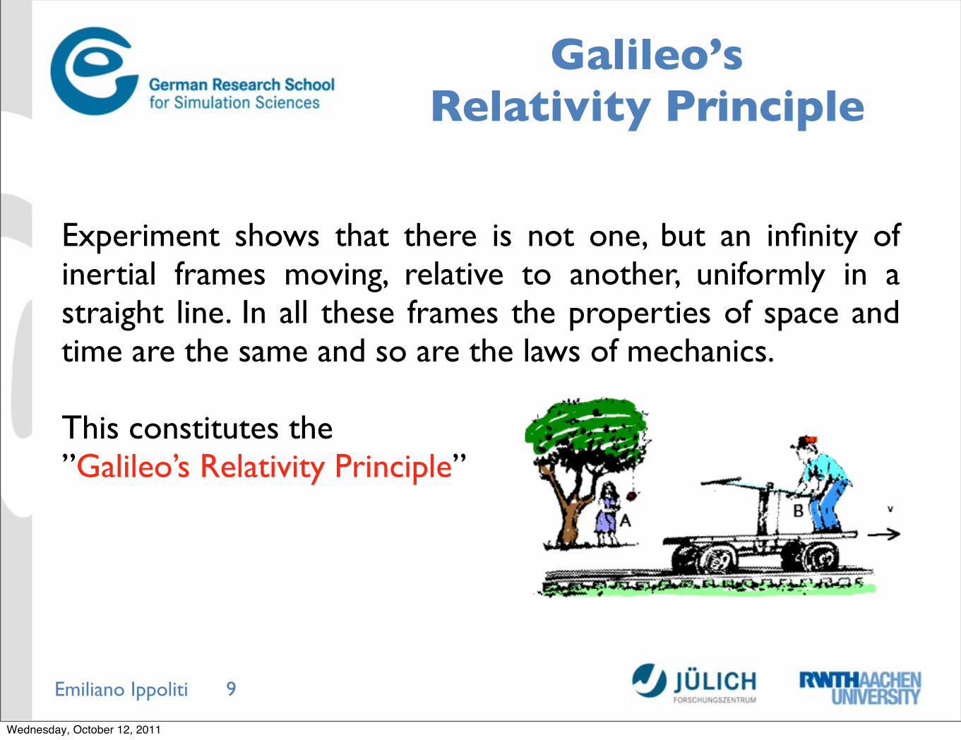
Experiment shows that there is not one, but an infinity of inertial frames moving, relative to another, uniformly in a straight line. In all these frames the properties of space and time are the same and so are the laws of mechanics.

This constitutes the”Galileo’s Relativity Principle”


Emiliano Ippoliti

Forces

10

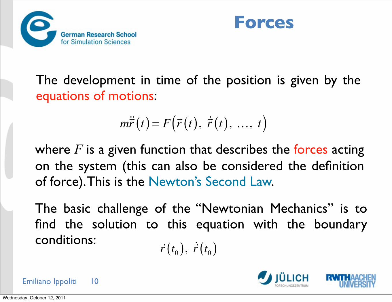
The development in time of the position is given by the equations of motions:

mr t( ) = F r t( ), r t( ), …, t( )

where F is a given function that describes the forces acting on the system (this can also be considered the definition of force). This is the Newton’s Second Law.

The basic challenge of the “Newtonian Mechanics” is to find the solution to this equation with the boundary conditions:

r t0( ), r t0( )


Emiliano Ippoliti

PotentialEnergy

11

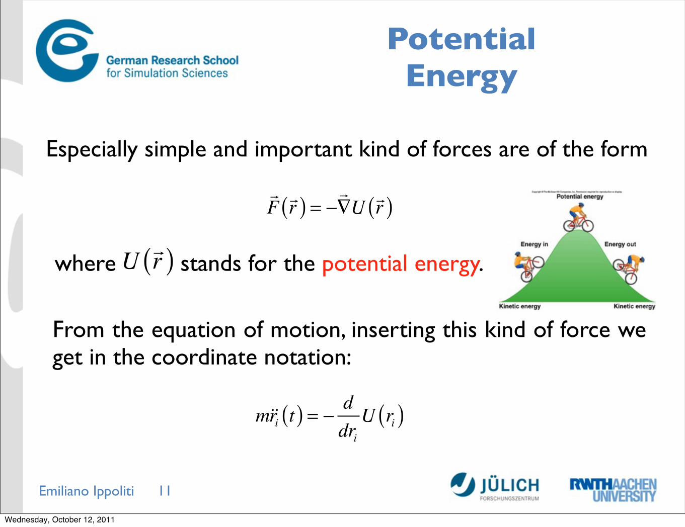
Especially simple and important kind of forces are of the form

F r( ) = −

∇U r( )

where stands for the potential energy. Ur( )

From the equation of motion, inserting this kind of force we get in the coordinate notation:

mri t( ) = −

ddriU ri( )


Emiliano Ippoliti

Motion constant:Total Energy

12

Taking the scalar product with this becomes ri t( )

mri t( ) ri t( ) = −

dridt

ddriV ri( )

Using the derivative chain rule:

ddt

mri t( )2( ) = 2mriri ddtU ri t( )( ) = dU

drii∑ dri

dt

we can rewrite our equation as the total differential

ddt

12mr 2 t( ) +U r t( )( )⎛

⎝⎜⎞⎠⎟= 0

Kinetic Energy


Emiliano Ippoliti

Lagrangian Mechanics

13

Lagrange, Joseph (1736-1813)


Emiliano Ippoliti

Principle of Least Action

14

Let the mechanical (n particles) system fulfill the boundary conditions

ra t1( ) = ra1

ra t2( ) = ra2Then, the condition on the system is that it moves between these positions in such a way that the integral

S = L

r1,r2 ,…, r1,

r2 ,…,t( )dtt1

t2∫is minimized. S is called the action and L is the Lagrangian associated with the given system.


Emiliano Ippoliti

Lagrange’sEquations

15

Using the variational calculus it can be proved that minimizing the action is equivalent to solve the system of 3n second-order differential equations:

ddt

∂L∂ra

⎛⎝⎜

⎞⎠⎟−∂L∂ra

= 0 a = 1,…,n

These are the ”Lagrange’s Equations” and are the equations of motion of the system (they give the relations between acceleration, velocities and coordinates). The general solution contains 6n constants, which can be determined from the initial conditions of the system (e.g. initial values of coordinates and velocities).


Emiliano Ippoliti

Uniqueness

16

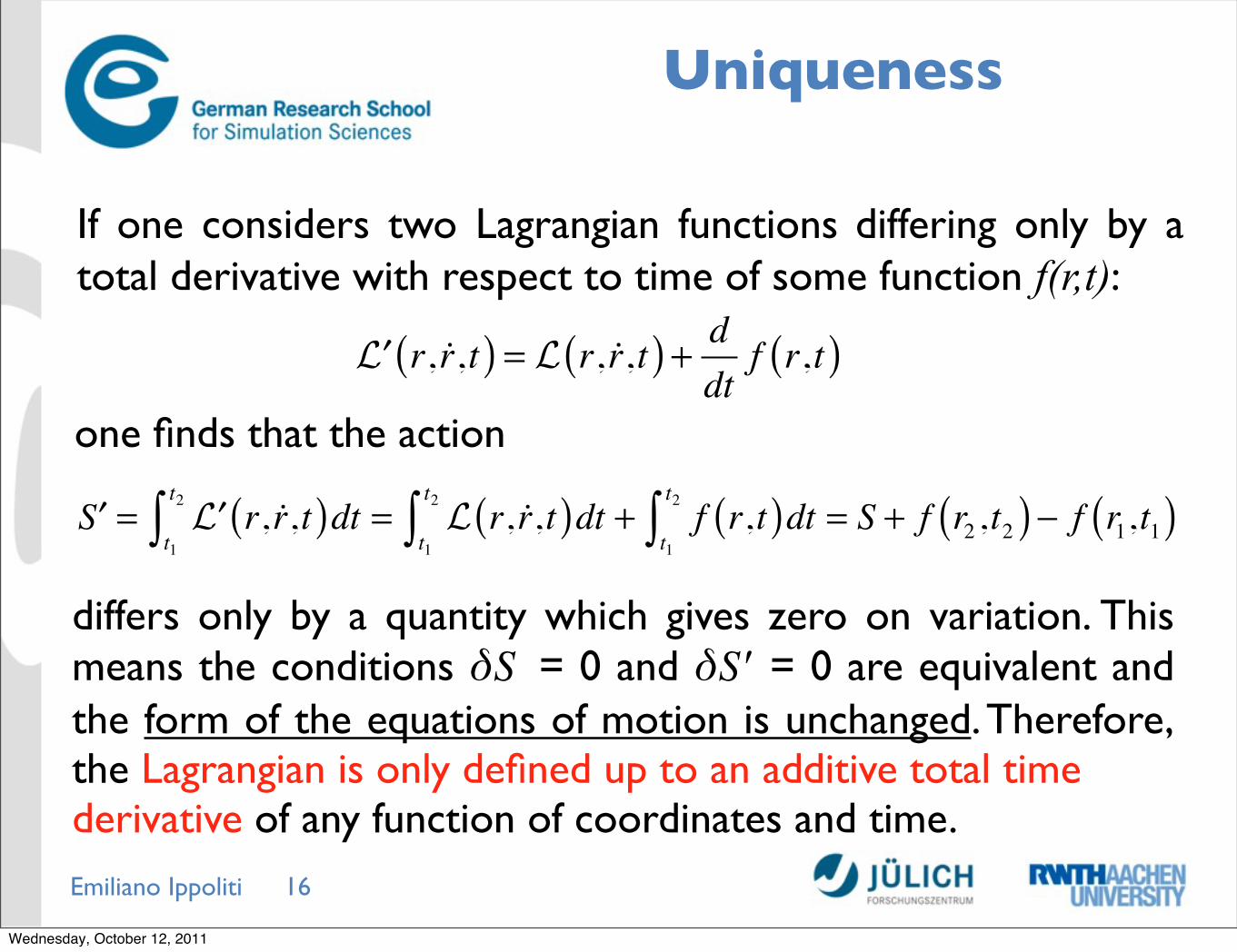
If one considers two Lagrangian functions differing only by a total derivative with respect to time of some function f(r,t):

′L r, r,t( ) = L r, r,t( ) + d

dtf r,t( )

one finds that the action

′S = ′L r, r,t( )dt

t1

t2∫ = L r, r,t( )dtt1

t2∫ + f r,t( )dtt1

t2∫ = S + f r2 ,t2( ) − f r1,t1( )

differs only by a quantity which gives zero on variation. This means the conditions δS = 0 and δS′ = 0 are equivalent and the form of the equations of motion is unchanged. Therefore, the Lagrangian is only defined up to an additive total timederivative of any function of coordinates and time.


Emiliano Ippoliti

Lagrangian of a free particle

17

The Lagrangian associated to a system has to have the same symmetry properties of the system itself:

- In a free particle system the space is homogeneous

L cannot depend explicitly on the vector position

r

- In a free particle system the time is homogeneous

L cannot depend explicitly on the time t

- In a free particle system the space is isotropic

L cannot depend on the direction of the vector velocity

r

dLdt

= 0 ⇒ L = Lr , r( )

dLdr

= 0 ⇒ L = Lr( )

L = Lr 2( ) = L

v 2( ) = L v2( )


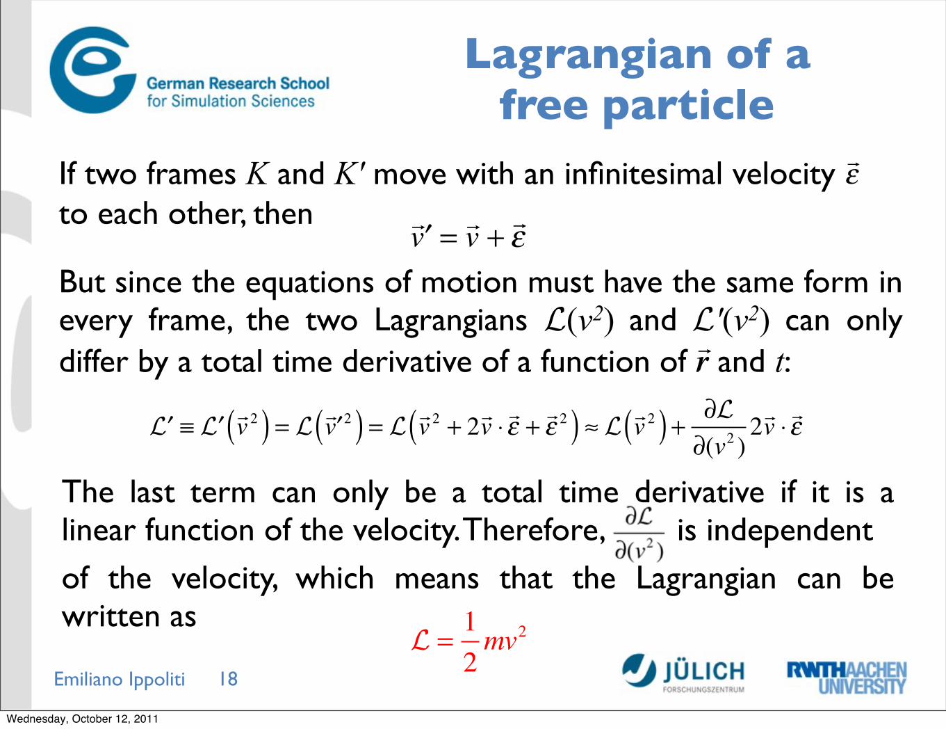
Emiliano Ippoliti 18

Lagrangian of a free particle

′L ≡ ′L

v 2( ) = L′v 2( ) = L

v 2 + 2v ⋅ ε + ε 2( ) ≈ Lv 2( ) + ∂L

∂(v2 )2v ⋅ ε

If two frames K and K′ move with an infinitesimal velocity to each other, then

ε

′v = v + ε

But since the equations of motion must have the same form in every frame, the two Lagrangians L(v2) and L′(v2) can only differ by a total time derivative of a function of r and t:

The last term can only be a total time derivative if it is a linear function of the velocity. Therefore, is independentof the velocity, which means that the Lagrangian can be written as

L =

12mv2

r


Emiliano Ippoliti

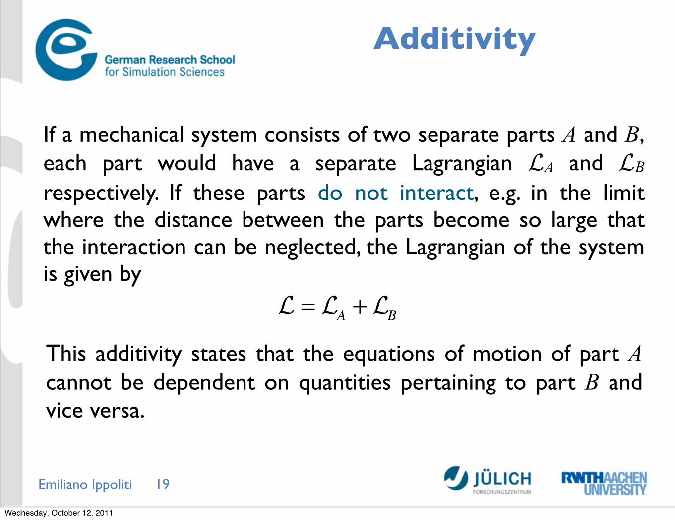
Additivity

19

If a mechanical system consists of two separate parts A and B, each part would have a separate Lagrangian LA and LB

respectively. If these parts do not interact, e.g. in the limit where the distance between the parts become so large that the interaction can be neglected, the Lagrangian of the system is given by

L = LA +LB

This additivity states that the equations of motion of part A cannot be dependent on quantities pertaining to part B and vice versa.


Emiliano Ippoliti

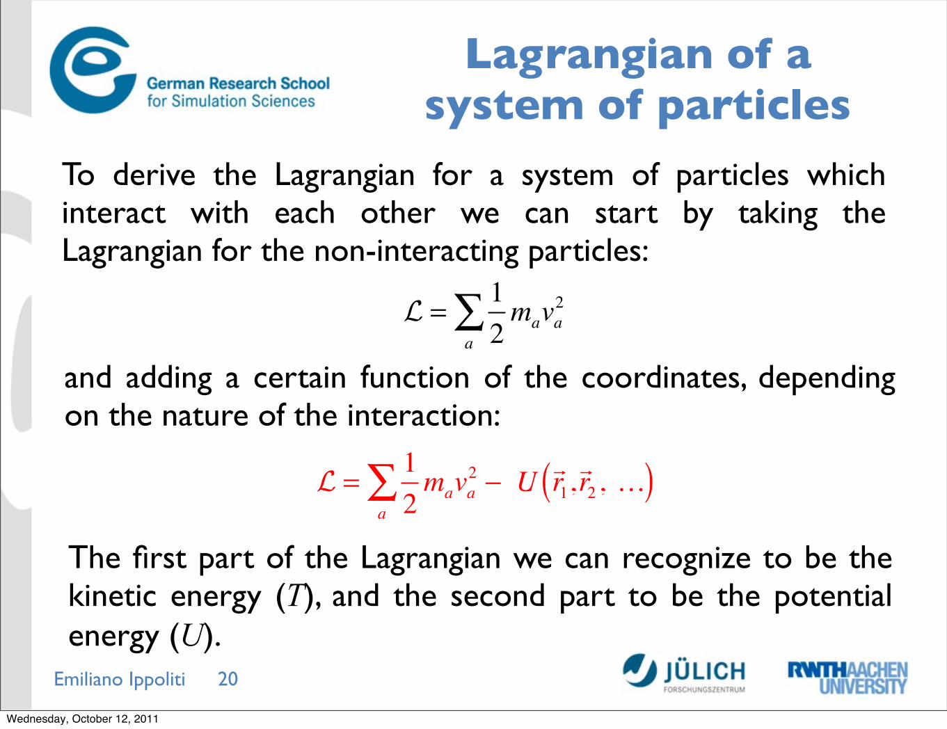
Lagrangian of a system of particles

20

To derive the Lagrangian for a system of particles which interact with each other we can start by taking the Lagrangian for the non-interacting particles:

and adding a certain function of the coordinates, depending on the nature of the interaction:

L =

12mava

2

a∑

L =

12mava

2

a∑ − U r1,

r2 , …( )The first part of the Lagrangian we can recognize to be the kinetic energy (T), and the second part to be the potential energy (U).


Emiliano Ippoliti

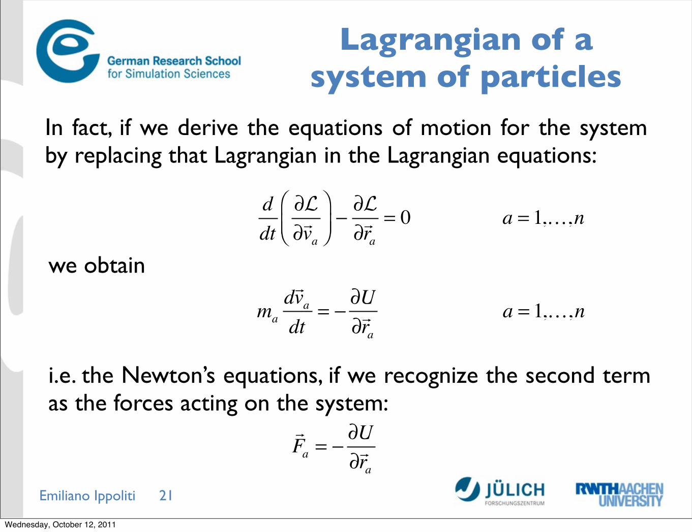
Lagrangian of a system of particles

21

In fact, if we derive the equations of motion for the system by replacing that Lagrangian in the Lagrangian equations:

ddt

∂L∂va

⎛⎝⎜

⎞⎠⎟−∂L∂ra

= 0 a = 1,…,n

we obtain

ma

dvadt

= −∂U∂ra

a = 1,…,n

i.e. the Newton’s equations, if we recognize the second term as the forces acting on the system:

Fa = −

∂U∂ra


Emiliano Ippoliti

When Lagrangian Mechanics

22

It is often necessary to deal with mechanical systems in which the interactions between different bodies take the form of constraints. These constraints can be very complicated and hard to incorporate, when working directly with the differential equations of motion.

Here it is often eas ier to construct a Lagrange function out of the kinetic and potential energy of the system and derive the correct equations of motion from there.


Emiliano Ippoliti

Hamiltonian Mechanics

23

Hamilton, William Rowan (1805–1865)


Emiliano Ippoliti

Generalized coordinates

24

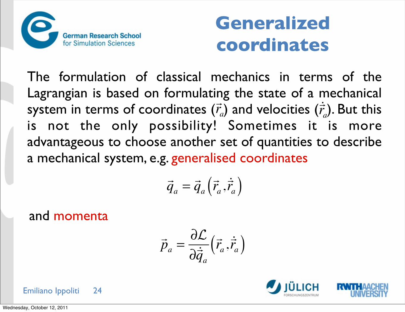
The formulation of classical mechanics in terms of the Lagrangian is based on formulating the state of a mechanical system in terms of coordinates ( ) and velocities ( ). But this is not the only possibility! Sometimes it is more advantageous to choose another set of quantities to describe a mechanical system, e.g. generalised coordinates

ra

and momenta

ra

qa =qara ,ra( )

pa =∂L∂qara ,ra( )


Emiliano Ippoliti

Legendre transformation

25

Then the total differential of the Lagrangian is given by

dL =

∂L∂qa

dqaa∑ +

∂L∂qa

dqaa∑ = pad

qaa∑ + pad

qaa∑

From the Lagrangian equation:

ddt

∂L∂qa

⎛⎝⎜

⎞⎠⎟−∂L∂qa

= 0 ⇒∂L∂qa

=dpadt

= pa

Using the differential chain rule applied on the last term

dL = pad

qaa∑ + d pa

qa( )a∑ − qad

paa∑


Emiliano Ippoliti

Hamiltonian

26

Rearranging this we end up with

d pa

qaa∑ −L

⎛⎝⎜

⎞⎠⎟= − pad

qaa∑ + qad

paa∑

the argument of the total differential on the left side is the total energy of the conservative system (T+U), now only expressed in terms of coordinates and momenta. In this form we call it the ”Hamiltonian” or ”Hamilton’s function” of the system:

Hq, p,t( ) = pa

qaa∑ −L

qa∂L∂qaa

∑ = paqa

a∑ = 2T

Since the L = T - U and we can write (using Euler’s theorem on homogeneous functions):


Emiliano Ippoliti

Hamilton’s equations

27

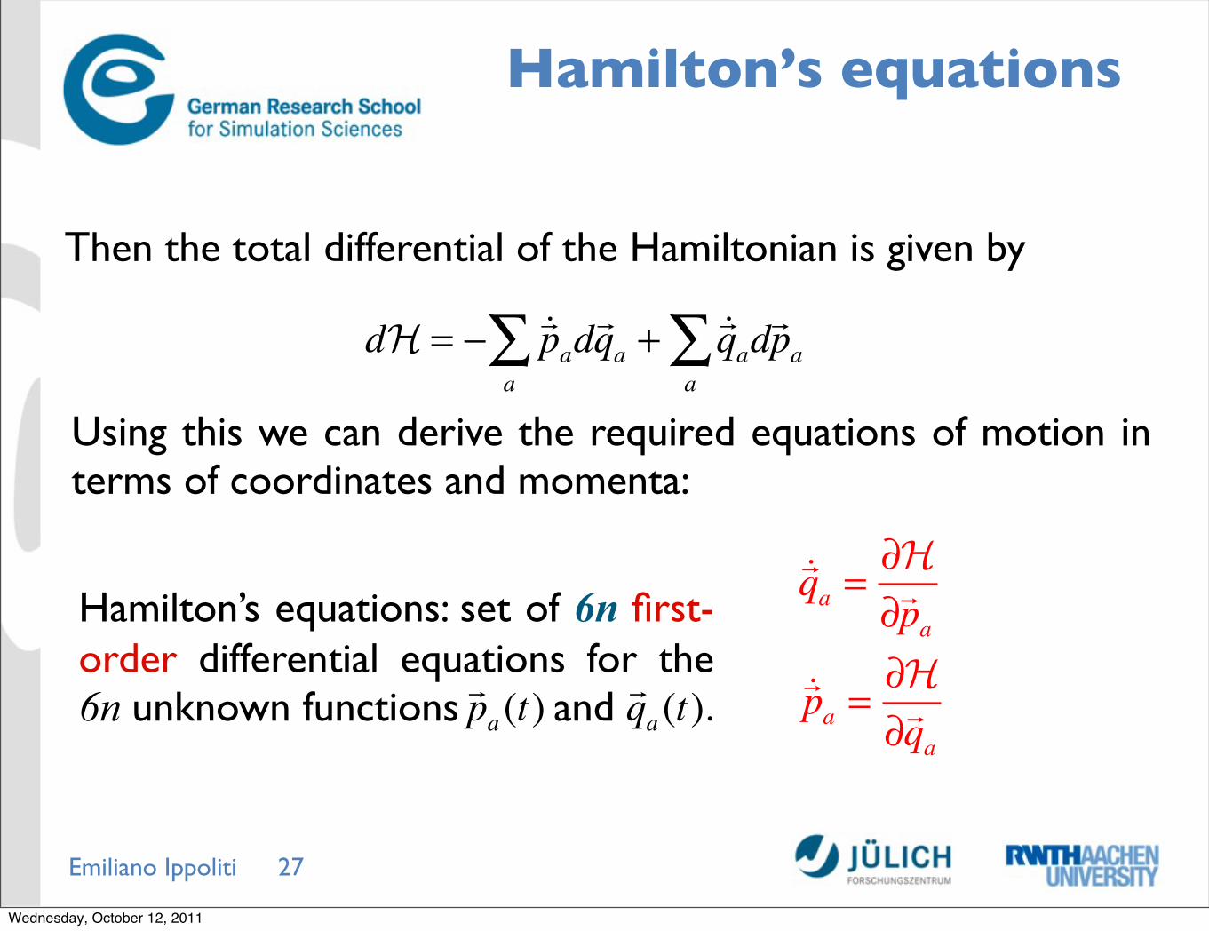
Then the total differential of the Hamiltonian is given by

dH = − pad

qaa∑ + qad

paa∑

Using this we can derive the required equations of motion in terms of coordinates and momenta:

qa =∂H∂pa

pa =∂H∂qa

Hamilton’s equations: set of 6n first-order differential equations for the 6n unknown functions and

pa (t) qa (t).


Emiliano Ippoliti

Lagrange vs Hamilton

28

The difference between the Lagrangian and Hamiltonian formalism is only a Legendre transformation. For some problems it is easier to write L down, for others H.

One is given by a system of 3n second-order differential equations, while the other one describes the same physical problem with 6n first-order differential equations.


Emiliano Ippoliti

Summarizing

29

Newtonianmechanics

Lagrangianmechanics

Hamiltonianmechanics

SystemForces Lagrangian Hamiltonian

Equations of motion

Type of mathematical

problem

3n second(or more)-order differential equations

3n second-order differential equations

6n first-order differential equations

L = Lra ,ra ,t( ) H = H

qa ,pa ,t( )

Fa =

Fara ,ra ,ra ,...,t( )

Fa = ma

ra

ddt

∂L∂ra

⎛⎝⎜

⎞⎠⎟−∂L∂ra

= 0

(a = 1,…,n)

(a = 1,…,n)

qa =∂H∂pa

pa =∂H∂qa


Emiliano Ippoliti

Venn diagram

30

Under some assumptions, we can represent the sets of the systems that can be described by Newtonian (N), Lagrangian (L) and Hamiltonian (H) mechanics this way:

N L H


Emiliano Ippoliti

References

31

1. M. Ganz. Introduction to Lagrangian and Hamiltonian Mechanics. http://image.diku.dk/ganz/Lectures/Lagrange.pdf

2. H. Goldstein. Classical mechanics. Addison-Wesley, Cambridge, 1950.

3. L.D. Landau and E.M. Lifschitz. Mechanics. Butterworth, Oxford, 1981.


Date post:	03-Aug-2018
Category:	Documents
Upload:	dongoc
View:	221 times
Download:	0 times

Classical Mechanics - German Research School for ... · Emiliano Ippoliti Review 2 Physics •...

Documents