1

Classical Multidimensional Scaling: A SubspacePerspective, Over-Denoising and Outlier Detection

Lingchen Kong, Chuanqi Qi and Hou-Duo Qi

Abstract—The classical Multi-Dimensional Scaling (cMDS) hasbecome a cornerstone for analyzing metric dissimilarity data dueto its simplicity in derivation, low computational complexity andits nice interpretation via the principle component analysis. Thispaper focuses on its capability of denoising and outlier detection.Our new interpretation shows that cMDS always overly denoisesa sparsely perturbed data by subtracting a fully dense denoisingmatrix in a subspace from the given data matrix. This leads usto consider two types of sparsity-driven models: Subspace sparseMDS and Full-space sparse MDS, which respectively uses the`1 and `1−2 regularization to induce sparsity. We then developfast majorization algorithms for both models and establish theirconvergence. In particular, we are able to control the sparsitylevel at every iterate provided that the sparsity control parameteris above a computable threshold. This is a desirable property thathas not been enjoyed by any of existing sparse MDS methods.Our numerical experiments on both artificial and real datademonstrates that cMDS with appropriate regularization canperform the tasks of denoising and outlier detection, and inheritsthe efficiency of cMDS in comparison with several state-of-the-artsparsity-driven MDS methods.

Index Terms—Classical multidimensional scaling, Euclideandistance matrix, sparse optimisation, `1 and `1−2 regularization,majorization.

I. INTRODUCTION

THE classical Multi-Dimensional (cMDS) has become acornerstone for analysing metric data commonly known

as (metric) dissimilarity data. cMDS and its variants (metricMDS) have been well documented in the two popular books[1], [2]. It was initially studied by Schoenberg [3] and Youngand Householder [4] when the dissimilarities are Euclideandistances. And for this case, it is later discovered by Gower[5] to be equivalent to Principle Component Analysis (PCA)provided that the covariance matrix used by PCA is calculatedfrom the same data for the Euclidean distances. Thus, Gowernamed cMDS Principle Co-ordinates Analysis. cMDS alsobecame an essential element in the famous nonlinear dimen-sionality reduction method ISOMAP [6]. The purpose of thispaper is to study the capability of cMDS in detecting outliersunder the framework of denoising. Our major observation is anew optimization interpretation of cMDS having a tendency ofover-denoising. To overcome this drawback we propose twosparse variants of cMDS, namely the subspace sparse MDS

First version: November 6, 2018.L. Kong is with the Department of Applied Mathematics, Beijing Jiaotong

University, Beijing, China. Email: lchkong@bjtu.edu.cn.C. Qi is with School of Mathematics, University of Southampton. Email:

cq1e10@soton.ac.uk.H.-D. Qi is with School of Mathematics, University of Southampton, UK.

Email: hdqi@soton.ac.uk.

and the full-space sparse MDS, which will greatly enhancethe capability of cMDS in outlier detection.

Suppose there are n items and their pairwise Euclidean dis-tances dij can be measured through the pairwise dissimilaritiesδij , i.e., δij ≈ dij . cMDS is a simple computational procedureto generate a set of n points yi ∈ <r such that

d2ij := ‖yi − yj‖2 ≈ δ2

ij , i, j = 1, . . . , n, (1)

where ‖ · ‖ is the Euclidean norm and “:=” means “define”.In practice, the embedding dimension r is small (e.g., r = 2or 3 for visualization).

When each δij is a true Euclidean distance from a set of npoints, cMDS will recover a set of embedding point yi suchthat ‖yi − yj‖ = δij , i, j = 1, . . . , n. If some δij containsnoise, e.g., δij = dij + εij with εij being the correspondingnoise, then cMDS works well when the noise is small. Atheoretical justification for using cMDS in such a situationcan be found in Sibson [7] based on a perturbation analysis.However, when some δij takes the form: δij = dij + εij + ηijwith ηij being big measurement error (such δij is deemed to beof outlier), the quality of cMDS alarmingly degrades becauseit would spread the large error (εij +ηij) to all other δij . Thisphenomenon has been highlighted in [8] and motivated Foreroand Giannakis [9] to propose a sparsity-exploiting robust MDS(RMDS) for outlier removal. It makes use of the Kruskal stressfunction [10] as MDS criterion with `1-based regularizations,a popular sparsity-induced technique widely used in machinelearning and compressed sensing. However, it was observedin [11] that the subproblem solution of RMDS is actually theleast-square (LS) solution of a residual equation and henceis “strongly influenced by outliers” [11, Sect. III]. The LSsolution is replaced by the M -estimator, resulting in severalrobust algorithms depending on the M -estimator being used.We refer to [12] for further development along this line, inparticular on using `21 regularization. We note that the modelsbehind those methods are non-convex optimization.`1 regularized methods also appeared in the field of sensor

network localization with non-light-of-sight (NLOS) distancemeasurements, see e.g., [13]–[15]. NLOS measurements occurwhen the LOS (line-of-sight) path is blocked due to environ-mental limitations such as the indoor environment depictedin the example of locating Motorola facilities [16]. We referto the excellent papers [13], [17] and references thereinfor diverse models in handling different scenarios involvingNLOS links. A typical feature among NLOS links is thatthe measured (metric) dissimilarities δij is significantly largerthan the true distances dij and their locations are usuallyunknown. Hence, such links can be treated as outliers. A

2

dominating approach is the convex relaxation/optimization,which often involves semi-definite programming (SDP) with`1 regularization, see [13]–[15] and [17].

In this paper, we develop an entirely different approachfor outlier detection and removal. We begin with asking animportant question why cMDS fails to accomplish those tasks.We provide a mathematically precise explanation for thiswidely observed phenomenon [8]. The culprit is that cMDSalways subtracts a dense matrix from the squared dissimilaritymatrix ∆ := (δ2

ij) before computing a set of embedding points(see Thm. 3.1). This result reveals the true mechanism behindthe popular computational formula of cMDS [1], [2]. Thisdetour to the desired purpose in (1) is bad because cMDSwould punish every δij even there is only one of them beingoutlier. Moreover, the dense matrix belongs to a subspace ofrank-2 matrices. This motivates us to enforce sparsity withinthis subspace, leading to what we call a subspace sparse MDSmodel (SSMDS). We will show that SSMDS is particularlyuseful for the problem of single source localization [14], [18],[19]. When the outliers do not have any structural pattern,it is reasonable to extend the sparsity from the subspace tothe whole space and this consideration leads to a full-spacesparse MDS model (FSMDS). For both models, we use `1-based regularization to induce the sparsity.

In addition to the new interpretation of cMDS discussedabove, its implications to denoising and the two sparse models(SSMDS and FSMDS), we highlight the other major contri-butions below.

(i) We develop fast algorithms for the two models by makinguse of the majorization-minimization technique and theelegant properties of Euclidean distance matrices (EDM).We establish the global convergence of the proposedmethods, see Thm. 5.1.

(ii) We are able to control the sparsity level in every stepof our calculation, thanks to the `1-based regularizationcoupled with the nice objective function of cMDS, seeThm. 5.2. This is in contrast to the `1-regularized methodsin [9], [11], [12] where it still remains unknown how tocontrol the sparsity level.

(iii) Numerically, we demonstrate the capability and effi-ciency of the proposed methods in denoising and outlierdetection in comparison with the state-of-the-art MDSmethods, using both artificial and real test data.

The powerful framework of our study is through theEuclidean distance matrix optimization, which is drasticallydifferent from the studies in [9], [11], [12], where the co-ordinates descent optimization was employed. However, theyshare a same feature that both approaches are of non-convexoptimization. The paper is organized as follows. In nextsection, we describe the necessary background on EDMs forproving our new reformulation of cMDS (Thm. 3.1) in Sect. III.The SSMDS and FSMDS model are respectively treated inSect. IV and Sect. V, which also include a complete setof convergence analysis (Thm. 5.1) and the sparsity-controltheorem (Thm. 5.2). Numerical experiments are reported inSect. VI. The paper concludes in Sect. VII.

II. BACKGROUND, EDM AND CMDS

This section includes the necessary background for provingour main theorems and for developing the fast algorithms lateron. The key concept is the Euclidean Distance matrix (EDM).Due to the space limitation, we are only able to give a briefintroduction of EDM. We refer to [19], [21], [22] for a moredetailed account. We set up common notation first.

A. Notation

Throughout, we use boldfaced letters to denote (column)vectors (e.g., x ∈ <n is a column vector, its ith element is xi,and its transpose xT is a row vector). In particular, 1 is thevector of all ones in <n. ‖·‖ is the Euclidean norm in <n andthe `1-norm is ‖x‖1 = |x1| + · · · + |xn|. Let Sn denote thespace of n×n symmetric matrices, endowed with the standardtrace inner product. The induced norm is the Frobenius norm‖ · ‖. For a matrix A ∈ Sn, we often use Aij to denote its(i, j)th element, with the exception of the dissimilarity matrix∆ consisting of δij (to follow the tradition in MDS [2]).

We let Sn+ denote the cone of all positive semidefinitematrices in Sn. For a closed and convex set C in Sn, ΠC(A)denotes the orthogonal projection of a given matrix A ∈ Snonto C:

ΠC(A) := arg min ‖A−X‖ : X ∈ C .

In our algorithmic development, the soft-thresholding operatoris important to us. Consider the one-dimensional quadraticproblem:

minx∈<

1

2(x− t)2 + β|x|,

where t ∈ < and β > 0 are given. Its optimal solution is givenby the thresholding operator [23]

Sβ(t) := max|t| − β, 0sgn(t), (2)

where sgn is the sign function.

B. Euclidean Distance Matrix

We say that a matrix D ∈ Sn is an Euclidean DistanceMatrix (EDM) if there exist a set of points x1, . . . ,xn withxi ∈ <p from some positive integer p such that the (i, j)thelement of D is given by the squared Euclidean distancebetween xi and xj :

Dij = ‖xi − xj‖2, i, j = 1, . . . , n. (3)

The set of all n×n EDMs forms a closed convex cone, denotedby Dn. For a given EDM D ∈ Dn, the smallest dimensionp such that (3) holds is known as the embedding dimensionof D and it is r = rank(JDJ), where J is the centralizingmatrix: J := I − 1

n11T with I being the identity matrix inSn. The most famous characterization of EDM is due to [3]:

D ∈ Dn if and only if diag(D) = 0, −D ∈ Kn+, (4)

where Kn+ is the conditionally positive semidefinite cone:

Kn+ :=A ∈ Sn | vTAv ≥ 0, ∀ v ∈ <n, v1 + · · ·+ vn = 0

.

3

By using the centralizing matrix J , we have

Kn+ =A ∈ Sn | JAJ ∈ Sn+

. (5)

The projection onto Kn+ can be calculated by the formula of[24, Eq.(29)]:

ΠKn+

(A) = A+ ΠSn+

(−JAJ), ∀ A ∈ Sn. (6)

We are also able to compute how “close” a given EDM Dhas an required embedding dimension. Let Kn+(r) denote theset of all matrices in Kn+ with the embedding dimension notgreater than r:

Kn+(r) :=D ∈ Kn+ | rank(JDJ) ≤ r

. (7)

We call it the rank-r cut of the conditionally positive semidef-inite cone. It is extensively studied in [20], [22]. Let A ∈ Snbe given, define the distance from A to Kn+(r):

dist(A, Kn+(r)) := min‖A−D‖ : D ∈ Kn+(r)

and define the squared distance function

g(A) :=1

2dist2(−A, Kn+(r)). (8)

Obviously, −A ∈ Kn+(r) if and only if g(A) = 0. Thefollowing characterization will be useful when we come todesigning our algorithm:

D ∈ Dn, rank(JDJ) ≤ r(4)⇐⇒ diag(D) = 0, −D ∈ Kn+, rank(JDJ) ≤ r(7)⇐⇒ diag(D) = 0, −D ∈ Kn+(r)

(8)⇐⇒ diag(D) = 0, g(D) = 0. (9)

Moreover, [22, Lemmas 2.1, 2.2] implies that the function

h(A) :=1

2‖A‖2 − g(−A) (10)

is convex and we can calculate one of its subgradients by

ΠKn+(r)(A) ∈ ∂h(A), (11)

where ΠKn+(r)(A) denotes a projection of A onto Kn+(r). We

will address how to compute ΠKn+(r)(A) in the numerical part.

It follows from (10), the convexity of h(·) and (11) that

g(D) =1

2‖D‖2 − h(−D)

≤ 1

2‖D‖2 − h(−A) + 〈ΠKn

+(r)(−A), D −A〉

=: gm(D,A), ∀ D,A ∈ Sn. (12)

We call gm(D,A) a majorization of g(D).

C. cMDS and Noise Spreading

We describe how cMDS computes a set of embeddingpoints yi trying to satisfy the approximation in (1) undercertain optimal criterion. Let ∆ ∈ Sn consist of ∆ij = δ2

ij

(the squared dissimilarities). Compute the B-matrix and itsorthogonal projection onto Sn+:

B := −1

2J∆J, B+ := ΠSn

+(B) (13)

Note that J is the centering matrix. The double-centeringin B was introduced to cMDS by Torgerson [25]. It furtherdecomposes B+ as a Gram matrix

B+ = Y TY with Y := [y1, . . . ,yn] (14)

and the embedding points are yi ∈ <r, r = rank(B+). Theresulting EDM is

Dmds =(‖yi − yj‖2

)ni,j=1

.

Due to its simplicity, low-computational complexity and itsnice mathematical interpretation via PCA, cMDS has becomea popular method [2].

The main drawback that cMDS suffers is its noise spreading,which was highlighted in [8]. For example, if there is justone δij containing noise ε and a measurement error η (i.e.,δij = dij + ε+ η) (all other δij are true Euclidean distances),the double-centering operation in B (13) spreads the error (ε+η to every entry. This would result in poor approximation,particularly when η is caused by an outlier (η is large). Inother words, if ∆ is sparsely perturbed, cMDS will spread thesparse noise everywhere. This raises the issue how to removethe sparse noise. Our new result on cMDS will show that cMDSalone is incapable of doing so.

An alternative way to derive cMDS is through the fact thatDmds is the solution of the optimization problem [26]:

Dmds = arg min ‖J(D −∆)J‖, s.t. D ∈ Dn, (15)

We can obtain the matrix B+ by

B+ = −1

2JDmdsJ (also r = rank(JDmdsJ). (16)

Decomposing B+ as in (14) to get the embedding points yi.As done in [27], if we define the semi-norm ‖A‖J := ‖JAJ‖,then

Dmds = arg min ‖D −∆‖2J , s.t. D ∈ Dn.

However, a semi-norm is not a true norm. Therefore, a morenatural matrix nearness problem is the so-called the nearestEDM problem (under the true norm ‖ · ‖):

Dedm = arg min ‖D −∆‖2, s.t. D ∈ Dn. (17)

We refer to [24], [28], [29] for more reading on this problemand its applications. We will see that the problems (15) and(17) sit at the each end of a class of optimization problemsover a subspace.

III. NEW INTERPRETATION: OVER-DENOISING ANDSPARSE REMEDY

In this section, we will cast cMDS as an EDM optimizationproblem, which will yield our first major result on a newinterpretation. A direct consequence is that cMDS has atendency of over-denoising even when the dissimilarity datahas sparse outliers. This confirms the widely accepted fact thatcMDS is not capable of detecting and removing outliers. Ourresult also motivates us to propose its sparse variants.

4

A. Subspace Perspective of cMDS and over-denoising

We have already seen that Dmds is the optimal solutionunder the semi-norm ‖ · ‖J in (15). In this part, we will showthat it is also an optimal solution under the Frobenius norm‖ · ‖. We let Sn2 be the subspace of rank-2 matrices in Sn:

Sn2 :=Z ∈ Sn | Z = 1zT + z1T , ∀ z ∈ <n

, (18)

and consider the optimization problem:

minD, Z

‖(D + Z)−∆‖2 s.t. D ∈ Dn, Z ∈ Sn2 , (19)

Our new interpretation of cMDS in terms of ‖ · ‖ is stated asfollows, whose proof is in Appendix A.

Theorem 3.1: The optimization problem (19) has a uniquesolution (D, Z) and D = Dmds. Moreover

Z = z1T + 1zT ,

where, z := c− 12 c1, and

C := ∆−Dmds, c :=1

nC1, c :=

1

n21TC1.

Thm. 3.1 reveals what the cMDS is trying to achieve andprovides an iterative interpretation of its simple computationalsteps in (13)-(14), as we explain below. For noisy ∆, cMDStries to find a correction (or denoising) matrix Z and thencompute the best EDM from (∆ − Z) (i.e., replace ∆ by(∆−Z) in (17)). It then updates Z and repeats the process. Theoptimal objective in (19) is reached when Z = Z. Thm. 3.1also explains why cMDS often fails to correctly identify thenoisy sources when ∆ only contains a small number ofcontaminated entries, for instance, caused by some outliers.The matrix C = ∆−Dmds 6= 0 unless ∆ is already an EDM.Furthermore, the resulting matrix Z is fully dense (because z isso) unless some stringent conditions are enforced. This meansthat cMDS punishes every entry even only a small number ofthe entries in ∆ are contaminated. Therefore, cMDS is blindto the sparse situation and it punishes every entry in orderto remove sparse noise. We call it over-denoising. We use asimple example to illustrate this behaviour.

Example 3.2: This is a single source localization example.Suppose there are one (unknown) sensor x1 ∈ <2 and threeanchors a2 = (−1, 0), a3 = (1, 0) and a4 = (0, 1). Thetrue location of the sensor is (0, 0). However, its Euclideandistances to the three anchors are contaminated and are givenas (2, 2, 2) (i.e., 100% error). This is the first type of outlierconsidered in [9] and caused by a faulty node. Therefore, ∆ issparsely contaminated, and the matrix S = ∆ −D is sparse,where D is the true EDM of the four nodes (one sensor andthree anchors). As expected, cMDS used a fully dense matrixZ to approximate this sparse matrix S. The corresponding zis [0.0090, 0.1250, 0.1250, 0.3750] (a dense vector). In con-trast, our SSMDS model below will generate a sparse vectorz = [2.7965, 0, 0, 0], which not only correctly detected thefaulty node, but also removed a good approximation of thetrue contamination in magnitude (δ2

ij − d2ij = 22 − 1 = 3).

B. Sparse remedy with practical considerations

Example 3.2 raises the question how to properly denoisewhen ∆ is only sparsely contaminated. This topic has beenaddressed by Forero and Giannakis [9] in a different context.Our answer to this question comes from Thm. 3.1 in thesense that we can enforce sparsity on the matrix Z via `1regularization, naturally leading to the following problem:

minD,z12‖(D + 1zT + z1T )−∆‖2 + µR1(z)

s.t. D ∈ Dn, z ∈ <n,(20)

where µ > 0 is a parameter controlling the sparsity in z.A particular choice is the `1 regularization: R1(z) := ‖z‖1.If µ = 0, then (20) becomes cMDS (19), and if µ = +∞,we have z = 0 and (20) becomes the EDM problem (17).Therefore, cMDS and EDM (17) stand at the two extremesof (20) with cMDS tending to over-denoise and EDM (17)making no attempt at all to denoise.

However, there are three practical and important issues thathave been left out so far. The first issue is the embeddingdimension. The regularization term R1(z) tends to force theEDM variable D to have higher embedding dimension so as todecrease the overall objective. Therefore, we should includethe embedding dimension constraint (16): rank(JDJ) ≤ r.It follows from (9) that we can represent this constraint andD ∈ Dn by g(D) = 0 and diag(D) = 0. The second issue isabout the missing values in δij . A common practice is to applypositive weights on available δij and 0 weights on missingδij . For example, a weight matrix W ∈ Sn can be defined asfollows: Wij = 1 for available δij and Wij = 0 otherwise.The third issue is the bound constraints on certain distancesand they can be generally represented by

Lij ≤ Dij ≤ Uij for some (i, j), (21)

where Lij and Uij are lower and upper bounds for the distanceDij . In Example 3.2, the distances among the three anchors areknown and hence they should be fixed through Lij = Uij =‖ai−aj‖2. Moreover, Lii = Uii = 0 represents diag(D) = 0.

Consideration of those three issues leads to the SubspaceSparse MDS (SSMDS) model below:

minD,z12‖W [(D + Z)−∆]‖2 + µR1(z)

s.t. D ∈ B, g(D) = 0, Z ∈ Sn2 ,(22)

where B := D ∈ Sn | L ≤ D ≤ U and is the Hadamardproduct (elementwise multiplication: A B := (AijBij)). Wewill show that the model (22) works very well when the sparsenoises caused by few faulty nodes (outliers) such as in thesingle source localization [19] have a structural pattern.

When the sparse noise does not have any structural pattern,it is more reasonable to allow Z change freely in the wholespace Sn instead of being restricted in Sn2 . This leads to whatwe call the Full-space Sparse MDS (FSMDS) model:

minD,Z12‖W [(D + Z)−∆]‖2 + µR2(Z)

s.t. D ∈ B, g(D) = 0, Z ∈ Sn,(23)

where R2(Z) is a sparsity-induced regularization such as‖Z‖1. Another choice is the `1−2 regularization: R2(Z) :=‖Z‖1−‖Z‖, also a popular choice in compressed sensing [30].

5

The FSMDS model (23) is also relevant to the sparsity-exploiting robust MDS method [9], where Kruskal’s stressfunction [10] (with `1 based regularizations) was used to mea-sure the distance between the embedding distance ‖yi − yj‖and δij . Due to the nondifferentiablity and nonconvexity ofthe stress function, a SMACOF-style [31] majorization methodwas developed to solve the regularized problem. In contrast,we do not have non-differentiability issue and we will be ableto obtain significantly more due to the simplicity of cMDSobjective. The rest of the paper is devoted to solving the twomodels.

In our algorithmic development, we will make use oftwo important techniques. One is the popular majorizationtechnique (see, e.g., [32]), which aims to approximate adifficult function θ(·) : <n 7→ < by rather a simpler function(majorization function) θm(·, ·) : <n ×<n 7→ < satisfying

θm(x,y) ≥ θ(x) and θm(y,y) = θ(y), ∀ x,y ∈ <n. (24)

Thus the function gm(·, ·) in (12) is a majorization of g(·). Theother is the penalty technique. We will penalize the constraintg(D) = 0 in both (22) and (23) to their respective objectivefunction. This penalty approach has been recently proposed in[22] to deal with the rank constraint rank(JDJ) ≤ r and ithas been proved very effective. We also note that penalizingthe squared distance function (note our g(D) is so) is a widelyadopted approach in statistical learning problems [34]. We willuse the two techniques in the next two sections to solve themodel (22) and (23) respectively.

IV. SUBSPACE SPARSE MDS

In this section, we describe an efficient alternating majoriza-tion and minimization method for (22). For ease of description,let us define

f(D, z) :=1

2‖W [(D + 1zT + z1T )−∆]‖2,

fµ(D, z) := f(D, z) + µR1(z),

fρ,µ(D, z) := fµ(D, z) + ρg(D),

where ρ > 0 is a penalty parameter. We chooseR1(z) = ‖z‖1.

A. The Penalty Approach and Its Majorization

As mentioned before, we penalize the nonlinear equationg(D) = 0 in (22) to the objective to obtain

minD,z

fρ,µ(D, z), s.t. D ∈ B, z ∈ <n. (25)

Below, we construct a majorization function for fρ,µ(D, z).Define

φ(z) :=1

2‖W (1zT + z1T )‖2.

We also define a few quantities. Let tj := ‖W·j‖ (theEuclidean norm of the jth column of W ), tmax := maxtj,t := (t1, . . . , tn)T , and sj :=

√t2j + t2max, j = 1, . . . , n.

Since φ(z) is quadratic, the Taylor expansion at y yields

φ(z)

= φ(y) + 〈∇φ(y), z− y〉+1

2〈z− y, ∇2φ(y)(z− y)〉

= φ(y) + 〈∇φ(y), z− y〉+〈z− y, (W W )(z− y)〉+ ‖t (z− y)‖2

≤ φ(y) + 〈∇φ(y), z− y〉+t2max‖z− y‖2 + ‖t (z− y)‖2

= φ(y) + 〈∇φ(y), z− y〉+ 〈z− y, S(z− y)〉=: φm(z,y),

where S := diag(s21, . . . , s

2n). The inequality above used [33,

Thm. 5.5.3], which implies

〈x, (W W )x〉 ≤ t2max‖x‖2, ∀ x ∈ <n.

We can verify the conditions in (24) that φm(z,y) is amajorization function of φ(z). Thus, a majorization function(denoted as fmρ,µ) of fρ,µ(D, z) can be constructed as follows.

fρ,µ(D, z) =1

2‖W (D −∆)‖2 + φ(z) + ρg(D) + µ‖z‖1

+ 〈W (1zT + z1T ), W (D −∆)〉

≤ 1

2‖W (D −∆)‖2 + φm(z,y) + ρgm(D,A)

+ 〈W (1zT + z1T ), W (D −∆)〉+ µ‖z‖1=: fmρ,µ(D, z, A,y), ∀ D,A ∈ Sn, z,y ∈ <n.

B. Algorithm: SSMDS

Our algorithm now minimizes the majorization functionfmρ,µ instead of fρ,µ. Given Dk and zk (k is the index ofiteration), we update

Dk+1 = arg minD∈B fmρ,µ(D, zk, Dk, zk)

zk+1 = arg minz∈<n fmρ,µ(Dk+1, z, Dk, zk).(26)

We show that (26) has a close-form solution.(i) Computing Dk+1. For simplicity, define

Zk := 1(zk)T+zk1T , Dk+ := ΠKn

+(r)(−Dk), Zk

:= ∆−Zk.

With some simple linear algebra, we obtain

Dk+1

= arg minD∈B

1

2‖W (D − Zk)‖2 +

ρ

2‖D‖2 + ρ〈Dk

+, D〉

= arg minD∈B

∑i,j

(1

2D2ij −∆k

ijDij

)= arg min

D∈B

1

2‖D −∆k‖2

= ΠB(∆k), (27)

where the matrix ∆k is defined by

∆kij :=

(W 2ijZ

k

ij−ρ(Dk+)ij

)/(W 2

ij +ρ), i = 1, . . . , n (28)

and

Dk+1ij =

(ΠB(∆k)

)ij

:= min

max∆kij , Lij, Uij

. (29)

6

(ii) Computing zk+1. We show that zk+1 can be computedthrough the soft-thresholding operator (2). Define

Rk+1 := W W (∆−Dk+1), yk := Rk+11− 1

2∇φ(zk).

With some simple linear algebra, we have

zk+1 = arg min fmρ,µ(Dk+1, z, Dk, zk)

= arg min 〈z− zk, S(z− zk)〉+ 〈∇φ(zk), z− zk〉−〈Rk+1, 1zT + z1T 〉+ µ‖z‖1

= arg min 〈z− zk, S(z− zk)〉 − 2〈yk, z− zk〉+ µ‖z‖1

= arg min∑i,j

sizi − (siz

ki + yki /si)︸ ︷︷ ︸

:=tki

2

+ µ|zi|

Each element of zk+1 can be computed through the soft-thresholding operator in (2):

zk+1i = Sµ/(2s2i )(t

ki /si), i = 1, . . . , n. (30)

We summarize the algorithm below.

Algorithm 1 SSMDS

1: Input data: Dissimilarity matrix ∆, weight matrix W ,penalty parameter ρ > 0, sparsity parameter µ > 0, lower-bound matrix L, upper-bound matrix U and the initial D0,z0. Set k := 0.

2: Update Dk+1: Compute Dk+1 = ΠB(∆k) by (28) and(29)

3: Update zk+1: Compute zk+1 through (30).4: Convergence check: Set k := k + 1 and go to Step 2

until convergence.

The convergence analysis of SSMDS can be similarlypatterned as for the algorithm FSMDS in the next section.We omit its detail to save space.

V. FULL-SPACE SPARSE MDS

Similar to the previous section, this section develops anefficient algorithm for the full-space sparse MDS (23) withcomplete convergence analysis. Define

F (D,Z) :=1

2‖W [(D + Z)−∆]‖2,

Fµ(D,Z) := F (D,Z) + µR2(Z),

Fρ,µ(D,Z) := Fµ(D,Z) + ρg(D),

We choose R2(Z) = ‖Z‖1 − ‖Z‖. The penalized problem is

min Fρ,µ(D,Z), s.t. D ∈ B, Z ∈ Sn. (31)

A natural majorization function, denoted as Fmρ,µ, forFρ,µ(D,Z) at a given point (Dk, Zk) is

Fmρ,µ(D,Z,Dk, Zk) :=1

2‖W [(D + Z)−∆]‖2

+ ρgm(D,Dk) + µ‖Z‖1 − µ(‖Zk‖+ 〈T k, Z − Zk〉︸ ︷︷ ︸

=:ψm(Z,Zk)

),

where T k is a subgradient in ∂‖Zk‖:

∂‖Zk‖ =

Zk/‖Zk‖

if Zk 6= 0

T ∈ Sn | ‖T‖ ≤ 1 otherwise.

Fmρ,µ is a majorization of Fρ,µ because gm in (12) is amajorization of g and −ψm is a majorization of −‖Z‖ bythe convexity of ‖Z‖. The next iterate is thus computed asfollows:

Dk+1 = arg minD∈B Fmρ,µ(D,Zk, Dk, Zk)

Zk+1 = arg minZ∈Sn Fmρ,µ(Dk+1, Z,Dk, Zk).(32)

A. Algorithm: FSMDS

For easy reference, we call the algorithm (32) FSMDS.We first calculate Dk+1. Let Z

k:= ∆ − Zk and Dk

+ :=ΠKn

+(r)(−Dk). With simple linear algebra, we have

Dk+1 = arg minD∈B

Fmρ,µ(D,Zk, Dk, Zk)

= arg minD∈B

1

2‖W (D − Zk)‖2 +

ρ

2‖D‖2 + ρ〈Dk

+, D〉,

which is exactly what we have obtained in (27). Hence, Dk+1

can be computed by (28) and (29).We now obtain the formula for computing Zk+1. Let

Dk+1

:= ∆−Dk+1. With some linear algebra, we have

Zk+1 = arg minFmρ,µ(Dk+1, Z,Dk, Zk)

= arg min1

2‖W (Z −Dk+1

)‖2 + µ(‖Z‖1 − 〈T k, Z〉

)= arg min

∑Wij 6=0

1

2

(Zij − (D

k+1+ µT kij/W

2ij))2

+ (µ/W 2ij)|Zij |

.

Note that when Wij = 0, the corresponding optimal Zk+1ij =

0. Once again, each element of Zk+1 can be computed by thesoft-thresholding operator (2).

Zk+1ij =

Sµ/W 2

ij(T kij) if Wij 6= 0

0 if Wij = 0,(33)

with

T kij := Dk+1

ij + µT kij/W2ij when Wij 6= 0. (34)

We summarize FSMDS below.

Algorithm 2 FSMDS

1: Input data: Dissimilarity matrix ∆, weight matrix W ,penalty parameter ρ > 0, sparsity parameter µ > 0, lower-bound matrix L, upper-bound matrix U , and the initial D0,Z0. Set k := 0.

2: Update Dk+1. Compute Zk

= ∆ − Zk, Dk+ =

ΠKn+(r)(−Dk), and Dk+1 = ΠB(∆k) by (28) and (29).

3: Update Zk+1. Compute Zk+1 through (33) and (34).4: Convergence check: Set k := k + 1 and go to Step 2

until convergence.

7

B. Convergence AnalysisSince FSMDS is an alternating majorization-minimization

method, it shares the basic property that all majorization meth-ods enjoy. That is, the functional sequence Fρ,µ(Dk, Zk) isnonincreasing:

Fρ,µ(Dk, Zk) = Fmρ,µ(Dk, Zk, Dk, Zk) (by (24))

≥ Fmρ,µ(Dk+1, Zk, Dk, Zk) (by (32))

≥ Fmρ,µ(Dk+1, Zk+1, Dk, Zk) (by (32))

≥ Fmρ,µ(Dk+1, Zk+1, Dk+1, Zk+1) (by (24))

≥ Fρ,µ(Dk+1, Zk+1) (by (24))

As a matter of fact, we can prove that Fρ,µ(Dk, Zk) isstrictly decreasing unless Dk+1 = Dk and Zk+1 = Zk forsome k. Moreover, any limit (D∗, Z∗) of the iterates sequenceDk, Zk is a stationary point of (31), which satisfies thefollowing first-order optimality condition:〈∇DF (D∗, Z∗) + ρ(D∗ + ΠΠKn

+(r)

(−D∗)), D −D∗〉 ≥ 0,

∀ D ∈ B and ∇ZF (D∗, Z∗) + µ(Γ∗ − T ∗) = 0,(35)

for some Γ∗ ∈ ∂‖Z∗‖1 and T ∗ ∈ ∂‖Z∗‖. We summarizethose properties in the following result, whose proof is inAppendix B.

Theorem 5.1: We assume that B is bounded and letDk, Zk be the sequence generated by Alg. 2. Then thefollowing hold.(i) Dk, Zk is bounded.

(ii) We have

Fρ,µ(Dk, Zk)− Fρ,µ(Dk+1, Zk+1)

≥ ρ

2‖Dk+1 −Dk‖2

+1

2〈W (Zk+1 − Zk), W (Zk+1 − Zk)〉.

Hence ‖Dk+1 −Dk‖ → 0 and ‖Zk+1 − Zk‖ → 0.(iii) Any limit of Dk, Zk is a stationary point of (31).

Thm. 5.1 not only guarantees that any limit must satisfythe optimality condition of the problem (31), it also pro-vides a practical stopping criterion for Alg. 2: When both‖Dk+1 − Dk‖ and ‖Zk+1 − Zk‖ are small enough or thedecrease in the objective Fρ,µ is stagnant, we may terminate.Now we turn our attention to the benefit of using `1−2

regularization. The next result shows that we can control thesparsity in the generated iterates by setting the sparsity controlparameter µ above certain computable threshold (µs below).This is particularly useful if we know priori the level of outliersin the data matrix. We are not aware whether the sparsity-driven method in [9] or [11], [12] (or any of its variants) hassuch a useful property. As seen in Appendix C, the proof ofTheorem 5.2 makes use of the differentiability of F (D,Z),which is a direct consequence of cMDS objective. In contrast,the objectives in [9], [11], [12] are not differentiable.

Theorem 5.2: Suppose the initial point Z0 = 0. LetDk, Zk be the sequence generated by Alg. 2. For a givenpositive integer s, there exists µs > 0 such that for any µ ≥ µs,the number of nonzeros in Zk is not greater than 2s, i.e.,

‖Zk‖0 ≤ 2s, k = 1, 2, . . . .

Moreover, µs can be estimated as

µs =

√2wmax

√F (D0, 0) + ρg(D0)√

2s− 1

where wmax := maxi,jWij.We note that both Thm. 5.1 and Thm. 5.2 are also valid

when R2(Z) = ‖Z‖1. Therefore, Alg. 1 also enjoys theproperties stated in the two theorems.

VI. NUMERICAL EXPERIMENTS

In this part, we will test SSMDS and FSMDS on a fewchallenging localization problems, benchmarked against threeother methods RMSD [9], HQMMDS [11] and TMDS [39].They are all the latest methods for detecting outliers and bothRMDS and HQMMDS also employ `1-type sparsity-drivenregularizations to induce sparsity. TMDS detects violations oftriangle inequalities when ∆ is viewed as a weighted graphand aims to correct those violations so that the modified ∆is close to being Euclidean. In terms of free parameters inthose methods, SMMDS and FSMDS have two (ρ and µ),RMDS has one (sparsity control parameter λ), HQMMDShas two (sparsity control parameter λ1 and the smoothnessregularization parameter λ2), TMDS has one (number ofestimated outliers).

All tests were run in Matlab 2017a. A key computa-tional task in our implementation is to compute Dk

+ =ΠKn

+(r)(−Dk), which has been well addressed in our previouspaper [22, Eq.(15)-(16)]. The important message is that it canbe cheaply computed by just computing the first r leadingeigenvalues and the eigenvectors of a matrix (use the build-ineigs in Matlab). The stopping criterion for FSMDS is

Fprogk :=Fρ,µ(Dk−1)− Fρ,µ(Dk)

1 + Fρ,µ(Dk−1)≤ 10−5.

Since the sequence Fρ,µ(Dk) is nonincreasing and isbounded from below by 0, the criterion is well defined. ForSSMDS, Fρ,µ(Dk) should be replaced by fρ,µ(Dk). Theinitial point is set at D0 = ∆, Z = 0 (for FSMDS) andz = 0 for SSMDS. The lower bound matrix L = 0 and theupper bound matrix Uij = (n × maxδij)2. That is, eachdistance is bounded above by the longest path in the weightedgraph defined by ∆. The inputs for other methods are theirdefault values.

Our main conclusion is that SSMDS and FSMDS arevery competitive and outperform all other 3 solvers in manytest instances. In particular, they are able to handle thebox constraints (21), which is an effective way to improvelocalization accuracy. However, the box constraints may createbig challenges for other methods. The section is organizedaccording to the types of testing problems. The first subsectionis for problems that come under the framework of multiplesource localization, followed by the single source locationproblem. The final subsection is on a real test data.

A. Multiple source localization

We test a problem of the “plus” (+) sign data that was firsttested in [9]. It was generated as follows

8

Example 6.1: (Plus sign data) We sample n = 25 pointswith equal space from the “plus” (+) symbol of size 12. Thatis, xi = (i − 1, 6)T , i = 1, . . . , 13, xi = (6, i − 14)T , i =14, . . . , 19, and xi−1 = (6, i − 14)T , i = 21, . . . , 26. Theoutlier-free, yet noisy distance is generated by

δij = ‖xi − xj‖+ εij , i < j = 2, . . . , n,

where εij follows the normal distribution with 0 mean andthe variance σ2. The indexes (i, j) of s outliers were uni-formly drawn and their values were independently uniformlydrawn over [0, 20]. These values were then added to thecorresponding δij . Finally, we set the four end-points asanchors (fixed): a1 = x1 = (0, 6)T , a2 = x13 = (12, 6)T ,a3 = x14 = (6, 12)T , and a4 = x25 = (6, 0)T .

The original tested data in [9] is without the four anchorsbeing fixed. We tested the original data and then used theProcrustes (procustes.m Matlab build-in function) to mapthe output points to the true locations. Although the output of4 methods (except SSMDS) are different, their localizationsafter applying the Procrustes method are surprising accuratewith the Root-Mean-Squared-Error (RMSE):

RMSE =√∑

‖xi − xi‖2/n

at an order of 10−14, where xi are the final localizations.Therefore, the original data would not be able to differentiatethe methods. Therefore, we add the 4 anchors as the fixedpoints to increase the difficulty of localizing the true posi-tions. For this case, we cannot use Procustes method to thewhole set of points. Instead, we have to map the four outputpoints, denoted as xi, i = 1, 13, 14, 25 to their anchors ai,i = 1, . . . , 4 to obtain the linear mapping T . We then map therest points by xi = T (xi). Finally, RMSE is computed forthose xi. We refer to [35] and [36, Sect. IV] for the ways toderive such mapping T .

The following instances of Example 6.1 were tested: σ2 ∈0.1, 0.2 and the number of outliers s ∈ 15, 30, 45, 60, 75,corresponding to about 5%, 10%, 15%, 20% and 25% of thetotal number of distances deducting the 6 fixed distances dueto the 4 anchors. For SSMDS and FSMDS, we set ρ = 1and µ = 6. For RMDS, we used its default values and forHQMMDS we used λ1 = 1 and λ2 = 35 for its overall bestperformance. For TMDS, the correct value of the outliers wasused. Fig. 1 plots the embedding (σ2 = 0.1 and s = 60) by thethree methods: FSMDS, RMDS, and HQMMDS. We omittedthe other two methods because of their poor performance andalso for better visualization (there would be too many pointson one graph for 5 methods). For this case, we set the randomnumber generator rng(’default’) so that the results canbe reproduced.

It can be visibly observed from Fig. 1 that FSMDS producedthe best matching to the true positions of the data, with thelowest RMSE. To better understand the estimated distances,we also plotted the Shepard graph for the three methods. It isinteresting to see that the estimated distances by FSMDS andRMDS are scattered almost evenly around the true diagonalline, with FSMDS having a narrow spreading region. Thereare quite a few points by RMDS that are far away from the

Fig. 1: Embedding for Example 6.1 (σ2 = 0.1 and s = 60)by FSMDS, RMDS and HQMMDS, all linked to the corre-sponding true locations. The percentage of the outliers is about60/(300−6) ≈ 20%. The corresponding RMSE is 0.5496 forFSMDS, 2.6517 for RMDS, and 0.7245 for HQMMDS.

Fig. 2: Shepard graph for the embeddings in Fig. 1.

diagonal line. Those few large errors resulted in a few longlinks in Fig. 1 and other links are very close to their truelocations. In contrast, the distances by HQMMDS stay quiteclose to the diagonal line, but many of them are blow the line,suggesting that HQMMDS tends to under-estimate the truedistances.

We further tested 10 instances of Example 6.1 and thecorresponding average RMSE over 1000 simulations for eachinstance is reported in Table I. We observe that on aver-age, FSMDS outperforms all other methods in all cases andHQMMDS works also very satisfactorily. It is worth pointingout that HQMMDS performs significantly better than RMDSdespite they are closely related (see [11] for more details). Thepoor results by TMDS demonstrate that detecting all violatedtriangle inequalities in the data matrix ∆ is not adequate to

9

TABLE I: RMSE for Example 6.1 by the five methods andRMSE is the average of 1000 simulations of each test instancewhere the random number generator in Matlab is set asrng(’shuffle’).

Methodsσ2 s SSMDS FSMDS RMDS TMDS HQMMDS

0.1

15 4.24 0.32 0.38 0.97 0.4030 5.36 0.52 0.77 2.24 0.6345 5.92 0.71 1.29 2.90 0.9860 6.24 1.10 1.77 3.45 1.2375 6.52 1.66 2.39 4.04 1.66

0.2

15 4.28 0.38 0.46 1.11 0.4830 5.40 0.58 0.80 2.25 0.7045 5.95 0.83 1.36 2.93 1.0560 6.27 1.14 1.86 3.47 1.3975 6.53 1.66 2.42 4.07 1.71

Fig. 3: RMSE of FSMDS on Example 6.1 with σ2 = 0.1and s = 60, rng(’default’). The parameters (ρ, µ) varyon the grid of [1, 40] × [1, 40]. The lowest REMSE is when(ρ, µ) = (1, 6).

locate the true locations of the data points for most instances.We note that it is a multiple sources localization problemand SSMDS completely failed. This is expected because, asour theoretical result suggested, it is more suitable to singlesource localization problems. Finally, we address another issueconcerning the sensibility of FSMDS on its two parametersρ (penalty parameter) and µ (sparsity parameter). We testedFSMDS on a grid [1, 40]× [1, 40] for (ρ, µ) with unit step andplotted the corresponding REMSE in Fig. 3. It is interesting tosee that RMSE in terms of (ρ, µ) behaves likes a step function,meaning that it performs similarly within a region and jumpsto another region of similarities as the parameters vary. Inother words, FSMDS is locally stable. The lowest RMSE tookplace when (ρ, µ) = (1, 6). We have also done this test forHQMMDS for its two parameters λ1 and λ2. Its lowest RMSEoccurred at (λ1, λ2) = (1, 35). We used those values in ourextensive tests in Table I.

B. Single source localization

This is the hard test problem proposed in [17] with negativeand positive measurement errors that lead to outliers.

Example 6.2: Suppose there are N (known) sensors that areuniformly placed on a circle with center (0, 0) and radius 10:

xi = 10[cos(2π(i−1)/N), sin(2π(i−1)/N)]T , i = 1, . . . , N.

The unknown source xn (n = N + 1) is chosen uniformlyat random from a disk centered at (0, 0) with radius 15. Themeasurements from xn to xi, i = 1, . . . , N are contaminatedvia δin = ‖xi − xn‖ + εi + ηi, where εi ∼ N(0,Σ) withΣ = 0.5σ2(IN + 1N1TN ), and ηi = Ui − U0 with Ui beinguniformly distributed between 0 and ωi, i = 0, 1, . . . , N . Here,ωi can be treated as error upper bounds. We tested the firstthree scenarios in [17]. Case 1: ω0 = 5α and ωi = 0.5 fori = 1, . . . , N . Case 2: ω0 = 3 and ωi = 5α for i = 1, . . . , N .Case 3: ω0 = 0.5α and ωi = 5α for i = 1, . . . , N . In all threecases, α varies from 0.1 to 1 and σ = 0.3.

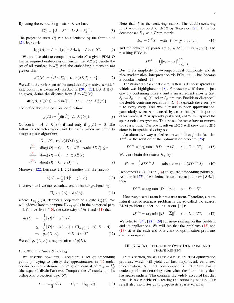
This problem is designed to model distance measurementsobtained by measuring the time of arrival of signals emittedfrom the sensors. Therefore, the large errors in ηi may benegative or positive, creating realistically diverse measurementerrors. Another difficult feature of this problem is that thesource has about 56% chance of lying outside of the convexhull of the known sensors. Table II reports the average local-ization error ‖xn−xn‖ over 1000 simulations, where xn is theestimated location and xn is the true location. It can be seenthat SSMDS yields the best performance in almost all casesexcept α = 0.9 in Case 2 and Case 3, for which HQMMDSworks better than FSMDS. We also plotted the results in Fig. 4for Case 2 for α varying from 0.1 to 1. It is obvious that theline by SSMDS is the lowest up to α = 0.9 and HQMMDSworks slightly better than SSMDS when α ≥ 0.9. This verifiesour theoretical result that SSMDS is particularly suitable toSSL problems. We also note that FSMDS, RMDS and TMDSall perform reasonably well.

TABLE II: Average error for Example 6.1 (N = 4) by the fivemethods over 1000 random simulations of each test instance.

MethodsCases α SSMDS FSMDS RMDS TMDS HQMMDS

Case 10.3 0.59 0.76 0.77 0.87 1.660.6 1.23 1.66 1.68 1.69 2.420.9 1.81 2.54 2.56 2.46 3.08

Case 20.3 0.79 1.04 1.06 1.08 1.930.6 0.36 0.40 0.39 0.54 1.190.9 0.83 1.06 1.09 1.21 0.75

Case 30.3 0.62 0.78 0.80 0.89 0.800.6 1.24 1.66 1.73 1.83 0.980.9 1.95 2.59 2.71 3.05 1.82

C. Real data: Motorola facility localization

The real data was obtained by the channel measurementexperiment conducted at the Motorola facility in Plantation,which is reported in [16]. The experiment environment is anoffice area which is partitioned by cubicle walls. 44 devicelocations are identified within a 14m × 13m area. Four of

10

Fig. 4: Average error (RMSE) vs α varying from 0.1 to 1 forCase 2 in Example 6.2 over 1000 simulations of test data.

the devices labelled as 3, 11, 35, 44 are chosen to be anchorsand remaining locations are unknown. In this experiment,each node can communicate with all other nodes. We use theoriginal time-of-arrival (TOA) to obtain the pairwise rangemeasurements: δij = c × T−TOAij , where c is the speedof light in terms of meters and T−TOAij is the measuredTOA between device i and j after removing the mean timedelay error (details see [16]). This implies that all of themeasurements have large errors (positive or negative). Inparticular, there are 37 negative pairwise distances in ∆ (Inour test, we replace them by |δij |). This data has been studiedin [15], where a few latest state-of-art methods based on Semi-Definite Programming (SDP) were tested. The reported resultsthere indicates that it would be challenging to achieve RMSEless than 1 meter for the unknown facilities.

We use this example to demonstrate two important strategiesthat are able to drive RMSE below 1m and that have notbeen explored in the two previous examples. One is usingthe weights Wij to distinguish importance of individual δij tothe objective. The other is enforcing tighter lower and upperbounds in (21).

(a) Sammon weighting scheme. It is a popular choice inscaling dissimilarity data proposed by Sammon [37], see also[2, P.255]. Each weight Wij is inversely proportional to δij .In our test, we used Wij = α/δij with α = 3 for δij 6= 0and 0 otherwise. Here α > 0 is balancing parameter, whichactually can be factorized into the penalty and smoothingparameter ρ and µ. A generalized choice is Wij = δqij withq ∈ < being properly chosen and is proposed in [38]. Wenote that the standard choice Wij = 1 when δij 6= 0 and0 otherwise simply indicates that for the point pair (i, j)a dissimilarity δij is available. The results are reported inTable III for both types of weights. It can be clearly seen thatSammon weights effectively drove RMSE below 1m for bothSSMDS and FSMDS. All other methods are not affected bythe different weighting choices. It is worth noting that RMDSand HQMMDS can also be adapted to include weights. But

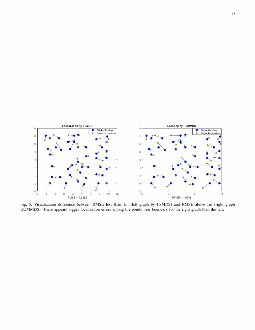
the implementations we obtained do not have such flexibility.The visualization of the obtained localization for the databy FSMDS and HQMMDS was plotted in Fig. 5. It is notsurprising to note that TMDS completely failed this databecause there are too many outliers and TMDS is mainlydesigned for situations with sparse outliers.

TABLE III: Effect of Sammon weights on RMSE for Motoroladata with α = 3 and ρ = 20, µ = 90 for SSMDS and FSMDS,and λ1 = 20, λ2 = 100 for HQMMDS.

MethodsWeights SSMDS FSMDS RMDS TMDS HQMMDSStandard 1.24 1.17 1.09 9.94 1.04Sammon 0.96 0.94 1.09 9.94 1.04

(b) Adding tighter lower and upper bounds. In theprevious tests, we simply set the lower bound Lij = 0 and theupper bounds Uij big numbers. If we were able to increase thelower bounds and decrease the upper bounds toward their truevalues dtrue

ij = ‖xi − xj‖, then we expect that the resultinglocalization will become more accurate. For example, let

`ij := βdtrueij and uij := (2− β)dtrue

ij .

As β varies from 0 to 1, the bounds in (21) with Lij = `2ijand Uij = u2

ij become tighter. In the extreme case, β = 1, thebounds are true and should result in the true location. This isdemonstrated in Fig. 6, where we considered three scenarioswith FSMDS: (i) only increase the lower bounds (FSMDS-lb); (ii) only decrease the upper bounds (FSMDS-ub); and(iii) increase the lower bounds and decrease the upper boundssimultaneously.

We note that all three scenarios result in improvement interms of RMSE accuracy and they all get better and betteras the bounds get tighter. However, there were limits forboth FSMDS-lb and FSMDS-ub. At the extreme β = 1 (thelower bounds or the upper bounds are true), the correspondingRMSE is between 0.4 and 0.5 and they cannot get smaller.In contrast, the best improvement occurred when the bothbounds are enforced simultaneously. At the extreme, FSMDS-lu recover the true positions of the facilities. We also like tonote that in practice, there would incur extra cost for obtainingtighter bounds. Fortunately there are many applications wheresuch tighter bounds (known as interval distance geometry) areavailable, see a recent survey [41]. It is also important to notethat while SSMDS and FSMDS have the capability of handlingthe lower and upper bounds without any extra cost, it is notknown how other methods such as RMDS and HQMMDS canhandle such constraints.

VII. CONCLUSION

cMDS has been a classical method for analyzing dissimi-larity data and it is widely known that it spreads errors amongall dissimilarities causing undesirable embeddings. This paperprovides a brand new interpretation of cMDS and casts itas a joint optimization problem with one variable residingin the almost positive semidefinite cone Kn+ and the otherin the subspace Sn2 . This new reformulation also reveals why

11

Fig. 6: Power of adding lower and upper bounds: as the boundsget tighter as β increases, FSMDS yields better localization.FSMDS-lb: adding lower bounds only; FSMDS-ub: addingupper bounds only; FSMDS-lu: adding both lower and upperbounds simultaneously.

cMDS tends to overly denoise even there is just one erroneousdissimilarity and naturally leads us to consider a subspaceMDS and its full-space variant FSMDS. We established theirconvergence results and compared them with several sate-of-the-art methods for outlier removal. Our numerical resultson synthetic and real data demonstrate their capability ofrecovering high-quality embedding. In particular, we are ableto handle the lower and upper bounds constraints, which couldcreate huge challenging for other methods. For some appli-cations such as the Motorola facility localization, enforcingquality lower and upper bounds is an effective (maybe theonly way) to improve localization accuracy. This importantcapability of ours is due to the Euclidean distance matrix(EDM) optimization we employed.

In terms of the objectives, ours is based on the cMDSand both RMDS and HQMMDS are based on the stressfunction in MDS. One advantage of cMDS objective is itscontinuous differentiability when put in EDM optimization,which subsequently simplifies our proof analysis. It will beour next research topic to see if the proposed framework canbe extended to the stress function, which would result in non-differentiability in its EDM reformulation.

ACKNOWLEDGEMENT

The authors would like to thank Fotios Mandanas forsharing his excellent code HQMMDS.

APPENDIX APROOF OF THEOREM 3.1

The proof is contained in the supporting file (Proof ofTheorem 3.1).

APPENDIX BPROOF OF THEOREM 5.1

Please refer to Sect. II and Sect. V for the definition ofthe functions g(D), h(D), gm(D,A) and F (D,Z), Fµ(D,Z),Fρ,µ(D,Z) and its majorization function Fmρ,µ(D,Z,Dk, Zk).We further let ϕ(Z) := ‖Z‖1 − ‖Z‖. We will need thefollowing inequalities.

h(−Dk+1)− h(−Dk) ≥ 〈ΠKn+(r)(−Dk), Dk −Dk+1〉 (36)

due to the convexity of h(·) and ΠKn+(r)(−Dk) ∈ ∂h(−Dk)

by (11).Since Dk+1 = arg minF (D,Zk) + ρgm(D,Dk), the opti-

mality condition holds at Dk+1:

〈Ωk+1, D −Dk+1〉 ≥ 0, ∀ D ∈ B, (37)

where Ωk+1 := ∇DF (Dk+1, Zk)+ρ(Dk+1+ΠKn+(r)(−Dk)).

Since Zk+1 = arg minF (Dk+1, Z) + µ(‖Z‖1 − 〈T k, Z〉),the optimality condition holds at Zk+1: There exists Γk+1 ∈∂‖Zk+1‖1 such that

∇ZF (Dk+1, Zk+1) + µ(Γk+1 − T k) = 0. (38)

Define the quantity

τk := 〈∇ZF (Dk+1, Zk+1), Zk−Zk+1〉+µ(ϕ(Zk)−ϕ(Zk+1).

We claimLemma B.1: τk ≥ 0.

Proof: It is known that for the one-dimensional absolutevalue function |x|, its subdifferential is defined as

∂|x| =

1 if x > 0[−1, 1] if x = 0−1 if x < 0.

One consequence is that ξx = |x| and and |ξ| ≤ 1 for anyξ ∈ ∂|x|. Applying this fact to Γk+1 ∈ ∂‖Zk+1‖1 yields

〈Γk+1, Zk+1〉 = ‖Zk+1‖1, 〈Γk+1, Z〉 ≤ ‖Z‖1,∀ Z. (39)

Now computing the inner product with (Zk −Zk+1) on bothsides of (38) leads to

〈∇ZF (Dk+1, Zk+1), Zk − Zk+1〉= µ〈Γk+1 − T k, Zk+1 − Zk〉= µ〈Γk+1, Zk+1〉 − µ〈Γk+1, Zk〉 − µ〈T k, Zk+1 − Zk〉

(39)= µ‖Zk+1‖1 − µ〈Γk+1, Zk〉 − µ〈T k, Zk+1 − Zk〉.

Substituting the above into τk and simplifying to get

τk = µ(‖Zk‖1 − 〈Zk,Γk+1〉︸ ︷︷ ︸≥0 due to (39)

)+µ(‖Zk+1‖ − ‖Zk‖ − 〈T k, Zk+1 − Zk〉︸ ︷︷ ︸≥0 due to the convexity of ‖Z‖

)

This completes the proof.

12

The following two identities can be verified directly.

‖Dk+1‖2 − ‖Dk‖2

= 2〈Dk+1 −Dk, Dk+1〉 − ‖Dk+1 −Dk‖2. (40)

∇DF (Dk+1, Zk+1)−∇DF (Dk+1, Zk)

= (W W ) (Zk+1 − Zk). (41)

Proof: (Thm. 5.1) (i) Since B is bounded, Dk is sobecause Dk ∈ B. Now suppose Zk is not bounded. Theremust exists a subsequence indexed by ki such that |Zki`j | →∞ for some fixed (`, j). According to the update rule (33),we must have W`j > 0 (otherwise Zk`,j = 0 for all k). Thenonincreasing property of Fρ,µ(Dk, Zk) yields

Fρ,µ(D0, Z0) ≥ Fρ,µ(Dki , Zki) ≥ F (Dki , Zki)

≥ 1

2W 2`j

(∆`j −Dki

`j − Zki`j

)2

→∞

due to the boundedness of Dk. This contradiction estab-lishes the boundedness of Zk.

(ii) This part of the proof involves a considerable amountof calculation, but most of them are simple. The first fact weused (the second equality below) is the exact Taylor expansionof F (D,Z) at (Dk+1, Zk+1) since F (D,Z) is quadratic.

Fρ,µ(Dk, Zk)− Fρ,µ(Dk+1, Zk+1)

= F (Dk, Zk)− F (Dk+1, Zk+1)

+ ρ(g(Dk)− g(Dk+1) + µ(ϕ(Zk)− ϕ(Zk+1))

= 〈∇DF (Dk+1, Zk+1)︸ ︷︷ ︸apply (41)

, Dk −Dk+1〉

+ 〈∇ZF (Dk+1, Zk+1), Zk − Zk+1〉

+1

2〈W (Dk −Dk+1), W (Dk −Dk+1)〉︸ ︷︷ ︸

≥0

+1

2〈W (Zk − Zk+1), W (Zk − Zk+1)〉

+ 〈W (Zk − Zk+1), W (Dk −Dk+1)〉+

ρ

2

(‖Dk‖2 − ‖Dk+1‖2︸ ︷︷ ︸

apply (40)

)+ ρ(h(−Dk+1)− h(−Dk)︸ ︷︷ ︸

apply (36)

)+ µ(ϕ(Zk)− ϕ(Zk+1))

≥ 〈Ωk+1, Dk −Dk+1〉︸ ︷︷ ︸

≥0 by (37)

+ρ

2‖Dk −Dk+1‖2

+ 〈∇Zf(Dk+1, Zk+1), Zk − Zk+1〉

+1

2〈W (Zk − Zk+1), W (Zk − Zk+1)〉

+ µ(ϕ(Zk)− ϕ(Zk+1))

≥ ρ

2‖Dk −Dk+1‖2 + τk

+1

2〈W (Zk − Zk+1), W (Zk − Zk+1)〉.

Lemma B.1 (τk ≥ 0) establishes the first claim in (ii).Since Fρ,µ(Dk, Zk) is bounded below by 0, we must have

limFρ,µ(Dk, Zk) − Fρ,µ(Dk+1, Zk+1) → 0, which forces(Dk+1 − Dk) → 0 and Zk+1

`j − Zk`j → 0 when W`j > 0.

However, Zk`j = 0 for all k when W`j = 0. Hence, we alsohave (Zk − Zk+1)→ 0.

(iii) Suppose (D∗, Z∗) is the limit of a subsequenceDk, Zkk∈K . It follows from (ii) that Dk+1 → D∗ andZk+1 → Z∗ for k ∈ K. Since the subgradient sequenceΓk+1k∈K and Zk+1k∈K are bounded, without loss ofgenerality we may assume Γk+1 → Γ∗ and T k → T ∗.

By the upper semicontinuity of the subdifferentials of con-vex functions, we have

Γ∗ ∈ ∂‖Z∗‖1 and T ∗ ∈ ∂‖Z∗‖.

Taking the limits on both sides of (38) for k ∈ K to obtain

∇ZF (D∗, Z∗) + µ(Γ∗ − T ∗) = 0.

And taking the limits on both sides of (37) for k ∈ K toobtain

〈∇DF (D∗, Z∗) + ρ(D∗ + ΠKn+(r)(−D∗)), D −D∗〉 ≥ 0

for all D ∈ B. These two conditions are the optimalityconditions in (35). This completes our proof.

APPENDIX CPROOF OF THEOREM 5.2

Proof: The proof technique is taken from [30]. It followsfrom (38) that

∇ZF (Dk, Zk) + µ(Γk − T k−1) = 0,

where Γk ∈ ∂‖Zk‖1 and T k−1 ∈ ∂‖Zk−1‖. Therefore,‖T k−1‖ ≤ 1 and ‖Γk‖ ≥

√‖Zk‖0, which imply

‖∇ZF (Dk, Zk)‖ = µ‖Γk − T k−1‖

≥ µ(‖Γk‖ − ‖T k−1‖

)≥ µ

(√‖Zk‖0 − 1

).

On the other hand, using

∇ZF (Dk, Zk) = W W (Dk + Zk −∆),

we obtain

‖∇ZF (Dk, Zk)‖ ≤ wmax‖W (Dk + Zk −∆)‖,

where wmax := maxWij. We further note that

1

2‖W (Dk + Zk −∆)‖2 ≤ Fρ,µ(Dk, Zk) ≤ Fρ,µ(D0, 0)

Putting the two bounds on ‖W (Dk + Zk − ∆)‖ togetheryields √

‖Zk‖0 − 1 ≤wmax

√2Fρ,µ(D0, 0)

µ,

which means that µs > 0 can be selected as in the theorem.We note that Fρ,µ(D0, 0) does not depend on µ.

13

REFERENCES

[1] T.F. Cox and M.A.A. Cox, Multidimensional Scaling, 2nd Ed, Chapmanand Hall/CRC, 2001.

[2] I. Borg and P.J.F. Groenen, Modern Multidimensional Scaling: Theoryand Applications, 2nd Ed., Springer Series in Statistics, Springer, 2005.

[3] I.J. Schoenberg, “Remarks to Maurice Frechet’s article Sur la definitionaxiomatque d’une classe d’espaces vectoriels distancies applicbles vecto-riellement sur l’espace de Hilbet”, Ann. Math., 36, pp. 724-732, 1935.

[4] G. Young and A.S. Householder, “Discussion of a set of points in termsof their mutual distances”, Psychometrika, 3, pp. 19-22, 1938.

[5] J.C. Gower, “Some distance properties of latent root and vector methodsused in multivariate analysis”, Biometrika, 53, pp. 325–338, 1966.

[6] J.B. Tenenbaum, V. de Silva and J.C. Langford, “A global geometricframework for nonlinear dimensionality reduction”, Science, 290, pp.2319-2323, 2000.

[7] R. Sibson “Studies in the robustness of multidimensional scaling: per-turbational analysis of classical scaling”, J. Royal Statistical Society, B,41(2), 217–219, 1979.

[8] L. Cayton and S. Dasgupta “Robust Euclidean embedding”, Proceedingsof the 23rd International Conference on Machine Learning, Pittsburgh,PA 2006, pp. 169–176.

[9] P.A. Forero and G.B. Giannakis, “Sparsity-exploiting robust multidimen-sional scaling”, IEEE Trans. Signal Process., 60(8), pp. 4118-4134, 2012.

[10] J.B. Kruskal. “Nonmetric multidimensional scaling: a numericalmethod”, Psychometrika, 29, pp. 115-129, 1964.

[11] F.D. Mandanas and C.L. Kotropoulos, “Robust multidimensional scalingusing a maximum correntropy criterion”, IEEE Trans. Signal Process.,65(4), pp. 919-932, 2017.

[12] F.D. Mandanas and C.L. Kotropoulos, “M-estimators for robust multi-dimensional scaling employing `21-norm regularization”, Pattern Recog-nition, 73, 235-246, 2018.

[13] H. Chen, G. Wang, Z. Wang, H. C. So, and H. V. Poor, “Non-Line-of-Sight node localization based on semi-definite programming in wirelesssensor networks”, IEEE Trans. Wireless Commun., 11, 108-116, 2012.

[14] R.M. Vaghefi, J. Schloemann, and R.M. Buehrer, “NLOS mitigationin TOA-based localization using semidefinite programming”, PositioningNavigation and Communication (WPNC), 2013, pp. 1-6.

[15] C. Ding and H.-D. Qi, “Convex Euclidean distance embedding forcollaborative position localization with NLOS mitigation”, Comput OptimAppl., 66, 187-218, 2017.

[16] N. Patwari, A. O. Hero, M. Perkins, N. S. Correal, and R. J. O’Dea,“Relative location estimation in wireless sensor networks”, IEEE Tran.Signal Processing, 51, 21372148, 2003.

[17] G. Wang, A. M-C. So and Y. Li, “Robust convex approximation methodsfor TDOA-based localization under NLOS conditions”, IEEE Trans.Signal Process., 64(13), 3281-3296, 2016.

[18] A. Beck, P. Stoica, and J. Li, “Exact and approximate solutions ofsource localization problems”, IEEE Tran. Signal. Process., 56, 1770–1778, 2008.

[19] H.-D. Qi, N.H. Xiu, and X.M. Yuan, “A Lagrangian dual approach tothe single source localization problem”, IEEE Tran. Signal Process., 61,3815–3826, 2013.

[20] H.-D. Qi and X.M. Yuan, “Computing the Nearest Euclidean DistanceMatrix with Low Embedding Dimensions”, Math. Prog., 147, pp. 351-389, 2014.

[21] I. Dokmanic, R. Parhizkar, J. Ranieri and M. Vetterli, “Euclideandistance matrices: Essential theory, algorithms, and applications”, IEEESignal Process. Mag., 32(6), pp. 12-30, 2015.

[22] S. Zhou, N.H. Xiu and H.-D. Qi, “A fast matrix majorization-projectionmethod for penalized stress minimization with box constraints”, IEEETrans. Signal Process., 66, pp. 4331-4346, 2018.

[23] R. Tibshirani, “Regression shrinkage and selection via the Lasso”, J.Roy. Stat. Soc. B, 58, 267-288, 1996.

[24] N. Gaffke and R. Mathar, “A cyclic projection algorithm via duality”,Metrika, 36, pp. 29-54, 1989.

[25] W.S. Torgerson, “Multidimensional scaling: I. Theory and method”,Psychometrika, 17(4), pp. 401-419, 1952.

[26] K.V. Mardia, “Some properties of classical mulitidimensional scaling”,Comm. Statist. A – Theory Methods, A7:1233-1243, 1978.

[27] R. Mathar, “The best Euclidean fit to a given distance matrix inprescribed dimensions”, Linear Alge. Appli. 67, 1-6, 1985.

[28] W. Glunt, T.L. Hayden, S. Hong and J. Wells, “An alternating projectionalgorithm for computing the nearest Euclidean distance matrix”, SIAM J.Matrix Anal. Appl., 11, pp. 589-600, 1990.

[29] H.-D. Qi, “A semismooth Newton method for the nearest Euclideandistance matrix problem”, SIAM J. Matrix Anal. Appl., 34, pp. 67-93,2013.

[30] P. Yin, Y. Lou, Q. He, and J. Xin, “Minimization of `1−2 for compressedsensing”, SIAM J. Sci. Comput., 37, A536-A563, 2015.

[31] J. de Leeuw and P. Mair, “Multidimensional scaling using majorization:Smacof in R”, J. Stat. Software, 31, pp. 1-30, 2009.

[32] Y. Sun, P. Babu and D.P. Palomar, “Majorization-minimization algo-rithms in signal processing, communications, and machine learning”,IEEE Trans. Signal Process., 65(3), pp. 794-816, 2017.

[33] R.A. Horn and C.R. Johnson, “Topics in Matrix Analysis”, Vol. 2,Cambridge University Press, 1991.

[34] E.C. Chu, H. Zhou and K. Lange, “Distance majorization and itsapplications”, Math. Program., 146, 409-436, 2014.

[35] K.S. Arun, T.S. Huang, S.D. Blosten, “Least-squares fitting of two 3-Dpoint sets”, IEEE Trans. Pattern Anal. Machine Intell., 9 (1987), 698-700.

[36] R. Sanyal, M. Jaiswal and K.N. Chaudhury, “On a registration-basedapproach to sensor network localization”, IEEE Trans. Signal Process.,65 (2017), 5357-5367.

[37] J.W. Sammon, “A non-linear mapping for data structure analysis”, IEEETrans. on Computers, 18 (1969), 401-409.

[38] A. Buja and D.F. Swayne, “Visualization methodology for multidimen-sional scaling”, J. Classification, 19 (2002), 7-44.

[39] L. Blouvshtein and D. Cohen-Or, “Outlier detection for robust multi-dimensional scaling”, IEEE Trans. Pattern Recog. Machine Intell. 2018.

[40] C.A. Micchelli, “Interpolation of scattered data: distance matrices andconditionally positive definite functions”, Constr. Approx., 2, 11-22, 1986.

[41] D.S. Goncalves, A. Mucherino, C. Lavor, and L. Liberti, “Recentadvances on the interval distance geometry problem”, J. Global Optim.,69 (2017), 525-545.

14

PROOF OF THEOREM 3.1

We need the following result, which is a restatement of aresult in [40].

Lemma C.1: [40, Cor. 2.1(a)] Let Kn+ be the conditionallypositive semidefinite cone, Dn be the EDM cone and Sn2 bethe subspace defined in (18). Then it holds

Kn− = Dn + Sn2 , (42)

where Kn− := −Kn+. Moreover, the decomposition in (42) isunique in the sense that for any given matrix A ∈ Kn−, thereexist unique D ∈ Dn and Z ∈ Sn2 such that A = D+Z with

D = A− Z and Z := a1T + 1aT , a :=1

2diag(A).

Proof: (Thm. 3.1) The proof is in three parts: (i) We provethe optimization problem has a unique solution (D, Z); (ii) weprove D = Dmds; and (iii) we prove Z takes the form givenin the theorem.

(i) Lemma C.1 implies that the joint optimization problem(19) is equivalent to

min ‖∆−A‖2, s.t. A ∈ Kn−.

This is the projection problem onto the convex cone Kn−. Itsunique optimal solution is A := ΠKn

−(∆), and the correspond-

ing unique (D, Z) are

D = A− Z, Z = a1T + 1aT , a :=1

2diag(A).

(ii) It follows from (6) that

A = ΠKn−

(∆) = −ΠKn+

(−∆) = ∆−ΠSn+

(J∆J). (43)

We note (by direct verification) that

J = Q

[In−1 0

0 0

]Q, with Q := I − 1

n+√nvvT (44)

and vT := (1, . . . , 1,√n+1) ∈ <n. Here, In−1 is the identity

matrix in Sn−1 and Q is known as a Householder matrixsatisfying Q2 = I . Therefore,

J∆J = Q

[In−1 0

0 0

]Q∆Q

[In−1 0

0 0

]Q

= Q

[∆1 00 0

]Q,

where ∆1 is the leading (n−1)× (n−1) block of the matrixQ∆Q. Since Q is orthogonal, we have

ΠSn+

(J∆J) = Q

[ΠSn−1

+(∆1) 0

0 0

]Q (45)

and

QΠSn+

(J∆J)Q =

[ΠSn−1

+(∆1) 0

0 0

]. (46)

Furthermore,

JΠSn+

(J∆J)J

(44)= Q

[In−1 0

0 0

]QΠSn

+(J∆J)Q

[In−1 0

0 0

]Q

(46)= Q

[In−1 0

0 0

] [ΠSn−1

+(∆1) 0

0 0

] [In−1 0

0 0

]Q

= Q

[ΠSn−1

+(∆1) 0

0 0

]Q

(45)= ΠSn

+(J∆J). (47)

Since J1 = 0, we have JZJ = 0. Putting those facts together,we have

JDJ = J(A− Z)J = JAJ(43)= J∆J − JΠSn

+(J∆J)J

(47)= J∆J −ΠSn

+(J∆J)

= −ΠSn+

(−J∆J),

where the last equation used the fact

X = ΠSn+

(X)−ΠSn+

(−X), ∀ X ∈ Sn.

Consequently, we have

−1

2JDJ =

1

2ΠSn

+(−J∆J)

(13)= B+.

Since D ∈ Dn, it follows from (16) that D can be generatedby the decomposition of B+ in (14): Dij = ‖yi−yj‖2. Hence,we must have D = Dmds.

(iii) Since we have established D = Dmds, the optimal Zmust be the optimal solution of the following problem:

minZ∈Sn

2

f(Z) =1

2‖(Dmds + Z)−∆‖2F

=1

2‖(Dmds + z1T + 1zT )−∆‖2F ,

with z ∈ <n. Recall C := ∆−Dmds, we have

f(z) =1

2‖C‖2F − 2〈C1, z〉+ n‖z‖2 + (1T z)2.

Since f(z) is convex, its gradient must vanish at its optimalsolution z:

0 = ∇f(z) = −2C1 + 2nz + 2(1T z)1.

Computing the inner product with 1 on both sides of the aboveequation yields

1T z =1

2n1TC1,

which in turn gives rise to

z = − 1

nC1− 1

2n21TC1 = c− 1

2c1.

The optimal solution Z = z1T +1zT , which is what we statedin the theorem.

15

Fig. 5: Visualization difference between RMSE less than 1m (left graph by FSMDS) and RMSE above 1m (right graphHQMMDS): There appears bigger localization errors among the points near boundary for the right graph than the left.