1-1 1 Text from the Manuscript for Classical Thermodynamics 1/e Subrata Bhattacharjee THIS MATERIAL MAY NOT BE DUPLICATED IN ANY FORM AND IS PROTECTED UNDER ALL COPYRIGHT LAWS AS THEY CURRENTLY EXIST. No part of this material may be reproduced, in any form or by any means, without permission in writing from the Publisher. 2004 Pearson Education, Inc. Prentice Hall Upper Saddle River, NJ 07458 This publication is protected by United States copyright laws, and is designed exclusively to assist instructors in teaching their courses. It should not be made available to students, or to anyone except the authorized instructor to whom it was provided by the publisher, and should not be sold by anyone under any circumstances. Publication or widespread dissemination (i.e. dissemination of more than extremely limited extracts within the classroom setting) of any part of this material (such as by posting on the World Wide Web) is not authorized, and any such dissemination will violate the United States copyright laws. In consideration of the authors, your colleagues who do not want their students to have access to these materials, and the publisher, please respect these restrictions
Transcript
1-1
1
Text from the Manuscript for
Classical Thermodynamics 1/e
Subrata Bhattacharjee
THIS MATERIAL MAY NOT BE DUPLICATED IN ANY FORM AND IS PROTECTED UNDER ALL
COPYRIGHT LAWS AS THEY CURRENTLY EXIST.
No part of this material may be reproduced, in any form or by any means, without
permission in writing from the Publisher.
2004 Pearson Education, Inc. Prentice Hall Upper Saddle River, NJ 07458
This publication is protected by United States copyright laws, and is designed exclusively to assist instructors in teaching their courses. It should not be made available to students, or to anyone except the authorized instructor to whom it was provided by the publisher, and should not be sold by anyone under any circumstances. Publication or widespread dissemination (i.e. dissemination of more than extremely limited extracts within the classroom setting) of any part of this material (such as by posting on the World Wide Web) is not authorized, and any such dissemination will violate the United States copyright laws. In consideration of the authors, your colleagues who do not want their students to have access to these materials, and the publisher, please respect these restrictions
1-2
BASIC CONCEPTS – SYSTEMS, INTERACTIONS, STATES AND PROPERTIES
Thermodynamics is a word derived from the Greek words thermo (meaning energy or
temperature) and dunamikos (meaning movement). It began its origin as the study of
converting heat to work, that is, energy into movements. Today, scientists use the
principles of thermodynamics to study the physical and chemical properties of matter.
Engineers, on the other hand, apply thermodynamic principles to understand how the
state of a practical system responds to interactions – transfer of mass, heat, and work -
between the system and its surroundings. This understanding allows for more efficient
designs of thermal systems that include steam power plants, gas turbines, rocket engines,
internal combustion engines, a refrigeration plants, air conditioning units, to name a few.
This chapter introduces the basic concepts of thermodynamics, in particular – the
definition of a system, its surroundings, mass, heat and work interactions, the concept of
equilibrium, as well as a description of a system through its states and properties.
Throughout this book we will adhere to Systeme International or SI units in
developing theories and understanding basic concepts, while using mixed units - a
combination of SI and English systems - for problem solving.
The courseware TEST, accessible from www.thermofluids.net, will be used
throughout this book for several purposes. The online tutorial is the best resource to get
updated information on, especially on the frequently used modules: (i) Animations that
are used to supplement discussions throughout this textbook; (ii) Web-based
thermodynamic calculators called daemons that are used to develop a quantitative
understanding of thermodynamic properties, step-by-step verification of manual
solutions, and occasional what-if studies for additional insight; (iii) Example and Problem
modules that present multimedia-enriched examples and end-of-chapter problems; (iv)
Rich internet applications or RIAs to simulate complex systems such as a reacting
system, a gas turbine or an internal combustion engine.
Subrata Bhattacharjee ....................................................................................... 1-1 BASIC CONCEPTS – SYSTEMS, INTERACTIONS, STATES AND PROPERTIES 1-2
1.1 Thermodynamic Systems ................................................................................. 1-5 1.1.1 TEST and Animations ...................................................... 1-7
1.1.2 Examples of Thermodynamic Systems ............................ 1-7 1.2 Interactions between System and Surroundings ............................................ 1-10
1.2.1 Mass Interaction ............................................................. 1-11 1.2.2 TEST and the Daemons .................................................. 1-13
1.2.3 Energy , Work , and Heat ............................................... 1-14
1.2.5 Work and Power (W , W ) .............................................. 1-21 1.2.6 Work Transfer Mechanisms ........................................... 1-22
A. Mechanical Work ( , M MW W ) .................................................................. 1-22
B. Shaft Work ( sh sh, W W ) ............................................................................. 1-25
C. Electrical Work ( el el, W W ) ....................................................................... 1-25
D. Boundary Work ( , B BW W ) ....................................................................... 1-26
E. Flow Work ( FW ) ..................................................................................... 1-30
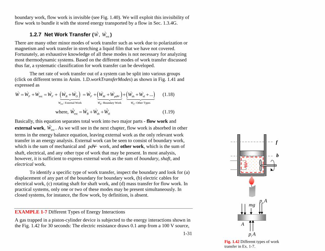
1.2.7 Net Work Transfer ( ext, W W ) ......................................... 1-31
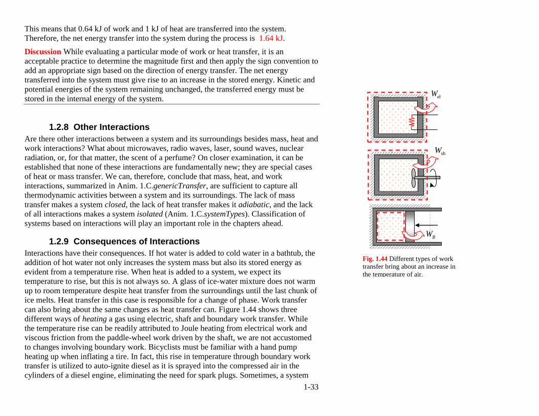
1.2.8 Other Interactions ........................................................... 1-33 1.2.9 Consequences of Interactions ......................................... 1-33
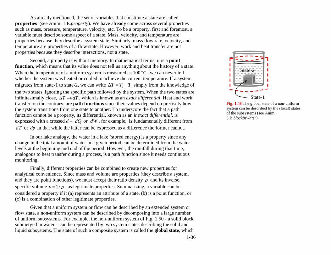
1.3 States and Properties ...................................................................................... 1-34
1.3.1 Macroscopic vs. Microscopic Thermodynamics ............ 1-37
1.3.2 An Image Analogy ......................................................... 1-38 1.3.3 TEST and the State Daemons ......................................... 1-39
1.3.4 Properties of State .......................................................... 1-43
A. Properties Related to System Size ( , , , , , , V A m n m V n ) .................... 1-44
B. Density and Specific Volume ( , v ) ...................................................... 1-46
C. Velocity and Elevation ( , V z )................................................................. 1-48
D. Pressure ( p ) ............................................................................................ 1-49
E. Temperature (T ) ...................................................................................... 1-54
F. Stored Energy ( E , KE , PE , U , e , ke , pe , u , E ) .............................. 1-57
1-4
G. Flow Energy and Enthalpy ( , , , j J h H ) ................................................ 1-62
H. Entropy ( S , s ) ........................................................................................ 1-65
I. Exergy ( , ) ............................................................................................. 1-69
Index .......................................................................................................................... 1-72
1-5
1.1 Thermodynamic Systems
We are all familiar with the concept of a free body diagram from our study of mechanics.
To analyze the force balance on a body, or a portion of it, we isolate the region of interest
with real or fictitious boundaries and call it a free body (see Anims1. 1.A.weight through
1.A.vacuumPressure) and identify all the external forces exerted on the surface and
interior of the free body. For instance, take a look at Fig. 1.1. To determine the net
reaction force R necessary to hold the book stationary, we isolate the book and draw all
the vertical forces acting on it. Due to the fact that the ambient air applies uniform
pressure all over the exposed surfaces, there is no net contribution from the atmosphere.
We will discuss pressure in a more thorough manner in sections to come. At this point it
is sufficient to understand pressure as the intensity of perpendicular compressive force
exerted by a fluid on a surface. In SI units pressure is measured in kN/m2 or kPa and in
English units it is measured in psi. The reaction force R in Fig. 1.1, therefore, must be
equal to the weight of the book. Applying the same concept, we can obtain the pressure
inside the piston-cylinder device of Fig. 1.2 by drawing all the vertical forces acting on
the piston after isolating it through a free body diagram. The steps involved in such an
analysis are illustrated in Anim. 1.A.pressure and in Ex. 1-1.
Just as a free body diagram helps us analyze the force balance on a body, a
thermodynamic system helps us analyze the interactions between a system and its
surroundings.
In thermodynamics, a system is broadly defined as any entity of interest within a
well-defined boundary.
A thermodynamic system does not have to be a fixed mass as in mechanics, but can be a
practical device such as a pump or a turbine with all its possible interactions with
whatever lies outside its boundary. Even a complete vacuum can form a perfectly
legitimate system. The boundary of a system is carefully drawn by the analyst with the
objective of separating what is of interest from the rest of the world, known as its
surroundings. Together, the system and its surroundings form the thermodynamic
universe. For instance, if hot coffee within the black boundary in Fig. 1.3 constitutes the
system, then everything else – the mug, the desk, and the rest of the world for that
matter– make up the surroundings.
A boundary can be real or imaginary, rigid or non-rigid, stationary or mobile, and
internal or external with respect to the wall. The physical wall of a system, such as the
casing of a pump or the mug holding the coffee in Fig. 1.3, is often considered a non-
1 Sec. 1.1.1 walks you through VT animations.
THERMO mg
mgR
Fig. 1.1 Free body diagram of a textbook (see Anim.
1.A.weight).
THERMO
ip
Apo
mg
ApmgAp oi
Fig. 1.2 Force balance on a piston (see Anim.
1.A.pressure).
Internal boundary
External boundary
Fig. 1.3 Each boundary can be used in analyzing
the system – the coffee in the mug. In most
analyses, we will use the external boundary (see
Anim. 1.B.systemBoundary).
1-6
participant in the interactions between the system and its surroundings. As a result, the
boundary can be placed internally (black) or externally (red) without affecting the
solution (see Anim. 1.B.systemBoundary). The term internal system is sometimes used
to identify the system bordered within the internal boundary. In this book, the external
red boundary passing through the atmospheric air as in Fig. 1.2 will be our default choice
for system boundary unless an analysis requires consideration of the internal system.
EXAMPLE 1-1 Free body diagram
Determine (a) the pressure inside the cylinder as shown in the accompanying figure in
kN/m2
from the following data: Area of the piston is 25 cm2, mass of the hanging weight
is 10 kg, atmospheric pressure is 100 kN/m2, and acceleration due to gravity is 9.81 m/s
2.
What-if scenario: (b) what is the maximum possible mass that could be supported by this
configuration?
SOLUTION Draw a free body diagram of the piston. A horizontal force balance
produces the desired answer.
Assumptions Neglect friction, if any, between the piston and the cylinder.
Analysis The free body diagram of the piston is shown in Fig. 1.4. A horizontal force
balance yields
2
piston 0 piston 2 2
kN m kN m kg kN
1000 N/kN m s Ni
mgp A p A
0 4piston
2
10 9.81 100
1000 N/kN 1000 N/kN 25
kN60.
1076
mi
mgp p
A
What-if Scenario As m is increased to a new value, the piston will move to the right
and then come to a new equilibrium position. With 0p and pistonA remaining constant, ip
will decrease according to the horizontal force balance presented above. Since pressure is
always compressive by nature, the minimum value of ip is zero. Therefore, the
maximum mass that can supported is given as
ip
0max
0
piston
4
0 piston
max
1000 N/kN
100 25 10N N 100 25.48 0 1000
kN kN 9. 1g
8k
m gp
A
p Am
g
Did you know?
A 102 kg (225 lb) person weighs about 1 kN.
In thermodynamic applications, N turns out to be too small
for practical use. For instance, atmospheric pressure is
around 100 kPa or 100,000 N/m2. To avoid use of large
mg
Ap0 Api
Fig. 1.4 Schematic of an arrangement
creating a sub-atmospheric pressure in
Ex. 1-1 (see Anim.
1.A.vacuumPressure).
ip 0p
1-7
Discussion Notice the use of SI units in this problem. The unit of force used in
thermodynamics is kN as opposed to N in mechanics. The familiar expression for weight,
mg , therefore, must be divided by a unit conversion factor of 1000 N/kN to express the
force in kN. Browse Anim.1.A.vacuumPressure to gain more insight on the application
of free body diagram.
1.1.1 TEST and Animations
In this textbook, we will make frequent references to different modules of TEST – The
Expert System for Thermodynamics, accessible online from www.thermofluids.net or
installable in your computer from a CD. To set your browser to run TEST, read the
Getting Started section of the Tutorial linked from the TEST task bar.
Animations in TEST are organized following the structure of this book. They are
referenced by a standard format – a short title for the animation is preceded by the section
number and chapter number. For instance, Anim. 1.B.combustion can be accessed by
launching TEST, and then clicking the Animation link from the task bar, selecting
Chapter 1, Section B, and then combustion from the drop-down menu located in the
control panel of the animation slide. Many animations have active buttons, providing
interactive features. In Anim. 1.B.combustion, you can toggle between complete and
incomplete reactions by clicking the corresponding buttons. The RIAs (rich internet
application) have the same look and feel as animations, but take the concept further
where a complete thermal system such as a gas turbine or a combustion chamber can be
simulated.
1.1.2 Examples of Thermodynamic Systems
The generality of the definition of a thermodynamic system - any entity inside a well
defined boundary - makes the scope of thermodynamic analysis mind-boggling. Through
thermofluids.net
1-8
Fig. 1.5(a) See Anim.1.C.carEngine. Fig. 1.5(b) See Anim.1.C.closedMixing. Fig. 1.5(c) See Anim.1.C.compression.
Fig. 1.5(d) See Anim.1.C.charging. Fig. 1.5(e) See Anim.1.C.refrigerator. Fig. 1.5(f) See Anim.1.C.turbine.
1-9
suitable placement of a boundary, systems can be identified in applications ranging from
power plants, internal combustion engines, rockets, and jet engines to household
appliances such as air-conditioners, gas ranges, pressure cookers, refrigerators, water
heaters, propane tanks and even a hair dryer. Some samples of the thermodynamic
systems we are going to analyze in the coming chapters are illustrated by animations in
section 1.B (System Tour). This diverse range of systems, some of which are sketched in
Fig. 1.5, appears to have very little in common. Yet, upon close examination, they reveal
remarkably similar pattern in terms of how they interact with their surroundings. Let us
consider a few specific examples and explore these interactions qualitatively. We will use
the terms energy, heat, and work, which will be thoroughly introduced in a latter section,
loosely in the following discussion.
When we open the hood of a car, most of us are amazed by the complexity of the
modern automobile engine. However, if we familiarize ourselves with how an engine
works, the simplified system diagram shown in Fig. 1.5(a) ( Anim. 1.C.carEngine) can be
intuitively understood. While the transfer of mass (in the form of air, fuel, and exhaust
gases) and work (through the crank shaft) are obvious, to feel the heat radiating from the
hot engine we have to look under the hood.
Two rigid tanks containing two different gases are connected by a valve in Fig.
1.5(b) (Anim 1.C.closedMixing). As the valve is opened, the two gases flow and diffuse
into each other, eventually forming a uniform mixture. In analyzing this mixing process,
the complexity associated with the transfer of mass between the two tanks can be
completely avoided if the boundary is drawn to encompass both tanks within as shown in
the figure. If the system is insulated, there can be no mass, heat, or work transfer during
the mixing process.
The piston-cylinder device of Fig. 1.5(c) (Anim. 1.C.compression) can be found
at the heart of internal combustion engines and in reciprocating pumps and compressors.
If the gas being compressed is chosen as the system, there is no mass transfer.
Furthermore, if the compression takes place rapidly, there is little time for any significant
transfer of heat. The transfer of work between the system and the surroundings boils
down to analyzing the displacement of the piston (boundary) due to internal and external
forces present.
On the other hand, consider the completely evacuated rigid tank of Fig. 1.5(d)
(Anim. 1.C.charging). As the valve is opened, outside air rushes in to fill up the tank and
equalize the pressure between the inside and outside. What is not trivial about this
process is that air that enters becomes hot – hotter than the boiling temperature of water
at atmospheric pressure. There is mass and work transfer as air is pushed in by the
System
Surroundings
Mass
Heat
Work
Fig. 1.6 Mass and energy interactions between a
system and its surroundings are independent of
whether internal (black) or external (red) boundary is
chosen (see Anim. 1.B.systemBoundary).
1-10
outside atmosphere, but heat transfer may be negligible if the tank is insulated or the
process takes place very rapidly.
Let us now consider the household refrigerator shown in Fig. 1.5(e) (Anim.
1.C.refrigerator). Energy is transferred into the system through the electric cord to run
the compressor, which constitutes work transfer in the form of electricity. Although a
refrigerator is insulated, some amount of heat leaks in through the seals and walls into the
cold space maintained by the refrigerator. To keep the refrigerator temperature from
going up, heat must be „pumped‟ out of the system. Indeed, if we can locate the
condenser, a coil of narrow finned tube placed behind or under a unit, we will find it to be
warm. Heat, therefore, must be rejected into the cooler atmosphere, thereby removing
energy from the refrigerator. Heat and electrical work transfer are the only interactions in
this case.
Finally, the steam turbine of Fig. 1.5(f) (or Anim. 1.C.turbine) extracts part of the
energy transported by steam into the turbine and delivers it as external work to the shaft.
Although the boundary of the extended system may enclose all the physical hardware –
casing, blades, nozzles, shaft, etc. - the actual analysis only involves mass, heat and work
transfer across the boundary and the presence of the hardware can be ignored without any
significant effect on the solution.
In this discussion our focus has been on the interactions between the system and
the surroundings at the boundary. In fact, there is no need to complicate a system diagram
with the complexities of its internal workings. An abstract or generic system sketched in
Fig. 1.6 (or Anim. 1.C.genericTransfer) can represent each system discussed in this
section quite adequately since it incorporates all possible interactions between a system
and its surroundings, which are discussed next. As mentioned before, the choice of
external or internal boundary cannot change the nature or the degree of these interactions.
1.2 Interactions between System and Surroundings
A careful examination of all interactions discussed in the earlier section will reveal that
interactions between a system and its surroundings fall into one of the three fundamental
categories – transfer of mass, heat or work (see Fig. 1.6). A thorough understanding of
these interactions is necessary for any thermodynamic analysis, whose major goal is to
predict how a system responds to such interactions or, conversely, to predict the
interactions necessary to bring about certain changes in the system.
The simplest type of interaction is the complete lack of interactions altogether. A
system cut off from its surroundings is called an isolated system. At first thought it may
seem that an isolated system must be quite trivial and deserves no further scrutiny. On the
A x
V
x
Fig. 1.8 The volume of the shaded region is
A x where A is the area of cross section (see
Anim. 1.C.massTransfer).
2H
Membrane
2O
Fig. 1.7 An exothermic reaction
may occur if the membrane
ruptures (in Anim.
7.B.vConstHeating a spark
triggers the reaction).
1-11
contrary, the isolated system shown in Fig. 1.7 containing oxygen and hydrogen,
separated by a membrane, can undergo a lot of changes if the membrane accidentally
ruptures, triggering for example an exothermic reaction. Despite the heat released during
this oxidation reaction, the system remains isolated as long there is no interactions
between the system and its surroundings. Another interesting example of an isolated
system is given in Anim. 1.C.isolatedSystem. As we will discuss later, sometimes
interactions among different subsystems can be internalized by drawing a large boundary
encompassing the subsystems so that the combined system becomes isolated (as in Fig.
1.5b). Appropriate choice of a boundary can sometime considerably simplify an
apparently complex analysis.
1.2.1 Mass Interaction
Mass interaction between a system and its surroundings are the easiest to recognize.
Usually ducts, pipes, or tubes connected to a system transport mass across the system
boundary. Depending on whether they carry mass in or out of the system, they are called
inlet and exit ports and are identified by the generic indices i and e. Note that the term
outlet is avoided in favor of exit so that the subscript o can be reserved to indicate
ambient properties. The mass flow rate, measured in kg/s, is always represented by the
symbol m (m-dot). Thus, im and em are used to symbolize the mass flow rates at the
inlet i and exit e of the turbine in Fig. 1.5f. Note that the time rate of change of mass of a
system will be represented by /dm dt , not m . The dot on a symbol will be consistently
used to represent the flow rate or transport rate of a property. As another example, the
volume flow rate, which is sometimes used in lieu of mass flow rate for constant density
fluids, will be represented by the symbol V .
To derive formulas for V and m at a given cross-section in a variable-area duct,
consider Fig. 1.8 or animation 1.C.massTransfer in which the shaded differential element
crosses the intersection of interest in time t . The volume and mass of that element is
given by A x and A x respectively, where A is the area of cross-section and x is
the length of the element. The corresponding flow rates or transport rates, therefore, are
given by the following transport equations.
3
2
0 0
m mlim lim ; m
s st t
A x xV A AV
t t
(1.1)
3
30
kg kg mlim ;
s m st
A xm m AV V
t
(1.2)
AV
V
Fig. 1.10 Every second, m AV
amount of mass crosses the red mark.
V
V
V
(b) Average Profiles
V
V
V
(a) Actual Profiles
Fig. 1.9 Different types of actual profiles (parabolic
and top-hat profiles) and the corresponding average
velocity profiles at two different locations in a
channel flow.
1-12
Due to the fact that , A , and V are properties at the cross-section of interest, V and
m in these equations are instantaneous values of volume and mass flow rates at that cross
section. Implicit in this derivation is the assumption that V and do not change across
the flow area, and are allowed to vary only along the axial direction. This assumption is
known as the bulk flow or one-dimensional flow approximation because changes can
occur only in the direction of the flow. In situations where the flow is not uniform, the
average values (see Fig. 1.9) can be used without much sacrifice of accuracy. One way to
intuitively remember these formulas is to think of a solid rod moving with a velocity V
past a reference mark as shown in Fig. 1.10. Every second the amount of solid that moves
past the mark is AV (m3 ) by volume or AV (kg) by mass, which are volume and mass
flow rate for the solid flow.
Mass transfer, or the lack of it, introduces the most basic classification of
thermodynamic systems. Systems with no significant mass interactions are called closed
systems, while system with significant mass transfer with the surroundings are called
open systems. We will always assume a system to be open unless established otherwise.
An advantage to this approach is that any equation derived for a general open system can
be readily simplified for a closed system by setting terms involving mass transfer, called
the transport terms, to zero.
Since mass transfer takes place across a system boundary, inspection of the
boundary of a system is the simplest way to determine if a system is open or closed. Open
systems usually have inlet and/or exit ports carrying the mass in or out of the system. As
a simple exercise, classify each system sketched in Fig. 1.5 as an open or closed system.
In addition, go through animations in section 1.C again, this time inspecting the system
boundaries for any possible mass transfer. Sometimes the same physical system can be
treated as an open or closed system depending on how its boundary is drawn. The system
shown in Fig. 1.11, where air is charged into an empty cylinder, can be analyzed based on
the open system, marked by the red boundary, or the closed system marked by the black
boundary constructed around the fixed mass of air that passes through the valve into the
cylinder.
EXAMPLE 1-2 Mass Flow Rate
A pipe of diameter 10 cm carries water at a velocity of 5 m/s. Determine (a) the volume
flow rate in m3/min and (b) the mass flow rate in kg/min. Assume the density of water to
be 997 kg/m3.
10 cm 5 m/s
Fig. 1.12 Schematic used in Ex. 1-2.
Fig. 1.13(a) Each page in TEST has a hierarchical
address.
.
Closed
system
Open
system
Fig. 1.11 The black boundary tracks
a closed system while the red
boundary defines an open system.
.
1-13
SOLUTION Apply the transport equations, Eqs. (1.1) and (1.2).
Assumptions Assume the flow to be uniform across the cross sectional area of the pipe
with a uniform velocity of 5 m/s.
Analysis The volume flow rate can be calculated using (1.1) as
2 330.1 m5 0.0393
4 s
m2.356
minV AV
The mass flow rate is
20.1 kg
997 5 39.kg
215 349 mi4 s n
m AV
TEST Analysis Although the manual solution is almost trivial in this case, a TEST
analysis can still be useful in verifying results of more complex solutions. For calculating
the flow rates, navigate to Daemons> States> Flow page. Select the SL-Model
(representing a liquid working substance) to launch the SL flow-state daemon. Choose
water(L) from the working substance menu, enter velocity and area (use the expression
„=PI*10^2/4‟ with appropriate unit), and press the Enter key. The mass flow rate
(mdot1) and volume flow rate (Voldot1) are displayed along with other variables of the
flow. Now select a different working substance and watch how the flow rate adjusts
according to the density of the new material.
Discussion Densities of solids and liquids are often assumed constant in thermodynamic
analysis and are listed in Tables A-1 and A-2 (which can be accessed from the TEST task
bar). Density and many other properties of working substances will be discussed in
Chapter 3.
1.2.2 TEST and the Daemons
TEST daemons are dedicated thermodynamic calculators that can help us verify a
solution and pursue what-if studies. Although there are a large number of daemons, they
are organized the same way as we would classify various thermodynamic systems (such
as open vs. closed systems). Each daemon is labeled by a hierarchical address (see Fig.
1.13a), which is linked to its classification. An address x>y>z means that assumptions x,
y, and z in sequence lead one into that particular page. To launch the SL flow-state
daemon, located at the address Daemons> States> Flow> SL Model, click on the
Fig. 1.13(b) Use the map to jump to a particular class of
daemons.
.
1-14
Daemons link on the TEST task bar, then the States link from the available options, then
the Flow link from a new option table, and finally the SL Model link from a list of
material models. A faster alternative for an experienced user is to follow the Map link on
the task bar and jump to the uniform flow branch.
Launch a few daemons and you will realize that they look strikingly similar,
sometimes making it hard to distinguish one from another. Once you learn how to use
one daemon, you can use any other daemon effortlessly without much of a learning
curve. The I/O panel of each daemon also doubles as a built-in calculator that recognizes
property symbols. To evaluate any arithmetic expression, simply type it into the I/O panel
beginning with an equal sign – use the syntax as in =exp(-0.2)*sin(30),
=PI*(15/100)^2/4, etc. – and press the Enter key to evaluate the expression. In the TEST
solution of Ex. 1-2, you can use the expression =rho1*Vel1*A1 to calculate the mass
flow rate at state-1 on the I/O panel.
1.2.3 Energy , Work , and Heat
As already mentioned, there are only three types of possible interactions between a
system and its surroundings – mass, heat, and work. In physics, heat and work are treated
as different forms of energy, but in engineering thermodynamics, an important distinction
is made between energy stored in a system and energy in transit. Heat and work are
energies in transit – they lose their identity and become part of stored energy as soon as
they enter or leave a system. Obviously, a discussion of heat and work interactions cannot
proceed without an understanding of energy.
Like mass, energy is difficult to define without getting into circular arguments. In
mechanics, energy is defined as the measure of a system’s capacity to do work, that is,
how much work a system is capable of delivering. Then again, we already introduced
work as a form of energy in transit. In thermodynamics, work is said to be performed
whenever a weight is lifted against the pull of gravity. A system that is capable of lifting
weight, therefore, must possess stored energy. To define energy in a more direct manner,
it is better to start with kinetic energy (KE) and relate all other forms of energy storage to
this familiar form. Kinetic energy of a system can be used to lift a weight as shown in
Anim. 1.D.ke. Yet another way to appreciate the energy stored in this mode is to regard
KE as the destructive potential of a system due to its motion. A projectile moving with a
higher kinetic energy (KE) has the capacity to do more damage than one moving with a
lower kinetic energy. Since gravitational potential energy (PE) can be easily converted to
kinetic energy through free fall; a system with higher PE, therefore, must possess higher
stored energy (see Anim. 1.D.pe). The mechanical energy of a system is defined as the
sum of its KE and PE. Besides mechanical energy, there must be other modes of energy
Did you know?
United States consumes about 40% of all the oil
produced in the world.
About 500 billion dollars were spent on energy in
the United States in year 2000.
Fig. 1.14 The battery obviously possesses
stored energy as evident from its ability to raise
a weight (see Anim. 1.D.internalEnergy).
.
.
1-15
storage. After all, systems with little or no KE and PE can be used to lift a weight as
shown in Anim. 1.D.internalEnergy. Likewise, the battery of Fig. 1.14, with no
appreciable KE or PE, can be used to raise a weight (see also Anim. 1.D.internalEnergy).
Similarly, fossil fuels with relatively little KE and PE possess enormous capacity for
doing work or causing tremendous destruction.
Mechanical energy involves observable organized behavior (speed or position) of
molecules; KE and PE are, therefore, called macroscopic energy. To appreciate how
energy is stored in a system beside the familiar macroscopic modes (KE and PE), we
have to look into the microscopic level. Molecules or microscopic particles that comprise
a system can also possess kinetic energy due to the random or disorganized motion,
which is not captured in the macroscopic KE. For instance, in a stationary solid crystal
with zero KE, significant amount of energy can be stored in the vibrational kinetic energy
of the molecules (see Anim. 1.D.vibrationalMode). Although molecular vibrations inside
a solid cannot be seen with naked eyes, its effect can be directly felt as the temperature,
which is directly related to the average microscopic kinetic energy of the molecules. For
gases, molecular kinetic energy can have different modes such as translation, rotation,
and vibration (Anim. 1.D.microEnergyModes). Temperature, for gases, is directly
proportional to the average translational kinetic energy. Microscopic particles can also
have potential energy, energy that can be easily converted to kinetic energy, arising out of
inter-particle forces. Beside gravitational force, which is solely responsible for the
macroscopic PE, several much stronger forces such as molecular binding forces,
Coulomb forces between electrons and their nucleus, nuclear binding forces among
protons and neutrons, etc, contribute to various modes of microscopic potential energy.
The aggregate of all these kinetic and potential energies of the microscopic
particles is a significant repository of a system‟s stored energy. For thermodynamic
analysis, it suffices to lump them all into a single quantity called the internal energy U
of the system. Terms such as chemical energy, electrical energy, electronic energy,
thermal energy, nuclear energy, etc., used in diverse subjects are redundant in
thermodynamics as U incorporates them all. Given its myriad of components, U is
difficult to measure in absolute terms. All we can claim is that it must be positive for all
systems and zero for perfect vacuum.
In general, a change in U can be associated with a change in temperature,
transformation of phase (as in boiling), or a change of composition through a chemical
reaction. However, for a large class of solids, liquids, and gases, change in U can be
directly related to change in temperature only.
z
V
Fig. 1.15 Stored energy in a system consists of its kinetic,
potential, and internal energies (see Anim. 1.D. storedEnergy).
.
.
.
H20
Fig. 1.17 Transfer of work through the shaft
raises the temperature of water in the tank (see
Anim. 1.D.workTransfer).
F
Fig. 1.16 As the rigid body accelerates, acted upon by a
net force F , the work done by the force is transferred into
the system and stored as kinetic energy (KE), one of the
components of the stored energy of a system (see Anim.
1.D.mechanicalWork).
Did you know?
>A typical house consumes about 1 kW of
electric power on the average.
>Passenger vehicles can deliver 20-200 kW
of shaft power depending on the size of the
engine.
>In 2000, USA produced more than 3.5
trillion kWh of electricity.
1-16
Having explored all its component, the total stored energy E of a system can be
defined as the sum of the macroscopic and microscopic contributions: KE PEE U
(see Fig. 1.15 and Anim. 1.D.storedEnergy). The phrase stored is used to emphasize the
fact that E resides within the system as opposed to heat and work, which are always in
transit. Although the unit J (joule) is used in mechanics for KE and PE, in
thermodynamics, the standard unit for stored energy E (and its components) is kJ. Use
the unit converter daemon (located at Daemons> Basics. page) to take a look at various
energy units in use.
Clearly, the concept of stored energy is much more general than mechanical
energy. By definition, energy is stored not only in wind or water in a reservoir at high
altitude, but also in stagnant air and water. However, because classical thermodynamics
does not allow conversion of mass into energy, the symbol for stored energy should not
be confused with Einstein‟s 2E mc formula that relates energy release with mass
annihilation.
Now that stored energy has been defined, it is easier to appreciate work and heat
as two different forms of energy that can penetrate the boundary of a system and affect its
energy inventory. The operational definition of work in mechanics - integral of force
time distance – does not rely on an understanding of energy. Now that we are familiar
with the concept of stored energy of a system, we can understand work done by a force as
an energy interaction. When a net external horizontal force acts on a rigid system (see
Fig. 1.16 and Anim. 1.D.mechanicalWork), Newton‟s second law of motion can explain
the increase in velocity. Alternatively, in thermodynamic terms, work done by the push
force is said to be transferred into the system and stored as its kinetic energy (KE). When
work is done in lifting a system against the pull of gravity, the transferred work is stored
in the potential energy (PE) component of the stored energy of the system. We will
discuss in details different modes of work transfer associated with displacement of a rigid
body, a rising piston, a rotating shaft, or electricity crossing the boundary in Sec. 1.2.6.
The shaft in Fig. 1.17, for example, turns the paddle wheel and raises the kinetic and
internal energy of the system by transferring shaft work.
Driven by temperature difference, heat is the other transient form of energy
always flowing from hotter regions to colder ones (see Anim. 1.D.heatTransfer). The
stored energy of the fluid in Fig. 1.18 can be raised, as evident from an increase in
temperature, by bringing the system in contact with a hotter body - placing the system on
top of a flame, or under focused solar radiation. In each case, energy crosses the
boundary of the system through heat transfer driven by the temperature difference
between the surroundings and the system. However, once heat or work enters a system
H20
Fig. 1.18 The stored energy of water in the
tank increases due to transfer of heat (see
Anim. 1.D.heatTransfer).
e Fig. 1.19 Energy is transported in at
the inlet and out at the exit by mass.
It is also transferred out of the system
by the shaft (see Anim.
1.D.energyTranport).
.
.
.
i
H20
extW
1-17
and converts into the system‟s stored energy, there is no way of telling how the energy
was transferred in the first place. Like mass, energy cannot be destroyed or created, only
transferred. Terms such as heat storage or work storage have no place in
thermodynamics, which are replaced by a more appropriate term, energy storage.
For a system that is closed, heat and work are the only ways in which energy can
be transferred across the boundary. However, since mass possesses stored energy,
transfer of mass is accompanied by transfer of energy, which is known as energy
transport. When a pipeline carries oil, hot coffee is added to a cup of coffee to keep it
warm, or high-temperature superheated vapor enters a steam turbine (see Fig. 1.19),
energy is transported by mass. Energy is also transported by ice, no matter how cold it is,
when it is added to a glass of water or when cold air flows out of an air-conditioning
vent. Precisely how much energy is transported by a flow, of course, depends on the
condition of the flow; however, the direction of the transport is always coincident with
the flow direction. Commonly used phrases such as heat flow or heat coming out of an
exhaust pipe should be avoided in favor of the more precise term energy transport when
energy is carried by mass.
To summarize the discussion in this section, energy is stored in a system as
mechanical (KE and PE) and internal energy (U ). Energy can be transported by mass
and transferred across the boundary through heat and work. An analogy - we will call this
the lake analogy illustrated in Anim. 1.D.lakeAnalogy - may be helpful to distinguish
energy from heat and work. Figure 1.20 shows a semi-frozen lake. The lake represents an
open system with its total amount of water representing the stored energy. Just as stored
energy consists of internal and mechanical energies, water in the lake consists of liquid
water and ice. The water in the stream (analogous to transport of energy by mass), rain
(analogous to heat), and evaporation (analogous to work) are all different forms of water
in transit and can affect the stored water (stored energy) of the lake. Just as rain or vapor
is different from water in the lake, heat and work are different from the stored energy of a
system. The lake cannot hold rain or vapor just as a system cannot hold heat or work.
Right after a rainfall, the rain water loses its identity and becomes part of the stored water
in the lake; heat or work added to a system, similarly, becomes indistinguishable from the
stored energy of the system once they are assimilated. Carrying this analogy further, it is
very difficult to determine the exact amount of stored water in a lake, and the same is true
about the absolute value of stored energy in a system. However, it is much easier to
determine the change in the stored water by monitoring the water level. The change in
stored energy can also be determined by monitoring quantities such as velocity, elevation,
temperature, and phase and chemical composition of the working substance in a system.
We will continue to exploit this analogy further in subsequent sections.
Oil 40%
Natural Gas 23%
Coal 23%
Nuclear 6.5%
Hydroelectric 7%
Others 0.5%
Table 1.1 Contribution from various sources
to world energy consumption of 400 Quad in
year 2000 (see Anim. 1.D.energyStats).
Ice: Mechanical energy
Liquid water:
Internal energy
(liquid water)
Vapor: Work Stream: Transport
Rain: Heat
Lake water:
Stored energy
Fig. 1.20 The lake analogy illustrates the distinction
among stored energy, energy transport by mass, and
energy transfer by heat, and work (see Anim. 1.D. lakeAnalogy).
.
.
1-18
The discussion above is meant to emphasize careful use of the terms heat, work,
and stored energy in thermodynamics. In our daily life and in industries, the term energy
continues to be loosely used. Thus, energy production in Table 1.1 or Anim.
1.D.energyStats actually means heat or work delivered from various sources. Another
misuse of the term energy will be discussed when the concept of exergy is introduced in
Sec. 1.3.4I.
1.2.4 Heat and Heating Rate (Q ,Q )
The symbol used for heat is Q . In SI unit, stored energy and all its components as well as
heat and work have the unit of kJ. An estimate for a kJ is the amount of heat necessary to
raise the temperature by o1 C of approximately 0.24 kg of water, 1 kg of granite, or 1 kg
of air. In the English system, the unit of heat is a Btu, the amount of heat required to raise
the temperature of 1 lbm of water by o1 F . The symbol used for the rate of heat transfer is
Q (Qdot in TEST), which has the unit of kJ/s or kW in SI and Btu/s in English system. If
Q is known as a function of time, the total amount of heat transferred Q in a process,
that begins at time bt t and finishes at time ft t , can be obtained from
[kJ=kW s]f
b
t
t tQ Qdt
(1.3)
For a constant value of Q during the entire duration f bt t t , Eq. (1.3) simplifies as
[kJ=kW s]Q Q t
(1.4)
The phrase heat transfer is interchangeably used in this book to mean Q and Q
depending on the context. For instance, heat necessary to raise the temperature of 1 kg of
water by 1 o C is about 4.18 kJ whereas the heat transfer necessary to boil off 1 kg of
water vapor every second from water at 100 o C is about 2.26 MW under atmospheric
pressure. The second heat transfer refers to the rate of heat transfer, which is evident from
the unit. A perfectly insulated system for which Q or Q are zero is called an adiabatic
system.
We are all familiar with the heat released from the combustion of fossil fuels. The
heating value of a fuel is the magnitude of the maximum amount of heat that can be
extracted by burning a unit mass of fuel with air when the products leave at atmospheric
temperature. The heating value of gasoline can be looked up from Table G-2 (linked from
TEST task bar) as 44 MJ/kg. This means to supply heat at the rate of 44 MW, at least 1
A B
0200
C
0300
C
A AQ
B
BQ Fig. 1.21 Two bodies, A and B, in
thermal contact are treated as two
separate systems (see Anim.
5.B.blocksInContact).
Water: Stored energy
Direction of rain: Positive heat transfer
Fig. 1.22 Rain adds water to a lake just as positive heat
transfer adds energy to a system. (see Anim.
1.D.lakeAnalogy).
.
.
1-19
kg of gasoline has to be burned every second. If the entire amount of heat released is used
to vaporize liquid water at 100 o C under atmospheric pressure, 44/2.26 = 19.5 kg of
water vapor will be produced for every kg of gasoline burned. In our daily life, we see the
calorific values stamped on various foods. For example, a 140 Calories soda can release a
maximum of 580 kJ of heat when metabolized.
Since heat transfer can add or remove energy from a system, it is important to
specify its direction. Non-standard set of phrases such as heat gain, heat addition, heating
rate, heat loss, heat rejection, cooling rate, etc., and symbols with special suffixes such as
inQ , outQ , lossQ , etc., are often used to represent heat transfer in specific systems. With
the subscripts specifying the direction of the transfer, symbols such as inQ , outQ , lossQ ,
etc., represent the magnitude of heat transfer only. That makes it quite difficult to carry
out algebra involving heat transfer. A more mathematical approach is to treat Q and Q
as algebraic quantities with their signs indicating the direction of heat transfer.
Obviously, this requires a standard definition of a positive heat transfer.
The sign convention that dates back to the days of early steam engine attributes
heat added to a system a positive sign.
To illustrate this sign convention, suppose two bodies A and B at two different
temperatures, say, o200 CAT and
o300 CBT , are brought in thermal contact as shown
in Fig. 1.21. Suppose at a given instant the rate of heat transfer from B to A is 1 kW. In
drawing the systems A and B separately, the heat transfer arrows are pointed in the
positive directions irrespective of the actual directions of the transfers. This is a standard
practice unless clear suffixes are used to indicate direction. Algebraically, we therefore
express the heat transfers for the two systems as 1AQ kW and 1BQ kW following
the sign convention. Similarly, if heat is lost from a system at a rate of 1 kW, it can be
expressed as either loss 1 kWQ or 1 kWQ . If a system transfers heat with multiple
external reservoirs, the net heat transfer can be calculated by summing up the
components, provided each component is first expressed with its appropriate sign.
The lake analogy can be extended (see Fig. 1.22) to remember the sign
convention by associating heat with rain. Rainfall has a natural tendency of adding water
to the lake, and a positive heat transfer adds energy to a system. The usefulness of a sign
convention can be appreciated when the energy equation, to be developed in Chapter 2, is
used to find the magnitude and direction of heat transfer.
Region-I
1Q
Region-II
2Q
21 QQQ
Fig. 1.23 The net heat transfer is an
algebraic sum of heat crossing the entire
boundary.
1-20
The details of how heat is transferred can be found in any heat transfer textbook.
The overall mechanisms are illustrated in Anims 1.D.heat and 1.D. heatTransferModes.
The magnitude of heat transfer depends on the temperature difference, exposed surface
area, thermal resistance (insulation), and exposure time. A system, therefore, tends to be
adiabatic not only when it is well insulated, but also when the duration of a
thermodynamic event (called a process) is small. Quick compression of a gas in a piston-
cylinder device, thus, can be considered adiabatic even if the cylinder is water-cooled.
In open systems, the ports through which mass transfer occurs have small cross-
sectional areas compared to the rest of the boundary of the system. Moreover, the flow of
mass through the ports moderates the temperature gradient in the direction of the flow.
Therefore, the rate of heat transfer Q through the ports of an open system can be
neglected even as the flow transports significant amount of energy. „Heat flows out of an
exhaust pipe‟, thus, is a wrong statement on multiple counts - it is mass that flows out
transporting energy and heat transfer, if any, across the exit plane is generally negligible.
Sometimes the rate of heat transfer is not uniform over the entire boundary of a
system. For instance, a system may be in thermal contact with a hot and a cold region as
shown in Fig. 1.23. The boundary in such situations is divided into different segments
and the net heat transfer is obtained by summing the contribution from each segment.
kJ ; kW ; k k
k k
Q Q Q Q (1.5)
Various suffixes such as net, in, out, etc., are often used in conjunction with particular
system configurations as illustrated in the following example.
EXAMPLE 1-3 Heat Transfer Sign Convention
The net heat transfer rate between a system and its three surrounding reservoirs (see Fig.
1.24) is 1Q kW. Heat transfer rate from reservoir A to the system is 2 kW and outQ ,
as sketched in Fig. 1.24, is 4 kW. (a) Determine the heat transfer (including its sign)
between the system and the reservoir C. (b) Assuming heat transfer to be the only
interaction between the system and its surroundings, determine the rate of change of the
stored energy of the system in kJ/min.
A
B
C
2 kW outQ
CQ
CQ
BQ AQ
Fig. 1.24 Schematic for Ex. 1-3.
1-21
SOLUTION Let AQ , BQ and CQ algebraically represent the heat transfer between the
system and the individual reservoirs. Using the sign convention, we can write 2AQ
kW, and out 4BQ Q kW. Therefore,
[k ]
1 2 4 1 kW
A B C
C A B
Q Q Q Q W
Q Q Q Q
Given the positive sign of CQ , heat must be added at a rate of 1 kW from reservoir C to
the system.
With no other means of energy transfer, the net flow of heat into the system, Q ,
must be the rate at which energy E accumulates in the since energy cannot be created or
destroyed. Therefore,
kJ
1 kW 1kJ
60 s min
dE
Qdt
Discussion In some systems, where the directions of heat transfer are well known or
fixed by convention, use of algebraic signs is rejected in favor of subscripts such as in,
out, etc.
1.2.5 Work and Power (W , W )
The symbol used for work is W . Like heat or stored energy, it has the unit of kJ. In
English units, however, work is expressed in ft lbf while heat is expressed in Btu. The
rate of work transfer W - note the consistent use of dot to indicate a time rate - is called
power. In SI units, W has the same unit as Q , kJ/s or kW in SI, but in English units,
ft lbf/s is the preferred choice. If W is known as a function of time, the total amount of
work W transferred in a process that begins at time bt t and finishes at time ft t can
be obtained from
[kJ=kW s]f
b
t
t tW Wdt
(1.6)
For a constant W during the interval f bt t t , Eq. (1.6) simplifies to
Water: Stored energy
Direction of evaporation: Positive work transfer
Direction of rain: Positive heat transfer
Fig. 1.25 Rain adds water to a lake just as positive heat
transfer adds energy to a system. Likewise the positive
sign of evaporation can be associated with the sign of
work transfer (see Anim. 1.D.lakeAnalogy).
.
.
1-22
[kJ=kW s]W W t (1.7)
The phrase work transfer will be used interchangeably to mean both W and W
depending on the context. A 1 kN external force applied to a body transfers 1 kJ of work
when the body (they system) translates by 1 m. An engine pulling a 1 kN load at a speed
of 1 m/s requires 1 kW of work transfer. The latter is actually the rate of work transfer or
power, which is evident from the unit. To add directionality to work, like heat, a sign
convention is required.
By convention, work done by the system, i.e., the work transferred out of the system, is
considered positive.
Notice that while heat added to a system is given a positive sign, work added to a system
is considered negative, which seems counter-intuitive, given that heat and work are two
different forms of energy in transit. The rationale for this peculiar sign convention can be
understood, if not completely justified, by tracing the origin of this tradition to the early
days of the development of the heat engine, a device whose sole purpose is to convert
heat added (positive heat transfer) to a system (the engine) into work delivered by the
system (positive work) on a continuous basis. Work production at the expense of heat
addition was considered such a noble goal for engineers that they were both assigned
positive signs when consistent with a heat engine.
The lake analogy introduced in section 1.2.3 can be further extended (see Fig.
1.25) to remember the sign convention – evaporation from the lake being analogous to
work transfer, the positive direction of work can be associated with the natural direction
of evaporation. Just as positive evaporation causes water loss from the lake, positive
work causes loss of stored energy from a system.
1.2.6 Work Transfer Mechanisms
While overall heat transfer without the details of heat transfer calculations is often
adequate for thermodynamic analysis, a thorough understanding of different modes of
work transfer is a must. Although displacement by a force is at the root of all work
transfer, it is advantageous to classify work into different modes based on specific type of
interactions. Various mechanisms of work transfer are illustrated in Anim.
1.D.workTransferModes, and discussed in separate sub-sections below.
A. Mechanical Work ( , M MW W )
Mechanical work is the work introduced in mechanics, arising from the displacement of
the point of application of a force exerted on a rigid system (see Anim.
x
F F
bxx fxx
Fig. 1.26 A body acted upon by a force F is
displaced. Work is done by the force and transferred
into the system.
1F
bxx
2F
fxx
x
Fig. 1.27 Work is done by 1F against
2F .
mg
F
bxx
fxx
Fig. 1.28 Benchmarking work: The work
done in lifting a 100 kg mass through a
height of one meter is approximately 1
kJ(see Anim.1.D. mechanicalWork).
1-23
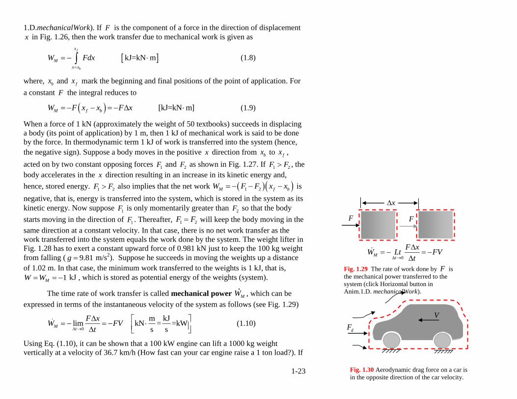
1.D.mechanicalWork). If F is the component of a force in the direction of displacement
x in Fig. 1.26, then the work transfer due to mechanical work is given as
kJ=kN m
f
b
x
M
x x
W Fdx
(1.8)
where, bx and fx mark the beginning and final positions of the point of application. For
a constant F the integral reduces to
[kJ=kN m]M f bW F x x F x (1.9)
When a force of 1 kN (approximately the weight of 50 textbooks) succeeds in displacing
a body (its point of application) by 1 m, then 1 kJ of mechanical work is said to be done
by the force. In thermodynamic term 1 kJ of work is transferred into the system (hence,
the negative sign). Suppose a body moves in the positive x direction from bx to fx ,
acted on by two constant opposing forces 1F and
2F as shown in Fig. 1.27. If 1 2F F , the
body accelerates in the x direction resulting in an increase in its kinetic energy and,
hence, stored energy. 1 2F F also implies that the net work 1 2M f bW F F x x is
negative, that is, energy is transferred into the system, which is stored in the system as its
kinetic energy. Now suppose 1F is only momentarily greater than
2F so that the body
starts moving in the direction of 1F . Thereafter, 1 2F F will keep the body moving in the
same direction at a constant velocity. In that case, there is no net work transfer as the
work transferred into the system equals the work done by the system. The weight lifter in
Fig. 1.28 has to exert a constant upward force of 0.981 kN just to keep the 100 kg weight
from falling ( 9.81g m/s2). Suppose he succeeds in moving the weights up a distance
of 1.02 m. In that case, the minimum work transferred to the weights is 1 kJ, that is,
1MW W kJ , which is stored as potential energy of the weights (system).
The time rate of work transfer is called mechanical power MW , which can be
expressed in terms of the instantaneous velocity of the system as follows (see Fig. 1.29)
0
m kJlim kN = =kW
s s
Mt
F xW FV
t (1.10)
Using Eq. (1.10), it can be shown that a 100 kW engine can lift a 1000 kg weight
vertically at a velocity of 36.7 km/h (How fast can your car engine raise a 1 ton load?). If
x
F F
0M
t
F xW Lt FV
t
Fig. 1.29 The rate of work done by F is
the mechanical power transferred to the
system (click Horizontal button in
Anim.1.D. mechanicalWork).
V
dF
Fig. 1.30 Aerodynamic drag force on a car is
in the opposite direction of the car velocity.
1-24
the external force is in the opposite direction of the velocity, the rate of work transfer
becomes positive, which is illustrated in the following example.
EXAMPLE 1-4 Power in Mechanics
The aerodynamic drag force in kN on an automobile (see Fig. 1.30) is given as
21
2000d dF c A V
where, dc is the non-dimensional drag coefficient, A is the frontal area in m2, is the
density of the surrounding air in kg/m3, and V is the velocity of air with respect to the
automobile in m/s. (a) Determine the power required to overcome the aerodynamic drag
for a car with 0.8dc and 25 mA traveling at a velocity of 100 km/h. Assume the
density of air to be 1.15 kg/m3. What-if scenario: (b) What would the power
requirement be if the car travelled 20% faster?
SOLUTION The car must impart a force equal to dF on its surroundings in the opposite
direction of the drag to overcome the drag force. The power required is the rate at which
it has to do (transfer) work.
Assumptions The drag force remains constant over time.
Analysis Use the unit converter daemon in TEST to verify that 100 km/h is 27.78 m/s.
Using Eq. (1.10), the rate of mechanical work transfer can be calculated as
3
3
1 m kJ kN = =k
49.
W2000 s s
0.8 5 1.15 27.78 31 kW
2000
M d dW F V c A V
What-if Scenario The power to overcome the drag is proportional to the cube of the
automobile speed. A 20% increase in V , therefore, will cause the power consumption to
overcome drag to go up by a factor of 31.2 1.728 or 72.8%.
Discussion The sign of the work transfer is positive, meaning work is done by the system
(the car engine). A gasoline (heating value: 44 MJ/kg) powered engine with an overall
efficiency of 30% will consume 13.45 kg of fuel every hour to supply 49.31 kW of shaft
power. This translates to 7.43 km/kg or 21 mpg (assuming a gasoline density of 750
Did you know?
Work is about 3 times more expensive than heat.
Because electricity can be converted into any type of work,
the price of work is equivalent to price of electricity. At
$0.10/ kW h , the price of 1 GJ of electric work is
$27.78.
A Therm of natural gas has a retail price of $ 1. The price of
1 GJ of heat, therefore, is $9.48.
r F
FrT
sh 260
NW T
Fig. 1.31 Power transfer by a rotating
shaft is very common in many
engineering devices (click on shW in
Anim.1.D. workTransferModes).
1-25
kg/m3) if the entire engine power is used to overcome drag only. Additional power is
required for accelerating the car, raising it against a slope, and overcoming rolling
resistance. At highway speed, the lion share of the power, however, goes into overcoming
the aerodynamic drag.
B. Shaft Work ( sh sh, W W )
Torque acting through an angle is the rotational counterpart of force acting through a
distance. Work transfer through rotation of shafts is quite common in many practical
systems – automobile engines, turbines, compressors, gearboxes, to name a few.
The work done by a torque T in rotating a shaft through an angle in radians
is given by F s Fr T (see Fig. 1.31 and click on shW in Anim.
1.D.workTransferModes). The power transfer through a shaft therefore can be expressed
as
sh0
kN mlim 2 =kW
60 st
T NW T T
t
, (1.11)
where, is the rotational speed in radians/s and N is the rotational speed measured in
rpm (revolution per minute). At 3000 rpm, the torque in a shaft carrying 50 kW of power
can be calculated from Eq. (1.11) as 0.159 kN m . Work transfer over a certain period
can be obtained by integrating shW over time. For a constant torque, shW is given as
sh sh 2 kW s=kJ60
NW W dt T t , (1.12)
Appropriate signs must be attached to these expressions based on the direction of work
transfer.
C. Electrical Work ( el el, W W )
When electrons cross a boundary, work is done because these charged particles are
pushed by an electromotive force. The familiar formula for electrical work
2 2
el
el el
kW ; 1000 W/kW 1000 W/kW 1000 W/kW
kJ ;
VI V I RW
R
W W t
(1.13)
R
110 VV 10 ampI
Fig. 1.32 Electrical heating of water involves work or
heat transfer depending on which boundary (the red or the
black) defines the system (click on elW in Anim.1.D.
workTransferModes).
in elW W
in inQ W
el
2
1000 W/kW
1000 W/kW
1.1 kW
VIW
V
R
0x
x bxx
F kx
fxx
Fig. 1.33 To elongate a linear spring,
the applied force has to be only
differentially greater than kx .
1-26
where, V is the potential difference in volt, I is the current in ampere, and R is the
resistance in ohm can be derived from the fundamentals of force time distance. Like shaft
work, electrical work is easy to identify and evaluate. Appropriate signs must be added to
these expressions depending on the direction of the energy transfer with respect to the
system. For instance, suppose the electric heater in Fig. 1.32 operates at 110 V drawing a
current of 10 amps. For the heater as a system, the electrical work transfer rate can be
evaluated as el 1.1W kW.
Sometimes there can be confusion between heat and electrical work transfer. For
instance, in the electrical water heater shown in Fig. 1.32, the water is commonly said to
be heated by electricity. To answer if this is a heat or work interaction, we must
remember to look at the boundary rather than the interior of the system. Accordingly, it is
el 1.1W kW for the system within the red boundary and 1.1Q kW for the system
defined by the black boundary. While the sign of the work or heat transfer clearly tells us
the direction of the energy transfer with respect to the system, system-specific symbols
need only the magnitude - for example, it is sufficient to state in 1.1W kW and in 1.1Q
kW in Fig. 1.32. However, we will prefer the algebraic quantities which can be directly
substituted into the balance equations to be developed in the next chapter.
D. Boundary Work ( , B BW W )
Boundary work is a general term that includes all types of work that involve
displacement of any part of a system boundary. Mechanical work, work transfer during
rigid body motion, clearly qualifies as boundary work. However, boundary work is more
general in that it can also account for distortion of the system. Work transferred in
compressing or elongating a spring is a case in point. For a linear spring with a spring
constant k (kN/m), the boundary work transfer in pulling the spring from a beginning
position bx x to a final position fx x (see Fig. 1.33) can be expressed as
2
2 2
2 2
ff f
b b b
xx x
B f b
x x x x x
x kW Fdx kxdx k x x
(1.14)
where, 0x is the undisturbed position of the spring. The negative sign indicate that
work has been transferred into the spring (the system). For a linear spring with a k of
200 kN/m, the work transferred to the spring by elongating it by 10 cm from its rest
position can be calculated from Eq. (1.14) as 1 kJ.
A
mg Apo
pA
Fig. 1.34 The system expands due to heat
transfer and raises the weights (click on
heating option in Anim.1.A. pressure).
.
A
mg Apo
pA
Fig. 1.35 Weights on the piston are
increased in small increments (try
different modes of compression in Anim.
5.A.pTsConstCompression).
1-27
The most prevalent mode of boundary work in thermal systems, however,
accompanies expansion or contraction of a fluid. Consider the trapped gas in the piston-
cylinder device of Fig. 1.34 as the system. Heated by an external source, the gas (system)
expands and lifts the load on top of the piston (Anim. 1.D.pdVExpansion). Positive
boundary work is transferred during the process from the system to the load. If the
heating process is slow, the piston can be assumed to be in quasi-equilibrium (no net
force) at all times, and a free body diagram of the piston (see Anim. 1.A.pressure) can be
used to establish that the internal pressure p remains constant during the expansion
process. Now suppose instead of heating the gas, the weight on top of the piston is
increased in small increments or chunks as shown in Fig. 1.35 (see Anim.
1.D.pdVCompression). Obviously, the pressure inside will increase as more weights are
added. However, if the chunks are differentially small, the piston can again be assumed to
be in quasi-equilibrium, allowing a free body diagram of the piston to express p in terms
of external forces on the piston.
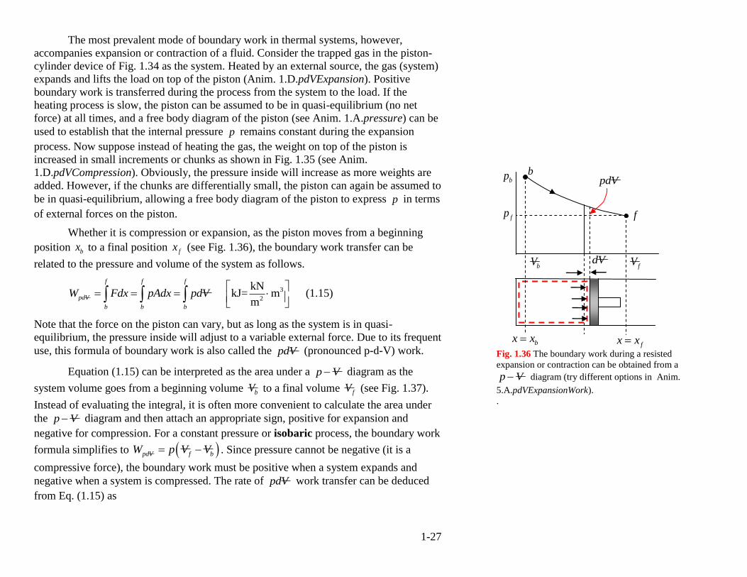
Whether it is compression or expansion, as the piston moves from a beginning
position bx to a final position fx (see Fig. 1.36), the boundary work transfer can be
related to the pressure and volume of the system as follows.
3
2
kN kJ= m
m
f f f
pdV
b b b
W Fdx pAdx pdV
(1.15)
Note that the force on the piston can vary, but as long as the system is in quasi-
equilibrium, the pressure inside will adjust to a variable external force. Due to its frequent
use, this formula of boundary work is also called the pdV (pronounced p-d-V) work.
Equation (1.15) can be interpreted as the area under a p V diagram as the
system volume goes from a beginning volume bV to a final volume fV (see Fig. 1.37).
Instead of evaluating the integral, it is often more convenient to calculate the area under
the p V diagram and then attach an appropriate sign, positive for expansion and
negative for compression. For a constant pressure or isobaric process, the boundary work
formula simplifies to pdV f bW p V V . Since pressure cannot be negative (it is a
compressive force), the boundary work must be positive when a system expands and
negative when a system is compressed. The rate of pdV work transfer can be deduced
from Eq. (1.15) as
bV dV fV
b bp
fp f
bxx fxx
pdV
Fig. 1.36 The boundary work during a resisted
expansion or contraction can be obtained from a
p V diagram (try different options in Anim.
5.A.pdVExpansionWork).
.
1-28
3
2
kN m kJ kW
m s s
pdV
pdV
dW dVW p
dt dt
(1.16)
In the absence of mechanical work, pdV work is the only type of boundary
work that is present in stationary systems (see Anim. 1.D.externalWork). In the analysis
of reciprocating devices such as automobile engines and certain types of pumps and
compressors, the pdV work plays an important role. Despite the high speed operation of
these devices, the quasi-equilibrium assumption and the resulting pdV formula produce
acceptable accuracy in the evaluation of work transfer.
EXAMPLE 1-5 Boundary Work During Compression
A gas is compressed in a horizontal piston-cylinder device. At the start of compression
the pressure inside is 100 kPa and volume is 0.1 m3. Assuming the pressure to increase in
inverse proportion to the volume, determine the boundary work in kJ if the final volume
is 0.02 m3.
SOLUTION Evaluate the pdV work using Eq. (1.15).
Assumptions The gas is in quasi-equilibrium during the process.
Analysis The pressure can be expressed as a function of volume and the conditions
during the beginning of the process ( 100bp kPa, 0.1bV m3).
3constant 100 0.1 10 kPa.m kN m kJb bpV p V
The boundary work, now, can be obtained by using Eq. (1.15)
0.02
0.1
10 0.0210 ln 10ln
016.09 k
.J
1
f f
B
b b
W pdV dV VV
Discussion The key to direct evaluation of the pdV work is to examine how p varies
with respect to V . In seeking a relationship between p and V , a free body diagram of
the piston (see Anim. 1.A.pressure) can be helpful in many instances.
EXAMPLE 1-6 Boundary Work During Expansion
constantpV
f
b
fp
p
bp
fV bV
const.
pV
Fig. 1.37 Schematic for Ex. 1-5
1-29
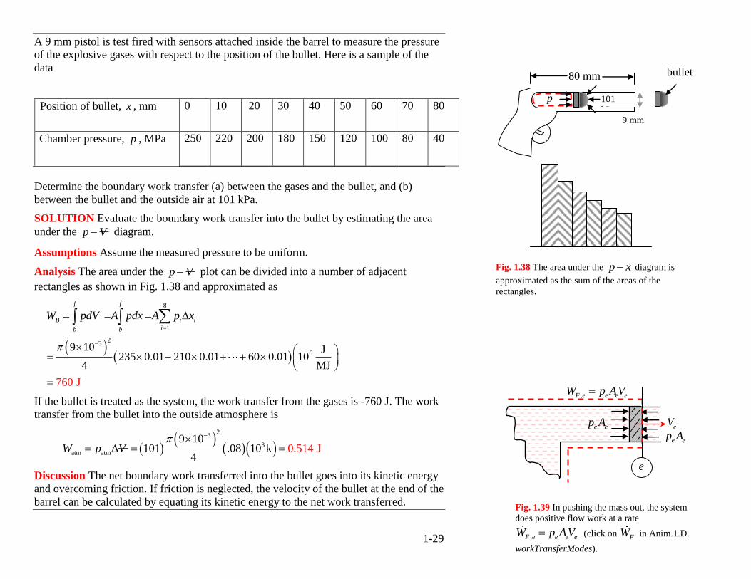
A 9 mm pistol is test fired with sensors attached inside the barrel to measure the pressure
of the explosive gases with respect to the position of the bullet. Here is a sample of the
data
Position of bullet, x , mm
0 10 20 30 40 50 60 70 80
Chamber pressure, p , MPa
250
220 200 180 150 120 100 80 40
Determine the boundary work transfer (a) between the gases and the bullet, and (b)
between the bullet and the outside air at 101 kPa.
SOLUTION Evaluate the boundary work transfer into the bullet by estimating the area
under the p V diagram.
Assumptions Assume the measured pressure to be uniform.
Analysis The area under the p V plot can be divided into a number of adjacent
rectangles as shown in Fig. 1.38 and approximated as
8
1
23
69 10 J
235 0.01 210 0.01 60 0.01 104
760
J
J
M
f f
B i i
ib b
W pdV A pdx A p x
If the bullet is treated as the system, the work transfer from the gases is -760 J. The work
transfer from the bullet into the outside atmosphere is
2
3
3
atm atm
9 10101 .08 10 0.5
414 JkW p V
Discussion The net boundary work transferred into the bullet goes into its kinetic energy
and overcoming friction. If friction is neglected, the velocity of the bullet at the end of the
barrel can be calculated by equating its kinetic energy to the net work transferred.
80 mm
9 mm
bullet
p
Fig. 1.38 The area under the p x diagram is
approximated as the sum of the areas of the
rectangles.
101
kPa
,F e e e eW p AV
e ep A
e ep A
e
e
eV
Fig. 1.39 In pushing the mass out, the system
does positive flow work at a rate
,F e e e eW p AV (click on FW in Anim.1.D.
workTransferModes).
.
1-30
E. Flow Work ( FW )
Consider the force balance on a thin element of fluid at a particular port, say, the exit port
e of an open system shown in Fig. 1.39 (Also, click on FW in Anim. 1.D.
workTransferModes). The element, which can be thought of as an invisible piston, does
not flow out on its own will, but is subjected to tremendous forces from both left and
right (see Fig. 1.39). For it to be forced out of the system, the force from inside should
only be differentially greater than the force from outside (to overcome the tiny friction as
the element rubs against the wall). If ep is the pressure at that port, the force on both the
faces of the element can be approximated as e ep A . Since the element is forced out with a
velocity eV , the rate at which work is done on the element can be obtained from Eq.
(1.10) as
2
, 2
kN m kJ m = =kW
m s sF e e e e e eW FV p AV
(1.17)
This is known as the flow work or, more precisely, the rate of flow work transfer at the
port. At the exit, the sign of the flow work is positive because work is done by the system
in pushing the flow out into the surroundings. Similarly, the flow work transferred at an
inlet is given by ,F i i i i i iW FV p AV , where the negative sign is added to indicate that
work is transferred into the system as external fluid is injected into the system.
In Sec. 1.2.4 we discussed why heat transfer through the port openings can be
neglected in open systems. Can we make the same assumption about the work transfer
through the inlets and exits of an open system? The rate of the flow work FW depends on
the product of pressure, velocity, and area of the flow, and cannot be summarily
neglected as none of these are necessarily negligible. If atmospheric air (pressure of about
100 kPa) enters a room through a 3 m 1 m door at a gentle speed of 3.33 m/s, the flow
work transfer can be calculated to be -1 MW, a power that is equivalent to turning on
1000 heaters each with a power rating of 1 kW. We don‟t feel this tremendous amount of
energy transfer through flow work because when the air leaves the room through a
window or another door (normally air breezes through a room only when there is a cross
flow), an almost equivalent amount of work is transferred from the room to the outside
surroundings leaving no significant amount of energy stored in the room. On the other
hand, when air enters an evacuated insulated tank (see Fig. 1.5d or Anim. 1.C.charging),
the flow work transferred by the incoming flow causes the stored energy to increase,
which is manifested in a temperature rise of air in the cylinder. Unlike shaft, electric, and
Fig. 1.40 While the shaft, electrical, and
boundary work transfer are apparent from
this system schematic, the flow work
transfer is more subtle.
i
elW shW
,F iW
BW
1-31
boundary work, flow work is invisible (see Fig. 1.40). We will exploit this invisibility of
flow work to bundle it with the stored energy transported by a flow in Sec. 1.3.4G.
1.2.7 Net Work Transfer ( ext, W W )
There are many other minor modes of work transfer such as work due to polarization or
magnetism and work transfer in stretching a liquid film that we have not covered.
Fortunately, an exhaustive knowledge of all these modes is not necessary for analyzing
most thermodynamic systems. Based on the different modes of work transfer discussed
thus far, a systematic classification for work transfer can be developed.
The net rate of work transfer out of a system can be split into various groups
(click on different terms in Anim. 1.D.workTransferModes) as shown in Fig. 1.41 and
expressed as
ext
ext sh el
: External Work : Boundary Work : Other Types
...
B O
F F B O F M pdV
W W W
W W W W W W W W W W W (1.18)
where, ext sh el BW W W W (1.19)
Basically, this equation separates total work into two major parts - flow work and
external work, extW . As we will see in the next chapter, flow work is absorbed in other
terms in the energy balance equation, leaving external work as the only relevant work
transfer in an energy analysis. External work can be seen to consist of boundary work,
which is the sum of mechanical and pdV work, and other work, which is the sum of
shaft, electrical, and any other type of work that may be present. In most analysis,
however, it is sufficient to express external work as the sum of boundary, shaft, and
electrical work.
To identify a specific type of work transfer, inspect the boundary and look for (a)
displacement of any part of the boundary for boundary work, (b) electric cables for
electrical work, (c) rotating shaft for shaft work, and (d) mass transfer for flow work. In
practical systems, only one or two of these modes may be present simultaneously. In
closed systems, for instance, the flow work, by definition, is absent.
EXAMPLE 1-7 Different Types of Energy Interactions
A gas trapped in a piston-cylinder device is subjected to the energy interactions shown in
the Fig. 1.42 for 30 seconds: The electric resistance draws 0.1 amp from a 100 V source,
Fig. 1.42 Different types of work
transfer in Ex. 1-7.
A
mg Apo
ip A
b
f
1-32
the paddle wheel turns at 60 rpm with the shaft transmitting a torque of 5 N m , and 1 kJ
of heat is transferred into the gas from the candle. The volume of the gas increases by 6 L
during the process. If the atmospheric pressure is 100 kPa and the piston can be
considered weightless, determine the net transfer of energy into the system.
SOLUTION Evaluate the different types of energy transfers during the process and add
them algebraically to find the net energy transfer.
Assumptions The piston is at mechanical equilibrium (no force imbalance) at all times.
Analysis Let us evaluate different modes of energy transfer treating the gas as the
system.
Boundary Work: During the expansion of the gas, boundary work transferred is
positive. To obtain a relation between ip and V , a free body diagram of the piston
yields
pistoni
mp A
0
0 piston 0 1000 N/kN
i
gp A p p
From Eq. (1.15), 0
f
B i f b f b
b
W pdV p V V p V V
3 3100 kPa 6 10 m 0.6 kJ
Shaft Work: From Eq. (1.12)
sh
60 52 2 30 0.94 kJ
60 60 1000
NW T t
Electrical Work: From Eq. (1.13)
el
100 0.1 kW 30 s 0.3 kW
1000 1000
VIW t
Heat Transfer: 1 kJQ (given)
The net work transfer can be summed up as
ext sh el 0.6 0.94 0.3 0.64 kJBW W W W W
Did you know?
To transfer enough sound energy to warm up
a cup of coffee, you have to yell continuously
for 8 years, 7 months and 6 days.
Fig. 1.43 How do you classify this
enjoyable interaction? Mass transfer,
of course.
1-33
This means that 0.64 kJ of work and 1 kJ of heat are transferred into the system.
Therefore, the net energy transfer into the system during the process is 1.64 kJ.
Discussion While evaluating a particular mode of work or heat transfer, it is an
acceptable practice to determine the magnitude first and then apply the sign convention to
add an appropriate sign based on the direction of energy transfer. The net energy
transferred into the system must give rise to an increase in the stored energy. Kinetic and
potential energies of the system remaining unchanged, the transferred energy must be
stored in the internal energy of the system.
1.2.8 Other Interactions
Are there other interactions between a system and its surroundings besides mass, heat and
work interactions? What about microwaves, radio waves, laser, sound waves, nuclear
radiation, or, for that matter, the scent of a perfume? On closer examination, it can be
established that none of these interactions are fundamentally new; they are special cases
of heat or mass transfer. We can, therefore, conclude that mass, heat, and work
interactions, summarized in Anim. 1.C.genericTransfer, are sufficient to capture all
thermodynamic activities between a system and its surroundings. The lack of mass
transfer makes a system closed, the lack of heat transfer makes it adiabatic, and the lack
of all interactions makes a system isolated (Anim. 1.C.systemTypes). Classification of
systems based on interactions will play an important role in the chapters ahead.
1.2.9 Consequences of Interactions
Interactions have their consequences. If hot water is added to cold water in a bathtub, the
addition of hot water not only increases the system mass but also its stored energy as
evident from a temperature rise. When heat is added to a system, we expect its
temperature to rise, but this is not always so. A glass of ice-water mixture does not warm
up to room temperature despite heat transfer from the surroundings until the last chunk of
ice melts. Heat transfer in this case is responsible for a change of phase. Work transfer
can also bring about the same changes as heat transfer can. Figure 1.44 shows three
different ways of heating a gas using electric, shaft and boundary work transfer. While
the temperature rise can be readily attributed to Joule heating from electrical work and
viscous friction from the paddle-wheel work driven by the shaft, we are not accustomed
to changes involving boundary work. Bicyclists must be familiar with a hand pump
heating up when inflating a tire. In fact, this rise in temperature through boundary work
transfer is utilized to auto-ignite diesel as it is sprayed into the compressed air in the
cylinders of a diesel engine, eliminating the need for spark plugs. Sometimes, a system
Fig. 1.44 Different types of work
transfer bring about an increase in
the temperature of air.
shW
elW
BW
1-34
may spontaneously change without any interactions at all, as in the case of an isolated
explosive mixture or the mixing between ink and water after they are isolated in a tank
(see Anim. 1.C.isolatedSystem).
A major goal of thermodynamic analysis is to predict how a system transforms
spontaneously or when prodded through interactions with its surroundings. Conversely,
given the changes in the system, an analyst maybe interested to determine the precise
interactions that led to those changes. Either way, thermodynamic analysis requires
changes in a system to be quantitatively described.
1.3 States and Properties
A system is quantitatively described by its states and properties.
A state is a mathematical description of the condition of a system or a flow at a given
time expressed as a set of properties, which are measurable characteristics or attributes
of the system or the flow.
To explore the meaning of these thermodynamic terms, consider a system made of a gas
trapped in the piston-cylinder device of Fig. 1.45. Assume that the system is uniform, that
is, there is no significant variation of properties across locations within the system. The
particular condition of the system at a given time can then be described by a single state,
say, state-1 (states are usually designated by roman numerals or indices), consisting of a
set of properties such as mass 1m , volume 1V , pressure 1p , temperature 1T , elevation 1z ,
etc. Implicit in this description is the assumption that the system is in equilibrium.
Thermodynamic equilibrium and its role in evaluating a state will be discussed in Chapter
3 as well as Chapter 11. Simply put, a system is said to be in thermodynamic
equilibrium when, blocked from all interactions, all its internal activities – internal
motion, heat transfer, chemical reaction – spontaneously subside. For example, if a
system composed of a fixed amount of liquid water and ice is isolated (see Fig. 1.46),
some ice may melt or some water may freeze until the mixture comes to an equilibrium
from which point water and ice coexist at the same state as long as there is no further
interactions with the surroundings. If interactions are temporarily allowed to occur with a
system in equilibrium and then the system is isolated again, it will seek a new equilibrium
defined by a new set of properties. If the gas in Fig. 1.45, described by state-1, is
suddenly isolated (click Isolate in Anim. 1.E.globalEqulibrium) its properties such as
temperature and pressure will not change over time if state-1 was in thermodynamic
equilibrium to start with. However, if the piston is displaced to a new position, the system
will go to a new equilibrium (given enough time). Properties that describe an equilibrium
Fig. 1.45 The condition of the gas
is represented by the system state
state-1 at a given time (see Anim.
1.E.extendedStates).
1 1 1, ,p T m
State-1
Fig. 1.46 Ice and water co-exist in equilibrium
when isolated from the surroundings. At
equilibrium, all internal imbalances disappear
and thermodynamic properties assume fixed
values unique to that equilibrium (see Anim.
1.E.globalEquilibrium).
1-35
are called thermodynamic properties and the set of thermodynamic properties
constitute a thermodynamic state (see Anim. 1.E.thermodynamicState).
A complex system may not always be in equilibrium. There can be change in
properties across locations or over time or both. However, such a non-uniform unsteady
system can be broken into small chunks called local systems, each of which can be
assumed to be in its local thermodynamic equilibrium or LTE . A non-uniform system,
therefore, can be expressed as a collection of local systems in equilibrium. Similarly, an
unsteady system that evolves over time can be thought of as a system passing through a
succession of equilibriums (see Anim. 1.E.localEquilibrium). Without the assumption of
LTE, a mathematical description of a system becomes almost unmanageable.
The uniform state of Fig. 1.45 can be assumed to represent a particular
equilibrium of the system. For practical analysis, however, the description of a system
may extend beyond the description of the underlying equilibrium state. An extended
state (see Anim. 1.E.extendedState) includes properties such as system volume, total
mass, system velocity, etc., which do not necessarily affect the underlying equilibrium.
For example, if the system of Fig. 1.45 is raised to a different elevation, the potential
energy of the system will change without affecting the equilibrium state. Potential
energy, therefore, can be part of an extended state, but not a core property of equilibrium.
Such an extended state that completely describes a system enclosed by a boundary is
called a system state. Two different system states can have the same underlying
thermodynamic state. However, if the gas in Fig. 1.45 is compressed by the piston to a
new state, state-2, the underlying equilibrium state is also changed. The change in a
property, say, pressure, can be obtained from the two system states as 2 1p p p .
In describing the mass interactions that occur in an open system, it is
necessary to describe a flow at the inlet and exit ports. If a port is selected slightly away
from the system, the flow can be assumed uniform. Moreover, if a little lump of fluid is
suddenly isolated, say, at the inlet of the turbine in Fig. 1.47, the thermodynamic
properties ip , iT , etc., would not change with time; that is, the flow can be assumed to be
based on a local thermodynamic equilibrium (LTE) at the inlet. A uniform flow,
therefore, can be described by a flow state that builds upon the local equilibrium state by
adding properties such as flow area, flow velocity, mass flow rate, etc. The inlet and exit
states, state-i and state-e in Fig. 1.47, are such flow states based on LTE. The change in a
property, say, pressure, between the exit and inlet state can be obtained from the two flow
states as e ip p p .
i
, ,i i im p T
shW
e , ,e e em p T
Fig. 1.47 The inlet and exit conditions are
defined by two flow states, which build upon the
underlying equilibrium states at the inlet and exit
ports (click on Flow State in Anim.
1.E.extendedStates).
, i ip T
1-36
As already mentioned, the set of variables that constitute a state are called
properties (see Anim. 1.E.property). We have already come across several properties
such as mass, pressure, temperature, velocity, etc. To be a property, first and foremost, a
variable must describe some aspect of a state. Mass, velocity, and temperature are
properties because they describe a system state. Similarly, mass flow rate, velocity, and
temperature are properties of a flow state. However, work and heat transfer are not
properties because they describe interactions, not a state.
Second, a property is without memory. In mathematical terms, it is a point
function, which means that its value does not tell us anything about the history of a state.
When the temperature of a uniform system is measured as 100 o C , we can never tell
whether the system was heated or cooled to achieve the current temperature. If a system
migrates from state-1 to state-2, we can write 2 1T T T simply from the knowledge of
the two states, ignoring the specific path followed by the system. When the two states are
infinitesimally close, T dT , which is known as an exact differential. Heat and work
transfer, on the contrary, are path functions since their values depend on precisely how
the system transitions from one state to another. To underscore the fact that a path
function cannot be a property, its differential, known as an inexact differential, is
expressed with a crossed d – dQ or dW , for example, is fundamentally different from
dT or dp in that while the latter can be expressed as a difference the former cannot.
In our lake analogy, the water in a lake (stored energy) is a property since any
change in the total amount of water in a given period can be determined from the water
levels at the beginning and end of the period. However, the rainfall during that time,
analogous to heat transfer during a process, is a path function since it needs continuous
monitoring.
Finally, different properties can be combined to create new properties for
analytical convenience. Since mass and volume are properties (they describe a system,
and they are point functions), we must accept their ratio density and its inverse,
specific volume 1/v , as legitimate properties. Summarizing, a variable can be
considered a property if it (a) represents an attribute of a state, (b) is a point function, or
(c) is a combination of other legitimate properties.
Given that a uniform system or flow can be described by an extended system or
flow state, a non-uniform system can be described by decomposing into a large number
of uniform subsystems. For example, the non-uniform system of Fig. 1.50 - a solid block
submerged in water – can be represented by two system states describing the solid and
liquid subsystems. The state of such a composite system is called the global state, which
State-2
State-1
Fig. 1.48 The global state of a non-uniform
system can be described by the (local) states
of the subsystems (see Anim.
5.B.blockInWater).
1-37
consists of an aggregate of the states of its subsystems. When properties vary in a
continuous manner throughout a system, the local subsystems have to be quite small.
Assuming local thermodynamic equilibrium (LTE) at each local system, the global state
can be described by the collection of the local states. To answer how small a local
system can be, an understanding of the macroscopic nature of classical thermodynamics
is necessary.
1.3.1 Macroscopic vs. Microscopic Thermodynamics
Consider a particular instant during the charging of an empty cylinder with propane,
which comes from a supply line with constant properties as shown in Fig. 1.49. Suppose
we are interested in the density of the propane inside the tank (the system) at any instant.
For the local system drawn around point A in this figure, the density can be expressed as
3
kg
mA
m
V
(1.20)
where, V is the volume and m is the mass of the sub-system. For a non-uniform
system, A obviously depends on the size V of the sub-system, and assumes the
average value when V approaches the total volume V of the tank (see Fig. 1.50). On
the other hand, as V is made smaller around location A, it approaches a fairly constant
value local,A reflecting the density at the local level. Similarly, B , the density calculated
around point B, approaches a different local value local,B . The volume axis in Fig. 1.50 is
actually in a logarithmic scale and shows that local limits are approached long before
V approaches zero. As a matter of fact, when V truly approaches zero, we reach the
molecular scale, explaining the wild fluctuation of density. As a matter of fact, classical
thermodynamics is based on the hypothesis that a working substance can be treated as a
continuum regardless of the scale of the system. That is, a system, no matter how small,
is assumed to consist of such a huge collection of constantly interacting molecules that its
behavior can be explained without any reference to molecular dynamics.
As long as V is large enough to contain a huge number of molecules and the
time of measurement is sufficiently large to allow a huge number of interactions among
the molecules, the continuum hypothesis is applicable. To have an idea about what is a
sufficiently small volume and what is sufficiently large duration, consider a local state of
air under room conditions having a tiny volume 31 mV . Using kinetic theory, it can
Alocal,
Blocal,
A
V
avg
V
Fig. 1.50 Density approaches the local
limit as V becomes small.
B
Breakdown of
the continuum hypothesis.
Local limits
Propane 3 8C H
A
B
Fig. 1.49 As propane enters the
tank, the local states at point A
may be slightly different from that
at B because the system is not
truly uniform.
1-38
be shown that even such a small system will consist of billions of molecules with trillions
of collisions occurring every microsecond. Similarly, when the change of a state is
tracked over time, the concept of properties such as temperature or pressure breaks down
as we approach a true instant. However, a microsecond is probably long enough to have
sufficient number of collisions for local properties to assert their values.
The macroscopic view of classical thermodynamics is based on the continuum
hypothesis. Although mathematically a continuum extends to zero volume at any given
instant of time, we will use the terms macroscopic point to indicate the minimum
acceptable size of a local system (about a micrometer or even smaller) and a
macroscopic instant (about a microsecond or even smaller) as the minimum duration
necessary for the microscopic particles to exchange meaningful information. For an
overwhelming majority of engineering systems, including micro mechanical systems, this
viewpoint works well, and seldom there is any need for spatial resolution below a
macroscopic point or time resolution smaller than a macroscopic instant. Notable
exceptions, where the continuum assumption breaks down, include reentry of space crafts
through rarefied atmosphere and shock waves where steep changes in properties occur
within distance comparable to molecular scales.
It should be mentioned that a parallel treatment of thermodynamics from a
microscopic view is adopted in statistical thermodynamics, where every system, large or
small, is treated as a collection of discrete particles, i.e. molecules or atoms. Laws of
macroscopic thermodynamics can be deduced by suitable averaging of molecular
phenomena. In this book, however, we will adopt the macroscopic framework, and only
occasionally discuss the underlying microscopic structure when it helps us understand
certain macroscopic behavior of a working substance.
1.3.2 An Image Analogy
Just as we used the lake analogy to visualize energy, heat, and work, we will develop the
image analogy to visualize different types of states introduced so far.
Consider a digital video of a flickering flame, which represents a non-uniform
time-dependent (transient) system. One of the frames from that video at a given instant
1t t is sketched in Fig. 1.51. An image such as this represents the global state of a non-
uniform system at a given time. Each pixel, in this case, behaves like a local system, its
state (composed of pixel color and brightness) being analogous to the local system state.
The resolution of the image is the size of a single pixel – analogous to the size of a
Pixel
Boundary
Image
Boundary
Fig. 1.51 A frame from a digital video
of a flickering flame represents a global
system state.
Systems
Closed
Steady Unsteady
Open
Steady Unsteady
Fig. 1.52 A simple classification of systems
based on mass interaction and whether the
global state changes over time (see Anim.
1.E.systemsClassified).
.
1-39
macroscopic point. The minimum exposure time necessary to record an image (a truly
instantaneous image is impossible as zero photons will be captured by the camera) in this
analogy corresponds to a macroscopic instant.
Due to the fact that thermodynamic systems are three dimensional, it would be
impossible for a simple camera to capture its global state. However, we can imagine a
state camera that records the distribution of local states in a three dimensional video. As
a matter of fact, sophisticated visualization software routinely use false colors to
represent field variables gathered through experiments or numerical analysis.
The image analogy can be used to classify systems into different categories (see
Fig. 1.52 or Anim. 1.E.systemsClassified). A system, whose global state changes with
time is called an unsteady system – the flickering flame in that sense is an unsteady
image. A steady system, on the other hand, does not change its global state over time,
which means that the local states comprising the global state remain frozen in time. In
our image analogy, the digital video of the system reduces to a single frozen image.
Global properties such as the total stored energy or mass of a system, therefore, remain
constant for a steady system. Systems, open or closed, steady or unsteady, can be uniform
or non-uniform based on the absence or presence of spatial variations of local states. A
uniform system can be represented by a single color shared by all pixels since all local
states of a uniform system are identical. Note that a uniform system can be transient so
that the color of the image may continually change over time. This simple classification
will form the basis of simplification of governing equations to be developed in the next
chapter..
1.3.3 TEST and the State Daemons
State daemons in TEST are the building blocks of all other daemons. With the look and
feel of a graphical spread sheet, these daemons are used for evaluating extended states of
uniform systems and uniform flows for a wide range of working substances. State
daemons are divided into two categories, system state daemons and flow-state daemons,
which are located in Daemons> States> System and Daemons> States> Flow page
respectively. These pages can also be directly accessed from the Map. Both kinds of
daemons are sub-divided according to the material models used to classify the working
substances (these models will be our topic of discussion in Chapter 3). Thus, to find a
state involving a solid or a liquid we may use the SL (solid/liquid) model, for a gas the IG
(ideal gas) model, and for a fluid that may undergo phase transition (steam, for instance)
the PC (phase-change) model.
1-40
In this chapter, we will use some of the state daemons as a numerical laboratory to
explore the behavior of different properties of state to be introduced in the next section.
To illustrate some frequently used features of a state daemon, let us launch a particular
daemon, say, the SL flow-state daemon, by following the Daemons or Map links from the
TEST task bar. The daemon itself appears2 in a rectangular box (see Fig. 1.53). The
message panel at the top is followed by a global control panel. Buttons such as Super-
Calculate or Super-Init in the global control panel affect the entire solution. Hovering the
pointer over any widget brings up its definition on the message panel, which also displays
error messages and helpful tips on the message panel during calculations. Depending on
the selected tab, either the state panel or the I/O panel is displayed below the global
control panel.
The first row of the state panel is the state control panel, which is used to pick a
state number, select a working substance, initialize and calculate the state, and produce a
variety of thermodynamic plots. A set of properties, sixteen in this case, constitute the
complete system state. Each property is encapsulated in a widget, consisting of a
checkbox used to toggle between the input and display mode, a unique symbol with the
state number as the suffix, a field for displaying its value, and a drop-down menu for
selecting a unit. A property can be entered by clicking its checkbox and then typing in a
value and selecting an appropriate unit. When the Enter key or the Calculate button is
pressed, the property is read and the state is updated based on the current entries. To edit
or change a property, the checkbox should be clicked twice to enter the input mode.
Properties are color coded according to the classification to be discussed in Sec. 1.3.5.
Evaluating a state consists of three steps: identify the state by selecting a state number,
picking a working substance, entering the known (independent) properties, and clicking
the Calculate button (or the Enter key).
As an exercise, let us select water(L) as the working fluid, and evaluate state-1 for
the following conditions: p1=10 atm, T1=50 deg-C, and Vol1=100 gallons. Note
that the entire state, not just a particular property we may be interested in, is calculated at
once. If we try to enter an additional property, say, m1, the daemon will produce a
warning. While evaluating additional states, algebraic equations should be used to relate
properties. Vol2, for instance, can be entered as „=2*Vol1‟, provided state-1 is already
calculated. The I/O panel can be used as a calculator that understands evaluated
properties. For instance, the kinetic energy in kJ of a system at state-1 can be calculated
in the I/O panel by entering ‘=m1*Vel^2/2000‟. Now suppose we have evaluated a
number of states, each related to temperature at state-1, for a given working fluid. We can
2 In case your browser does not display the daemon, read the Getting Started section of the Tutorial
thermofluids.net
1-41
use T1 is a parameter in a what-if study by simply changing T1 to a new value and
clicking the Super-Calculate button on the global control panel to update all calculated
states. Likewise, to use the working fluid as a parameter, simply select a new fluid and
click Super-Calculate. To preserve the first set of calculations, a better approach is to
select a new case, say, Case-1, and then change the fluid and Super-Calculate. Just as a
collection of properties are stored in a state, a collection of states are stored in a case. The
daemon thus can generate property data for a series of states belonging to different fluids
with each series stored as a unique case. Selecting a calculated state or a calculated case
(identified by the @ sign), loads the state or the entire case. The Super-Calculate button is
also used to convert the unit system of an entire solution, to produce a detailed output of
the solution including spread sheet friendly tables in the I/O panel, and generating TEST-
codes (to be discussed later) for storing and reproducing the solution.
1-42
Fig. 1.53 A screenshot of the flow-state daemon (SL-model) with the state panel in the foreground and the I/O panel
behind.
1-43
Open a separate browser window and launch the flow-state daemon with the SL model
and compare the flow-state daemon with the flow-state daemon. The system mass (m) is
replaced by mass flow rate (mdot); the volume (Vol) is replaced by the volume flow rate
(Voldot). However, most of the core properties (marked in red, green, and blue) are
identical between the two types of states. To learn more about the state daemons, visit the
Tutorial> Daemons page.
1.3.4 Properties of State
We have already used several properties in discussing equilibrium and extended states.
This section will be devoted to a formal introduction of important properties that
constitute the bulk of an extended system or flow state. Keeping in mind that a
comprehensive evaluation of properties has to wait until Chapter 3, we will employ
suitable state daemons to develop a quantitative understanding of properties whenever
necessary.
The equilibrium state forms the core of an extended state and, therefore, it is
important to delineate thermodynamic properties from the rest. By definition, any change
in thermodynamic properties signals a change in the equilibrium of a system. If the
temperature of an ice-water system in equilibrium is increased by transferring heat, the
system will move into a new equilibrium described by a new set of thermodynamic
properties. An extended state that describes a system or flow beyond its core equilibrium
contains many other convenient properties. Material properties such as molar mass
depend only on the identity of the working substance and can be regarded as material
constants. Material and thermodynamic properties are intrinsic to a system (see Anim.
1.E.intrinsicProperty), they do not depend on whether they are measured by an observer
inside or outside the system. Extrinsic properties such as kinetic energy, on the other
hand, depend on the reference frame of the observer. A moving observer may not agree
with the values of such properties with a stationary observer. A change in an extrinsic
property may not affect the underlying equilibrium of a system – if the ice-water system
in our example is moved to a different elevation, its potential energy will change without
disturbing the equilibrium between the two phases of water. Extensive properties (see
Anim. 1.E.extensiveProperty) such as mass or stored energy of a system scale with the
extent of the system and are additive. For example, if two identical systems are
concatenated, extensive properties will double, but the equilibrium will not be disturbed.
As we introduce further properties of the system and flow states in this chapter, we will
classify them into categories as illustrated in Aim. 1.E.propertyGroups. This
classification will be helpful when we set out to evaluate an extended state of various
working substances in a comprehensive manner in Chapter 3.
Did you know?
The peak thrust generated by a turbofan
engine that propels a Boeing 747 is about
300 kN per engine.
A 2 million kg space shuttle needs a
minimum thrust of 19,620 kN for lift off
(can you calculate that?).
Did you know?
The mass of the smallest known particle,
the up quark, is 395.34 10 kg.
The mass of the observable universe is
estimated as 523 10 kg.
1-44
A. Properties Related to System Size ( , , , , , , V A m n m V n )
Several properties characterize the size or extent of a system or flow. Volume V of a
system (the symbol V is reserved for velocity) and cross-sectional area A of a flow are
geometrical attributes that can used to describe the extent of a system or a flow. Thus, the
volume of a piston-cylinder device or the exit area of a nozzle qualifies as an extensive
property of a corresponding system or flow state.
Mass m is a property that measures the quantity of matter in a system in kg in SI
and in lbm in English units. When we say a system is massive or heavy, we usually mean
that the weight (the force with which earth pulls the system) is large. Unlike weight, the
mass of a closed system stays the same regardless of elevation. It is easier to intuitively
understand force; hence, mass can be operationally defined by Newton‟s second law in
terms of force F and acceleration a .
2
m kN kN=kg.
1000 N/kN s N
maF
(1.21)
The weight w of a mass m , that is, the force with which the earth pulls an object of mass
m , can be related to the acceleration during a free fall or the acceleration due to gravity
g as
2
m kN kN=kg.
1000 N/kN s N
mgw
(1.22)
To prevent a free fall, an upward force w , proportional to the mass of the body, must be
exerted on the body. This gives us an appreciation for the mass of the body (see Anim.
1.A.weight). In space, mass can be appreciated in attempting to alter the inertia of a body
– the more massive the body, the greater is the force necessary to affect the magnitude or
direction of its velocity (think how we can distinguish two identical looking baseballs of
two different masses in the absence of gravity).
The acceleration due to gravity can be regarded as a proportionality constant
between the weight and mass of a system, which can be expressed by Newton‟s law of
universal gravitation in terms of the distance of the system from the center of the earth
and the gravitational constant. The local value of g therefore is a function of elevation z
of a system. At 45 degree latitude and sea level ( 0z ), it has a value of 9.807 m/s2.
Most engineering problems involve only minor changes in elevation compared to the
radius of the earth, and a constant value of 9.81 m/s2 for g , called the standard gravity,
mgw
Fig. 1.54 Although equal and opposite forces act
on the apple and earth, the acceleration of earth is
negligible while that of the apple is g .
1-45
provides acceptable accuracy. In this book we will assume standard gravity value for g
unless mentioned otherwise.
Beside mass, the amount of matter in a system can be expressed by another
extensive property called mole, which is a count of the smallest microscopic units that
constitute the system (see Anim. 1.F.massVsMole). Often that smallest unit is a molecule
for a pure substance, but sometime it can be an atom (in the case of a metal for instance)
or even electron or photon. To simplify the terminology, we will use the term molecule to
describe the smallest unit of a system. Given their huge numbers, a large unit called a
kmol (kilo-mol) is used in SI units to express the mole of a system. A kmol is much
bigger than a dozen: 1 kmol = 1000 mol, where a mol is precisely 236.023 10 , which is
known as Avogadro‟s number (note the spelling - a mole is a property while mol or kmol
is its unit). In English unit, the mole unit is 262.737 10 and is called a lbmol. The
symbol used to represent the mole of a system is n . Some properties of a state are
expressed on the basis of unit mass or unit mole of a working substance. Properties based
on mole are called molar properties, marked by a bar on top of their symbols. In Table
D-2 for example (tables are linked from the task bar in TEST), you will find several
molar properties of hydrogen with units such as kJ/kmol, kJ/(kmol.K), etc.
If the molecules comprising a system are identical, the ratio of the mass m to the
mole n , that is, the mass per unit mole must be a constant for a given working substance.
It is called the molar mass M (MM in TEST).
kg kmol
; Therefore, kmol kgkmol kg
m mM n
n M
3 (1.23)
Oxygen has a molar mass or 32 kg/kmol, which means that the mass of 1 kmol of oxygen
is 32 kg. Molar masses of several common substances are listed in Tables A-1, A-2 and
Table C-1. Most state daemons display the molar mass as soon as the working substance
is selected. Note that while in chemistry molar mass is understood as a ratio, the relative
mass of a molecule compared to oxygen atom, in engineering thermodynamics it is
regarded as a material property of the working substance with well defined unit. Even for
a homogenous mixture such as air, Eq. (1.23) can be used to define an average molar
mass, which turns out to be 29 kg/kmol for air. Given the molar mass of a substance, Eq.
(1.23) can be used to convert the amount of a system from mass to mole and vice versa.
3 Symbol is used to indicate a definition.
2H 2 kg/kmolM
2H O 18 kg/kmolM
2N 28 kg/kmolM
2O 32 kg/kmolM
Air 28.97 kg/kmolM
2CO 44 kg/kmolM
Fig. 1.55 Molar mass of a few common
gases (see Anim. 1.F.massVsMole).
Did you know?
The densest naturally occurring substance on
Earth is Iridium, at about 22,650 kg/m3.
Density of water is about 1000 kg/m3.
Density of air at sea level is about 1.229
kg/m3.
1-46
We have already come across mass flow rate m and volume flow rate V
expressed by Eqs. (1.2) and Eq. (1.1) while discussing mass interactions in Sec. 1.2.1.
These are properties of a flow and, therefore, members of the flow state (mdot and
Voldot in TEST). The amount of matter transported by a flow can also be expressed on
a molar basis, which is called the mole flow rate represented by the symbol n . An
expression for n can be derived by converting the mass in the shaded region that crosses
a given cross-section (see Fig. 1.8) in a unit time into mole.
kmol kg kmol
; s s kg
m AVn
M M
(1.24)
While , ,V m and n are relevant to a system state, , ,V m and n qualify a flow
and, hence, belong to a flow state. They are all extensive properties because merging two
identical systems or flows would double these properties. Although n or n do not
explicitly appear as part of the state panel, they can be calculated in the I/O panel using
expressions such as „=m1/MM1‟ or „=mdot1/MM1‟.
In the next chapter, we will introduce the conservation of mass principle, a
fundamental law of physics, in the form of a mass balance equation to track the inventory
of mass for a very general system. The mass equation will be used in almost all
subsequent chapters as we analyze a variety of practical thermodynamic systems.
B. Density and Specific Volume ( , v )
Density is a familiar property that expresses the concentration of matter, defined as
the mass per unit volume of the working substance.
3
kg
m
m
V
(1.25)
For most solids and liquids, density does not vary much - for instance, density of water is
about 1000 kg/m3 under atmospheric conditions and increases by only about 0.5% at 100
atm (at room temperature). A material is called incompressible if its density can be
regarded as a constant. While solids and liquids are often modeled as incompressible,
gases and vapors are compressible since their density can change drastically with changes
in pressure and temperature.
A more convenient property for thermodynamic analysis is specific volume v ,
defined as the volume of a substance per unit mass, which is the reciprocal of density.
1-47
The corresponding molar property is the molar specific volume v , defined as the
volume per unit mole.
3 31 m m
; ;kg kmol
V V VMv v vM
m n m
(1.26)
Note the consistent use of the bar, even in the symbol for molar mass, to emphasize a
mole based property. Also note the use of the term specific, which will be consistently
applied to properties that are based on a unit mass or unit mole of the working substance.
While v and v are specific properties (see Anim. 1.E.specificProperty), is not. Both
v and , however, are independent of the system size. Such properties are called
intensive properties and are generally represented by lower-case symbols. Pressure p
and temperature T (symbol t is reserved for time) also must be intensive since
concatenating two identical system does not change their values. For a compressible
substance (say, air), v and can also be regarded as thermodynamic properties since
they can be used to define an equilibrium. For an incompressible substance (say, a copper
block) they remain constant and can be regarded as material properties.
Another property that is related to density is relative density water/ (water at
some standard condition) , a dimensionless quantity which is also known as specific
gravity. Specific weight is another related property that is defined as the weight of an
unit volume of the material, which is simply g from Eq. (1.22). These properties,
however, are seldom used in thermodynamics in favor of specific volume and density.
Density of several solids and liquids are listed in Tables A-1 and A-2. In daemons based
on the SL (Solid/Liquid) model, density (rho) and specific volume (v) widgets are
populated as soon as a working substance is selected.
EXAMPLE 1-8 Mass vs. Mole
Determine (a) the mass (in kg) and mole (in kmol) of a 1-m3 block of aluminum. What-if
Scenario: (b) what would the answers be if the block were made of iron instead?
SOLUTION Obtain the molar mass of the working substance from Table A-1 or any SL
state daemon and evaluate the amount in mass and mole.
Analysis For aluminum (Al) Table A-1 lists Al 2700 kg/m3 and Al 27M kg/kmol.
The mass of the block can be obtained from Eq. (1.25) as
kmol 100
kg 2700
m 1 3
n
m
V
Aluminium
31 m
7840 kg
140.4 kmol
V
m
n
Iron
Fig. 1.56 The iron block is heavier because its
molecules (atoms) are heavier and more densely
packed compared to aluminum.
Did you know?
30 m/s is about 67 mph.
Typical velocity of a Jumbo jet is 250 m/s.
Altitude of flying for a Boeing 747 is 12 km.
Voyager 1 is currently traveling in deep space
away from the solar system at 17.4 km/s.
Particle beam accelerator has achieved near light
speed for atoms and molecules.
Radius of earth is 6378 km.
Height of Mount Everest is 8847 m.
Average depth of Pacific ocean is 4300 m.
1-48
Al Al Al 2700 1 2700 k gm V
The mole of aluminum can be found using Eq. (1.23) as
AlAl
Al
2700100 kmols
27
mn
M
TEST Analysis Launch the SL flow-state daemon located in Daemons> States> System
page. Select Aluminum (Al) from the material selector, enter the volume in appropriate
unit, and press the Enter key or the Calculate button. The mass m1 is calculated as 2700
kg. In the I/O panel, evaluate the mole from the expression „=m1/MM1‟ as 100.07
kmol.
What-if Scenario Select Iron (Fe) from the working substance selector, which updates
all properties automatically. The new answers can be founds as 7840 kg and 140.38kmol
respectively. Compared to aluminum, the same volume of iron has about 40.3% more
molecules.
DISCUSSION The mass flow rate of Ex. 1-2 can, similarly, be converted to mole flow
rate by applying Eq. (1.24). Since 2H O 18M kg/kmol, the mole flow rate is given as
2H O/n m M 39.13/18 2.17 kmol/s.
C. Velocity and Elevation ( , V z )
The instantaneous velocity V of a uniform system, say, a projectile, describes the state of
its motion and, therefore, is a legitimate system property. It is also an important
characteristic of a flow and, hence, a flow property. For non-uniform systems, the
distribution of velocity among the local state is known as the velocity field in fluid
mechanics. Even at local level, the velocity is a macroscopic property of the continuum
and should not be confused with disorganized microscopic motion of molecules.
The elevation or height z of a system is the vertical distance of its center of
gravity from an arbitrarily chosen horizontal level called the datum ( 0z ). The
standard datum is sea level. We will shortly discuss kinetic and potential energies, which
are derived properties from velocity and elevation. Since these properties depend on the
frame of reference of the observer, they are extrinsic. Note that changes in extrinsic
properties do not necessarily reflect a change in equilibrium (see Anim.
1.E.intrinsicProperty).
Ap
Fig. 1.57 Pressure at a point or the local
thermodynamic pressure.
1,gage 1 0p p p
2,vac 0 2p p p
1p
0p
2p
0
Vaccum
pressure
Gage
pressure
Fig. 1.58 Gage and vacuum pressure
depend on local atmospheric pressure.
Atmospheric
pressure
1-49
D. Pressure ( p )
Pressure p is the normal compressive force exerted by a fluid per unit area of a surface.
We experience these compressive forces underwater or when we go outside on a very
windy day. Pressure has the same unit as stress in mechanics - kN/m2 or kPa (kilo-Pascal)
in SI, and psi (lbf/in2) in English units. Other units in common use include MPa (1 MPa =
1000 kPa), bar (1 bar = 100 kPa), and atm (1 atm = 101.325 kPa).
The compressive force due to pressure is not limited to physical walls. To
appreciate the local pressure as a thermodynamic property, consider the small cubic
element oriented at an angle to the vertical axis in the non-uniform system shown in
Fig. 1.57. If A is the area of each face, the compressive force ( F p A ) on a face
must be balanced by an equal and opposite force on the opposite face to keep the cube in
mechanical equilibrium. Pressure at a point is the distribution of this compressive stress
on the surface of the cube as its volume is reduced to zero. Since the force balance is
independent of the orientation of the cube, pressure at a point must be independent of
direction.
The pressure of atmospheric air varies around 101 kPa at sea level, but a
standard atmospheric pressure is assumed to be 101.325 kPa, 14.696 psi, or 1 atm as a
reference. To appreciate the magnitude of this pressure, consider that an unbalanced
pressure of 100 kPa applied over an area of 1 m2 can lift a large truck weighing more than
11.2 tons (10,194 kg) off the ground. Balanced by pressure inside our body, we cannot
feel the surrounding pressure of atmosphere but detect any slight change in it when we
climb a mountain or dive underwater. Likewise, it is easier for instruments to sense the
difference between a system pressure p and the surrounding atmospheric pressure 0p .
Accordingly, the gage and vacuum pressures are defined (see Fig. 1.58) as
gage 0 0 vac 0 0 if , and if ; p p p p p p p p p p (1.27)
Gage and vacuum pressures, by definition, are always positive and have zero values at
ambient condition. The letter g or v is usually appended to their units – kPag or kPav, for
example – for clarity. Pressure p is often referred as the absolute pressure, which has a
zero value at absolute vacuum. During problem solving, it is a sound practice to always
convert gage and vacuum pressures into absolute pressures.
In a stationary fluid, variation of pressure with depth is necessary to support the
weight above. This is commonly known as hydrostatic pressure variation. A force
balance on the local system of Fig. 1.59 can be used to show that pressure cannot vary
horizontally and a differential change in the vertical direction can be expressed as
p dp A
dz Adz
Fig. 1.59 Vertical force balance on a local
system produces the formula for the
hydrostatic pressure variation, Eq. (1.29).
Ap
0p
mg
1p
Fig. 1.60 The pressure inside can be
changed by changing the weight on the
piston and/or by pinning the piston to the
cylinder and heating the gas.
1-50
3 2 2
kg m kN kN kPa m
1000 N/kN m s N m
gdzdp
(1.28)
For incompressible fluids, equation (1.28) can be integrated to produce the pressure
difference between any two points (local states) in a static medium.
2 1
2 1 kPa1000 N/kN
g z zp p p
(1.29)
Hydrostatic pressure variation is a consequence of gravity, but pressure is a property that
stems from momentum exchange between molecules and the wall (think of billiard balls
bouncing off a wall) and does not rely on gravity for its existence. While the pressure in
the piston-cylinder device of Fig. 1.60 can be changed by putting additional weight on the
piston, it can also be increased by simply heating the cylinder with the piston pinned to
the wall, even in gravity-less environment.
Often the hydrostatic pressure variation within a system can be considered
negligible in percentage terms for systems with small variations in height or in systems
where the working fluid is a gas or a vapor (low-density fluids). The assumption of
uniform pressure inside a system simplifies analysis as illustrated in the following
example.
EXAMPLE 1-9 Hydrostatic Pressure Variation
A tank of height 1 m holds equal volume of liquid water and water vapor as shown in
Fig. 1.61. The gage pressure at the top of the tank is measured as 200 kPag. (a)
Determine the pressure at the vapor-liquid interface, and (b) evaluate the variation of
pressure between the top and the bottom of the tank as a percentage of the measured
pressure. Assume 0p (ambient atmospheric pressure) to be 101 kPa, and the densities of
the liquid and vapor phases to be 932 kg/m3 and 1.655 kg/m
3 respectively.
SOLUTION Label the points of interest as shown in Fig. 1.61 and use hydrostatic
pressure variation formula, Eq. (1.29), to link unknown pressure to ambient pressure 0p .
Assumptions Incompressible fluids. Pressure variation is hydrostatic.
Analysis The Bourdon gage measures the gage pressure. Also A and B are at the same
horizontal level. Therefore,
Did you know?
For each 5.5 km of ascend, the atmospheric pressure
halves.
Lowest pressure created 1510
kPa.
The highest and lowest atmospheric pressures ever
recorded are 108.4 kPa and 92 kPa respectively.
Pressure inside the tire: 320 kPa.
Pressure inside a soda can at 20oC: 250 kPa.
Household water pressure: 350 kPa.
Pressure of sunlight on Earth‟s surface: 3 Pa .
Pressure at the Earth‟s center: 4 million atm.
1 m
0.5 m
A
m B
m C
m
D
m
Fig. 1.61 Schematic for Ex. 1-9
1-51
0200 200 101 301 kPaA Bp p p
We choose the bottom of the tank as the datum and apply Eq. (1.29) to obtain
vap
1000 N/kN
1.655 9.81 1.0 0.5 ;
1000 301.01
N/kPa
kN
B C
C B
B
g z zp p
p
Similarly,
932 9.81 0.5 0305.58 kPa
1000 N/kND Cp p
The pressure variation, therefore, can be calculated as
305.578 301
301.52
1%D A
A
p p
p
DISCUSSION Note that while properties such as density undergo discrete changes
across an interface, pressure must be identical on the two sides of the interface to ensure
that there is no net force (any net force will make the interface accelerate) on any surface
element (a very thin slice around the interface).
Let us now consider the pressure variation in a flow through a variable area duct
as in Fig. 1.62 (Anim. 1.F.pressure). Pressure may change along the flow because of
friction at the wall or a change in the flow cross-section. Across a flow, fortunately, the
pressure variation can be considered hydrostatic, and, therefore, negligible (see Ex. 1-9)
except for pipes of unusually large diameters.
Although hydrostatic pressure variation is either neglected or averaged out in
assigning a value of pressure as a thermodynamic property, it can be exploited to measure
the pressure in a system or flow. Shown in Fig. 1.63 is an arrangement, called the open-
tube manometer, which utilizes hydrostatic pressure change in a column of water or
mercury (Hg) to measure the gage pressure inside the tank. Through the convenient
intermediate points (see Fig. 1.65), 1p at state-1 can be related to 0p using Eq. (1.29),
assuming the hydrostatic pressure variation inside the tank is negligible.
Fig. 1.62 Pressure may vary significantly along
the flow direction, but only hydrostatically
across it. For small-diameter pipes, the
hydrostatic variations can be neglected (see
Anim. 1.F.pressure).
2 1
A
B
C D
2C Dp p p
1A Bp p p
1-52
liq liq
1 0 kPa1000 N/kN 1000 N/kN
A B C
gL gLp p p p p
4(1.30)
It is quite common to express the gage or vacuum pressure in terms of the column length
of the manometer liquid. A pressure of 2 inch of water or 10 mm vacuum of mercury can
be readily converted to absolute pressure in kPa using a relation such as Eq. (1.30).
Likewise, a blood pressure of 120/80 (the pressure is 120 mm Hg gage when the heart
pushes blood out into the arteries, and 80 mm Hg gage when the heart relaxes between
beats) can be expressed in kPa if the ambient pressure 0p is known.
A barometer (see Fig. 1.64) is a manometer with a closed end that can be used to
measure the absolute pressure by relating 0p to the vapor pressure of the working fluid,
usually mercury.
0 Hg vap Hg/ 1000 N/kN / 1000 N/kNA B Cp p p p gL p gL
The vapor pressure of mercury can be obtained from a table if the temperature is known.
Such relations among properties will be developed in Chapter 3.
The Bourdon gage is another commonly used pressure-measuring device. It is a
bent hollow tube with an elliptical cross-section (see Fig. 1.65) that tends to straighten
when subjected to a pressure to be measured. A gear-and-lever mechanism translates this
bending into the movement of a pointer against a calibrated scale of gage pressure.
The manometer and the Bourdon gage are not suitable for measuring fluctuating
pressure due to their large response time. For transient measurements, a diaphragm type
pressure transducer is used, which is quite sensitive and has a very fast response. Signals
from such a transducer are digitized by an A/D (analog to digital) converter and recorded
in a computer.
EXAMPLE 1-10 Measuring Atmospheric Pressure
Determine the length of the water column in Fig. 1.66 supported by a local atmospheric
pressure of 100 kPa if the vapor pressure of water is 5 kPa. Assume density of water to be
1000 kg/m3 and standard gravity.
SOLUTION Label the points of interest as shown in Fig. 1.66, and use hydrostatic
pressure variation to link unknown pressure to the known pressure.
4 Symbol means approximately equal.
0p C
B
A
1p L
1
Fig. 1.63 An open tube manometer. 1p and 0p are
related by Eq. (1.30).
A. B.
L
C
0p
Fig. 1.64 A barometer is
a closed-top manometer.
1.65 Schematic of a Bourdon
gage.
1-53
Assumptions Density of water is constant.
Analysis Pressures at A and C (see Fig. 1.66) can be linked as follows.
liq liq
vap1000 1000
C B
A B C
g z z gLp p p p
Therefore,
atm vap
3 2liq
1000 100 5 1000 kPa N/kNm
1000 9.81 kg/m m/s9.68 m
p pL
g
DISCUSSION The vapor pressure of mercury is almost negligible at room temperature,
and the standard atmospheric pressure can be shown to be equivalent to a column of 760
mm of Hg.
EXAMPLE 1-11 Measuring Pressure in a Flow
Carbon-dioxide (CO2) gas at 30oC is flowing in a pipe line of diameter 0.1 m with a
velocity 50 m/s. Calculate the pressure read by the two mercury manometers, (a) one
connected to the wall and (b) the other connected to what is known as a pitot tube (see the
arrangement in Fig. 1.67) pointing against the flow. The barometer reads 762 mm of Hg,
g is 9.80 m/s2, and Hg 13,640 kg/m
3.
SOLUTION Identify the principal points of interest shown in Fig. 1.67 and use
hydrostatic pressure variation to link unknown pressure to the known atmospheric
pressure.
Assumptions The density of CO2 is assumed negligible compared to the density of
mercury.
Analysis With reference to Fig. 1.67
Hg 1
0
Hg atm Hg 1
1000
13640 9.8 0.762 0.366
1000 100150.8
0 10k
0Pa
0
A B C D
gLp p p p p
gL gL
At point F, the gas must be stationary because the manometer tube is effectively blocked
by the stationary mercury column. The pressure at F, therefore, can be obtained using
hydrostatic formula, Eq. (1.29), as follows.
A. B.
L
C
0 100 kPap
Fig. 1.66 Schematic for Ex. 1-10.
0p
G A
B
C D
0p 366 mm 385 mm
H I
F
Fig. 1.67 Schematic for Ex. 1-11.
1-54
Hg 2
01000
13640 9.8 0.76153.3 kPa
2 0.385
1000
F G H I
gLp p p p p
DISCUSSION The local pressure at point F is larger than the pressure anywhere else in
the pipe. This is understandable since the gas is brought to rest at that point by the
presence of the pitot tube. In fluid mechanics, such a pressure is called the stagnation
pressure to distinguish it from the pressure at A, which is called the static pressure. The
stagnation pressure is basically the thermodynamic pressure for the local state at F while
the static pressure can be thought of as the thermodynamic pressure for the flow state at
A. Distinction among different types of pressure will be fully explored in Chapter 15.
The ease with which pressure at a point can be measured makes it one of the two
most commonly used independent properties in thermodynamics (the other, in case you
have not guessed already, is temperature). Absolute pressure is an essential property to
describe thermodynamic equilibrium and is, therefore, a thermodynamic property.
E. Temperature (T )
Temperature T is a familiar property conveying the degree of hotness or coldness of a
system. Like pressure, temperature is an easily measurable thermodynamic property that
helps define thermodynamic equilibrium. However, unlike pressure, which can be easily
expressed in terms of more fundamental quantities, force and area, temperature eludes a
direct insight. For instance, it is not simple to understand what is meant by zero
temperature in different scales, or, why the arbitrary marks on a mercury-in-glass
thermometer can be an appropriate measure of temperature.
To establish temperature as a fundamental property, we have to first visit the
concept of a thermal equilibrium. Consider Anim. 1.F.thermalEquilibrium, which shows
two blocks of solid, one warmer than the other, coming in thermal contact in an isolated
enclosure. From our experience, we expect several properties –volume, electrical
resistance, thermal conductivity, etc. – and, hence, the state of each subsystem to change
due to thermal interactions between the two blocks. Eventually, the interactions subside
and the states of the blocks show no further change; the sub-systems are then said to be in
thermal equilibrium. Without the benefit of our daily life experience, however, we
would not know that the two sub-systems would be equally warm after thermal
equilibrium is reached.
Did you know?
The coldest temperature ever achieved is 92 10 K .
Maximum temperature in a gas stove is 2000 K.
Temperature at earth‟s core is 7000 K.
Temperature of Sun‟s surface is 5500 K
Temperature at Sun‟s core is 15.6 million K
Gold Copper Silver
A B C
Thermal Equlibrium
Fig. 1.68 Zeroth law asserts that if system A is in
thermal equilibrium with systems B and C, then B and
C are also in thermal equilibrium with each other even
though they are not in direct thermal contact (click
Thermal in Anim. 1.F.zerothLaw).
C0
F32
Fig. 1.69 The length of mercury, a thermometric
property, is an indirect measure of the temperature.
1-55
Now suppose system A is in thermal equilibrium with systems B and C
simultaneously as shown in Fig. 1.68. Even though B and C are not in direct contact, we
intuitively know from our experience that if we were to bring B and C together in thermal
contact, there would be no change in their states. This is a fundamental knowledge that
cannot be proven. If two systems are in thermal equilibrium with a third, then they are
also in thermal equilibrium with each other- this is known as the zeroth law of
thermodynamics because it was discovered long after the first and second laws, yet
logically preceding those. Anim. 1.F.zerothLaw contrasts thermal and chemical contact to
illustrate what is unique about the zeroth law of thermodynamics.
Starting with the zeroth law, mathematical arguments, which are outside the scope
of this book, can be used to establish the existence of a new property that acts as an
arbiter of thermal equilibrium – this new property is called temperature. The zeroth law
can be summarized into the following postulates5:
(i) Temperature is a thermodynamic property.
(ii) If two systems are in thermal equilibrium with a third body, all three must have the
same temperature.
The second postulate allows a way to compare temperatures of two systems at a distance.
To know if they have the same temperature, all we need to do is to construct a portable
third body –a thermometer – and test if it is in thermal equilibrium with the other two
systems.
Any property that responds to a thermal interaction is called a thermometric
property and is a potential candidate for constructing a thermometer. For example, the
expansion of mercury or alcohol is used in traditional liquid-in-bulb thermometers. Gas
thermometers use the change of volume of a gas at constant pressure or the change of
pressure of a gas at constant volume. Change in electric resistance is used in a thermistor,
the flow of electricity due to Seebeck effect in a thermocouple, and radiative emission in
a radiation pyrometer.
Traditionally thermometers were calibrated using two readily reproducible
temperatures at standard atmospheric pressure - the ice point, where ice and water can
coexist (see Fig. 1.69), and the steam point, where water and vapor can coexist in
equilibrium. In the Celsius scale, for instance, the ice-point and steam-point temperatures
are arbitrarily marked as 0 and 100 degrees on a liquid-in-glass thermometer. The
divisions in between completely depend on what fluid – mercury or alcohol – is used in
5 A postulate is a statement that is agreed by everyone and does not require a proof.
R
, KT 100 200
00
Fig. 1.70 Relationship among different temperature
scales in terms of absolute temperature in Kelvin.
F
300
K
400
-300
300
-200
200
00
-100
100
0
-400
C
1-56
the thermometer. Moreover, the marks between 0 and 100 may not necessarily be linear.
Based on purely thermodynamic arguments (to be discussed in Chapter 2), Kelvin
developed an absolute temperature scale that does not depend on a specific
thermometer. Known as the Kelvin scale, it has a minimum possible value of 0 K (note
that the SI unit is K, not o K ), is assumed linear, and, therefore, requires only one
reference point for calibration. To be consistent with the Celsius scale in the “size” of the
temperature unit (a temperature rise of 1 o C is equivalent to a rise of 1 K), the triple point
of water – a state where all three phases of water can coexist in equilibrium6 – is assigned
the value of 273.16 K. Because the Celsius scale assigns 0 o C to the ice point (ice and
water coexist in equilibrium at 273.15 K), the relation between the two scales can be
established as
273.15; and =K C K CT T T T (1.31)
Note that the differences KT and CT are identical; therefore, Celcius and Kelvin can
be interchanged in units that involve a temperature difference. The values of specific heat
(a property to be introduced in Chapter 3), for instance, is the same in units okJ/ kg C
and kJ/ kg K for a given state since the temperature unit refers to per degree rise in
temperature. Fundamental equilibrium relations and thermodynamic laws (to be
developed), on the other hand, involve the absolute temperature. As with absolute
pressure, it is, therefore, a good practice to use absolute temperature in Kelvin in all
calculations to avoid errors.
In English units, the Fahrenheit scale can be converted to the absolute scale
known as the Rankine scale ( 459.67 9/5R F KT T T ). The relationships among
different scales are graphically shown in Fig. 1.70, where the ordinate assumes a variety
of scales while the abscissa is marked in Kelvin. Note that the Celsius and Fahrenheit
lines intersect in Fig. 1.70 having identical values, -40 degrees, in the two scales at
233.15 K. Although 0 K has never been achieved, its existence can be established by
extrapolating measurements from a gas thermometer – in the limit of zero absolute
pressure (pure vacuum), the absolute temperature approaches 0 K (see Fig. 1.71).
EXAMPLE 1-12 Non-linear Behavior of Thermometric Property
6 Equilibrium and triple point will be thoroughly discussed in Chapter 3.
Did you know?
The PE of a one kg object sent to space is 62.4 MJ.
The KE of a large truck traveling at 75 mph is about 10
MJ.
The maximum KE of a fully loaded Boeing 747 is
about 10 GJ.
Vacuum
0
0
0
T
p
m
Fig. 1.71 Absolute vacuum has zero
absolute pressure, zero absolute
temperature, and zero mass.
100 Division
273 373
Fig. 1.72 Schematic for Ex. 1-12.
1-57
The signal (e.m.f.) produced by a thermocouple with its test junction at KT is given by 4 2132 0.5 0.5 10 mVT T . An engineer uses a millivoltmeter to measure the
signal and calibrate it against the ice and steam points (273 K and 373 K respectively).
Unaware of the polynomial relation, he makes 100 equally spaced marks between the two
reference points. What will his thermometer read when the actual temperature is 323 K?
Solution The signal produced at the two reference points, T=273 K and T=373 K are
0.774 mV and 46.54 mV respectively.
At 323 KT , 4 2132 0.5 323 0.5 10 323 24.28 mV . The linear scale of the
millivoltmeter will produce a reading of
326.1 K 100 K
273 24.28 mV=K46.54 0.774 mV
DISCUSSION A linear assumption - assuming that the change in output voltage is
directly proportional to the change in temperature - produces an error of 0.96% at 323 K.
Rounding off the ice point and triple point of water to 273 K and the steam point to 373
K is an acceptable practice in thermodynamics.
F. Stored Energy ( E , KE , PE , U , e , ke , pe , u , E )
As part of our discussion of heat and work, we have already introduced stored energy E
as the sum of internal energy U , kinetic energy KE , and potential energy PE of a
system.
MacroscopicMicroscopic
KE PE kJE U (1.32)
While KE and PE are energy stored in the macroscopic organized motion and position
of the system, U sums up the disorganized microscopic energies of the molecules. Since
energy is stored in the mass of a system, energy per unit mass of a system, a specific
property, plays an important role in energy analysis. Represented by the corresponding
lower-case symbols, specific stored energy , specific internal energy, specific kinetic
energy, and specific potential energy are defined as follows.
KE PE
; ; ke ; pe ; kJ/kgE U
e um m m m
. (1.33)
To obtain the familiar operational definition of KE , consider a net horizontal
force F applied on a system at rest as shown in Fig. 1.73. As mechanical work is
transferred to the system, it accelerates in the x direction from 0 to V between the
mg
mg
g
F
x
F z
Fig. 1.74 Work transferred in vertical
displacement is stored solely as PE (see
Anim. 1.D.mechanicalWork).
0V
z
0V
V
F F
x
g
Fig. 1.73 Work transferred in horizontal
acceleration is stored solely as KE (click
Horizontal in Anim. 1.D.mechanicalWork).
bx x fx x
1-58
beginning and final locations bx and fx , converting work into kinetic energy. In the
absence of any other interactions, the work transferred must be stored in the kinetic
energy of the system. Application of Newton‟s law of motion produces
2 2
2
0 0
1 kg.m J
1000 2 s
f f
b b
x x V V
M
x x
dV dx mVW Fdx m dx m dV mVdV
dt dt
Therefore,
2
KE kJ ;2 1000 J/kJ
mV and
2KE kJke ;
2 1000 J/kJ kg
V
m
(1.34)
A more general derivation with vector dot product can be shown to produce the same
expressions for KE and ke .
Although potential energy has many different forms (depending on the force
field), for most earth-bound systems and in this book, PE will symbolize the
gravitational potential energy. To develop a formula for PE , consider a vertical external
force that barely overcomes the weight of the system in Fig. 1.74. With no net force to
create acceleration, the work transferred into the system in raising it through an elevation
z is completely stored in its potential energy.
2
0 0 0
kg.m.m J ;
s
z z z
MW Fdz wdz mgdz mgz
Therefore,
kJPE
1000 J/kJ kg
mgzand
PE kJ
pe 1000 J/kJ kg
gz
m (1.35)
A constant value of g is an implicit assumption in these expressions.
As mentioned before, absolute internal energy is almost impossible to quantify,
just as the exact amount of water in the lake in our lake analogy (see Fig 1.75 or Anim.
1.D.lakeAnalogy). Fortunately, it is sufficient to operationally define U , the change in
U between two states. Even that task is made difficult by the variability of the
microscopic structure among materials, denying a universal expression for U .
When a solid, liquid, or gas is heated, disorganized kinetic energy of the
molecules, responsible for our sense of temperature, is the primary storage mechanism of
internal energy. U , in that case, can be operationally related to T - the relation
depends on the particular modes (see Anim. 1.D.microEnergyModes) of molecular
Fig. 1.75 In the lake analogy (see Sec.
1.2.4 and Anim. 1.D.lakeAnalogy),
change in water level is easier to
measure than the absolute depth.
1-59
kinetic energy that are prominent. For most solids, liquids, and monatomic gases, U will
be shown to vary linearly with T .
The relation between U and T becomes more complicated when a system
undergoes any phase or chemical transformation. Attractive forces among molecules are
large in a solid, weaker in a liquid, and almost negligible in a gas because of the
increasing separation among the molecules in these three phases. Consequently,
transformation from a denser phase is accompanied by a large increase in U due entirely
to the increase in molecular PE while the molecular KE, and, hence, the temperature may
remain unchanged. In a mixture of ice and water, U increases when ice melts due to
heating, even though the temperature may remain unchanged. When a change of state
involves chemical reactions, electronic potential energy emerges dominant as the
molecular structures are rearranged. In Chapter 3 and then in chapters 11 and 13, we will
develop formulas and, if necessary, charts and tables to relate U with other measurable
properties.
Combining contributions from its components, the specific stored energy can be
expressed as follows.
kJ
ke pe; and ke pe kg
e u e u
. (1.36)
While specific internal energy u is a thermodynamic property like p and T , e is an
extrinsic specific property as it depends on the oberserver‟s velocity.
Since energy is stored in mass, wherever mass flows, it transports e and all its
components: ke , pe , and u . The rate at which these energies are carried by mass is
called their rates of transport and expressed by the symbols E , .
KE , PE
, and U
respectively. An expression for E can be obtained by simply revisiting the derivation of
the m formula (see sec. 1.2.1, Fig. 1.76, and compare Anims. 1.C.massTransfer and
1.F.transport).
0 0
kJ kg kJlim lim ; kW
s s kgt t
e A x A xE e me
t t
(1.37)
This template can be used for the rate of transport of any other specific property -
.
KE kem , PE pem
, for instance. Expressed in a generic terms, where b
represents a specific property and B its rate of transport, B mb is known as the
)( xAe
( )e A xE
t
v
x
Fig. 1.76 Schematic to derive Eq. (1.37).
Also see Anim. 1.F.transportEquation.
1-60
transport equation (see Anim. 1.F.transportEquation). Using the transport equation,
transport rates E , .
KE , PE
, and U can be related to the corresponding specific
properties e , ke , pe , and u .
State panels in all TEST daemons initialize V (Vel) and z to zero. If a non-zero
value for V is entered, ke can be calculated in the I/O panel with the expression „=e1-
u1‟ or „=Vel1^2/2000‟. Similarly, E can be calculated from „=mdot1*e1‟ in the I/O
panel, once state-1 is found.
EXAMPLE 1-13 Numerical Evaluation of e
Determine the change in specific stored energy in a block of copper solely due to (a) an
increase in velocity from 0 to 10 m/s, (b) an increase in elevation by 10m, and (c) an
increase in temperature from o25 C to o35 C . For the last part, use the SL flow-state
daemon.
SOLUTION Apply Eq. (1.36) to obtain the change in stored energy due to changes in
the system through three different means.
Assumptions The system is uniform so that two system states, state-1 and state-2,
describe the initial and final states.
Analysis The change in stored energy due only to a change in velocity is given as
e u 0
ke pe 0
2 1
2 2 2
2 1
ke ke
10 0
2000 20000.05 kJ/kg
V V
Similarly, e due to only a change in elevation is
e u
0
ke
0
2 1
2 1
pe pe pe
10 0 9.81
1000 10000.098 kJ/kg
gz gz
TEST Analysis Launch the SL flow-state daemon. Select copper from the working
substance menu, select state-1, and enter T1= 25 deg-C. Properties Vel1 and z1 are set to
zero by default. Calculate the state. Now evaluate state-2 with T2 entered as 35 deg-C. In
the I/O panel, evaluate „=e2-e1‟ as 3.86 kJ/kg. To verify the results of the manual
1-61
solution, calculate state-3 with u3=u1 and Vel3=10 m/s. In the I/O panel, calculate
„=e3-e1‟. Similarly, calculate state-4 with u4=u1, z4=10 m, and evaluate „=e4-e1‟.
DISCUSSION The change in kinetic or potential energy does not depend on the nature
of the working substance. This can be verified by changing the working substance to, say,
aluminum and repeating the TEST solution.
EXAMPLE 1-14 Heat Transfer and Stored Energy
Assuming that 20% of the heat released from gasoline goes into increasing the kinetic
energy of a vehicle, determine the amount of fuel consumption for a 10,000 kg truck to
accelerate from 0 to 70 mph. Assume the heating value of gasoline (heat released by 1 kg
of fuel) to be 40 MJ/kg.
SOLUTION Equating 20% of the heat released to the change in kinetic energy of the
truck, we obtain
2 2
2 1
2
0.61
10,00040,000 0.2 kJ
2000
10,000 70 0.447
40,002 k
0 0 000g
.2 2
F
F
V Vm
m
Discussion Generally only about 40% of heat released in combustion is converted into
shaft power with the rest rejected into the atmosphere through the exhaust and radiator.
The shaft power mostly goes into overcoming different types of frictional resistances,
aerodynamic drag, and accelerating an automobile.
EXAMPLE 1-15 Transport of Kinetic Energy
A pipe of diameter 10 cm carries water at a velocity of 5 m/s. Determine (a) the rate of
transport of kinetic energy in kW. What-if-Scenario: (b) what would the answer be if the
velocity were 10 m/s?
SOLUTION Apply the property transport equation, Eq.(1.37), for kinetic energy.
Assumptions A single flow state, state-1, represents the uniform flow in LTE at a given
cross section.
Analysis Using the m calculated in Ex. 1-2, we obtain
V
Fig. 1.78 Power generated by a wind
turbine is proportional to the cube of
wind speed.
10 cm 5 m/s
Fig. 1.77 Schematic used in Ex. 1-15.
1
1-62
2 2.
1 11 1 1
5 kg kJKE ke 39.13 =kW
2 1000 J/kJ 2000 s0.489 kW
kg
mVm
TEST Analysis Launch the SL flow-state daemon. Follow the procedure described in
Ex. 1-2 to calculate the state and evaluate the expression „=mdot1*Vel1^2/2000‟ in
the I/O panel to verify the answer.
What-if Scenario Calculate state-2 with p2, Vel2, and A2 = A1. Obtain the the transport
rate of kinetic energy in the I/O panel to be 3.913 kW.
Discussion Although kinetic energy is proportional to the square of velocity, its rate of
transport is proportional to the cube of the flow velocity. This explains the cubic power
law of a wind turbine (see Fig. 1.78), which converts kinetic energy transported by wind
into mechanical or electrical power. The conversion efficiency is called the coefficient of
performance, which has a maximum theoretical limit of 59% known as the Betz limit.
G. Flow Energy and Enthalpy ( , , , j J h H )
Consider the electric oven of Fig. 1.79, where identical metal blocks transported at a
rate m (equal to the number of block conveyed every second times mass of each block)
are heat-treated by exposing them to a high-temperature environment. Suppose, we are
interested in knowing how much energy is gained by the blocks as they pass through the
oven. An indirect way to do so is to measure the electrical power consumption. A direct
way is to use the transport equation to compare the energy transported by the blocks at
the inlet and exit. If the states of the blocks at the inlet and exit ports (state-1 and state-2)
are known, the transport equation produces 1 1E me and 2 2E me . The energy transfer
to the block, therefore, can be obtained by subtracting 1E from 2E . A parallel situation
involving a fluid is depicted in Fig. 1.80, where a flow of water is electrically heated.
Unlike the metal blocks, however, the energy transported by water must take into account
not only the transport of stored energy E , but also a considerable flow work involved in
forcing the flow through the system. Using Eqs. (1.37) and (1.17), contribution from
these two components (see Anim. 1.F.flowEnergy) must be added to express the rate of
energy transport by a flow at a given port as
kWF
AVE W me pAV me pv m e pv
v (1.38)
What is striking about this equation is that the right hand side fits the format of the
transport equation for the combination property e pv . Treating it as a new property
z
( ke pe)
F
E m u
J E W mj
FW pAV
V
Fig. 1.81 Flow energy combines stored
energy and flow work into a single term
(see Anim. 1.F.flowEnergy).
Fig. 1.79 The blocks transport stored energy in and out
of the system.
1 2
1
2
Fig. 1.80 Water transports not only stored energy
(like the blocks in Fig. 1.79), but also transfers
energy by performing considerable flow work in
pushing the flow in and out at the ports (see Anim.
1.F.transportEquation).
1-63
represented by the symbol j , the right hand side of Eq. (1.38) can be interpreted as the
rate of transport of this new property j . Using the convention of the transport equation,
B mb , the left hand side then should be represented by the symbol J , and Eq. (1.38)
can be rewritten as
kJ
kW ; where, ke pe ; kg
FJ E W mj j e pv u pv
(1.39)
As evident from its unit, j is a specific property and is called the specific flow energy .
J represents the energy transported by a flow, bundling the stored energy carried by the
flow with the work performed to sustain the flow. From Eq. (1.39), FW can be expressed
in terms of local properties of the flow state.
kWFW m j e (1.40)
Introduction of J to replace summation of E and FW offers some practical advantages.
Because J already accounts for the flow work, only the external work transfer needs to
be considered in an energy analysis of any open device. In a turbine analysis, for
instance, we can completely ignore the invisible flow work at the inlet and exit and
identify shaft work as the only work interaction as long as the energy transported by the
flow is represented by iJ and eJ at the inlet and exit.
In many practical flows, kinetic and potential energies are negligible, and j ,
which is an extrinsic property, reduces to a more convenient combination property
u pv . This combination property must be a thermodynamic property because p , v ,
and u are. It is called specific enthalpy and is expressed by the symbol h . In terms of h
, the specific flow energy can be expressed as
kJ
ke pe; where, ; kWkg
j h h u pv
(1.41)
Specific enthalpy h , therefore, can be interpreted as the specific flow energy when
contribution from kinetic and potential energy of the flow is negligible (see Anim.
1.F.flowEnergy). Likewise, the energy transported by a flow J can be approximated by
H mh , the enthalpy transported by a flow.
1
2
shW
Fig. 1.82 Schematic for Ex. 1-16(see
Anim. 4.A.centrifugalPump).
1-64
EXAMPLE 1-16 Transport of Energy by Mass
Water flows through the system shown in the accompanying figure. The following data
are given for the inlet and exit states. State-1: 1 1000 kg/minm ;
1 100 kPap ;
1 10 m/sV ; 1 5 mz . State-2:
2 1000 kg/minm ; 2 1.1 MPap ;
2 20 m/sV ;
2 15 mz . Assuming the internal energy u remains unchanged between the inlet and
exit, determine the change in the energy transported by the flow between the exit and
inlet.
SOLUTION Apply the energy transport equation, Eq.(1.39) at the inlet (state-1) and exit
(state-2) to find 1J and 2J respectively and calculate the difference.
Assumptions Uniform flow states based on LTE at the inlet and exit. The density of
water remains constant at 1000 kg/m3.
Analysis
2 1 ke eJ J m j m u pv p m u
0
2 22 12 1 2 1
2 1
2 2
ke e
1
2000 1000
20 10 9.81 15 51000 1100 100
60 1000
20.8
2000 1000
16.66 2.5 1.63 0 kW
pv p
p p gm V V z z
TEST Analysis Launch the flow-state daemon located at States.Flow.SL-Model. Enter
the known values of mdot1, vel1, p1 for state-1. Note that j1 is still an unknown. Enter
an arbitrary temperature, say, T1=25 deg-C. For state-2, enter mdot2 as „=mdot1‟,
p2, Vel2, z2, and u2 as „=u1‟. In the I/O panel evaluate the expression „=mdot1*(j2-j1)‟ as 20.85 kW, which is very close to the answer obtained manually.
Discussion To show that TEST results are independent of the temperature of state-1,
enter a different value for T1, and click Super-Calculate. This updates all the calculated
states and the same answer can be recalculated in the I/O panel.
Fig. 1.83 Entropy is a measure of
molecular disorder associated with the
distribution of the internal energy among
the molecules (see Anim. 1.F.entropy).
1-65
H. Entropy ( S , s )
The concept of entropy as a property arises as a consequence of the second law of
thermodynamics just like temperature and internal energy owe their theoretical
foundation on the zeroth and first law respectively. However, just like temperature and
internal energy can be intuitively understood without reference to fundamental laws,
entropy of a system can be directly introduced as a thermodynamic property without first
discussing the second law, which will be discussed in the next chapter.
Entropy S is a measure of disorder (see Fig. 1.83 and Anim. 1.F.entropy), a
measure of number of ways in which the internal energy is distributed in the microscopic
particles (molecules) of a system. We intuitively understand disorder at macroscopic
scales – even a child can distinguish an orderly system from a chaotic one. When energy
is stored in a system as its kinetic or potential energy, all molecules participate in an
organized manner, sharing the same velocity or elevation of the system. However,
internal energy is stored by molecules in a disorganized manner with each molecule
capable of storing a different amount of energy. Therefore, the number of ways in which
the internal energy can be distributed is huge, allowing the system molecules to be
chaotic, without any pattern. A molecule can store energy in many different ways –
translation, rotation, vibration, electronic configuration, etc., (see Anim.
1.D.microEnergyModes) - in a quantized manner, giving rise to a large number of
discrete levels as represented by the ladder like diagram of Fig. 1.84. Given the huge
number of molecules in a system and the large number of discrete energy levels in each
molecule, a system obviously has a very large, but finite, number of ways to distribute a
total amount of internal energy. Although based on microscopic distribution of energy,
entropy is a macroscopic property that quantifies the combinatorial choices available to a
system just like temperature, another macroscopic property, quantifies the kinetic energy
of molecules. Clearly, kinetic and potential energy of a system cannot affect entropy, but
internal energy, the number of molecules in a system, and the number of discrete energy
levels in a molecule will. If two identical systems are merged, the amount of the
molecular disorder as measured by entropy will double. That is why entropy S is an
extensive property. Entropy per unit mass is called specific entropy, represented by the
lower case symbol s . Specific entropy has a unique value at a given equilibrium and,
therefore, is a thermodynamic property.
Although rigorous relations connecting entropy with other properties will be
developed in the latter chapters, we can explore such dependence through physical
arguments, by examining how a change affects the distribution of the internal energy. An
increase in the internal energy of a system increases the average share of energy stored by
Fig. 1.84 The ladder-like quantized
energy levels in a molecule. The
steps (energy levels) are denser at
low temperature, but the ladder
grows taller (higher energy levels)
with an increase in temperature.
Ener
gy L
evel
s
Tem
per
ature
1-66
each molecule. Molecules with higher energy also have more choices or energy levels.
Therefore an increase in u invariably accompanies an increase in s . However, the
entropy increase is moderated by the system temperature - the same increase, u , causes
a much bigger s for a cooler system. This is because the energy levels are more densely
packed at lower temperature (see Fig. 1.84) and the same change in u is more effective
in opening up new combinations of energy distribution. Since u increases with T (in
most situations), we will expect s to rise with T . Another property that affects the
spacing of the energy level is the volume of a system. From quantum mechanical
arguments, it can be shown that the translational kinetic energy of molecules become
more finely quantized when the system occupies a larger volume for a fixed amount of
energy. Entropy, therefore, can be expected to increase with an increase in volume. An
important differential relation known as the first Tds (pronounced T-d-s) relation to be
discussed in Chapter 3, Tds du pdv , relates a differential increase in entropy ( ds )
with differential changes in u and v as a system moves from one equilibrium state to a
neighboring equilibrium state (due to whatever reason). This relation, which will be used
in Chapter 3, derived in Chapter 5, and then more rigorously in Chapter 11, is consistent
with our qualitative predictions. This important relation also establishes the unit of
specific entropy as kJ/ kg K .
Like any other specific property, s can be related to the total entropy of a uniform
system or the rate of entropy transport by a uniform flow (Anim. 1.F.entropyTransport)
as follows.
kJ kJ kg kJ kW kg = ; =
kg K K s kg K KS ms S ms
(1.42)
Entropy can not only be transported by mass, but also carried by heat – the cooler the
boundary, the larger the entropy transfer. Unlike energy, Entropy cannot be transferred
by work, which involves only organized motion of molecules. More details on entropy
transfer will be discussed in the next chapter.
To appreciate the significance of this abstract property, which, after all, cannot be
directly measured, consider these apparently unrelated facts. 1. There seems to be an
asymmetry in nature regarding gradient driven phenomena. Heat flows across a
temperature drop reducing the temperature gradient, electricity flows across a voltage
drop reducing the potential difference, viscous friction tends to destroy velocity gradient,
expansion of a gas takes place to equalize a pressure difference, ink diffuses in clear
water diminishing any concentration gradient, chemical transformation occurs when there
thermofluids.net
1-67
is a gradient of chemical potential – these events are directional and their opposites never
occur naturally. The sole purpose behind these phenomena seems to be the destruction of
the very gradients that drive them. 2. A bouncing ball eventually comes to rest; the
opposite never happens. 3. Work can be completely converted into heat but not vice
versa. 4. An isolated system moves towards a state of equilibrium. 5. Fuel burns in air,
but the combustion products do not spontaneously turn into fuel and air. 6. Certain events
are ordered which give us the sense of the passage of time.
Observations such as these and many others can be proven or derived from the
second law of thermodynamics, a fundamental law rooted in the concept of entropy as a
property. We will discuss the second law and entropy in more details in the next chapter.
EXAMPLE 1-17 Numerical Exploration of u and s
A block of copper is heated from 25oC to 1000
oC at constant pressure. Using the SL
flow-state daemon, (a) determine u and s , and (b) plot how u and s vary with
temperature if the pressure remains constant at 100 kPa, What-if-Scenario: (c) How
would the plots change if the block were kept in a pressurized chamber at 1 MPa?
1-68
TEST Analysis Launch the SL flow-state daemon linked from the
Daemon.State.System.SL-Model page. Select copper from the pull-down menu. Calculate
the two states with p1=100 kPa, T1=25 deg-C, and p2=p1, T2=1000 deg-C.
Select u T and s T from the pull-down plot menu. In the plot window, click the p=c
button to draw a constant pressure line such as the one shown in Fig. 1.85 below. You
can zoom in or zoom out, drag the plot around, and scribble on the plot.
What-if Scenario Change p1 to 1000 kPa, press the Enter button to register the change,
and click Super-Calculate. The states are updated and you can plot the diagrams again by
simply selecting them from the plot menu.
DISCUSSION Observe that both u and s are independent of pressure for solids. While
u increases linearly with temperature, entropy tapers off logarithmically. Try any other
solid or liquid (simply select a new substance and click Super-Calculate), and you will
find that these conclusions are independent of the choice of the working substance.
Fig. 1.85 Logarithmic dependence of entropy on temperature for a solid copper block.
1-69
I. Exergy ( , )
Stagnant air and wind both have energy, yet it is much easier to extract useful work out of
wind than stagnant air. Heat released from gasoline at high temperature powers an
automobile engine, yet the heat lost from the radiator is all but useless. All sources of
energy, clearly, are not equally useful (see Anims. 1.F.exergyAndKE,PE,IE). One of the
major quests for engineers at all times has been delivery of useful work in the form of
shaft or electrical power out of any source of available energy - wind, ocean waves, river
streams, geothermal reserves, solar radiation, fossil fuels, nuclear materials, to name a
few. The amount of useful work that can be delivered from these sources is limited not
only by practical difficulties, but also by the fundamental laws of thermodynamics. The
maximum possible useful energy that can be theoretically delivered from a system is
called its stored exergy or stored availability. Likewise, the corresponding useful power
that can be delivered from a flow is called flow exergy or flow availability. In this
textbook, we will use the term exergy instead of availability although they are
interchangeably used in thermodynamic literature.
Stored energy in a system has three components (see Eq. (1.36)): KE, PE, and U.
While the entire share of a system‟s kinetic and potential energies are readily convertible
to exergy, the same is not true for internal energy (see Anim. 1.F. exergyAndU), only a
fraction of which, if at all, can be converted to useful work. A calm ocean or an
atmosphere without a wind may have tremendous amount of internal energy by virtue of
their huge mass alone, but disproportionately little exergy; that is why, a ship or an
airplane cannot extract any useful work out of these tremendous reservoirs of energy. For
that matter, any stationary system at sea level, which is in equilibrium with its
surroundings, is said to be at its dead state with zero exergy (see Fig. 1.86).
Exergy, obviously, has the same unit as energy. Specific stored exergy is
represented by the symbol (useful part of stored energy e ) and the specific flow
exergy by (useful part of flow energy j ). Like e and j , they are extrinsic properties
as they depend on the system elevation and velocity. The total stored exergy and the rate
of transport of exergy can be expressed in familiar formats.
kJ ; kWm m (1.43)
Exergy is actually easier to understand than energy. For example, if the stored
exergy in a battery is given, we can calculate exactly how long it can power a given
device, but the absolute value of stored energy E in the battery has no meaning because
it depends on an arbitrarily selected datum forU (absolute value for U is impossible to
0p p
0T T
0z
0T
Fig. 1.86 When a system is in equilibrium
with its surroundings and has zero KE and PE,
it is said to be in its dead state (see Anim.
1.F.deadState).
0p 0V
Vaccum
0T T
Useful work
Fig. 1.87 Whenever a system is not in its dead state,
clever engineers can extract useful work, even if the
working fluid is a vacuum. The upper limit of this useful
work is the stored exergy (see Anim.
1.F.storedExergy).
0p p
State-0 State-1
0 0, p T
1-70
determine since molecules have an almost unending layers of energy). The system in Fig.
1.87 consisting of a perfect vacuum has zero energy, but it does not need a lot of
ingenuity to construct a device that can produce useful work when atmospheric air is
allowed to rush in to fill the vacuum. The upper limit of useful work is the exergy of the
system. Similarly, exergy transported by a car exhaust, , can tell us the upper limit of
useful work that can be extracted from the exhaust stream while calculation of rate of
energy transport, J , practically tells us nothing, again because of the arbitrary datum for
enthalpy h . In daily life, when we talk about energy, we often mean exergy – energy
prices, energy crisis, alternative energy are examples of phrases where the word exergy
would be scientifically more sound.
Exergy is generally delivered through shaft or electrical work. Hence, knowing
the price of electricity tells us the price of any useful work. Another way to look at
exergy is to treat it as the quality of energy. Exergy content of heat, for example, will be
shown in Chapter 6 to be dependent on the source temperature – the higher the
temperature, the higher the quality of heat. The following exercise numerically illustrates
the difference between stored energy and stored exergy of a system.
EXAMPLE 1-18 Calculation of E and using TEST
A granite rock of mass 1000 kg is sitting atop a hill at an elevation of 500 m. Solar
radiation heats the rock from an initial temperature of o25 C to a final temperature of o80 C . Determine the change of (a) stored energy and (b) stored exergy, if the ambient
conditions are 100 kPa and o25 C . Use the SL flow-state daemon.
TEST Analysis Launch the SL state daemon. Select Granite as the working substance.
Calculate state-0 as the dead state with T0=25 deg-C and p0=100 kPa. Evaluate
state-1 with T1=T0, p1=p0, m1=1000 kg, z1=500 m, and state-2 with T2=80 deg-C, p2=p0, m2=m1, z2=z1. In the I/O panel, evaluate „=m1*(e2-e1)‟ as 55,935
kJ and „=m1*(phi2-phi1)‟ as 4,601 kJ. (If you know the price of 1 kWh of electricity -
as an engineer you ought to - you can assign a monetary value to the rock as a source of
useful energy.)
DISCUSSION How much of the exergy gain comes from heating? You can eliminate the
contribution of potential energy by simply setting z1 to zero and updating all states by
clicking the Super-Calculate button.
Property
Extensive
Total Transport
Specific
Intensive
Intrinsic Extrinsic
Thermodynamic Material
Fig. 1.88 Property classification (click on different
nodes of Anim. 1.F.propertiesClassified).
1-71
1.3.5 Property Classification
We have already categorized most of the properties introduced in the last section.
A tree diagram relating different groups of properties is shown in Fig. 1.88 and illustrated
in Anim. 1.F.propertiesClassified.
Properties of an extended state can be divided into two broad categories. Those, which
depend on the extent of a system, are extensive properties. When two identical systems or
identical flows are merged (see Figs. 1.89 and 1.90 or Anim. 1.E.extensiveProperty),
these properties double. Total properties such as V , m , n , E , S , etc. of a system state,
and transport rates V , m , J , etc. of a flow state are examples of extensive properties.
With the exception of mass and mole (and their transport rates), extensive properties are
represented by upper case symbols. Properties that are independent of the extent of a
system have been introduced as intensive properties. When two identical systems are
merged, intensive properties remain unchanged. Properties T , p , , V , z , M , and all
the specific properties (see Anim. 1.E.specificProperty) such as v , e , u , j , h , ke , pe ,
etc., are examples of intensive properties. Note that intensive properties are generally
represented by lower-case symbols - T , V , and M though are notable exceptions.
Extensive properties can be readily reduced to specific properties by dividing
them by mass or mass flow rate. Intensive properties such as V , z , ke , pe are called
extrinsic properties because their values depend on the observer (external factors) and are
not intrinsic to the system. Any combination property that contains one or more extrinsic
components - e , j , , , etc., - is also extrinsic. Intrinsic properties (see Anim.
1.E.intrinsicProperty) such as M , p , T , , v , u , h , s , etc., are internal to a system
and represent the equilibrium state of a system. An observer, stationed inside a system
can measure all its intrinsic properties oblivious of the surroundings. Some of the
intrinsic properties such as the molar mass M depend solely on the material composition
of the system, and are constant for a given working substance. They are called material
properties. The rest of the intrinsic properties - p , T , v , , u , h , and s - are called
thermodynamic properties, which form the backbone of an extended state defining its
underlying equilibrium. The relation between the core thermodynamic state and an
extended state is illustrated in Anim. 1.E.extendedStates for a system as well as for a
flow.
1.3.6 Closure
In this chapter we have introduced the basic vocabulary of thermodynamics,
complemented by the animation module of TEST and numerical experiments using a
1
3 o
1 15 m / s; 25 C;V T
2
3 o
2 25 m / s; 25 C;V T
3
3 o
3 210 m / s; 25 C;V T
Fig. 1.90 When two identical flow are merged,
rate of transport that depend on the flow area (the
extent of the system) add up (see Anim.
1.E.intensiveProperty).
1-72
class of thermodynamic calculators called state daemons. Topics covered in this chapter
are organized into three major sections. An overview of diverse thermodynamic systems
is given first, leading to the second section about interactions between a system and its
surroundings. Mass interaction is analyzed in details and heat and work interactions are
introduced as energy interactions. Due to their importance, energy, heat, and work, are
thoroughly discussed. The rest of the chapter is dedicated to describing a system through
extended system and flow states. A preliminary introduction to equilibrium, including the
concept of local thermodynamic equilibrium (LTE), and its relation to an extended state
is qualitatively explained. Properties of a state, including entropy and exergy, are
introduced at this early stage to gain a physical understanding of the properties and