39
Classification Based in part on Chapter 10 of Hand, Manilla, & Smyth and Chapter 7 of Han and Kamber David Madigan
| Date post: | 21-Dec-2015 |
| Category: |
Documents |
| View: | 218 times |
| Download: | 0 times |

Classification
Based in part on Chapter 10 of Hand, Manilla, & Smyth and Chapter 7 of Han and
Kamber
David Madigan

Predictive ModelingGoal: learn a mapping: y = f(x;)
Need: 1. A model structure
2. A score function
3. An optimization strategy
Categorical y {c1,…,cm}: classification
Real-valued y: regression
Note: usually assume {c1,…,cm} are mutually exclusive and exhaustive

Probabilistic Classification
Let p(ck) = prob. that a randomly chosen object comes from ck
Objects from ck have: p(x |ck , k) (e.g., MVN)
Then: p(ck | x ) p(x |ck , k) p(ck)
Bayes Error Rate: dxxpxcpp kk
B )())|(max1(*
•Lower bound on the best possible error rate

Bayes error rate about 6%

Classifier Types
Discrimination: direct mapping from x to {c1,…,cm}
- e.g. perceptron, SVM, CART
Regression: model p(ck | x )
- e.g. logistic regression, CART
Class-conditional: model p(x |ck , k)
- e.g. “Bayesian classifiers”, LDA

Simple Two-Class Perceptron
Define:
Classify as class 1 if h(x)>0, class 2 otherwise
Score function: # misclassification errors on training data
For training, replace class 2 xj’s by -xj; now
need h(x)>0
pjxwxh jj 1,)(
Initialize weight vector
Repeat one or more times:
For each training data point xi
If point correctly classified, do nothing
Else ixww
Guaranteed to converge when there is perfect separation

Linear Discriminant Analysis
K classes, X n × p data matrix.
p(ck | x ) p(x |ck , k) p(ck)
Could model each class density as multivariate normal:
)()(2
1
212
1
||)2(
1)|(
kkT
k xx
kpk excp
LDA assumes for all k. Then:k
)()()(2
1
)(
)(log
)|(
)|(log 11
lkT
lkT
lkl
k
l
k xcp
cp
xcp
xcp
This is linear in x.

Linear Discriminant Analysis (cont.)
It follows that the classifier should predict: )(maxarg xkk
)(log2
1)( 11
kkTkk
Tk cpxx
“linear discriminant function”
If we don’t assume the k’s are identicial, get Quadratic DA:
)(log)()(2
1||log
2
1)( 1
kkkT
kkk cpxxx

Linear Discriminant Analysis (cont.)
Can estimate the LDA parameters via maximum likelihood:
kki
ik Nx /ˆ
NNcp kk /)(ˆ
)/()')((ˆ1
KNxxK
k kikiki


LDA QDA


first linear discriminant
seco
nd
lin
ea
r d
iscr
imin
an
t
-5 0 5 10
-6-4
-20
24
6
s
s ss
s
s
ss
s
s
s
s
ss
ss
s
s
ss
ss
ss s
s
ss s
ss
s
ss
s s
ss
s
s s
s
s
s
s
s
s
s
s
s
ccc
c
cc
c
c
c
c
c
c
c
cc
c
cc
cc
c
cc
ccc
cc
c
c
c c
cc c
cc
c
c
cc
c
c
c
c
ccc
c
c
v
v
v
vv
v
v
v
v
v
v
v
v
v
v
vv
v
v
v
v
v
v
v
vv
vvv
vv
v
v v
v
v vv
v
vv v
v
vv
v
v
v
v
s

LDA (cont.)
•Fisher is optimal if the class are MVN with a common covariance matrix
•Computational complexity O(mp2n)

Logistic Regression
Note that LDA is linear in x:
)()()(2
1
)(
)(log
)|(
)|(log 0
10
10
00
k
Tk
Tk
kk xcp
cp
xcp
xcp
xTkk 0
Linear logistic regression looks the same:
xxcp
xcp Tkk
k 00 )|(
)|(log
But the estimation procedure for the co-efficicents is different.LDA maximizes joint likelihood [y,X]; logistic regression maximizes conditional likelihood [y|X]. Usually similar predictions.

Logistic Regression MLE
For the two-class case, the likelihood is:
n
iiiii xpyxpyl
1
));(1log()1();(log)(
xxp
xp T
);(1
);(log ))exp(1log();(log xxxp TT
n
i
TTi xxyl
1
))exp(1log()(
The maximize need to solve (non-linear) score equations:
n
iiii xpyx
d
dl
1
0));(()(

Logistic Regression ModelingSouth African Heart Disease Example (y=MI)
Coef. S.E. Z score
Intercept
-4.130 0.964 -4.285
sbp 0.006 0.006 1.023
Tobacco
0.080 0.026 3.034
ldl 0.185 0.057 3.219
Famhist
0.939 0.225 4.178
Obesity
-0.035 0.029 -1.187
Alcohol
0.001 0.004 0.136
Age 0.043 0.010 4.184
Wald

Tree Models
•Easy to understand
•Can handle mixed data, missing
values, etc.
•Sequential fitting method can be sub-
optimal
•Usually grow a large tree and prune
it back rather than attempt to
optimally stop the growing process


Training Dataset
age income student credit_rating buys_computer<=30 high no fair no<=30 high no excellent no30…40 high no fair yes>40 medium no fair yes>40 low yes fair yes>40 low yes excellent no31…40 low yes excellent yes<=30 medium no fair no<=30 low yes fair yes>40 medium yes fair yes<=30 medium yes excellent yes31…40 medium no excellent yes31…40 high yes fair yes>40 medium no excellent no
This follows an example from Quinlan’s ID3

Output: A Decision Tree for “buys_computer”
age?
overcast
student? credit rating?
no yes fairexcellent
<=30 >40
no noyes yes
yes
30..40


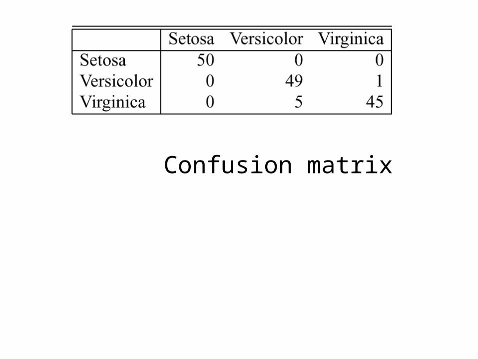
Confusion matrix

Algorithm for Decision Tree Induction
• Basic algorithm (a greedy algorithm)– Tree is constructed in a top-down recursive divide-and-
conquer manner– At start, all the training examples are at the root– Attributes are categorical (if continuous-valued, they are
discretized in advance)– Examples are partitioned recursively based on selected
attributes– Test attributes are selected on the basis of a heuristic or
statistical measure (e.g., information gain)
• Conditions for stopping partitioning– All samples for a given node belong to the same class– There are no remaining attributes for further partitioning –
majority voting is employed for classifying the leaf– There are no samples left

Information Gain (ID3/C4.5)
• Select the attribute with the highest information gain
• Assume there are two classes, P and N
– Let the set of examples S contain p elements of class P and n elements of class N
– The amount of information, needed to decide if an arbitrary example in S belongs to P or N is defined as np
nnpn
npp
npp
npI
22 loglog),(
e.g. I(0.5,0.5)=1; I(0.9,0.1)=0.47; I(0.99,0.01)=0.08;

Information Gain in Decision Tree
Induction• Assume that using attribute A a set S will
be partitioned into sets {S1, S2 , …, Sv}
– If Si contains pi examples of P and ni examples
of N, the entropy, or the expected information needed to classify objects in all subtrees Si is
• The encoding information that would be gained by branching on A
1),()(
iii
ii npInp
npAE
)(),()( AEnpIAGain

Attribute Selection by Information Gain
Computation Class P:
buys_computer = “yes”
Class N: buys_computer = “no”
I(p, n) = I(9, 5) =0.940
Compute the entropy for age:
Hence
Similarly
age pi ni I(pi, ni)<=30 2 3 0.97130…40 4 0 0>40 3 2 0.971
694.0)2,3(14
5
)0,4(14
4)3,2(
14
5)(
I
IIageE
048.0)_(
151.0)(
029.0)(
ratingcreditGain
studentGain
incomeGain
246.0
)(),()(
ageEnpIageGain

Gini Index (IBM IntelligentMiner)
• If a data set T contains examples from n classes, gini index, gini(T) is defined as
where pj is the relative frequency of class j in T.• If a data set T is split into two subsets T1 and T2
with sizes N1 and N2 respectively, the gini index of the split data contains examples from n classes, the gini index gini(T) is defined as
• The attribute provides the smallest ginisplit(T) is chosen to split the node
n
jp jTgini
1
21)(
)()()( 22
11 Tgini
NN
TginiNNTginisplit

Avoid Overfitting in Classification
• The generated tree may overfit the training data – Too many branches, some may reflect anomalies
due to noise or outliers– Result is in poor accuracy for unseen samples
• Two approaches to avoid overfitting – Prepruning: Halt tree construction early—do not
split a node if this would result in the goodness measure falling below a threshold• Difficult to choose an appropriate threshold
– Postpruning: Remove branches from a “fully grown” tree—get a sequence of progressively pruned trees• Use a set of data different from the training data
to decide which is the “best pruned tree”

Approaches to Determine the Final Tree Size
• Separate training (2/3) and testing (1/3) sets
• Use cross validation, e.g., 10-fold cross validation
• Use minimum description length (MDL) principle:
– halting growth of the tree when the encoding is minimized

Nearest Neighbor Methods
•k-NN assigns an unknown object to the most common class of its k nearest neighbors
•Choice of k? (bias-variance tradeoff again)
•Choice of metric?
•Need all the training to be present to classify a new point (“lazy methods”)
•Surprisingly strong asymptotic results (e.g. no decision rule is more than twice as accurate as 1-NN)

Flexible Metric NN Classification

Naïve Bayes ClassificationRecall: p(ck |x) p(x| ck)p(ck)
Now suppose:
Then:
Equivalently:
C
x1 x2 xp…
p
jkjkk cxpcpxcp
1
)|()()|(
)|(
)|(
)(
)(log
)|(
)|(log
kj
kj
k
k
k
k
cxp
cxp
cp
cp
xcp
xcp
“weights of evidence”

Evidence Balance Sheet

Naïve Bayes (cont.)
•Despite the crude conditional independence
assumption, works well in practice (see Friedman,
1997 for a partial explanation)
•Can be further enhanced with boosting, bagging,
model averaging, etc.
•Can relax the conditional independence
assumptions in myriad ways (“Bayesian
networks”)

Dietterich (1999)
Analysis of 33 UCI datasets


