CLASSIFICATION OF ALTERNATING KNOTS WITH TUNNEL NUMBER ONE MARC LACKENBY 1. Introduction An alternating diagram encodes a lot of information about a knot. For ex- ample, if an alternating knot is composite, this is evident from the diagram [10]. Also, its genus ([3], [12]) and its crossing number ([7], [13], [17]) can be read off directly. In this paper, we apply this principle to alternating knots with tunnel number one. Recall that a knot K has tunnel number one if it has an unknotting tunnel, which is defined to be an arc t properly embedded in the knot exterior such that S 3 - int(N (K ∪ t)) is a handlebody. It is in general a very difficult problem to determine whether a given knot has tunnel number one, and if it has, to determine all its unknotting tunnels. In this paper, we give a complete clas- sification of alternating knots with tunnel number one, and all their unknotting tunnels, up to an ambient isotopy of the knot exterior. Theorem 1. Let D be a reduced alternating diagram for a knot K. Then K has tunnel number one with an unknotting tunnel t, if and only if D (or its reflection) and an unknotting tunnel isotopic to t are as shown in Figure 1. Thus the alternating knots with tunnel number one are precisely the two-bridge knots and the Montesinos knots (e; p/q, ±1/2,p ′ /q ′ ) where q and q ′ are odd. Figure 1. 1
Transcript
CLASSIFICATION OF ALTERNATING KNOTSWITH TUNNEL NUMBER ONE
MARC LACKENBY
1. Introduction
An alternating diagram encodes a lot of information about a knot. For ex-
ample, if an alternating knot is composite, this is evident from the diagram [10].
Also, its genus ([3], [12]) and its crossing number ([7], [13], [17]) can be read off
directly. In this paper, we apply this principle to alternating knots with tunnel
number one. Recall that a knot K has tunnel number one if it has an unknotting
tunnel, which is defined to be an arc t properly embedded in the knot exterior
such that S3 − int(N (K ∪ t)) is a handlebody. It is in general a very difficult
problem to determine whether a given knot has tunnel number one, and if it has,
to determine all its unknotting tunnels. In this paper, we give a complete clas-
sification of alternating knots with tunnel number one, and all their unknotting
tunnels, up to an ambient isotopy of the knot exterior.
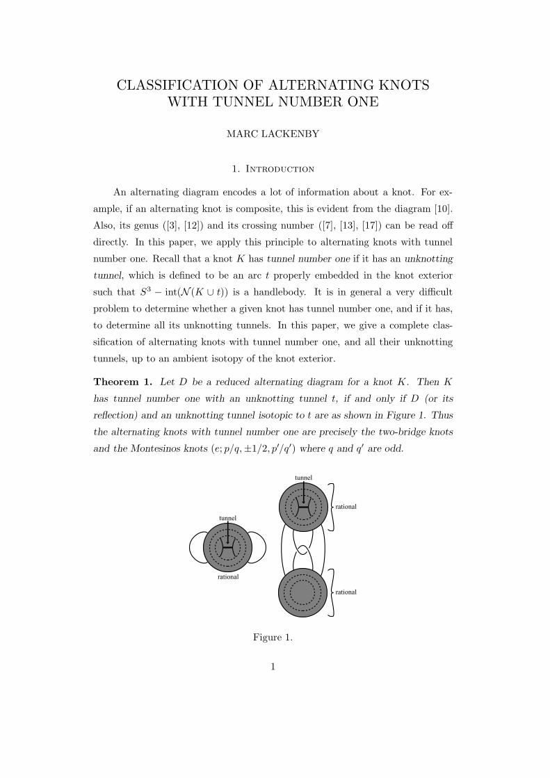
Theorem 1. Let D be a reduced alternating diagram for a knot K. Then K
has tunnel number one with an unknotting tunnel t, if and only if D (or its
reflection) and an unknotting tunnel isotopic to t are as shown in Figure 1. Thus
the alternating knots with tunnel number one are precisely the two-bridge knots
and the Montesinos knots (e; p/q,±1/2, p′/q′) where q and q′ are odd.
rational
rational
tunnel
tunnel
rational
Figure 1.
1
For an explanation of the Montesinos knot terminology, see [1]. The grey
discs in Figure 1 denote alternating diagrams of rational tangles with no nugatory
crossings. It is proved in [18] (see the comments after Corollary 3.2 of [18]) that
such a diagram is constructed by starting with a diagram of a 2-string tangle
containing no crossings and then surrounding this diagram by annular diagrams,
each annulus containing four arcs joining distinct boundary components, and each
annular diagram having a single crossing. (See Figure 2.) The boundaries of these
annuli are denoted schematically by dashed circles within the grey disc. Of course,
the signs of these crossings are chosen so that the resulting diagram is alternating.
Figure 2.
Theorem 1 settles a conjecture of Sakuma, who proposed that, when D is a
reduced alternating diagram of a tunnel number one knot K, then some unknotting
tunnel is a vertical arc at some crossing of D. For, the tunnels in Figure 1 can
clearly be ambient isotoped to be vertical at some crossing, unless the rational
tangle containing the tunnel has no crossings. But, in this case, the diagram can
be decomposed as in the left of Figure 1. In particular, the knot is a 2-bridge
knot. Hence the knot has a vertical unknotting tunnel.
A given alternating diagram D may sometimes be decomposed into the tangle
systems shown in Figure 1 in several distinct ways. Hence, the knot may have
several unknotting tunnels. For example, from Theorem 1, it is not hard to deduce
Kobayashi’s result [8], classifying all unknotting tunnels for a 2-bridge knot into
at most six isotopy classes.
We now explain why the knots in Figure 1 have tunnel number one. In the
left-hand diagram of Figure 1, contract the tunnel to a point, resulting in a graph
2
G. It is clear that, by an ambient isotopy of G, we may undo the crossings
starting with the innermost annulus and working out. Hence, the exterior of G is
a handlebody, as required.
tunnel
SWNW NE
SE
rational
Figure 3.
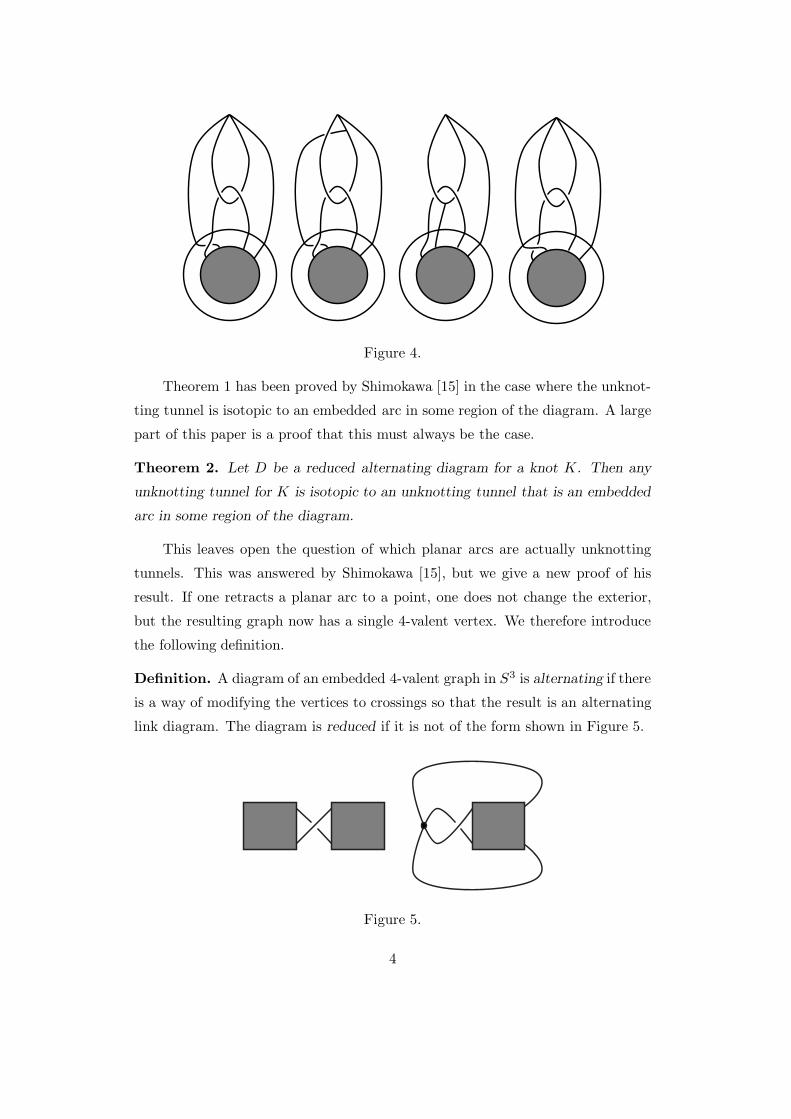
We may perform a similar procedure in the right-hand diagram of Figure 1,
resulting in Figure 3. Pick the crossing in the outermost annulus of the lower
rational tangle. If it connects the strings emanating from points SW and SE, we
may remove it. If it connects the strings emanating from NW and NE, we may
flype the rational tangle so that instead the crossing lies between SW and SE, and
then remove the crossing. If the crossing lies between points NW and SW (or NE
and SE) we may slide the graph as shown in Figure 4 without altering the exterior,
to change the crossing. This procedure does not alter the way that the two strings
of the tangle join the four boundary points. If the original diagram had more than
one crossing, then we consider the possibilities for the next annulus in the inwards
direction. By flyping if necessary, we may assume that its crossing joins SW and
SE, or SW and NW. In both these cases, the tangle has an alternating diagram
with fewer crossings. Hence, inductively, we reduce to the case where the original
tangle has at most one crossing. Since K is a knot, rather than a link, the strings
of the tangle run from NW to either SW or SE, and from NE to either SE or SW.
So, it is clear that the exterior of this graph is a handlebody.
3
Figure 4.
Theorem 1 has been proved by Shimokawa [15] in the case where the unknot-
ting tunnel is isotopic to an embedded arc in some region of the diagram. A large
part of this paper is a proof that this must always be the case.
Theorem 2. Let D be a reduced alternating diagram for a knot K. Then any
unknotting tunnel for K is isotopic to an unknotting tunnel that is an embedded
arc in some region of the diagram.
This leaves open the question of which planar arcs are actually unknotting
tunnels. This was answered by Shimokawa [15], but we give a new proof of his
result. If one retracts a planar arc to a point, one does not change the exterior,
but the resulting graph now has a single 4-valent vertex. We therefore introduce
the following definition.
Definition. A diagram of an embedded 4-valent graph in S3 is alternating if there
is a way of modifying the vertices to crossings so that the result is an alternating
link diagram. The diagram is reduced if it is not of the form shown in Figure 5.
Figure 5.
4
Morally, one perhaps should also consider a diagram as in Figure 6, where
each grey box contains at least one crossing, as not reduced. However, we will not
adopt this convention in this paper.
Figure 6.
We prove the following result which can be used to determine whether the
planar arc is an unknotting tunnel.
Theorem 3. Let D be a reduced alternating diagram of a graph G with a single
vertex. Then the exterior of G is a handlebody if and only if D is one of the
diagrams shown in Figure 7.
rational rational
Figure 7.
The dotted arcs in a grey disc denote the way that the strings of the tangle join
the four points on the boundary. Note that the middle and right-hand alternating
graphs in Figure 7 are ambient isotopic to that shown in Figure 3.
Theorem 1 is a straightforward corollary of Theorems 2 and 3. Given a
reduced alternating diagram D of a knot K with an unknotting tunnel t, we use
Theorem 2 to establish that t is isotopic to a planar arc. Contract this tunnel to a
point to form a graph G with an alternating diagram. Alter this diagram until it
5
is reduced, by removing crossings adjacent to the vertex. Theorem 3 implies that
it is of the form shown in Figure 7. Hence, D and the unknotting tunnel are as
shown in Figure 1. This proves Theorem 1.
The proof of Theorems 2 and 3 is a largely amalgamation of ideas by Ru-
binstein and Menasco. We now give a brief outline of the main arguments. It
is a well-known fact that an unknotting tunnel for a knot is determined by its
associated Heegaard surface, up to an ambient isotopy of the knot exterior. This
follows from the fact that, in a compression body C with ∂−C a torus and ∂+C
a genus two surface, ∂C has a unique non-separating compression disc up to am-
bient isotopy. Hence, we will focus on the Heegaard surface. Rubinstein showed
that, given any triangulation of a compact orientable irreducible 3-manifold M , a
strongly irreducible Heegaard surface for M can be ambient isotoped into almost
normal form [14]. An alternating knot complement inherits an ideal polyhedral
structure from its diagram [9]. We therefore in §2 develop a notion of almost
normal surfaces in such an ideal polyhedral decomposition of a 3-manifold. A
genus two Heegaard surface F for a non-trivial knot must be strongly irreducible,
and so can be ambient isotoped into almost normal form. Once in this form, F
intersects the plane of the diagram in a way rather similar to the surfaces studied
by Menasco [10]. In §3, we recall Menasco’s techniques.
It would seem logical to prove Theorem 2 before Theorem 3, but in fact the
latter result is necessary in the proof of the former. Therefore in §4, we prove
Theorem 3. The hypothesis that the graph’s exterior is a handlebody is used to
establish the existence of a compressing disc in normal form. This is then used to
show that G must be as described in the theorem.
In §5, we adapt Menasco’s arguments to restrict the possibilities for the Hee-
gaard surface F . We show that F is obtained from a standardly embedded 4-times
punctured sphere by attaching tubes that run along the knot. The sphere divides
the diagram into two tangles. We analyse the possibilities for these tangles, using
Theorem 3, and prove that the unknotting tunnel is isotopic to a planar arc in
one of them. This will prove Theorem 2 and hence Theorem 1.
6
2. Heegaard surfaces in ideal polyhedral decompositions
A reduced alternating diagram of knot determines an ideal polyhedral decom-
position of the knot complement. Hence, in this section, we develop an almost
normal surface theory for ideal polyhedral decompositions of 3-manifolds and es-
tablish that, under certain conditions, a strongly irreducible Heegaard surface can
be ambient isotoped into almost normal form.
Definition. A polyhedron is a 3-ball with a non-empty connected graph in its
boundary, the graph having no edge loops. An ideal polyhedron is a polyhedron
with its vertices removed. An ideal polyhedral decomposition of a 3-manifold M
is a way of constructing M − ∂M as a union of ideal polyhedra with their faces
identified in pairs.
Note that polyhedra cannot necessarily be realised geometrically in Euclidean
space with straight edges and faces. In particular, it is possible for a face in a
polyhedron to have only two edges in its boundary. Such faces are known as
bigons.
There is a reasonably well-established theory of normal surfaces in ideal poly-
hedra. Associated with an ideal polyhedral decomposition of a 3-manifold M ,
there is a dual handle decomposition of M , where i-handles (0 ≤ i ≤ 2) arise from
(3 − i)-cells in the ideal polyhedra. In [6], Jaco and Oertel gave a definition of
a closed normal surface in such a handle decomposition. Here we give the dual
version.
Definition. A disc properly embedded in an ideal polyhedron P is normal if
• it is in general position with respect to the boundary graph of P ,
• it intersects each edge of P at most once, and
• its boundary does not lie wholly in some face of P .
A closed properly embedded surface in a 3-manifold M is in normal form with
respect to an ideal polyhedral decomposition of M if it intersects each ideal poly-
hedron in a (possibly empty) collection of normal discs.
Note that a normal surface intersects each face in normal arcs, which means
that each arc is not parallel to a sub-arc of an edge.
7
There is also notion of normality for properly embedded surfaces with non-
empty boundary. We will come to this at the end of §3.
The following is an elementary fact about normal surfaces. The proof is an
easy generalisation of the case where each polyhedron is a tetrahedron, which can
be found in [19].
Lemma 4. Fix an ideal polyhedral decomposition of a 3-manifold in which each
face is a triangle or a bigon. Then a closed normal surface is incompressible in the
complement of the 1-skeleton.
Therefore, given any ideal polyhedral decomposition of a 3-manifold, we will
always subdivide its faces into bigons and triangles, by possibly introducing new
edges, but adding no vertices.
It is a well-known result [6] that any closed properly embedded incompress-
ible surface with no 2-sphere components in a compact orientable irreducible 3-
manifold M can be ambient isotoped into normal form with respect to some fixed
triangulation. Stocking [16], building on ideas of Rubinstein [14] and Thompson
[19], proved that any strongly irreducible Heegaard surface in M can be ambient
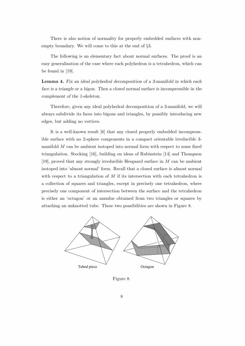
isotoped into ‘almost normal’ form. Recall that a closed surface is almost normal
with respect to a triangulation of M if its intersection with each tetrahedron is
a collection of squares and triangles, except in precisely one tetrahedron, where
precisely one component of intersection between the surface and the tetrahedron
is either an ‘octagon’ or an annulus obtained from two triangles or squares by
attaching an unknotted tube. These two possibilities are shown in Figure 8.
Tubed piece Octagon
Figure 8.
8
Stocking’s result holds true even when M has non-empty boundary: in this
case, we consider the usual definition [2] of a Heegaard splitting for M as a de-
composition into compression bodies. Recall that a compression body C is a con-
nected compact orientable 3-manifold that is either a handlebody or is obtained
from S × [0, 1], where S a closed (possibly disconnected) surface, by attaching
1-handles to S × {1}. Then we let ∂−C be S × {0}, or the empty set when C is
a handlebody, and we let ∂+C = ∂C − ∂−C. A Heegaard splitting for a compact
orientable 3-manifold M is a decomposition of M into two compression bodies
glued along their positive boundaries.
One feature of octagonal and tubed pieces is that the resulting almost normal
surface F has an edge compression disc, namely a disc D embedded in a tetrahe-
dron ∆ such that D ∩ ∂∆ lies in ∂D and is a sub-arc of an edge, and D ∩F is the
remainder of ∂D. There is one aspect of polyhedral decompositions that makes
them a little more complicated than triangulations. If a disc properly embedded
in a tetrahedron intersects each face in a collection of normal arcs and has an
edge compression disc on one side, then it has an edge compression disc on the
other side also. This need not be true in more general polyhedra. Therefore we
introduce the following definition.
Definition. Let F be a closed two-sided surface properly embedded in a compact
orientable 3-manifold with an ideal polyhedral decomposition. Then F is normal
to one side if
(i) its intersection with any face is a collection of normal arcs,
(ii) its intersection with any ideal polyhedron is a collection of discs, and
(iii) all edge compression discs for any of these discs emanate from the same side
of F .
Note that a surface that is normal to one side may in fact be a normal sur-
face. However, we will often refer to ‘the’ normal side of the surface, with the
understanding that if the surface is normal, then this means either side. We
now introduce a generalisation of almost normality to surfaces in ideal polyhedral
decompositions.
9
Definition. Let P be an ideal polyhedron in which each face is a triangle or
bigon. An almost normal disc in P is a properly embedded disc D having the
following properties:
(i) its intersection with each face is a collection of normal arcs,
(ii) in each component of cl(P − D) there is an edge compression disc, and
(iii) any two edge compression discs, one on each side of D, must intersect in the
interior of P .
Let M be a compact orientable 3-manifold with an ideal polyhedral decomposition
in which each face is a triangle or bigon. A closed properly embedded surface in
M is almost normal if either
(a) its intersection with each ideal polyhedron is a collection of normal discs,
except in precisely one ideal polyhedron where it has precisely one almost
normal disc, together possibly with some normal discs, or
(b) it is obtained from a normal surface by attaching a tube that lies in a single
ideal polyhedron, that runs parallel to an edge and that joins distinct normal
discs.
An example of an almost normal disc is shown in Figure 9.
Figure 9.
10
Theorem 5. Let F be a strongly irreducible Heegaard surface for a compact
orientable irreducible 3-manifold M . Fix an ideal polyhedral decomposition of M
in which each face is a bigon or triangle. Suppose that M contains no 2-spheres
that are normal to one side. Then there is an ambient isotopy taking F into almost
normal form.
The proof of this theorem follows Stocking’s argument [16] very closely. We
therefore will only sketch the main outline and will refer the reader to [16] for
further details.
The hypothesis that M contains no 2-spheres that are normal to one side
is an unfortunate one. Although this theorem is sufficient for our purposes, it is
possible that this assumption can be dropped, with some substantial work. Normal
2-spheres caused significant complications in Stocking’s proof, and the possibility
of 2-spheres that are normal to only one side causes even more difficulties.
We will need the following lemma, which is a translation of Lemma 1 in [16] to
the polyhedral setting. However, the proof in [16] involves a case-by-case analysis
that is not suitable here. We therefore give an alternative proof.
Lemma 6. Let S be a closed separating properly embedded surface in a compact
orientable irreducible 3-manifold M with an ideal polyhedral decomposition in
which each face is a triangle or bigon. Suppose that S is almost normal or normal
to one side. Suppose also that S is incompressible into one component I of M −
int(N (S)), and that S has an edge compression in I . Then S is ambient isotopic
to a surface in I , each component of which is either normal or a 2-sphere lying
entirely in a single ideal polyhedron.
Proof. We will perform a sequence of isotopies that move S into I . At each stage,
we will denote the new surface by S and the new component of M−int(N (S)) into
which S is incompressible by I . We are assuming that S has an edge compression
disc in I . This specifies an ambient isotopy that reduces the weight of surface.
Perform this ambient isotopy into I . The result is a surface that need not be
normal, but which has the following properties:
(i) for any component B of intersection between I and a polyhedron, the inter-
section between B and any face has at most one component;
11
(ii) if an arc of intersection between S and some face has endpoints on the same
edge, and D is the subdisc of the face that it separates off, then the interior
of D is disjoint from S and is a subset of I ;
(iii) if C is a simple closed curve of intersection between S and some face, and D
is the subdisc of the face that it separates off, then the interior of D is disjoint
from S and is a subset of I ;
(iv) any component of intersection between S and a polyhedron P is incompress-
ible in the M − I direction;
(v) for any component B of intersection between I and a polyhedron P , ∂B ∩ P
is boundary-parallel in P .
Note that (i) need not apply to S before the isotopy. But it does afterwards.
Otherwise, we may find an edge compression disc for the original S in M − I with
the property that it and the edge compression disc in I do not intersect away from
the 2-skeleton of M . This contradicts the assumption that S is almost normal or
normal to one side.
Suppose that in some polyhedron P , S ∩ P is not a collection of discs and
2-spheres. Then S ∩P has a compression disc D in P . This disc lies in I , by (iv).
Hence, ∂D bounds a disc D′ in S. Ambient isotope D′ onto D.
Note that if S intersects some face in a simple closed curve, but S ∩ P does
not admit a compression in any polyhedron P , then this is the only intersection
between this component of S and the 2-skeleton. By (iii), this 2-sphere bounds a
3-ball in I , and we may ambient isotope it into a single ideal polyhedron.
Suppose that, for some polyhedron P and some component D of S ∩ P , D
intersects some edge e more than once. We may assume that there are two adjacent
points of intersection between D and e. Hence, there is an edge compression disc.
This edge compression disc must lie in I , otherwise we contradict (i) or (ii). Hence,
we use this to perform an isotopy into I , reducing the weight of the surface.
After each of these isotopies, properties (i) - (v) still hold. Eventually, this
process must terminate in the required surface.
Corollary 7. If M contains no normal 2-spheres, then it contains no almost
12
normal 2-spheres.
Proof. Let S be an almost normal 2-sphere, and let M1 and M2 be the two
components of M − int(N (S)). By Lemma 6, we may ambient isotope S into each
Mi until it is normal or disjoint from the 2-skeleton. The former case is impossible,
by hypothesis. Thus, S must bound a 3-ball in both sides. Therefore, M is the
3-sphere, which is closed, but closed 3-manifolds do not have an ideal polyhedral
decomposition.
We will prove Theorem 5 by induction. At each stage, we will consider a
connected compact 3-manifold Mi embedded in M such that
(i) ∂Mi is normal in M , and
(ii) F lies in Mi and is a Heegaard surface for Mi.
Initially, M1 = M . Note that Mi inherits an ideal polyhedral decomposition from
that of M , by taking the intersection between Mi and the ideal polyhedra of M ,
and then removing ∂Mi. The hypothesis that ∂Mi is normal in M guarantees
that surfaces that are normal, normal to one side or almost normal in Mi have
the same property in M .
At each stage of the induction, we either deliver the Heegaard surface F in
almost normal form, or we construct a new embedded 3-manifold Mi+1 contained
in Mi, that satisfies (i) and (ii) above. The boundary of Mi+1 will not be parallel in
the ideal polyhedral decomposition to that of Mi. A straightforward modification
of the standard argument due to Kneser gives that there is an upper bound on the
number of such surfaces in M [5]. So, we eventually obtain F in almost normal
form. We now give the main steps of the argument.
The Heegaard splitting for Mi determines a singular foliation, as follows.
In the case where a compression body C is a handlebody, the singular set in
C is a graph onto which C collapses; otherwise it is the cores of the 1-handles.
The complement of the singular set and ∂−C is given a product foliation F ×
(0, 1). A small isotopy guarantees that the 1-skeleton ∆1 of the ideal polyhedral
decomposition is disjoint from the singular set. We then place ∆1 in thin position
with respect to F × (0, 1). The following proposition is the key step.
Proposition 8. There is a non-singular leaf F of the foliation, which either is
13
almost normal or can be compressed on one side in the complement of the 1-
skeleton to a (possibly disconnected) almost normal surface F . In the latter case,
the incompressible side of F has an edge compression disc.
Proof. There are two cases to consider: when there is a thick region and when
there is not. Consider first the case where there is no thick region. Then we take
F to be a leaf in the foliation having the maximal number number of points of
intersection with ∆1. This is obtained from ∂−C for one of the compression bodies
C, by attaching tubes, which are the boundaries of small regular neighbourhoods
of the singular set. The argument of Lemma 4 in [16] gives that, after possibly
compressing some of these tubes to one side, we obtain an almost normal surface
that contains a tubed component. If any compressions were used, the resulting
surface is incompressible to one side, as F is strongly irreducible [2]. The edge
compression disc for the tube lies on this side. (Essentially, Lemma 4 in [16] barely
uses that the hypothesis that M is triangulated; instead it is an analysis of how
the tubes lie in the ideal polyhedral decomposition.)
Consider now the case where there is a thick region. Applying the proof of
Claim 4.4 in [19], we can find a leaf F of the foliation in the thick region, which
intersects each face in a collection of normal arcs and simple closed curves. It has
an upper and a lower disc. The assumption that this is thin position guarantees
that any two such discs must intersect at other than their endpoints. We compress
F , if necessary, to a (possibly disconnected) surface F which intersects each face
only in normal arcs, and which intersects each ideal polyhedron in discs.
We claim that F is normal to one side or almost normal. If F has edge
compression discs on at most one side, it is normal to one side. If it has edge
compression discs on both sides, they must lie in the same polyhedron, otherwise
we contradict thin position. By the argument of Claims 4.1 to 4.3 in [19], at
most one disc of F in this polyhedron can be non-normal, and it must be almost
normal. We indicate briefly how this argument runs. Any edge compression
disc for any disc of F can be isotoped so that its interior is disjoint from F .
For, otherwise, F (and hence F ) has a pair of nested upper and lower discs,
contradicting thin position. Thus, if F contains two non-normal discs, we may
find disjoint edge compression discs, one emanating from each side of F . These
form disjoint upper and lower discs for F , which is a contradiction. Similarly, any
14
two edge compression discs for a disc of F , one on each side of F , must intersect
away from their boundaries. This proves the claim.
Now, F is obtained from F by attaching tubes. We claim that they are not
nested, and that their meridian discs all lie on the same side of F . For if they are
nested, then we may pick a tube T , with at least one tube running through it,
but such that all tubes T1, . . . Tn running through T are innermost. Let Di be a
meridian disc for Ti, and let D be a meridian disc for T . If Di is not a compression
disc for F , then ∂Di bounds a disc in F . If this disc contains any tubes, consider
the simple closed curves forming the boundaries of their meridian discs. Pass to
an innermost such curve. This bounds a disc in F which forms part of a 2-sphere
component of F . But we have made the assumption that M contains no 2-spheres
that are normal to one side. By Corollary 7, M also contains no almost normal
2-spheres. Thus, no component of F is a 2-sphere. Thus, each Di is a compression
disc for F . So, when we compress F along these discs, the resulting surface F ′ is
incompressible on the side containing D, as F is strongly irreducible. Therefore,
∂D bounds a disc in F ′. Again, this implies that F contains a 2-sphere component,
which is a contradiction. Therefore, the tubes of F are not nested. Their meridian
discs are all essential. Since F is strongly irreducible, they all lie on the same side
of F . This proves the claim.
We claim that F is almost normal, giving the required surface. Suppose that,
on the contrary, F is normal to one side. Now, F has both upper and lower discs.
By the argument in Claim 11 of [16], we may assume that they are disjoint from
the interiors of the tubes. Thus, on the side of F to which the tubes are not
attached, there must be an edge compression disc, making that side non-normal.
So, the tubes are attached to the normal side of F . Then, since the tubes of F
are not nested and all emanate from the same normal side, we may apply by the
argument of Lemma 4 in [16] to deduce that there is an edge compression disc for
F that runs over one tube exactly once. This and the edge compression disc on
the non-normal side of F form upper and lower discs for F that intersect away
from ∆1, which is a contradiction.
If F is almost normal, Theorem 5 is proved. If not, then by Proposition 8, it
compresses on one side to an almost normal surface F . Let I be the incompressible
side of F . The tubes of F are all attached to this side, and hence lie in I . Apply
15
Lemma 6 to ambient isotope F into I to a normal surface. Let Mi+1 be the copy
of I after the ambient isotopy. This has the required properties. Hence the proof
of Theorem 5 is complete.
3. Polyhedral decompositions of alternating knot complements
It is well known that a reduced diagram of a knot induces a decomposition
of the knot complement into two ideal polyhedra. The construction is due to
Menasco [9]. We recall the main details now. Suppose we are given a reduced
knot diagram D lying in a 2-sphere. We embed this 2-sphere into S3. The knot
lies in this 2-sphere, except near each crossing, where it skirts above and below the
diagram as two semi-circular arcs (see Figure 10). These arcs lie on the boundary
of a 2-sphere ‘bubble’ that encloses each crossing. The 2-sphere containing the
diagram decomposes each bubble into two discs, an upper and lower hemisphere.
The upper (respectively, lower) hemispheres together with the remainder of the
diagram 2-sphere is a 2-sphere denoted S2+ (respectively, S2
−). We will use S2
±to
denote S2− or S2
+.
Bubble
Figure 10.
At each crossing there is a vertical arc properly embedded in the knot com-
plement. These arcs form the edges of the ideal polyhedral decomposition. There
is one face for each region of the diagram. (See Figure 11.) The complement of
the edges and faces is two open 3-balls, one above the diagram, one below. These
open balls are the interior of the two ideal polyhedra.
A closed normal or almost normal surface F in this ideal polyhedral de-
composition can be visualised in quite a straightforward way. At each point of
intersection between F and an edge, we insert at a saddle in the relevant bubble
16
(see Figure 12). The intersection between F and the faces of the polyhedra is a
collection of arcs which lie in the regions of the diagram. The condition that F
is normal (or almost normal) and that the diagram is reduced guarantees that no
arc has endpoints in the same crossing.
Edge
Face
Figure 11.
Figure 12.
We will need to consider surfaces that are more general than normal surfaces.
Let F be a surface properly embedded in the knot complement, such that any
boundary component of F is meridional. We say that F is standard if it intersects
each bubble in a collection of saddles, intersects each face in a collection of arcs and
intersects the two truncated polyhedra in a collection of discs. Also, the boundary
C of each such disc must satisfy the following conditions:
(i) no arc of intersection between C and a face has endpoints lying in the same
crossing;
(ii) if C intersects the knot, it does so transversely away from the bubbles;
(iii) C intersects the knot projection in more than two points.
A central part of Menasco’s techniques [10] is to analyse how a normal sur-
17
face F lies in an alternating knot complement. Under many circumstances, he
established the existence of a meridional compression disc which is defined to be
an embedded disc R such that R ∩ F = ∂R and R ∩ K is a single point in the
interior of R. The meridional compression disc that Menasco constructs is dia-
grammatic which means that its intersection with the bubbles is a single disc in
a single bubble, and the remainder of the disc is disjoint from the plane of the
diagram.
We say that a 2-sphere is trivial if it is disjoint from the bubbles and it
intersects the plane of the diagram in a single simple closed curve.
The following is a generalisation of Menasco’s results to standard surfaces.
Lemma 9. Let D be a prime alternating diagram of a knot K, and let F be
a standard surface properly embedded in the knot exterior with at most two
meridional boundary components. Then either F is a trivial twice-punctured 2-
sphere, or it admits a diagrammatic meridional compression.
Proof. We claim that we can find a simple closed C of F ∩ S2+ that intersects
some bubble in at least two arcs, where two of these arcs are part of the same
saddle and have no arc of F ∩S2+ between them. We can then find a simple closed
curve in F that runs from C across the saddle back to C and then over the disc
that C bounds above the diagram. This curve bounds the required diagrammatic
meridional compression disc.
If there is only one curve of F ∩S2+, then it is either disjoint from the bubbles,
in which case F is a trivial twice-punctured 2-sphere, or it intersects some bubble as
claimed. Thus, we may assume that there are at least two such curves. Consider
an innermost one, C, bounding a disc I containing no other curves of F ∩ S2+.
By choosing this curve suitably, we can ensure that C has at most one point of
intersection with K, since F has at most two boundary components.
Each time that C runs over a bubble, the crossing either lies in the inward
direction or outward direction from C. Note, however, that just because a crossing
lies in the inward direction from C, this does not guarantee that the crossing itself
lies in I , since C may return to the crossing several times. The hypothesis that
the diagram is alternating ensures that, as one runs along C, one meets crossings
18
alternately on the inward direction and outward direction of C.
Consider the arc components of intersection between I and the knot projec-
tion, ignoring the components containing crossings. Suppose first that there are
at least two such arcs. Let α be an outermost such arc in I , separating off a disc
E. By choosing α appropriately, we can ensure that E ∩ C is disjoint from K. It
therefore runs from a bubble back to the same bubble. It meets this bubble once
in the inwards direction and once in the outwards direction. Hence, by property
(i) in the definition of a standard surface, it runs over at least one other bubble
in the inwards direction. Consider the curve of F ∩ S2+ on the other side of this
crossing, connected via the saddle at the bubble. This must again be part of C,
by the assumption that C is innermost. Hence, we have the found the required
intersection with C and a bubble.
Suppose now that there is precisely one arc α of intersection between I and
the knot projection. If C∩K does not lie at an endpoint of α, the above argument
works. Suppose therefore that C ∩ K does lie at an endpoint of α. Note that C
must meet at least one other crossing, by (iii) in the definition of a standard
surface. Hence, it meets a crossing in the inwards direction, and the claim is then
proved.
Suppose now that there is no arc of intersection between I and the knot
projection. Now, C must meet at least three crossings, at least one of which lies
in the inward direction. Thus, as above, the claim is proved.
F
F FF
MeridionalcompressionK
Figure 13.
Let F be the result of F immediately after the diagrammatic meridional
compression. Then F satisfies all the conditions of a standard surface, except
possibly (iii). This may fail, since F may have one or two ‘tubes’ that run parallel
to the knot for a time before closing off with a disc that intersects the knot in a
19
single point. We now explain how to modify F by retracting these tubes, under the
assumption that the diagram is prime. Each component of the resulting surface
will be standard or a trivial 2-sphere. For, if (iii) fails for a component of F that
is not a trivial 2-sphere, then there is then an ambient isotopy which retracts this
tube, reducing the number of curves of F ∩S2+ and leaving the number of curves of
F∩S2− unchanged. Clearly, (i) and (ii) still hold, and the surface still intersects the
bubbles in saddles, the faces in arcs and the polyhedra in discs. Hence, eventually,
each component is a trivial 2-sphere or a standard surface.
Corollary 10. Let D be a prime alternating diagram of a knot K. Then
(i) the exterior of K contains no standard 2-spheres that intersect the knot in at
most two points;
(ii) any standard torus disjoint from the knot is normally parallel to ∂N (K).
Proof. Let F be a standard 2-sphere disjoint from the knot. Then by Lemma 9,
F admits a meridional compression. The result is two 2-spheres, each of which
intersects the knot once, which is impossible.
Now consider a standard 2-sphere F intersecting K in two points. We will
prove, by induction, on the number of its saddles that such a 2-sphere cannot
exist. It admits a meridional compression to two such 2-spheres. Retract the
tubes of these 2-spheres. The result, inductively, cannot be standard 2-spheres.
Hence, they must be trivial. However, if we then reconstruct F by tubing these
two trivial 2-spheres together, the result is not standard.
Finally, let F be a standard torus disjoint from the knot. Find a diagrammatic
meridional compression to a twice punctured 2-sphere. Retract its tubes. The
result cannot be standard, and hence must be trivial. Therefore, the original
torus F must have been normally parallel to ∂N (K).
A further variation that we need to consider is alternating graphs as opposed
to alternating knots. In this case, we will need to analyse surfaces with non-
meridional boundary properly embedded in the graph exterior. Again, there is a
theory of normal surfaces, following [6]. If one truncates the ideal vertices of the
ideal polyhedral decomposition, the resulting truncated polyhedra have boundary
that can be identified with S2±. A properly embedded surface is normal if it
20
intersects each bubble in a collection of saddles, intersects each face in a collection
of arcs and intersects the two truncated polyhedra in a collection of discs. Also,
the boundary C of each such disc must satisfy the following conditions:
(i) C intersects each side of each crossing in at most one arc;
(ii) C does not lie entirely in ∂N (G) ∩ S2±;
(iii) no arc of intersection between C and a face F has endpoints lying in the
same crossing, or in the same component of ∂N (G)∩ F , or in a crossing and
a component of ∂N (G) ∩ F that are adjacent;
(iv) C intersects any component of N (G) ∩ S2± in at most one arc;
(v) any such arc cannot have endpoints in the same component of N (G) ∩ F for
any face F .
4. Alternating graphs with handlebody exteriors
The main goal of this section is to prove Theorem 3 below.
Theorem 3. Let D be a reduced alternating diagram of a graph G with a single
vertex. Then the exterior of G is a handlebody if and only if D is one of the
diagrams shown in Figure 7.
We will use the following lemma at a number of points.
Lemma 11. Let D be a reduced alternating diagram of a graph G with a single
vertex, such that the exterior of G is a handlebody H . Let C be a simple closed
curve in the diagram that intersects the graph projection transversely in two points
disjoint from the crossings and the vertex. Then C bounds a disc in D that is
disjoint from the crossings and the vertex.
Proof. Suppose, on the contrary, that there is such a curve C, bounding a disc in
D that is disjoint from the vertex but contains at least one crossing. It bounds
two discs, one above the diagram, and one below. The union of these is a 2-sphere,
whose intersection with H is an annulus A. The core curve of A is homologically
non-trivial in H . Hence, A is incompressible in H . When a handlebody is cut along
a properly embedded orientable incompressible surface, the result is a disjoint
21
union of handlebodies. Hence, the 1-string tangle that C bounds must be trivial.
But this contradicts Menasco’s theorem [10], since it is reduced, alternating and
has at least one crossing.
Proof of Theorem 3. We argued in the introduction that the exteriors of the graphs
in Figure 7 are handlebodies. Hence, we need only prove the converse.
Suppose now that the exterior of G is a handlebody. Its boundary therefore
has a compression disc. Hence, by [6], it has a compression disc E in normal form.
Note that E cannot have a meridional compression disc E1. For ∂E1 would then
bound a subdisc E2 of E, and E1∪E2 would be an embedded 2-sphere intersecting
G in precisely one point, which is impossible.
Consider the intersection between E and S2− ∪S2
+. This is a graph embedded
in E. Its complimentary regions are saddles and normal discs, where the former
lie in the interior of E. If this graph fails to be connected, then pick a component
that is outermost in E. Let E ′ be the subdisc of E comprised of this component
and all faces adjacent to it. Suppose that the region of E ′ containing ∂E ′ − ∂E
lies below S2−, say. Then we will focus E ′ ∩ S2
+. This has the property that any
curve of E ′ ∩ S2+ runs over ∂N (G) at most once. Also, if E ′ ∩ S2
+ runs over a
saddle, then the curve of E ∩ S2+ on the other side of the crossing also lies in E ′.
Let N be the component of N (G)∩S2+ containing the vertex v. If N is not a
disc, then one of the components β of G−v runs from v back to v without passing
underneath any crossings. Since G is alternating, it therefore runs through at
most one over-crossing. Suppose first that β runs through no crossings. Then
the remainder of the diagram is a diagram of the other component of G − v. By
Lemma 11, this tangle has no crossings. Then, D is as in the leftmost diagram of
Figure 7. If β runs through a single crossing, then it divides the diagram into two
1-string tangles. Each tangle has no crossings by Lemma 11. Hence, the diagram
of G has a single crossing, and therefore fails to be reduced. We may therefore
assume that N is a disc. Note that ∂N runs through crossings eight times.
We perform a small ambient isotopy so that all curves of E ′ ∩S2+ are disjoint
from the vertex v of G. We can ensure that, for any curve C of E ′ ∩ S2+, the disc
of S2+ that C bounds not containing v contains at most four crossings in ∂N .
22
Pick a curve C of E ′ ∩ S2+ innermost in the diagram, where we define the
innermost direction so that the disc that C bounds does not contain v.
Consider first the case where C is disjoint from N (G). Then it runs over an
even number of crossings. As in the proof of Lemma 7, the fact that the diagram is
alternating and that C is innermost implies that E has a meridional compression
disc, which is impossible.
Thus C must run over N (G). The arc C−N (G) runs over at most one saddle.
Otherwise, we would either contradict the assumption that C is innermost or we
would find a meridional compression disc for E.
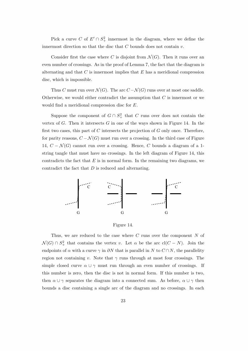
Suppose the component of G ∩ S2+ that C runs over does not contain the
vertex of G. Then it intersects G in one of the ways shown in Figure 14. In the
first two cases, this part of C intersects the projection of G only once. Therefore,
for parity reasons, C −N (G) must run over a crossing. In the third case of Figure
14, C − N (G) cannot run over a crossing. Hence, C bounds a diagram of a 1-
string tangle that must have no crossings. In the left diagram of Figure 14, this
contradicts the fact that E is in normal form. In the remaining two diagrams, we
contradict the fact that D is reduced and alternating.
G GG
C C C
Figure 14.
Thus, we are reduced to the case where C runs over the component N of
N (G) ∩ S2+ that contains the vertex v. Let α be the arc cl(C − N ). Join the
endpoints of α with a curve γ in ∂N that is parallel in N to C ∩N , the parallelity
region not containing v. Note that γ runs through at most four crossings. The
simple closed curve α ∪ γ must run through an even number of crossings. If
this number is zero, then the disc is not in normal form. If this number is two,
then α ∪ γ separates the diagram into a connected sum. As before, α ∪ γ then
bounds a disc containing a single arc of the diagram and no crossings. In each
23
case, this implies that the diagram fails to be reduced and alternating, or E fails
to be normal. Hence, α ∪ γ runs through precisely four crossings. We list all
the possibilities in Figure 15. We have not included any possibilities that would
contradict the fact that the diagram is alternating.
C not innermost
aa
a
a
a
Diagram is aconnected sum
Diagram is aconnected sum
Figure 15.
It is clear that only two of these diagrams may arise. In both cases, Figure
16 shows a way of removing the vertex and replacing it with two arcs.
a
a
Figure 16.
24
The result is a composite alternating diagram of a knot or link L. It has
no trivial loops (namely, a loop that starts and ends at the same crossing, with
interior disjoint from the crossings). Hence, L is composite by [10]. This link L
has tunnel number one, since there is an obvious unknotting tunnel t such that the
exterior of L ∪ t is homeomorphic to the exterior of G. A result of Gordon-Reid
[4] asserts that a tunnel number one knot or link can be composite only if it has
a Hopf link summand. The Hopf link has a unique reduced alternating diagram
[11]. Therefore, in the diagram of L, one of its components runs through exactly
two crossings, forming a meridian of the other component. Since G is connected,
these two components are fused together at v. Thus, a subset of D is as shown in
Figure 17. Note that this is identical to the complement of the grey discs in either
the middle or right-hand diagrams of Figure 7.
A
G
Figure 17.
We need to show that the remainder of the diagram is a rational tangle. The
strings of this tangle must join up as shown in Figure 7, since G is connected. Let
S be the 2-sphere bounding the subset of the diagram in Figure 17. This sphere
divides S3 into two 3-balls, B1 and B2, where we say that B2 is the one containing
the vertex v.
We need to show that the tangle G ∩ B1 is rational. Let A be the annulus
shown in Figure 17 properly embedded in the exterior of G. Note that there is
a homeomorphism h from S3 − int(N (G ∪ A)) to B1 − int(N (G ∩ B1)), taking
the two copies of A in ∂N (G∪A) to the two annuli cl(∂N (G∩ B1)− ∂B1). This
annulus A is incompressible in the complement of G. But the exterior H of G is
a handlebody. Hence, A admits a ∂-compression in H . The image under h of this
∂-compression disc is a disc P embedded in B1 −G. Note that P ∩∂B1 is a single
25
arc, and the remainder of ∂P runs once along one component of G ∩ B1. Hence,
P specifies a parallelity disc between this component of G∩B1 and an arc in ∂B1.
The remaining arc of G ∩ B1 lies in the complement of P , which is a 3-ball. It
must be a trivial 1-string tangle in this 3-ball. Hence, the intersection of B1 with
G is a rational tangle. This proves that G is as shown in Figure 7.
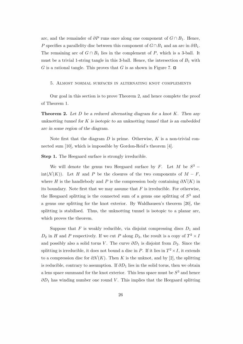
5. Almost normal surfaces in alternating knot complements
Our goal in this section is to prove Theorem 2, and hence complete the proof
of Theorem 1.
Theorem 2. Let D be a reduced alternating diagram for a knot K. Then any
unknotting tunnel for K is isotopic to an unknotting tunnel that is an embedded
arc in some region of the diagram.
Note first that the diagram D is prime. Otherwise, K is a non-trivial con-
nected sum [10], which is impossible by Gordon-Reid’s theorem [4].
Step 1. The Heegaard surface is strongly irreducible.
We will denote the genus two Heegaard surface by F . Let M be S3 −
int(N (K)). Let H and P be the closures of the two components of M − F ,
where H is the handlebody and P is the compression body containing ∂N (K) in
its boundary. Note first that we may assume that F is irreducible. For otherwise,
the Heegaard splitting is the connected sum of a genus one splitting of S3 and
a genus one splitting for the knot exterior. By Waldhausen’s theorem [20], the
splitting is stabilised. Thus, the unknotting tunnel is isotopic to a planar arc,
which proves the theorem.
Suppose that F is weakly reducible, via disjoint compressing discs D1 and
D2 in H and P respectively. If we cut P along D2, the result is a copy of T 2 × I
and possibly also a solid torus V . The curve ∂D1 is disjoint from D2. Since the
splitting is irreducible, it does not bound a disc in P . If it lies in T 2×I , it extends
to a compression disc for ∂N (K). Then K is the unknot, and by [2], the splitting
is reducible, contrary to assumption. If ∂D1 lies in the solid torus, then we obtain
a lens space summand for the knot exterior. This lens space must be S3 and hence
∂D1 has winding number one round V . This implies that the Heegaard splitting
26
is reducible, which is a contradiction. This proves that F is strongly irreducible.
Step 2. Placing F into almost normal form.
Pick some subdivision of the faces of the ideal polyhedral decomposition of
the knot complement, without introducing any vertices, so that each face is bigon
or triangle. By Corollary 10, this contains no properly embedded standard 2-
spheres. In particular, it contains no 2-spheres that are normal to one side. So,
by Theorem 5, we may ambient isotope F into almost normal form in this ideal
polyhedral decomposition.
Consider first the case where F has an almost normal tubed piece. Compress
this tube. The result is a surface that is normal to one side. By Corollary 10, it
contains no 2-sphere components. Hence, it is one or two tori. In the latter case,
one of these tori would be compressible. Each torus is standard, and hence, by
Corollary 10, is normally parallel to ∂N (K). In particular, it is incompressible.
Thus, the compressed surface is a single torus F that is normally parallel to
∂N (K). Up to isotopy, the unknotting tunnel runs from ∂N (K) through the
tube and then to ∂N (K), respecting the product structure in the tube and the
product structure on the parallelity region between ∂N (K) and F . This arc can
therefore be ambient isotoped into a face of the ideal polyhedral decomposition.
This is then an embedded arc in some region of the diagram. This proves Theorem
2 in this case.
We therefore assume now that the almost normal surface F contains no almost
normal tubed piece.
Step 3. Meridionally compressing F .
By Lemma 9, F admits a diagrammatic meridional compression to a twice-
punctured torus T . Retract the tubes of T to place it in standard form. Now
apply Lemma 9 again to find another meridional compression disc. There are
two possibilities for the resulting surface: either a 2-sphere intersecting K in four
points or a torus intersecting K in two points and a 2-sphere intersecting K twice.
We claim that the latter case cannot arise. For the twice-punctured 2-sphere
retracts to a trivial 2-sphere by Corollary 10. But, then reconstructing T , we see
that it could not have been standard. Hence, the meridional compression must
27
yield a 2-sphere S intersecting K in four points.
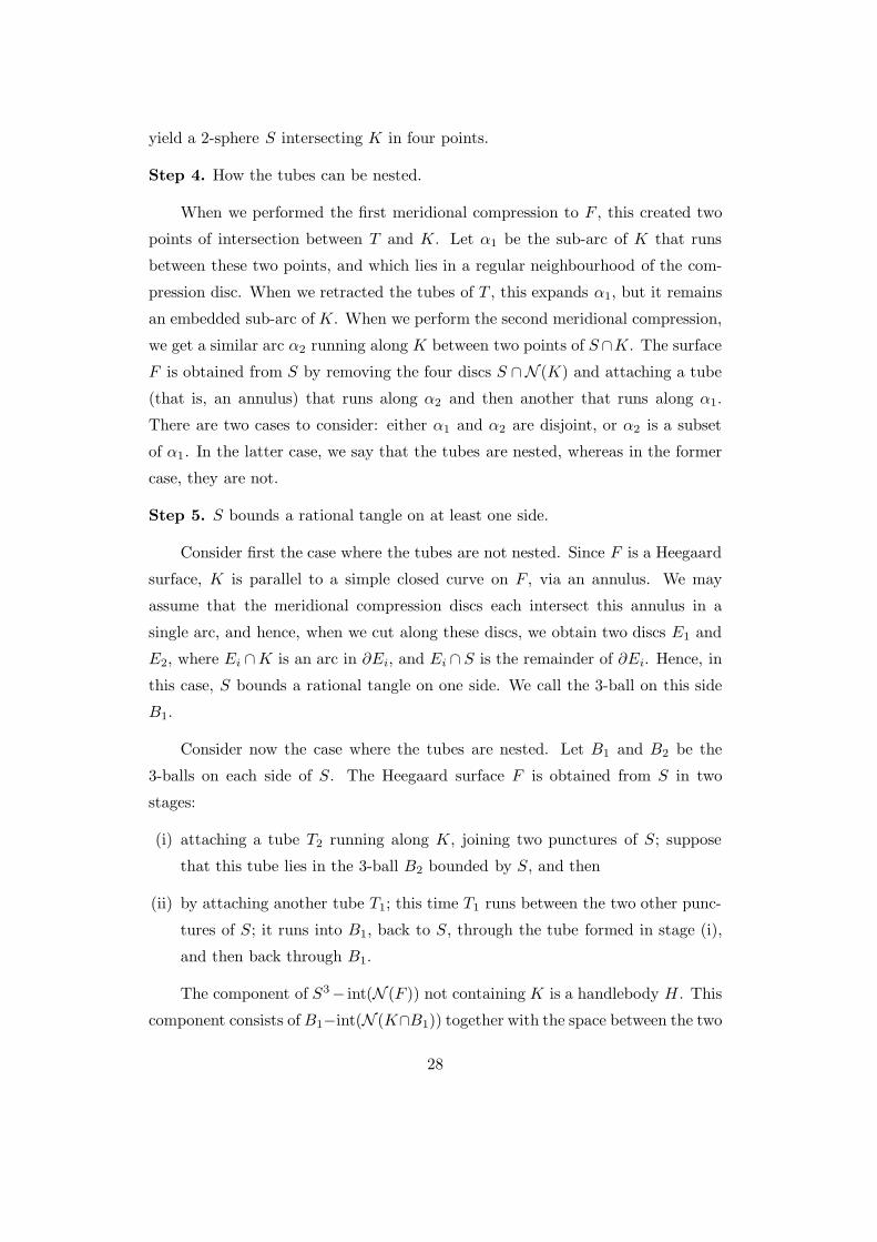
Step 4. How the tubes can be nested.
When we performed the first meridional compression to F , this created two
points of intersection between T and K. Let α1 be the sub-arc of K that runs
between these two points, and which lies in a regular neighbourhood of the com-
pression disc. When we retracted the tubes of T , this expands α1, but it remains
an embedded sub-arc of K. When we perform the second meridional compression,
we get a similar arc α2 running along K between two points of S∩K. The surface
F is obtained from S by removing the four discs S ∩N (K) and attaching a tube
(that is, an annulus) that runs along α2 and then another that runs along α1.
There are two cases to consider: either α1 and α2 are disjoint, or α2 is a subset
of α1. In the latter case, we say that the tubes are nested, whereas in the former
case, they are not.
Step 5. S bounds a rational tangle on at least one side.
Consider first the case where the tubes are not nested. Since F is a Heegaard
surface, K is parallel to a simple closed curve on F , via an annulus. We may
assume that the meridional compression discs each intersect this annulus in a
single arc, and hence, when we cut along these discs, we obtain two discs E1 and
E2, where Ei ∩K is an arc in ∂Ei, and Ei ∩ S is the remainder of ∂Ei. Hence, in
this case, S bounds a rational tangle on one side. We call the 3-ball on this side
B1.
Consider now the case where the tubes are nested. Let B1 and B2 be the
3-balls on each side of S. The Heegaard surface F is obtained from S in two
stages:
(i) attaching a tube T2 running along K, joining two punctures of S; suppose
that this tube lies in the 3-ball B2 bounded by S, and then
(ii) by attaching another tube T1; this time T1 runs between the two other punc-
tures of S; it runs into B1, back to S, through the tube formed in stage (i),
and then back through B1.
The component of S3− int(N (F )) not containing K is a handlebody H . This
component consists of B1−int(N (K∩B1)) together with the space between the two
28
tubes, which is a copy of A× I , where A is an annulus and where (A× I)∩ B1 =
A × ∂I . Then A × {1
2} is an incompressible annulus properly embedded in a
handlebody. Such an annulus must have a boundary-compression disc E. We may
assume that E intersects A × I as the product of a properly embedded essential
arc in A and either [0, 1
2] or [1
2, 1]. We may also assume that E intersects the
remainder of T1 in a single arc. By extending E− (A× (0, 1)) a little, we obtain a
disc E ′ embedded in B1, such that ∂E ′ is the union of an arc of K ∩B1 and an arc
in ∂B1. The other arc of K ∩ B1 lies in B1 − int(N (E ′)), which is a 3-ball. This
arc must also be trivial, since H− int(N (A)) is a handlebody. Hence, (B1, B1∩K)
is a rational tangle.
Step 6. The possible positions for S.
We retract the tubes of S to a standard surface. In [10], Menasco analysed
in some detail the possible arrangements for a four-times punctured 2-sphere in
normal form. Although S is not necessarily normal, Menasco’s arguments still
hold here. We claim that S intersects S2+ and S2
− as in one of the possibilities of
Figure 18.
We first claim that S has no diagrammatic meridional compression disc. For,
the boundary of this disc would have linking number one with K. However, the
only curves on S − K with this property are parallel to one of the curves of
S ∩ ∂N (K). Hence, a diagrammatic meridional compression would yield another
four-times punctured 2-sphere and a twice-punctured 2-sphere. We argued in Step
3 that there can be no such twice-punctured 2-sphere.
K K
S ' S+2
S ' S+2
Figure 18.
29
Applying the arguments of Lemma 9 and the fact that S has no diagrammatic
meridional compression, we deduce that each innermost curve of S ∩ S2± must
intersect K at least twice. If there is a single curve of S2+ ∩ S, then it must meet
K four times and can meet no saddles. It is then as in shown in the left-hand
diagram of Figure 18, which we term the simple arrangement for S. If there is
more than one curve of S2+ ∩ S, then there at least two that are innermost. Each
of these curves has two points of intersection with K. As in the proof of Lemma
9, they cannot meet a saddle in the inwards direction. Hence, each meets two
saddles, the saddles alternating with points of K. Since this holds in both S2+ and
S2−, it is not hard to see that the only possibility is as in the right-hand diagram
of Figure 18, which we term the complex arrangement for S.
Our aim is to reduce the complex arrangement to the simple arrangement. We
will show that, in the complex case, there is an ambient isotopy, leaving K invariant
and introducing no new point of S ∩ K, taking S to a simple arrangement. So,
suppose that S is as in the right-hand diagram of Figure 18. There is an obvious
vertical disc E with E ∩S = ∂E, which intersects K in two points. The boundary
of this disc runs from the top crossing, along the inner disc of S−S2+ above S2
+ to
the next crossing, under the saddle, then over the top disc of S − S2+ back to the
top crossing. There is a similar disc under S2−. We choose E so that it lies in B1,
the 3-ball containing the rational tangle. Note that ∂E separates the four points
of S ∩ K into two pairs.
Let P be two disjoint discs embedded in B1, so that ∂P contains the two
arcs B1 ∩ K, one in each component of P , and so that the remainder of ∂P is
P ∩ ∂B1. Such discs P exist because (B1, B1 ∩ K) is a rational tangle. We may
isotope P so that it intersects E in simple closed curves and embedded arcs. The
six possible curve or arc types of E ∩ P in E are shown in Figure 19. Note that
a curve of E ∩ P encircling a single point of E ∩ K is ruled out, since the arc of
E ∩ P emanating from this point must have another endpoint.
30
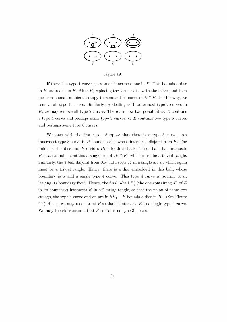
1 2 3
4 5 6
Figure 19.
If there is a type 1 curve, pass to an innermost one in E. This bounds a disc
in P and a disc in E. Alter P , replacing the former disc with the latter, and then
perform a small ambient isotopy to remove this curve of E ∩ P . In this way, we
remove all type 1 curves. Similarly, by dealing with outermost type 2 curves in
E, we may remove all type 2 curves. There are now two possibilities: E contains
a type 4 curve and perhaps some type 3 curves; or E contains two type 5 curves
and perhaps some type 6 curves.
We start with the first case. Suppose that there is a type 3 curve. An
innermost type 3 curve in P bounds a disc whose interior is disjoint from E. The
union of this disc and E divides B1 into three balls. The 3-ball that intersects
E in an annulus contains a single arc of B1 ∩ K, which must be a trivial tangle.
Similarly, the 3-ball disjoint from ∂B1 intersects K in a single arc α, which again
must be a trivial tangle. Hence, there is a disc embedded in this ball, whose
boundary is α and a single type 4 curve. This type 4 curve is isotopic to α,
leaving its boundary fixed. Hence, the final 3-ball B′1 (the one containing all of E
in its boundary) intersects K in a 2-string tangle, so that the union of these two
strings, the type 4 curve and an arc in ∂B1 −E bounds a disc in B′1. (See Figure
20.) Hence, we may reconstruct P so that it intersects E in a single type 4 curve.
We may therefore assume that P contains no type 3 curves.
31
B'1
B1
aE
Figure 20.
We claim that the ‘satellite’ tangle in B′1 is trivial. In other words, pair
(B′1, B
′1∩K) is homeomorphic to the product of an interval and the pair (E, E∩K).
The tangle in B′1 has a diagram which is a subset of the alternating diagram
D. However, a non-trivial satellite tangle cannot have an alternating diagram.
Otherwise, we could extend the tangle to an alternating diagram of a prime non-
trivial satellite knot, contradicting Menasco’s theorem [10]. This proves the claim.
We may now use the product structure on B′1 to isotope S, as required, across B′
1,
so that afterwards S has a simple arrangement in the diagram.
We now deal with the case where P intersects E in two type 5 curves and
possibly some type 6 curves. If there is a type 6 curve, consider one outermost
in P . This separates off a subdisc P ′ of P that is disjoint from K. It lies in
one component B′1 of cl(B1 − E). It separates the two arcs of B′
1 ∩ K. The
intersection between K and each component of B′1−P ′ is a trivial 1-string tangle.
Since ∂P ′ runs over E in a single arc, we deduce again that the pair (B′1, B
′1 ∩K)
is homeomorphic to the product of an interval and the pair (E, E∩K). Similarly,
if there are no type 6 curves, the closures of both components of B−E have such a
product structure. Hence, again, there is an ambient isotopy, leaving K invariant
and introducing no new points of S ∩K, taking S to the 2-sphere (S − ∂B′1) ∪E,
which has a simple arrangement with the knot diagram.
Hence, we may assume that S ∩ S2± is a single simple closed curve containing
all four points of S ∩ K.
32
In the case where the tubes of F are not nested, the proof of Theorem 2 is
now complete. Up to isotopy, the unknotting tunnel lies in the rational tangle B1
as shown in Figure 21. This is a planar arc in the diagram.
tunnel
Rational tangle
Figure 21.
Step 7. The case where the tubes are nested.
Recall from Step 5 that S divides S3 into B1 and B2. The tangle (B1, B1∩K)
is rational. We now need to analyse the other tangle (B2, B2 ∩K). We know that
F is a Heegaard surface for K. Hence, the component H ′ of S3 − int(N (F ))
containing K is obtained by attaching a 1-handle to a solid torus in which K is
the core curve. There is therefore an annulus A′ embedded in this handlebody
H ′, with K as one boundary component and the other boundary component lying
in ∂H ′. If D1 is the first meridional compression disc for F , we may assume that
D1∩A′ is a single arc running from ∂D1 to D1∩K. Hence, D′ = A′− int(N (D1))
is a disc lying on one side of T , such that D′∩(T ∪K) = ∂D′, with ∂D′ comprising
an arc in K and an arc in T . Note also that T has a compression disc disjoint from
K on the D′ side of T . Therefore, the component of S3 − int(N (T )) containing
D′ is a solid torus V , and K ∩ V is a curve α3 parallel to an arc in ∂V , via the
disc D′. This solid torus is B2 − int(N (α2)). We will exhibit a planar arc t with
endpoints in α3 such that α3 ∪ t is the union of a core curve in V and two vertical
arcs. This t will therefore be isotopic to the original unknotting tunnel.
Now, B2 − int(N (α2 ∪ α3)) is a handlebody. We may view the subset of the
diagram that specifies B2 as an alternating diagram for this handlebody, where
the outside of B2 is a single vertex. This diagram need not be reduced, since it
may be as in the right-hand diagram of Figure 5. But nevertheless, we deduce
from Theorem 3 that the diagram for B2 is either rational or as shown in Figure
33
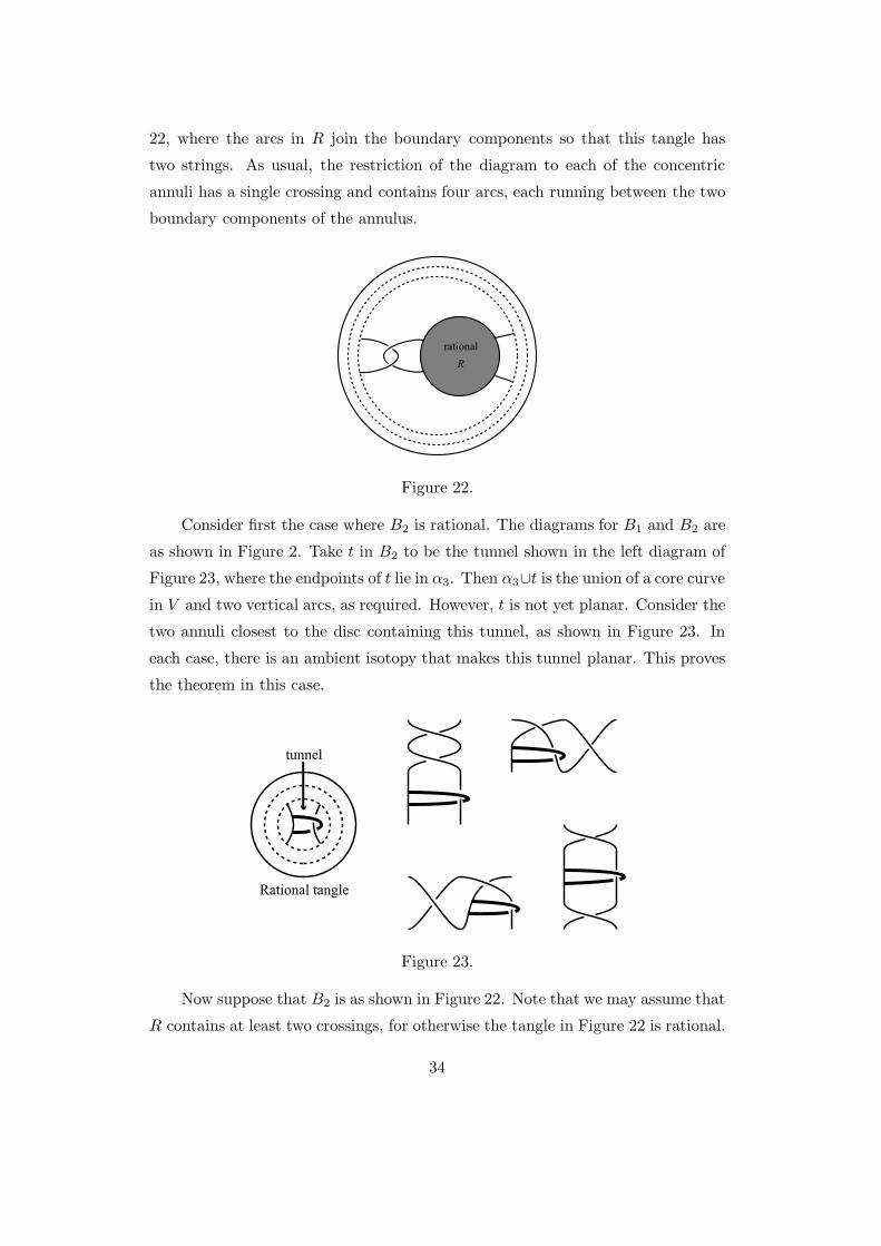
22, where the arcs in R join the boundary components so that this tangle has
two strings. As usual, the restriction of the diagram to each of the concentric
annuli has a single crossing and contains four arcs, each running between the two
boundary components of the annulus.
rationalR
Figure 22.
Consider first the case where B2 is rational. The diagrams for B1 and B2 are
as shown in Figure 2. Take t in B2 to be the tunnel shown in the left diagram of
Figure 23, where the endpoints of t lie in α3. Then α3∪t is the union of a core curve
in V and two vertical arcs, as required. However, t is not yet planar. Consider the
two annuli closest to the disc containing this tunnel, as shown in Figure 23. In
each case, there is an ambient isotopy that makes this tunnel planar. This proves
the theorem in this case.
tunnel
Rational tangle
Figure 23.
Now suppose that B2 is as shown in Figure 22. Note that we may assume that
R contains at least two crossings, for otherwise the tangle in Figure 22 is rational.
34
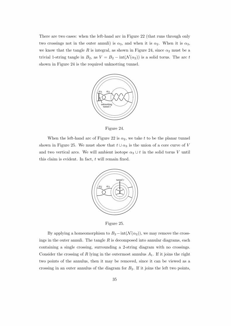
There are two cases: when the left-hand arc in Figure 22 (that runs through only
two crossings not in the outer annuli) is α3, and when it is α2. When it is α3,
we know that the tangle R is integral, as shown in Figure 24, since α2 must be a
trivial 1-string tangle in B2, as V = B2 − int(N (α2)) is a solid torus. The arc t
shown in Figure 24 is the required unknotting tunnel.
a a3 2
unknottingtunnel t
Figure 24.
When the left-hand arc of Figure 22 is α2, we take t to be the planar tunnel
shown in Figure 25. We must show that t ∪ α3 is the union of a core curve of V
and two vertical arcs. We will ambient isotope α3 ∪ t in the solid torus V until
this claim is evident. In fact, t will remain fixed.
a a2 3�
tunnel t
Figure 25.
By applying a homeomorphism to B2− int(N (α2)), we may remove the cross-
ings in the outer annuli. The tangle R is decomposed into annular diagrams, each
containing a single crossing, surrounding a 2-string diagram with no crossings.
Consider the crossing of R lying in the outermost annulus A1. If it joins the right
two points of the annulus, then it may be removed, since it can be viewed as a
crossing in an outer annulus of the diagram for B2. If it joins the left two points,
35
then we may flype R so that it lies between the right two points, and then remove
it. The cases where the crossing joins the top two points, and where it joins the
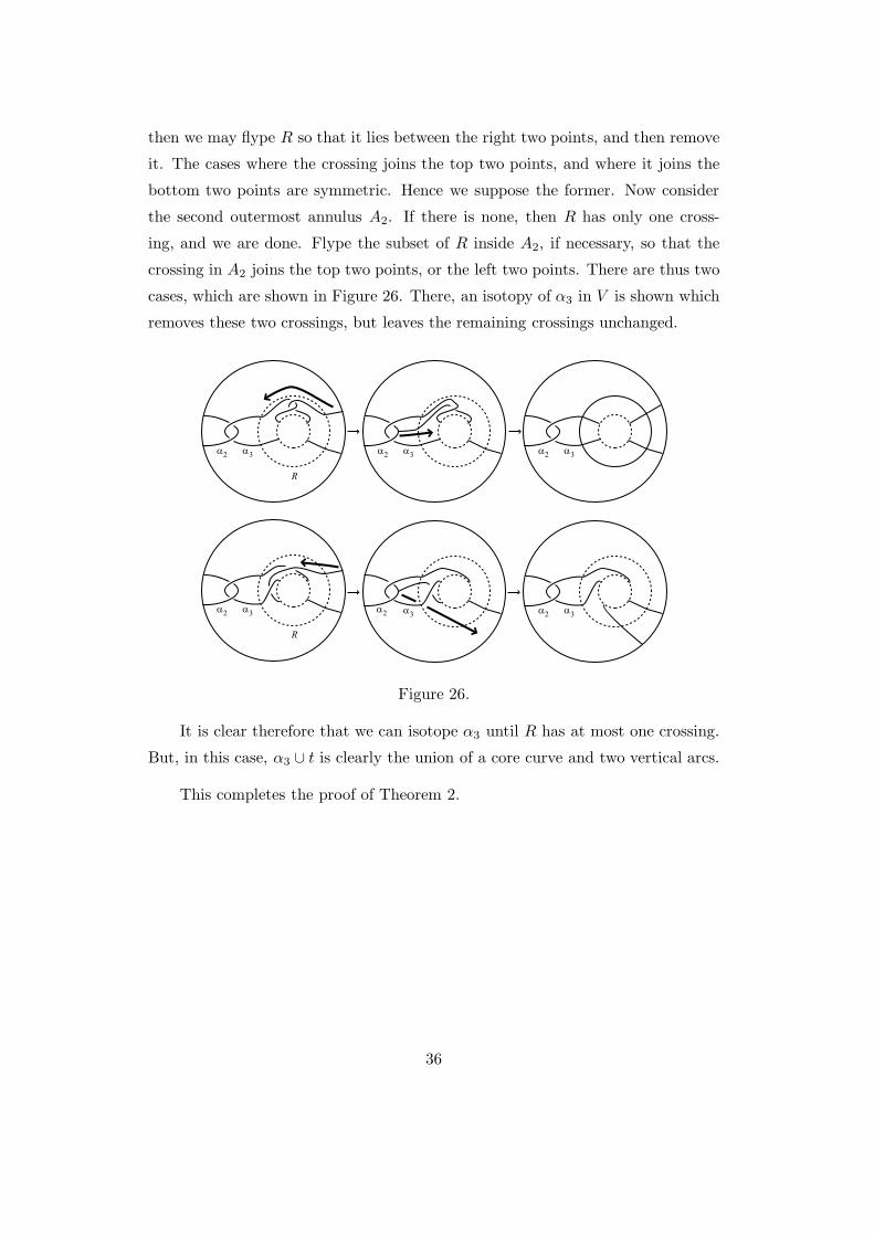
bottom two points are symmetric. Hence we suppose the former. Now consider
the second outermost annulus A2. If there is none, then R has only one cross-
ing, and we are done. Flype the subset of R inside A2, if necessary, so that the
crossing in A2 joins the top two points, or the left two points. There are thus two
cases, which are shown in Figure 26. There, an isotopy of α3 in V is shown which
removes these two crossings, but leaves the remaining crossings unchanged.
R
a a2 3�
R
a a2 3
a a2 3 a a2 3
a a2 3 a a2 3
Figure 26.
It is clear therefore that we can isotope α3 until R has at most one crossing.
But, in this case, α3 ∪ t is clearly the union of a core curve and two vertical arcs.
This completes the proof of Theorem 2.
36
References
1. G. BURDE and H. ZIESCHANG, Knots, de Gruyter (1985)
2. A. CASSON and C. GORDON, Reducing Heegaard splittings, Topology and
its Appl. 27 (1987) 275–283.
3. R. CROWELL, Genus of alternating link types, Ann. of Math. (2) 69 (1959)
258–275.
4. C. GORDON and A. REID, Tangle decompositions of tunnel number one
knots and links, J. Knot Theory Ramifications 4 (1995) 389–409.
5. J. HEMPEL, 3-Manifolds, Ann. of Math. Studies, No. 86, Princeton Univ.
Press, Princeton, N. J. (1976)
6. W. JACO and U. OERTEL, An algorithm to decide if a 3-manifold is Haken,
Topology 23 (1984) 195–209.
7. L. KAUFFMAN, State models and the Jones polynomial, Topology 26 (1987)
395–407.
8. T. KOBAYASHI, Classification of unknotting tunnels for two bridge knots.
Proceedings of the Kirbyfest (Berkeley, CA, 1998), 259–290 Geom. Topol.
Monogr., 2, Geom. Topol., Coventry (1999).
9. W. MENASCO, Polyhedra representation of link complements, Low-
dimensional Topology, Contemp. Math 20, Amer. Math. Soc. (1983) 305–
325.
10. W. MENASCO, Closed incompressible surfaces in alternating knot and link
complements, Topology 23 (1984) 37–44.
11. W. MENASCO and M. THISTLETHWAITE, Surfaces with boundary in al-
ternating knot exteriors, J. Reine Angew. Math. 426 (1992) 47–65.
12. K. MURASUGI, On the genus of the alternating knot. I, II, J. Math. Soc.
Japan 10 (1958) 94–105, 235–248.
13. K. MURASUGI, Jones polynomials and classical conjectures in knot theory,
Topology 26 (1987) 187–194.
37
14. J. H. RUBINSTEIN, Polyhedral minimal surfaces, Heegaard splittings and
decision problems for 3-dimensional manifolds, Proceedings of the Georgia