79
Department of Automatic Control Classification of EEG data using machine learning techniques Martin Heyden

Department of Automatic Control
Classification of EEG data using machine learning techniques
Martin Heyden

MSc Thesis TFRT-6019 ISSN 0280-5316
Department of Automatic Control Lund University Box 118 SE-221 00 LUND Sweden
© 2016 by Martin Heyden. All rights reserved. Printed in Sweden by Tryckeriet i E-huset Lund 2016

Abstract
Automatic interpretation of reading from the brain could allow for many interest-ing applications including movement of prosthetic limbs and more seamless man-machine interaction.
This work studied classification of EEG signals used in a study of memory. The goalwas to evaluate the performance of the state of the art algorithms. A secondary goalwas to try to improve upon the result of a method that was used in a study similarto the one used in this work.
For the experiment, the signals were transformed into the frequency domain andtheir magnitudes were used as features. A subset of these features was then selectedand fed into a support vector machine classifier. The first part of this work tried toimprove the selection of features that was used to discriminate between differentmemory categories. The second part investigated the uses of time series as featuresinstead of time points.
Two feature selection methods, genetic algorithm and correlation-based, were im-plemented and tested. Both of them performed worse than the baseline ANOVAmethod.
The time series classifier also performed worse than the standard classifier. How-ever, experiments showed that there was information to gain by using the time se-ries, motivating more advanced methods to be explored.
Both the results achieved by this thesis and in other work are above chance. How-ever, high accuracies can only be achieved at the cost of long delays and few outputalternatives. This limits the information that can be extracted from the EEG sensorand its usability.
3


Acknowledgements
Thanks to Inês Bramão and Mikael Johansson at the Department of PsychologyLund University, for answering my questions and making this project a possibility.
Thanks to everyone involved in the project at LTH: Bo Bernhardsson, AndersRobertsson and Michelle Chong for their guidance and helpful feedback.
Thanks to Johan Eker at Ericsson for many good discussions.
Thanks to the Department of Automatic Control for giving me an inspiring workenvironment.
5


Contents
1. Introduction 91. Motivation . . . . . . . . . . . . . . . . . . . . . . . . . . . . . 92. Project Partners . . . . . . . . . . . . . . . . . . . . . . . . . . 103. The Data . . . . . . . . . . . . . . . . . . . . . . . . . . . . . . 114. Challenges . . . . . . . . . . . . . . . . . . . . . . . . . . . . . 115. Goals . . . . . . . . . . . . . . . . . . . . . . . . . . . . . . . . 146. Report Outline . . . . . . . . . . . . . . . . . . . . . . . . . . . 14
2. Brain Computer Interface Overview 151. Introduction . . . . . . . . . . . . . . . . . . . . . . . . . . . . 152. BCI as a Classification System . . . . . . . . . . . . . . . . . . 163. Sources . . . . . . . . . . . . . . . . . . . . . . . . . . . . . . . 174. Preprocessing . . . . . . . . . . . . . . . . . . . . . . . . . . . 195. Features . . . . . . . . . . . . . . . . . . . . . . . . . . . . . . 196. Different types of BCI systems . . . . . . . . . . . . . . . . . . 237. State of the art . . . . . . . . . . . . . . . . . . . . . . . . . . . 24
3. Classification 251. Introduction . . . . . . . . . . . . . . . . . . . . . . . . . . . . 252. Example of some classifiers . . . . . . . . . . . . . . . . . . . . 273. Algorithm independent theory . . . . . . . . . . . . . . . . . . . 334. Support Vector Machines . . . . . . . . . . . . . . . . . . . . . 365. Time Series Classification using SVM . . . . . . . . . . . . . . 426. BCI classification . . . . . . . . . . . . . . . . . . . . . . . . . 44
4. Feature Reduction 461. Introduction . . . . . . . . . . . . . . . . . . . . . . . . . . . . 462. ANOVA . . . . . . . . . . . . . . . . . . . . . . . . . . . . . . 473. Correlation-Based Feature Selection . . . . . . . . . . . . . . . 494. Genetic Algorithm . . . . . . . . . . . . . . . . . . . . . . . . . 52
5. Experimental Setup 571. The Study . . . . . . . . . . . . . . . . . . . . . . . . . . . . . 572. Classification Setup . . . . . . . . . . . . . . . . . . . . . . . . 59
7

Contents
3. Previous Work . . . . . . . . . . . . . . . . . . . . . . . . . . . 616. Method 63
1. Software . . . . . . . . . . . . . . . . . . . . . . . . . . . . . . 632. Static Classifier . . . . . . . . . . . . . . . . . . . . . . . . . . 633. Dynamic Classifier . . . . . . . . . . . . . . . . . . . . . . . . . 66
7. Results 681. Static Classifier . . . . . . . . . . . . . . . . . . . . . . . . . . 682. Dynamic Classifier . . . . . . . . . . . . . . . . . . . . . . . . . 71
8. Discussion and Conclusions 721. Conclusions . . . . . . . . . . . . . . . . . . . . . . . . . . . . 722. Discussion . . . . . . . . . . . . . . . . . . . . . . . . . . . . . 723. Future Work . . . . . . . . . . . . . . . . . . . . . . . . . . . . 73
Bibliography 74
8
1Introduction
1. Motivation
The human body is very capable of interacting with its surrounding. It can shareits thoughts by speaking and move around via muscles. In some cases this is notpossible due to disabilities or injuries. In other cases it would be beneficial if thebrain could interact directly with its surrounding without first having to go throughthe rest of the body. For example activating an emergency button at the moment thebrain wants to could be faster than the person physically having to press it.
This might sound like science fiction but the technology is not that far away. Oneway for the neurons in the brain to communicate is through electrical activity. Thoseelectrical activities will change depending of what the brain is trying to accomplish.If that activity can be measured and interpreted, the intentions of a person could beread without relying on the rest of his body.
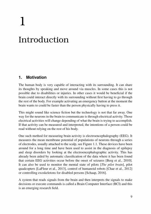
One such method for measuring brain activity is electroencephalography (EEG). Itmeasures the mean membrane potential of populations of neurons through a seriesof electrodes, usually attached to the scalp, see Figure 1.1. These devices have beenaround for a long time and have been used to assist in the diagnosis of epilepsyand sleep disorders by looking at the electroencephalographic activity. This hasalready been aided by automatic classification of the data where it has been foundthat certain EEG activities occur before the onset of seizures [Berg et al., 2010].It can also be used to monitor the mental state of pilots [The pilot brain], pilotquadcopters [LaFleur et al., 2013], control of humanoid robots [Chae et al., 2012]or controlling exoskeletons for disabled persons [Schaap, 2016].
A system that reads signals from the brain and then interprets the signals to makedecisions or execute commands is called a Brain Computer Interface (BCI) and thisis an emerging research field.
9

Chapter 1. Introduction
Figure 1.1 A cap used for EEG measurements. The measurements areread from a series of electrodes placed evenly over the head. Taken fromhttp://www.flickr.com/photos/tim_uk/8135755109/.
2. Project Partners
This project has been a cooperation between three entities: The Department of Psy-chology at Lund University, the Department of Automatic Control at Lund Uni-versity and Ericsson Research. Different goals were envisioned by each entitiy, butit was believed that they could be combined into one project. These goals are de-scribed below.
The psychology department is conducting research within memory research andspecifically, in the mechanism of memory creation and retrieval.
When someone is trying to remember something, the memory is said to be encodedby the brain. When that memory is later being remembered, it is said to be recol-lected. An interesting question is if the processes that happens during the encodingof a memory is later replayed during recollection. One way of testing this is to see ifpatterns present during encoding is also present during recollection [Jafarpour et al.,2014].
There is currently no unifying theory for how this process work [Widmaier et al.,2014].
The Department of Automatic Control is interested in using the EEG as a sensor inrobotics applications. It could also be used as a sensor in vehicles as a safety systemto monitor the state and intentions of the driver.
Ericsson is interested in finding new sensors and techniques that can be utilized withthe help of the new 5G technology. The EEG sensor could then be wireless and thecalculations done in the cloud. It could also be an interesting part of the internet ofthings.
10

3. The Data
Figure 1.2 Example of images used in the memory study used in this project. The picturescome from three different categories: objects, faces and landmarks. The participants are askedto try to memorize word/picture pairs and are later asked to recall the picture when presentedwith the word. [Image source: Inês Bramão, Department of Psychology, Lund University.]
3. The Data
The data for this project was supplied by the Department of Psychology at LundUniversity and was designed to study if patterns during encoding emerged duringrecollection.
The study consisted of the participants trying to remember word-picture pairs. Thepicture was from three categories: faces, landmarks and, objects. An example of thepictures used in the study is depicted in Figure 1.2.
EEG measurements were recorded during the entire experiment. However, only therecordings from memorization were used in this work. More details about the datais given in Chapter 5.
4. Challenges
It is challenging to automatically classify EEG signals due to the problems withthe signals described below. Advances in computing power, signal processing, ma-chine learning, and EEG reading devices have however increased the capabilities ofautomatic interpretations of the results.
The SignalsElectroencephalography (EEG) uses electrodes placed over the skull to measureelectric activity in the brain.
A conductive gel is usually applied to the electrodes to improve reading quality. Foran every day BCI system this is not feasible. And even then the EEG measurementsare on the µV scale and have low signal-to-noise ratio. The signals are further cor-rupted by artifacts, electrical signals originating from, for example, eye and muscle
11

Chapter 1. Introduction
−1.5 −1 −0.5 0 0.5 1 1.5 2 2.5−40
−30
−20
−10
0
10
20
30
µ V
seconds
Figure 1.3 Plot of EEG readings from one of the channels during the memory experiment.Notice that it is on the magnitude of micro Volts and that at least two different frequencycomponents can be seen.
movement. These artifacts might be much stronger than the electrical activity that isstudied. The signals also often have multiple different frequency components evenin the absence of artifacts. Another problem is the limited spatial resolution.
The strength of EEG lies in its high temporal resolution and that it is cheaper andmore portable than many other brain imaging techniques.
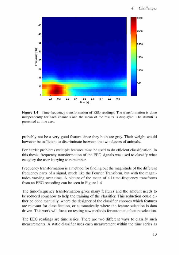
An example of the readings from channel 24 can be seen in Figure 1.3. It can beseen that there are at least two different frequencies present. Notice also the lowamplitude of the magnitude of ten micro Volts.
Classification and feature selectionThis work will focus on the problem of classification. The goal of classification isto use measurements to decide what the source of the measurements is. Choosingwhat measurements to use is a large part of the problem. The chosen measurementsare called features. The different sources are called classes.
When trying to classify between a mouse and an elephant there are many possiblemeasurements. One could measure the color of the animals presented but that would
12
4. Challenges
Figure 1.4 Time-frequency transformation of EEG readings. The transformation is doneindependently for each channels and the mean of the results is displayed. The stimuli ispresented at time zero.
probably not be a very good feature since they both are gray. Their weight wouldhowever be sufficient to discriminate between the two classes of animals.
For harder problems multiple features must be used to do efficient classification. Inthis thesis, frequency transformation of the EEG signals was used to classify whatcategory the user is trying to remember.
Frequency transformation is a method for finding out the magnitude of the differentfrequency parts of a signal, much like the Fourier Transform, but with the magni-tudes varying over time. A picture of the mean of all time-frequency transformsfrom an EEG recording can be seen in Figure 1.4
The time-frequency transformation gives many features and the amount needs tobe reduced somehow to help the training of the classifier. This reduction could ei-ther be done manually, where the designer of the classifier chooses which featuresare relevant for classification, or automatically where the feature selection is datadriven. This work will focus on testing new methods for automatic feature selection.
The EEG readings are time series. There are two different ways to classify suchmeasurements. A static classifier uses each measurement within the time series as
13

Chapter 1. Introduction
a feature, and does not use the time information. A dynamic classifier instead useseach time series as a feature. Both type of classifiers were studied in this thesis.
5. Goals
This thesis will focus on two tasks.
The first task was to get an overview of the state of the art of EEG classification andunderstand what methods are being used. This work is presented in chapters 2 and3. While some methods was described in detail there was no time for a thoroughtheoretical handling of all methods being found. The interested reader can readfurther in the references given for methods that were not described with enoughdetail.
The second task was to design an EEG classifier for the encoding phase of thememory study. First a classifier that was previously used in similar research wasimplemented as baseline. Then two new classifiers using different feature selectionwere then implemented with the goal of improving on the baseline.
LimitationsIn a field as big as brain computer interface there had to be limitations on whatwas explored. In this project there was only one feature type, power spectral densityvia continuous wavelet transform. There was also only one classifier type, supportvector machines. These were used in previous work. Instead, only feature selectionmethods were explored. The usage of an SVM is also motivated by its convexity.Always finding a global maximum for the design of the classifier is very convenientwhen testing feature selection methods.
There were many possible techniques to explore in this project. Some notable thathad to be discarded due to time constraint included outlier rejection or to weightsamples differently. Deep learning techniques were also not explored.
6. Report Outline
Chapter 2 gives an overview of the BCI field. Chapter 3 covers classification andChapter 4 covers the feature reduction method used in this work. Chapter 5 de-scribes the experiment in detail and the framework used for classification. Chapter 6describes the method used in this thesis and their results are presented in Chapter 7.The final discussion and suggestion for future work is given in Chapter 8.
14
2Brain Computer InterfaceOverview
1. Introduction
A Brain Computer Interface (BCI) is a system that takes inputs from the brain, forexample EEG, and translates it to commands on a computer. This is usually doneby classification, where several commands are trained. The training consists of theuser executing the different commands. The goal is then to build a system whichuses this information to classify future commands.
This work will not look into model-based EEG classification. This has been donefor seizure detection [Chong, 2013] where the signals are much stronger than forordinary brain activity. It is not assumed to be impossible to use a model-basedapproach for normal signals, but such possibilities were not explored.
Instead of making a new literature study, results will be presented from Hwang etal. [Hwang et al., 2013] that reviews the literature from 2007 to 2011. It does notinclude the most recent research but should still be sufficient for giving an overviewof the field.
An illustration of a complete BCI system can be seen in Figure 2.1. The first step issignal acquisition where data is acquired, for example via EEG. Next features areextracted from the data and commands are decided based on those features.
Memory classification is not a BCI system since there are no commands executed.Everything up the the command execution is however the same, and the executionof commands is generally not the hard part of building a BCI system. Memoryclassification will hence be treated as a BCI system throughout this report.
15

Chapter 2. Brain Computer Interface Overview
Figure 2.1 An overview of an BCI system taken from [Thorpe et al., 2005]. The signal ac-quisition might for example be from EEG signals. Features are then extracted and translatedto commands via, for example, machine learning.
2. BCI as a Classification System
The following properties and problems need to be considered for all BCI systemsthat rely on classification [Lotte et al., 2007].
Noise and Outliers: BCI features are very noisy and might contain outliers due tothe poor signal-to-noise ratio of EEG signals (or other measurement meth-ods).
High Dimensionality: Due to the many channels and potential features per chan-nel the feature vectors for BCI systems are usually of very high dimension.This can be handled by feature reduction or by a classification method thatcan handle many features.
Time Information: BCI contains information over time. This could be handledby concatenating feature vectors for different time points or classifying timeseries.
16
3. Sources
Non stationary: EEG signals often vary over time, and it might even be the changethat is interesting.
Small training sets: It is usually very time consuming to get large training sets.This is usually not feasible since the test-person could get fatigued. Hencethe classifier method needs to work well even with a low number of trainingdata.
3. Sources
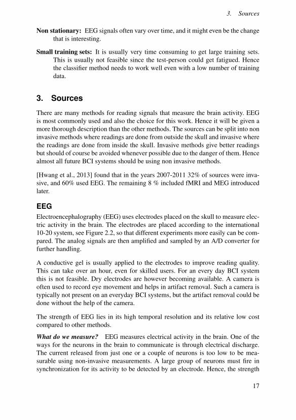
There are many methods for reading signals that measure the brain activity. EEGis most commonly used and also the choice for this work. Hence it will be given amore thorough description than the other methods. The sources can be split into noninvasive methods where readings are done from outside the skull and invasive wherethe readings are done from inside the skull. Invasive methods give better readingsbut should of course be avoided whenever possible due to the danger of them. Hencealmost all future BCI systems should be using non invasive methods.
[Hwang et al., 2013] found that in the years 2007-2011 32% of sources were inva-sive, and 60% used EEG. The remaining 8 % included fMRI and MEG introducedlater.
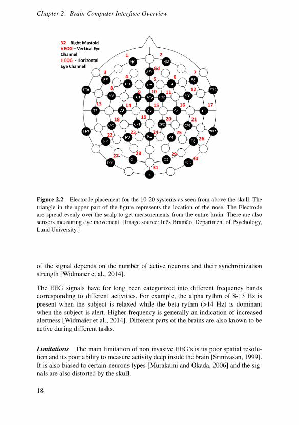
EEGElectroencephalography (EEG) uses electrodes placed on the skull to measure elec-tric activity in the brain. The electrodes are placed according to the international10-20 system, see Figure 2.2, so that different experiments more easily can be com-pared. The analog signals are then amplified and sampled by an A/D converter forfurther handling.
A conductive gel is usually applied to the electrodes to improve reading quality.This can take over an hour, even for skilled users. For an every day BCI systemthis is not feasible. Dry electrodes are however becoming available. A camera isoften used to record eye movement and helps in artifact removal. Such a camera istypically not present on an everyday BCI systems, but the artifact removal could bedone without the help of the camera.
The strength of EEG lies in its high temporal resolution and its relative low costcompared to other methods.
What do we measure? EEG measures electrical activity in the brain. One of theways for the neurons in the brain to communicate is through electrical discharge.The current released from just one or a couple of neurons is too low to be mea-surable using non-invasive measurements. A large group of neurons must fire insynchronization for its activity to be detected by an electrode. Hence, the strength
17
Chapter 2. Brain Computer Interface Overview
32 – Right Mastoid VEOG – Vertical Eye Channel HEOG Horizontal Eye Channel
1 2
3 4 5
Gd
6 7
8 10 11
12
13 14 15 16 17
18 19 20 21
22 23 24 25
26
27 30
31
28 29
9
Figure 2.2 Electrode placement for the 10-20 systems as seen from above the skull. Thetriangle in the upper part of the figure represents the location of the nose. The Electrodeare spread evenly over the scalp to get measurements from the entire brain. There are alsosensors measuring eye movement. [Image source: Inês Bramão, Department of Psychology,Lund University.]
of the signal depends on the number of active neurons and their synchronizationstrength [Widmaier et al., 2014].
The EEG signals have for long been categorized into different frequency bandscorresponding to different activities. For example, the alpha rythm of 8-13 Hz ispresent when the subject is relaxed while the beta rythm (>14 Hz) is dominantwhen the subject is alert. Higher frequency is generally an indication of increasedalertness [Widmaier et al., 2014]. Different parts of the brains are also known to beactive during different tasks.
Limitations The main limitation of non invasive EEG’s is its poor spatial resolu-tion and its poor ability to measure activity deep inside the brain [Srinivasan, 1999].It is also biased to certain neurons types [Murakami and Okada, 2006] and the sig-nals are also distorted by the skull.
18

4. Preprocessing
Other methodsBelow follows a short introduction to other methods to measure brain activity.
MEG Magnetoencephalography (MEG) is a technique similar to EEG, but it readsthe magnetic fields induced by the current in the brain.
MEG typically has hundreds of channels. Furthermore its magnetic readingsare less distorted than the electric potential of EEG by the skull.
MEG requires shielding from magnetic fields, including the earth’s. Thismeans that it can only be used in controlled environments such as in clini-cal applications.
fMRI Functional magnetic resonance imaging measures brain activity by detectingchanges in blood flow. It uses the principle that active areas in the brain haveincreased blood flow. The blood flow is detected using a strong magneticfield to align the oxygen nuclei and another field to to locate the nuclei. Themethod has very high spatial resolution, pinpointing the location in 3d-space,but has low time resolution.
Invasive methods Invasive methods involve taking measurements under the skull.The benefit is that the signals do not get distorted by the skull. It is howevera very dangerous procedure and should only be used when necessary.
4. Preprocessing
The EEG signal comes with a lot of noise. Contracting muscles or even movingthe eyes will result in big changes in the signal. Because of this the signals need tobe cleaned up from such artifacts. In clinical applications this is usually done by acombination of independent component analysis, which tries to separate the signalinto independent components [Lee, 1998], and visual inspection. For a BCI systemthere is no time for manual intervention and the clean up needs to be automated.
Automatic artifact removal is necessary for a BCI system but will not be covered inthis work.
5. Features
There are many different possible features to use for classifying EEG signals. Abrief overview of methods used in the field will be given, but for details please seethe references given below. As this project only considered one type of featuresthere will be no discussion of the different features strength and weaknesses due totime constraints.
19

Chapter 2. Brain Computer Interface Overview
Figure 2.3 Overview of features used in BCI research. [Hwang et al., 2013]
FrequencyThe Fourier transform of a signal x(t) defined for all t ∈ R is given by
X( f ) =∫
∞
−∞
x(t)e−i2π f t dt. (2.1)
The spectrogram of x(t) is given by S( f ) = |X( f )|2 and serves as an estimationof the magnitude of different frequencies. This method has two obvious problems.Firstly, it requires data on an infinite time domain, and secondly, the frequency isthe same for all time points. These two problems are attempted to be solved by theso called short time Fourier transform which uses a window w to locally calculatean approximation of the Fourier transform.
X(τ, f ) =∫
∞
−∞
x(t)w(t− τ)e−i2π f t dt (2.2)
The window function is usually symmetric and of unit L2 norm. The spectrogramnow has a time component and is calculated as S(t, f ) = |X(t, f )|2. For further treat-ment see [Sandsten, 2016].
For a window function with support in a finite interval, infinite future samples areno longer needed, but for calculations for time t there still must be measurementsup to time t +∆ where ∆ depends on the support of the window function. Lowerfrequencies require larger delays.
20

5. Features
Since the data will be used in a computer there is no use for continuous frequencymeasurements. The short time Fourier transform has a discrete counterpart
X(m, f ) =∞
∑n=−∞
x[n]w[n−m]e−i2πn (2.3)
There are many ways to calculate the frequencies of the signals. Some of thosemethods will be briefly introduced here for completeness, but this work does notattempt to find the best method or finding the best configuration for the method ofchoice.
Multitapers Multitapers use several independent windows to estimate from thesame data segment. The final estimation is then the average of all windows whichreduces the variance of the estimation, see [Percival and Walden, 1993] for furthertreatment.
Continuous Wavelets One limitation of the short time Fourier transform is that ituses the same window function for all frequencies. Using a big window functionwill lead to bad time resolution and a small window will lead to bad frequencyresolution. The continuous wavelet transform of x(t) is calculated using a waveletfunction ψs,t0(t)
W (s, t0) =∫
∞
−∞
x(t)ψ∗s,t0(t) dt, (2.4)
where x∗ denotes the complex conjugate of x, t0 is the center of the windows and sis the timescale. For some windows s = 1
f but this is generally not true. The waveletis calculated from the mother wavelet
ψs,t0(t) =1√s
ψ0
(t− t0
s
). (2.5)
Notice how the wavelet gets smaller for larger frequencies. See [Hramov et al.,2015] for further discussion.
Autoregressive coefficentsAn autoregressive (AR) model is used to describe a random process where the nextvalue depends linearly on some of the previous values, and a white noise e. For ascalar AR model of order p this can be described as
x[t] =p
∑i=1
αix[t− i]+ e[t]. (2.6)
21

Chapter 2. Brain Computer Interface Overview
For further discussion and how to calculate the coefficents αi, see [Jakobsson,2013]. For EEG this needs to be extended to be time varying and multivariate. Foran adaptive autoregressive process, αi(t) is a function of time. This was used in[Schlögl et al., 1997] where it was argued that the random nature of the processwell described the random nature of the EEG data.
The AR coefficents can then either directly be fed into a classifier or used for fre-quency estimation [Krusienski et al., 2006]
S(ei2π f ) =σ2
e
|1−∑pi=1 αie− j2π f |2
. (2.7)
where σe is the variance of the white noise e.
Hjorth parametersHjorth parameters were introduced by Bo Hjorth [Hjorth, 1970]. They consist ofthree quantities which can be defined in the frequency domain but which also canbe calculated in the time domain.
Activity: The variance, which is the same as the power, of the signal var(y(t)).
Mobility: Describes the mean frequency and is calculated as
mobility(y(t)) =
√√√√var(
dydt y(t)
)var(y(t))
(2.8)
Complexity: Describes the change in frequency and is calculated as
complexity(y(t)) =mobility
(dydt y(t)
)mobility(y(t))
(2.9)
Phase synchronizationMost frequency methods only look at the amplitude, ignoring the phase. AR coef-ficients also ignore the phase of the signals. The phase information could be veryrelevant since two parts of the brain having the same phase indicate that they arecooperating [Brunner et al., 2006]. There are multiple measures of synchronizationbut they will not be presented here.
Phase has not been popular in BCI research. This might partly be due to BCI be-ing a very m alsoulti-disciplinary research field and phase features require moremathematical involvement.
22
6. Different types of BCI systems
An example of when it is used is [Daly et al., 2012] where functional connectiv-ity is used. Functional connectivity is defined as communication between differentregions and is identified via phase synchronization.
Event-Related PotentialEvent-related potential (ERP) is the change in potential that happens due to stimuli.The most commonly used ERP is P300. P300 reacts to a visual stimuli and afterabout 300 ms the ERP can be observed. A common setup for a P300 BCI systemis a matrix of example letters where the user focuses on the one he or she wantsto write. Flashing the row or column of the desired letter elicits a P300 while theothers do not. The P300 ERP can be detected by spectral methods [Fazel-Rezai etal., 2012].
ERP is a common method in BCI research. However, it will not be discussed furthersince it is far from the rest of the work.
6. Different types of BCI systems
BCI systems can be split into different categories. What follows is a summary from[Nicolas-Alonso and Gomez-Gil, 2012]. The first distinction is between systemsthat rely on external stimuli and those that do not.
Exogenous: Exogenous BCI system uses neural activity that originates from exter-nal stimuli. This method have the advantage of requiring only one channel,very little training and having a bit rate of up to 60 bit/min. It does howeverrequire permanent attention to the stimuli, limiting its use in industrial appli-cations. A P300-based BCI system is an example of an exogenous system.
Endogenous: Endogenous BCI does not rely on any stimuli. It instead relies onthe user self regulating the brain rhythm. This technique has the advantage ofbeing operated when the user wants to, and without having to focus on thestimuli. It does however require a lot of training (weeks or months) wherethe trainie has to learn to produce specific patterns. This is done via neurofeedback, where the user is presented how close to a pattern he is. Multi-channel EEG recordings are also required for good performance. The bit rateis typically 20-30 bits/min. A system based on imagined movement is oneexample of an endogenous system.
BCI systems can further be split into synchronous, which only analysis the signalsduring pre defined time bins, and asynchronous, which always looks at the signalsseeing if there is a command present. Synchronous is much easier to implement, butasynchronous offers much more seamless interaction.
23

Chapter 2. Brain Computer Interface Overview
Endogenous asynchronous is the most interesting system, but also the hardest!
7. State of the art
This work did not have time for a complete overview of the start of the art results.Instead the current capabilities of the BCI technology will be highlighted by pre-senting some results in finger tapping classification.
Three properties of a BCI system are of interest: its speed, its accuracy, and thenumber of possible outputs. The bit rate, or information content the classifier isable to achieve depends on these three properties. A high bit rate is wanted, but ifthe accuracy of the system is too low, it will be unsatisfactory to use. No bit ratecalculation was done in this work.
Blankertz et al. [2006] achieved a mean accuracy of 89.5 % on imagined movementfor detection of continuous tapping over trials of 2 seconds. 128 EEG channels wereused which is a lot of channels. It did however require very little training with thehelp of presenting the user with feedback. The highest bit rate was at 35 bits/minwith an accuracy of 98 % while one subject had 15 bit per min and another couldnot achieve any BCI control, illustrating the variability in current BCI performance.
Ang et al. [2008] achieved an accuracy of 76.7 % on imagined taps on 2 secondintervals. This study used 118 electrodes.
The cited work above managed to achieve good accuracy, but at the cost of onlybeing able to detect continuous tapping, and only in segments of 2 seconds. Thiswould lead to very delayed control. Daley et al. [2011] tried to identify single imag-ined taps for different time intervals. For intervals of 1 second an accuracy slightlyabove 80 % was achieved. 0.5 second gave an accuracy around 63% and was thesmallest window that was significant above chance on a α = 0.01 level. This workonly used 19 channels.
It can be noted that high accuracy can only be achieved by low time resolution,limiting the information content that can be extracted from the sensor.
24
3Classification
1. Introduction
The goal of the classification in this work is to be able to distinguish between thethree different memory categories by using the EEG data. To do so, the computermust be able to recognize the different patterns that arise in the measurements of theelectrical potential of the brain. This is a standard problem in the field of machinelearning.
The problem could be viewed as a decision problem. The machine is presentedwith some data and is then expected to make a correct decision based on that data.Below follows some examples of general decision problems to illustrate the conceptof decision problems.
• Given a black jack hand, should the player hit or stand?
• Given measurements about wind and temperature, what will the temperaturebe in two days?
• Given a picture of a face, who is the person?
For a black jack hand, the decision could be made by understanding the mathematicsof blackjack. For the weather prediction, the prediction could be made explicitly bymodels of the weather which have been learned from previous experience. For facerecognition, it is common that the system has a set of training pictures which it usesto make a prediction when presented with a new picture. For all these examples it isclear that the decisions require some prior information about the problem.
In this work, the data was EEG signals and the goal was to make some decisionbased upon them. In general, that decisions could be where to move the cursor ona screen or how to move a prosthetic limb. Specifically in the memory experiment,
25
Chapter 3. Classification
the decision that had to be made was which of the three categories the user has triedto remember.
Old samples with known memory category will be used to classify new ones. This iscalled supervised classification and is the only machine learning technique that willbe used in this work. Supervised means that the labels of the training data are known.Classification means that the output of the learning system is discrete, for example"hit" or "stand". For regression based learning the output is instead continuous, fortemperature prediction the temperature could take on any value. For unsupervisedlearning the machine learning is presented with data samples with unknown label.Part of the learning task is to cluster which training data that belong together, forexample which pictures that depict the same person.
Outline of the Classification ProblemThe previous discussion is now formalized for the case of supervised classification.The task is to use a set of old training samples X = {~x i} to classify new samples~xnew. Each sample contains a set of features~x i = xi
1, ...,xin. Choosing a good feature
set is an important part of getting good classifier performance and will be discussedfurther in the next chapter.
Classification is made by designing a decision rule that assigns each feature vector~x to a class yi based on the samples in the training set. The decision rule can thenbe used to classify both old and new samples. Classifying the training set gives anaccuracy called the training accuracy.
The goal of the decision rule is to find the structure of the classes. A good trainingaccuracy is important as it can not be expected to do better on new data than onolder data. But it is the accuracy on a previously unseen set, called the testing test,that is the true measure of the classifier’s performance. That accuracy is often calledtesting accuracy. Using a model that is too complex will often lead to good trainingaccuracy, but bad testing accuracy as the model finds the structure in the training setinstead of the class structure.
Sometimes there are parameters in the classifier that have to be chosen by the user.These are sometimes chosen in a data driven fashion by splitting the data into threesets: Training, testing and evaluation. The classifier is trained on the training set fordifferent parameter configurations and evaluated on the testing sets. This could bedone by searching on a grid in the parameter space or by using some more advancedsearch technique. The classifiers are evaluated on the testing set and the one thatperforms best is then tested on the previously untouched evaluation set to yield itsgeneralization performance. Note that if the accuracy of the testing set was to beused the classifier would be evaluated on data it has already seen!
26
2. Example of some classifiers
0 1 2 3 4 5 6
1
2
3
4
5
Current(A)
Vol
tage(V
)
First order polynomialForth order polynomial
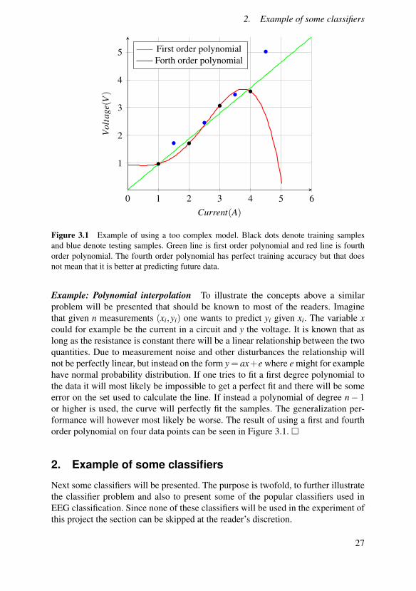
Figure 3.1 Example of using a too complex model. Black dots denote training samplesand blue denote testing samples. Green line is first order polynomial and red line is fourthorder polynomial. The fourth order polynomial has perfect training accuracy but that doesnot mean that it is better at predicting future data.
Example: Polynomial interpolation To illustrate the concepts above a similarproblem will be presented that should be known to most of the readers. Imaginethat given n measurements (xi,yi) one wants to predict yi given xi. The variable xcould for example be the current in a circuit and y the voltage. It is known that aslong as the resistance is constant there will be a linear relationship between the twoquantities. Due to measurement noise and other disturbances the relationship willnot be perfectly linear, but instead on the form y= ax+e where e might for examplehave normal probability distribution. If one tries to fit a first degree polynomial tothe data it will most likely be impossible to get a perfect fit and there will be someerror on the set used to calculate the line. If instead a polynomial of degree n− 1or higher is used, the curve will perfectly fit the samples. The generalization per-formance will however most likely be worse. The result of using a first and fourthorder polynomial on four data points can be seen in Figure 3.1. �
2. Example of some classifiers
Next some classifiers will be presented. The purpose is twofold, to further illustratethe classifier problem and also to present some of the popular classifiers used inEEG classification. Since none of these classifiers will be used in the experiment ofthis project the section can be skipped at the reader’s discretion.
27
Chapter 3. Classification
y
x
Figure 3.2 Example of Nearest neighbor classifier. Blue and red are the two differentclasses. Black indicate new samples that should be classified and the circle around themshow the closest neighbor. Note how old samples are used to classify new.
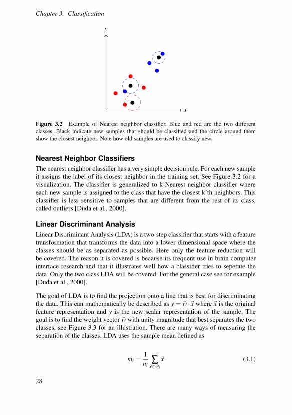
Nearest Neighbor ClassifiersThe nearest neighbor classifier has a very simple decision rule. For each new sampleit assigns the label of its closest neighbor in the training set. See Figure 3.2 for avisualization. The classifier is generalized to k-Nearest neighbor classifier whereeach new sample is assigned to the class that have the closest k’th neighbors. Thisclassifier is less sensitive to samples that are different from the rest of its class,called outliers [Duda et al., 2000].
Linear Discriminant AnalysisLinear Discriminant Analysis (LDA) is a two-step classifier that starts with a featuretransformation that transforms the data into a lower dimensional space where theclasses should be as separated as possible. Here only the feature reduction willbe covered. The reason it is covered is because its frequent use in brain computerinterface research and that it illustrates well how a classifier tries to seperate thedata. Only the two class LDA will be covered. For the general case see for example[Duda et al., 2000].
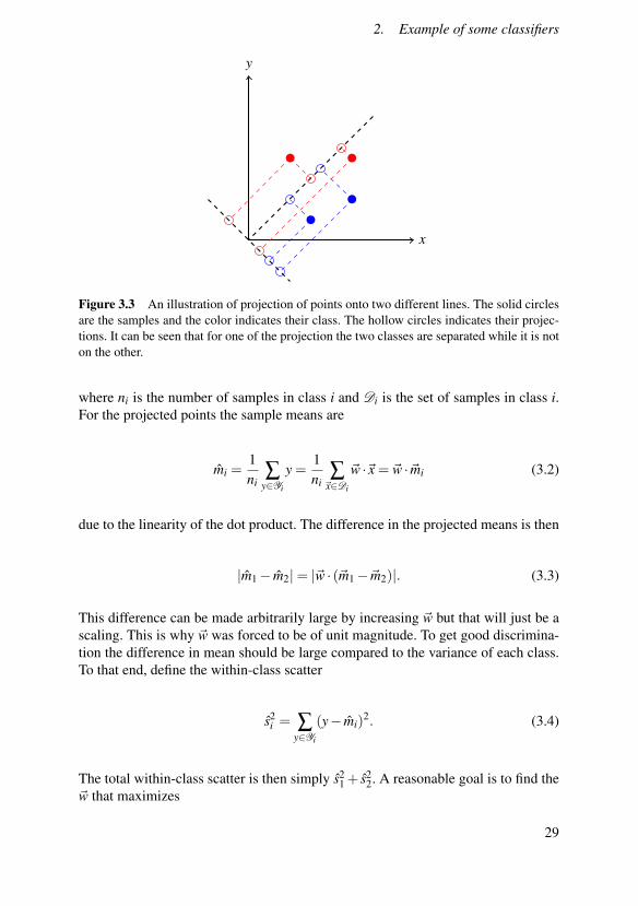
The goal of LDA is to find the projection onto a line that is best for discriminatingthe data. This can mathematically be described as y = ~w ·~x where ~x is the originalfeature representation and y is the new scalar representation of the sample. Thegoal is to find the weight vector ~w with unity magnitude that best separates the twoclasses, see Figure 3.3 for an illustration. There are many ways of measuring theseparation of the classes. LDA uses the sample mean defined as
~mi =1ni
∑~x∈Di
~x (3.1)
28
2. Example of some classifiers
y
x
Figure 3.3 An illustration of projection of points onto two different lines. The solid circlesare the samples and the color indicates their class. The hollow circles indicates their projec-tions. It can be seen that for one of the projection the two classes are separated while it is noton the other.
where ni is the number of samples in class i and Di is the set of samples in class i.For the projected points the sample means are
mi =1ni
∑y∈Yi
y =1ni
∑~x∈Di
~w ·~x = ~w ·~mi (3.2)
due to the linearity of the dot product. The difference in the projected means is then
|m1− m2|= |~w · (~m1−~m2)|. (3.3)
This difference can be made arbitrarily large by increasing ~w but that will just be ascaling. This is why ~w was forced to be of unit magnitude. To get good discrimina-tion the difference in mean should be large compared to the variance of each class.To that end, define the within-class scatter
s2i = ∑
y∈Yi
(y− mi)2. (3.4)
The total within-class scatter is then simply s21 + s2
2. A reasonable goal is to find the~w that maximizes
29
Chapter 3. Classification
J(~w) =|m1− m2|2
s21 + s2
2. (3.5)
There are now two tasks left: Finding the optimum ~w and finding the decision pointon the projection.
It would be good if J(·) depended explicitly on ~w. To find such a description definethe scatter matrices
SSSi = ∑x∈Di
(~x−~mi)(~x−~mi)T , SSSw = SSS1 +SSS2. (3.6)
s2i can then be rewritten as
s2i = ∑
y∈Yi
(y− mi)2 = ∑
~x∈Di
(~wt~x−~wt~mi)2
= ∑~x∈Di
~wt(~x−~mi)(~x−~mi)t~w = ~wtSSSi~w.
(3.7)
The sum of the scatters can then be expressed as
s21 + s2
2 = ~wtSSSw~w. (3.8)
The difference in means can be written as
(m1− m2)2 =(~wt~m1−~wt~m2)
2
=~wt(~m1−~m2)(~m1−~m2)t~w
=~wtSSSb~w,
(3.9)
where SSSb = (~m1−~m2)(~m1−~m2)t . Thus the expression for J(·) becomes
J(~w) =~wtSSSb~w~wtSSSw~w
. (3.10)
To maximize J(·) ~w must satisfy
SSSb~w = λSSSw~w, (3.11)
which is a generalized eigenvalue problem [Duda et al., 2000].
30
2. Example of some classifiers
For the n category case the data is typically instead projected onto the n−1 orthog-onal directions that best discriminate the data, see [Duda et al., 2000].
Hidden Markov ModelsIn image classification there is no temporal component that could be used, but for animage stream or for EEG readings it could be useful to use that there is informationabout which order the measurements come in. Hidden Markov Models have provento be useful in such problems [Duda et al., 2000]. Hidden Markov models will notbe used in the experiments of this work, but it constitutes an alternative method toclassifying EEG data which the author think could be interesting.
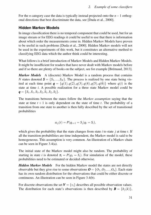
What follows is a brief introduction of Markov Models and Hidden Markov Models.It might be insufficient for readers that have never dealt with Markov models beforeand if so there are plenty of books on the subject, see for example [Brémaud, 2013].
Markov Models A (discrete) Markov Model is a random process that containsN states denoted SSS = {S1, ...,SN}. The process is realized by one state being vis-ited at each time point qqq = {q(1),q(2),q(3),q(4),q(5),q(6)} where q(i) is thestate at time i. A possible realization for a three state Markov model could beqqq = {S1,S1,S3,S2,S1,S2,S2}.
The transitions between the states follow the Markov assumption saying that thestate at time t + 1 is only dependent on the state of time t. The probability of atransition from one state to another is then fully described by the set of transitionalprobabilities
ai j(t) = P(qt+1 = S j|qt = Si),
which gives the probability that the state changes from state i to state j at time t. Ifall the transition probabilities are time independent, the Markov model is said to behomogeneous. This assumption is very common. An illustration of a Markov chaincan be seen in Figure 3.4(a).
The initial state of the Markov model might also be random. The probability ofstarting in state i is denoted πi = P(q1 = Si). For simulation of the model, theseprobabilities need to be estimated or decided otherwise.
Hidden Markov Models For the hidden Markov model the states are not directlyobservable but they give rise to some observations OOO = {O1,O2, ...,On}. Each statehas its own random distribution for the observations that could be either discrete orcontinuous. An illustration can be seen in Figure 3.4(b).
For discrete observations the set VVV = {vi} describes all possible observation values.The distribution for each state’s observations is then described by BBB = {b j(k)},
31

Chapter 3. Classification
S1
S2 S3
a11
a12 a13
a22
a21
a23a33
a31
a32
(a) Markov Model
S1 S2
vvv111 vvv222
a11
a12
b1(1)
b1(2)
a22a21
b2(1)
b2(2)
(b) Hidden Markov Model
Figure 3.4 (a) Example of Markov model, (b) Example of hidden Markov model. Thestates Si are not directly observable, but we can see the observations vi.
where b j(k) = P(vk at time t|qt = S j).
To summarize, the following is needed to design a hidden Markov model with dis-crete observation space.
1. The number of states N.
2. The possible observations V = {vi}.
3. The transition probabilities A = {ai j}.
4. The distribution of the observations B = {b j(k)}.
5. The initial distribution πi = P(q1 = Si).
There are three problems that need to be solved to use HMM for classification.Those will be presented, but the solutions see [Duda et al., 2000], [Juang and Ra-biner, 1991].
The evaluation problem: Given a model λ = (A,B,π) and a set of observations OOO,compute P(OOO|λ ) in an efficient way. This is the probability that the model generatedthe observations.
The decoding problem: Given a sequence of observations OOO and a model λ deter-mine the most probable set of states qqq.
The learning problem: Given a set of observation sequences {OOOi}, determine theset of parameters λ = (A,B,π) to maximize P(OOO|λ ).
32

3. Algorithm independent theory
S1 S2 S3
Figure 3.5 Example of a left right Markov model. Once a node has been left, it can not berevisited.
Example: Speech Recognition We now try to illustrate how we can build a clas-sifier using the solution to these problem by presenting an example from [Juang andRabiner, 1991].
Consider the classification of individual words. Assume that each word can be rep-resented as a time sequence of M unique spectral vectors. This is done by mappingeach time segment to the closest spectral vector. So for each word there is a se-quence of observations OOO. By using the solution to the learning problem a hiddenMarkov model can be built for each word.
By using the decoding problem it is possible to examine how good our model seemsto be and make adjustments to the number of states N.
Finally, the solution to the evaluation problem can be used to classify a new wordby calculating which model that was most likely to have generated the test word’sspectral vector. �
Different HMM For speech recognition it makes sense to allow the process toreturn to a node that has already been visited. But for some process it might bebeneficial to force the process to move forward by only allowing state transitions inone direction. This can be implemented with a so called left right model, see Figure3.5 . This has been used in BCI research [Obermaier et al., 2001].
3. Algorithm independent theory
IntroductionIn this section properties that are general for all machine learning algorithms arediscussed. The two interesting theoretical questions "Is there an inherently strongerclassifier" and "Is there a best feature representation?" are answered. Next, general-ization performance is studied using the concepts of overfitting and underfitting.
Superior ClassifierNo Free Lunch theorem As stated in the introduction the goal is to get good gen-eralization performance. An interesting question is if there is any classifier that can
33
Chapter 3. Classification
be considered generally superior, or if there even is one that is superior to chance.The answer to this question is given by the No Free Lunch Theorem and it statesthat in the absences of assumptions all classifiers are expeced to have the sameperformance. For a formal statement of it see [Duda et al., 2000].
Ugly Duckling theorem So there is no reason to lean towards any classifier be-fore the problem is taken into account. What about the choice of features? Theanswer is given by the Ugly Duckling theorem, which states “There is no problem-independent or "best" set of features or feature attributes” [Duda et al., 2000].
Note that the implication of this theorem is only that we can not choose a featureset before taking the problem into account.
Classifier ComplexityIn the introduction it was said that having a too complex classifier could lead to badtesting accuracy even though the training accuracy was good. This is often calledoverfitting and can be simplified as having two different sources [Hawkins, 2004]:
• Using a model that is more advanced than it need to be. For example, if thedata can be separated linearly it might do more harm than good to use aquadratic decision surface.
• Using irrelevant or too many features.
The first part can be counteracted when designing the classifier and the second partis counteracted during feature selection. It is, however, important that the featureselection is adapted to the classifier that is later going to be used.
Due to the No Free Lunch theorem no classifier, including a simpler one, can beexpected to be better before taking the problem into account. Focusing too much onavoiding overfitting could lead to underfitting, which means both bad training andtesting accuracy. This can be explained by
• Using a model that is too simple
• Using too few features.
Clearly, avoiding overfitting might lead to underfitting and vice versa. This will beformalized with the help of the bias-variance tradeoff in the following paragraphs.
34

3. Algorithm independent theory
Bias and variance for regression Even though the rest of the report does not dealwith regression it will be used here since it is a clear illustration of the bias andvariance for a classifier.
The goal of regression is to estimate the function F(xxx) : Rn → R with the help oftraining data D = {(xxxi,y)}. This gives the regression function g(xxx;D) : Rn → R
which is the estimation of F(xxx). The effectiveness of the regressor could be mea-sured by its mean squared error averaged over all possible training data sets D .
ED [(g(xxx;D)−F(xxx))2] = (ED [g(xxx;D)−F(xxx)])2︸ ︷︷ ︸bias2
+ED
[(g(xxx;D)−ED [g(xxx;D)])2
]︸ ︷︷ ︸
variance(3.12)
It is noticed that the expected error has two terms, the bias and the variance. Thebias is how far off it is expected to be on average. It should be intuitively clear thathigher bias leads to lower accuracy without looking at the formula above. Variancemeasures how much the accuracy of the guess varies. Clearly a large variation inaccuracy means that the total accuracy suffers.
Now all that has to be done is to lower the bias and variance. The problem is thatonce a model has been chosen it is hard to decrease them both at the same time.Making the model more complex will lead to lower bias but higher variance. Whilemaking it less complex will lead to lower variance, but higher bias. In the poly-nomial fitting example earlier the first degree polynomial has some bias and lowvariance while the fourth degree polynomial has zero bias, since over any trainingset the error will be zero, but high variance.
With this in mind the design of a classifier could be seen as a two step process.First a classifier model has to be chosen. It is important to chose one that fits theproblem well to reduce the bias and variance. One can also try to get as manytraining samples as possible to further reduce bias and variance. The second step isfinding the optimal complexity for the model which gives the best combination ofbias and variance, i.e., the best compromise between over- and underfitting.
If one, for example, chooses a hidden Markov model with sufficiently many states,all training samples can be classified correctly but test performance will most likelybe bad. If one instead chooses too few states the model will perform badly both intraining and in testing.
See Figure 3.6 for an illustration of the concept.
For classification the error is instead a product of the bias and the variance [Dudaet al., 2000], but the same principles still apply.
35

Chapter 3. Classification
Figure 3.6 Illustration of the bias variance trade-off. A too simple model leads to bad train-ing and test accuracy. Using a too complex model will give good training accuracy, but badtest accuracy as the model finds all the patterns in the training set instead of the general pat-terns. The goal of the designer should be to find the complexity that maximizes test accuracy.
4. Support Vector Machines
A support vector machine (SVM) uses a linear decision boundary to classify newsamples. The training samples are for now assumed to be linearly separable and thecase for which they are not will be handled later. There are typically many linesthat separate the data, see Figure 3.7. The idea of SVM is to choose the decisionboundary that maximizes the margin of the training data in the sense that the min-imum margin is maximized. The minimum margin is the distance to the decisionboundary of the samples closest to it. The reasoning being that this will hopefullymaximize the chance for new data to be correctly classified.
A new sample~xi can be classified according to
if ~w ·~xi +b≥ 0 then positive, otherwise negative. (3.13)
So the orientation of line ~w and the bias b must be found. For the training samplesit is required that
36
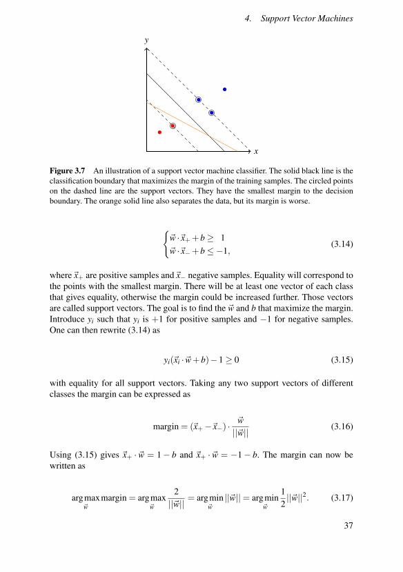
4. Support Vector Machines
y
x
Figure 3.7 An illustration of a support vector machine classifier. The solid black line is theclassification boundary that maximizes the margin of the training samples. The circled pointson the dashed line are the support vectors. They have the smallest margin to the decisionboundary. The orange solid line also separates the data, but its margin is worse.
{~w ·~x++b≥ 1~w ·~x−+b≤−1,
(3.14)
where~x+ are positive samples and~x− negative samples. Equality will correspond tothe points with the smallest margin. There will be at least one vector of each classthat gives equality, otherwise the margin could be increased further. Those vectorsare called support vectors. The goal is to find the ~w and b that maximize the margin.Introduce yi such that yi is +1 for positive samples and −1 for negative samples.One can then rewrite (3.14) as
yi(~xi ·~w+b)−1≥ 0 (3.15)
with equality for all support vectors. Taking any two support vectors of differentclasses the margin can be expressed as
margin = (~x+−~x−) ·~w||~w||
(3.16)
Using (3.15) gives ~x+ · ~w = 1− b and ~x+ · ~w = −1− b. The margin can now bewritten as
argmax~w
margin = argmax~w
2||~w||
= argmin~w||~w||= argmin
~w
12||~w||2. (3.17)
37
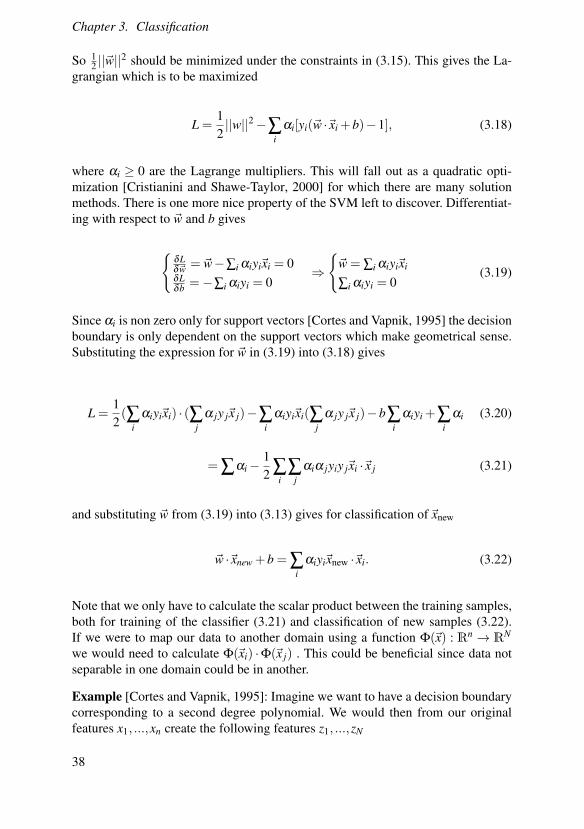
Chapter 3. Classification
So 12 ||~w||
2 should be minimized under the constraints in (3.15). This gives the La-grangian which is to be maximized
L =12||w||2−∑
iαi[yi(~w ·~xi +b)−1], (3.18)
where αi ≥ 0 are the Lagrange multipliers. This will fall out as a quadratic opti-mization [Cristianini and Shawe-Taylor, 2000] for which there are many solutionmethods. There is one more nice property of the SVM left to discover. Differentiat-ing with respect to ~w and b gives
{δLδ~w = ~w−∑i αiyi~xi = 0δLδb =−∑i αiyi = 0
⇒
{~w = ∑i αiyi~xi
∑i αiyi = 0(3.19)
Since αi is non zero only for support vectors [Cortes and Vapnik, 1995] the decisionboundary is only dependent on the support vectors which make geometrical sense.Substituting the expression for ~w in (3.19) into (3.18) gives
L =12(∑
iαiyi~xi) · (∑
jα jy j~x j)−∑
iαiyi~xi(∑
jα jy j~x j)−b∑
iαiyi +∑
iαi (3.20)
= ∑αi−12 ∑
i∑
jαiα jyiy j~xi ·~x j (3.21)
and substituting ~w from (3.19) into (3.13) gives for classification of~xnew
~w ·~xnew +b = ∑i
αiyi~xnew ·~xi. (3.22)
Note that we only have to calculate the scalar product between the training samples,both for training of the classifier (3.21) and classification of new samples (3.22).If we were to map our data to another domain using a function Φ(~x) : Rn → RN
we would need to calculate Φ(~xi) ·Φ(~x j) . This could be beneficial since data notseparable in one domain could be in another.
Example [Cortes and Vapnik, 1995]: Imagine we want to have a decision boundarycorresponding to a second degree polynomial. We would then from our originalfeatures x1, ...,xn create the following features z1, ...,zN
38

4. Support Vector Machines
z1 = x1, ..., zn = xn : n dimensionszn+1 = x2
1, ..., z2n = x2n : n dimensions
z2n+1 = x1x2, ..., zN = xnxn−1 : n(n−1)2 dimensions
We can see that for a second order polynomial the dimensionality of the new space ismuch larger than the original one. Calculating Φ(~xi) ·Φ(~x j)=~zi ·~z j could potentiallytake very long time. This can be avoided by the kernel trick. �
The idea is to replace Φ(~xi) ·Φ(~x j) with a kernel function K(~xi,~x j) that never has tomap the data to the higher dimensional space. There is some Hilbert space theoryfor when this is possible. Details will not be covered, but one theorem used laterwill be stated.
Theorem: Mercer Condition [Cortes and Vapnik, 1995]. A necessary and suffi-cient condition for that K(uuu,vvv) defines a dot-product in a feature space is that
∫ ∫K(uuu,vvv)g(uuu)g(vvv) duuudvvv≥ 0 (3.23)
for all g such that
∫g2(uuu) duuu < ∞. (3.24)
�
For a polynomial of degree d it is known that K(~xi,~x j) = (~xi ·~x j +1)d can be used[Cortes and Vapnik, 1995]. This is much more efficient than mapping the vectorsfirst and then calculating the scalar product.
Radial basis function (RBF) uses the following kernel
K(uuu,vvv) = exp(−γ|uuu− vvv|2
), (3.25)
which gives desicions on the form [Cortes and Vapnik, 1995]
f (xxx) = sign
(n
∑i=1
αi exp{γ|x− xi|2}
)(3.26)
If γ is chosen big enough 100% training accuracy can be achieved as only localinformation is then used. Smaller γ will mean that more points are used and the
39

Chapter 3. Classification
Figure 3.8 An illustration of a decision boundary for a radial basis function kernel. A lineardecision boundary is found in the kernel space which then maps to a non linear boundary inthe original space.
decision boundary will be less complex. An illustration of a decision boundary froman RBF kernel can be seen in Figure 3.8.
The benefits of SVM is that it guarantees finding a global minimum and that it canefficiently map the data to a higher dimension without paying with much highercomputation time. So far it was assumed that the data is linearly separable, at leastin some domain. Being restricted to finding a domain where the data is linearlyseparable would make the method useless for most cases. Luckily this can be coun-teracted.
Non separable caseFor the non separable case we require that
{yi(~xi ·~w+b)≥ 1−ξi
ξi ≥ 0(3.27)
This allows for some of the samples to be on the other side of the margin or even onthe other side of the decision boundary. ξi is the distance from the margin. We thenminimize
40
4. Support Vector Machines
min12||~w||2 +C∑
iξ
ki . (3.28)
We notice that choosing a large regularization parameter C will lead to fewer train-ing errors but possibly lead to overfitting since training errors are heaviliy penalized.The standard choices of k is 1 or 2, leading to the 1-norm and 2-norm soft marginproblem. For the solution to those see [Cristianini and Shawe-Taylor, 2000]. It isclear that the 1-norm is less sensitive to outliers.
Even for the separable case it could be useful to allow for some samples to havesome error ξi to increase the margin. This could lead to lower training accuracy, butalso to higher validation accuracy.
Generalization PerformanceThe regularization parameter C gives the user good control with regards to over-fitting. For radial basis function the user have further control with the parameterγ .
SVM have good generalization properties and are insensitive to overtraining [Lotteet al., 2007]. The complexity of a SVM is based on the decision boundary and notthe number of features [Joachims, 1998]. Hence for a linear kernel many featurescan be used while still keeping a low complexity kernel. Using a non linear ker-nel makes the model more complex and makes overfitting an issue that must beconsidered.
SVM multiclass classificationThe observant reader might have noticed that SVMs can only classify between twoclasses. There are two standard methods to extended the SVM framework to multi-class problem.
one against one In one vs one classification, each class is paired with all the otherclasses. The final result is the class that wins the most duels. Ties can be broken aslong as the same features are used for all classifiers.
one against all In one vs rest each class is instead fed into a classifier problemwere the competing class consists of all other classes. Hopefully only one classwins against the rest, but if multiple do, the resulting tie can be broken.
See [Hsu and Lin, 2002] for further treatment.
41

Chapter 3. Classification
0 1 2 3 4 5 6−1
−0.5
0
0.5
1
Figure 3.9 An example of how the Euclidean norm might be insufficient to compare timeseries. The black seesaw signal is closer to the green sinusoid than the red delayed sinusoidis. If one wants to decide if the given signal is a sinusoid or a seesaw signal the time shift isirrelevant.
5. Time Series Classification using SVM
It is possible to classify time series with SVMs using the theory covered so far byusing each data point from the time series as a feature. This could, however, be un-satisfying since the time dynamics are not taken into account. If all time points wereshuffled randomly (same for all samples) the classification would work out exactlythe same. Clearly some information is lost in the shuffling, but it is important to re-member that adding explicit time series is not guaranteeing improved performance.
This work will extend SVM to allow for classification of time series via dynamictime warping (DTW) which will be covered next.
Dynamic Time WarpingThere are many ways of measuring the similarity of two time series xxx = {xi} andyyy= {yi}. One might be tempted to use the L2 norm |xxx−yyy|. This simple approach hassome problems. Two identical signals with just one sample delay could be measuredas very different. An illustration of this can be seen in Figure 3.9.
The idea of dynamic time warping is to counteract time shifts and change in timescale by finding the alignment of the signals that has the lowest distance. This isdone by defining a warping between the first xxx = (x1,x2, ...,xN) and the secondsignal yyy = (y1,y2, ...,yN). The warping is defined by the warping sequence ppp =
42

5. Time Series Classification using SVM
(a) Valid Path (b) Invalid Path
Figure 3.10 (a) shows an illustration of a valid warping. (b) shows an invalid warpingwhere the invalid paths are marked red. The first one takes a too long step and the second onedoes not satisfy the monotonicity condition.
(p1, p2, ..., pL) where pl = (nl ,ml) means that xnl and yml should be compared. Thewarping path must satisfy the following [“Dynamic Time Warping” 2007]
1. The boundary conditions states that p1 = (1,1) and pn = (N,N).
2. Monotonicity condition n1 ≤ n2 ≤ ...≤ nn and m1 ≤ m2 ≤ ...≤ mn.
3. Step size pl+1− pl ∈ {(1,0),(0,1),(1,1)}.
An illustration of a valid path and an invalid path can be seen in Figure 3.10. Notethat a warping path might contain more comparisons than the L2 norm. The cost fora path is then calculated as
cp(xxx,yyy) =L
∑l=1
c(xnl ,yml ). (3.29)
The distance between two sequences is then chosen as one of the potentially multi-ple minimum paths. Now, only the question of finding the optimum path p is left.Calculating all possible paths would be very slow. This problem is solved by dy-namic programming, which allows the calculation to be done in O(N2) time com-plexity.
Multivariate DTW To reach good classifier performance it would be beneficial touse multiple time series. The two simplest ways to handle this would be to eitherwarp them independently or force them to all have the same warp.
43
Chapter 3. Classification
Normalization Normalizing each time point independently of the other timepoints would defeat some of the purpose of the time warping. One possible nor-malization is to normalize the time series, but then scaling information would belost.
Using DTW In Support Vector MachinesWith the theory covered so far it would be possible to design a k-nearest neighborclassifier using dynamic time warping as the distance measure. There is still somework to be done to use it in a support vector machine.
One might be tempted to define a kernel as k(xxx,yyy) = −DDTW (xxx,yyy) but this is nota valid Kernel [Gudmundsson et al., 2008]. Neither is the gaussian kernel attemptk(xxx,yyy) = exp
(−DDTW (xxx,yyy)
σ2
)[Lei and Sun, 2007]. The problem is that they are not
positive semidefinite which means they do not satisfy the Mercer condition, statedin (3.23). This means that the optimization problem is no longer convex. While it isstill possible to find a separating hyperplane we can not be sure that it is the optimalone. Cuturi [Cuturi, 2011] solved this by introducing the Fast Global alignmentkernel.
This work will use the pairwise proximity function SVM formulated by [Gud-mundsson et al., 2008]. This method relies on a proximity function instead of akernel function. Let X be the feature space, then P : X×X 7→ R maps each pair offeature vectors to their distance.
Given the training set {xxxi} define
φφφ(x) =(
P(xxx,xxx111),P(xxx,xxx222), ...,P(xxx,xxxnnn)). (3.30)
This function maps the features to a new feature space where each feature is thedistance to one of the training vectors. P will be the DTW distance and the SVMcan be trained using these features.
6. BCI classification
There are two ways to handle the time property of BCI signals. When classifying atime interval a static classifier just concatenates the features of different time pointsinto a feature vector for the whole time segment. Using this technique the informa-tion at each time point is used. However, the information that time point t1 comesbefore t2 is completely lost. This can be realized by concatenating the time vectorsin a different order. The classifier would work exactly the same!
44

6. BCI classification
A dynamic classifier instead classifies a sequence of feature vectors, like hiddenMarkov models classifiers. This is a common practice in speech recognition, butnot very used in BCI research.
In [Hwang et al., 2013] it was found that the dominant classifiers in BCI researchduring the period 2007-2011 was Linear Discriminant Analysis (36%) and supportvector machines with 17%. The rest were below 5 %.
A classifer for a BCI problem often needs to handle noisy high dimensional dataand few training sets.
45

4Feature Reduction
1. Introduction
MotivationIn some classification problems there is a lot of measurements that are candidatefeatures for classification. Reducing the amount of features fed into the classifier iscalled feature reduction. A perfect classifier would have no need for feature reduc-tion since it would be able to ignore irrelevant features. In practice no classifier isperfect but there is still no guarantee that we can improve its accuracy with featureselection. For EEG signals there are a lot of candidate features so it is likely thata good feature selection can improve the accuracy by removing irrelevant featuresand reducing overfitting.
The original feature input might also be so large that it has considerable impact onthe running speed, limiting real time performance. This further motivates the use offeature reduction.
OverviewFeature reduction can be split into two categories, feature selection where only someof the original features are kept and feature extraction where the original featurespace is transformed into one with lower dimension. Methods can further be splitinto supervised, where the labels of the training samples are known, and unsuper-vised where they are not known.
Feature selection is usually employed when there are many features to start with.This means that the time complexity of the algorithm is very important. An exhaus-tive search is generally not possible and one has to settle for a near optimal solution.This is usually implemented by searching the feature space by a heuristic or non de-terministic approach and finding a useful criterion to evaluate the current solutioncandidate. Heuristic approaches tend to get stuck in local extrema, while non deter-
46

2. ANOVA
ministic approaches need to be run multiple times as the results can differ betweenruns due to its random nature.
The feature selection is done offline so while it is important to keep the speed rea-sonably fast, it does not impact the run speed.
The two standard evaluation categories are wrapper methods and filter methods.Wrapper methods is the intuitive choice since they use the classifier accuracy asa metric. However, when an advanced classifier is used, the time it takes to trainthe classifier for each feature set to be tested might be impractical. Filter methodsevaluate the feature set with some other measure. It can for example use correlationor uncertainty measures from information theory [Huang, 2015].
One example of an heuristic seach apporach is Forward Selection. It starts with anempty feature set and adds the feature that improves the evaluation function themost. This contintues until a certain number of features have been added or thereare no features that improves the evaluation function [Rejer and Lorenz, 2013].Backwards selection instead starts with all features and removes the feature that isbest to remove one at a time. Forward and backward selection can be combined sothat features are first added and then removed.
2. ANOVA
Analysis of variance (ANOVA) is often used when evaluating results of experimentswhere different parameters are tested [Penny et al., 2011]. This work will use one-way ANOVA, which tests the hypothesis that the means of different classes are thesame. This hypothesis is discarded on a confidence level α when there is a 1−α
chance that the means are all not the same. So the chance that the hypothesis waswrongfully discarded is α . It can also be used as a feature selection method by onlychoosing features where the means are not all the same.
The data is assumed to be normally distributed for ANOVA. This is generally nottrue for the EEG data. This does not mean that the tests are useless. A high confi-dence level will still be a good indication that the means are not all the same.
ANOVA could be seen as a filter method, where the feature set is decided by eachfeature being evaluated individually using the ANOVA test described above.
When there are only two classes present, a T-test is sufficient to decide if the meansare the same. One-way ANOVA is a generalization of this, so the theory for a T-testwill be presented first.
47

Chapter 4. Feature Reduction
T-testFor a T-test, the data is assumed to be drawn from two different distributions Xi ∈N(µi,σi). There are two competing hypotheses
{H0 : µ1 = µ2
H1 : µ1 6= µ2(4.1)
Using the measurements xi1 and xi
2 the test quantity T can be calculated
T =x1− x2√
s21/N1 + s2
2/N2
(4.2)
where xi is the sample mean, s2i sample variance and Ni the number of samples of
each class. The zero hypothesis H0 is discarded on significance level α if |T | >t1−α/2. Or put in other words, H1 is said to be true with probability 1−α .
One-Way ANOVAOne-way ANOVA tests the hypothesis that all means are the same versus the hy-pothesis that they are not all the same. So to be clear, it is enough that two meansare different.
Since only the three class case will be used in this work the presentation of ANOVAwill only use three classes. This is easily generalized to n classes.
Let the means be described by β1, β2, β3 and the number of samples for each classby N1, N2, N3. The samples are then assumed to be given by
yi j = βi + ei j (i = 1, ...,3; j = 1, ...,Ni) (4.3)
Where {ei j} is independent and N(0,σ2) distributed. Then two quantities are cal-culated
SSbetween =3
∑i=1
Ni(yi− y)2 (4.4)
SSwithin =3
∑i=1
Ni
∑j=1
(yi j− yi)2 (4.5)
48
3. Correlation-Based Feature Selection
where y is the sample mean for all samples and yi is the sample mean for all thesamples in class i. SSbetween is a measure of the spread between the means of theclasses. SSwithin is a measure of the spread within the classes.
The test quantity for I classes is F = MSbetween/MSwithin, where
MSbetween = SSbetween/(I−1) MSwithin = SSwithin/(n− I) (4.6)
where n is the total number of samples. The hypothesis that all the means are equalare rejected at significance level α , by a comparison with the F distribution, if andonly if F > Fα;I−1,n−I . For a rigorous treatment see for example [Scheffé, 1959].
3. Correlation-Based Feature Selection
In the general sense two things are said to be correlated if knowing something aboutone tells you something about the other. Clearly one wants features that are corre-lated with the classes so that the value of the features can be used to make predictionabout the classes.
Correlation-based feature selection is a method for feature selection developed byHall [Hall, 1998]. It is based on the following principle
"Good feature subsets contain features highly correlated with the class, yet uncor-related with each other."
The idea is that having features that are correlated adds very little information, whileincreasing the risk of overfitting.
To penalize correlated features a feature subset S is evaluated by calculating
MS =krc f√
k+ k(k−1)r f f. (4.7)
Where k is the number of features in the subset, rc f is the average class-featurecorrelation and r f f is the average feature-feature correlation. A high feature-classcorrelation and a low feature-feature correlation is wanted. So a larger value of MS
is better.
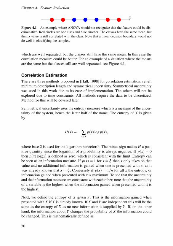
One might then ask what the point is of using correlation for feature selection.Or rather in what scenarios it outperforms ANOVA. For features that separate theclasses into two groups, ANOVA will do a good job since their means will be differ-ent. There could however be features that separate the samples into multiple groups
49
Chapter 4. Feature Reduction
x
Figure 4.1 An example where ANOVA would not recognize that the feature could be dis-criminative. Red circles are one class and blue another. The classes have the same mean, buttheir x value is still correlated with the class. Note that a linear decision boundary would notdo well in classifying the samples.
which are well separated, but the classes still have the same mean. In this case thecorrelation measure could be better. For an example of a situation where the meansare the same but the classes still are well separated, see Figure 4.1.
Correlation EstimationThere are three methods proposed in [Hall, 1998] for correlation estimation: relief,minimum description length and symmetrical uncertainty. Symmetrical uncertaintywas used in this work due to its ease of implementation. The others will not beexplored due to time constraints. All methods require the data to be discretized.Method for this will be covered later.
Symmetrical uncertainty uses the entropy measure which is a measure of the uncer-tainty of the system, hence the latter half of the name. The entropy of X is givenby
H(x) =−∑x∈X
p(x) log p(x),
where base 2 is used for the logarithm henceforth. The minus sign makes H a pos-itive quantity since the logarithm of a probability is always negative. If p(x) = 0then p(x) log(x) is defined as zero, which is consistent with the limit. Entropy canbe seen as an information measure. If p(x) = 1 for x = ξ then x only takes on thatvalue and no additional information is gained when one is presented with x, as itwas already known that x = ξ . Conversely if p(x) = 1/n for all x the entropy, orinformation gained when presented with x is maximum. To see that the uncertaintyand the information measure are consistent with each other, note that the uncertaintyof a variable is the highest when the information gained when presented with it isthe highest.
Next, we define the entropy of X given Y . This is the information gained whenpresented with X if Y is already known. If X and Y are independent this will be thesame as the entropy of X as no new information is supplied by Y . If, on the otherhand, the information about Y changes the probability of X the information couldbe changed. This is mathematically defined as
50

3. Correlation-Based Feature Selection
H(X |Y ) =−∑y∈Y
p(y) ∑x∈X
p(x|y) log p(x|y)
There are two cases. One where Y is another feature in which case the conditionalprobability can be written as
p(x|y) = p(x,y)p(y)
.
Clearly the distribution of a good feature will change when the class is known.
The other case is when Y is one of the classes. Then the conditional probabilitieswill easily be calculated as the probabilities for the features of the samples withinthat class.
If the entropy for X decreases when Y is supplied then additional information wasgained. Define this gain, also called mutual information, as
gain = H(X)−H(X |Y )= H(Y )−H(Y |X)
= H(Y )+H(X)−H(X ,Y ),(4.9)
where it is noticed that the last form can be used for calculation. Normalization canbe done so that the gains are comparable for different features via
symmetrical uncertainty coefficient = 2 ·[
gainH(X)+H(Y )
].
The factor two makes the range to be [0,1].
DiscretizationTwo simple methods for discretization is equal interval width and equal frequencyintervals. Equal interval width splits the data into n bins where each bin covers aninterval of size l so that all features are covered. Equal frequency interval splits thedata into n bins where each bin contains the same amount of data points.
There are more advanced methods. One based on minimum description will bebriefly introduced below. For a full treatment see the original article [Fayyad, 1993].
51
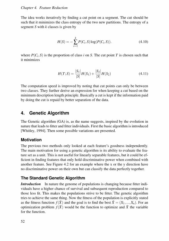
Chapter 4. Feature Reduction
The idea works iteratively by finding a cut point on a segment. The cut should besuch that it minimizes the class entropy of the two new partitions. The entropy of asegment S with k classes is given by
H(S) =−k
∑i=1
P(Ci,S) log(P(Ci,S)). (4.10)
where P(Ci,S) is the proportion of class i on S. The cut point T is chosen such thatit minimizes
H(T ;S) =|S1||S|
H(S1)+|S2||S|
H(S2) (4.11)
The computation speed is improved by noting that cut points can only be betweentwo classes. They further derive an expression for when keeping a cut based on theminimum description length principle. Basically a cut is kept if the information paidby doing the cut is repaid by better separation of the data.
4. Genetic Algorithm
The Genetic algorithm (GA) is, as the name suggests, inspired by the evolution innature that leads to fitter and fitter individuals. First the basic algorithm is introduced[Whitley, 1994]. Then some possible variations are presented.
MotivationThe previous two methods only looked at each feature’s goodness independently.The main motivation for using a genetic algorithm is its ability to evaluate the fea-ture set as a unit. This is not useful for linearly separable features, but it could be ef-ficient in finding features that only hold discriminative power when combined withanother feature. See Figure 4.2 for an example where the x or the y direction haveno discriminative power on their own but can classify the data perfectly together.
The Standard Genetic AlgorithmIntroduction In nature the genome of populations is changing because fitter indi-viduals have a higher chance of survival and subsequent reproduction compared tothose less fit. This makes the populations strive to be fitter. The genetic algorithmtries to achieve the same thing. Now the fitness of the population is explicitly statedas the fitness function f (X) and the goal is to find the best X = (X1, ...,Xn). For anoptimization problem f (X) would be the function to optimize and X the variablefor the function.
52

4. Genetic Algorithm
−1 −0.8 −0.6 −0.4 −0.2 0 0.2 0.4 0.6 0.8 1−1
−0.8
−0.6
−0.4
−0.2
0
0.2
0.4
0.6
0.8
1
Figure 4.2 An example where the two features have no disciminative power on thier own,but do together. The blue circles and red crosses are the two different classes and the featuresare the x and y coordinates. Note that no linear decision boundary can do better than chance.
In this work GA will be used for feature selection where the number of featuresto be chosen are predetermined. The goal is to choose the n best features from thefeature candidates numbered 1, ...,N. The variable Xi can take on values in the range[1,N] to represent the feature chosen, but duplicates are not allowed.
If the size of the feature subsets is allowed to change then the encoding need to bebinary and X = (X1, ...,XN) and Xi = 1 encodes that feature i is present and Xi = 0that it is not.
The fitness function will measure the goodness of the feature subset. When classifierperformance is used the method is a wrapper method. It is also possible to use someother measure, making it a filter method.
The algorithm The algorithm is initialized with a genome of individuals. Eachindividual consists of a vector that encodes that individual’s vector X , This vectoris often called a chromosome.
The algorithm then iterates by evolving the genome. The first step to this is calcu-lating the evaluation function which is an absolute measure of how good the currentchromosome is, for example the value of f (X) or the accuracy of a classifier. Next
53

Chapter 4. Feature Reduction
the fitness function is calculated which is the chromosomes relative strength com-pared to the rest of the genome. This can for example be calculated as fi/ f wherefi is the evaluation function of the chromosome and f is the mean value of all theevaluation function.
The chromosomes next go through the selection process, which yields an interme-diate generation where a chromosome with a high fitness score might be presentmultiple time and one with a lower might not be present at all.
Next is the recombination step, where there is a chance that each chromosome iscombined with another chromosome generating two new offsprings. This is called acrossover and might, for example, be implemented by choosing a random crossoverpoint and splitting the chromosomes at that point and combining one half from each.
As a final step there is a small chance that an offspring goes through a mutationwhere one of its binary values will flip. This is the end of the iteration, and is fol-lowed by a new calculation of the fitness value. A graphical overview of the processcan be seen in Figure 4.3.
There are many possible stopping criteria. Examples include terminating after aspecific number of iterations, when the change in fitness is below a threshold orwhen the maximum fitness is above a threshold.
Overfitting in GA When using the wrapper GA there will be a set of samples wecan use for training and evaluation. There is a risk that the resulting classifier getsvery well-tuned for the data that is presented to it. This is not overfitting in the strictsense that was talked about in classification but the term is extended to cover thiscase as well. The classical overfitting is still a potential problem if the size of thefeature subset is not prespecified. This can be counteracted by punishing genes withmany features [Duda et al., 2000].
The tuning problem can be counteracted by not presenting the same data to thefitness function for each generation so that the classifier learns the trends and notthe testing set. Liu and Khoshgoftaar [Liu and Khoshgoftaar, 2004] showed thatrandom sampling technique (RST) reduces overfitting. The usage of RST meansthat only a subset of the training set is used for each generation. Thus presentingdifferent patterns every time.
Why does it work?There are many different variations and parameter sets for GA and there are nostrong theoretical statements for why it works. Instead, we have to believe in theprevious results shown, for example in the BCI field [Rejer and Lorenz, 2013], andits good properties.
54

4. Genetic Algorithm
InitialPopulation
fitnessfunction
selection
Crossover& mutation
Population
fittestindividual
Figure 4.3 A graphical illustration of the genetic algorithm. First an initial population ischosen. Then the fitness value is calculated for each individual. This fitness value gives theprobability for each individual to survive the selection process. Those that survive the se-lection process goes through crossover where 2 genes are combined together and mutationwhere there is a probability that one feature might swap to another. The fittest individual isextracted when the algorithm terminates.
ExtensionsDiversity The diversity of a population in GA is a measure of how spread outthe genome is. Failing to maintain a diverse solution might mean that the featurespace is not adequately searched, while too high diversity could lead to very slowconvergence [D. Gupta, 2012].
One method of maintaining diversity of the population is to use a ranked spacewhere each individual is ranked both on fitness and diversity. The fitness function isthen calculated based on this rank. An overview of other methods can be found in[D. Gupta, 2012].
Elitism In nature the parents can not live on for ever but in GA they can. Allowingthe parents to fight with their cross-over children for survival into the next gener-ation means that a gene is never replaced with one that has worse fitness duringrecombination. This might rapidly increase convergence, but at the cost of lowerdiversity.
Parameter Control For the classic genetic algorithm the crossover rate and muta-tion rate are set to be constant. The genetic algorithm is a very dynamic process soit is reasonable to use dynamic parameters. It might, for example, be better to have
55

Chapter 4. Feature Reduction
higher mutations rate in the beginning to help explore the search space and lowermutation rate later to fine tune the solutions.
Parameter control can be classified as deterministic in which it changes determinis-tically for each generation, as adaptive where it changes depending on the propertiesof the entire population or and self adaptive where the parameters themselves areencoded in the genome and undergoes crossover and mutation. For a thorough rep-resentation see [Eiben et al., 1999].
56

5Experimental Setup
1. The Study
The data for this project was supplied by the Department of Psychology at LundUniversity. The experiment is motivated by their research in memory representation.A visualization of the setup can be seen in Figure 5.1.
The study was conducted in a Faraday cage at the department of Psychology atLund University. The subjects were Swedish native speakers without any knownneurological or psychiatric disorders. Both males and females were participating.
The stimuli material of the study was 64 different pictures from the three categories"familiar faces", "landmarks" and "objects", yielding 192 pictures in total. The studywas split up into three parts. The first part was the familiarity task where the partic-ipant is shown a picture on a computer screen for a couple of seconds. The pictureswere taken from one of the three categories. The participants were then asked howwell it represents the concept of the picture. This could in theory be used to removepictures that were not recognized by participants, but was not used in practice.
The second part was the study phase for which 24 word-picture pairs were pre-sented and the participants was asked to try to remember the pair and also rate theassociation between the pair.
Finally for the test phase the participant was shown a word and needed to retrievethe category of the picture it was associated with. If they were correct they werethen also shown the original and a mirrored picture and had to choose which onethey thought they saw earlier. This was to force the participants to visualize thepicture, otherwise the retrieval is only conceptual. The goal of this was to increasethe classifier accuracy.
The study took approximately two and a half hour with breaks between each part.
The goal of the study at the psychology department was to study if any of the pat-
57

Chapter 5. Experimental Setup
Figure 5.1 Illustration of the experiment from which the data of this work originates. Thestudy consisted of three phases. During the familiarity phase the participants were showedpictures from three categories:faces, objects, and landmarks. During the study phase theywere asked to memorize word/picture pairs. For the test part the participants were tasked withremembering the picture that corresponded to the displayed word. Only the study phased wasused in this work. [Image source Inês Bramão Department of Psychology Lund University.]
terns during the encoding of the study phase were replayed during the recollectionof the test phase.
58
2. Classification Setup
The dataEEG was measured throughout the entire experiments with a frequency of 2048 Hz.This high frequency was used since it was necessary to detect triggers that weresent each time the picture changed. The data was later down-sampled to 512 Hz.The average of the left and the right mastoid is used as a reference for the data. Thatmeans that all other measurements are relative to the reference.
For each part one EEG segment was saved. For the familiarity part data was savedfor the display of the picture. For the study part the data was also saved for thedisplay of the picture. Finally, for the test part data was saved for the display of theword.
Data was saved from 1 second before the stimuli and up to 2.5 second after thestimuli. The reason for saving data before the stimuli and for so long after was toallow for frequency calculations. One such segment is called a trial.
Artifacts coming from sources such as eye and muscle movement were removedusing independent component analysis and the expertise at the psychology depart-ment. The removal of eye artifacts was also helped by measurements from VEOGand HEOG channels that measured vertical and horizontal eye movements. Trialsthat could not be cleaned up to a satisfactory degree were removed.
2. Classification Setup
FeaturesPower spectral density will be used as features throughout the experiments. Thedata to be classified will be split into time points. For each time point the magnitudeof a set of frequencies will be calculated. The phase of the signal will not be used.This will be done for each channel yielding a three dimensional space to choosefeatures from, see Figure 5.2 for a visualization.
For a static classifier, features can be chosen arbitrarily over this three dimensionalgrid. One might for example choose channel four, frequency magnitude at five Hzand time point four as a feature. If one instead wants to use a dynamic classifier thefeatures must instead be time series. An example of a feature is then channel four,frequency magnitude at five Hz and measurements from time point two to time pointeight.
Time binsThe goal of the study at the psychology department was to explore if part of theprocess of remembering (encoding) a memory was replayed during the retrieval ofthat memory. Those processes clearly will not be the same all the time. If one was
59

Chapter 5. Experimental Setup
Channelnumber
Time points
Frequency
Figure 5.2 Illustration of the possible features to choose from. For each channel the mag-nitude of some frequencies are calculated at different time points.
to build a classifier for the entire signal it would be impossible to tell at what timeeventual similarities happened.
To solve this, different classifiers are trained for different time intervals, called timebins. A time bin starts at t0 and ends at time t1 and uses only data from that timeperiod for training. The training data is split into time bins that cover the whole trial(could be overlapping). See Figure 5.3 for an illustration. All those time bins arethen used to classify the test phase. A classifier trained for a time bin that starts at t0and ends at t1 for the study data needs not to classify the same interval for the testdata. The interval it is run on needs, however, to have the same interval size.
The time bin technique is useful also in other BCI applications. Waiting for thewhole signal before doing any classification would however lead to systems withlarge delays. Daly et al [Daly et al., 2011] investigated the effect on accuracy fordifferent window sizes when identifying single taps. Smaller windows increase the
time bin 1 time bin 2 time bin 3
t1 t2 t3 t4 t5 t6 t7 t8 t9 t10 t11 t12
Figure 5.3 Illustration of the time bin concept. The samples are split into several indepen-dent time bins containing some of the samples each.
60

3. Previous Work
theoretical bit rate but at the cost of decreased accuracy.
The cited work also used sliding time windows. With this technique the output ofthe classifier can switch with every time point instead of the length of the timewindow, allowing the classification output to change more often without loss of ac-curacy. Sliding time bins require to use some information from prior time bins to beefficiently implemented, but in theory each time bin can be handled independentlyof other time bins.
3. Previous Work
Jafarpour et al. [Jafarpour et al., 2014] studied at what point in recollection theencoding of the memory was replayed. The study consisted of 3 phases. Duringthe first phase the participants were shown pictures of faces or scenes, which theyshould not have seen before. If they had, the picture was removed from the exper-iment. One classifier for faces and one for scenes were then trained from the datathat was kept.
For the second phase the participants were tasked with memorizing word-picturepairs. For the last phase the participants were shown a word and asked to try toremember the face/scene it was associated with. The classifier built was then usedduring the third phase with the idea being that a high classification score during atime slot meant that the original memory was replayed.
The machine learning used MEG readings from 274 channels. The data was thentransformed to the time frequency domain using 5 cycles Morlet wavelets (contin-uous wavelet transform). The frequency scale went from 8-45 Hz with a resolutionof 1 Hz. Analysis was performed in time bins of 66 ms and there were 21 timepoints in each time bin. Data was normalized by z-scoring (data normalized to zeromean and unite variance) at each time point, frequency and channel across trials. Asupport vector machine was the choice of classifier.
First they looked for category specific patterns during encoding. This was done byusing 10 fold cross validation. This means that for each time bin, 10 different clas-sifiers were trained. Each classifier uses a different 10 % of the data for validation.The accuracy was then the mean of the accuracy for the 10 classifiers. For eachvalidation pass a feature selection was run by only keeping those features that weresignificantly different between the two categories in a T -test with 0.05 level. Theperformance was then calculated as the average of all the 10 classifiers. The classi-fiers that were significantly different from zero were then trained on all the data intheir time bin.
These classifiers were then used to check if the pattern present during their timebin was later replayed during encoding which there were no indications of in the
61

Chapter 5. Experimental Setup
classifier performance.
They then checked if category specific patterns emerged during recollection. Thiswas done by running the classifier trained on data from the encoding time bin cen-tered around 180 ms on the recollection trials where the participants correctly rec-ognized the word cue. This gave significant classifier performance for the time binscentered at 446 and 513 ms. Sliding time bins were not used. This could possiblygive better performance as there is no guarantee that the replayed pattern is alignedwith one of the time bins.
Finally, only those recollection trials where the participants also chose the correctpicture were tested. Now the classifier was only significant for 513 ms.
62
6Method
1. Software
The matlab toolbox Fieldtrip toolbox [Oostenveld et al., 2011] was used in thiswork. It is developed by Donders Institute for Brain, Cognition and Behaviour inNijmegen, the Netherlands, and have multiple methods for analysis of EEG andMEG data. Methods for filtering the signals and to do time frequency calculationsusing continuous wavelets were used.
For SVM classification LIBSVM [Chang and Lin, 2011] was used. It is writtenin C++ and contains a Matlab interface. It supports one-vs-one multiclass SVMclassification.
2. Static Classifier
IntroductionThe goal of this part was to explore alternatives to the ANOVA + linear SVMmethod that was used by Jafarpour [Jafarpour et al., 2014] and by the psychologydepartment. It was decided to keep SVM as the classification method so the focuscould be kept on the feature selection. Other than ANOVA, two feature selectionmethods were tested: correlation based feature selection and genetic algorithm.
ExperimentAs the goal was to test which method performed best, it was important to have awell defined goodness measure. Time bins is a good tool for memory research, butit is hard to find a satisfying goodness measure for it. One could take the meanaccuracy over all time bins but it is not apparent that all time bins should be equallyimportant. It is yet unknown in what time segments good classifier performance isexpected from physiological reasons.
63

Chapter 6. Method
Signal Processing
Wavelet Transform
Feature Selection
Training Samples
•ANOVA•Genetic
•CFS
Classification
Training Samples
Support Vector Machine
EEG {time, freq} features Output
Figure 6.1 Illustration of the classification pipeline used in this project. The EEG signalsare first transformed using wavelet transform. Then features are chosen from the possiblecombination of time and frequency measurements. Those features are fed into a classifierthat outputs the prediction of the category for the input.
It was decided that it was better to evaluate classifier performance by classifyingthe whole time segment at the same time. This could be seen as having one largetime bin. Different methods might be better at classifying different length of signals(more efficient at using less data) or more efficient at different parts of the data.However, this approach should serve well as a first evaluation method. If multiplemethods are close then further experiments should be conducted.
The classification pipeline of this work have three steps. The first is signal process-ing, where the original EEG signals are transformed into the frequency domain. Thesecond step is feature selection, where the best features were chosen. Those featuresare fed into the third step, which is classification. An illustration of the this can beseen in Figure 6.1.
Base feature set For all experiments in this work the base feature set was thefrequency magnitude given by continuous wavelet transform.
Comparison with other work Using all the data at the same time instead of work-ing with only a subset of it will mean that the accuracy will be at least as good asthe accuracy for the best time bin, and most likely better. This means that it is hardto compare the results with other studies. But since there are no other publishedresults on this study that would be impossible anyway. Instead the comparison willbe between the old method, ANOVA, and the new tested in this work.
Rejected methodsTwo simple methods were tested initially and rejected due to bad performance. Herefollows a short description of them
Principal Component Analysis Principal component analysis (PCA) finds the di-rections were the data has the highest variance, see [Duda et al., 2000]. PCA wasused to find the directions where the spectral features had the largest variance. Thesefeatures were then fed into a linear support vector machine. The initial results werenot good enough to continue perusing this method.
64

2. Static Classifier
This was not unexpected as there likely is large in-class variance in the data.
Linear Discriminant Analysis Linear discriminant analysis was used in a smiliarway as PCA, i.e. projecting data into some new directions.. The method only givestwo directions for the three class problem. This was not sufficient to achieve goodclassifier performance and was not further investigated.
ANOVAMethod The ANOVA method evaluates each feature independently and performsa one way ANOVA test (Chapter 4.2). There are then two alternatives, either the nmost significant features are kept, or all features significant on an α level.
Next the features are normalized using z-scoring, so that all have zero mean and unitvariance. This is important so that the SVM does not give higher weight to featureswith larger values.
For classification a linear SVM was used.
Motivation The usage of a linear kernel is motivated both theoretically and byexperiments.
The features chosen by ANOVA are different in means between at least two of thethree classes. So in that feature’s direction a linear separator should do a good job.In the other directions there is no information. If a non linear kernel was to be usedthe amount of features would have to be reduced significantly to avoid overfitting.There is no theoretical motivation to do so since there is no indication that thefeatures would be good in a non linear kernel.
By experiments it was found that the previous arguments indeed were correct.
Correlations-Based Feature SelectionThe correlation based feature selection (Chapter 4.3) was initially motivated bykeeping the number of features low, to reduce overfitting. This is not really neededfor linear SVMs, since they handle correlated features well. Furthermore the cal-culation for inter-feature correlation gets really slow when the time and frequencyresolution is high. Due to this, the denominator containing the inter-feature correla-tion term r f f of equation (4.7) was ignored when a linear kernel was used.
The data was z-scored and then discretized. Features were then chosen viacorrelation-based feature selection and fed into a SVM.
Genetic AlgorithmSee Chapter 4.4 for an introduction to genetic algorithms. The data was first z-scored. Then feature selection was done using a genetic algorithm. The fitness
65

Chapter 6. Method
function was the classifier performance for the target SVM. To avoid overfitting,the features in the test and training set was randomized.
3. Dynamic Classifier
The idea to use a dynamic classifier came along late into the project. However, itwas still decided to introduce the concept and make a quick experiment.
FeaturesFeature definition In this work a feature was a time series containing the mag-nitude of a frequency over a channel. It is possible to let each time series have itsown start and finish time. But to keep it simple for this initial experiment each timeseries was forced to start at time zero and end at time T . Time T was chosen byinspection in Figure 6.2 that shows where features that passed the ANOVA test onan α = 0.1 level.
So the feature space consisted of all combinations of frequencies and channels. Oneexample would be the time series for the frequency 5 Hz at channel ten.
Feature Selection For feature selection ANOVA tests were calculated for all timepoints, channels and frequencies. Then a time series was kept if q percent of thesamples had significant level above α .
ExperimentFor classification, pairwise distance function (introduced in Chapter 3.5) was used.Dynamic time warping was used as the distance metric with the distance as costfunctions. All features were forced to have the same warping. The total distancewas calculated using the L 1 norm over all channels.
The pairwise distance features were then fed into a linear SVM.
The result was compared with the ANOVA method choosing features from the samefeature set and another pair wise distance classifer that used the L 2 norm insteadof dynamic time warping for each channel, but the L 1 over the channels.
The goal was to see if this dynamic classifier could outperform the static and if thedynamic time warping was useful.
66

3. Dynamic Classifier
1020
3040
20
40
60
5
10
15
20
25
30
freqtimepoint
Channel
Figure 6.2 Features that passed the ANOVA test on an α = 0.1 level. It can be seen thatthere are more selected features for lower frequencies and earlier time points. Colors corre-spond to channels.
67

7Results
For all cases, 40 samples from each category was used for training. The remainingtrials was then used for testing. For subject 9 that was 24 faces, 22 objects and22 landmarks. One subject was chosen to reduce work.This particular subject waschosen since it gave the highest classification accuracy.
Frequency calculation was done using the function ft_freqanalysis in Field Triptoolbox using (Morlet) wavelet and cfg.width = 5. The rest of the settings werethe defaults.
1. Static Classifier
Frequency is used from 5 to 49 Hz and time from 0 to 1 second. The full timesegment was used as the classifier should be able to handle if the features are worseafter a certain time point. The choice of 49 Hz was used since there is a lot ofdisturbances of 50 Hz due to the power line. The lower limit was chosen as 5 Hz,since low frequencies have bad time resolution and would lead to high delays ifused in a real-time BCI systems.
ANOVAThe ANOVA method was initially tested for other kernels than the linear. Thoseresults were however around chance and are not presented. The results for a linearkernel are given in Table 7.1.
It was found that the best performance was achieved for a significance level ofα = 0.01.
Correlation-based feature selectionCorrelation-based feature selection was tested for two cases. For the linear ker-nel only class-feature correlation was used. For the non-linear kernels the feature-feature correlation was also used. Uniform discretization of the features was used
68
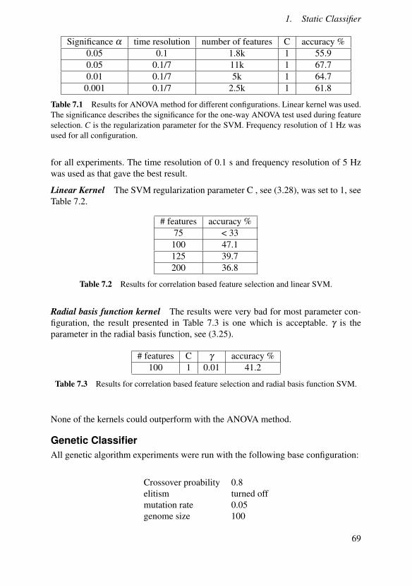
1. Static Classifier
Significance α time resolution number of features C accuracy %0.05 0.1 1.8k 1 55.90.05 0.1/7 11k 1 67.70.01 0.1/7 5k 1 64.7
0.001 0.1/7 2.5k 1 61.8
Table 7.1 Results for ANOVA method for different configurations. Linear kernel was used.The significance describes the significance for the one-way ANOVA test used during featureselection. C is the regularization parameter for the SVM. Frequency resolution of 1 Hz wasused for all configuration.
for all experiments. The time resolution of 0.1 s and frequency resolution of 5 Hzwas used as that gave the best result.
Linear Kernel The SVM regularization parameter C , see (3.28), was set to 1, seeTable 7.2.
# features accuracy %75 < 33100 47.1125 39.7200 36.8
Table 7.2 Results for correlation based feature selection and linear SVM.
Radial basis function kernel The results were very bad for most parameter con-figuration, the result presented in Table 7.3 is one which is acceptable. γ is theparameter in the radial basis function, see (3.25).
# features C γ accuracy %100 1 0.01 41.2
Table 7.3 Results for correlation based feature selection and radial basis function SVM.
None of the kernels could outperform with the ANOVA method.
Genetic ClassifierAll genetic algorithm experiments were run with the following base configuration:
Crossover proability 0.8elitism turned offmutation rate 0.05genome size 100
69
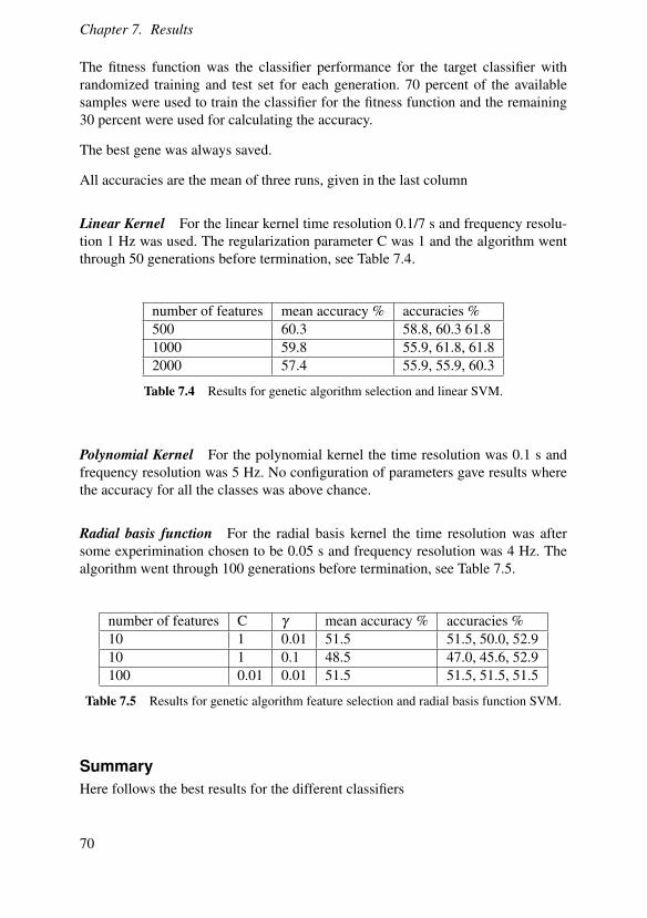
Chapter 7. Results
The fitness function was the classifier performance for the target classifier withrandomized training and test set for each generation. 70 percent of the availablesamples were used to train the classifier for the fitness function and the remaining30 percent were used for calculating the accuracy.
The best gene was always saved.
All accuracies are the mean of three runs, given in the last column
Linear Kernel For the linear kernel time resolution 0.1/7 s and frequency resolu-tion 1 Hz was used. The regularization parameter C was 1 and the algorithm wentthrough 50 generations before termination, see Table 7.4.
number of features mean accuracy % accuracies %500 60.3 58.8, 60.3 61.81000 59.8 55.9, 61.8, 61.82000 57.4 55.9, 55.9, 60.3
Table 7.4 Results for genetic algorithm selection and linear SVM.
Polynomial Kernel For the polynomial kernel the time resolution was 0.1 s andfrequency resolution was 5 Hz. No configuration of parameters gave results wherethe accuracy for all the classes was above chance.
Radial basis function For the radial basis kernel the time resolution was aftersome experimination chosen to be 0.05 s and frequency resolution was 4 Hz. Thealgorithm went through 100 generations before termination, see Table 7.5.
number of features C γ mean accuracy % accuracies %10 1 0.01 51.5 51.5, 50.0, 52.910 1 0.1 48.5 47.0, 45.6, 52.9100 0.01 0.01 51.5 51.5, 51.5, 51.5
Table 7.5 Results for genetic algorithm feature selection and radial basis function SVM.
SummaryHere follows the best results for the different classifiers
70
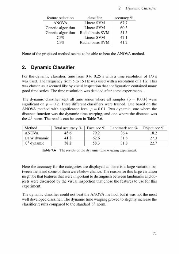
2. Dynamic Classifier
feature selection classifier accuracy %ANOVA Linear SVM 67.7
Genetic algorithm Linear SVM 60.3Genetic algorithm Radial basis SVM 51.5
CFS Linear SVM 47.1CFS Radial basis SVM 41.2
None of the proposed method seems to be able to beat the ANOVA method.
2. Dynamic Classifier
For the dynamic classifier, time from 0 to 0.25 s with a time resolution of 1/3 swas used. The frequency from 5 to 15 Hz was used with a resolution of 1 Hz. Thiswas chosen as it seemed like by visual inspection that configuration contained manygood time series. The time resolution was decided after some experiments.
The dynamic classifier kept all time series where all samples (q = 100%) weresignificant on p = 0.2. Three different classifiers were trained. One based on theANOVA method with significance level p = 0.01. Two dynamic, one where thedistance function was the dynamic time warping, and one where the distance wasthe L1 norm. The results can be seen in Table 7.6.
Method Total accuracy % Face acc % Landmark acc % Object acc %ANOVA 45.6 79.2 36.4 18.2DTW dynamic 41.2 62.6 31.8 27.3L1 dynamic 38.2 58.3 31.8 22.7
Table 7.6 The results of the dynamic time warping experiment.
Here the accuracy for the categories are displayed as there is a large variation be-tween them and some of them were below chance. The reason for this large variationmight be that features that were important to distinguish between landmarks and ob-jects were discarded by the visual inspection that chose the features to use for thisexperiment.
The dynamic classifier could not beat the ANOVA method, but it was not the mostwell developed classifier. The dynamic time warping proved to slightly increase theclassifier results compared to the standard L1 norm.
71
8Discussion andConclusions
1. Conclusions
The BCI technique is promising and is able to achieve high accuracy. However,so far no system manage to be both fast and accurate without having to focus ona stimuli. In addition, the gear is very immobile and sensitive. For industrial use,the speed of the systems must be increased, while atleast maintaining accuracy. Forindustrial use, the sensors needs to achieve a higher combination of portability andquality.
The results of the classifier on the data used could not be improved by the twofeature selection method tested.
The dynamic time warping experiment showed that there is some information to begained by using the time dynamics, however the magnitude of that information wasvery low for this particular dynamic classifier.
2. Discussion
For the experimental part of this work two things can be noted. Firstly, the geneticalgorithm had its best accuracy for fewer features than the ANOVA method forlinear kernel. That might be an indication that there is some overfitting problemin the configuration and implementation of the genetic algorithm. Even with thatsolved, it seems far fetched that it could beat the ANOVA method.
Secondly, the results for the non linear kernels were worse than the linear ones.Furthermore they had to use small γ so they were not that complex. It seems like itis best to use a linear kernel for the data set and the features used.
72

3. Future Work
3. Future Work
There are some techniques that could be explored in future work to improve theclassifier. Outlier rejection or sample weighting, where the error penalty dependson each samples could help deal with the possible noisy samples. Feature weight-ing could also be explored. At the moment all features are assumed to be equallyimportant as they are normalized the same way. Features could be normalized dif-ferently depending on how good they seem to be. This would allow for differentfeatures to have different impact.
It is the authors opinion that the dynamic classifier should be explored further. Thefirst thing to implement would be to allow each time series to start and end at dif-ferent times. Normalization of both time series and pair wise distance could be ex-plored. Another dynamic classifier could also be used, for example a hidden Markovmodel. Pair wise distance function SVM was used for its simplicity. Even if it is notsuperior on this data set it is expected to perform better in non-clinical applicationswere the signals are not as well aligned.
Features and classifier should be chosen with the problem in mind. But this workused simple features and a classifier that is known to do well with high dimensionaldata. Overall the approach have been of a somewhat black box nature. We havesome inputs coming from something and we want to classify them.
This was fine for this project as it tried to improve upon old results and used thesame setup as previous work did. But it is my opinion that combining knowledge ofdifferent field to produce more meaningful features is likely to improve the result. Amore advance feature could, for example, take into account interactions between dif-ferent parts of the brain explicitly. This will require cooperation between researchesfrom different fields.
I also think inspiration could be gained from the signal processing field were dy-namic classifiers have been studied for a long time. I envision that most BCI classi-fiers will be dynamic just as the process is.
73
Bibliography
Ang, K. K., C. Guan, K. S. G. Chua, B. T. Ang, C. W. K. Kuah, C. Wang, K. S. Phua,Z. Y. Chin, and H. Zhang (2008). “A clinical evaluation of non-invasive motorimagery-based brain-computer interface in stroke”. In: 2008 30th Annual Inter-national Conference of the IEEE Engineering in Medicine and Biology Society.IEEE, pp. 4178–4181.
Berg, A. T., S. F. Berkovic, M. J. Brodie, J. Buchhalter, J. H. Cross, W. Van EmdeBoas, J. Engel, J. French, T. A. Glauser, G. W. Mathern, S. L. Moshé, D. Nordli,P. Plouin, and I. E. Scheffer (2010). “Revised terminology and concepts for or-ganization of seizures and epilepsies: report of the ilae commission on clas-sification and terminology, 2005–2009”. Epilepsia 51:4, pp. 676–685. ISSN:1528-1167. DOI: 10.1111/j.1528- 1167.2010.02522.x. URL: http://dx.doi.org/10.1111/j.1528-1167.2010.02522.x.
Blankertz, B., G. Dornhege, M. Krauledat, K.-R. Muller, V. Kunzmann, F. Losch,and G. Curio (2006). “The Berlin Brain-Computer Interface: EEG-based com-munication without subject training”. IEEE transactions on neural systems andrehabilitation engineering 14:2, pp. 147–152.
Brémaud, P. (2013). Markov chains: Gibbs fields, Monte Carlo simulation, andqueues. Vol. 31. Springer Science & Business Media, New York.
Brunner, C., R. Scherer, B. Graimann, G. Supp, and G. Pfurtscheller (2006). “On-line control of a brain-computer interface using phase synchronization”. IEEETransactions on Biomedical Engineering 53:12, pp. 2501–2506.
Chae, Y., J. Jeong, and S. Jo (2012). “Toward brain-actuated humanoid robots: asyn-chronous direct control using an eeg-based bci”. IEEE Transactions on Robotics28:5, pp. 1131–1144.
Chang, C.-C. and C.-J. Lin (2011). “Libsvm: a library for support vector machines”.ACM Transactions on Intelligent Systems and Technology (TIST) 2:3. Softwareavailable at http://www.csie.ntu.edu.tw/~cjlin/libsvm, accessed2016-07-15, p. 27.
74

Bibliography
Chong, M. S. T. (2013). Parameter and state estimation of nonlinear systems withapplications in neuroscience. PhD thesis. University of Melbourne, Departmentof Electrical and Electronic Engineering.
Cortes, C. and V. Vapnik (1995). “Support-vector networks”. Machine Learning20:3, pp. 273–297. DOI: 10.1023/A:1022627411411. URL: http://dx.doi.org/10.1023/A:1022627411411.
Cristianini, N. and J. Shawe-Taylor (2000). An introduction to support vector ma-chines and other kernel-based learning methods. Cambridge university press,Cambridge.
Cuturi, M. (2011). “Fast global alignment kernels”. In: Proceedings of the 28thinternational conference on machine learning (ICML-11), pp. 929–936.
D. Gupta, S. G. (2012). “An overview of methods maintaining diversity in geneticalgorithms”. International Journal of Emergin Technology and Avanced Engi-neering 2:5, pp. 56–60.
Daly, I., S. J. Nasuto, and K. Warwick (2011). “Single tap identification for fast BCIcontrol”. Cognitive Neurodynamics 5:1, pp. 21–30. ISSN: 1871-4099.
Daly, I., S. J. Nasuto, and K. Warwick (2012). “Brain computer interface control viafunctional connectivity dynamics”. Pattern recognition 45:6, pp. 2123–2136.
Duda, R. O., P. E. Hart, and D. G. Stork (2000). Pattern Classification (2Nd Edi-tion). Wiley-Interscience, New York. ISBN: 0471056693.
“Dynamic Time Warping” (2007). In: Information Retrieval for Music and Motion.Springer Berlin Heidelberg, Berlin, Heidelberg, pp. 69–84. ISBN: 978-3-540-74048-3. DOI: 10.1007/978-3-540-74048-3_4. URL: http://dx.doi.org/10.1007/978-3-540-74048-3_4.
Eiben, A. E., R. Hinterding, and Z. Michalewicz (1999). “Parameter control in evo-lutionary algorithms”. IEEE Transactions on Evolutionary Computation 3:2,pp. 124–141. ISSN: 1089-778X. DOI: 10.1109/4235.771166.
Fayyad U & Irani, K (1993). “Multi-interval discretization of contrinuous-valuesattributes for classification learning”. In: Proceedings of the Thirteenth Interna-tional Joint Conference on Artifical Intelligence, pp. 1022–1027.
Fazel-Rezai, R., B. Z. Allison, C. Guger, E. W. Sellers, S. C. Kleih, and A.Kübler (2012). “P300 brain computer interface: current challenges and emerg-ing trends”. Frontiers in Neuroengineering 5:14. ISSN: 1662-6443. DOI: 10.3389 / fneng . 2012 . 00014. URL: http : / / www . frontiersin . org /neuroengineering/10.3389/fneng.2012.00014/abstract.
Feyereisen, T. The pilot brain. accessed online https://aerospace.honeywell.com/en/blogs/2016/april/the-pilot-brain 2016-06-30.
75
Bibliography
Gudmundsson, S., T. P. Runarsson, and S. Sigurdsson (2008). “Support vector ma-chines and dynamic time warping for time series”. In: 2008 IEEE InternationalJoint Conference on Neural Networks (IEEE World Congress on ComputationalIntelligence), pp. 2772–2776. DOI: 10.1109/IJCNN.2008.4634188.
Hall, M. A. (1998). Correlation-based feature selection for machine learning. PhDthesis. University of Waikato, Department of Computer Science.
Hawkins, D. M. (2004). “The problem of overfitting”. Journal of chemical informa-tion and computer sciences 44:1, pp. 1–12.
Hjorth, B. (1970). “EEG analysis based on time domain properties”. Electroen-cephalography and Clinical Neurophysiology 29:3, pp. 306 –310. ISSN: 0013-4694. DOI: http : / / dx . doi . org / 10 . 1016 / 0013 - 4694(70 ) 90143 -4. URL: http : / / www . sciencedirect . com / science / article / pii /0013469470901434.
Hramov, A. E., A. A. Koronovskii, V. A. Makarov, A. N. Pavlov, and E. Sitnikova(2015). Wavelets in Neuroscience. Springer-Verlag, Berlin Heidelbergs.
Hsu, C.-W. and C.-J. Lin (2002). “A comparison of methods for multiclass supportvector machines”. IEEE Transactions on Neural Networks 13:2, pp. 415–425.
Huang, S. H. (2015). “Supervised feature selection: a tutorial”. Artifical IntelligenceResearch 4:2, pp. 22–32.
Hwang, H.-J., S. Kim, S. Choi, and C.-H. Im (2013). “EEG-based brain-computerinterfaces: a thorough literature survey”. International Journal of Human-Computer Interaction 29:12, pp. 814–826. DOI: 10.1080/10447318.2013.780869. eprint: http://dx.doi.org/10.1080/10447318.2013.780869.URL: http://dx.doi.org/10.1080/10447318.2013.780869.
Jafarpour, A., L. Fuentemilla, A. J. Horner, W. Penny, and E. Duzel (2014). “Re-play of very early encoding representations during recollection”. The Journal ofNeuroscience 34:1, pp. 242–248.
Jakobsson, A. (2013). An Introduction to Time Series Modeling. 2nd edition. Stu-dentlitteratur, Lund.
Joachims, T. (1998). “Text categorization with support vector machines: learningwith many relevant features”. In: Nédellec, C. et al. (Eds.). Machine Learning:ECML-98: 10th European Conference on Machine Learning Chemnitz, Ger-many, April 21–23, 1998 Proceedings. Springer Berlin Heidelberg, Berlin, Hei-delberg, pp. 137–142. ISBN: 978-3-540-69781-7. DOI: 10.1007/BFb0026683.URL: http://dx.doi.org/10.1007/BFb0026683.
Juang, B. H. and L. R. Rabiner (1991). “Hidden Markov Models for Speech Recog-nition”. Technometrics 33:3, pp. 251–272. DOI: 10.1080/00401706.1991.10484833. eprint: http://www.tandfonline.com/doi/pdf/10.1080/00401706.1991.10484833. URL: ttp://www.tandfonline.com/doi/abs/10.1080/00401706.1991.10484833.
76
Bibliography
Krusienski, D. J., D. J. McFarland, and J. R. Wolpaw (2006). “An evaluation ofautoregressive spectral estimation model order for brain-computer interface ap-plications”. In: Engineering in Medicine and Biology Society, 2006. EMBS’06.28th Annual International Conference of the IEEE. IEEE, pp. 1323–1326.
LaFleur, K., K. Cassady, A. Doud, K. Shades, E. Rogin, and B. He (2013).“Quadcopter control in three-dimensional space using a noninvasive motorimagery-based brain–computer interface”. Journal of Neural Engineering 10:4,p. 046003. URL: http://stacks.iop.org/1741-2552/10/i=4/a=046003.
Lee, T.-W. (1998). “Independent component analysis”. In: Independent ComponentAnalysis: Theory and Applications. Springer US, Boston, MA, pp. 27–66. ISBN:978-1-4757-2851-4. DOI: 10.1007/978-1-4757-2851-4_2. URL: http://dx.doi.org/10.1007/978-1-4757-2851-4_2.
Lei, H. and B. Sun (2007). “A study on the dynamic time warping in kernel ma-chines”. In: Signal-Image Technologies and Internet-Based System, 2007. SITIS’07. Third International IEEE Conference on, pp. 839–845. DOI: 10.1109/SITIS.2007.112.
Liu, Y. and T. Khoshgoftaar (2004). “Reducing overfitting in genetic programmingmodels for software quality classification”. In: High Assurance Systems Engi-neering, 2004. Proceedings. Eighth IEEE International Symposium on, pp. 56–65. DOI: 10.1109/HASE.2004.1281730.
Lotte, F, M Congedo, A Lécuyer, F Lamarche, and B Arnaldi (2007). “A reviewof classification algorithms for EEG-based brain–computer interfaces”. Journalof Neural Engineering 4:2, R1. URL: http://stacks.iop.org/1741-2552/4/i=2/a=R01.
Murakami, S. and Y. Okada (2006). “Contributions of principal neocortical neuronsto magnetoencephalography and electroencephalography signals”. The Jour-nal of Physiology 575:3, pp. 925–936. ISSN: 1469-7793. DOI: 10 . 1113 /jphysiol.2006.105379. URL: http://dx.doi.org/10.1113/jphysiol.2006.105379.
Nicolas-Alonso, L. F. and J. Gomez-Gil (2012). “Brain computer interfaces, a re-view”. Sensors 12:2, pp. 1211–1279.
Obermaier, B, C Guger, C Neuper, and G Pfurtscheller (2001). “Hidden Markovmodels for online classification of single trial EEG data”. Pattern RecognitionLetters 22:12. Selected Papers from the 11th Portuguese Conference on PatternRecognition - {RECPAD2000}, pp. 1299 –1309. ISSN: 0167-8655. DOI: http://dx.doi.org/10.1016/S0167-8655(01)00075-7. URL: http://www.sciencedirect.com/science/article/pii/S0167865501000757.
Oostenveld, R., P. Fries, E. Maris, and J.-M. Schoffelen (2011). “Fieldtrip: opensource software for advanced analysis of MEG, EEG, and invasive electrophys-iological data”. Intell. Neuroscience 2011, 1:1–1:9. ISSN: 1687-5265. DOI: 10.1155/2011/156869. URL: http://dx.doi.org/10.1155/2011/156869.
77

Bibliography
Penny, W. D., K. J. Friston, J. T. Ashburner, S. J. Kiebel, and T. E. Nichols (2011).Statistical parametric mapping: the analysis of functional brain images. Aca-demic press, Great Britain.
Percival, D. B. and A. T. Walden (1993). Spectral analysis for physical applications.Cambridge University Press.
Rejer, I. and K. Lorenz (2013). “Genetic algorithm and forward selection for featureselection in eeg feature space”. Journal of Theoretical and Applied ComputerScience 7:2, pp. 72–82.
Sandsten, M. (2016). Time-frequency analysis of time-varying signals and non-stationary processes. Lund University, Centre for Mathematical Sciences, avail-able online at http://www.maths.lth.se/matstat/kurser/masm26/2016/TIMEFREQkompendie.pdf.
Schaap, P. (2016). Solving paralysis using brain computer interfaces. http://europe . newsweek . com / brain - computer - interface - technology -469920?rm=eu accessed 2016-09-25.
Scheffé, H. (1959). The Analysis of Variance. John Wiley & Sons, Inc., New York.Schlögl, A., K Lugger, and G Pfurtscheller (1997). “Adaptive autoregressive param-
eters for a brain-computer-interface experiment”. In: Engineering in Medicineand Biology Society. Vol. 4, pp. 1533–1535.
Srinivasan, R. (1999). “Methods to improve the spatial resolution of eeg”. Interna-tional Journal of Bioelectromagnetism 1:1, pp. 102–111.
Thorpe, J., P. C. van Oorschot, and A. Somayaji (2005). “Pass-thoughts: authenti-cating with our minds”. In: Proceedings of the 2005 Workshop on New SecurityParadigms. NSPW ’05. ACM, Lake Arrowhead, California, pp. 45–56. ISBN:1-59593-317-4. DOI: 10.1145/1146269.1146282. URL: http://doi.acm.org/10.1145/1146269.1146282.
Whitley, D. (1994). “A genetic algorithm tutorial”. Statistics and Computing 4:2,pp. 65–85. ISSN: 1573-1375. DOI: 10.1007/BF00175354. URL: http://dx.doi.org/10.1007/BF00175354.
Widmaier, E. P., H. Raff, and K. T. Strang (2014). Vander’s Human Physiology: Themechanisms of Body Function. 13th ed. Mc Graw-Hill, New York.
78
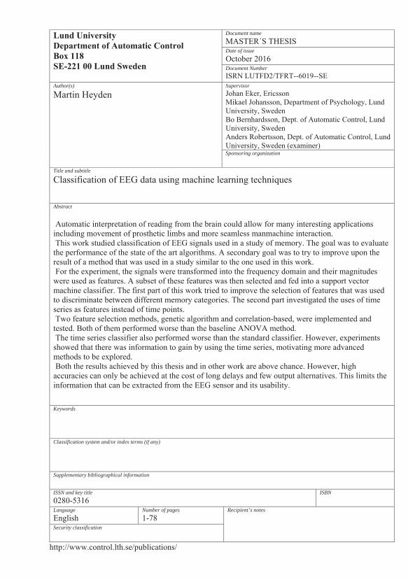
Document name
Date of issue
Document Number
Author(s) Supervisor
Sponsoring organization
Title and subtitle
Abstract
Keywords
Classification system and/or index terms (if any)
Supplementary bibliographical information
ISSN and key title ISBN
Language Number of pages Recipient’s notes
Security classification


![Data Augmentation for EEG-Based Emotion …futuremedia.szu.edu.cn/assets/files/Data Augmentation for...Machine as a classifier to build EEG-based emotion recognition systems [22].](https://static.documents.pub/doc/80x56/5ed36f9c0339371bce117787/data-augmentation-for-eeg-based-emotion-augmentation-for-machine-as-a-classiier.jpg)


