Classification - Simon Fraser University

CLASSIFICATION

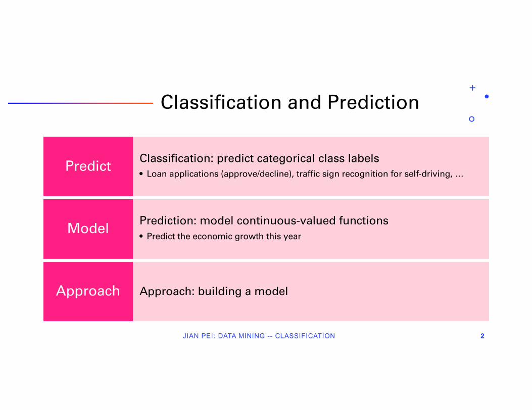
Classification and Prediction

JIAN PEI: DATA MINING -- CLASSIFICATION 2

Classification: predict categorical class labels • Loan applications (approve/decline), traffic sign recognition for self-driving, …

Predict

Prediction: model continuous-valued functions• Predict the economic growth this year

Model

Approach: building a modelApproach

Classification: A 2-step Process


Learning step/model construction: describe a set of

predetermined classes

• Training dataset: tuples for model construction• Each tuple/sample belongs

to a predefined class• Classification rules, decision

trees, or math formulae

Classification step/model application: classify unseen

objects

• Estimate accuracy of the model using an independent test set

• Acceptable accuracy àapply the model to classify tuples with unknown class labels

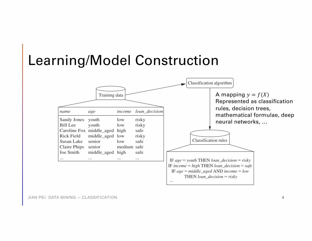
Learning/Model Construction


name loan_decisionage income

Training data

Classification algorithm

Classification rules

...

IF age � youth THEN loan_decision � riskyIF income � high THEN loan_decision � safe

IF age � middle_aged AND income � low THEN loan_decision � risky

Sandy JonesBill LeeCaroline FoxRick FieldSusan LakeClaire PhipsJoe Smith...

youthyouthmiddle_agedmiddle_agedseniorseniormiddle_aged...

lowlowhighlowlowmediumhigh...

riskyriskysaferiskysafesafesafe...

A mapping 𝑦𝑦 = 𝑓𝑓(𝑋𝑋)Represented as classification rules, decision trees, mathematical formulae, deep neural networks, …

Classification/Model Application


Classification rules

(John Henry, middle_aged, low)Loan decision?

risky

Test data New data

Juan BelloSylvia CrestAnne Yee...

seniormiddle_agedmiddle_aged...

lowlowhigh...

name age income loan_decision

saferiskysafe...

Supervised/Unsupervised Learning

JIAN PEI: DATA MINING -- CLASSIFICATION

• Supervised learning (classification)• Supervision: objects in the training data set have labels• New data is classified based on the training set

• Unsupervised learning (clustering)• The class labels of training data are unknown• Given a set of measurements, observations, etc. with the aim of

establishing the existence of classes or clusters in the data

6

Weakly Supervised Learning


• Weaker supervision information for model training

• Semi-supervised classification: building a classifier based on a limited number of labeled training tuples and a large amount of unlabeled training tuples

• Zero-shot learning: during the training phase, there is no labeled training tuples for some class labels

7

Data Preparation

• Data cleaning• Preprocess data in order

to reduce noise and handle missing values

• Relevance analysis (feature selection)

• Remove the irrelevant or redundant attributes

• Data transformation• Generalize and/or

normalize data


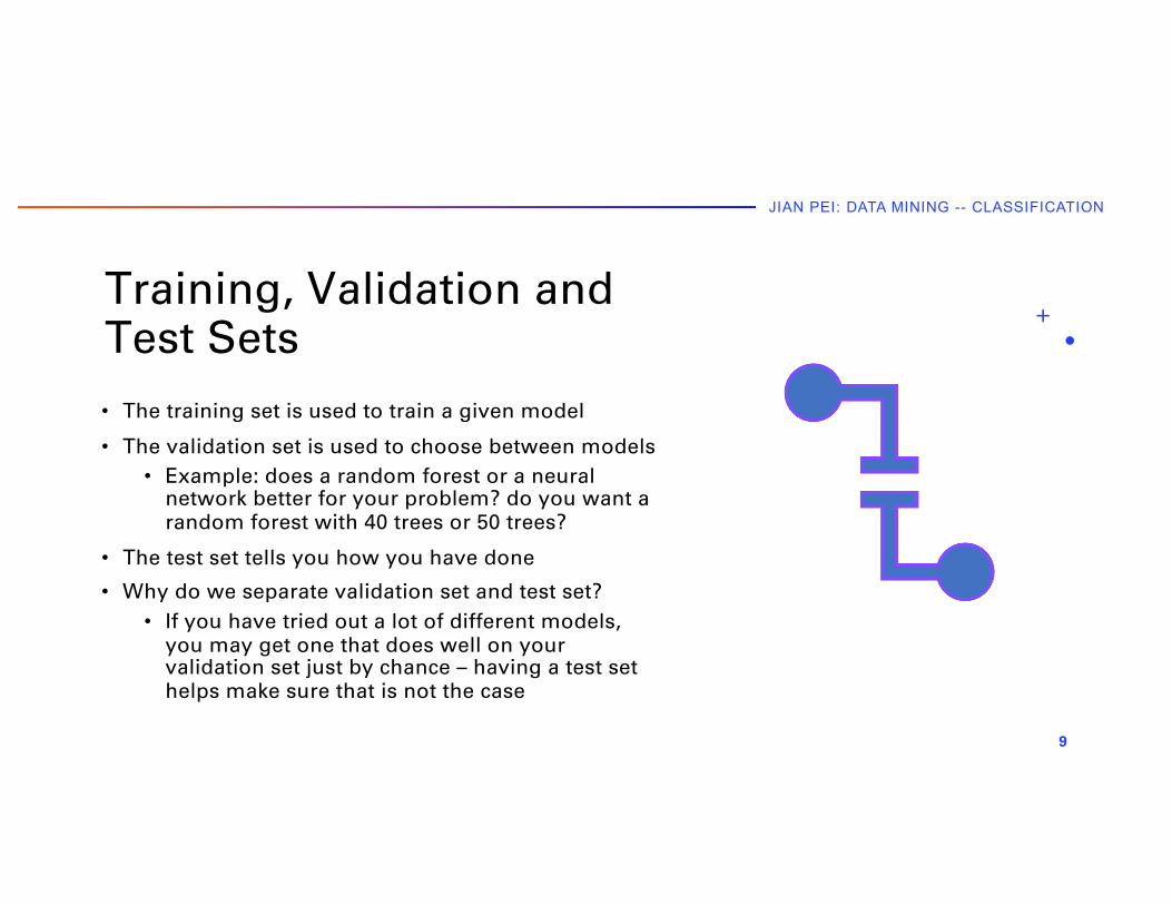
Training, Validation and Test Sets


• The training set is used to train a given model

• The validation set is used to choose between models• Example: does a random forest or a neural

network better for your problem? do you want a random forest with 40 trees or 50 trees?

• The test set tells you how you have done

• Why do we separate validation set and test set?• If you have tried out a lot of different models,

you may get one that does well on your validation set just by chance – having a test set helps make sure that is not the case

9

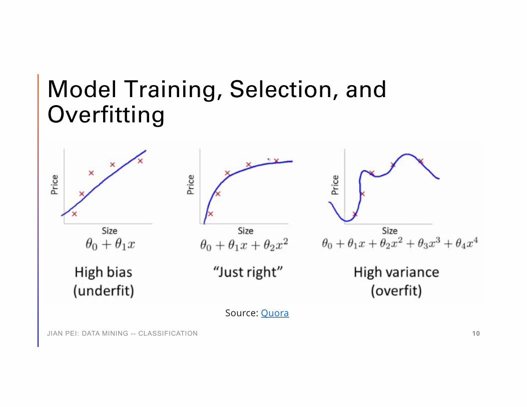
Model Training, Selection, and Overfitting


Source: Quora

Measurements of Quality

• Prediction accuracy• Speed and scalability

• Construction speed and application speed

• Robustness: handle noise and missing values

• Scalability: build model for large training data sets

• Interpretability: understandability of models

JIA

N P

EI:

DA

TA

MIN

ING

--

CLA

SS

IFIC

AT

ION

11

Precision • Target class (also known as positive class)

• Precision: the percentage of the predictions on the target class that is correct

• Example• Target class: risky loan applications• Among 1000 loan applications, the

model classifies 100 as risky, and 85 are truly risky and 15 indeed are not risky, determined by ground truth, then precision is 85 / 100 = 85%

• Precision does not measure those risky cases that are not captured by the model


Decision Tree Induction• Decision tree

representation

• Construction of a decision tree

• Inductive bias and overfitting

• Scalable enhancements for large databases

JIA

N P

EI:

DA

TA

MIN

ING

--

CLA

SS

IFIC

AT

ION

13

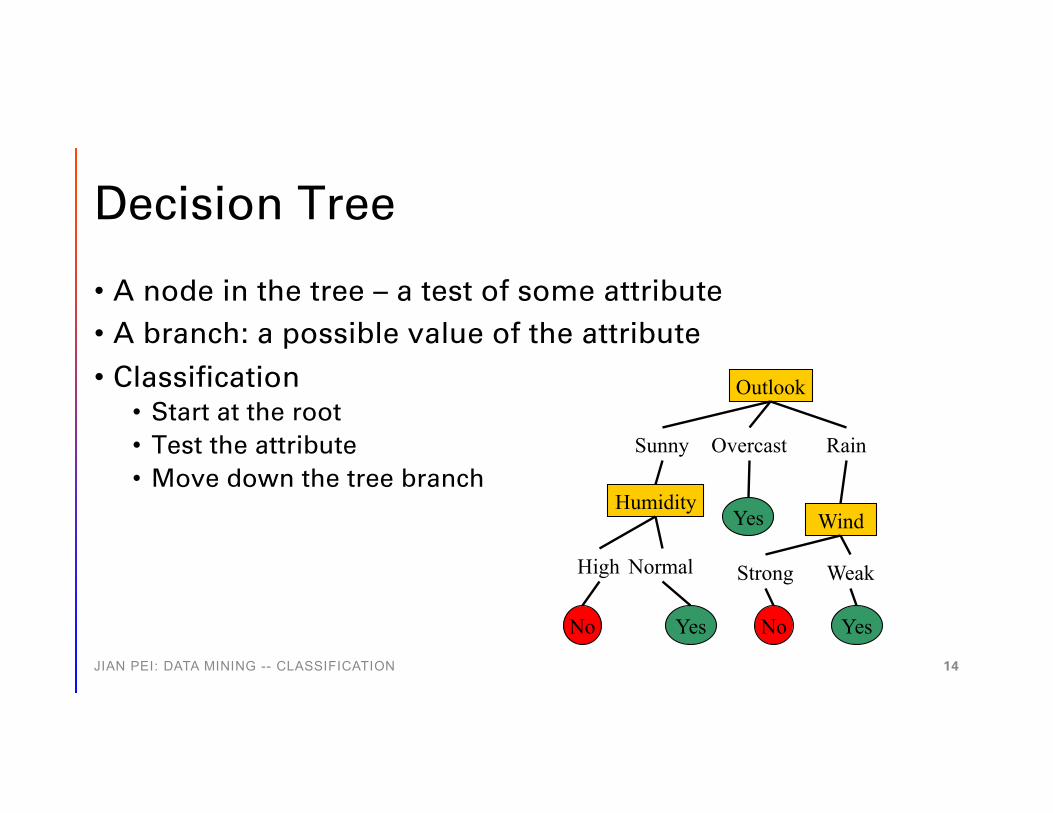
Decision Tree

• A node in the tree – a test of some attribute• A branch: a possible value of the attribute• Classification

• Start at the root• Test the attribute• Move down the tree branch

Outlook

Sunny Overcast Rain

Humidity

High Normal

No Yes

Yes Wind

Strong Weak

No Yes


TRAINING DATASET


Outlook Temp Humid Wind PlayTennisSunny Hot High Weak NoSunny Hot High Strong NoOvercast Hot High Weak YesRain Mild High Weak YesRain Cool Normal Weak YesRain Cool Normal Strong No

Overcast Cool Normal Strong YesSunny Mild High Weak NoSunny Cool Normal Weak YesRain Mild Normal Weak YesSunny Mild Normal Strong YesOvercast Mild High Strong YesOvercast Hot Normal Weak YesRain Mild High Strong No

Appropriate Problems

• Instances are represented by attribute-value pairs

• Extensions of decision trees can handle real-valued attributes

• Disjunctive descriptions may be required

• The training data may contain errors or missing values

JIA

N P

EI:

DA

TA

MIN

ING

--

CLA

SS

IFIC

AT

ION

16

Basic Algorithm ID3• Construct a tree in a top-down recursive

divide-and-conquer manner• Which attribute is the best at the current

node?• Create a node for each possible attribute

value• Partition training data into descendant

nodes

• Conditions for stopping recursion• All samples at a given node belong to

the same class• No attribute remained for further

partitioning• Majority voting is employed for

classifying the leaf• There is no sample at the node

JIA

N P

EI:

DA

TA

MIN

ING

--

CLA

SS

IFIC

AT

ION

17

Partitioning A Node


A discrete-valued attribute

A continuous-valued attribute

A discrete-valued attribute in a binary tree

Which Attribute

Is the Best?

• The attribute most useful for classifying examples

• Information gain and Gini impurity

• Statistical properties• Measure how well an

attribute separates the training examples

JIA

N P

EI:

DA

TA

MIN

ING

--

CLA

SS

IFIC

AT

ION

19

Entropy

• Measure homogeneity of examples

• S is the training data set, and pi is the proportion of S belong to class i

• The smaller the entropy, the purer the data set

å=

-ºc

iii ppSEntropy

12log)(


Information Gain

• The expected reduction in entropy caused by partitioning the examples according to an attribute

åÎ

-º)(

)(||||)(),(

AValuesvv

v SEntropySSSEntropyASGain

Value(A) is the set of all possible values for attribute A, and Sv is the subset of S for which attribute A has value v


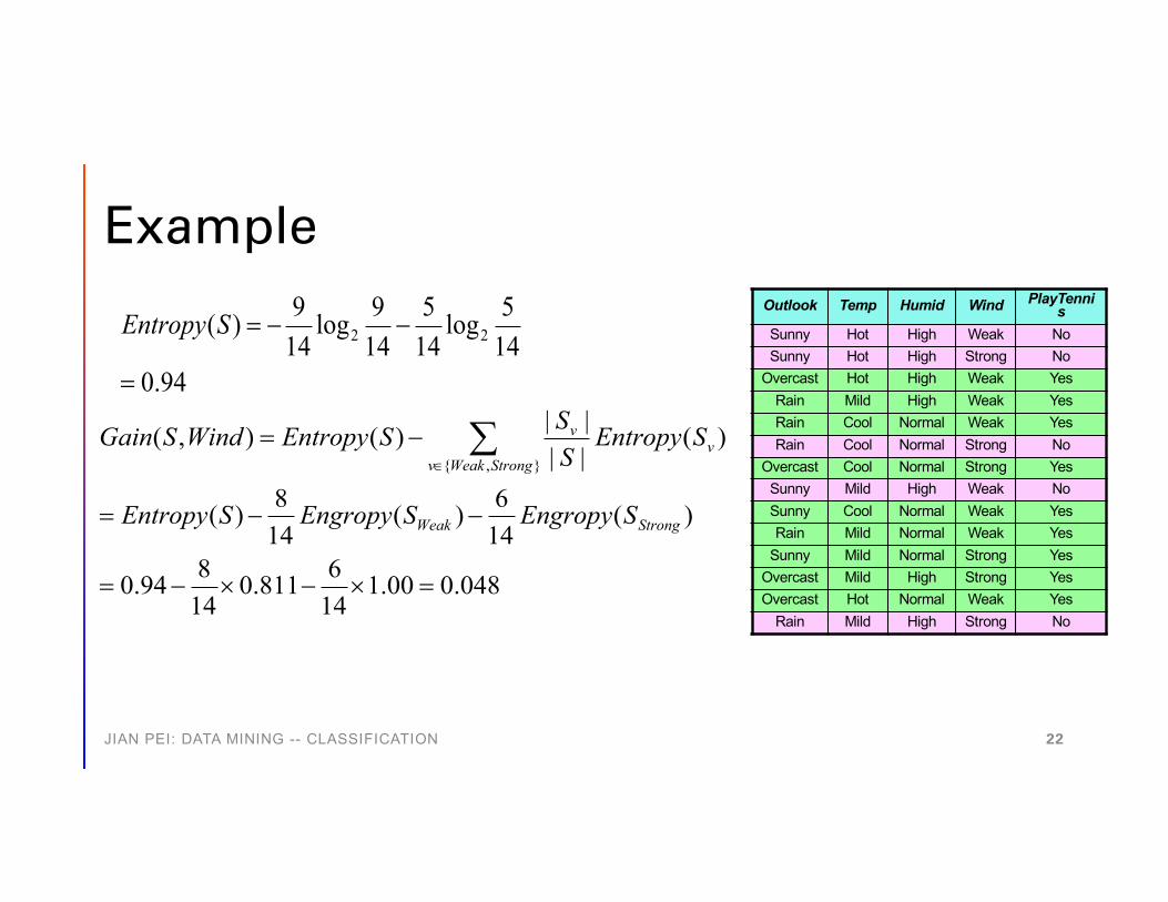
ExampleOutlook Temp Humid Wind PlayTenni

sSunny Hot High Weak NoSunny Hot High Strong No

Overcast Hot High Weak YesRain Mild High Weak YesRain Cool Normal Weak YesRain Cool Normal Strong No

Overcast Cool Normal Strong YesSunny Mild High Weak NoSunny Cool Normal Weak YesRain Mild Normal Weak Yes

Sunny Mild Normal Strong YesOvercast Mild High Strong YesOvercast Hot Normal Weak Yes

Rain Mild High Strong No

94.0145log

145

149log

149)( 22

=

--=SEntropy

048.000.1146811.0

14894.0

)(146)(

148)(

)(||||)(),(

},{

=´-´-=

--=

-= åÎ

StrongWeak

StrongWeakvv

v

SEngropySEngropySEntropy

SEntropySSSEntropyWindSGain


Hypothesis Space Search in Decision Tree Building

• Hypothesis space: the set of possible decision trees

• ID3: simple-to-complex, hill-climbing search

• Evaluation function: information gain

JIA

N P

EI:

DA

TA

MIN

ING

--

CLA

SS

IFIC

AT

ION

23

Capabilities and Limitations

• The hypothesis space is complete

• Maintains only a single current hypothesis

• No backtracking• May converge to a locally

optimal solution

• Use all training examples at each step

• Make statistics-based decisions

• Not sensitive to errors in individual example


Natural Bias

• The information gain measure favors attributes with many values

• An extreme example• Attribute “date” may have the

highest information gain• A very broad decision tree of

depth one• Inapplicable to any future data


Alternative Measures

• Gain ratio: penalize attributes like date by incorporating split information

• Split information is sensitive to how broadly and uniformly the attribute splits the data

• Gain ratio can be undefined or very large• Only test attributes with over average gain

||||log

||||),(

12 SS

SSASmationSplitInfor i

c

i

iå=

-º

),(),(),(

ASmationSplitInforASGainASGainRatio º


Measuring InequalityLorenz CurveX-axis: quintilesY-axis: accumulative share of income earned by the plotted quintileGap between the actual lines and the mythical line: the degree of inequality

Giniindex

Gini = 0, even distributionGini = 1, perfectly unequalThe greater the distance, the more unequal the distribution


Gini Impurity

• A data set S contains examples from n classes

• pj is the relative frequency of class j in S

• A data set S is split into two subsets S1 and S2 with sizes N1and N2 respectively

• The attribute provides the smallest ginisplit(T) is chosen to split the node

å=

-=n

jp jTgini121)(

)()()( 22

11 Tgini

NNTgini

NNTginisplit +=


Extracting Classification Rules


Classification rules can be extracted from a decision tree

• All attribute-value pairs along a path form a conjunctive condition• The leaf node holds the class prediction• IF age = “<=30” AND student = “no” THEN buys_computer = “no”

Each path from the root to a leaf à an IF-THEN rule

Rules are easy to understand

C4.5: Successor to ID3JIAN PEI: DATA MINING -- CLASSIFICATION

• Capability of handling continuous numerical attributes• For a continuous numerical attribute, define a discrete attribute that

partitions the continuous attribute value into a discrete set of intervals• Convert the trained tree into sets of if-then rules

• The accuracy of each rule is evaluated to determine the order of rules in which they should be applied

• Pruning a rule’s precondition if the accuracy of the rule improves without the precondition

• Source code in C available at “C4.5: Programs for Machine Learning”• J48 is the open source Java implementation in Weka

30

C5.0/See5: Commercial Products

• Significantly faster and memory more efficient than C4.5

• Smaller decision trees

• Support for boosting

• Support for weighting cases and misclassification types

• Winnowing: automatically removing unhelpful attributes

JIA

N P

EI:

DA

TA

MIN

ING

--

CLA

SS

IFIC

AT

ION

31

Regression Tree


• Predict continuous output value

• Very similar to a decision tree

• A leaf node holds a continuous value set as the average output value of all training tuples fallen in the corresponding sub-regions

32

REGRESSION TREE

EXAMPLE


CART: Classification and Regression Trees

• Very similar to C4.5• Binary trees only• Supporting numerical

target variables through regression

• No rule sets• Using residual sum of

squares (RSS)


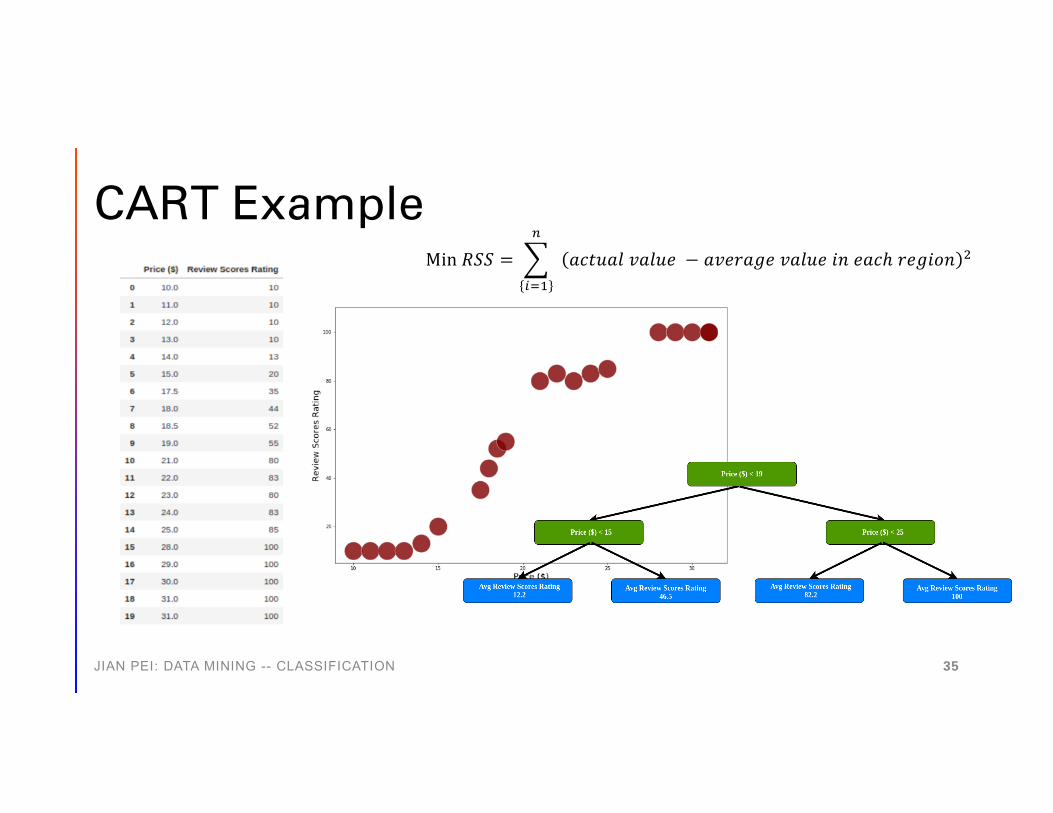
CART Example


Min 𝑅𝑅𝑅𝑅𝑅𝑅 = ,!"#

$

𝑎𝑎𝑎𝑎𝑎𝑎𝑎𝑎𝑎𝑎𝑎𝑎 𝑣𝑣𝑎𝑎𝑎𝑎𝑎𝑎𝑣𝑣 − 𝑎𝑎𝑣𝑣𝑣𝑣𝑎𝑎𝑎𝑎𝑎𝑎𝑣𝑣 𝑣𝑣𝑎𝑎𝑎𝑎𝑎𝑎𝑣𝑣 𝑖𝑖𝑖𝑖 𝑣𝑣𝑎𝑎𝑎𝑎𝑒 𝑎𝑎𝑣𝑣𝑎𝑎𝑖𝑖𝑟𝑟𝑖𝑖 %

Inductive Bias

• The set of assumptions that, together with the training data, deductively justifies the classification to future instances

• Preferences of the classifier construction

• Shorter trees are preferred over longer trees

• Trees that place high information gain attributes close to the root are preferred

JIA

N P

EI:

DA

TA

MIN

ING

--

CLA

SS

IFIC

AT

ION

36

Why Prefer Short Trees?

• Occam’s razor: prefer the simplest hypothesis that fits the data

• Fewer short trees than long trees• A short tree is less likely to be a statistical coincidence

“One should not increase, beyond what is necessary, the number of entities required to explain anything”– Also known as the principle of parsimony


Overfitting • A decision tree T may overfit the training data

• if there exists an alternative tree T’ such that T has a higher accuracy than T’ over the training examples, but T’has a higher accuracy than T over the entire distribution of data

• Why overfitting?• Noise data• Bias in training data


All data Training data

TT’

Avoid Overfitting • Prepruning: stop growing the tree

earlier• Difficult to choose an appropriate

threshold

• Postpruning: remove branches from a “fully grown” tree

• Use an independent set of data to prune

• Key: how to determine the correct final tree size


Determine the Final Tree Size

• Separate training (2/3) and testing (1/3) sets

• Use cross validation, e.g., 10-fold cross validation

• Use all the data for training• Apply a statistical test (e.g.,

chi-square) to estimate whether expanding or pruning a node may improve the entire distribution

• Use minimum description length (MDL) principle

• halting growth of the tree when the encoding is minimized

JIA

N P

EI:

DA

TA

MIN

ING

--

CLA

SS

IFIC

AT

ION

40

Enhancements

• Allow for attributes of continuous values• Dynamically discretize continuous attributes

• Handle missing attribute values• Attribute construction

• Create new attributes based on existing ones that are sparsely represented

• Reduce fragmentation, repetition, and replication


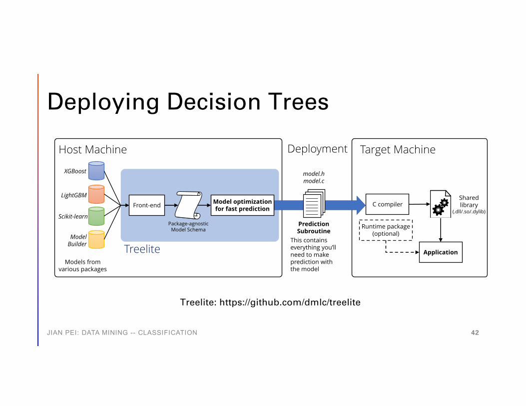
Deploying Decision Trees


Prediction Subroutine

model.hmodel.c

This contains everything you’ll need to make prediction with the model

Deployment

Front-end

Host Machine

XGBoost

LightGBM

Scikit-learn

ModelBuilder

Package-agnosticModel Schema

Models fromvarious packages

Treelite

Target Machine

Shared library

(.dll/.so/.dylib)

Application

Runtime package(optional)

Model optimization for fast prediction

C compiler

Treelite: https://github.com/dmlc/treelite

Accuracy May Be Misleading …

• Accuracy: the percentage that a classifier predicts the classes correctly

• Consider a data set of 99% of the negative class and 1% of the positive class

• A classifier predicts everything negative has an accuracy of 99%, though it does not work for the positive class at all!

• Imbalance class distribution is popular in many applications• Medical applications, fraud detection, …


Performance Evaluation Matrix

PREDICTED CLASS Total

ACTUALCLASS

Class=Positive Class=NegativeClass=Positive TP FN PClass=Negative FP TN N

Total P’ N’ P+N

Confusion matrix (contingency table, error matrix): used for imbalance class distribution


𝐴𝐴𝐴𝐴𝐴𝐴𝐴𝐴𝐴𝐴𝐴𝐴𝐴𝐴𝐴𝐴 =𝑇𝑇𝑇𝑇 + 𝑇𝑇𝑇𝑇𝑇𝑇 + 𝑇𝑇

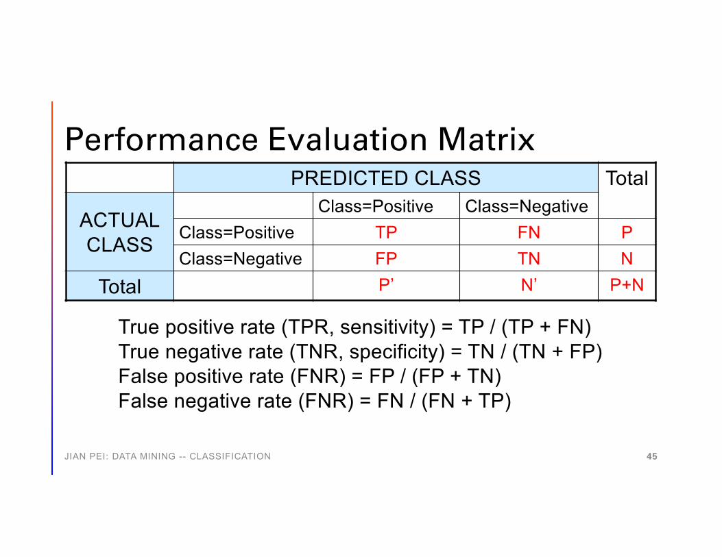
Performance Evaluation Matrix

True positive rate (TPR, sensitivity) = TP / (TP + FN)True negative rate (TNR, specificity) = TN / (TN + FP)False positive rate (FNR) = FP / (FP + TN)False negative rate (FNR) = FN / (FN + TP)



ACTUALCLASS


Total P’ N’ P+N

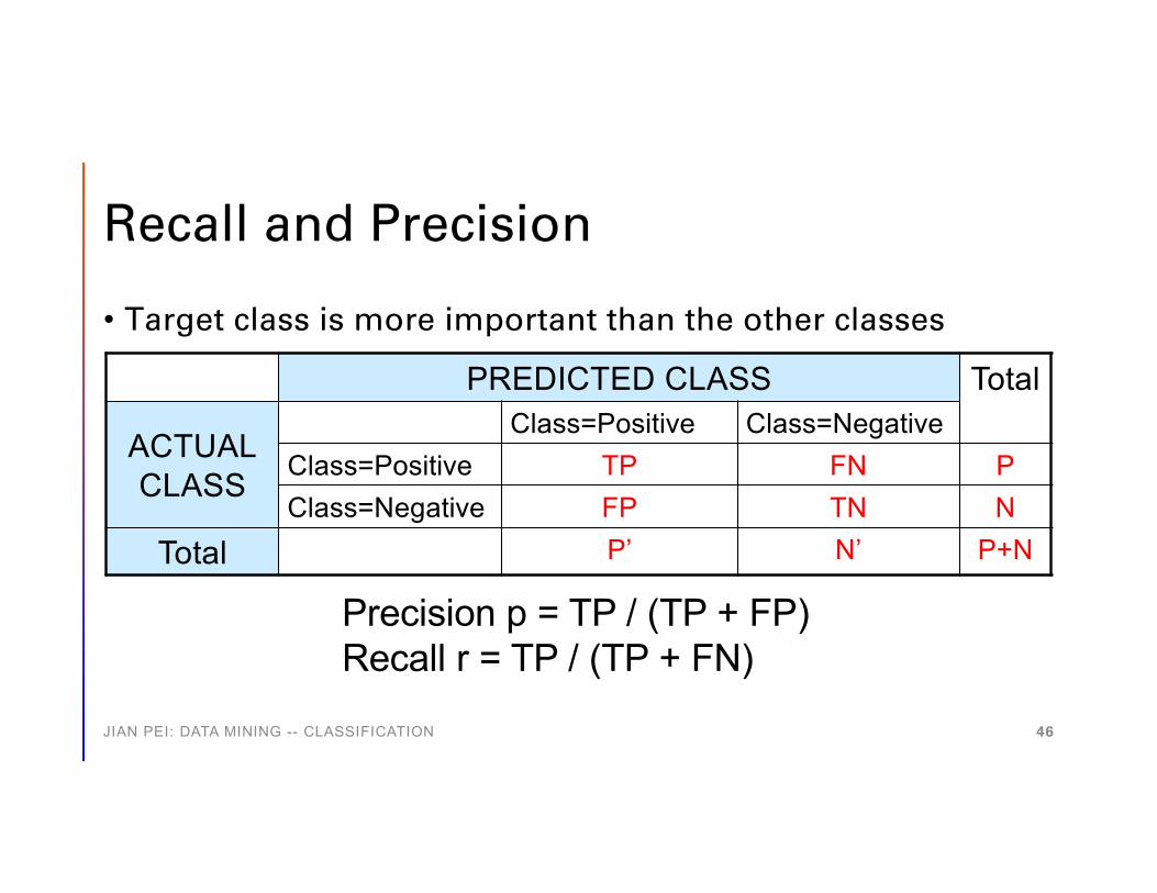
Recall and Precision

• Target class is more important than the other classes

Precision p = TP / (TP + FP)Recall r = TP / (TP + FN)



ACTUALCLASS


Total P’ N’ P+N

Type I and Type II ErrorsJIAN PEI: DATA MINING -- CLASSIFICATION

• Type I errors – false positive: a negative object is classified as positive• Fallout: the type I error rate, FP / (TP + FP)

• Type II errors – false negative: a positive object is classified as negative• Captured by recall

• A classifier may trade off between Type I and Type II errors

• Crossover error rate (CER): the point at which Type I errors and Type II errors are equal • The best way of measuring a biometrics' effectiveness• A system with a lower CER value provides more accuracy than a system with a higher

CER value

47

Fβ Measure

• How can we summarize precision and recall into one metric?

• Using the harmonic mean between the two

• Fβ measure

• β = 0, Fβ is the precision• β = ∞, Fβ is the recall• 0 < β < ∞, Fβ is a tradeoff between the precision and the recall

FNFPTPTP

prrp

++=

+=

222(F) measure-F

Fβ =(β 2 +1)rpr +β 2p

=(β 2 +1)TP

(β 2 +1)TP +β 2FN +FP


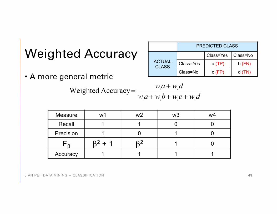
Weighted Accuracy

• A more general metric

dwcwbwawdwaw

4321

41Accuracy Weighted+++

+=

Measure w1 w2 w3 w4Recall 1 1 0 0Precision 1 0 1 0

Fβ β2 + 1 β2 1 0

Accuracy 1 1 1 1


PREDICTED CLASS

ACTUALCLASS

Class=Yes Class=No

Class=Yes a (TP) b (FN)

Class=No c (FP) d (TN)

The Evaluation Issues

• The accuracy of a classifier can be evaluated using a test data set

• The test set is a part of the available labeled data set

• But how can we evaluate the accuracy of a classification method?

• A classification method can generate many classifiers using different parameters?

• What if the available labeled data set is too small?


Holdout Method

• Partition the available labeled data set into two disjoint subsets: the training set and the test set

• 50-50• 2/3 for training and 1/3 for testing

• Build a classifier using the training set• Evaluate the accuracy using the test set


Limitations of Holdout Method

• Fewer labeled examples for training• The classifier highly depends on the composition of the

training and test sets• The smaller the training set, the larger the variance

• If the test set is too small, the evaluation is not reliable• The training and test sets are not independent


Cross-Validation


• Each record is used the same number of times for training and exactly once for testing

• K-fold cross-validation• Partition the data into k equal-sized subsets• In each round, use one subset as the test set, and use the rest subsets together

as the training set

• Repeat k times• The total error is the sum of the errors in k rounds

• Leave-one-out: k = n• Utilize as much data as possible for training

• Computationally expensive

• Dangers of cross-validation: dependency among training samples

53

Confidence Interval for Accuracy

• Suppose a classifier C is tested on a test set of n cases, and the accuracy is acc

• How much confidence can we have on acc?• We need to estimate the confidence interval of a given model

accuracy• Within the confidence interval, one is sufficiently sure that the true

population value lies or, equivalently, by placing a bound on the probable error of the estimate

• A confidence interval procedure uses the data to determine an interval with the property that – viewed before the sample is selected – the interval has a given high probability of containing the true population value


Binomial Experiments

• When a coin is flipped, it has a probability p to have the head turned up

• If the coin is flipped N times, what is the probability that we see the head X times?

• Expectation (mean): Np• Variance: Np(1 - p)

vNv ppvN

vXP --÷÷ø

öççè

æ== )1()(


Confidence Level and ApproximationArea = 1 - aa

Zaa/2 Z1- aa /2

a

aa

-=

<--

<-

1

)/)1(

(2/12/

ZNpp

paccZP

)(2442

22/

222/2/

22/

a

aaa

ZNaccNaccNZZZaccN

+×-×+±+×

Zα: the bound at confidence level (1-α)

Approximating using normal distribution


ROC Curve

• Receiver Operating Characteristic (ROC)1-dimensional data set containing 2 classes. Any points located at x > t is classified as positive


True positive rate (TPR, sensitivity) = TP / (TP + FN)False positive rate (FNR) = FP / (FP + TN)

ROC Curve(TP,FP):• (0,0): declare everything

to be negative class• (1,1): declare everything

to be positive class• (1,0): ideal• Diagonal line:

• Random guessing• Below diagonal line: prediction is

opposite of the true class


True positive rate (TPR, sensitivity) = TP / (TP + FN)False positive rate (FNR) = FP / (FP + TN)

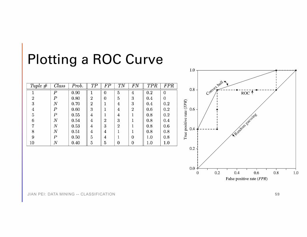
Plotting a ROC Curve


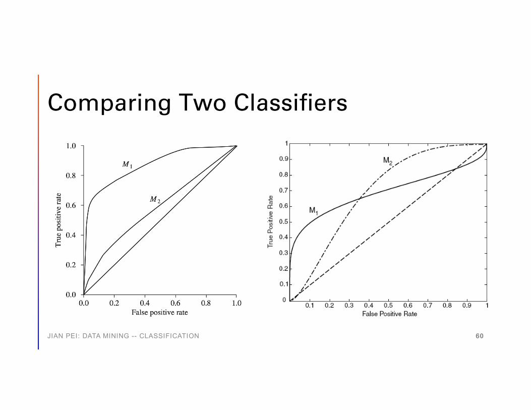
Comparing Two Classifiers


Significance Tests

• Are two algorithms different in effectiveness?• The null hypothesis: there is NO difference• The alternative hypothesis: there is a difference – B is better than A (the baseline

method)

• Matched pair experiments: the rankings that are compared are based on the same set of queries for both algorithms

• Possible errors of significant tests• Type I: the null hypothesis is rejected when it is true• Type II: the null hypothesis is accepted when it is false

• The power of a hypothesis test: the probability that the test will reject the null hypothesis correctly• Reducing the type II errors


Procedure of Comparison

• Using a set of data sets• Procedure

• Compute the effectiveness measure for every data set• Compute a test statistic based on a comparison of the effectiveness measures

for each data set• E.g., the t-test, the Wilcoxon signed-rank test, and the sign test

• Compute a P-value: the probability that a test statistic value at least that extreme could be observed if the null hypothesis were true

• The null hypothesis is rejected if the P-value £ a, where a is the significance level which is used to minimize the type I errors

• One-sided (one-tailed) tests: whether B is better than A (the baseline method)• Two-sided tests: whether A and B are different – the P-value is doubled


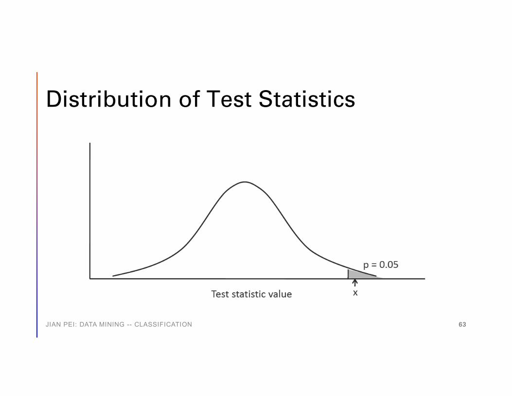
Distribution of Test Statistics


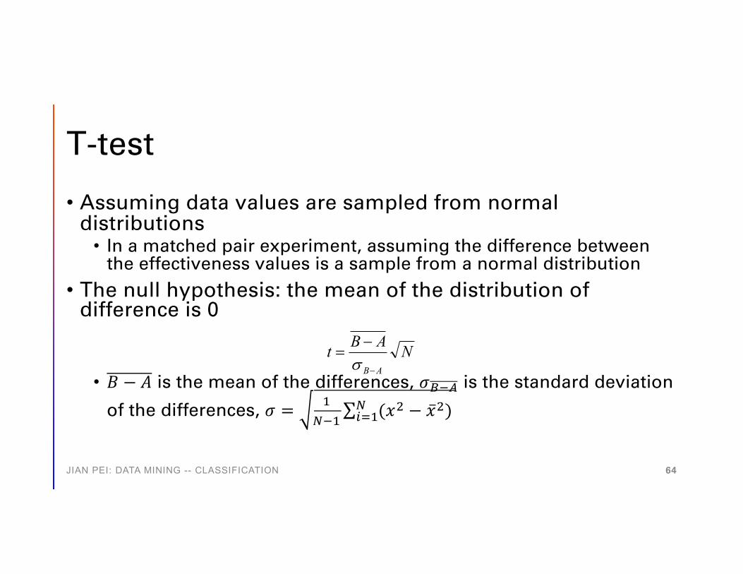
T-test

• Assuming data values are sampled from normal distributions

• In a matched pair experiment, assuming the difference between the effectiveness values is a sample from a normal distribution

• The null hypothesis: the mean of the distribution of difference is 0

• 𝐵𝐵 − 𝐴𝐴 is the mean of the differences, 𝜎𝜎;<= is the standard deviation

of the differences, 𝜎𝜎 = >?<>

∑@A>? (𝑥𝑥B − �̅�𝑥B)

NABtAB-

-=s


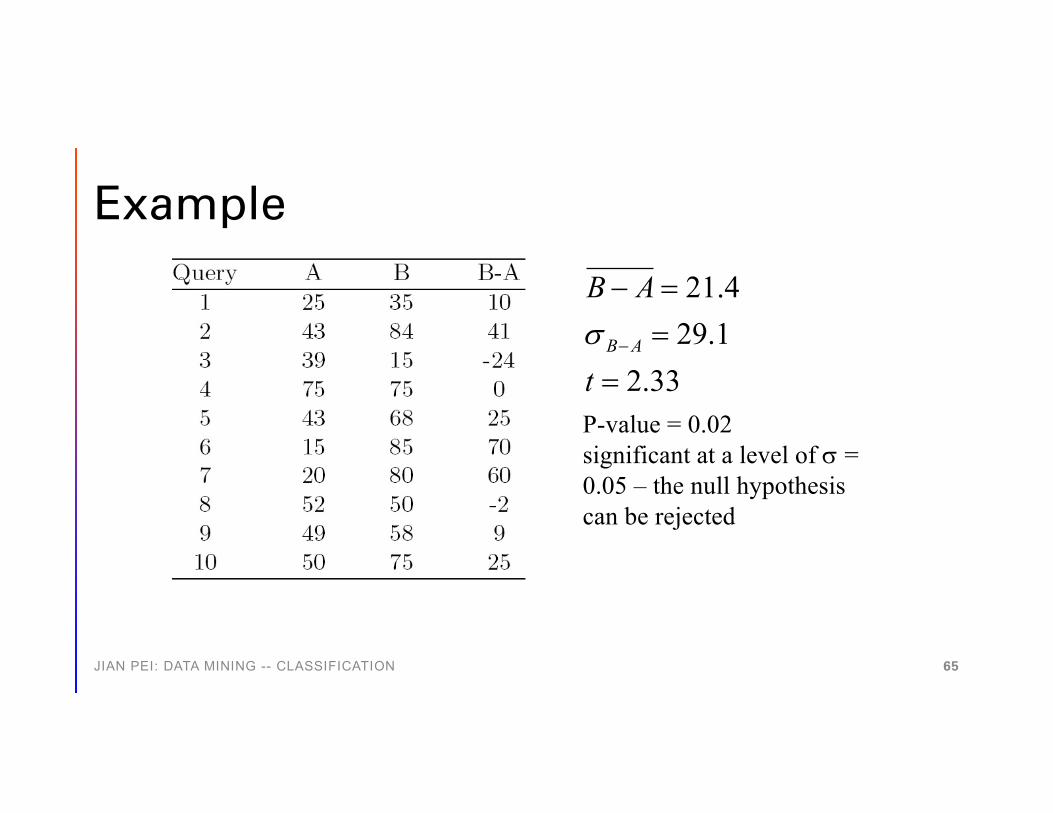
Example

33.21.294.21

===-

-

t

AB

ABs

P-value = 0.02 significant at a level of s = 0.05 – the null hypothesis can be rejected


Issues in T-test

• Data is assumed to be sampled from normal distributions• Generally inappropriate for effectiveness measures• However, experiments showed that t-test produces very similar

results to the randomization test which does not assume any distribution (the most powerful nonparametric test)

• T-test assumes that the evaluation data is measured on an interval scale

• Effectiveness measures are ordinal – the magnitude of the differences are not significant

• Use the Wilcoxon signed-rank test and the sign test, which make less assumption about the effectiveness measure, but are less powerful


Wilcoxon Signed-Rank Test

• Assumption: the differences between the effectiveness values can be ranked, but the magnitude is not important

• Ri is a signed-rank, N is the number of non-zero differences

• Procedure• The differences are sorted by their absolute values increasing order• Differences are assigned rank values (ties are assigned the average rank)• The rank values are given the sign of the original difference

• The null hypothesis: the sum of the positive ranks will be the same as the sum of the negative ranks

å=

=N

iiRw

1


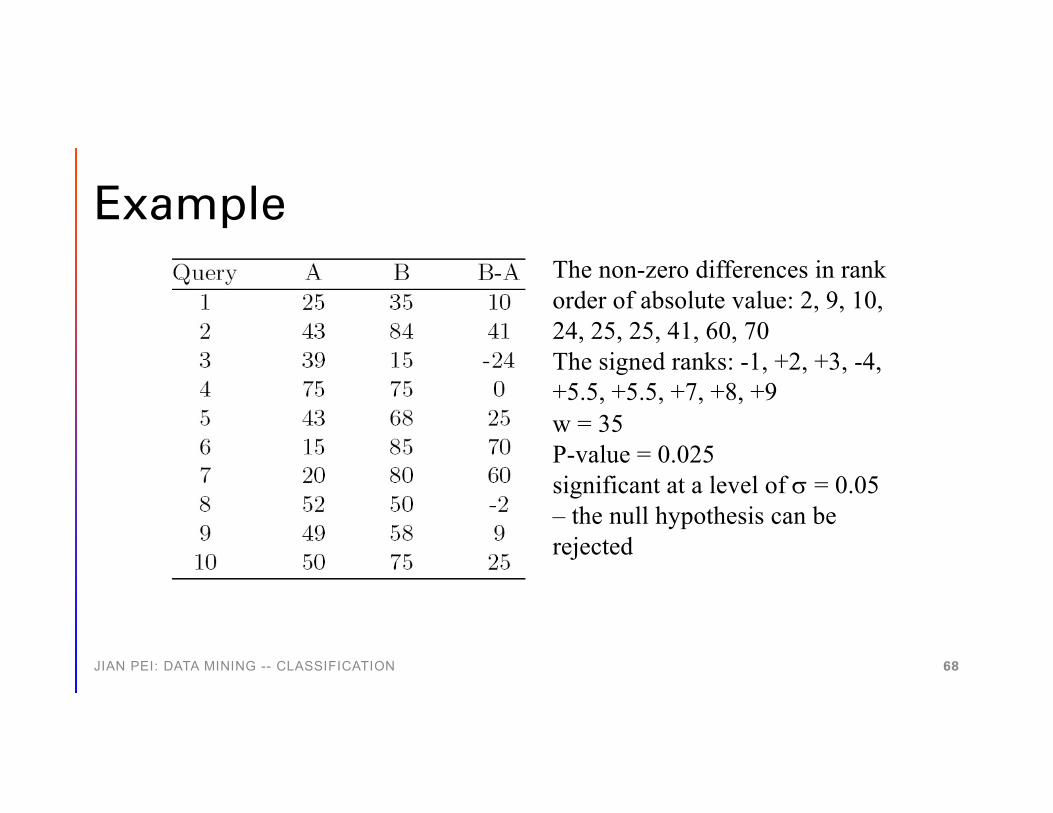
ExampleThe non-zero differences in rank order of absolute value: 2, 9, 10, 24, 25, 25, 41, 60, 70The signed ranks: -1, +2, +3, -4, +5.5, +5.5, +7, +8, +9w = 35P-value = 0.025significant at a level of s = 0.05 – the null hypothesis can be rejected


Sign Test

• Completely ignore the magnitude of the differences• In practice, we may require that a 5-10% difference is needed to be

considered as different

• The null hypothesis: P(B > A) = P(A > B) = ½• Sum up the number of pairs B > A


Example7 pairs out of 10 B > AP-value = 0.17 – the probability that we observe 7 successes out of 10 trials where the probability of success is 0.5Cannot reject the null hypothesis


Cost-Sensitive Learning

• In some applications, misclassifying some classes may be disastrous

• Tumor detection, fraud detection

• Using a cost matrix

PREDICTED CLASS

ACTUALCLASS

Class=Yes Class=NoClass=Yes -1 100Class=No 1 0


Sampling for Imbalance Classes

• Consider a data set containing 100 positive examples and 1,000 negative examples

• Undersampling: use a random sample of 100 negative examples and all positive examples

• Some useful negative examples may be lost• Run undersampling multiple times, use the ensemble of multiple

base classifiers• Focused undersampling: remove negative samples that are not

useful for classification, e.g., those far away from the decision boundary


Oversampling

• Replicate the positive examples until the training set has an equal number of positive and negative examples

• For noisy data, may cause overfitting


Errors in Classification

• Bias: the difference between the real class boundary and the decision boundary of a classification model

• Variance: variability in the training data set• Intrinsic noise in the target class: the target class can be

non-deterministic – instances with the same attribute values can have different class labels


Bias

Figure from [Tan, Steinbach, Kumar]JIAN PEI: DATA MINING -- CLASSIFICATION 75

One or More?

• What if a medical doctor is not sure about a case?• Joint-diagnosis: using a group of doctors carrying different

expertise• Wisdom from crowd is often more accurate

• All eager learning methods make prediction using a single classifier induced from training data

• A single classifier may have low confidence in some cases

• Ensemble methods: construct a set of base classifiers and take a vote on predictions in classification


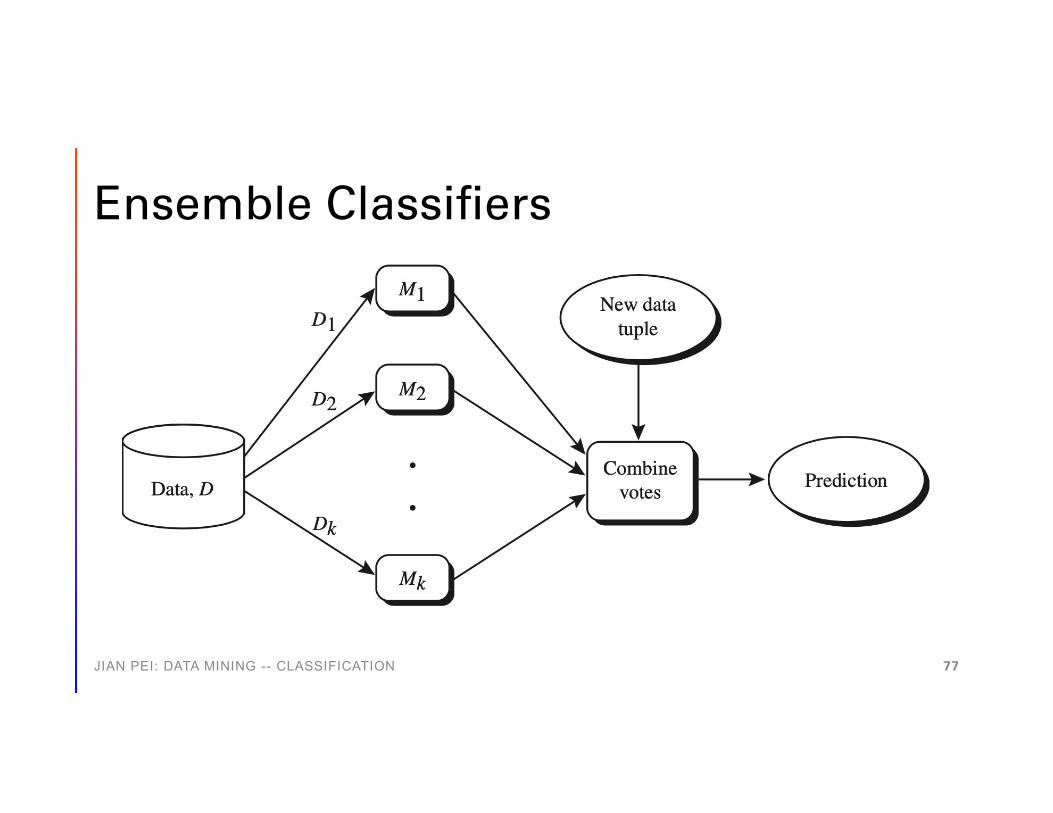
Ensemble Classifiers


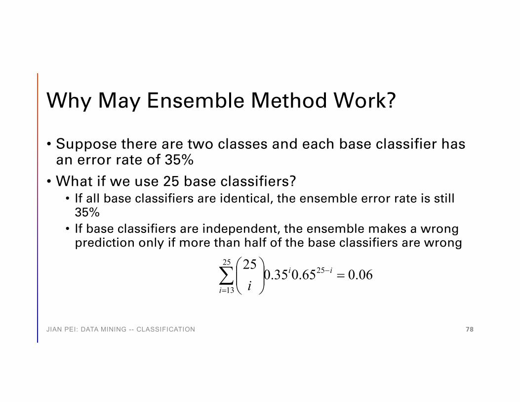
Why May Ensemble Method Work?

• Suppose there are two classes and each base classifier has an error rate of 35%

• What if we use 25 base classifiers?• If all base classifiers are identical, the ensemble error rate is still

35%• If base classifiers are independent, the ensemble makes a wrong

prediction only if more than half of the base classifiers are wrong

å=

- =÷÷ø

öççè

æ25

13

25 06.065.035.025

i

ii

i


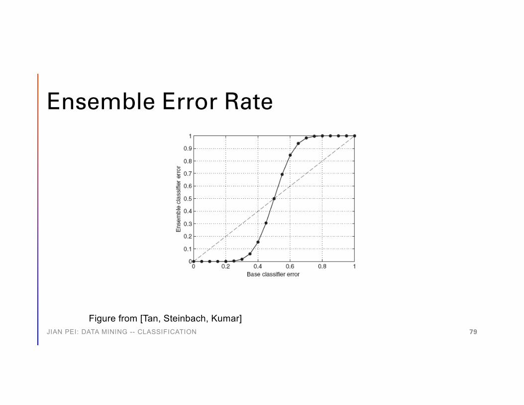
Ensemble Error Rate


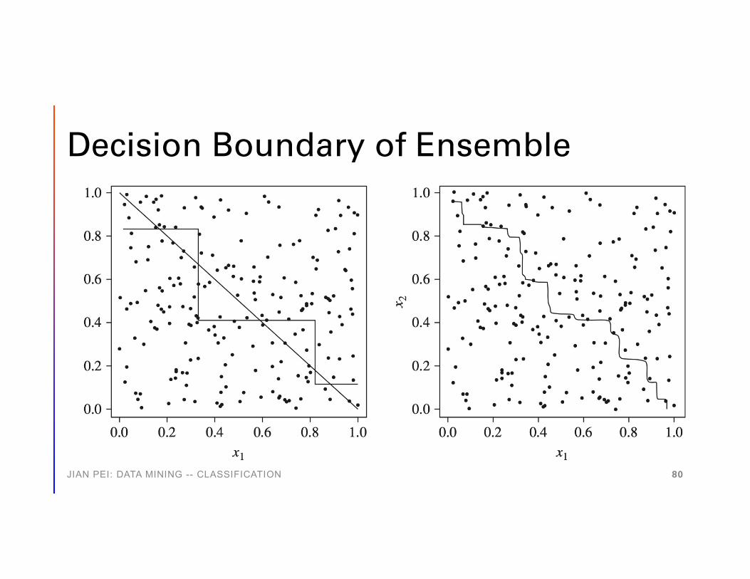
Decision Boundary of Ensemble


Ensemble Classifiers – When?

• The base classifiers should be independent of each other• Each base classifier should do better than a classifier that

performs random guessing


How to Construct Ensemble?

• Manipulating the training set: derive multiple training sets and build a base classifier on each

• Manipulating the input features: use only a subset of features in a base classifier

• Manipulating the class labels: if there are many classes, in a classifier, randomly divide the classes into two subsets A and B; for a test case, if a base classifier predicts its class as A, all classes in A receive a vote

• Manipulating the learning algorithm, e.g., using different network configuration in ANN


Bootstrap

• Given an original training set T, derive a training set T’ by repeatedly uniformly sampling with replacement

• If T has n tuples, each tuple has a probability of 𝑝𝑝 = 1 −1 − !

"

"being selected in T’

• When n à ∞, p à 1 - 1/e ≈ 0.632

• Use the tuples not in T’ as the test set


Bootstrap

• Use a bootstrap sample as the training set, use the tuples not in the training set as the test set

• .632 bootstrap: compute the overall accuracy by combining the accuracies of each bootstrap sample with the accuracy computed from a classifier using the whole data set as the training set

)368.0632.0(11

632. all

k

ibootstrap acck

acc ´+´= å e


Bagging (Bootstrap Aggregation)

• Run bootstrap k times to obtain k base classifiers• A test instance is assigned to the class that receives the

highest number of votes• Strength: reduce the variance of base classifiers –good for

unstable base classifiers• Unstable classifiers: sensitive to minor perturbations in the

training set, e.g., decision trees, associative classifiers, and ANN

• For stable classifiers (e.g., linear discriminant analysis and kNN classifiers), bagging may even degrade the performance since the training sets are smaller

• Less overfitting on noisy data


Boosting

• Assign a weight to each training example• Initially, each example is assigned a weight 1/n

• Weights can be used in one of the following ways• Weights as a sampling distribution to draw a set of bootstrap

samples from the original training set• Weights used by a base classifier to learn a model biased towards

heavier examples• Adaptively change the weight at the end of each boosting

round• The weight of an example correctly classified decreases• The weight of an example incorrectly classified increases

• Each round generates a base classifier


Critical Design Choices in Boosting

• How the weights of the training examples are updated at the end of each boosting round?

• How the predictions made by base classifiers are combined?


AdaBoost

• Each base classifier carries an importance score related to its error rate

• Error rate

• wi: weight, I(p) = 1 if p is true• Importance score

( )å=

¹=N

jjjiji yxCIw

N 1)(1e

÷÷ø

öççè

æ -=

i

ii e

ea 1ln21


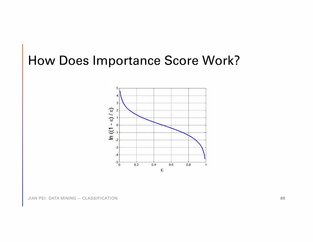
How Does Importance Score Work?


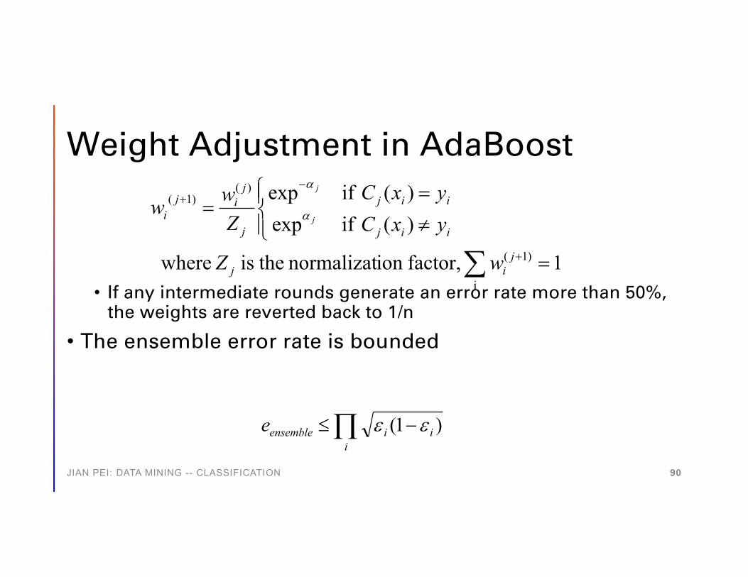
Weight Adjustment in AdaBoost

• If any intermediate rounds generate an error rate more than 50%, the weights are reverted back to 1/n

• The ensemble error rate is bounded

å =

ïî

ïíì

¹=

=

+

-+

i

)1(

)()1(

1 factor,ion normalizat theis where

)( ifexp)( ifexp

jij

iij

iij

j

jij

i

wZ

yxCyxC

Zww

j

j

a

a

Õ -£i

iiensemblee )1( ee


Gradient Boosting

• Start with a simple regression model F(x) and output a constant (i.e., the average output of all training samples)

• Try to find a new base model at each round• Compute the predicted output -𝑦𝑦@ of each training sample by the

current model F(x) and the negative gradient 𝑟𝑟@ = 𝑦𝑦@ − -𝑦𝑦@ of the loss function with respect to the predicted output -𝑦𝑦@

• Fit a regression tree model for the training data set {(𝑥𝑥@ , 𝑟𝑟@)}• The negative gradient 𝑟𝑟@ changes in different rounds, and thus

leads to different base models

• The new base model is added to F(x)


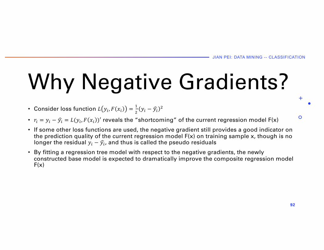
Why Negative Gradients?JIAN PEI: DATA MINING -- CLASSIFICATION

• Consider loss function 𝐿𝐿 𝑦𝑦! , 𝐹𝐹 𝑥𝑥! = #%𝑦𝑦! − G𝑦𝑦! %

• 𝑎𝑎! = 𝑦𝑦! − G𝑦𝑦! = 𝐿𝐿(𝑦𝑦! , 𝐹𝐹 𝑥𝑥! )′ reveals the “shortcoming” of the current regression model F(x)

• If some other loss functions are used, the negative gradient still provides a good indicator on the prediction quality of the current regression model F(x) on training sample x, though is no longer the residual 𝑦𝑦! − G𝑦𝑦!, and thus is called the pseudo residuals

• By fitting a regression tree model with respect to the negative gradients, the newly constructed base model is expected to dramatically improve the composite regression model F(x)

92

XGBoostJIAN PEI: DATA MINING -- CLASSIFICATION

• Learn a weight for each base model, and F(x) is the weighted sum of all base models

• In practice, shrinking the newly constructed base models, 𝐹𝐹 𝑥𝑥 ←𝐹𝐹 𝑥𝑥 + 𝜂𝜂𝑀𝑀I 𝑥𝑥 when a new base model is added (0 < 𝜂𝜂 < 1)

• Control the number of leaf nodes of the regression trees to 4-8

• Use a subsample of the entire training set to construct a new base model in each round

• https://www.amazon.science/publications/treelite-toolbox-for-decision-tree-deployment

93

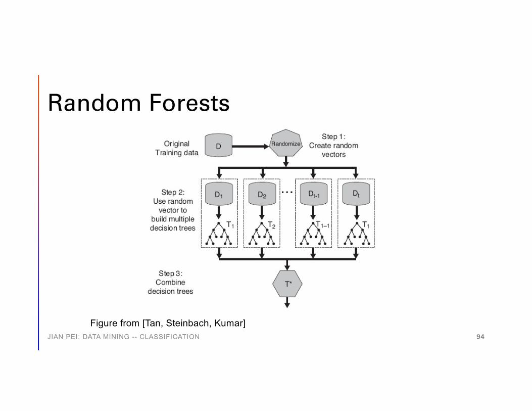
Random Forests


Random Forests

• Using decision trees as base classifiers• Each tree uses only a subset of features in classification• Bagging can be used to generate training sets for decision

trees


Forest-RI (Random Input)

• Each tree is built using a random subset of features• A tree is grown to its entirety without pruning• The smaller the sets of features used by decision trees, the

less correlated the trees• The larger the sets of features used by decision trees, the

more accurate the trees• Tradeoff: m = log2d + 1

• d: number of features in the training set

• If d is too small, it is hard to obtain independent feature sets


Forest-RC

• When the number of features in the training set is too small, use linear combinations of features to generate new features to build decision trees

• Randomly select a set of features L• Linearly combine features in L using coefficients generated

from a uniform distribution in the range of [-1, 1]• At each node, m such randomly combined new features are

generated, and the best of them is used to split the node


Bayesian Classification: Intuition

• More hockey fans in Canada than in US• Which country is Tom, a hockey ball fan, from?• Predicting Canada has a better chance to be right

• Prior probability P(Canadian) = 5%: reflecting background knowledge 5% of total population is Canadians

• P(hockey fan | Canadian) = 30%: the probability of a Canadian being a hockey fan

• Posterior probability P(Canadian | hockey fan): the probability of a hockey fan from Canada


Bayes Theorem

• Find the maximum a posteriori (MAP) hypothesis

• Require background knowledge• Computational cost

)()()|()|(

DPhPhDPDhP =

)()|(max)()()|(max)|(max

hPhDPDP

hPhDPDhPh

Hh

HhHhMAP

Î

ÎÎ

=

=º


Why Bayes Classifier?

• Theoretically, Bayes classifier is optimal in the sense that it has the smallest classification error rate in comparison to all other classifiers

• Bayes classifier plays a fundamental role in statistical machine learning

• In the Bayes’ theorem 𝑇𝑇 𝐻𝐻 𝑋𝑋 = #(%|')# '#(%)

,

• It is relatively easy to estimate the priors 𝑃𝑃(𝐶𝐶@)• It is usually very challenging to directly estimate the conditional

probability 𝑃𝑃 𝑋𝑋 𝐶𝐶@ -- consider X having n binary attributes, there are 2J possible values of X


Naïve Bayes Classifier

• Assumption: attributes are independent• Given a tuple (a1, a2, …, an), predict its class as

• : the value of x that maximizes f(x)• Example:

Õ=

=

jiji

i

iini

CaPCP

CPCaaaPC

)|()(maxarg

)()|,,,(maxarg 21 !

)(maxarg xf

3maxarg 2

}3,2,1{-=

-Îx

x


Example: Training DatasetData sample X = (Outlook=sunny, Temp=mild, Humid=highWind=weak)

Will she play tennis? No

Outlook Temp Humid Wind PlayTennisSunny Hot High Weak NoSunny Hot High Strong No





P(Yes|X) = P(X|Yes) P(Yes) = 0.014P(No|X) = P(X|No) P(No) = 0.027


Probability of Infrequent Values

• (outlook = Sunny,temp = high,humid = low,wind = weak)?

• P(humid = low) = 0

Outlook Temp Humid Wind PlayTennisSunny Hot High Weak NoSunny Hot High Strong No






Smoothing

• Suppose an attribute has n different values: a1, …, an

• Assume a small enough value ε > 0• Let Pi be the frequency of ai,

Pi = # tuples having ai / total # of tuples• Laplace estimator


𝑃𝑃 𝑎𝑎! = 𝜖𝜖 + 1 − 𝑛𝑛𝜖𝜖 𝑃𝑃!

Handling Continuous Attributes

• Discretization• Probability density estimation


Density Estimation

• Let and be the mean and variance of all samples of class Cj, respectively

P (Xi = xi|Cj) =1p

2⇡σij

e (xiµij)

2

22ij

µij 2ij


Characteristics of Naïve Bayes

• Robust to isolated noise points• Such points are averaged out in probability computation

• Insensitive to missing values• Robust to irrelevant attributes

• Distributions on such attributes are almost uniform

• Correlated attributes degrade the performance


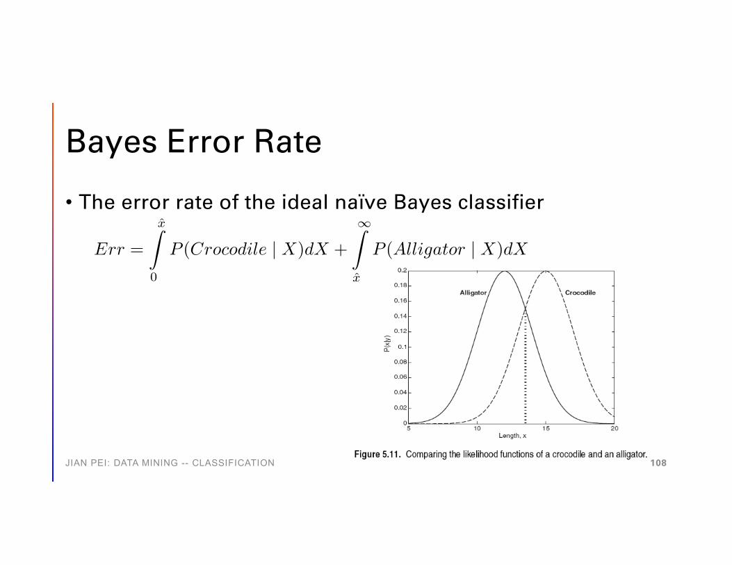
Bayes Error Rate

• The error rate of the ideal naïve Bayes classifier

Err =

x̂Z

0

P (Crocodile | X)dX +

1Z

x̂

P (Alligator | X)dX


Pros and Cons

• Pros• Easy to implement • Good results obtained in many cases

• Cons• A (too) strong assumption: independent attributes

• How to handle dependent/correlated attributes?• Bayesian belief networks


Instance-based Methods

• Instance-based learning• Store training examples and delay the processing until a new

instance must be classified (“lazy evaluation”)

• Typical approaches• K-nearest neighbor approach

• Instances represented as points in an Euclidean space• Locally weighted regression

• Construct local approximation• Case-based reasoning

• Use symbolic representations and knowledge-based inference


The K-Nearest Neighbor Method

• Instances are points in an n-D space• The k-nearest neighbors (KNN) in the Euclidean distance

• Return the most common value among the k training examples nearest to the query point

• Discrete-/real-valued target functions

. _

+_ xq

+

_ _+

_

_

+


KNN Methods

• For continuous-valued target functions, return the mean value of the k nearest neighbors

• Distance-weighted nearest neighbor algorithm• Give greater weights to closer neighbors

• Robust to noisy data by averaging k-nearest neighbors• Curse of dimensionality

• Distance could be dominated by irrelevant attributes• Axes stretch or elimination of the least relevant attributes

wd xq xi

º 12( , )


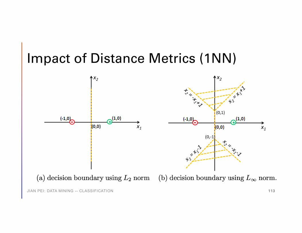
Impact of Distance Metrics (1NN)


Lazy vs. Eager Learning

• Efficiency: lazy learning uses less training time but more predicting time

• Accuracy• Lazy method effectively uses a richer hypothesis space• Eager: must commit to a single hypothesis that covers the entire

instance space


Decision Boundaries


(a) Decision Tree Classifier (b) 1Nearest-Neighbor Classifier (c) Linear Classifier

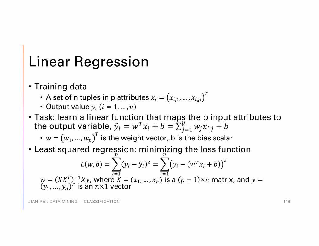
Linear Regression

• Training data• A set of n tuples in p attributes 𝑥𝑥! = 𝑥𝑥!,#, … , 𝑥𝑥!,$

%

• Output value 𝑦𝑦! 𝑖𝑖 = 1,… , 𝑛𝑛• Task: learn a linear function that maps the p input attributes to

the output variable, "𝑦𝑦! = 𝑤𝑤"𝑥𝑥! + 𝑏𝑏 = ∑#$%& 𝑤𝑤#𝑥𝑥!,# + 𝑏𝑏

• 𝑤𝑤 = 𝑤𝑤#, … ,𝑤𝑤$%

is the weight vector, b is the bias scalar

• Least squared regression: minimizing the loss function

𝐿𝐿 𝑤𝑤, 𝑏𝑏 =,!&#

'

𝑦𝑦! − .𝑦𝑦! ( =,!&#

'

𝑦𝑦! − 𝑤𝑤%𝑥𝑥! + 𝑏𝑏(

𝑤𝑤 = 𝑋𝑋𝑋𝑋% )#𝑋𝑋𝑦𝑦, where 𝑋𝑋 = (𝑥𝑥#, … , 𝑥𝑥') is a 𝑝𝑝 + 1 ×𝑛𝑛 matrix, and 𝑦𝑦 =𝑦𝑦#, … , 𝑦𝑦' % is an 𝑛𝑛×1 vector


Example


𝑤𝑤 =∑)*!" 𝑥𝑥)(𝐴𝐴) − 5𝐴𝐴)

∑)*!" 𝑥𝑥)+ −1𝑛𝑛 ∑)*!" 𝑥𝑥)

+

𝑏𝑏 =1𝑛𝑛A@A>

J

(𝑦𝑦@ − 𝑤𝑤𝑥𝑥@)

Perceptron

• To use linear regression for classification, let 𝑦𝑦! = 1 if the i-thtuple is in the positive class, and 𝑦𝑦! = 0 if it is in the negative class• Set "𝑦𝑦! = sign 𝑤𝑤"𝑥𝑥! , where 𝑠𝑠𝑠𝑠𝑠𝑠𝑠𝑠 𝑧𝑧 = 1 if 𝑧𝑧 > 0 and 𝑠𝑠𝑠𝑠𝑠𝑠𝑠𝑠 𝑧𝑧 = 0

otherwise• Training algorithm

• Start with a random assignment of w• For tuple 𝑥𝑥!,

• If (𝑦𝑦! = 𝑦𝑦_𝑖𝑖, do nothing• If (𝑦𝑦! ≠ 𝑦𝑦_𝑖𝑖, if 𝑦𝑦! = 1, 𝑤𝑤 ← 𝑤𝑤 + 𝜂𝜂𝑥𝑥!, otherwise 𝑦𝑦! = 0, 𝑤𝑤 ← 𝑤𝑤 − 𝜂𝜂𝑥𝑥!. 𝜂𝜂 > 0 learning

rate• Repeat until w converges or reaches the maximum number of iterations


Example


Sigmoid Function

• 𝜎𝜎 𝑧𝑧 = !!,-*+

= -+

!,-+, can be used to express the posterior

probability of observing a positive class label, that is, confidence

• 𝑇𝑇 :𝐴𝐴) = 1 𝑥𝑥) , 𝑤𝑤 = 𝜎𝜎 𝑤𝑤.𝑥𝑥) = !

!,-*,-./

• Equivalent to linear regressionpredict :𝐴𝐴) = 1 if 𝑤𝑤.𝑥𝑥) > 0


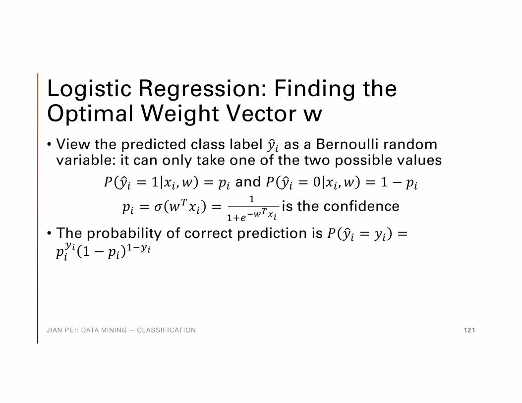
Logistic Regression: Finding the Optimal Weight Vector w• View the predicted class label :𝐴𝐴) as a Bernoulli random

variable: it can only take one of the two possible values𝑇𝑇 :𝐴𝐴) = 1 𝑥𝑥) , 𝑤𝑤 = 𝑝𝑝) and 𝑇𝑇 :𝐴𝐴) = 0 𝑥𝑥) , 𝑤𝑤 = 1 − 𝑝𝑝)

𝑝𝑝) = 𝜎𝜎 𝑤𝑤.𝑥𝑥) = !

!,-*,-./is the confidence

• The probability of correct prediction is 𝑇𝑇 :𝐴𝐴) = 𝐴𝐴) =𝑝𝑝)// 1 − 𝑝𝑝) !0//


Logistic Regress

• Objective: maximize the overall probability of correct prediction

𝑤𝑤∗ = argmax2𝐿𝐿 𝑤𝑤 = ∏)*!" 𝑇𝑇 :𝐴𝐴) = 𝐴𝐴) = ∏)*!

" 𝑝𝑝)// 1 − 𝑝𝑝) !0//

= ∏)*!" -,

-./

!,-*,-./

//!

!,-*,-./

!0//

• For convenience, take logarithm

𝑤𝑤∗ = argmax2𝑙𝑙 𝑤𝑤 = F)*!

"

𝐴𝐴)𝑥𝑥).𝑤𝑤 − log(1 + 𝑒𝑒2-3/)


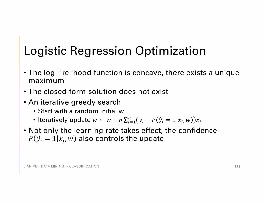
Logistic Regression Optimization

• The log likelihood function is concave, there exists a unique maximum

• The closed-form solution does not exist• An iterative greedy search

• Start with a random initial w• Iteratively update 𝑤𝑤 ← 𝑤𝑤 + 𝜂𝜂 ∑@A>

J 𝑦𝑦@ − 𝑃𝑃 C𝑦𝑦@ = 1 𝑥𝑥@ , 𝑤𝑤 𝑥𝑥@• Not only the learning rate takes effect, the confidence 𝑇𝑇 :𝐴𝐴) = 1 𝑥𝑥) , 𝑤𝑤 also controls the update


Logistic Regression

• If the training set is linearly separable, the algorithm may converge to a weight vector w with infinitely large norm

• Solution: introduce a regularization term 𝑤𝑤 + in the objective function

𝑤𝑤∗ = argmax2𝑙𝑙 𝑤𝑤 = ∑)*!" (𝐴𝐴)𝑥𝑥).𝑤𝑤 − log(1 + 𝑒𝑒2-3/)) − |𝑤𝑤|+

• Stochastic gradient descent: at each iteration, only use a small random sample to update


Linearly Separable


A2

A1

Class 1, y = +1

Class 2, y = −1

Maximum Separation


A1

A2

Large margin

A1

A2

Small margin

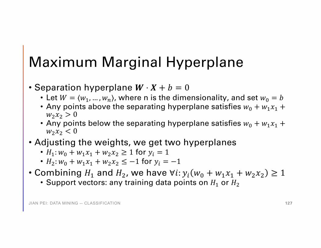
Maximum Marginal Hyperplane

• Separation hyperplane 𝑾𝑾 ⋅ 𝑿𝑿 + 𝑏𝑏 = 0• Let 𝑊𝑊 = ⟨𝑤𝑤>, … , 𝑤𝑤J⟩, where n is the dimensionality, and set 𝑤𝑤K = 𝑏𝑏• Any points above the separating hyperplane satisfies 𝑤𝑤K + 𝑤𝑤>𝑥𝑥> +𝑤𝑤B𝑥𝑥B > 0

• Any points below the separating hyperplane satisfies 𝑤𝑤K + 𝑤𝑤>𝑥𝑥> +𝑤𝑤B𝑥𝑥B < 0

• Adjusting the weights, we get two hyperplanes• 𝐻𝐻>: 𝑤𝑤K + 𝑤𝑤>𝑥𝑥> + 𝑤𝑤B𝑥𝑥B ≥ 1 for 𝑦𝑦@ = 1• 𝐻𝐻B: 𝑤𝑤K + 𝑤𝑤>𝑥𝑥> + 𝑤𝑤B𝑥𝑥B ≤ −1 for 𝑦𝑦@ = −1

• Combining 𝐻𝐻! and 𝐻𝐻+, we have ∀𝑖𝑖: 𝐴𝐴) 𝑤𝑤4 + 𝑤𝑤!𝑥𝑥! + 𝑤𝑤+𝑥𝑥+ ≥ 1• Support vectors: any training data points on 𝐻𝐻> or 𝐻𝐻B


Maximizing Separation Margin

• Margin size: +| 𝑾𝑾 |

, | 𝑾𝑾 | is the Euclidean norm of W

• Support vector machine (SVM) optimization problem

min 𝑾𝑾+

s.t. ∀𝑖𝑖: 𝐴𝐴) 𝑾𝑾𝑻𝑻𝑿𝑿) + 𝑏𝑏 ≥ 1


Non-linear SVM


• For linearly inseparable data, project the data to high dimensional space where it is linearly separable

-1 0 +1

+ +-

(1,0)(0,0)

(0,1) +

+-

General Steps in SVM

• Use a non-linear mapping to transform the original training data into a higher dimensional space

• Search for the linear optimal separating hyperplane


Associative Classification

• Mine association possible rules (PR) in form of condset à c• Condset: a set of attribute-value pairs• C: class label

• Build classifier• Organize rules according to decreasing precedence based on

confidence and support

• Classification• Use the first matching rule to classify an unknown case


Associative Classification Methods

• CBA (Classification By Association: Liu, Hsu & Ma, KDD’98)• Mine association possible rules in the form of

• Cond-set (a set of attribute-value pairs) à class label• Build classifier: Organize rules according to decreasing precedence

based on confidence and then support

• CMAR (Classification based on Multiple Association Rules: Li, Han, Pei, ICDM’01)

• Classification: Statistical analysis on multiple rules


Classification by Aggregating Emerging Patterns• Emerging pattern (EP): A pattern frequent in one class of

data but infrequent in others• Age<=30 is frequent in class “buys_computer=yes” and infrequent

in class “buys_computer=no”• Rule: age<=30 à buys computer

• G. Dong & J. Li. Efficient mining of emerging patterns: discovering trends and differences. In KDD’99


How to Mine Emerging Patterns?

• Border differential• Max-patterns in D1 w.r.t. min_sup=90%• Max-patterns in D2 w.r.t. min_sup=10%• X is a pattern covered by a max-pattern in D1 but not by a max-

pattern in D2 à X is an emerging pattern

• Method• Mine max-patterns in D1 and D2, respectively• Compare the two sets of borders, find the “maximal” patterns that

are frequent in D1 and infrequent D2


Using All Features or Some Features

• Not all features may be related to class labels• Feature selection: choosing some features that have good

correlation with class labels• Feature engineering: transforming the original features into

new features that are more effective in classification


Example

• Irrelevant attributes: A• Redundant attributes: B and D• Feature selection: B and C• Feature engineering: B + C


A B C D Class

0 1 8 3 Positive

1 7 2 10 Positive

1 1 2 2 Negative

0 2 1 3 Negative

Correlation with Classes

• 𝜒𝜒7 test for categorical attributes• Discretize a continuous attribute to conduct 𝜒𝜒( test

• Compute Fisher score between a continuous attribute and theclasses

𝑠𝑠 =∑#$%8 𝑠𝑠# 𝜇𝜇# − 𝜇𝜇

7

∑#$%8 𝑠𝑠#𝜎𝜎#7• c: the total number of classes• 𝑛𝑛0: the number of training samples in class j• 𝜇𝜇0 and 𝜎𝜎0(: the mean and variance of the attribute among all tuples that

belong to class j• 𝜇𝜇: the mean of the attribute


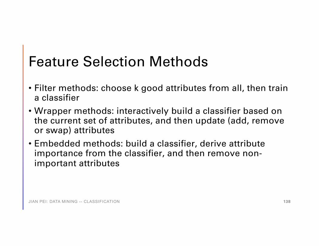
Feature Selection Methods

• Filter methods: choose k good attributes from all, then train a classifier

• Wrapper methods: interactively build a classifier based on the current set of attributes, and then update (add, remove or swap) attributes

• Embedded methods: build a classifier, derive attribute importance from the classifier, and then remove non-important attributes


Summary

• Classification: a two-step process• Decision trees• Classification performance evaluation• Ensemble methods• Bayesian methods and naïve Bayes• Lazy methods• Linear classifiers• Support vector machines (SVM)• Associative classification• Feature selection


Date post:	19-Mar-2022
Category:	Documents
Upload:	others
View:	3 times
Download:	0 times

Classification - Simon Fraser University

Documents