Classifying Ash Cloud Attributes of Eyjafjallajökull Volcano, Iceland, using Satellite Remote Sensing
by
Katrina Jane Gressett
A Thesis Presented to the
FACULTY OF THE USC DORNSIFE COLLEGE OF LETTERS, ARTS AND SCIENCES
University of Southern California
In Partial Fulfillment of the
Requirements for the Degree
MASTER OF SCIENCE
(GEOGRAPHIC INFORMATION SCIENCE AND TECHNOLOGY)
May 2021
Copyright © 2021 Katrina Jane Gressett
ii
To Mom and Dad, thank you for encouraging my curiosity.
To Reilly, Kaylee, and Juniper, thank you for knowing exactly when I needed to play.
iii
Acknowledgements
I am grateful to my mentor, Professor Fleming, for the direction I needed and my other faculty
advisors who assisted me when needed. I want to thank my manager, Dr. Cormode, for his
understanding and words of wisdom and my employer, Bay4 Technical Services, which allowed
me time away from the office to complete this work. I am grateful for the data provided to me by
the EARLINET Project and NASA.
iv
Table of Contents
Dedication ....................................................................................................................................... ii
Acknowledgements ........................................................................................................................ iii
List of Tables ................................................................................................................................ vii
List of Figures .............................................................................................................................. viii
Abbreviations .................................................................................................................................. x
Abstract ......................................................................................................................................... xii
Chapter 1 Introduction .................................................................................................................... 1
1.1. Study Objectives .................................................................................................................1
1.2. Motivation ...........................................................................................................................2
1.2.1. Volcanic Health Hazards ...........................................................................................2
1.2.2 Ash Cloud Forecasts ...................................................................................................3
1.3. Study Area ..........................................................................................................................5
Chapter 2 Literature Review ........................................................................................................... 8
2.1. Remote Sensing of Volcanic Ash .......................................................................................8
2.1.1. MODIS Instrument Package ....................................................................................10
2.1.2. InSAR Remote Sensing ...........................................................................................10
2.2. Ground-Based LiDAR ......................................................................................................11
2.3. Eruption Cloud Forecasting ..............................................................................................11
2.4. Volcanic Effects on Aircraft .............................................................................................13
Chapter 3 Methods ........................................................................................................................ 15
3.1. Data Sources .....................................................................................................................15
3.1.1. EARLINET Data .....................................................................................................17
3.1.2. MODIS Data ............................................................................................................18
3.2. EARLINET Processing Overview ....................................................................................19
v
3.2.1. Database Manipulation ............................................................................................20
3.2.2. Daily Interpolations .................................................................................................21
3.2.3. Interpolations Tested ................................................................................................21
3.2.4. Inverse Distance Weighting .....................................................................................24
3.2.5. Cross-Validation ......................................................................................................25
3.3. MODIS Processing Overview...........................................................................................26
3.3.1. MODIS Data Import and Corrections ......................................................................28
3.3.2. Radiance Values.......................................................................................................28
3.3.3. Image Mosaic ...........................................................................................................30
3.3.4. Brightness Temperature ...........................................................................................31
3.3.5. Ash Cloud Classification .........................................................................................31
3.4. Flight Path Proximity ........................................................................................................32
Chapter 4 Results .......................................................................................................................... 34
4.1. EARLINET Interpolation .................................................................................................34
4.2. MODIS Brightness Temperature Difference ....................................................................41
4.3. Flight Paths .......................................................................................................................48
Chapter 5 Discussion .................................................................................................................... 50
5.1. Discussion .........................................................................................................................50
5.2. Limitations ........................................................................................................................51
5.2.1. EARLINET Interpolations .......................................................................................51
5.2.2. MODIS and BTD .....................................................................................................52
5.3. Future Research ................................................................................................................53
5.3.1. Ash Cloud Thickness ...............................................................................................53
5.3.2. Eruptive Volume ......................................................................................................53
5.3.3. Ash Cloud Density Contours ...................................................................................54
vi
5.4. Conclusions .......................................................................................................................54
References ..................................................................................................................................... 56
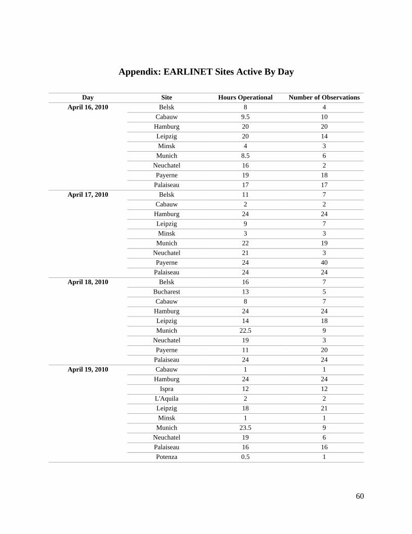
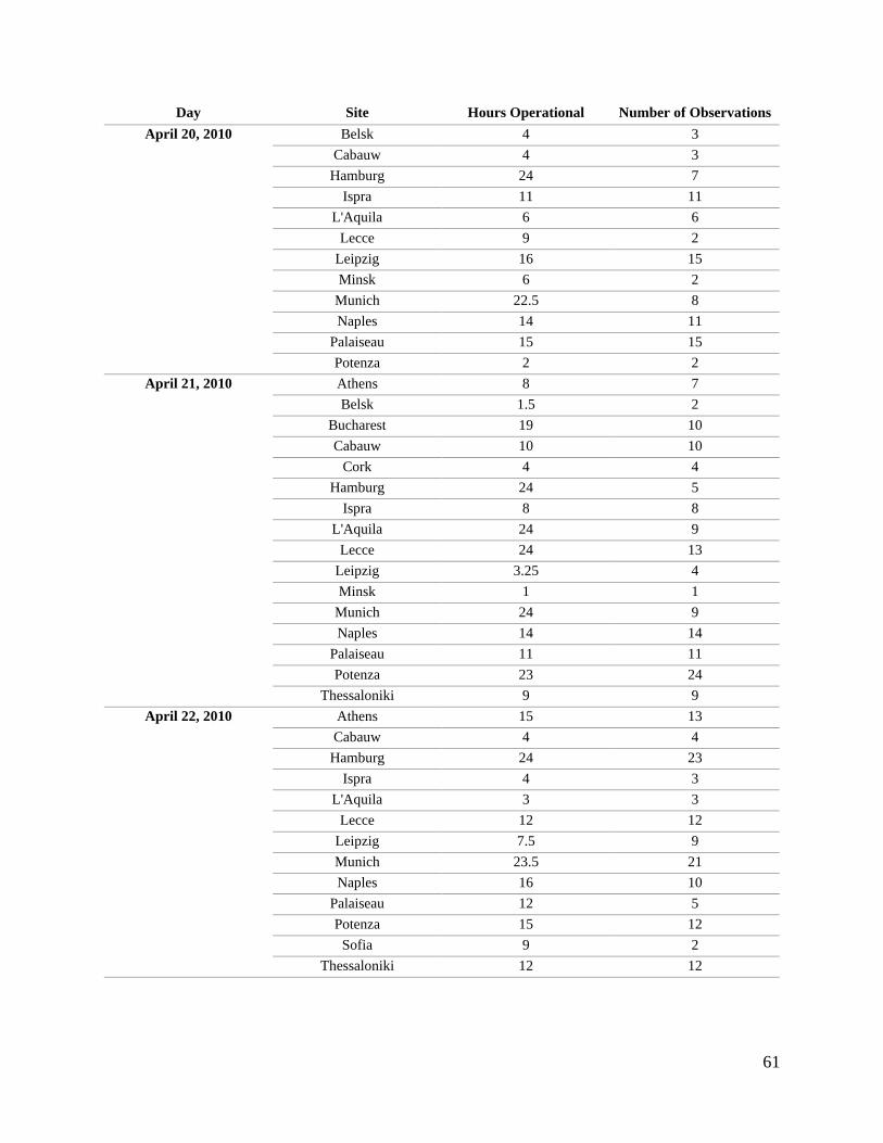
Appendix: EARLINET Sites Active By Day ............................................................................... 60
vii
List of Tables
Table 1. Data used in this project.................................................................................................. 16
Table 2. Radiance scale and offset values provided by NASA for each of the three bands used in
this project. .................................................................................................................................... 29
viii
List of Figures
Figure 1. The volcanic ash advisory forecast for April 15 until April 16, 2010. ............................ 4
Figure 2. The study area showing Iceland, central European counties, and the location of the
Eyjafjallajökull volcano. ................................................................................................................. 6
Figure 3. Time snapshots of ash mass loading produced by the WRF-Chem model reproduced
from Webley et al. (2012). ............................................................................................................ 13
Figure 4. The EARLINET stations used in this project. ............................................................... 18
Figure 5. The workflow for processing EARLINET data. ........................................................... 20
Figure 6. The left image displays the RBF with Spline interpolation, while the right displays the
IDW interpolation. ........................................................................................................................ 23
Figure 7. The results of the kriging interpolation. ........................................................................ 24
Figure 8. The workflow for the MODIS data. .............................................................................. 27
Figure 9. IDW interpolation for April 16, 2010............................................................................ 37
Figure 10. IDW interpolation for April 17, 2010. ......................................................................... 37
Figure 11. IDW interpolation for April 18, 2010. ......................................................................... 38
Figure 12. IDW interpolation for April 19, 2010. ......................................................................... 38
Figure 13. IDW interpolation for April 20, 2010. ......................................................................... 39
Figure 14. IDW interpolation for April 21, 2010. ......................................................................... 39
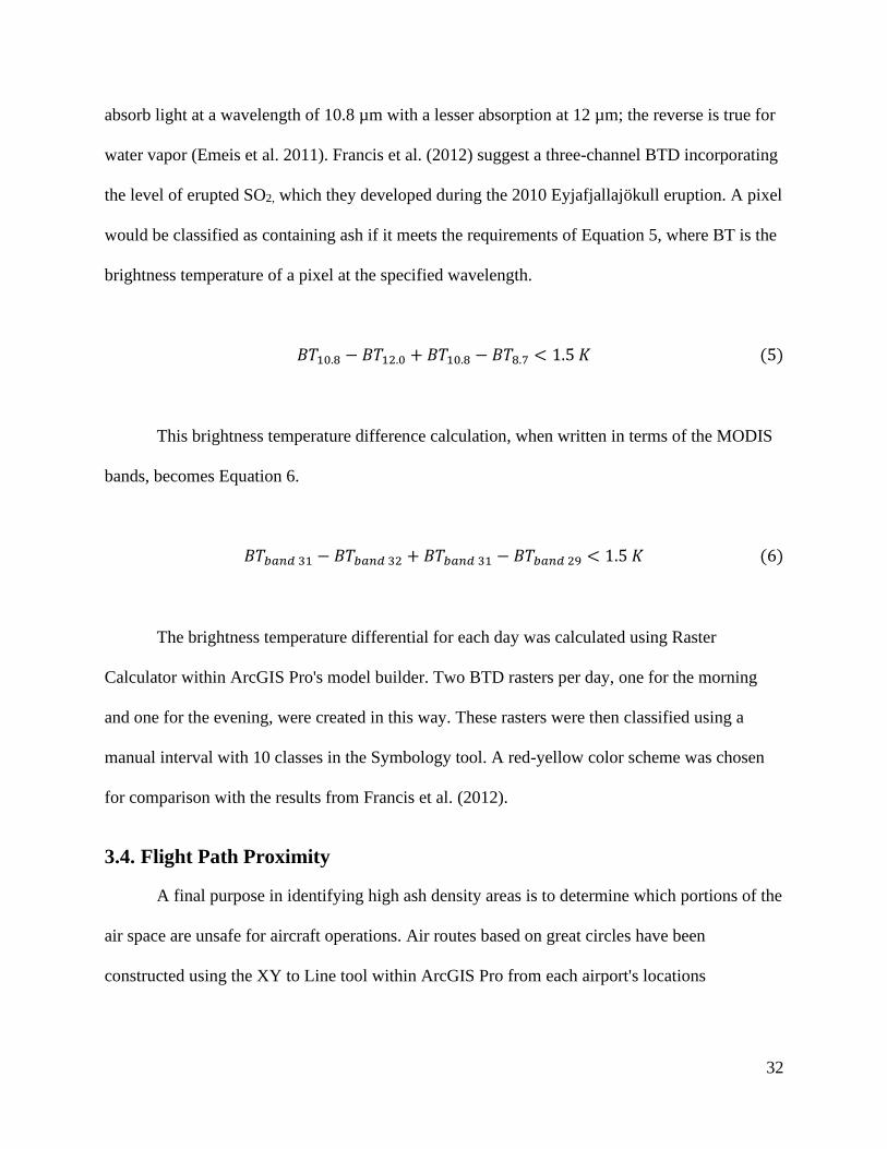
Figure 15. IDW interpolation for April 22, 2010. ......................................................................... 40
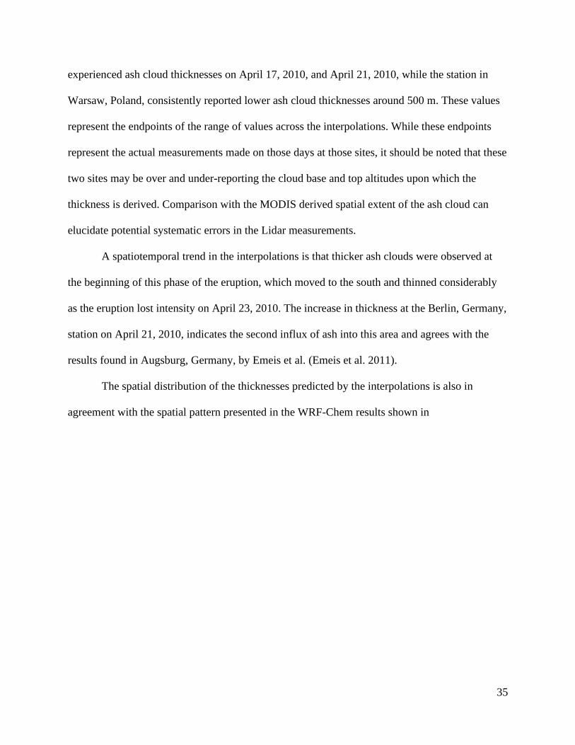
Figure 16. IDW interpolation for April 23, 2010. ......................................................................... 40
Figure 17. IDW interpolation for April 24, 2010. ......................................................................... 41
Figure 18. Brightness Temperature Difference for the morning of April 17, 2010. ..................... 44
ix
Figure 19. Brightness Temperature Difference for the evening of April 17, 2010. ..................... 44
Figure 20. Brightness Temperature Difference for the morning of April 21, 2010. ..................... 45
Figure 21. Brightness Temperature Difference for the morning of April 21, 2010. ..................... 45
Figure 22. BTD for the morning of April 17, 2020, zoomed in for comparison purposes. .......... 46
Figure 23. NASA MODIS color composite for the morning of April 17, 2010. .......................... 46
Figure 24. Brightness Temperature Difference for the evening of April 17, 2010. ..................... 47
Figure 25. Ash cloud classifications from the SEVIRI instrument, from Gudmundsson et al. 2012
....................................................................................................................................................... 47
Figure 26. Air routes across Europe along with the BTD ash signal on the morning of April 17,
2010............................................................................................................................................... 49
x
Abbreviations
AOT Aerosol Optical Thickness
AVHRR Advanced Very High-Resolution Radiometer
BTD Brightness Temperature Difference
CALIPSO Cloud-Aerosol LiDAR and Infrared Pathfinder Satellite Observations
COPD Chronic Obstructive Pulmonary Disorder
DN Digital Number
EARLINET European Aerosol Research LiDAR Network
GIS Geographic information system
GISci Geographic information science
IDW Inverse Distance Weighted
IASI Infrared Atmospheric Sounding Interferometer
InSAR Interferometric Synthetic Aperature Radar
LiDAR Light Detection and Ranging
RBF Radial Basis Function
RMSE Root-Mean-Square Error
SEVIRI Spinning Enhanced Visible and Infrared Imager
SO2 Sulfuric Dioxide
SSI Spatial Sciences Institute
TOA Top of Atmosphere
USC University of Southern California
VAA Volcanic Ash Advisory
VAAC Volcanic Ash Advisory Centers
xi
VEI Volcanic Explosivity Index
WRF-Chem Weather Research and Forecasting In-line Chemistry
xii
Abstract
Tracking volcanic ash clouds is integral to ensuring the safety of people traveling by air and
living on the ground. The explosive eruption of Eyjafjallajökull volcano, Iceland, that began on
April 14, 2010, produced a column of steam and ash carried by the jet stream to Europe. In
London, the volcanic Ash Advisory Center provided the ash cloud's overall spatial extent across
Europe but was unable to provide localized forecasts or details such as cloud density. This
eruption forced the most prolonged suspension of air travel in Europe since the second world war
with significant cost to airlines and travelers.
High temporal, multispectral thermal satellite imagery from the MODIS instrument
provides a platform for tracking eruptive materials. This study uses the brightness temperature
difference between MODIS thermal bands to track the ash cloud for each day of the eruption.
Unsupervised classification is used to determine the spatial extent of the ash cloud.
Measurements from the ground-based EARLINET Lidar network are used to compare the results
derived from MODIS imagery. Interpolations based on the EARLINET Lidar data are
comparable to the MODIS classification but may not be economical for developing regions.
1
Chapter 1 Introduction
Volcanic eruptions produce many risks to human populations, including operational and safety
issues for air traffic. The 2010 eruption of Eyjafjallajökull volcano, Iceland, was an explosive
Plinian style eruption that produced an eruptive ash column reaching heights of 8 – 10 km as
measured by a weather radar station in Iceland (Gudmundsson et al. 2012; Gasteiger et al. 2011;
Langmann et al. 2012). These types of eruptions constitute a source of risk for air travel as fine
ash particles can re-melt inside jet engines and cause engine failure. An example of this occurred
during the 1989 – 1990 eruption of Mount Redoubt when KLM flight 867 had all four engines
disabled after encountering the ash cloud (Casadevall 1994). The eruptive volume of the ash
plume must be calculated along with the density of ash particles to forecast the risk to air traffic,
yet this can be a computationally challenging undertaking (Webley et al. 2012; 2013).
The 2010 eruption of Eyjafjallajökull volcano was modest, with a volcanic explosivity
index (VEI) of 6, yet it caused significant disruption to air travel across Europe over the 14th –
25th of April 2010 (Ulfarsson and Unger 2011). Generating daily estimates of the ash cloud's
spatial extent can help direct emergency response and reroute flight paths to avoid the ash cloud's
high-density areas. Both ground-based and satellite remote sensing methods can generate these
estimates but may not have availability in all parts of the world or for all events. Further,
countries with limited funding may be only able to invest in one remote sensing method. A
comparison of these methods can be an essential tool in choosing where to place limited funds.
1.1. Study Objectives
The research objective of this thesis is to determine how well an interpolation of sparse,
ground-based LiDAR measurements can estimate the spatial distribution of the ash cloud
released during the 2010 Eyjafjallajökull volcano eruption compared to thermal satellite imagery
2
using the MODIS instrument on the Aqua and Terra satellites for use in determining air space
restrictions.
1.2. Motivation
This work's motivation is to provide insight to the airlines and emergency response
managers during volcanic eruptions. During the Eyjafjallajökull eruption, air traffic over Europe
was suspended for six days at a considerable economic cost to airlines and travelers. Ulfarsson
and Unger (2011) suggest that the last time Europe has seen such a disruption of air travel was
during World War II. Ash cloud densities must be below 200 µg/m3 for aircraft to travel safely
through them (Ulfarsson and Unger 2011). A contoured ash thickness map would indicate which
air routes, if any, had the potential to remain safely open.
1.2.1. Volcanic Health Hazards
Fine volcanic ash particles and sulfur dioxide (SO2), even at lower concentrations, pose a
health risk to people. Volcanic ash is pyroclastic material 2 mm or smaller in diameter, and fine
volcanic ash is much smaller, less than around 15 µm (Horwell and Baxter 2006). Newly erupted
ash has jagged edges and may be coated in condensed acids formed from the mixing of gasses
such as SO2 and water. These particles can irritate the eyes and airways, even of healthy people.
According to Horwell and Baxter (2006), ash this size or smaller can cause ailments such as
laryngitis, bronchitis, asthma, chronic obstructive pulmonary disorder (COPD), cancer, and
silicosis.
The eruption of sulfur dioxide can also pose direct health risks. When SO2 mixes with
water vapor in the atmosphere, it can form sulfuric acid (H2SO4), among other sulfate
compounds. Sulfuric acid is a strong acid and can be particularly damaging to the eyes and lungs.
3
When a gas cloud of SO2 is near the ground, as often occurs on Mount Kilauea in Hawaii, it is
known as vog or volcanic smog (Tam et al. 2016). Even when erupted higher into the
atmosphere, SO2 can still pose a threat to people if aircraft fly through a cloud of this gas. The
SO2 can be drawn into an aircraft with other air through the passenger air handling systems
causing respiratory distress.
Sulfur dioxide poses an indirect health risk when erupted high into the atmosphere. When
SO2 has erupted into the lower stratosphere, it decomposes into sulfuric acid (H2SO4), which
reflects and absorbs incoming solar radiation increasing the albedo of the planet. When the
amount of SO2 released from volcanoes are large enough, average global temperatures drop
(Ward 2009). Ward (2009) reports that in the three years after the large Mount Pinatubo,
Philippines, 1991 eruption (VEI 6), which injected up to 19 megatons of SO2, global average
temperatures dropped by as much as 0.5 °C. Similarly, global average temperatures dropped by
as much as 0.7 °C after the 1815 eruption of Mount Tambora (Stothers 1984). This eruption was
responsible for causing "the year without a summer" in the Northern Hemisphere in 1816,
leading to crop failure and famine.
1.2.2 Ash Cloud Forecasts
The Volcanic Ash Advisory Center (VAAC) is responsible for issuing advisories on
volcanic ash clouds that may endanger aircraft. The VAAC has nine district offices around the
world, including one in London. These offices monitor volcanic eruptions within their districts
using satellite imagery, radar, Lidar, and sun photometers to detect and track volcanic ash and
other erupted aerosols (Christopher et al. 2012).
Forecasters use meteorological data and attributes of the volcanic eruption, such as plume
height and ash particle size, in the NAME dispersion model to generate a forecast for ash cloud
4
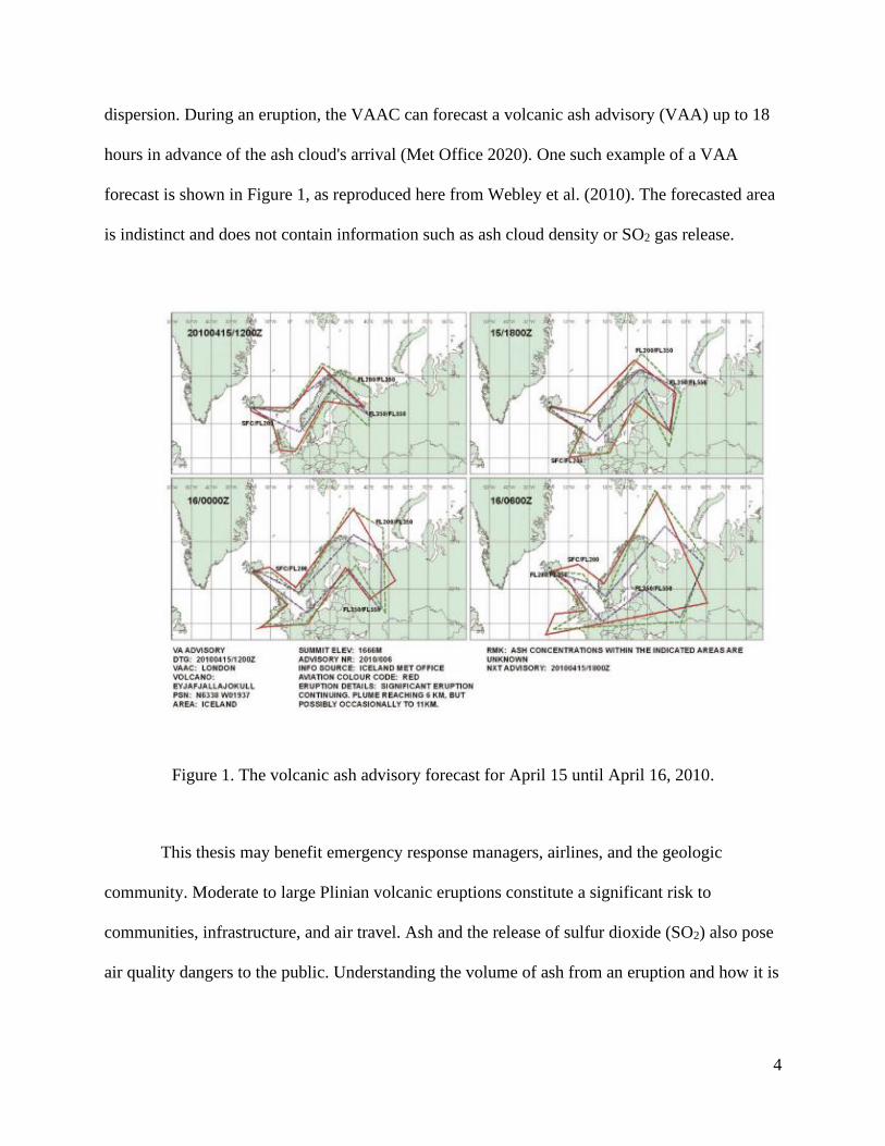
dispersion. During an eruption, the VAAC can forecast a volcanic ash advisory (VAA) up to 18
hours in advance of the ash cloud's arrival (Met Office 2020). One such example of a VAA
forecast is shown in Figure 1, as reproduced here from Webley et al. (2010). The forecasted area
is indistinct and does not contain information such as ash cloud density or SO2 gas release.
Figure 1. The volcanic ash advisory forecast for April 15 until April 16, 2010.
This thesis may benefit emergency response managers, airlines, and the geologic
community. Moderate to large Plinian volcanic eruptions constitute a significant risk to
communities, infrastructure, and air travel. Ash and the release of sulfur dioxide (SO2) also pose
air quality dangers to the public. Understanding the volume of ash from an eruption and how it is
5
dispersed can guide evacuations and suspension of air travel. Rapid monitoring via remote
sensing can provide the guidance needed for these responses.
1.3. Study Area
Situated just east of the mid-Atlantic rift and 77 miles southeast of Iceland's capital,
Reykjavik, along Iceland's southern coast, lies Eyjafjallajökull volcano, Iceland, a glacier-
covered volcano capable of explosive volcanic eruptions(Francis 1989; Prata 1989). Directly to
the east lies the more substantial Katla Volcano. This project's study area, shown in Figure 2,
encompasses the Northeast Atlantic, the North Sea, Northern Europe, and the Iberian Peninsula.
When the eruptive column reached the polar jet stream's altitude, ash blew into this study area
(CIA 2020).
Iceland is a small island country with an area of 103,000 km2 and a population estimated
at 350,000 in 2020 (BBC News 2010). The largest city and capital, Reykjavik, has a population
of 122,853 people as of 2016. Half of the entire island population is estimated to live in the area
surrounding the capital (Hall et al. 2015). The remaining population lives along the coastline.
The island was formed primarily formed from volcanic processes. The island is situated
atop a mantle plume, also known as a hot spot. A hot spot brings significant volumes of mantle
material to Earth's crust, that can melt and eventually erupt (Gudmundsson et al. 2012). The
divergent tectonic plate boundary formed by the mid-Atlantic rift transects the island from the
southwest, near Reykjavik, across to the northeast. The island has 32 volcanoes. Of these, 18
have been active since human settlement began in the area over 900 years ago (NASA 2020;
Jenner 2017).
6
Figure 2. The study area showing Iceland, central European counties, and the location of the
Eyjafjallajökull volcano.
The magmatic provenance is primarily composed of mafic magma with similar effusive
eruptions, such as those found in Hawaii. However, explosive eruptions are not uncommon for
Icelandic volcanoes. Thordarson and Höskuldsson (2008) point out that Iceland has produced
some of the largest explosive eruptions to affect continental Europe. Many of Iceland's
7
volcanoes, including Eyjafjallajökull, are covered with glaciers. These thick blankets of ice can
cause even effusive eruptions to become explosive, steam-driven, phreatic eruptions when lava
causes the ice to flash into steam.
The explosive phase of the Eyjafjallajökull eruption, which began on April 14, 2010,
formed in the crater directly under the glacier bearing the same name (Sigmundsson et al. 2010;
Pedersen and Sigmundsson 2004). Meltwater flooded nearby rivers in the form of a jökulhlaup
and forced the evacuation of 800 people (Langmann et al. 2012; Francis 1989; Francis and
Rothery 2000). The meltwater mixed with the erupting magma to create an explosive style
eruption.
The North Atlantic Polar Jet Stream is a current of fast-moving air circumnavigating the
polar regions at the top of the troposphere, at an altitude between 7-12 km (Christopher et al.
2012; Francis, Cooke, and Saunders 2012). This current of air flows from west to east in an
undulating pattern near 60°N latitude. The Eyjafjallajökull ash cloud was transported by the
polar jet stream when it rose to altitudes of 8-10 km (Jenner 2017).
8
Chapter 2 Literature Review
The following sections explore different remote sensing techniques for observing volcanic ash
clouds, the current state of dispersion forecasts, and the effects of ash and sulfur dioxide on
aircraft and at ground level. A significant volume of work has been written about the 2010
eruption of the Eyjafjallajökull volcano. Specific case studies of remote sensing techniques,
forecast modeling, and ground-based Lidar are examined here and form the basis for the methods
used in this study.
2.1. Remote Sensing of Volcanic Ash
Remote sensing of volcanic ash clouds is an essential tool for assessing the hazards posed
by an eruption. Remote sensing of ash clouds can refer to several different technologies.
Multispectral imagery is widely used for ash cloud detection (Maccherone and Frazier 2014).
Satellite missions such as Landsat 8, Terra, and the Advanced Very High-Resolution Radiometer
(AVHRR), among others, provide moderate to high-resolution imagery in a wide range of
spectral bands with data freely available to the public (Massonnet and Feigl 1998).
Satellite and ground-based Light Detection and Ranging (LiDAR) instruments use laser
backscatter data to detect aerosols such as ash clouds. The Cloud-Aerosol Lidar and Infrared
Pathfinder Satellite Observations (CALIPSO) instrument provides spaceborne LiDAR data while
the European Aerosol Research LiDAR Network (EARLINET) is a ground-mounted LiDAR
network providing LiDAR backscatters for Europe. Multispectral imaging and LiDAR both
represent direct observation methods.
The final remote sensing technology is Interferometric Synthetic Aperture Radar
(InSAR). While InSAR is not used to directly sense volcanic eruptions, it can be used to
9
determine the total volume of a volcanic eruption when paired with geodetic techniques
(Sigmundsson et al. 2010).
Remote sensing methods using satellites have been regarded as the best tools for tracking
volcanic ash plumes since the 1990s (Jenner 2017). Volcanic ash is primarily composed of
silicate particles (SiO2) ranging in size from 0.1 µm to 1.2 µm (Maccherone and Frazier 2014).
Prata (1989) used the radiative transfer model to show that ash particles increasingly absorb
infrared radiation between 10 µm and 13 µm. and absorb infrared light more strongly at 12 µm
than at 10.8 µm. Prata (1989) chose these wavelengths as they correspond to the midpoint of the
thermal bands 4 and 5 of the AVHRR, which also encompass the 10 µm to 13 µm range
determined from the radiative transfer function. Prata (1989) additionally observed that this
increasing absorption by ash particles was the opposite pattern of absorption occurring in water
particles. When the brightness temperature difference (BTD) is calculated between these two
wavelengths, ash particles produce a strongly negative value, and water particles produce
positive values. In this way, ash clouds are distinguished from water clouds.
Building on Prata's 1989 work, Francis et al. (2012) test four classification variations
using two and three-channel BTD but using the Spinning Enhanced Visible and Infrared Imager
(SEVIRI) instrument. For the Eyjafjallajökull eruption, Francis et al. (2012) test the difference
between 10.8 µm and 12 µm with the incorporation of a difference term at 8.7 µm, suggesting
that as Sulfur dioxide (SO2) has a strong absorption at this wavelength, the resultant delineation
of the ash cloud from water cloud is more pronounced. Dubuisson et al. (2014) confirm that BTD
is the standard ash cloud classification in their work comparing SEVIRI, MODIS, and IASI
(Infrared Atmospheric Sounding Interferometer) data for the portion of the Eyjafjallajökull
eruption occurring on May 6 2010; a date chosen as data from all three instruments is available.
10
2.1.1. MODIS Instrument Package
Volcanic eruptions occurring over multiple days are best studied with satellite
instruments that have a high temporal resolution. The Moderate Resolution Imaging
Spectroradiometer (MODIS), launched in 1999 on the Terra and Aqua satellites, provides high
spatial and temporal resolution. The purpose of the MODIS mission is to image every point of
Earth every 1-2 days in 36 bands with bands 20 – 36 devoted to near- and mid-infrared
wavelengths specific to atmospheric studies (Massonnet and Feigl 1998). The MODIS
instrument's spatial resolution ranges from 250 m to 1 km, making it ideal for regional
atmospheric studies. Each MODIS image consists of a 5-minute orbital swath and a maximum
scan width of 2,330 km. The instrument can collect data in the emissive bands 20 – 36 at any
time (Sigmundsson et al. 2010).
2.1.2. InSAR Remote Sensing
Interferometric Synthetic Aperature Radar uses the difference in the phase of the waves
of two Synthetic Aperature Radar images separated by a time interval of days to years. The
resulting interferogram can be used to measure the deformation of Earth's crust at the millimeter
level (Amato et al. 2019). In this method, a volumetric change in the volcano itself is determined
using continuous GPS measurements on and around the volcano alongside the spatial extent of
deformation inferred from the InSAR data (Amato et al. 2019; Langmann et al. 2012; Wiegner et
al. 2012). The volcano must be observed before and after the eruption with pre-and post-eruption
volumes calculated. The eruptive volume is the difference in the pre and post-eruption volumes.
While a robust estimation of the eruptive volume can be achieved, it comes at the cost of
requiring a significant amount of time to generate. This method is not suitable for forecasting
11
risks of eruptive ash clouds, even though several forecast models need accurate eruptive volume
estimates.
2.2. Ground-Based LiDAR
The European Aerosol Research LiDAR Network (EARLINET) is a network of 31
ground-based LiDAR stations distributed across Europe in operation since 2000. The goal of
EARLINET is to continuously monitor aerosols in three dimensions (Amato et al. 2019). The
processed data consist of aerosol extinction values, backscattered LiDAR detections, and particle
depolarization ratios
EARLINET backscatter data is available in three wavelengths at 355 nm, 532 nm, and
1064 nm (Webley et al. 2012). Wiegner et al. (2012) suggest that the backscatter signal for the
Eyjafjallajökull ash-cloud is strongest at 1064 nm. Stations within EARLINET usually make
measurements every few days. In anticipation of the arrival of the ash-cloud from
Eyjafjallajökull, the measurement cadence increased to once per hour (Maccherone and Frazier
2014).
The spatial extent of the 2010 Eyjafjallajökull ash plume measured across this network
provides a comparison to previously mentioned remote sensing methods as well as the satellite-
based CALIPSO LiDAR instrument (Langmann et al. 2012; Wiegner et al. 2012). Webley et al.
(2012) use time-height cross-section data from the EARLINET as a comparison for the Weather
Research Forecast coupled with Chemistry (WRF-Chem) model and found some agreement
between the model and the EARLINET observations.
2.3. Eruption Cloud Forecasting
Forecasting an ash cloud's dispersal within hours to days is vital to the aviation
community and to governmental agencies responsible for mitigating hazards such as sulfur
12
dioxide and ash posed by volcanic eruptions. Forecasts, in the form of volcanic ash advisories,
are released by Volcanic Ash Advisory Centers (VAAC) around the world (Prata 1989;
Dubuisson et al. 2014; Francis, Cooke, and Saunders 2012). There are many ash- cloud
dispersion models, such as the Weather Research and Forecasting In-line Chemistry model
(WRF-Chem).
These models are similar in that they require numerical weather prediction alongside ash-
plume height and particle size distribution. Webley et al. (2012) also suggest that it is essential to
estimate accurately the eruptive mass, such as can be calculated from the eruptive volume.
Another distinctive feature of forecast models is the need for significant computing power.
Webley et al. (2012) report a requirement of 96 CPU-cores to achieve model run times under
half an hour.
The ash-cloud forecast maps, shown in Figure 1, released by the London VAAC and
reported in Webley et al. (2012) for April 14 and 15, 2010, are jagged, Europe-sized areas. These
forecast maps do not provide information on areas of high or low particle density. While general
warnings about air pollution based on these forecasts can be released to the public, areas of
heightened risk due to a higher density of ash particles may not be adequately warned.
Out of well-placed caution, aviation authorities used these forecasts to suspend air-travel
across Europe. The WRF-Chem model results shown in Figure 3 indicate that some portions of
the airspace had the potential to remain in service, particularly in Britain and Southern Europe on
April 16-17, 2010 (Webley et al. 2012).
13
Figure 3. Time snapshots of ash mass loading produced by the WRF-Chem model reproduced
from Webley et al. (2012).
2.4. Volcanic Effects on Aircraft
Aircraft, regarded as a safe form of travel, are susceptible to the fine ash and SO2 gas
erupted by volcanoes. The jet engines of modern aircraft operate at temperatures that can reach
1,200 – 2,000 °C. These temperatures are hot enough that volcanic ash entering the engine's
front can re-melt and stick to surfaces within the engine (Song et al. 2016). Jet engines consist of
many turbofans rotating at high speed in different directions. Molten ash on even one of these
parts can cause it to be unable to turn. Song et al. (2016) also point out that molten ash can clog
fuel injector nozzles. These effects result in the engine failing. When enough engines fail, the
result is a catastrophe.
14
Engine failure is not the only dangerous effect aircraft face from volcanic eruptions. The
1989-1990 eruption of the Redoubt volcano in Alaska affected seven flights that ranged from
Anchorage, Alaska, to west Texas (Casadevall 1994; Casadevall, Delos Reyes, and Schneider
1996). Newly erupted volcanic ash is slightly electrically charged and often contains condensed
sulfuric acid. According to Casadevall (1994), one plane encountered electromagnetic effects in
the form of St. Elmo's Fire from ash accumulating on the plane. The same plane experienced
pitting of the windscreen and leading edges. While the plane could make a safe landing and no
parts required replacing, KLM Flight 867 was not as fortunate. Casedevall (1994) describes that
this flight not only lost all four engines, eventually regaining two, but that the cabin of the
aircraft filled with smoke and sulfurous gasses from the eruption. After landing, it was
discovered that ash had been able to penetrate the plane's baggage and habitable areas and that
the air handling filters had been overwhelmed with ash. The aircraft's exterior, including all
windows and flight control surfaces, had been extensively damaged by abrasive ash particles.
The flight landed in Anchorage with no fatalities (Casadevall 1994).
15
Chapter 3 Methods
This chapter outlines the sources of data and methods that were used for this study. The first
section describes the satellite remote sensing products used. A description of the LiDAR
interpolation, along with the methodology of comparison to MODIS imagery, is provided.
Finally, the last section describes how the airline route data compares with the remote sensing
data to generate a list of affected airports and routes.
3.1. Data Sources
Data for this project come mainly from NASA's MODIS instrument on the Terra satellite,
the ground-based EARLINET Lidar network, and the Openflights.org website. These three
sources are described in Table 1.
16
Table 1. Data used in this project.
Data Set Source Description Purpose Data Type Bands Spatial
Resolution
Temporal
Resolution
Size on
Disk
Availability
MODIS
Satellite
Remote
Sensing Data
NASA MODIS
Terra and Aqua
Imagery
MODIS Level
1B Calibrated
Radiances for
all 36 MODIS
bands 1 km
resolution
The primary
data product
used to
calculate
eruptive
volumes,
densities, and
spatial extent
of the
eruption
GeoTiff
Raster files
29: 8.4 -8.7µm
31: 10.8 – 11.3µm
32: 11.7 – 12.3µm
1 km 1 / day 47 GB This data is freely
available for
download at
https://ladsweb.m
odaps.eosdis.nasa.
gov/missions-and-
measurements/scie
nce-
domain/modis-
L0L1/
Global Flight
Paths
Openflights.org Origin and
destination
airport locations
used to generate
a flight path
based on great
circles
This data is
necessary to
determine
which flight
paths would
be affected by
the ash cloud
Point data
in CSV
format
N/A N/A <1 GB This data is freely
available at
https://openflights.
org/
Terrestrial
LiDAR Data
European
Aerosol
Research LIDAR
Network
Database of the
horizontal,
vertical, and
temporal
distribution of
aerosols across
Europe
The satellite
remote
sensing-based
particle
densities
compared
with ground-
based
particulate
measurement
Database
of point
altitudes
describing
base and
top cloud
height
1/hour <1 GB This data is
available at
https://www.earlin
et.org/index.php?i
d=125
17
3.1.1. EARLINET Data
The European Aerosol Research Lidar Network (EARLINET) was established in 2000 to
study aerosol climatology. Originally a partnership between 19 universities located amongst 11
countries, the network has grown to include more than 30 instruments (Amato et al. 2019;
Madonna et al. 2015). Instruments participating in EARLINET collect data in three wavelengths
comprised of an ultraviolet wavelength at 351 nm, a green wavelength at 532 nm, and a thermal
wavelength at 1064 nm. Both ceilometers and multiwavelength Raman Lidars are used within
the network to produce Raman Backscatter profiles of the atmosphere above the instrument.
While each instrument can collect data in a near-continuous timeframe, in usual conditions, each
station often operates for about 1 hour each week (Amato et al. 2019; Madonna et al. 2015).
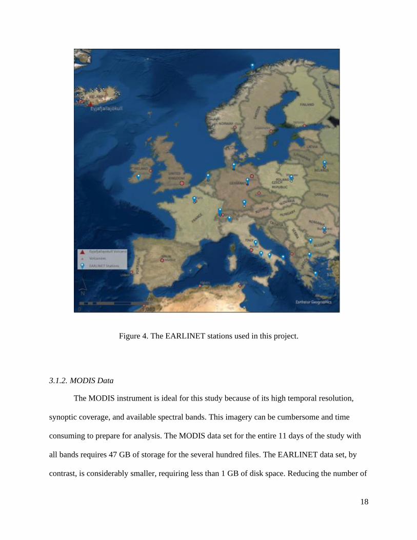
The EARLINET project provides specially prepared datasets for atmospheric events such
as the 2010 Eyjafjallajökull eruption. These analyzed data products are available in the form of a
database with tables indicating which stations were included in the analysis with the dates, times,
and location of observations; the Raman backscatter values with the wavelengths used in the
analysis; and the altitudes of the base, top, and center of mass of the volcanic cloud. This
database contained data from 24 stations throughout Europe, shown in Figure 4, which operated
between April 15, 2010, and May 26, 2010. Nineteen of the stations operated between April 15,
2010, and April 26, 2010. The data capture at some stations such as Hamburg, Germany, was
nearly continuous, with measurements occurring over one-hour time intervals for over twelve
hours a day. Many stations operated for only a few hours each day, while others had irregular
time intervals.
18
Figure 4. The EARLINET stations used in this project.
3.1.2. MODIS Data
The MODIS instrument is ideal for this study because of its high temporal resolution,
synoptic coverage, and available spectral bands. This imagery can be cumbersome and time
consuming to prepare for analysis. The MODIS data set for the entire 11 days of the study with
all bands requires 47 GB of storage for the several hundred files. The EARLINET data set, by
contrast, is considerably smaller, requiring less than 1 GB of disk space. Reducing the number of
19
days of satellite imagery examined and the number of bands included reduces both the disk space
requirements and the processing time required for the MODIS data.
Three days of MODIS data were chosen at the beginning, middle, and end of the eruptive
period to match the dates of measurements made by the EARLINET LiDAR network. These
dates were April 17, 2010, April 21, 2010, and April 24, 2010. Each of these days had 6-8 scenes
with a morning and an evening orbital pass. Bands 29, 31, and 32 were of interest for this study,
and GeoTIFF files were acquired for each band in each scene. Ultimately, 123 files were
downloaded for these three days.
3.2. EARLINET Processing Overview
The EARLINET time-height backscatter data can be interpolated between stations in the
network to provide an estimate of the spatial extent and density of ash within the ash cloud. The
EARLINET project provided a database of cloud base and top altitudes, along with the cloud
altitude center of mass, for each of the twenty-four stations that made measurements during the
eruption.
For each station within the EARLINET network, the thickness, L, of the ash layer was
measured from the difference between the cloud base and top altitudes. This point data was used
within ArcGIS Pro to generate interpolated surfaces for the cloud thickness between the stations
using Inverse Distance Weighted (IDW), Spline, and Kriging interpolations. The interpolations
were used to derive the thickness of the ash cloud between measured points. However, the mass
loading, M, could not be calculated because the EARLINET database did not provide aerosol
optical thickness information. Thus, a contoured raster of cloud density could not be estimated.
This workflow can be seen in Figure 5.
20
Figure 5. The workflow for processing EARLINET data.
3.2.1. Database Manipulation
The MySQL database provided by the EARLINET project contained four tables of data
that were not easily readable nor spatially formatted for use within ArcGIS Pro. The four tables
21
were joined on the primary key into one table, which was then exported as a comma-separated-
values text file. This text file was then imported into ArcGIS Pro as a feature layer.
The initial feature layer contained data for the entire eruption period and needed to be
separated by day for further examination. Each day of data was selected for and saved into a
separate feature layer. In comparing the sites available for each day, it was discovered that not all
sites collected data on all days. An average of ten of nineteen sites collected data on any given
day. The sites active on each day are given in appendix A. A further complication arose when the
sites each collected data over a period of an hour; rarely did their collections start simultaneously
or cover the same hours.
3.2.2. Daily Interpolations
These complications within the EARLINET dataset made it challenging to create ash
cloud thickness interpolations that could be matched to the MODIS scenes. Choosing even four-
hour intervals reduced the number of sites available for interpretation to fewer than five in many
instances. The variance in cloud thickness over a site day's measurements was small, on the order
of a few hundred meters. The small variance allowed for a daily average ash cloud thickness to
be generated for each site. Using a daily average in this way allowed for larger areas to be
interpolated and all the stations that collected data for a day to be included in the interpolation.
3.2.3. Interpolations Tested
Several interpolation methods were tested with the EARLINET data to determine their
suitability for this project. These methods included inverse distance weighting (IDW), radial
basis function with spline (RBF), and Kriging. Inverse distance weighting and radial basis
functions are deterministic methods that require the predicted surface to match the measured
point values. An IDW interpolation does not allow interpolation values above or below the
22
minimum and maximum measured values. An RBF interpolation can predict values above and
below the measured by a certain amount, and using splines yields a smoother curved surface.
Kriging interpolation is similar to inverse distance weighting in that it uses weights for
each measurement point, but it is a far more complex interpolation method. Kriging fits a
mathematical function to points of data. It then uses statistical analysis and semivariograms to
determine the spatial autocorrelation. Kriging is useful when there is a distance or directional
bias in the data. While Kriging was explored for this project, the complexity and a large number
of variables made this interpolation method an impractical approach for the limited project
completion time.
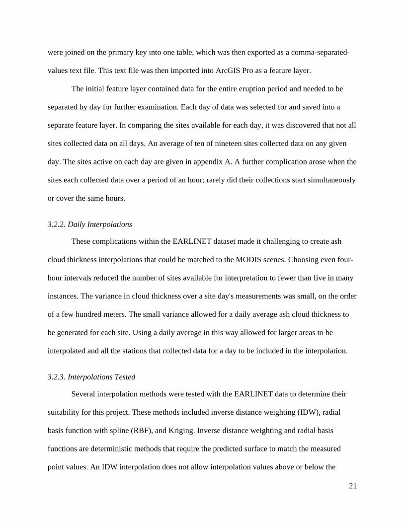
The three interpolations were tested using data from the same date, April 16, at the
beginning of the eruption, which had nine active stations. Both of the IDW and RBF
interpolations required at least three nearest neighbors to be included. The results of these two
interpolations, shown in Figure 6, show a similar spatial distribution of the ash cloud thickness in
the area around Berlin, Germany. Additionally, there are similar, straight-line artifacts near
Poland. The cause of these artifacts is unclear and does not appear on other days during the study
period.
23
An interpolation test with ordinary Kriging was also performed on the mean of the ash
cloud thickness for each site on April 16 2010. This test required at least two nearest neighbors
for the interpolation and used a semivariogram with a stable model. The ArcGIS Pro default
kriging parameters were primarily used for this test for simplicity to provide a basis for
comparison. The results of this test, shown in
Figure 7, differ considerably from the IDW and RBF interpolations. As was previously
mentioned, this project's time constraints made this method a poor choice due to the large
number of variables to consider when using Kriging.
Figure 6. The left image displays the RBF with Spline interpolation, while the right displays
the IDW interpolation.
24
Figure 7. The results of the kriging interpolation.
3.2.4. Inverse Distance Weighting
Inverse distance weighting was chosen as the interpolation method for this project due to
its ease of use and performance. This method takes advantage of the premise that measurements
made near each other are more spatially related than measurements made further apart. As an
exact interpolation, the minima and maxima of the IDW interpolation must occur at measured
points. This results in an interpolation that does not spatially extend past the outermost points in
each direction. Each of the nine study days was interpolated using with IDW using the mean ash
cloud thickness at each station.
25
Inverse distance weighting uses weights inversely proportional to the distance between
the measurement and prediction points (ESRI 2020a). The power factor governs the rate at which
the weights decrease with distance, with higher power factor values decreasing faster than lower
values. A power factor of 2 was used for this study to reflect that ash clouds can change rapidly
with distance.
Another critical aspect of IDW interpolations is the search neighborhood. The search
neighborhood defines how many points must be included in the search and places upper limits on
the number of points to include. Due to the small number of points each day contains, the upper
limit is less important than the number of points to include as nearest neighbors. Each day
processed required at least three nearest neighbors and could include up to fifteen points in a
circular search pattern to consider measurements equally in all directions.
3.2.5. Cross-Validation
Assessing the sensitivity of the Inverse Distance Weighting interpolation of EARLINET
data provide insight into how well the interpolation estimated ash cloud thickness. The
Geostatistical Wizard tool in ArcGIS Pro, through which the IDW interpolation is performed,
generates cross-validation results as a final step for any interpolation available through the tool.
Cross-validation is a method that leaves a random point out of the interpolation,
calculates a predicted value at the point's location, and then compares the prediction to the
measured. An error statistic is generated for each point measurement in this way, and regression
statistics were calculated from these errors (ESRI 2020b).
26
3.3. MODIS Processing Overview
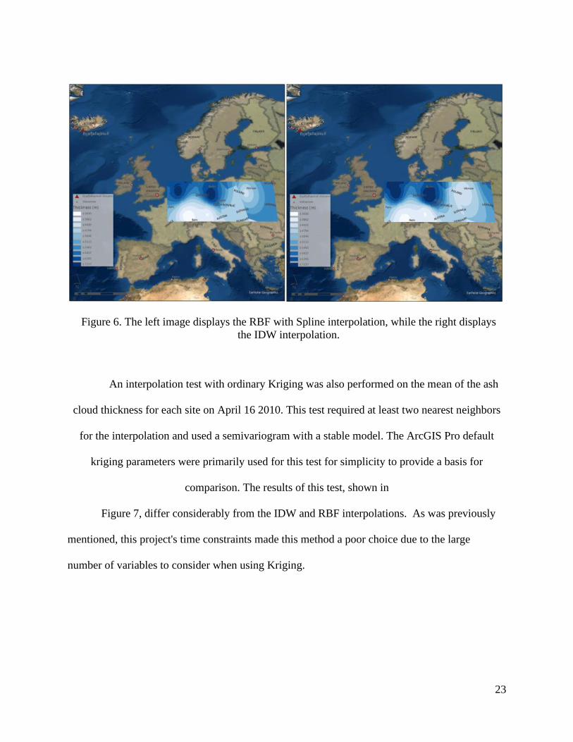
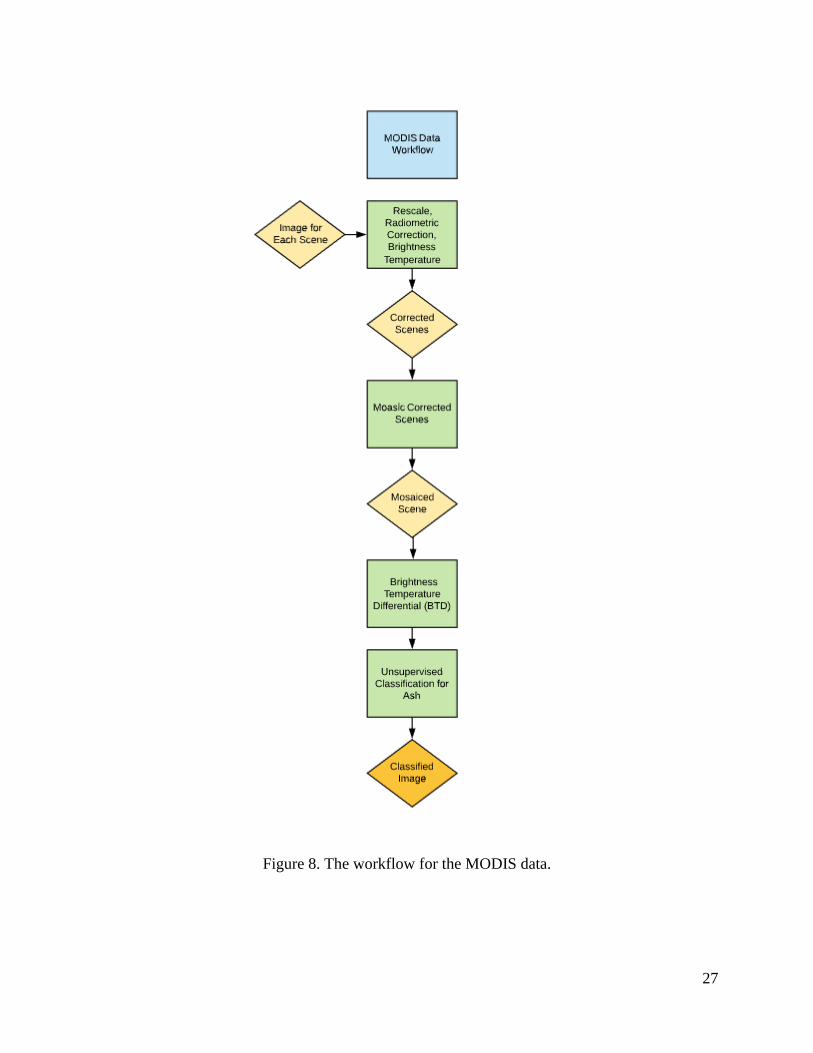
The workflow for MODIS data is shown in Figure 8. This workflow generates a
contoured raster image of the ash cloud densities for three days between April 14 and April 25,
2010. Light yellow boxes in the workflow are input and intermediate data products, dark yellow
represents final products, and green boxes represent data processing steps.
27
Figure 8. The workflow for the MODIS data.
28
3.3.1. MODIS Data Import and Corrections
The study area for the Eyjafjallajökull ash cloud extends from Iceland to Continental
Europe. The TERRA satellite must make several orbital passes to capture multiband scenes of
the entire study area (Oguro, Ito, and Tsuchiya 2011). Differences between scenes obtained on
different orbital passes can result in artifacts when the images are mosaicked, affecting image
classification.
For each of the three days, scenes were downloaded from NASA's LAADS website as
GeoTIFF band files that needed to be imported and converted to a raster format. The GDAL
importation tool in Idrisi was used to import and convert each file into the Idrisi raster format.
Due to variations in satellite altitude, the X and Y resolution values varied slightly
from one raster to another. The Idrisi Project tool was used to set the projections to X = 0.00898
and Y = 0.00901. Unfortunately, there was no bulk processing capability available for this tool,
and each raster needed to be processed manually. Each raster required about five minutes of
processing time. With more than 120 raster files to process, this task required over 10 hours of
processing time. Any future work using this tool for bulk reprojection should involve the model
builder within Idrisi to provide automation support.
3.3.2. Radiance Values
The individual raster files for each day and band have non-physical, digital number (DN)
pixel emissivity values that are not immediately useable for mosaicking or classification. These
DN values must be converted to top of atmosphere (TOA) spectral radiance values prior to
mosaicking. Converting the DN values to the TOA spectral radiance (Lλ) requires the MODIS
rescale gain factor Rscaleλ and the radiance rescaling offset factor Roffsetλ (Oguro, Ito, and
29
Tsuchiya 2011). The relationship between these three values is given by Oguro et al. (2011) in
Equations 1, 2, and 3.
𝐿𝜆 = 𝑅𝑠𝑐𝑎𝑙𝑒 𝜆(𝐷𝑁𝜆 − 𝑅𝑜𝑓𝑓𝑠𝑒𝑡 𝜆) (1)
𝑅𝑠𝑐𝑎𝑙𝑒 𝜆 = 𝐿𝑚𝑎𝑥𝜆 − 𝐿𝑚𝑖𝑛𝜆
32767(2)
𝑅𝑜𝑓𝑓𝑠𝑒𝑡 𝜆 = 32767 − 𝐿𝑚𝑖𝑛𝜆
𝐿𝑚𝑎𝑥𝜆 − 𝐿𝑚𝑖𝑛𝜆 (3)
where Lλ is the pixel spectral radiance in W/(m2‧sr‧µm) for each band, Lminλ and Lmaxλ are
the minimum and maximum band radiances, respectively, in W/(m2‧sr‧µm). While Rscaleλ and
Roffsetλ could be calculated in this way, it is unnecessary to do so as NASA provides these values,
shown in Table 2, for each band acquired in the file metadata. The spectral radiance for each
scene in each band and each day was calculated using the model builder in ArcGIS Pro using
these scale and offset values.
Table 2. Radiance scale and offset values provided by NASA for each of the three bands used in
this project.
Band 29
W/(m2‧sr‧µm)
Band 31
W/(m2‧sr‧µm)
Band 32
W/(m2‧sr‧µm)
Rscaleλ 5.32486942‧10-4 8.40021996‧10-4 7.29697582‧10-4
Roffsetλ 2.73058350‧103 1.57733972‧103 1.65822131‧103
Converting the raster scenes from DN to radiance values is an essential step for
generating correctly mosaiced images. When scenes were mosaiced prior to this step, there were
far more artifacts from the mosaicking process where the scenes overlapped. This step is also
necessary to convert the radiance values into temperature values described further in this chapter.
30
3.3.3. Image Mosaic
Once all the scenes for a day have been corrected and transformed, they need to be
mosaicked into one large image. Mosaicking joins scenes together, aligning the edges using each
scene's geospatial information. The purpose of mosaicking the scenes together into one image is
to reduce the number of raster files being processed, speeding up the processing time, and
decreasing the final raster size.
Generating the final mosaic images requires first creating empty mosaic rasters. These
rasters were created with 32-bit unsigned float values using the Create Raster Dataset tool in
ArcGIS Pro. It is necessary to use the 32-bit unsigned float pixel type because of The conversion
from digital numbers, which are integers, to scaled radiance values, which become floating-point
values when calculated. The newly generated empty rasters were then used as containers for the
mosaic operation.
Each day of data contained a morning and an evening orbital pass, which entirely
overlapped spatially. To preserve any temporal differences that might occur over a day and
prevent issues that may arise from averaging two sets of rasters over the entire study area, a
morning mosaic and an evening mosaic for each band and each day were created. Although this
increases the number of mosaicked rasters to process, it allows for more comparison with the
EARLINET interpolated rasters.
The scenes for each half-day were mosaicked for each of the three bands used in this
project. The Mosaic tool in ArcGIS Pro was used to create the 18 mosaicked images. Where the
scenes overlapped with each other, the mean between each scene was calculated to blend the
scenes and remove noticeable seams. Background values at the edges of scenes were ignored to
remove hard lines that would otherwise create straight-line artifacts in the finished mosaic. Color
31
matching was not performed as any attempts of this resulted in the failure of the mosaic
operation.
3.3.4. Brightness Temperature
Before the mosaicked rasters can be classified, the radiance values must be converted to
brightness temperature values in Kelvin. The conversion from radiance to temperature follows
Plank's law for blackbody radiation (Oguro, Ito, and Tsuchiya 2011). The wavelength form of
the equation for blackbody radiation is given in Equation 4:
𝑇𝑏 =
ℎ𝑐𝑘𝜆
ln(2ℎ𝑐2 (𝐿𝜆𝜆5 × 10⁻⁶) + 1)⁄(4)
where Tb is the brightness temperature in kelvin, h is Plank's constant, c is the speed of light in a
vacuum, k is Boltzmann's constant, λ is the central wavelength of the spectral band, Lλ is the
spectral radiance given in Equation 1.
Calculating the brightness temperature is band dependent, and the numerator does not
change between mosaicked images of the same band. A model for the brightness temperature
conversion was created for each of the three bands and used to produce mosaicked temperature
rasters. These rasters were then used to produce a brightness temperature difference
classification.
3.3.5. Ash Cloud Classification
Calculating the spatial extent of volcanic ash requires detecting the ash cloud in a
remotely sensed scene. Brightness temperature differences (BTD) between two thermal infrared
channels are used to distinguish ash particles from water vapor. Particles of volcanic ash strongly
32
absorb light at a wavelength of 10.8 µm with a lesser absorption at 12 µm; the reverse is true for
water vapor (Emeis et al. 2011). Francis et al. (2012) suggest a three-channel BTD incorporating
the level of erupted SO2, which they developed during the 2010 Eyjafjallajökull eruption. A pixel
would be classified as containing ash if it meets the requirements of Equation 5, where BT is the
brightness temperature of a pixel at the specified wavelength.
𝐵𝑇10.8 − 𝐵𝑇12.0 + 𝐵𝑇10.8 − 𝐵𝑇8.7 < 1.5 𝐾 (5)
This brightness temperature difference calculation, when written in terms of the MODIS
bands, becomes Equation 6.
𝐵𝑇𝑏𝑎𝑛𝑑 31 − 𝐵𝑇𝑏𝑎𝑛𝑑 32 + 𝐵𝑇𝑏𝑎𝑛𝑑 31 − 𝐵𝑇𝑏𝑎𝑛𝑑 29 < 1.5 𝐾 (6)
The brightness temperature differential for each day was calculated using Raster
Calculator within ArcGIS Pro's model builder. Two BTD rasters per day, one for the morning
and one for the evening, were created in this way. These rasters were then classified using a
manual interval with 10 classes in the Symbology tool. A red-yellow color scheme was chosen
for comparison with the results from Francis et al. (2012).
3.4. Flight Path Proximity
A final purpose in identifying high ash density areas is to determine which portions of the
air space are unsafe for aircraft operations. Air routes based on great circles have been
constructed using the XY to Line tool within ArcGIS Pro from each airport's locations
33
connecting to and from airports within the study area. The air routes are then visually compared
to the ash distribution.
34
Chapter 4 Results
This chapter reviews the key results and comparisons between the ground-based lidar
interpolations of ash cloud thickness, the brightness temperature difference method of ash
classification, and the effect on flight paths in the region. The following sections present these
results in the form of maps and spatial comparisons.
4.1. EARLINET Interpolation
An interpolated raster was created for each day between April 16, 2010, and April 24,
2010. An exception to this was the day of April 25, 2010. On that day, there were too few
stations to create the IDW interpolation, and the operation failed. Interpolations were
successfully created for the other nine days of data. The interpolation operation was quick, and
each day required approximately 5 minutes of processing time to complete.
The differences in the area covered from day to day can be quite large due to the nature
of the IDW interpolation itself. The IDW interpolator does not generate interpolation estimates
beyond the spatial extent of the outermost points. The EARLINET database does not provide
enough information on sites that did not provide data on a day to determine if the site was not in
operation or did not record a backscatter value for the ash cloud. While including sites that
recorded 0 m thickness or no ash in order to generate interpolations with the same spatial extents
would have been ideal, the uncertainty of which sites were entirely offline made this impossible.
The daily interpolations show that the spatial distribution of the ash cloud's thickness
varied considerably from day-to-day. Figures 9 through 17 show the daily interpolated
thicknesses. The area between Germany and the United Kingdom shows consistently thick
values greater than 6000 m on most days until April 23, 2010. The station in Berlin, Germany,
35
experienced ash cloud thicknesses on April 17, 2010, and April 21, 2010, while the station in
Warsaw, Poland, consistently reported lower ash cloud thicknesses around 500 m. These values
represent the endpoints of the range of values across the interpolations. While these endpoints
represent the actual measurements made on those days at those sites, it should be noted that these
two sites may be over and under-reporting the cloud base and top altitudes upon which the
thickness is derived. Comparison with the MODIS derived spatial extent of the ash cloud can
elucidate potential systematic errors in the Lidar measurements.
A spatiotemporal trend in the interpolations is that thicker ash clouds were observed at
the beginning of this phase of the eruption, which moved to the south and thinned considerably
as the eruption lost intensity on April 23, 2010. The increase in thickness at the Berlin, Germany,
station on April 21, 2010, indicates the second influx of ash into this area and agrees with the
results found in Augsburg, Germany, by Emeis et al. (Emeis et al. 2011).
The spatial distribution of the thicknesses predicted by the interpolations is also in
agreement with the spatial pattern presented in the WRF-Chem results shown in
36
Figure 3. Although ash cloud thickness is not a direct comparison to the mass concentrations
reported by the WRF-Chem model, they are relatable. Of particular note is the area of Berlin,
Germany, on April 21, 2010, where both large ash cloud thicknesses and mass concentrations are
estimated in both models.
37
Figure 9. IDW interpolation for April 16, 2010.
Figure 10. IDW interpolation for April 17, 2010.
38
Figure 11. IDW interpolation for April 18, 2010.
Figure 12. IDW interpolation for April 19, 2010.
39
Figure 13. IDW interpolation for April 20, 2010.
Figure 14. IDW interpolation for April 21, 2010.
40
Figure 15. IDW interpolation for April 22, 2010.
Figure 16. IDW interpolation for April 23, 2010.
41
Figure 17. IDW interpolation for April 24, 2010.
4.2. MODIS Brightness Temperature Difference
A mosaiced raster was created for each band of the morning and evening on April 17, 21,
and 24, 2010. The brightness temperature difference (BTD) was calculated for each of these days
and classified. Although these values are in Kelvin, it is a misnomer to think of the BTD as units
of temperature as units of Kelvin can not be negative. Values in the BTD rasters below 1.5 K are
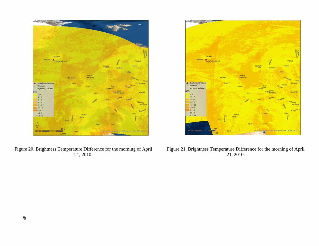
shown in orange and yellow colors in Figure 18– 21, while values above 1.5 K have been made
transparent.
Ash release from Eyjafjallajökull volcano, marked as a red triangle, is clearly seen
immediately south of the volcano in figures 18 and 19. When compared to the MODIS color
composite image from the morning of April 17, 2010, shown in Figure 23, the differences
between water vapor and ash cloud become more apparent. An east-to-west streak of ash north of
42
Scotland becomes apparent, as well as the dispersal of ash into the Scandinavian region of
Northern Europe.
In France and Germany, the middle of Europe appears clear of ash on the morning of
April 17, 2010, by the evening of this day, ash is clearly detected across all of Germany and the
northern regions of France. A significant point of interest is the BTD signal just west of Paris in
Figure 22; when this area is compared with the color composite and the interpolation results for
this day, it becomes clear that ash may be present in higher concentrations than The BTD ash
detection agrees with the interpolation results for this day in this region.
While the BTD in Northern Europe agrees with the interpolation and the color composite
results from NASA, the ash signatures in southern Europe, particularly in Spain and Italy, may
be caused by dust from the Sahara desert in Northern Africa. Unfortunately, there are no
EARLINET measurements recorded on this day for this region, and further analysis is needed to
verify the source of this signal.
The BTD results for April 21, 2010, show that ash has dispersed throughout the study
area. Although there are subtle variations in BTD value, nearly all results are below the 1.5 K
threshold to be classified as ash. The interpolation results for this day show a similar dispersal.
The morning and evening BTD results for April 24, 2010, which are not shown, are
unusual in that all BTD pixel values are less than -50 K. This indicates that either ash was
uniformly dispersed throughout the region in sufficient concentrations to produce a much
brighter thermal image in band 32 or that some issue may exist within the band images
themselves.
The MODIS ash classification results on April 17, 2010, shown again in Figure 24, agree
well with published classifications for this time period. Gudmundsson et al. 2012 published the
43
ash classification using SEVIRI data shown in Figure 25; the results for April 14-17, 2010, are
shown in green. The ash cloud being erupted and blown directly south of the volcano is present
in both classifications. Both classifications also show ash over northern Europe and central
France. The SEVIRI classification also shows ash emanating from the volcano being blown in a
south-easterly direction, which is not apparent in the MODIS classification. This may be due to
the 3 days the SEVIRI classification covers.
44
Figure 18. Brightness Temperature Difference for the morning of April
17, 2010.
Figure 19. Brightness Temperature Difference for the evening of April
17, 2010.
45
Figure 20. Brightness Temperature Difference for the morning of April
21, 2010.
Figure 21. Brightness Temperature Difference for the morning of April
21, 2010.
46
Figure 22. BTD for the morning of April 17, 2020, zoomed in for
comparison purposes.
Figure 23. NASA MODIS color composite for the morning of April
17, 2010.
47
Figure 25. Ash cloud classifications from the SEVIRI
instrument, from Gudmundsson et al. 2012
Figure 24. Brightness Temperature Difference for the
evening of April 17, 2010.
48
4.3. Flight Paths
The European airspace was closed to most air traffic between April 15, 2010, and April
21, 2010 (Ulfarsson and Unger 2011). However, the MODIS BTD analysis shows that some
airspace in southern Europe may have been able to remain open until the afternoon of April 17,
2010, and this is indicated in Figure 26, where thin, light-blue lines indicate flight paths between
international airports. As the conditions were rapidly changing, the airspace would have needed
to be closed as higher ash concentrations moved across central Europe into more southern
regions.
Air travel restrictions were lifted on April 21, 2010. As the BTD results for this day
show, ash was widely dispersed across the entire study area. Even though this would seem to
preclude any flight paths from being open, the BTD method does not provide enough
information on ash concentration to determine if the ash present was below the 200 µg/m3
density limit for most aircraft to operate safely.
49
Figure 26. Air routes across Europe along with the BTD ash signal on the morning of April 17,
2010.
50
Chapter 5 Discussion
This study's objective was to determine how well an interpolation based on a set of sparse
ground-based Lidar stations can estimate the spatial distribution of a volcanic ash cloud in
comparison to the brightness temperature difference computed from MODIS satellite imagery.
This study's additional goal was to provide insight to airline managers and government officials
and help them determine when to institute air route suspensions.
This chapter addresses the implications of this project, along with the challenges and
limitations of the methods used. This research's future is also discussed with an in-depth
discussion of the methods necessary to extend this project.
5.1. Discussion
Determining the extent and attributes of a volcanic ash cloud is vital to the modern world
of avionics and natural disaster risk mitigation. However, it is not an uncomplicated assessment
to make. There are several ways in which ash clouds can be monitored, and the two methods
examined here represent only a subset of observational possibilities.
The results of this study were threefold. First, the EARLINET Lidar data's daily
interpolations present snapshots of the variability in the spatial distribution of ash cloud
thickness. This method generates a regional picture of what might be happening between sparse
measurement points.
A ground-based Lidar network's ability in studying air quality may appeal to
governments with limited funds for the dual use of monitoring environmental quality and natural
disaster hazard mitigation. However, operating a network of this type requires many highly-
skilled and knowledgeable people to maintain the equipment. Additional people and computing
51
resources would be required to process and analyze the backscatter data and then to build the
spatial interpolations.
Next, the brightness temperature difference method allows for a high resolution (1 km)
examination of the ash cloud and its dispersal over several days. This method separates ash
particles' thermal signal from that of water vapor, which allows the spatial distribution of ash to
be determined even when there is significant cloud cover.
Last, the comparison of flight paths with the spatial distribution of ash provides some
insight into when it may be necessary to institute air space restrictions. It is always correct to
make a more prudent judgment when lives are at stake. The BTD analysis results show that the
spatial distribution of ash was limited to Northern Europe until the afternoon of April 17, 2010,
when conditions changed suddenly over Germany and France. While some aircraft may have
been able to fly based on the BTD results, the daily interpolations indicated an earlier extent of
ash into this region.
5.2. Limitations
Both methods presented here have produced useful and insightful results. Neither method
is flawless, and both have issues that require further study. This section examines the challenges
and limitations encountered in this study.
5.2.1. EARLINET Interpolations
The EARLINET data was straightforward to access and use for interpolation. The
relative ease of acquiring the database and generating an interpolated raster of ash cloud
thickness belies the analysis required to produce such a database. The EARLINET project relies
on each Lidar station's managers to process the raw data into backscatter data through their
Single Calculus Chain algorithm. Researchers with the EARLINET project then analyzed these
52
backscatter results to determine the altitude of the ash cloud. While this is convenient for the
end-user, attributes such as particle density and the atmosphere's optical thickness are not
reported.
In this study, the daily mean of the ash cloud thickness was used for the IDW
interpolation. This was done because the number of observations and observation times did not
align between sites. Additionally, not all sites within the network recorded data for the entire
duration of the eruptive event. This makes the EARLINET database more challenging to analyze
and maybe a design consideration for other Lidar networks.
5.2.2. MODIS and BTD
Although the BTD analysis results were striking and insightful compared to the
EARLINET interpolation, this represented the most challenging portion of the project. The
preparation of only three days of data required processing more than 120 scene files over three
bands and two software platforms. This represents a significant computing challenge that may be
better served by the development of custom software to facilitate processing individual scenes
into a mosaic.
The brightness temperature difference was a straightforward process but did not always
produce results that are easily understood. While the BTD process successfully separated the ash
and water vapor signals, there were still areas classified as ash that were water vapor clouds or
even ice, such as over parts of Greenland. It is unclear why this method produced ambiguous
results in certain areas. It is also unclear why this method entirely failed for April 24, 2010. In
this project, the study area was large, which may contribute to the BTD method's ambiguous
results.
53
5.3. Future Research
The results presented here represent a small subset of what is necessary to generate a full
hazard analysis of an eruptive event. While the spatial distribution of an ash cloud is essential to
understanding what areas might be impacted, the ash cloud's density determines the amount of
risk it poses. The next steps in this research would be to calculate the ash cloud thickness and
density and ultimately estimate the volume of erupted material.
5.3.1. Ash Cloud Thickness
While ash cloud thickness was the primary data available from ground-based Lidar, a full
aviation hazard assessment would need observations in areas, such as over the oceans, where it is
impractical to place ground-based Lidar systems. Determining the thickness of the ash cloud is
less straightforward than determining the BTD. Dubuisson et al. (2014) suggest that the
thickness of the ash layer, L, can be obtained for each pixel using Equation 7 for the optical
thickness, τa, as a function of the extinction efficiency, Qext, the particle size distribution, n(r),
and the particle radius, r.
𝜏𝑎(𝜆) = 𝜋𝐿 ∫ 𝑟2
∞
0
𝑄𝑒𝑥𝑡(𝜆, 𝑟)𝑛(𝑟)𝑑𝑟 (7)
Several of the parameters in equation 5 may be estimated as a priori values to provide an
estimate of the ash layer thickness, L, at each pixel. This method would require the MODIS
aerosol optical depth as an additional data product. The thickness could then used to calculate
both the Eruptive Volume and the mass loading in the next two sections.
5.3.2. Eruptive Volume
Once the ash cloud classification is complete and the ash cloud thickness, L, is calculated
for each pixel, it is straightforward to find the volume of each pixel by multiplying the pixel area
54
by the ash layer thickness. The eruptive volume of ash is then the sum of volume for each pixel.
In addition to being useful to a hazard assessment, this measurement is useful to geologists and
for determining the volcanic explosivity index of an eruptive event.
5.3.3. Ash Cloud Density Contours
Ash cloud density is what produces the most risk to people, air quality, and aircraft. The
density of ash particles within the ash cloud can be determined using the equation for mass
loading, M, and the layer thickness, L, for each pixel (Equation 8):
𝑀 = 4
3𝜋𝜌𝑟𝑒
3𝜏𝑎
𝑘𝑒𝐿(8)
where ρ (kg m-3) is the density of the rock from which the ash was created, re is the effective
radius of each particle, and ke the extinction coefficient in meters. As the ash cloud's density is
the mass per unit volume, the density per pixel could be found from the pixel volumes.
5.4. Conclusions
This project achieved its objectives of determining the efficacy of using interpolated
ground-based Lidar for determining the risk caused by explosive volcanic eruptions. These daily
interpolations were compared with high resolution, thermal satellite imagery analysis, and found
to be comparable. The spatial analysis results of the ash cloud distribution were considered in
relation to its effects on air travel and risk mitigation by airline managers.
In the future, the analysis would include automation of the satellite image processing
steps. Future goals would include expanding the project to include estimates of the ash cloud
density, thickness, and eruptive volume. With increasing computing power and automation,
classification methods using freely available MODIS imagery become economical choices for
developing regions. A single, highly trained individual would be capable of generating an ash
55
classification useful in making airspace risk assessments. Ground-based Lidar networks are
capable of producing comparable interpolations of the spatial distribution of an ash cloud.
Without such a network already in place, it is not an economical choice even when processing
satellite imagery challenges are considered.
Explosive volcanic eruptions represent significant risks that must be mitigated by
counties and airline managers around the world, even in locations far from a volcano. This work
may provide some insight and may be useful to natural hazard risk managers in developing
countries.
56
References
Amato, Francesco, Giuseppe D’amico, Lucia Mona, Claudio Dema, and Sergio Ciamprone.
2019. “EARLINET Data File Structure.” https://www.unidata.ucar.edu/software/netcdf/.
BBC News. 2010. "Iceland's Volcanic Ash Halts Flights in Northern Europe." BBC News. 2010.
http://news.bbc.co.uk/2/hi/8622978.stm.
Casadevall, Thomas J. 1994. "The 1989-1990 Eruption of Redoubt Volcano, Alaska: Impacts on
Aircraft Operations." Journal of Volcanology and Geothermal Research 62 (1–4): 301–16.
https://doi.org/10.1016/0377-0273(94)90038-8.
Casadevall, Thomas J, Perla J Delos Reyes, and David J Schneider. 1996. "The 1991 Pinatubo
Eruptions and Their Effects on Aircraft Operations." Fire and Mud: Eruptions and Lahars
of Mount Pinatubo, Philippines, 625–36. https://www.unisdr.org/files/3000_USGS2.pdf.
Christopher, Sundar A., Nan Feng, Aaron Naeger, Ben Johnson, and Franco Marenco. 2012.
"Satellite Remote Sensing Analysis of the 2010 Eyjafjallajökull Volcanic Ash Cloud over
the North Sea during 4-18 May 2010." Journal of Geophysical Research: Atmospheres 117
(D20). https://doi.org/10.1029/2011JD016850.
CIA. 2020. "Europe :: Iceland — The World Factbook - Central Intelligence Agency." The
World Factbook. 2020. https://www.cia.gov/library/publications/the-world-
factbook/geos/ic.html.
Dubuisson, Philippe, Hervé Herbin, Fanny Minvielle, M Compiègne, François Thieuleux,
Fédéric Parol, and Jacques Pelon. 2014. “Remote Sensing of Volcanic Ash Plumes from
Thermal Infrared: A Case Study Analysis from SEVIRI, MODIS and IASI Instruments.”
Atmospheric Measurement Techniques European Geosciences Union 7 (2): 359–71.
https://doi.org/10.5194/amt-7-359-2014ï.
Emeis, S., R. Forkel, W. Junkermann, K. Scḧafer, H. Flentje, S. Gilge, W. Fricke, et al. 2011.
"Measurement and Simulation of the 16/17 April 2010 Eyjafjallajökull Volcanic Ash Layer
Dispersion in the Northern Alpine Region." Atmospheric Chemistry and Physics 11 (6):
2689–2701. https://doi.org/10.5194/acp-11-2689-2011.
ESRI. 2020a. "How Inverse Distance Weighted Interpolation Works—ArcGIS Pro |
Documentation." 2020. https://pro.arcgis.com/en/pro-app/latest/help/analysis/geostatistical-
analyst/how-inverse-distance-weighted-interpolation-works.htm.
———. 2020b. "Performing Cross-Validation and Validation—ArcGIS Pro | Documentation."
2020. https://pro.arcgis.com/en/pro-app/latest/help/analysis/geostatistical-
analyst/performing-cross-validation-and-validation.htm.
Francis, Peter. 1989. "Remote Sensing of Volcanoes." Advances in Space Research 9 (1): 89–92.
https://doi.org/10.1016/0273-1177(89)90471-7.
57
Francis, Peter, Michael Cooke, and Roger Saunders. 2012. "Retrieval of Physical Properties of
Volcanic Ash Using Meteosat: A Case Study from the 2010 Eyjafjallajökull Eruption."
Journal of Geophysical Research: Atmospheres 117 (D20).
https://doi.org/10.1029/2011JD016788.
Francis, Peter, and David Rothery. 2000. "Remote Sensing of Active Volcanoes." Annual Review
of Earth and Planetary Sciences 28 (1): 81–106.
https://doi.org/10.1146/annurev.earth.28.1.81.
Gasteiger, J, S Groß, V Freudenthaler, and M Wiegner. 2011. "Volcanic Ash from Iceland over
Munich: Mass Concentration Retrieved from Ground-Based Remote Sensing
Measurements." Atmos. Chem. Phys 11: 2209–23. https://doi.org/10.5194/acp-11-2209-
2011.
Gudmundsson, Magnús T, Thorvaldur Thordarson, A ´ Rmann Höskuldsson, Gudrún Larsen,
Halldór Björnsson, Fred J Prata, Björn Oddsson, et al. 2012. “Ash Generation and
Distribution from the Eruption of Eyjafjallajökull, Iceland.” Scientific Reports 2 (572): 12.
https://doi.org/10.1038/srep00572.
Hall, Richard, Róbert Erdélyi, Edward Hanna, Julie M. Jones, and Adam A. Scaife. 2015.
"Drivers of North Atlantic Polar Front Jet Stream Variability." International Journal of
Climatology. John Wiley and Sons Ltd. https://doi.org/10.1002/joc.4121.
Horwell, Claire J., and Peter J. Baxter. 2006. "The Respiratory Health Hazards of Volcanic Ash:
A Review for Volcanic Risk Mitigation." Bulletin of Volcanology. Springer.
https://doi.org/10.1007/s00445-006-0052-y.
Jenner, Lynn. 2017. "Terra Spacecraft | NASA." NASA. 2017.
https://www.nasa.gov/mission_pages/terra/spacecraft/index.html.
Langmann, Baerbel, Arnau Folch, Martin Hensch, and Volker Matthias. 2012. "Volcanic Ash
over Europe during the Eruption of Eyjafjallajökull on Iceland, April-May 2010."
Atmospheric Environment 48 (March): 1–8.
https://doi.org/10.1016/j.atmosenv.2011.03.054.
Maccherone, B, and S Frazier. 2014. “MODIS Web.” MODIS Web. NASA. 2014.
http://modis.gsfc.nasa.gov/data/dataprod/.
Madonna, F, F Amato, J Vande Hey, and G Pappalardo. 2015. "Ceilometer Aerosol Profiling
versus Raman Lidar in the Frame of the INTERACT Campaign of ACTRIS." Atmos. Meas.
Tech 8: 2207–23. https://doi.org/10.5194/amt-8-2207-2015.
Massonnet, Didier, and Kurt L. Feigl. 1998. "Radar Interferometry and Its Application to
Changes in the Earth's Surface." Reviews of Geophysics 36 (4): 441–500.
https://doi.org/10.1029/97RG03139.
58
Met Office. 2020. "The London VAAC Process." 2020.
https://www.metoffice.gov.uk/services/transport/aviation/regulated/vaac/process.
NASA. 2020. "The Multispectral Scanner System « Landsat Science." 2020.
https://landsat.gsfc.nasa.gov/the-multispectral-scanner-system/.
Oguro, Yoshinari, Seiji Ito, and Kiyoshi Tsuchiya. 2011. "Comparisons of Brightness
Temperatures of Landsat-7/ETM+ and Terra/MODIS around Hotien Oasis in the
Taklimakan Desert." Applied and Environmental Soil Science 2011: 11.
https://doi.org/10.1155/2011/948135.
Pedersen, Rikke, and F. Sigmundsson. 2004. "InSAR Based Sill Model Links Spatially Offset
Areas of Deformation and Seismicity for the 1994 Unrest Episode at Eyjafjallajökull
Volcano, Iceland." Geophysical Research Letters 31 (14): L14610.
https://doi.org/10.1029/2004GL020368.
Prata, A. J. 1989. "Infrared Radiative Transfer Calculations for Volcanic Ash Clouds."
Geophysical Research Letters 16 (11): 1293–96. https://doi.org/10.1029/GL016i011p01293.
Sigmundsson, Freysteinn, Sigrún Hreinsdóttir, Andrew Hooper, Thóra A ´ Rnadóttir, Rikke
Pedersen, Matthew J Roberts, Níels O ´ Skarsson, et al. 2010. “Intrusion Triggering of the
2010 Eyjafjallajökull Explosive Eruption.” https://doi.org/10.1038/nature09558.
Song, Wenjia, Yan Lavallee, Kai Uwe Hess, Ulrich Kueppers, Corrado Cimarelli, and Donald B.
Dingwell. 2016. "Volcanic Ash Melting under Conditions Relevant to Ash Turbine
Interactions." Nature Communications 7 (1): 1–10. https://doi.org/10.1038/ncomms10795.
Stothers, R B. 1984. "The Great Tambora Eruption in 1815 and Its Aftermath." Science (New
York, N.Y.) 224 (4654): 1191–98. https://doi.org/10.1126/science.224.4654.1191.
Tam, Elizabeth, Rei Miike, Susan Labrenz, A. Jeff Sutton, Tamar Elias, James Davis, Yi Leng
Chen, Kelan Tantisira, Douglas Dockery, and Edward Avol. 2016. "Volcanic Air Pollution
over the Island of Hawai'i: Emissions, Dispersal, and Composition. Association with
Respiratory Symptoms and Lung Function in Hawai'i Island School Children." Environment
International 92–93 (July): 543–52. https://doi.org/10.1016/j.envint.2016.03.025.
Ulfarsson, Gudmundur Freyr, and Elizabeth A. Unger. 2011. "Impacts and Responses of
Icelandic Aviation to the 2010 Eyjafjallajökull Volcanic Eruption." Transportation
Research Record: Journal of the Transportation Research Board 2214 (1): 144–51.
https://doi.org/10.3141/2214-18.
Ward, Peter L. 2009. "Sulfur Dioxide Initiates Global Climate Change in Four Ways." Thin Solid
Films 517 (11): 3188–3203. https://doi.org/10.1016/j.tsf.2009.01.005.
Webley, P. W., T. M. Lopez, A. L. Ekstrand, K. G. Dean, P. Rinkleff, J. Dehn, C. F. Cahill, et al.
2013. "Remote Observations of Eruptive Clouds and Surface Thermal Activity during the
59
2009 Eruption of Redoubt Volcano." Journal of Volcanology and Geothermal Research 259
(June): 185–200. https://doi.org/10.1016/j.jvolgeores.2012.06.023.
Webley, P. W., T. Steensen, M. Stuefer, G. Grell, S. Freitas, and M. Pavolonis. 2012. "Analyzing
the Eyjafjallajökull 2010 Eruption Using Satellite Remote Sensing, Lidar and WRF-Chem
Dispersion and Tracking Model." Journal of Geophysical Research: Atmospheres 117
(D20). https://doi.org/10.1029/2011JD016817.
Wiegner, Matthias, Josef Gasteiger, Silke Groß, Franziska Schnell, Volker Freudenthaler, and
Renate Forkel. 2012. “Characterization of the Eyjafjallajökull Ash-Plume: Potential of
Lidar Remote Sensing.” Physics and Chemistry of the Earth 45–46 (January): 79–86.
https://doi.org/10.1016/j.pce.2011.01.006.
60
Appendix: EARLINET Sites Active By Day
Day Site Hours Operational Number of Observations
April 16, 2010 Belsk 8 4
Cabauw 9.5 10
Hamburg 20 20
Leipzig 20 14
Minsk 4 3
Munich 8.5 6
Neuchatel 16 2
Payerne 19 18
Palaiseau 17 17
April 17, 2010 Belsk 11 7
Cabauw 2 2
Hamburg 24 24
Leipzig 9 7
Minsk 3 3
Munich 22 19
Neuchatel 21 3
Payerne 24 40
Palaiseau 24 24
April 18, 2010 Belsk 16 7
Bucharest 13 5
Cabauw 8 7
Hamburg 24 24
Leipzig 14 18
Munich 22.5 9
Neuchatel 19 3
Payerne 11 20
Palaiseau 24 24
April 19, 2010 Cabauw 1 1
Hamburg 24 24
Ispra 12 12
L'Aquila 2 2
Leipzig 18 21
Minsk 1 1
Munich 23.5 9
Neuchatel 19 6
Palaiseau 16 16
Potenza 0.5 1
61
Day Site Hours Operational Number of Observations
April 20, 2010 Belsk 4 3
Cabauw 4 3
Hamburg 24 7
Ispra 11 11
L'Aquila 6 6
Lecce 9 2
Leipzig 16 15
Minsk 6 2
Munich 22.5 8
Naples 14 11
Palaiseau 15 15
Potenza 2 2
April 21, 2010 Athens 8 7
Belsk 1.5 2
Bucharest 19 10
Cabauw 10 10
Cork 4 4
Hamburg 24 5
Ispra 8 8
L'Aquila 24 9
Lecce 24 13
Leipzig 3.25 4
Minsk 1 1
Munich 24 9
Naples 14 14
Palaiseau 11 11
Potenza 23 24
Thessaloniki 9 9
April 22, 2010 Athens 15 13
Cabauw 4 4
Hamburg
24 23
Ispra 4 3
L'Aquila 3 3
Lecce 12 12
Leipzig 7.5 9
Munich 23.5 21
Naples 16 10
Palaiseau 12 5
Potenza 15 12
Sofia 9 2
Thessaloniki 12 12
62
Day Site Hours Operational Number of Observations
April 23, 2010 Andenes 8 6
Belsk 12 3
Cabauw 10 11
Hamburg 24 23
Mink 1 1
Munich 23.5 21
Palaiseau 24 24
Thessaloniki 6 6
April 24, 2010 Belsk 0.5 1
Cabauw 19 5
Hamburg 17 15
Ispra 2 2
Munich 23.5 21
Palaiseau 8 8
April 25, 2010 Belsk 1 1
Munich 13 4