Clean Water Makes You Dirty: Water Supply and Sanitation Behavior in Metro Cebu, the Philippines ∗ Daniel Bennett † December 10, 2006 Abstract Water supply improvements are a frequent policy response to endemic diarrhea in de- veloping countries. However, these interventions may unintentionally cause community sanitation worsen. Such a response could occur because improved water supplies desen- sitize the community to the consequences of poor sanitation. Since sanitary behaviors have large externalities, the health impact of this endogenous response may overwhelm the direct benefit of clean water. This paper shows how the expansion of municipal piped water in Metro Cebu, the Philippines has exacerbated public defecation, garbage disposal, and diarrhea. I rely on instrumental variables and household fixed effects to rule out non-causal explanations for these results, and find that a neighborhood’s complete adoption of piped water increases the likelihood of observing excrement or garbage by 15-30 percent. Such a change increases diarrhea incidence by at least 3 cases per household per year. Based on these findings, I develop a model in which sani- tation is a privately-provided local public good. Empirical tests support this framework, highlighting the importance of community dynamics for sanitation and health. ∗ Special thanks to Kaivan Munshi for much support and advice. Nate Baum-Snow, Jillian Berk, Pedro Dal B´o, Andrew Foster, Alaka Holla, Robert Jacob, Ashley Lester, Christine Moe, Evelyn Nacario-Castro, Mark Pitt, Olaf Scholze, Svetla Vitanova and Nicholas Wilson provided many helpful suggestions. Thanks to Anton Dignadice, Connie Gultiano, Rebecca Husayan, Jun Ledres, Ronnell Magalso, Edilberto Paradela, Robert Riethmueller, Ed Walag and Slava Zayats for assistance with data and contextual information. † Brown University, Box B, 64 Waterman Street, Providence, RI, 02912, United States; Daniel [email protected]
Transcript
Clean Water Makes You Dirty:
Water Supply and Sanitation Behavior
in Metro Cebu, the Philippines∗
Daniel Bennett†
December 10, 2006
Abstract
Water supply improvements are a frequent policy response to endemic diarrhea in de-veloping countries. However, these interventions may unintentionally cause communitysanitation worsen. Such a response could occur because improved water supplies desen-sitize the community to the consequences of poor sanitation. Since sanitary behaviorshave large externalities, the health impact of this endogenous response may overwhelmthe direct benefit of clean water. This paper shows how the expansion of municipalpiped water in Metro Cebu, the Philippines has exacerbated public defecation, garbagedisposal, and diarrhea. I rely on instrumental variables and household fixed effectsto rule out non-causal explanations for these results, and find that a neighborhood’scomplete adoption of piped water increases the likelihood of observing excrement orgarbage by 15-30 percent. Such a change increases diarrhea incidence by at least 3cases per household per year. Based on these findings, I develop a model in which sani-tation is a privately-provided local public good. Empirical tests support this framework,highlighting the importance of community dynamics for sanitation and health.
∗Special thanks to Kaivan Munshi for much support and advice. Nate Baum-Snow, Jillian Berk, PedroDal Bo, Andrew Foster, Alaka Holla, Robert Jacob, Ashley Lester, Christine Moe, Evelyn Nacario-Castro,Mark Pitt, Olaf Scholze, Svetla Vitanova and Nicholas Wilson provided many helpful suggestions. Thanksto Anton Dignadice, Connie Gultiano, Rebecca Husayan, Jun Ledres, Ronnell Magalso, Edilberto Paradela,Robert Riethmueller, Ed Walag and Slava Zayats for assistance with data and contextual information.
Diarrheal diseases kill millions of people in developing countries each year, more than eithermalaria or tuberculosis (WHO 2002). Inadequate sanitation is the root cause of diarrhea,since infected waste is a critical aspect of the fecal-oral transmission of these diseases.Poorly-contained waste is a direct hazard to anyone coming into contact with it. It alsoseeps through the soil to contaminate local groundwater sources. Because they lack naturalimmunity, children are particularly vulnerable to diarrhea, and most deaths occur amongchildren younger than two.
Common interventions to combat diarrhea include improvements in water supply, la-trine construction, and education campaigns touting the benefits of sanitation and hy-giene. Researchers have studied the relative effectiveness of these interventions (Esrey etal. 1991, Fewtrell et al. 2005), but have payed little attention to the underlying incentivesand behaviors that perpetuate the problem. These studies typically suppose that exogenousinterventions determine water supply and sanitary infrastructure and that the household’sawareness of disease risks is the primary determinant of its behavior. Lacking a notionthat sanitary practices may be endogenous to water supply, policymakers have emphasizedimprovements in drinking water as an anti-diarrheal intervention. A thematic documentfrom the recent 4th World Water Forum (2006, p. 82) opines, “Water supply and sanita-tion . . . are words that often appear together in speeches and pronouncements. Sanitation. . . somehow disappear[s] during the planning, policy-making, budgeting, and implementa-tion phases, while the lion’s share of effort and resources are allocated to water supply.”Such an emphasis on water supply may be counterproductive if communities trade off watersupply investments with less rigorous sanitation.
While the costs of clean behavior are private, the benefits are public. Without gov-ernment provision of waste disposal, households manage their own waste by constructingand maintaining latrines, and by adhering to sanitary protocols. However, the household’sactions impact the entire community. Public defecation increases the risk of transmissionto anyone who might contact the waste, either directly or through the water supply. In thiscontext, social norms are likely to evolve to promote sanitation. These rules of behaviorfurther the provision of a public good by overcoming the short-term incentive to free-rideoff of others’ behavior. A social norm of cleanliness implies some mutual inconvenience, andthe sustainability of this regime depends on how much the community values sanitation.
Piped water may reduce the benefit of sanitation in two ways. With poor sanitation,waste enters the groundwater through the soil, polluting the locally-drawn water supply.In contrast, the quality of piped water is invariant to local pollution because this source
1
is extracted outside the neighborhood. This partially protects the recipient from waste inthe local environment and makes unsanitary conditions less hazardous. Moreover, pipedwater boosts recipients’ health directly because it generally contains less contaminationthan alternative sources. If sanitation and clean water are substitutes as health inputs, arecipient of piped water derives less benefit from incremental sanitation. Through eithermechanism, piped water desensitizes recipients to sanitary conditions, shrinking the benefitthat the recipients derive from the public good. Cleanliness becomes unsustainable asan equilibrium when a critical mass of the community is sufficiently desensitized. Thismechanism may generate the counterintuitive result that piped water actually exacerbatesdiarrheal disease.
This paper examines the effect of piped water on sanitation and health in Metro Cebu,the Philippines. As the government has expanded piped water service in recent decades,sanitary conditions have deteriorated, and areas with the greatest access exhibit the mostsevere contamination and diarrhea incidence. OLS regressions show that these correlationsare strong and statistically significant, but do not establish causality. To find a causal effectof piped water on sanitation and health, I sequentially employ household fixed effects andinstrumental variables, which are subject to divergent sources of bias. These specificationsfind that piped water has a comparable effect, pointing to a causal rather than spuriousrelationship. Depending on the specification, a neighborhood’s complete adoption of pipedwater increases the likelihood of observing excrement or garbage by 15-30 percent. Such achange increases diarrhea incidence by at least 3 cases per household per year.
A model in which sanitation is a local public good explains these findings and offersadditional predictions. Without government provision, households must decide whether toclean up their waste, and thereby contribute to the local sanitary regime. Multiple equilib-ria are possible, with high and low levels of sanitation, depending upon the community’sability to cooperate. Cleanliness is costly, and the household only participates if the benefitsfrom the clean equilibrium outweigh the inconvenience of participating. With greater pipedwater prevalence, fewer households are invested in the clean regime, and the prospect for co-operation declines. In this framework, the particular equilibrium in the community dictateshousehold behavior, and the household’s own water source is irrelevant for its sanitation.Given these dynamics, piped water has two countervailing effects on health. It improves thehealth of its recipients by exposing them to fewer waterborne pathogens. However, pipedwater reduces everyone’s health by exacerbating unsanitary conditions. The technology’soverall health impact depends upon the relative magnitudes of these effects.
Empirical tests support this framework, highlighting the distinction between the house-hold’s own water supply and community-wide prevalence of piped water. Regressions that
2
distinguish between these variables show that prevalence of piped water is an importantdeterminant of household sanitation, but household’s own water source has a precisely-estimated zero effect. In diarrhea regressions, households with piped water have less diar-rhea, but greater prevalence of piped water exacerbates disease. The importance of pipedwater prevalence suggests that the enforcement of community norms is an important deter-minant of sanitation, and hence diarrhea.
2 Motivation
Anti-diarrheal interventions are a frequent target for development assistance, particularlygiven the recent efforts around the Millennium Development Goals. Calling water supplyand sanitation one of the Big Five development interventions, Sachs (2005, p. 236) hasurged the international donor community to think, “round the clock about one question:how can the Big Five interventions be scaled up in [poor rural areas].” (emphasis in original)He urges that “Sooner rather than later, these investments would repay themselves not onlyin lives saved, children educated, and communities preserved, but also in direct commercialreturns.” The desire to take massive action against these problems is noble. However,these investments are unlikely to succeed if policymakers misunderstand how recipientsmay respond to such interventions.
Confusion in the public health literature about the effectiveness of water supply inter-ventions may point to unmeasured behavioral interference with these experiments. Publichealth studies (summarized in Fewtrell et al. 2005) sometimes conclude that water supplyimprovements reduce infant diarrhea, but sometimes find the opposite (Esrey et al. 1988, Ry-der et al. 1985). Other papers show that the health gains of piped water are contingentupon wealth (Jalan and Ravallion 2003) and the existence of sanitary facilities (Esrey 1996).The confusion in the literature is consistent with a behavioral response that interferes withintended effect of the intervention.
Historical evidence supports the idea that sanitary practices are endogenous to theprevailing disease environment. In the late 19th and early 20th centuries, the United Statesdeveloped a strong tradition of cleanliness, which was useful in combating epidemics ofyellow fever and cholera (Hoy 1995, ch. 2-3). However, behaviors changed in mid-century,coincident with the development of penicillin and the first vaccines. Hoy comments, “Yeteven as personal cleanliness was recognized as a quintessentially American value, publicplaces became dirtier [after World War II]. According to Edna Ferber, the well-travelednovelist, New York City was “the most disgustingly filthy” city in the world in the mid-1950s, and litter and rubbish had already begun to turn “ribbons of green countryside
3
along the highways into casual dumps.”” (p. 173) In Hoy’s view, these changes came aboutbecause recent technological advances reduced the role of cleanliness as a major influenceon health. Sanitation requires time and effort, and people conserve on these inputs whenthe payoffs are low.
While previous authors have not (to my knowledge) studied the endogeneity of sani-tation behavior to water supply, other contexts feature a behavioral response that offsetsa technological improvement.1 Gains in automobile fuel efficiency reduce the per-mile costof travel, and drivers compensate by traveling more (Small and Van Dender 2005, Greene,Kahn and Gibson 1999). An inconclusive debate has explored whether automotive safetyimprovements like seat belts and airbags exacerbate reckless driving by reducing the sever-ity of a potential accident (e.g. Cohen and Einav 2003, Keeler 1994, Peterson, Hoffer andMillner 1995). In the communicable disease context, recent advances in antiretroviral (ARV)therapy for HIV/AIDS have changed the risk calculus of high-risk individuals such as gaymen (Andriote 1999, ch. 10; Dunlap 1996). These drugs dramatically reduce viral loadsin the body, cutting the biological risk of transmission while allowing infected people tolead nearly normal lives. An uptick in risky behavior among gay men has followed thisdecline in the perceived riskiness of unprotected sex, according to several studies (Crepaz etal. 2004, Ostrow et al. 2002, Remien et al. 2005). A recent paper by Lakdawalla, Sood andGoldman (2006) uses interstate variation in Medicaid eligibility as an instrument for HIVtreatment and finds that expansions in treatment increase risky behavior and HIV infection.Like improved water supplies, these drugs are a technological advance that reduces the riskof disease transmission but may provoke a behavioral response.
Externalities are crucial in mediating the impact of compensatory behavior. When thebehavior is strictly private, standard models predict that the technological gain will outweighthe compensatory loss. In the example of automotive fuel economy, traveling additionaldistance imposes relatively small externalities (chiefly in terms of traffic congestion) onother motorists. The aforementioned studies calculate the elasticity of fuel consumptionwith respect to fuel efficiency to be around -0.8: the behavioral response only offsets twentypercent of the technology’s direct effect. When the compensatory behavior exhibits large
1The economics literature examining sanitation or other health behaviors in developing countries issparse. Miguel and Kremer’s (2004b) evaluation of a deworming program in Kenya finds significant positiveexternalities from deworming on school attendance. In another paper, Miguel and Kremer (2004a) find thatindividuals whose social networks include many dewormed people are less likely to seek deworming treatmentthemselves, but the authors attribute this finding to social learning rather than treatment externalities.Alberini and coauthors (1996) examine the role of hygiene and water supply in diarrhea outcomes, andfind that piped water significantly decreases hand washing. Treating the creation of municipal water worksas exogenous, Cutler and Miller (2005) find that piped water adoption resulted in major reductions inmortality in US cities, though Melosi (2000, ch. 8-9) documents multiple sewerage and garbage investmentsthat occurred concurrently.
4
externalities, individual responses are compounded within the community, and the aggregateresponse may more than offset the technology’s direct effect. This scenario describes thecase of ARV drugs for HIV, in which the externalities from risky sex are substantial. WhileARV drugs reduce the biological risk of transmission, rates of HIV infection for gay menhave risen in recent years (CDC 2004, Hall et al. 2003). Considering the parallels betweenpiped water and ARV technologies, water supply improvements may also carry unintendedconsequences.
3 Context and Data
Like many cities in developing countries, Metro Cebu is dirty, congested, and poor. Sit-uated on a small island in the Visayas region of the Philippines, Cebu had 1.6 millioninhabitants in the 2000 census. The metro area abuts the eastern coast of the island, andincludes adjoining Mactan Island and other small islands nearby. Though the populationis concentrated in the urban center, Metro Cebu is defined to include outlying areas thatare sparsely populated. The barangay (neighborhood) is the primary political subdivision,and these areas aggregate into municipalities. Metro Cebu encompasses 296 barangays and10 municipalities. A democratically-elected “captain” leads each barangay and receivesmunicipal funds to maintain public areas and provide basic medical care.
The Metro Cebu Water District (MCWD) provides chlorinated piped water to around40 percent of area households. It sources from 110 production wells, which are high-volumedeep wells located mostly in upland areas. The MCWD stores the water at a handful ofreservoirs around the city and charges subscribers the equivalent of $86 for installation, amonthly fee of $2.70 for a 1/2 inch connection, and $0.30 per cubic meter. Fees are graduatedto subsidize poor households, and the MCWD provides communal taps in disadvantagedareas through a “community well” program. In much of Metro Cebu, the water table isjust a few meters below ground, and many households can extract their own water throughboreholes, dugwells, or artesian springs. Water from these sources has no monetary cost,but is generally less convenient and microbiologically inferior to the piped supply (Moe etal. 1991). Strictly speaking, these private wells are illegal, but the government does notenforce the ban because the MCWD lacks the capacity to meet the implied increase indemand. Seawater intrusion renders local groundwater unpotable in areas near the coast,and local residents must seek water from the MCWD or a private vendor.
The Department of Public Services (DPS) handles sanitation in Cebu, focusing exclu-sively on trash collection. With 63 garbage trucks, the agency collects and deposits around500 tons of waste per day in a centralized landfill located 8 kilometers south of the city
5
center. The level of service in a barangay depends upon the ease of access. While the DPScollects around 90 percent of trash overall, it only collects 77 percent in poor and distantbarangays (Sileshi 2001). The municipal governments fund this agency through propertytaxes and license fees, and barangay governments may supplement this service as needed.No centralized agency handles human waste in Metro Cebu, and residents must maintaintheir own toilets or latrines. Rich households are likely to have flush toilets connected toseptic systems, while poor households may share a public latrine, or use a nearby field orstream. The MCWD’s mandate technically includes human waste management, but theagency has neglected this role in favor of piped water provision.
The primary data source for this paper is the Cebu Longitudinal Health and NutritionSurvey (CLHNS), a household panel survey of roughly 3000 families spanning 22 years. Thesurvey focuses on 33 randomly-chosen barangays in Cebu and follows all households whogave birth in the year beginning in June of 1983. Of the 33 barangays, 17 are designatedas “urban,” representing 74 percent of the sample population. The survey includes 12bimonthly interviews in 1983-85 that deal with the nutrition and health of the mother andinfant. Five subsequent follow-up interviews from 1991 to 2005 focus on age-relevant healthissues. Since the survey selects households based on fertility in 1983-84, it oversamplespoor families, who are more fertile. To understand the role of this selection, Adair et al.(1997) compare mothers of CLHNS children to women in the 1980 Philippines census. Theyfind that the survey is not representative of all Filipina women, but does represent ever-married women with at least once child in the early 1980s. Because the survey tracks thesame cohort for two decades, respondents are disproportionately young in early rounds anddisproportionately old in late rounds.
From the baseline survey and five follow-up rounds, I construct separate datasets toanalyze sanitation and diarrhea outcomes. During interviews, surveyors judged on a scaleof 1 to 4 the amount of excrement and the amount of garbage immediately around therespondent’s house.2 I collapse each measure by combining categories 1 with 2 and 3 with4, a simplification that follows naturally from the wording of the categories. Defecationdata are available in all six panel rounds, while garbage data are available in all but thefirst round. Construction of the diarrhea measure is complicated because, while there arepanel data on diarrhea from 1983-85, water supply is fairly constant over this interval.At each of the initial twelve bimonthly interviews, the survey records whether the samplechild, the sample mother, or others in the household experienced diarrhea in the previous
2The categories for the defecation variable are: 1-heavy defecation in area, 2-some defecation in area,3-very little excreta visible, 4-no excreta visible. The categories for the garbage variable are: 1-lots ofuncollected garbage, 2-some uncollected garbage, 3-very little garbage, 4-no garbage visible.
6
week. I prefer the combination of these measures (whether anyone in the household haddiarrhea), though regressions focusing solely on the sample child give similar results. Sincethere is little variation in water supply over this two-year period, I collapse these data intoa cross-section of counts by summing morbidity outcomes across the twelve rounds.
Variables measuring several household characteristics illuminate patterns in the dataand control for observed heterogeneity in subsequent regressions. Households with moreeducation or wealth may exhibit a stronger preference for sanitation relative to other goodsand face less restrictive budget constraints. The household’s education is defined as themaximum individual attainment within the household. The age of the household headis a proxy for wealth, and I construct this measure using the survey’s designation of thehousehold head. Since dogs, pigs, and roosters are common among Cebu households, anindicator for the presence of animals controls for the waste that they produce. Indicatorsfor whether the household has a flush toilet or no toilet measure the household’s access tosanitary facilities. The household’s age and gender composition may matter, since youngchildren are less restrained in creating mess and gender roles may affect the assignment ofchores. Based on the household roster, I calculate the percent of the household that fallswithin four age bins: 4 and under, 5 to 10, 11 to 15, and older than 15, and also the percentthat is male. The family’s home construction is another wealth indicator. According to thesurvey, a respondent’s housing may either be light, using only nipa or similar materials;medium, based on a wood or cement foundation with nipa walls or roof; or strong, with awood or cement foundation and walls, and a galvanized iron roof.
Cross-sectionally, areas with greater availability of piped water have worse sanitationand health outcomes. Figures 1A to 1C plot piped water prevalence against sanitationand diarrhea. These figures show barangay means, which are calculated across all availablesurvey rounds. There is a noisy but distinctly negative relationship between piped water andsanitation, in terms of both “no defecation” and “no garbage.” The plot of diarrhea againstpiped water prevalence shows substantial variability in incidence among barangays withoutpiped water, with values ranging from 0.7 to 2.8 cases per household. However, all barangayswith non-zero piped water prevalence have incidence exceeding 1.6. A decomposition intohigh- and low-prevalence areas shows the pattern of other household characteristics in theseareas. Table 1 shows the mean and standard deviation of piped water, sanitation andrelated household characteristics, and Columns 1 and 2 split the sample by the averageof piped water prevalence (0.31). High-prevalence areas are dirtier, either in terms of “nodefecation” or “no garbage,” even though other characteristics favor increased sanitationand health. On average, households in these areas have two additional years of educationand are 26 percent less likely to keep animals. They have better access to sanitary facilities,
7
are composed of fewer young children, and live in more robust housing.Trends over time illustrate a similar relationship between piped water and sanitation.
Columns 3 and 4 of Table 1 show how water supply, sanitation, and related characteristicschange from the first to the last survey rounds. The proportion of households with pipedwater expands by 18 percentage points from 1983 to 2005, while the proportion of householdswith “no defecation” declines by 8 points.3 Moreover, trends in other variables do notexplain these declines. Education, which is positively correlated with sanitation, increasesby 2.5 years over this interval, while the share of households keeping animals falls by 7points. By 2005, sample households have fewer young children, better housing, and betteraccess to sanitary facilities. Except for the proportion of respondents in strong housing, allof these differences are statistically significant.4
4 Sanitation, Health, and Piped Water Prevalence
In this section, I estimate the effect of barangay-wide piped water prevalence on sanitationand health. Piped water may affect behavior directly by changing the household’s watersupply technology, or indirectly through norms and externalities. The reduced-form effectof prevalence represents the combined influence of these factors. Since potential instrumentsonly vary by barangay, this specification has the advantage that it can be estimated withinstrumental variables. I estimate the following equations:
sijt = α0 + α1wjt + X ′ijtα2 + εijt (1)
dij = β0 + β1wj + X ′ijβ2 + uij (2)
where i indexes the household, j indexes the barangay, and t indexes the survey round. s
and d are sanitation and diarrhea outcomes, respectively. The proportion of householdsthat use MCWD piped water, w, is calculated in sample including the index household.X is a vector of household characteristics to control for observable heterogeneity acrosshouseholds. In the simplest specification, I only control for age and education, which proxyfor household health preferences and budget constraints. Other specifications include a moreelaborate set of characteristics, including the household’s size, age and gender composition,and whether it keeps animals. Like education and age, these are determinants of sanitation
3The “no garbage” outcome does not exist in 1983. From 1991 to 1998, “no garbage” declined from 0.35to 0.15, before rebounding to 0.45 by 2005.
4Attrition is high in the CLHNS, and could potentially drive some of these trends. However, summarystatistics for non-attriters (not reported) reveal the same patterns in water supply, sanitation, and householdcharacteristics. I discuss attrition further in Section 4.2.
8
and health that may be correlated with water supply. I estimate equation (1) using OLS,fixed effects, and instrumental variables. Without time-series data for diarrhea, fixed effectsregressions are not available to estimate equation (2). In all regressions, I cluster thestandard errors within the barangay, allowing for an arbitrary correlation between errorterms for neighboring households, either contemporaneously or over time. Standard errorsare also robust to heteroskedasticity.
Several potential sources of bias confound the OLS estimates of α1 and β1. Cross-sectional heterogeneity in household and neighborhood characteristics is likely to be corre-lated with sanitation, health, and water supply. For example, urban areas are more likelyto receive piped water, and are also more congested, contributing to poor sanitation andhealth. As the city’s population has grown from 1.0 million in 1980 to 1.6 million in 2000,areas with piped water have seen greater increases in population density, which has exacer-bated unsanitary conditions. Diverging secular trends in sanitation and water supply couldalso spuriously indicate a causal effect.5
Reverse causality raises other identification issues, as sanitary conditions may affect theprevalence of piped water. Planners may target water supply improvements to areas withpoor sanitary or health conditions, inducing a spurious correlation. Planners could alsotarget changes in sanitary or health conditions by delivering piped water to areas that aredeteriorating along these dimensions. At the household level, water supply and sanitationare joint decisions, and sanitary or health conditions may affect the water supply decision.A sanitation or health shock could, in principle, either persuade or dissuade a householdfrom adopting piped water. In one natural story, households seek better health by adoptingpiped water in response to a negative shock. However, households could also adopt pipedwater after a positive shock reveals the benefits of avoiding infection.
Measurement error in piped water prevalence introduces additional bias. w is percentof sample households who receive piped water. However, participants in the CLHNS area small share of any barangay’s population, and this sample average only approximatesthe true prevalence of piped water in the barangay. This sampling variation creates clas-sical measurement error in w. In addition, the survey tracks a non-random subset of thebarangay’s population. Respondents, who all gave birth in 1983-84, are disproportionatelyyoung in early survey years and disproportionately old in later years. Insofar as their watersupply choices are not representative of the wider community, w also contains non-classical
5Residential sorting may introduce bias if households locate throughout the city based on their sanitationpreferences. Residential sorting biases in favor of the findings in this section if inherently cleaner householdsavoid areas with piped water. This is unlikely based on the differences between high and low prevalenceareas in Table 1. Residents in high-prevalence areas are better educated, wealthier, and more likely to beclean based on other observable characteristics.
9
measurement error, which exerts an unknown bias.Given these concerns, I approach identification by exploiting two independent sources
of variation. Both cross-sectional and time-series variation identify the effects of watersupply on sanitation in OLS regressions. Regressions with household fixed effects absorball cross-sectional variation that is time constant, estimating the effect of water supplyfrom changes over time in piped water prevalence and sanitation within a household. Thisapproach removes bias due to fixed geographic or other household heterogeneity. However,fixed effects do not address endogeneity due to sanitation shocks or water supply targetingto poor areas. I address these concerns through instrumental variables regressions. Theseregressions, which rely on time-constant instruments, identify the effect of piped water usingan exogenous component of the cross-sectional variation. The instruments, discussed furtherbelow, are based on geological differences between barangays that are arguably uncorrelatedwith sanitation-related unobservables. Results using OLS, fixed effects, and instrumentalvariables are similar, indicating that the bias in these regressions is not severe and that theestimates represent a causal effect.
4.1 OLS and Fixed Effects
OLS regressions, which appear in Table 2, quantify the correlations in Figure 1 betweenwater supply and sanitation and health. Columns 1 and 4 present the most parsimoniousregressions of sanitation (“no defecation” and “no garbage” respectively) on piped waterprevalence, with controls for age and education. Columns 2 and 5 replicate these regressions,but also control for a more expansive set of household characteristics (age and gendercomposition, household size, and animal ownership). In the linear probability framework,the coefficient represents the effect of a barangay’s complete adoption of piped water onthe likelihood of observing the outcome. Parsimonious specifications (Columns 1 and 4)show coefficients on water supply of -0.24 for “no defecation” and -0.15 for “no garbage.” InColumns 2 and 5, additional controls do not change the effect of piped water, even thoughthese controls are jointly significant. An increase in prevalence of one standard deviation(0.33) is associated with a 7 point increase in the likelihood of defecation and a 5 pointincrease in the likelihood of garbage.
On their own, OLS regressions in Table 2 are identified in part from diverging trendsin water supply and sanitation. It is possible to include year or municipality-year controls,and identify the effect piped water off of deviations from these trends. Coefficients donot measurably change in these regressions when year controls are added, and become
10
slightly stronger with the addition of municipality-year controls (results not reported).6
Population density is the most likely sanitation shock that may spuriously generate aneffect of piped water. Population growth, which has been concentrated in urban areas,may reduce sanitation by straining sanitary facilities. Rounds 2-6 of the survey featurea household-specific measure of density: the number of houses within 50 meters of therespondent. Including this variable in the OLS regressions of Table 2 reduces the pipedwater coefficient by 20-30 percent but does not affect its significance.
Regressions that incorporate household fixed effects can control for time-invariant dif-ferences across households. Columns 3 and 6 of Table 2 expand upon prior specifications byincluding household fixed effects. For the “no defecation” outcome, these results are similarto OLS, with a coefficient estimate of -0.22. For “no garbage,” the effect is positive andinsignificant. The lack of “no garbage” data from the first round may explain this result:with less data, the regression loses statistical power, and point estimates may change ifthe effect of water supply is non-uniform over time. To diagnose this problem, I excludethe first round from the “no defecation” fixed effects regressions. Without the first round,regressions for “no defecation” see a similar attenuation and loss of significance under fixedeffects. The coefficient on piped water prevalence is -0.080, with a standard error of 0.083.The large change in the coefficient relative to the standard error suggests that the effectof piped water is stronger in the first round than in later rounds, so that excluding theseobservations weakens the effect. The failure to find an effect in Column 6 notwithstanding,fixed effects results indicate that inherent differences between households do not drive thecorrelation between water supply and sanitation.7
The effect of piped water prevalence on diarrhea appears in Columns 7 and 8 of Table2. The diarrhea outcome, which is only available in the first round of the panel, countsthe number of instances on twelve intervals in which anyone in the household developsdiarrhea. When only age and education are included as controls, the coefficient estimate is0.7, meaning that a standard deviation (0.27) increase in piped water prevalence increasesmorbidity by 0.19 cases per household. Since the survey question inquires about the previous
6Barangay-year controls cannot be used because they are collinear with wjt, which varies by barangay.7Around 40 percent of households move and 40 percent attrit over the 22 years of the CLHNS. To gauge
the impact of relocation and attrition, I reproduce the results of Tables 1-3 (not reported), comparingmovers to non-movers and attriters to non-attriters. Movers are defined as households who ever relocateacross barangays or partition during the survey, and attriters are households who do not report exactlyone observation per round. Movers and non-movers have comparable age and household composition, butnon-movers are 0.35 years better educated, slightly dirtier, and have worse health. Attriters are slightlyyounger and one year less educated than non-attriters. Sanitation estimates are up to 50 percent larger anddiarrhea estimates are double for movers than for non-movers. Estimates for sanitation are 50 percent largerfor attriters while the effect on diarrhea is 40-100 percent larger for non-attriters. However, the results forthese groups are qualitatively similar.
11
week, but two months elapse between survey intervals, scaling this effect up by 4.35 (the ratioof one month to one week) gives the annualized effect on morbidity, which is at least 0.83cases per household.8 Municipality controls, which absorb some geographic heterogeneity,do not change OLS estimates for diarrhea (not reported).
4.2 Instrumental Variables
Unobserved time-varying factors may generate a spurious effect of water supply in OLS andfixed effects regressions. To address these concerns, I estimate specifications (1) and (2)using instrumental variables. Cebu’s geology naturally limits where groundwater may beextracted, and the instruments capture the technical feasibility of obtaining piped wateror alternative sources. “Kharstic” limestone is the main geological formation underlyingthe city. This limestone is a good conductor of groundwater, and is Cebu’s main sourceof drinking water. Near the coast, a layer of alluvial silt and clay, produced by erosionin the mountains, overlays the limestone. In these areas, seawater intrusion threatensto make groundwater unpotable. Further inland, the terrain becomes mountainous, and avolcanic formation displaces the limestone. The volcanic rock conducts groundwater poorly,so extraction is not feasible in the mountains. The following instruments reflect technicalrealities of groundwater extraction. The first two represent the ability of the municipalagency to deliver piped water to an area, while the last instrument measures the feasibilityof extracting water privately and forgoing piped water service.
• Distance to the Limestone-Alluvial Boundary: The MCWD has exploited the geo-logical boundary between alluvium and limestone for extraction, since this area isinsulated from both saline intrusion and the volcanic zone. Figure 2 is a map of Cebuthat shows the main geological formations in the area and plots the locations of theMCWD’s 110 production wells. These wells are nearly all located along the bound-ary between the alluvial and limestone formations. Transporting water over land iscostly, so barangays far from extraction zones are less likely to receive piped water,all else equal. To capture this variation in the cost of water delivery, I calculate theminimum distance from each sample barangay to the limestone-alluvial boundary asa proxy for the distance to an MCWD production well. Households that are close tothis geological feature are more ready recipients of MCWD piped water, which theagency must only transport a short distance.9
8On each interval, the diarrhea outcome measures whether anyone in the household becomes sick in theprevious week. To the extent that household members develop diarrhea at the same time, this measureundercounts the disease incidence.
9I construct this measure by averaging the distance to the boundary over the area of the barangay. Itis possible to weight the average by population density, based on the location of roads within the barangay.
12
• 40-Meter Elevation Threshold: The limestone-alluvial boundary lies at approximately40 meters above sea level, as do most MCWD wells. Upon extraction, it is mucheasier to transport water downhill, working with gravity, while moving water uphillis technically challenging and costly. Therefore, barangays located above nearby ex-traction points are less likely to receive MCWD piped water. Since the elevation ofmost wells is 35-40 meters, this instrument is an indicator for whether the barangay islocated above 40 meters, on average. Figure 3 shows how this threshold divides MetroCebu and shows the locations of the sample barangays. Most of the populated areaslie below this threshold, however a handful of barangays are uphill from extractionzones, making it much harder to serve these areas.10
• Groundwater Salinity: In areas near the coast, seawater infiltrates the aquifer, mak-ing locally-drawn groundwater unpotable. Residents must seek water from either theMCWD or a private vendor, and the MCWD has met this demand in many commu-nities, even though these areas are relatively far from its source wells. On on a mapof Cebu, Figure 4 shows the salinity gradient for groundwater extracted at the watertable in 1985. This estimate is based on MCWD maps of the 50 parts per million(ppm) contour line. I derive the gradient in Figure 4 by additionally assuming thatthe salinity is 300 ppm (the salinity of brackish water) at the coast, and that thesalinity reaches its natural level at three times the distance inland that is required toreach the 50 ppm contour line (Bowen 1986, Ch. 10).11 The figure shows that sev-eral sample barangays near the coast or on adjacent Mactan Island have groundwatersalinity in excess of 200 ppm, a noticeably salty level. For barangays further inland,salinity levels are less than 50 ppm and private wells are a viable alternative watersource. To limit the influence of urban development on this instrument, I use only1985 values of salinity. Since the 1980s, excessive extraction has played a larger rolein Cebu’s saline intrusion problem, but estimates from 1985 reflect natural salinity to
However, the correlation between the weighted and unweighted measures is around 0.99, so this alternativeadds little value.
10The 40 meter elevation threshold may incidentally capture intrinsic differences between rural and urbanpopulations. As a robustness check, I control for the barangay’s elevation, relying only on the discontinuityat 40 meters to identify water supply variation. With this additional control, the 40 meter threshold remainssignificant in the first stage (t statistic: 3.85), while 2nd stage estimates are smaller but comparable to thebenchmark IV regressions.
11These assumptions, while necessarily arbitrary, are unrestrictive. If anything, salinity at the coastexceeds 300 ppm, however any excess salinity does not incrementally reduce the water’s potability. Sincethe difference between 50 ppm and the natural level of 35 ppm is small, the assumed distance at which theaquifer is unintruded has an insignificant effect on the salinity map. Under these assumptions, Figure 4 fitsapproximately with anecdotal notions of the location of the 250 ppm contour line, which the MCWD alsotracks.
13
a greater degree.12
First stage results based on these instruments appear in Table 3. Each additionalkilometer between a barangay and the boundary reduces prevalence by 2 to 4 percentagepoints, an effect that is significant at 5 percent in the sanitation sample and at 10 percentin the diarrhea sample. Elevation has a strong effect on the availability of piped water: theprevalence is 17 to 27 percent lower (depending upon the sample) in high elevation areas.As expected, areas with higher salinity have greater piped water prevalence, conditional onthe other instruments. An increase in salinity of one standard deviation (65 ppm) increasesthe prevalence of piped water by 13 percentage points in the sanitation sample, and by 5points in the diarrhea sample, although the latter effect is insignificant. The instrumentsare jointly significant in predicting piped water prevalence, but perform better in the largersanitation panel than in the diarrhea cross-section. For sanitation, the F statistic on theinstruments is between 8 and 9, showing strong predictive power. The instruments areweaker in the diarrhea sample, with an F statistic close to 4.
Second-stage estimates based on these instruments appear in Table 4. For sanitationregressions in Columns 1-4, piped water prevalence has a negative and significant effectthat matches the magnitude of OLS and fixed effects estimates. The coefficient ranges from-0.26 to -0.29, depending on the specification, meaning that an increase in prevalence ofone standard deviation (0.34) increases the likelihood of observing defecation or garbage by9 percentage points. These regression perform similarly in specifications that include yeareffects to control for generalized time trends (results not reported).
Results for diarrhea appear in Columns 5 and 6, and the coefficient on piped waterranges from 1.6 to 1.7. Weak instruments may explain why the effect is over twice thesize of the OLS estimate. Although a comparison of the coefficient and standard errorindicates statistical significance, the bias due to weak instruments in both statistics makesthis inference questionable (Dufour 2003). The Anderson-Rubin statistic is an indicator ofthe significance of w that is robust to the bias introduced by weak instruments (Andersonand Rubin 1949). Although this technique does not render a coefficient or standard error,the effect of piped water on diarrhea is non-zero at under 5 percent significance.
While the instruments plausibly exploit exogenous variation in the availability of pipedwater and alternative sources, they may also capture unwanted variation in sanitation.For instance, areas near the city center have high salinity and low elevation, leading the
12Excessive groundwater extraction may exacerbate saline intrusion, but only high-volume extractors suchas breweries or the MCWD are large enough to influence salinity directly. These operations, which typicallydraw water a few kilometers inland, primarily affect the salinity down-gradient in areas near the coast. Abarangay’s water consumption from private wells does not significantly affect the underlying salinity, so itis unlikely that salinity influences sanitation behavior directly.
14
instruments to predict high piped water prevalence. If these areas are also inherently dirtierfor unrelated reasons, IV regressions will spuriously attribute this effect to the water supply.With more instruments than endogenous variables, tests of overidentifying restrictions canevaluate whether the instruments are correlated with the second-stage error term. Table4 reports the Hansen J statistic from a joint test of overidentifying restrictions. With pvalues greater than 0.6 in every case, the tests fail to reject the null hypothesis that theinstruments are exogenous.13
For a second check, I compare the effect of piped water in IV regressions that excludeand include controls for household characteristics. The identifying assumption under IV isthat predicted water supply is uncorrelated with sanitation-related unobservables such aspreferences for sanitation and location-specific sanitary infrastructure. These unobservablesare likely to be correlated with observable household characteristics. If the effect of pipedwater is insensitive to the inclusion of observable household characteristics, it is unlikely tohinge upon the correlation with other unobservables. By this standard, IV results performwell. Comparing specifications with and without these controls in Table 4, coefficientsfor piped water vary by only around 7 percent, despite the joint significance of householdcharacteristics in these regressions.
If the effect of piped water on sanitation is causal, regressions of unrelated outcomeson water supply should not show a negative relationship. As a final falsification exercise, Iinvestigate the effect of piped water prevalence on two measures of educational attainment:school enrollment and grade for age. Both education and sanitation are forms of humancapital investment, and households that value sanitation and health are also likely to valueeducation. Yet schooling is an appropriate variable for falsification tests because a standardmodel does not predict a first-order effect of piped water prevalence on this outcome. Anegative relationship between schooling and piped water prevalence suggests that the effectof water supply on sanitation is spurious; conversely, a finding of no effect on schooling isconsistent with the framework in this paper.
Enrollment and grade for age are proxies for whether the household’s children are cur-rently attending school. School enrollment, which is available in rounds 3-6, is an indicatorof whether each child in the household roster is enrolled in school. Grade for age is a noisiermeasure of school attendance, but is available in round 1, in addition to rounds 3-6. To con-
13I sequentially exclude one instrument from the first stage to check the sensitivity of the IV results tothe instrument set. Exclusion of the elevation threshold instrument depresses the coefficient in sanitationregressions by around 15 percent (not affecting significance) while exclusion of either other instrumenthas a negligible effect. Tests of overidentifying restrictions and first-stage f tests are comparable to before.Omitting the elevation threshold instrument reduces the effect on diarrhea to around 1.0 (losing significance)while omission of either other instrument increases the coefficient to around 2.0.
15
struct grade for age, I divide the child’s grade attainment by his or her age. Since childrenbegin formal schooling at age 6, I normalize age by subtracting 5 from the denominator. Achild who begins schooling at age 6 and remains enrolled will report a grade for age of 1 inevery year, but children who start late or drop out have lower values. For each household,I construct the average of both variables across all school-aged children (ages 6 to 16).
Regressions of enrollment and grade for age on water supply generally find no effect,as illustrated in Table 5. The table displays OLS, fixed effects, and IV results in which thespecifications are consistent with earlier regressions. For enrollment in Columns 1 through3, OLS and IV estimates are between -0.05 and -0.02 and are statistically insignificant. Ac-cording to these estimates, an increase in water supply of one standard deviation reduces thepercent of a household’s children who are enrolled by less than two points. The fixed effectestimate in Column 2 is large, imprecisely estimated, and has the opposite sign of the OLSand IV estimates. With grade for age, regressions in Columns 4-6 find a small but positiveeffect of water supply. This effect is nearly zero in most specifications, but is statisticallysignificant under household fixed effects. Even a significant positive effect on education, iftaken at face value, is inconsistent with earlier findings that piped water worsens sanitation.Other household characteristics behave as expected in these regressions, and both outcomesare increasing in the household’s education, but are decreasing in household size. Overall,I find almost no effect of water supply on these educational outcomes, suggesting that theeffects of water supply on sanitation are not a spurious artifact of the data.14
5 Sanitation as a Local Public Good
Results in the previous section indicate that greater piped water prevalence reduces sanita-tion and health. This section shows formally how these results may arise when sanitationhas large positive externalities. For ease of exposition, I explore the limiting case of positiveexternalities by approaching sanitation as a local public good. This model generates severaltestable predictions that distinguish between the household’s own water source and pipedwater prevalence. I also extend the model to incorporate soil thickness, which similarlydesensitizes the community to unsanitary conditions.
14By construction, regression samples for these outcomes only include households with school-aged chil-dren. This requirement creates attrition in later years of the panel, when respondents’ children are olderthan 16. To ensure that the changes in sample composition do not drive the findings in Table 5, I repeatthe regressions of Tables 2-4 using only the observations for which these educational variables are present.In these regressions, OLS and IV estimates are qualitatively similar, while fixed effects results are similar inthe grade for age sample, but are insignificant in the enrollment sample.
16
5.1 Model Setup
Households, indexed by i, reside in communities of population n and make discrete sanita-tion choices, sit ∈ {0, 1} in each period t. While the t subscripts convey the game’s infiniterepetition, the model is static, and time-constant parameters determine the community’soutcome. Sanitation choices aggregate into community-wide sanitation, st = 1
n
∑sit ∈
[0, 1], and households incur a private cost c when sit = 1, reflecting the expenditure oftime and effort.15 I introduce heterogeneity through γw
i ≥ 0, the household’s sensitivityto dirtiness, and φw ≥ 0, a health endowment. Both parameters depend upon the house-hold’s water source, w ∈ {p, a}, which is either “piped” or “alternative.” The household’ssanitation choice determines its one-shot payoff:
u(sit = 1) = γwi (st − 1) + φw − c (3)
u(sit = 0) = γwi (st − 1) + φw
In this specification, utility can be decomposed into “health,” hwit = γw
i (st − 1) + φw, and“inconvenience,” c. Sanitation is a public good because only st is a health input, whilesit is not. Assuming that γw
i /n < c, expression (3) shows how the household only doesworse by being clean itself. This incentive to free ride leads to a unique Nash equilibriumof non-provision (st = 0) in the one-shot game.
With infinite repetition of the game, the community can enforce a cooperative equilib-rium by threatening to punish households who exhibit poor sanitation. Now, householdsmust weigh the streams of payoffs from “cooperating” (sit = 1) and “defecting” (sit = 0),given the community’s punishment regime. For analytical tractability, I assume that play-ers follow “grim strategies,” punishing a defection by jointly defecting in the subsequentperiod and in perpetuity thereafter.16 With discount rate δ and given previous cooperation,
15Differences in c by water source bear some consideration. In the most likely scenario, cp < ca, sincea ready source of water is necessary to flush a toilet and clean up. This gap, if sufficiently large, couldoverride the decreased sensitivity of piped households, so that increasing prevalence improves sanitation.Since heterogeneity of this nature weighs against the model’s findings, the empirical results suggest thatdifferences in c are minimal.
16The model’s conclusions are equivalent under tit-for-tat strategies, where players punish a defection byjointly defecting for one round. Under this regime, the threshold is γw
i > c(2n + 2δ)/(1 + δ + n), which isgreater than c as long as n > 1. Tit-for-tat has the theoretical infelicity that equilibria other that st = 0and st = 1 may also be subgame perfect, interfering with the computations in (6), (9), and (10).
17
players face the following discounted payoff streams:
u(sit = 1) = φw 1 + δ
δ− c
1 + δ
δ(4)
u(sit = 0) = φw 1 + δ
δ− γw
i
n + δ
nδ
In this expression, u(sit = 1) is the discounted utility the household receives from cooperat-ing from period t to ∞. u(sit = 0) is the discounted utility the household earns by defectingin period t and receiving the punishment of s = 0 from period t + 1 to ∞. Householdsmaximize utility by cooperating if and only if γw
i > c(n + δn)/(n + δ) ≡ τ . Since grimstrategies imply unanimous and perpetual punishment for any defection, complete cooper-ation (st = 1) and non-cooperation (st = 0) are the only subgame perfect Nash equilibria.Households choose their sanitation in unison.17
A straightforward generalization allows for non-unanimous sanitation behavior. Sup-pose the community detects and punishes a defector with exogenous probability, α ∈ (0, 1).Now a household only cooperates if γw
i > c(nδ + nα)/(δ + nα), which equals the originalthreshold when α = 1. For sufficiently low values of α, a subset of the community cancheat on the cooperative equilibrium without being detected, thereby preserving the coop-erative equilibrium. Another way to allow non-unanimous sanitation behavior is to supposethat some players do not participate in the game. If the community recognizes that cer-tain households are always dirty, remaining households may still pursue cooperation amongthemselves. The game proceeds as before among this subset of households, who still makeunanimous sanitation choices.
Cooperation can break down even if everyone prefers the clean equilibrium. Wheneverγw
i > c, the household receives a higher one-shot payoff from the joint cooperation than fromjoint defection. However, households only cooperate when γw
i > c(n+ δn)/(n+ δ), which isgreater than c as long as n > 1. For values of γw
i that are between c and c(n+δn)/(n+δ), thehousehold chooses to defect even though it prefers the one-shot payoff from the cooperativeregime. Intuitively, households in this position choose to free-ride off of others’ contributions
17Perfect complementarity between si and s in health production delivers the same predictions for san-itation and health as the Prisoner’s Dilemma. Suppose s = min(s1, ..., sn), following the familiar Leontifproduction function. Households play a one-shot game with equilibria of either s = 0 or s = 1, and anyindividual can destroy the cooperative equilibrium by not contributing (Cornes and Sandler 1996, pp. 185-190). A household opts out of the cooperative equilibrium if the costs of this regime exceed the benefits,and the health production technology assures that sanitation decisions are unanimous in equilibrium. Thenonnecessity of a repeated game apparatus makes this framework attractive. However, the assumption thatsanitary inputs are perfect complements is unrealistic, since households within the same community are ex-posed to disparate sources of pollution. This model is also less theoretically satisfying because it implicitlyrequires at least one household to prefer the dirty equilibrium for sanitation to decline.
18
to st, creating a wedge between the desirability and sustainability of the cooperative regime.
5.2 The Impact of Piped Water
Piped water conveys a direct health benefit through exposure to fewer pathogens, but alsodesensitizes the household to unsanitary conditions. To formalize these ideas, let φp >
φa, so that piped households have a larger health endowment than non-piped households.Furthermore, define the cumulative distribution function of γw
i , Fw(γ), and let F p(γ) ≥F a(γ). By this assumption, γa first order stochastically dominates (FOSD) γp, meaningthat households have heterogeneous sensitivities to dirtiness, but those with piped watertend to be less sensitive.
For cooperation to be sustainable, every household must be above the threshold. Theprobability that a community obtains the good equilibrium is the product of the individualprobabilities that γw
i is greater than τ : pr(st = 1) =∏
i (1 − Fw(τ)). The prevalenceof piped water matters critically, since piped households are more likely to defect. Whenproportion q of the community has piped water, the probability of cooperation is given by:
pr(st = 1) = (1 − F p(τ))nq(1 − F a(τ))n(1−q) (5)
Differentiating this expression with respect to q shows that the probability of a cooperativeequilibrium declines as more households adopt piped water. The sign of this derivativefollows from the FOSD assumption.
∂pr(st = 1)∂q
=pr(st = 1) × n
(ln(1− F p(τ))− ln(1− F a(τ))
)≤ 0 (6)
Since sanitation behavior is unanimous within the community, the household’s own watersource is irrelevant for its sanitation. The assumption of certain and unanimous punishmentand the exclusion of si from the health production function jointly deliver this prediction.When the model is relaxed to allow for some cheating on the otherwise-cooperative equi-librium, piped households become more likely to cheat than non-piped households.18 Intu-itively, the household’s own water source does not affect its sanitation to the extent thatthe community’s equilibrium in sanitation dictates household behavior. By allowing somehouseholds to cheat, this extension reduces the community’s role in household sanitation.
18Adapting the model to include a non-unitary probability of defection, α, creates a role for a household’sown water supply to affect its sanitation. Here, a household cooperates when γw
i > c(nδ + nα)/(δ + nα),but defections do not necessarily lead to the bad equilibrium. To the extent that piped households are morelikely to defect but these defections go unnoticed, households piped households will tend to be dirtier thannon-piped households.
19
In contrast to this setup, the household’s own water source, rather than piped waterprevalence, influences behavior in a model without sanitation externalities. To illustrate,suppose the household’s health only depends on its own water supply and sanitation: hi =h(wi, si). A household with income yi maximizes utility over health and all other goods (gi),facing the budget constraint that psi + gi = yi. By definition, sanitation is a purely privategood under this scenario. Implicitly differentiating the household’s first order conditionshows the equilibrium relationship between water supply and sanitation:
∂si
∂wi= −∂2h(si, wi)
∂si∂wi/∂2h(si, wi)
∂s2i
< 0 (7)
This derivative is negative if sanitation and clean water are substitutes and health is concavein sanitation. Piped water prevalence does not affect household sanitation in this framework,as it might if either w or s entered the household’s objective function.19
When sanitation is a public good, piped water can easily undermine health by causinga good equilibrium to collapse. This sanitation decline counteracts the benefit that pipedhouseholds receive from cleaner water. To model these effects, define health as the sum ofthe utility derived from sanitation and the endowment : hw
it = γwi (st − 1) + φw, which is
equivalent to overall utility except for inconvenience, c. The sanitation term disappears inthe clean equilibrium, and health equals the endowment, φw. However, households withlarge values of γw
i suffer differentially as sanitation deteriorates.Since the model generates effects of water supply on sanitation that are probabilistic,
the expectation of health across the possible equilibria incorporates the health effects ofa sanitation change. The assumption that players follow grim strategies streamlines theanalysis since only two subgame perfect Nash equilibria exist: st = 0 and st = 1. Takingthe expectation of health across these two outcomes gives the following simplified expression:
E(hwit) = φw − pr(st = 0)γw
i (8)
Piped households have better expected health for two reasons. These households havelarger health endowments, reflecting the greater purity of the piped water supply. Pipedhouseholds also suffer less in the event of a bad equilibrium because they are relativelyinsensitive to the dirty environment. Differencing expected health by water source shows
19w may affect si if piped water prevalence enters the utility or health function directly, but this an implau-sible assumption. Instead, complementarity between si and s can deliver this relationship, either throughthe health or utility function. The public good model presented here is an example of complementarity inutility: si and s are strategic complements since the payoff to taking action sit = 1 is highest when othersare also taking this action (Bulow et al. 1985).
20
this inequality explicitly.
E(hpit − ha
it) = (φp − φa) + pr(st = 0) × E(γai − γp
i ) > 0 (9)
Conditional upon the household’s own water source, greater piped water prevalencecauses the household’s health to worsen by undermining sanitation. The derivative ofexpression (8) with respect to q isolates the “sanitation effect” of greater prevalence.
∂E(hwit)
∂q=
∂pr(st = 1)∂q
× γwi ≤ 0 (10)
The household’s sensitivity, γwi , appears in this derivative, implying a differentially severe
consequence of piped water prevalence for non-piped households, for whom γwi is larger.
Expressions (9) and (10) highlight the countervailing health effects of the piped watertechnology. If the sanitation effect overwhelms piped water’s direct benefit, water supplyimprovements will exacerbate diarrheal disease.
5.3 Soil Thickness: Another Dimension of Sensitivity
The model’s underlying premise is that the community’s exposure to local pollution deter-mines its support for the sanitation regime. For families that drink from local groundwater,the soil is a natural shield against unsanitary conditions. Within the soil, predatory organ-isms and sunlight and moisture fluctuations create a hostile environment that effectivelyfilters out pathogens (Pedley et al. 2004). The soil’s “thickness”–the distance from thesurface to underlying bedrock–affects its ability to attenuate pollution. Thick soil naturallyprotects underlying groundwater from contamination, insulating the community from am-bient pollution in the same manner as piped water. Therefore soil thickness may also affectthe community’s willingness to pursue sanitation.
The direct benefits of thick soil only extend to non-piped households, whose watersupply is subject to contamination through the ground. Since it reduces the contaminationin the groundwater, thick soil increases the health endowment of non-piped households. Italso desensitizes these households by making their water quality less dependent on the levelof surface pollution. To incorporate these features into the model, let the sensitivity andendowments of non-piped households, φa and γa
i , depend on soil thickness, ρ, and assumethat ∂φa/∂ρ > 0 and that ∂γa
i /∂ρ < 0. Soil thickness does not affect the endowments orsensitivity of piped households, so that φw and γw
i do not depend on ρ.This extension leaves intact the essential structure of the model. Households make
dichotomous sanitation decisions, facing an infinitely repeated Prisoner’s Dilemma, and
21
choose to cooperate if and only if γwi (ρ) > c(n + δn)/(n + δ) ≡ τ . Now the soil thickness,
along with the household’s water source, determines whether the household is above orbelow the threshold, τ . Since γa
i is decreasing in ρ, the CDF of γai is increasing in ρ:
∂F a(γ, ρ)/∂ρ > 0. To reach the good equilibrium, every household in the communitymust be above the threshold, so the likelihood of the good equilibrium is the product ofthe individual probabilities that γw
i (ρ) > τ . This expression matches (5), except for themodification making F a a function of ρ. Differentiating with respect to ρ shows that theprospect for a clean equilibrium falls with greater soil thickness.
∂pr(st = 1)∂ρ
= −pr(st = 1)× n(1 − q)1 − F a(τ, ρ)
× ∂F a(τ, ρ)∂ρ
< 0 (11)
Non-piped households, who are less sensitive to their environment with thick soil, drive thisdecline in sanitation. By desensitizing a subset of the community, thick soil functions likepiped water in undermining the cooperative equilibrium.
Soil thickness also mirrors piped water in its effects on health. Thick soil providesa direct health benefit to non-piped households by insulating the local groundwater frompollution. By exacerbating unsanitary conditions, thick soil also worsens health acrossthe community. While non-piped households are subject to both effects, piped householdsonly experience the negative “sanitation effect.” To generate these prediction formally, Imodify the expression for expected health (8) to incorporate the role of soil thickness. Thisexpression is unchanged for piped households, who only experience ρ through the likelihoodof the clean equilibrium. For non-piped households, ρ also enters through the endowment,φa, and the sensitivity parameter, γa
i : E(hait) = φa(ρ) − pr(st = 0)γa
i (ρ). The derivativeof expected health with respect to ρ shows the impact of soil thickness on health for eachgroup.
∂E(hpit)
∂ρ=
∂pr(st = 1)∂ρ
× γpi︸ ︷︷ ︸
−
< 0 (12)
∂E(hait)
∂ρ=
∂pr(st = 1)∂ρ
× γai︸ ︷︷ ︸
−
+∂φa
∂ρ− pr(st = 0)× ∂γa
i
∂ρ︸ ︷︷ ︸+
≷ 0 (13)
For piped households, equation (12) shows that thick soil is unambiguously harmful. Thicksoil reduces sanitation in the community, worsening health among these households. Equa-tion (13) shows the health effect for non-piped households. The first term is the negativeeffect of soil thickness on health through diminished sanitation. The second and third terms
22
capture the direct benefits of thick soil through larger health endowments and reduced sen-sitivity to pollution. Since these benefits counteract the losses from poor sanitation, theoverall effect of soil thickness for non-piped households cannot be signed. If these effectshave similar magnitudes, the net effect is approximately zero.
6 Empirical Tests
By incorporating a strategic framework, the model creates a role for community dynamicsin household sanitation behavior. The sustainability of a cooperative equilibrium dependson the community’s sensitivity to dirtiness, and the particular equilibrium is the primarydeterminant of household sanitation. By desensitizing the community, piped water under-mines the clean equilibrium and causes communities to become dirtier. The technology mayparadoxically exacerbate diarrheal disease if this “sanitation effect” overwhelms the healthbenefit of a cleaner water supply. By extension, soil thickness also insulates and desensitizesthe community, similarly influencing sanitation and health.
6.1 Effects of Piped Water
Previous regressions in Section 4 show that greater piped water prevalence reduces sanita-tion and exacerbates diarrhea. Since these regressions do not control for the household’sown water source, they implicitly combine individual and neighborhood-wide effects ofwater supply. However, the model draws clear distinctions between the household’s ownwater source and the prevalence of piped water. Piped water prevalence undermines thecooperative equilibrium, reducing sanitation, while the household’s own water source doesnot matter for its sanitation. Piped water for the individual household and piped waterprevalence also have countervailing health effects. Since piped water is relatively uncon-taminated, it boosts the health of its recipients; however, piped water prevalence reduceshealth by undermining the sanitation regime. I test these predictions by regressing sanita-tion and diarrhea on the household’s own water supply as well as piped water prevalencein the following specifications:
sijt = α0 + α1wijt + α2wjt + X ′ijtα3 + εijt (14)
dij = β0 + β1wij + β2wj + X ′ijβ3 + uij (15)
Here, wi is an indicator that the household receives MCWD piped water, while w is thepercent of the barangay’s sample households who have piped water, and X is a vectorof household characteristics matching earlier specifications. Consistent with the model’s
23
definition of piped water prevalence, the index household is included in the calculation ofw. I estimate these equations using OLS and household fixed effects; IV is not availablebecause independent instruments for wi and w do not exist. However, the similarity amongearlier OLS, fixed effects, and IV estimates (Tables 2-4) minimizes the concern about biasin these regressions. The model’s predictions are that α1 = 0 and that α2 < 0, while β1 < 0and β2 > 0.
Regressions of sanitation on the household’s own water supply and piped water preva-lence appear in Table 6. These results cover both the “no defecation” (Columns 1-3) and“no garbage” (Columns 4-6) outcomes. For each outcome, the table shows a parsimoniousOLS specification (controlling only for the household’s age and education), a specificationcontrolling for a larger set of household characteristics, and a specification that also includeshousehold fixed effects. The coefficient estimates for wi in Columns 1-6 test the model’sprediction that the household’s own water source is irrelevant. For the “no defecation”outcome, these regression find an effect of wi that is precisely estimated as zero under bothOLS and fixed effects. The 95 percent confidence interval for this coefficient is −0.02−0.05,which is a small effect relative to w. For “no garbage,” OLS regressions also find a precisezero effect of wi, while the fixed effect regressions find a small but significantly negativeeffect. The uniformity of behavior across piped and non-piped sources indicates that com-munity dynamics, rather than household substitution of health inputs, relates water supplyto sanitation.
The regressions in Columns 1-6 also test whether piped water prevalence affects sani-tation, conditional upon the household’s own water supply. The simple OLS specificationsin Columns 1 and 4 show a significant effect of piped water prevalence of -0.26 for “nodefecation” and -0.15 for “no garbage.” These magnitudes closely match estimates of thecombined effect of wi and w in Table 2 (Columns 1 and 4). Columns 2 and 5 include controlsfor additional household characteristics. Despite their joint significance, these controls donot appreciably change the estimates for w. Adding household fixed effects to the “no defe-cation” regression (Column 3) gives a similar coefficient estimate of -0.21. However, fixedeffects regressions for the “no garbage” outcome find a positive but insignificant effect. Asdiscussed in Section 4.1, the lack of data for this outcome in the first survey round is thelikely reason for this inconsistency with other results. Overall, the results in Table 6 showthat piped water prevalence has a strong effect on household sanitation behavior, even aftercontrolling for the household’s own water source.
The interaction of wi and w provides an additional test of the model. If piped waterprevalence affects sanitation by changing the equilibrium provision of the public good,it should uniformly affect the sanitation of piped and non-piped households. I test this
24
prediction by including an interaction between wi and w in regressions comparable to thosein Table 6 (not reported). For the “no defecation” outcome, the interaction term is smalland insignificant. This result is consistent with the model, demonstrating a uniform effect ofw that is equivalent for piped and non-piped households. For “no garbage,” the interactionterm is negative and significant, while the level of w (representing the effect of prevalencefor non-piped households) is close to zero. This result is not consistent with the model’spredictions and indicates more complicated relationship between piped water and the “nogarbage” outcome.
Regressions showing the health effects of wi and w appear in Columns 7 and 8 ofTable 6. Column 7 only controls for the household’s education and age, while Column 8controls for additional household characteristics. Conditional upon piped water prevalence,households with piped water experience 0.18 fewer cases of diarrhea within the sample timeframe. This difference is statistically significant at 10 percent in the simple specificationand at 5 percent when additional controls are included. The finding is consistent with themodel’s assumption that piped households are less sensitive to sanitary conditions. If waterquality and sanitation are substitutes in the health production function and sanitation hasa concave effect on health, then a health improvement due to water quality reduces themarginal utility of sanitation. These empirical results, which show a health benefit of pipedwater, validate the plausibility of this mechanism.
Conditional upon this health improvement for piped households, piped water prevalencesignificantly increases diarrhea incidence. Point estimates range from 0.84 to 0.87, indicatingthat an increase in prevalence of one standard deviation (0.27) leads to 0.23 additionaldiarrhea cases for each sample household. These coefficients, which represent the effectof w conditional upon wi, are 25 percent larger than the estimates that combine wi andw in Table 2 (Columns 7 and 8).20 Thus the sanitation effect of piped water prevalenceoffsets the technology’s direct health benefit. Whether a household adopting piped wateris ultimately better off depends on the proportion of its neighbors that also obtain pipedwater.
Diarrhea regressions featuring the interaction of wi and w test the model’s predictionthat piped water prevalence differentially harms non-piped households. This predictionis clear from expression (10), in which the derivative of expected health with respect toq is universally negative, but is scaled by γw
i . Regressions following Columns 7 and 8 of
20To account for the difference between sampling intervals (two months) and the time frame of the diar-rhea survey question (one week), I scale these coefficients by 4.35 to obtain an annual effect. Based on thisextrapolation, households with piped water experience around 0.78 fewer cases of diarrhea per year, condi-tional upon piped water prevalence and the included controls. An increase in prevalence of one standarddeviation leads to 1.0 additional case of morbidity per year on average.
25
Table 6 that include an interaction term (not reported) show that the coefficient on w isaround 0.49 for piped households and 1.01 for non-piped households, but this difference isnot statistically significant (p value: 0.3). This result suggestively supports the predictionthat declining sanitation differentially hurts non-piped households.
6.2 Effects of Soil Thickness
Like piped water, soil thickness affects the community’s exposure to unsanitary conditions.Thick soil attenuates surface pathogens before they reach the water table, insulating thelocal groundwater from contamination. Through this channel, it improves the health ofnon-piped households and reduces their sensitivity to poor sanitation, thereby underminingsupport for the cooperative sanitation regime. Soil thickness is analogous to piped watersince it technologically improves health while triggering an adverse behavioral response.The net health impact of soil thickness depends on which of these effects is stronger.
The CLHNS measures soil thickness through a categorical variable recorded in the firstsurvey round. The possible responses, which are generally homogeneous within a barangay,are (1) less than 0.3 meters, (2) 0.3 to 1 meters, (3) 1 to 3 meters, and (4) greater than 3meters. Since subsequent estimates are similar for categories (1) and (2), I combine thesegroups and regress on three soil thickness categories. I define soil thickness as the modalvalue within each barangay to make this variable available in later rounds. Appendix Table1 summarizes the characteristics of households in each soil thickness category. Areas withthick and thin soil are similar in terms of age composition and wealth. However, respondentswith thick soil have 1.5 additional years of education and have better access to sanitaryfacilities. This group is also 20 percent less likely to keep animals. Piped water prevalenceis positive correlated with soil thickness: 14 percent of thin-soil households (Column 1) havepiped water, compared to over half of thick-soil households (Column 3).
In this section, I consider how soil thickness affects water quality, sanitation, and diar-rhea. The CLHNS includes a water quality module (described below), and these data showhow thick soil insulates non-piped water from contamination. Based on this mechanism, themodel predicts worse sanitation for both piped and non-piped households in areas with thicksoil. For piped households, this sanitation decline exacerbates diarrhea; but for non-pipedhouseholds, thick soil’s protective properties offset this decline. The following specificationsexamine the effects of soil thickness separately for piped and non-piped households.
sijt = α0 + α1ρj + X ′ijtα2 + εijt (16)
yij = β0 + β1ρj + X ′ijβ2 + uij (17)
26
where yij ∈ {eij, dij}. Here, eij is an indicator of water quality, and sijt and dij are sanitationand diarrhea, respectively. Soil thickness, ρj, is categorical, and effects are measured relativeto the thinnest-soil group, which is excluded. X is a vector of household characteristicsthat is consistent with earlier regressions, and all specifications control for the age of thehousehold head and the maximal education within the household.
To validate the hypothesis that thick soil insulates non-piped households from contam-ination, I investigate the relationship between soil thickness and microbiological quality ofrespondents’ drinking water. As part of the baseline CLHNS, surveyors measured the levelsof several indicators of contamination in sample households’ water sources: fecal coliforms,E. coli, enterococci, and fecal streptococci, counting the number of bacterial colonies per100 ml of water. Using these data, Moe et al. (1991) find that while the E. coli indicatormost reliably tracks diarrheal morbidity, concentrations of less than 100 colonies per 100 mllead to minimal health risk. Based on this finding, I use an indicator for whether the house-hold’s sample contains fewer than 100 colonies per 100 ml as a water quality outcome.21
Like data on diarrhea, E. coli data are available in a cross-section corresponding to the firstround of the panel.
Regressions of water quality on soil thickness appear in Table 7. The table splitsthe sample into piped and non-piped households and shows regressions with and withouthousehold characteristics. For non-piped households (Columns 1 and 2), thick soil leads toless contamination. Households with the thickest soil (greater than 3 meters) are 28 percentless likely to have contaminated water than those in the thinnest group. These estimatesare robust to controlling for household characteristics, even though these controls are jointlysignificant. Regressions of water quality on soil thickness for piped households (Columns 3and 4) are a falsification test for the non-piped results, since the quality of piped water istheoretically invariant to soil thickness. As expected, these regressions show no significanteffect of soil thickness on the quality of piped water, a result that is consistent with theclaim that pathogenic attenuation drives the non-piped results.22 Table 7 also indirectlysupports the model’s assumption that piped water desensitizes its recipients to unsanitaryconditions. By showing that the quality of piped water is invariant to soil thickness, theseresults suggest that non-piped water is also insensitive to the level of surface contamination,which is modulated by soil thickness.
With thick soil protecting non-piped water from contamination, communities may have21Soil thickness is also significant in regressions using a linear water quality outcome, but coefficients in
these regressions are difficult to interpret since the effects of contamination on health are non-linear.22To make this interpretation, I implicitly assume that surface pollution is uncorrelated with soil thickness.
However, the model predicts and Table 8 confirms that areas with thick soil are dirtier. Omitting sanitation asan independent variable leads these regressions to understate the ability of thick soil to attenuate pathogens.
27
an incentive to disregard sanitation. Based on expression (11), thick soil should lead toworse sanitation since non-piped households within the neighborhood are insensitive tounsanitary conditions. Table 8 tests this prediction by regressing sanitation on soil thickness.Distinguishing between piped and non-piped households, Columns 1 and 2 show the effectsof soil thickness on “no defecation,” while Columns 3 and 4 show its effects on “no garbage.”Households in the thickest soil category are 10-13 percent more likely than those in thethinnest category to exhibit defecation and garbage. Coefficients are significant at under 10percent in these regressions, and are significant at under 5 percent in regressions combiningpiped and non-piped households (not reported). The results for “no defecation” conformwell to the model’s predictions, since sanitation is monotonically decreasing in soil thicknessfor piped and non-piped households. For “no garbage,” piped households have significantlybetter sanitation in the “1-3 meters” category than with either thicker or thinner soil, aresult that does not follow the theory. Apart from this result, coefficients for piped andnon-piped households are roughly the same and are not statistically different. This findingvalidates the theoretical prediction that soil thickness uniformly affects the behavior ofpiped and non-piped households, offering additional evidence that equilibrium dynamicsare important for household sanitation.23
Like piped water, soil thickness has countervailing health effects. Thick soil provides adirect benefit by protecting local groundwater, but may cause an adverse sanitary response.While thick soil unambiguously harms piped households, these effects partially offset eachother for non-piped households. Columns 5 and 6 of Table 8 test these predictions (ex-pressions (12) and (13) from the model), showing the effects of soil thickness on diarrheafor both piped and non-piped households. In Column 5, there is no significant effect ofsoil thickness on diarrhea for non-piped households, while thick soil significantly worsensdiarrhea for piped households in Column 6. Piped households in areas with the thickestsoil experience 0.53 more cases of diarrhea than piped households in areas with the thinnestsoil. For both piped and non-piped households, the effects of soil thickness on health matchthe model’s predictions.
7 Conclusion and Policy Implications
In developing countries, governments often inadequately provide local public goods, andcommunity members must furnish these goods privately through their own actions. Thisis particularly true for sanitation in Metro Cebu, where the government does not provide
23Given the correlation between piped water and soil thickness, I control for piped water prevalence insanitation and health regressions as a robustness check. Under this specification, sanitation and diarrhearesults are qualitatively similar, but results are now significant at the 10 or 15 percent threshold.
28
adequate sewage treatment or trash collection. In this context, being clean requires timeand effort, and households are tempted to cut corners and pollute the environment. Socialnorms of cleanliness counteract this temptation, but are costly to enforce and are a burdenupon everyone. When a technology such as piped water reduces the importance of providingthe public good, the cooperative equilibrium may not survive. Policy interventions musttread lightly because slight changes in incentives can have drastic ramifications.
This paper makes the counterintuitive argument that efforts to improve the health ofpoor people by upgrading water supply can actually make them sicker. The policy impli-cations of this argument are straightforward. To avoid disrupting a positive equilibriumin sanitation, policymakers should accompany water supply improvements with parallel in-vestments in sanitary infrastructure. These investments–in latrine construction and main-tenance, and sewage infrastructure–lower the convenience cost, c, in the model, offsettingreductions in sensitivity that water supply improvements bring about. By upgrading la-trines concurrently, policymakers can avert the decline in sanitary conditions that mayaccompany a water supply improvement. This approach requires a change in orientationfrom the current focus on water.
29
References
4th World Water Forum, “Water Supply and Sanitation for All,” Mexico City, March2006.
Adair, Linda, Meera Viswanathan, Barbara Polhamus, Josephine Avila, SocorroGultiano, and Lorna Perez, Cebu Longitudinal Health and Nutrition Survey Follow-up Study Final Report, Family Health International, 1997.
Alberini, Anna, Gunnar S. Eskeland, Alan Krupnick, and Gordon McGranahan,“Determinants of Diarrheal Disease in Jakarta,” January 1996. World Bank PolicyResearch Working Paper # 1568.
Anderson, T. W. and H. Rubin, “Estimation of the Parameters of a Single Equation ina Complete System of Stochastic Equations,” Annals of Mathematical Statistics, 1949,20, 46–63.
Andriote, John-Manuel, Victory Deferred: How AIDS Changed Gay Life in America,University of Chicago Press, 1999.
Bulow, Jeremy, John Geanakoplos, and Paul Klemperer, “Multimarket Oligopoly:Strategic Substitutes and Complements,” Journal of Political Economy, 1985, 93 (3),488–511.
Centers for Disease Control and Prevention, “HIV/AIDS Surveillance Report:Cases of HIV Infection and AIDS in the United States,” 2004. Available athttp://www.cdc.gov/hiv/topics/surveillance/.
Cohen, Alma and Liran Einav, “The Effects of Mandatory Seat Belt Laws on DrivingBehavior and Traffic Fatalities,” Review of Economics and Statistics, November 2003,85 (4), 828–843.
Cornes, Richard and Todd Sandler, The Theory of Externalities, Public Goods, andClub Goods, Cambridge University Press, 1996.
Crepaz, Nicole, Trevor A. Hart, and Gary Marks, “Highly Active AntiretroviralTherapy and Sexual Risk Behavior: a Meta-Analytic Review,” Journal of the AmericanMedical Association, 2004, 292 (2), 224–236.
Cutler, David and Grant Miller, “The Role of Public Health Improvements in HealthAdvances: the Twentieth-Century United States,” Demography, February 2005, 42 (1),1–22.
Dufour, Jean-Marie, “Identification, Weak Instruments, and Statistical Inference inEconometrics,” Canadian Journal of Economics, November 2003, 36 (4), 767–808.
30
Dunlap, David W., “In Age of AIDS, Love and Hope Can Lead to Risk,” New YorkTimes, July 27, 1996.
Esrey, Steven A., “Water, Waste and Well-Being: A Multicountry Study,” AmericanJournal of Epidemiology, 1996, 143 (6), 608–623.
, J. B. Potash, L. Roberts, and C. Shiff, “Effects of Improved Water Supplyand Sanitation on Ascariasis, Diarrhoea, Dracunculiasis, Hookworm Infection, Schis-tosomiasis, and Trachoma,” Bulletin of the World Health Organization, 1991, 69 (5),609–621.
, Jean-Pierre Habicht, Michael C. Latham, Daniel G. Sisler, and GeorgeCasella, “Drinking Water Source, Diarrheal Morbidity, and Child Growth in Villageswith Both Traditional and Improved Water Supplies in Rural Lesotho, South Africa,”American Journal of Public Health, 1988, 78 (11), 1451–1455.
Fewtrell, Lorna, Rachel B. Kaufmann, David Kay, Wayne Enanoria, andJohn M. Colford Jr., “Water, Sanitation, and Hygiene Interventions to ReduceDiarrhoea in Less Developed Countries: a Systematic Review and Meta-Analysis,”Lancet Infectious Diseases, January 2005, 5, 42–52.
Greene, David L., James R. Kahn, and Robert C. Gibson, “Fuel Economy ReboundEffects for U.S. Household Vehicles,” Energy Journal, 1999, 20 (3), 1–31.
Hall, H.I., R. Song, and M.T. McKenna, “Increases in HIV Diagnoses–29 States,1999-2002,” CDC Morbidity and Mortality Weekly Report, November 28, 2003, 52(47), 1145–1148.
Hoy, Suellen M., Chasing Dirt: the American Pursuit of Cleanliness, Oxford UniversityPress, 1995.
Jalan, Jyotsna and Martin Ravallion, “Does Piped Water Reduce Diarrhea for Childrenin Rural India?,” Journal of Econometrics, 2003, 112, 153–173.
Keeler, Theodore E., “Highway Safety, Economic Behavior, and Driving Environment,”American Economic Review, 1994, 84 (3), 684–693.
Lakdawalla, Darius, Neeraj Sood, and Dana Goldman, “HIV Breakthroughs andRisky Sexual Behavior,” Quarterly Journal of Economics, August 2006, 121 (3), 783–821.
Melosi, Martin V., The Sanitary City: Urban Infrastructure in America from ColonialTimes to Present, Johns Hopkins University Press, 2000.
Miguel, Edward and Michael Kremer, “The Illusion of Sustainability,” November2004. Working paper, available on authors’ websites.
and , “Worms: Identifying the Impacts on Education and Health in the Presenceof Treatment Externalities,” Econometrica, January 2004, 72 (1), 159–217.
31
Moe, C. L., M. D. Sobsey, G. P. Samsa, and V. Mesolo, “Bacterial Indicators ofRisk of Diarrhoeal Disease from Drinking-Water in the Philippines,” Bulletin of theWorld Health Organization, 1991, 69 (3), 305–317.
Ostrow, David E., Kelly J. Fox, Joan S. Chmiel, Anthony Silvestre, Barbara R.Visscher, Peter A. Vanable, Lisa P. Jacobson, and Steffanie A. Strathdee,“Attitudes Toward Highly Active Antiretroviral Therapy are Associated with SexualRisk Taking Among HIV-Infected and Uninfected Homosexual Men,” AIDS, March2002, 16 (5), 775–780.
Pedley, S., M. Yates, J. F. Schijven, J. West, G. Howard, and M. Barrett,“Pathogens: Health Relevance, Transport, and Attenuation,” in “Protecting Ground-water for Health: Managing the Quality of Drinking-Water Sources” 2004. Chapter3.
Peterson, Steven, George Hoffer, and Edward Millner, “Are Drivers of Air-Bag-Equipped Cars more Aggressive? A Test of the Offsetting Behavior Hypothesis,”Journal of Law and Economics, October 1995, 38, 251–264.
Remien, Robert H., Perry N. Halkitis, Ann O’Leary, Richard J. Wolitski, andCynthia A. Gomez, “Risk Perception and Sexual Risk Behaviors Among HIV-Positive Men on Antiretroviral Therapy,” AIDS and Behavior, June 2005, 9 (2), 167–176.
Ryder, R.W., W.C. Reeves, N. Singh, C.B. Hall, A.Z. Kapikian, B. Gomez, andR.B. Sack, “The Childhood Health Effects of an Improved Water Supply System ona Remote Panamanian Island,” American Journal of Tropical Medicine and Hygiene,1985, 34 (5), 921–924.
Sachs, Jeffrey D., The End of Poverty: Economic Possibilities for Our Time, PenguinPress, 2005.
Sileshi, Teferra, “Planning Proper Recycling Systems: the Case of Cebu, the Philippines,”February 2001.
Small, Kenneth and Kurt Van Dender, “The Effect of Improved Fuel Economy onVehicle Miles Traveled: Estimating the Rebound Effect Using U.S. State Data, 1966-2001,” September 2005. UC Irvine Economics Working Paper 05-06-03.
VanDerslice, James and John Briscoe, “All Coliforms Are Not Created Equal: AComparison of the Effects of Water Source and In-House Contamination on InfantileDiarrheal Disease,” Water Resources Research, 1993, 29 (7), 1983–1995.
WHO, “Burden of Disease Statistics,” Available from http://www.who.int/whosis/en/2002.
32
Table 1: Comparisons of Means for Water Supply, Sanitation and Household Characteristics
Partition:Group: Low High 1983 2005
(1) (2) (3) (4)
Piped Water 0.07 0.71 0.21 0.39(0.00) (0.01) (0.01) (0.01)
Sanitation (no defecation) 0.57 0.43 0.67 0.59(0.01) (0.01) (0.01) (0.01)
Sanitation (no garbage) 0.36 0.30 -- 0.46(0.01) (0.01) (0.01)
Sanitation is an indicator that there is little or no defecation/garbage near the respondent's home. Piped water is an indicator that the households receives MCWD piped water.
Note: standard errors appear in parentheses.
Education is the maximum individual level within the household. Age is for the household head, as reported in the survey. "Light" home construction: only nipa or similar construction materials. "Medium" home construction: foundation of wood or cement with nipa walls or roof. "Strong" home construction: wood or cement foundation and walls, galvanized iron roof.High and low prevalence samples are split according to the mean piped water prevalence, 0.306.
Table 2: OLS and Fixed Effects Regressions of Sanitation and Diarrhea on Piped Water Prevalence
Number of observations 12,861 12,861 12,861 9,538 9,538 9,538 3,259 3,259R squared 0.041 0.052 0.347 0.036 0.044 0.322 0.197 0.205
Sanitation (no defecation) Sanitation (no garbage) Diarrhea
Sanitation is an indicator that there is little or no defecation/garbage near the respondent's home. Diarrhea is the frequency of morbidity for any household member over twelve intervals. Defecation data are present in all rounds, while garbage is not available in round 1, and diarrhea is only available in round 1.Piped water (bgy mean) is the percent of sample households in the barangay who use MCWD piped water, including the index household. Education is the maximum individual level within the household. Age is for the household head, as reported in the survey. Household characteristics include (1) the household size, (2) whether the household keeps animals, (3) age composition categories following Table 1, and (4) the percent of the household that is male.
Note: standard errors, which appear in parentheses, are clustered at the barangay and are robust to heteroskedasticity.
Table 3: Instrumental Variables Regressions (First Stage) of Sanitation and Diarrhea on Piped Water Prevalence
Number of observations 12861 12861 9538 9538 3259 3259R squared 0.347 0.366 0.397 0.411 0.246 0.275
Sanitation is an indicator that there is little or no defecation/garbage near the respondent's home. Diarrhea is the frequency of morbidity for any household member over twelve intervals. Defecation data are present in all rounds, while garbage is not available in round 1, and diarrhea is only available in round 1.Piped water (bgy mean) is the percent of sample households in the barangay who use MCWD piped water, including the index household. Education is the maximum individual level within the household. Age is for the household head, as reported in the survey. The Hansen J statistic and the Anderson-Rubin statistic are distributed chi squared. The Hansen J statistic tests whether the instruments are exogenous. The Anderson-Rubin statistic tests the significance of the endogenous regressor under weak instruments. First-stage regressions include all independent variables from the second stage."Distance to boundary" is the distance from the barangay to the nearest point on the boundary between limestone and alluvial suface geology (see Figure 4). "Groundwater salinity" is the estimated salinity (ppm) in a barangay in 1985. "Elevation threshold" is an indicator for barangays that lie above 40 meters.
Note: standard errors, which appear in parentheses, are clustered at the barangay and are robust to heteroskedasticity. For diagnostic statistics, p values appear in parentheses.
Sanitation (no defecation) Sanitation (no garbage) DiarrheaPiped water (bgy mean)
Table 4: Instrumental Variables Regressions (Second Stage) of Sanitation and Diarrhea on Piped Water Prevalence
Number of observations 12861 12861 9538 9538 3259 3259R squared 0.041 0.051 0.030 0.036 0.181 0.185
Household characteristics include (1) the household size, (2) whether the household keeps animals, (3) age composition categories following Table 1, and (4) the percent of the household that is male.
Sanitation (no defecation) Sanitation (no garbage) Diarrhea
The Hansen J statistic and the Anderson-Rubin statistic are distributed chi squared. The Hansen J statistic tests whether the instruments are exogenous. The Anderson-Rubin statistic tests the significance of the endogenous regressor under weak instruments.
Note: standard errors, which appear in parentheses, are clustered at the barangay and are robust to heteroskedasticity. For diagnostic statistics, p values appear in parentheses. Sanitation is an indicator that there is little or no defecation/garbage near the respondent's home. Diarrhea is the frequency of morbidity for any household member over twelve intervals. Defecation data are present in all rounds, while garbage is not available in round 1, and diarrhea is only available in round 1.Piped water (bgy mean) is the percent of sample households in the barangay who use MCWD piped water, including the index household. Education is the maximum individual level within the household. Age is for the household head, as reported in the survey.
Table 5: OLS, Fixed Effects and IV Regressions of Educational Outcomes on Piped Water Prevalence
Number of observations 6143 6143 6143 7869 7869 7869R squared 0.062 0.433 0.061 0.422 0.707 0.4219
Enrollment Grade for ageOLS OLS
Instruments include distance to the limestone-alluvial boundary, groundwater salinity, and the 40 meter elevation threshold.
Note: standard errors, which appear in parentheses, are clustered at the barangay and are robust to heteroskedasticity.Enrollment (available rounds 3-6) is the percent of the household's school-aged (6-16) children who are currently enrolled in school. Grade for age (available rounds 1 and 3-6) is the ratio of the highest grade attained to (age-6), averaged across school-aged children.Piped water (bgy mean) is the percent of sample households in the barangay who use MCWD piped water, including the index household. Education is the maximum individual level within the household. Age is for the household head, as reported in the survey.
Table 6: OLS and Fixed Effects Regressions of Sanitation and Diarrhea on Own Water Supply and Piped Water Prevalence
Number of observations 12861 12861 12861 9538 9538 9538 3259 3259R squared 0.041 0.052 0.347 0.036 0.044 0.322 0.198 0.206
Sanitation is an indicator that there is little or no defecation/garbage near the respondent's home. Diarrhea is the frequency of morbidity for any household member Piped water is an indicator that the household receives MCWD piped water. Piped water (bgy mean) is the percent of sample households in the barangay who use MCWD piped water, including the index household. Education is the maximum individual level within the household. Age is for the household head, as reported in the survey. Household characteristics include (1) the household size, (2) whether the household keeps animals, (3) age composition categories following Table 1, and (4) the percent of the household that is male.
Sanitation (no defecation) Sanitation (no garbage) Diarrhea
Note: standard errors, which appear in parentheses, are clustered at the barangay and are robust to heteroskedasticity.
Table 7: OLS Regressions of Water Quality on Soil Thickness
Age (head) -0.001 -0.001 0.001 0.001(0.001) (0.001) (0.000) (0.000)
Household characteristics No Yes No Yes
F statistic (household chars.) -- 2.67 -- 1.68(0.03) (0.22)
Number of observations 1940 1940 664 664R-squared 0.147 0.155 0.117 0.135
Note: standard errors, which appear in parentheses, are clustered at the barangay and are robust to heteroskedasticity.
Soil thickness categories, which are the modal values within a barangay, represent the distance from the surface to underlying bedrock. Estimates show the effect relative to the excluded category, which is "<1 meter."
Ecoli>100 is an indicator of greater than 100 E. coli colonies per 100 ml in the respondent's water supply.
Education is the maximum individual level within the household. Age is for the household head, as reported in the survey.
Non-piped PipedWater quality (ecoli: <100 colonies per 100 ml)
Table 8: OLS Regressions of Sanitation and Diarrhea on Soil Thickness
Note: standard errors, which appear in parentheses, are clustered at the barangay and are robust to heteroskedasticity.Sanitation is an indicator that there is little or no defecation/garbage near the respondent's home. Diarrhea is the frequency of morbidity for any household member over twelve intervals. Defecation data are present in all rounds, while garbage is not available in round 1, and diarrhea is only available in round 1.Soil thickness categories, which are the modal values within a barangay, represent the distance from the surface to underlying bedrock. Estimates show the effect relative to the excluded category, which is "<1 meter."Education is the maximum individual level within the household. Age is for the household head, as reported in the survey.
Sanitation (no defecation) Sanitation (no garbage) Diarrhea
The "piped" sample consists of households who receive MCWD piped water. Households without piped water make up the "non-piped" sample.
Appendix Table 1: Piped Water, Sanitation, and Household Characteristics by Soil ThicknessSoil thickness: <1 meter 1-3 meters >3 meters
(0.00) (0.00) (0.00)Home construction (%)Light 0.39 0.32 0.32
(0.01) (0.01) (0.01)Mixed 0.46 0.46 0.51
(0.01) (0.01) (0.01)Strong 0.14 0.21 0.17
(0.00) (0.01) (0.01)
Number of Observations 5835 2648 4539
"Light" home construction: only nipa or similar construction materials. "Medium" home construction: foundation of wood or cement with nipa walls or roof. "Strong" home construction: wood or cement foundation and walls, galvanized iron roof.
Soil thickness categories, which are the modal values within a barangay, represent the distance from the surface to underlying bedrock.
Note: standard errors appear in parentheses.
Education is the maximum individual level within the household. Age is for the household head, as reported in the survey.
Figure 1: Sanitation, Health, and the Prevalence of Piped Water
.2.4
.6.8
No
Def
ecat
ion
(Bgy
Mea
n)
0 .2 .4 .6 .8 1Piped Water (Bgy Mean)
Figure 1A: Piped Water Prevalence and Sanitation (No Defecation)
.1.2
.3.4
.5.6
No
Gar
bage
(Bgy
Mea
n)
0 .2 .4 .6 .8 1Piped Water (Bgy Mean)
Figure 1B: Piped Water Prevalence and Sanitation (No Garbage)
.51
1.5
22.
53
Dia
rrhe
a In
cide
nce
(Bgy
Mea
n)
0 .2 .4 .6 .8Piped Water (Bgy Mean)
Figure 1C: Piped Water Prevalence and Diarrhea
Note: Sanitation, health, and water supply outcomes are averages within the 33 sample barangays over all survey rounds in which data are available. Defecation data are present in rounds 1-6, garbage data are present in rounds 2-6, and diarrhea data are present in round 1.
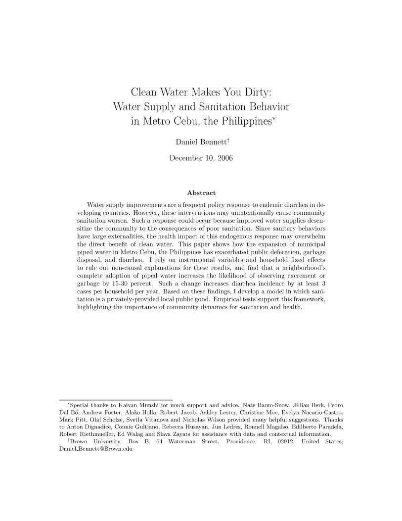
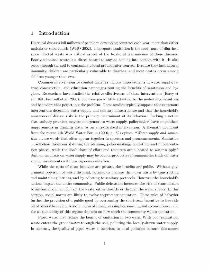
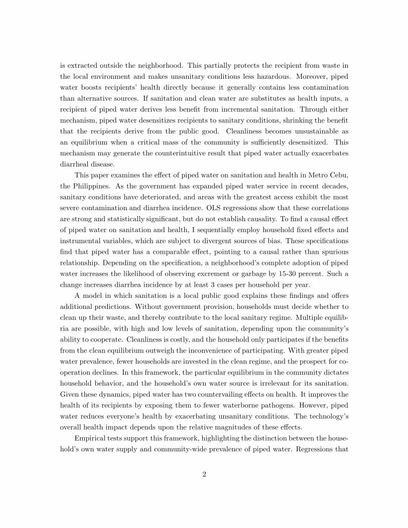
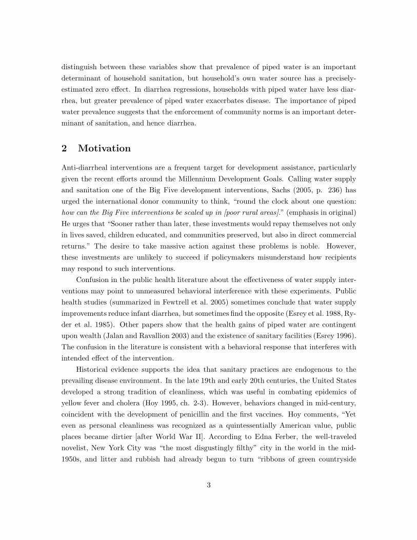
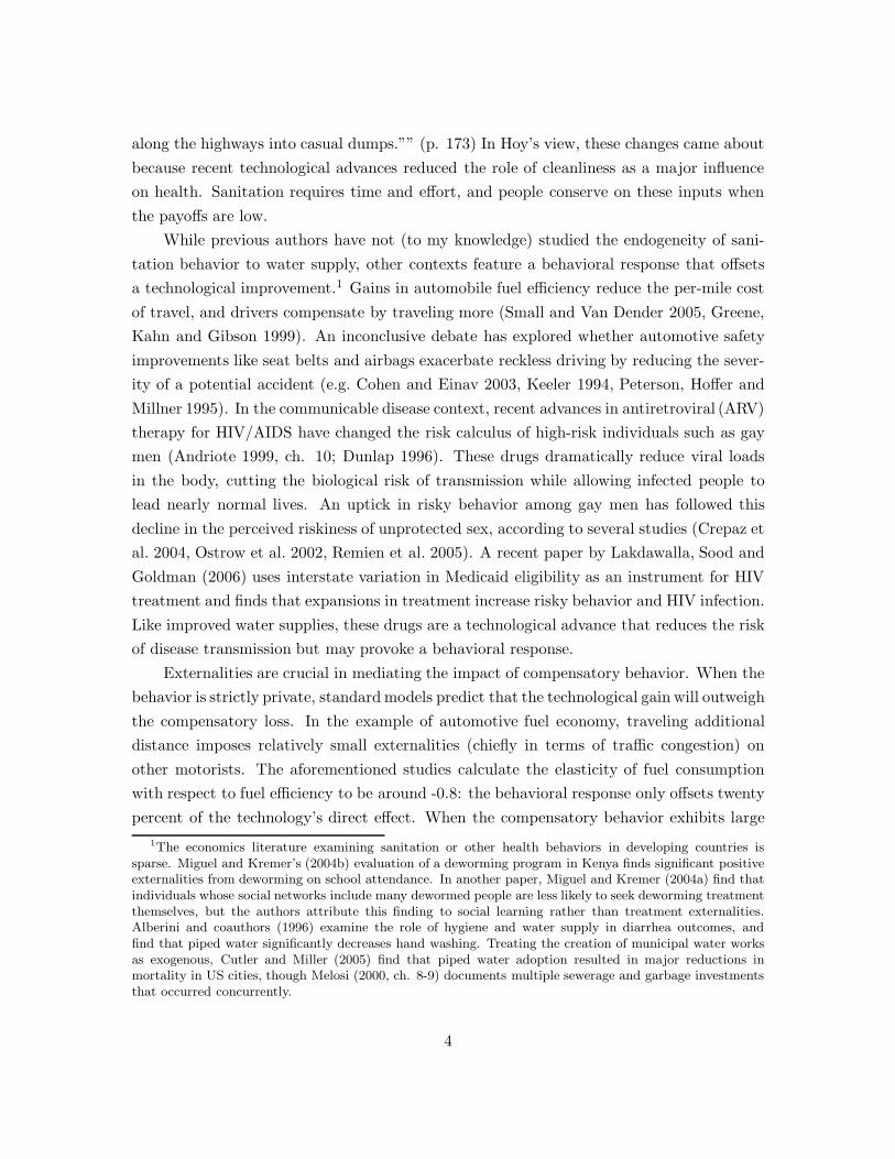
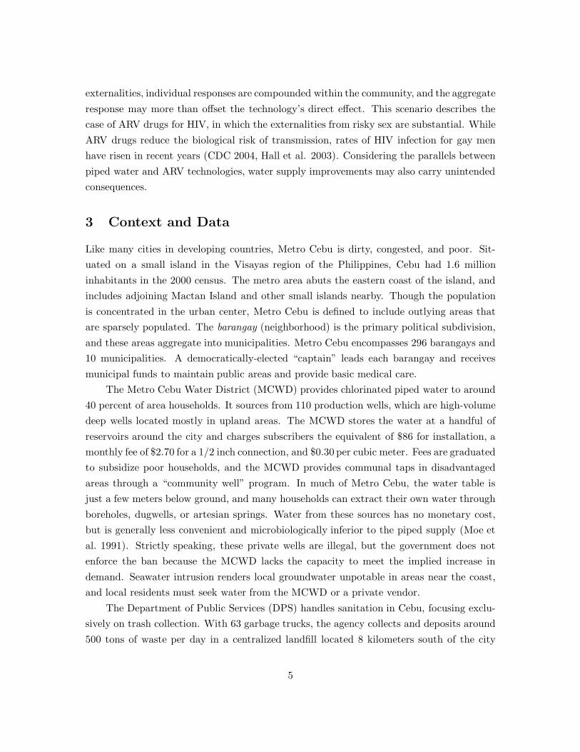
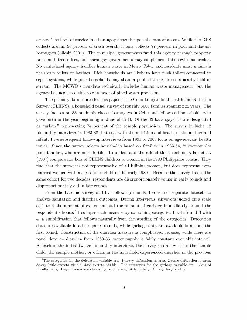
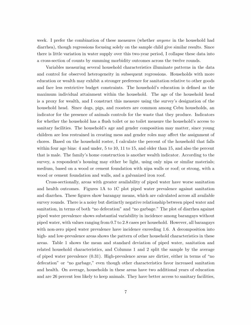
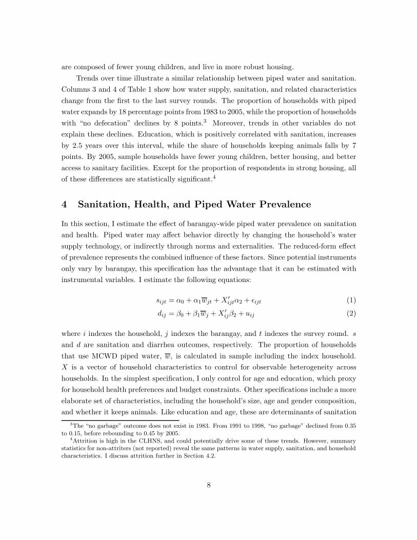
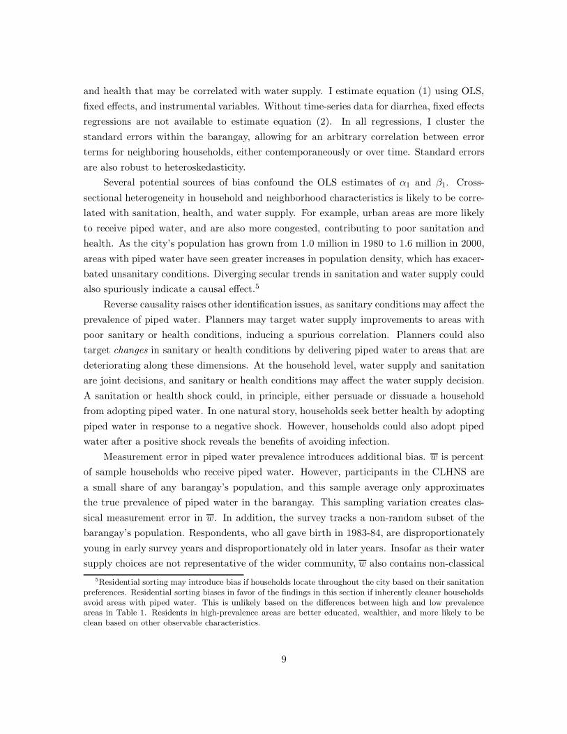
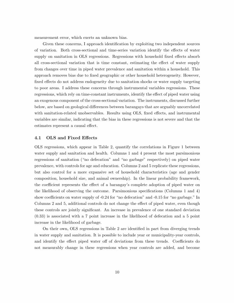
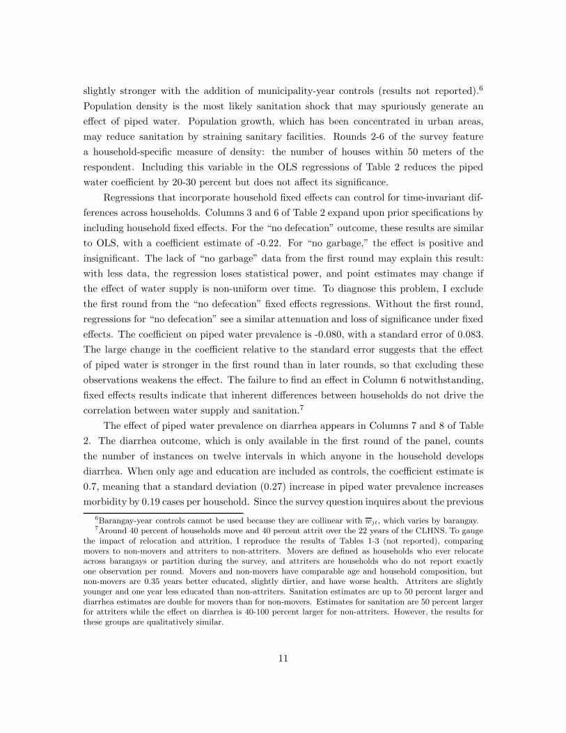
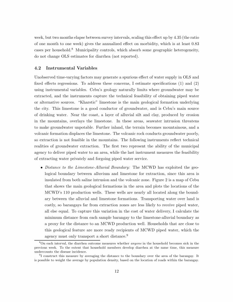
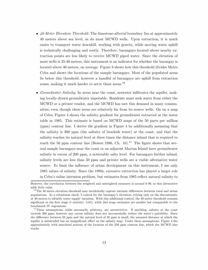
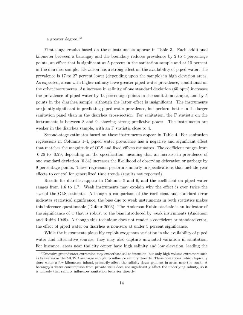
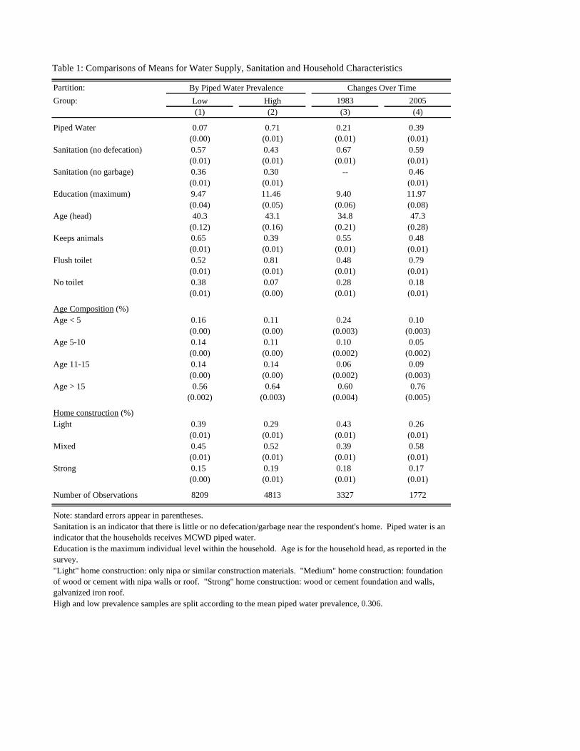
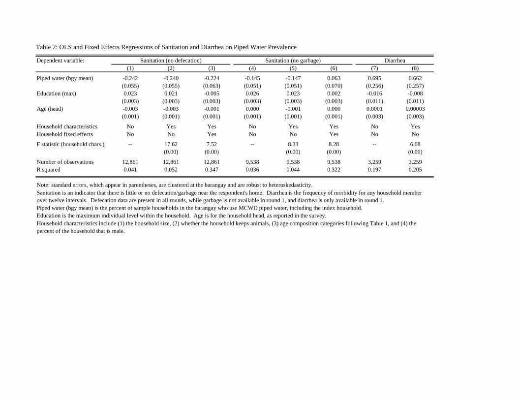
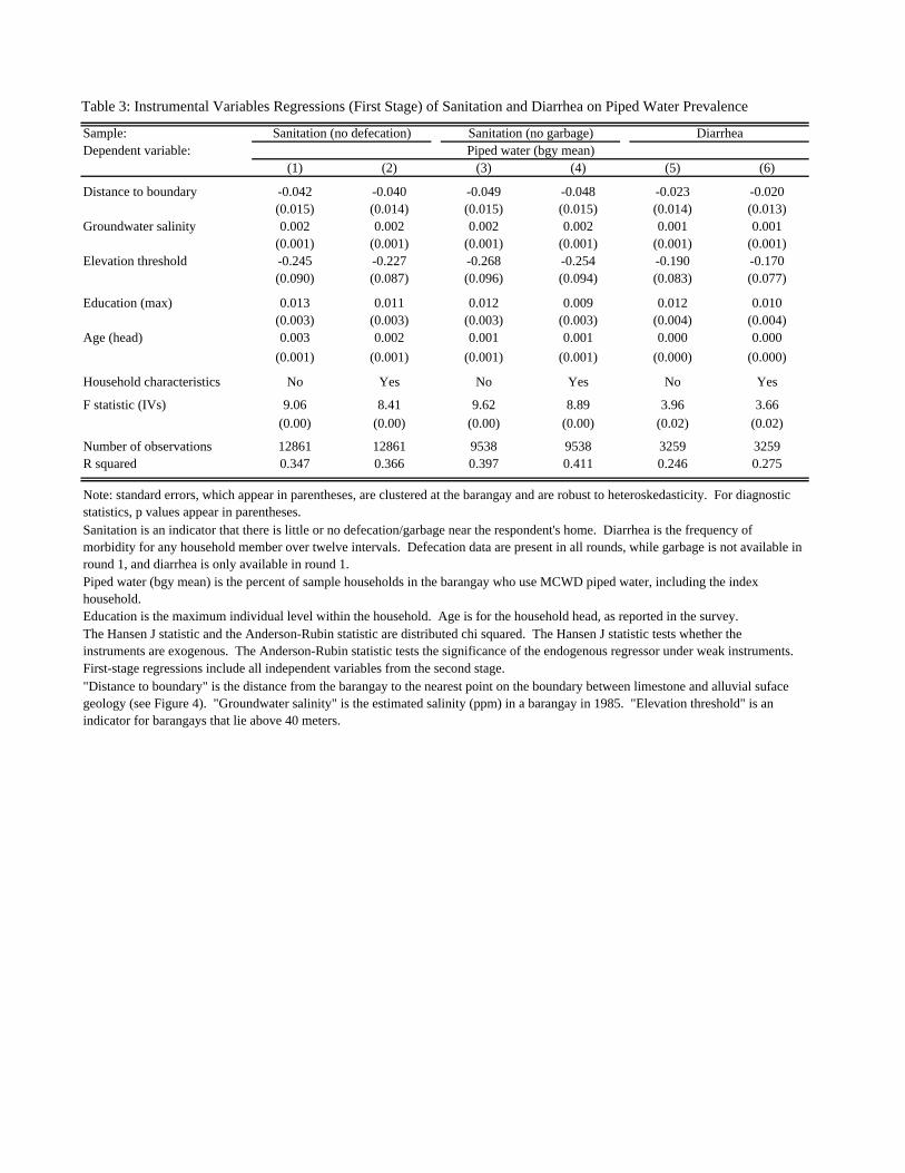
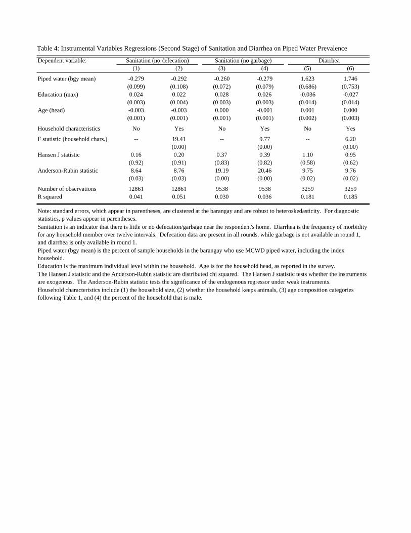
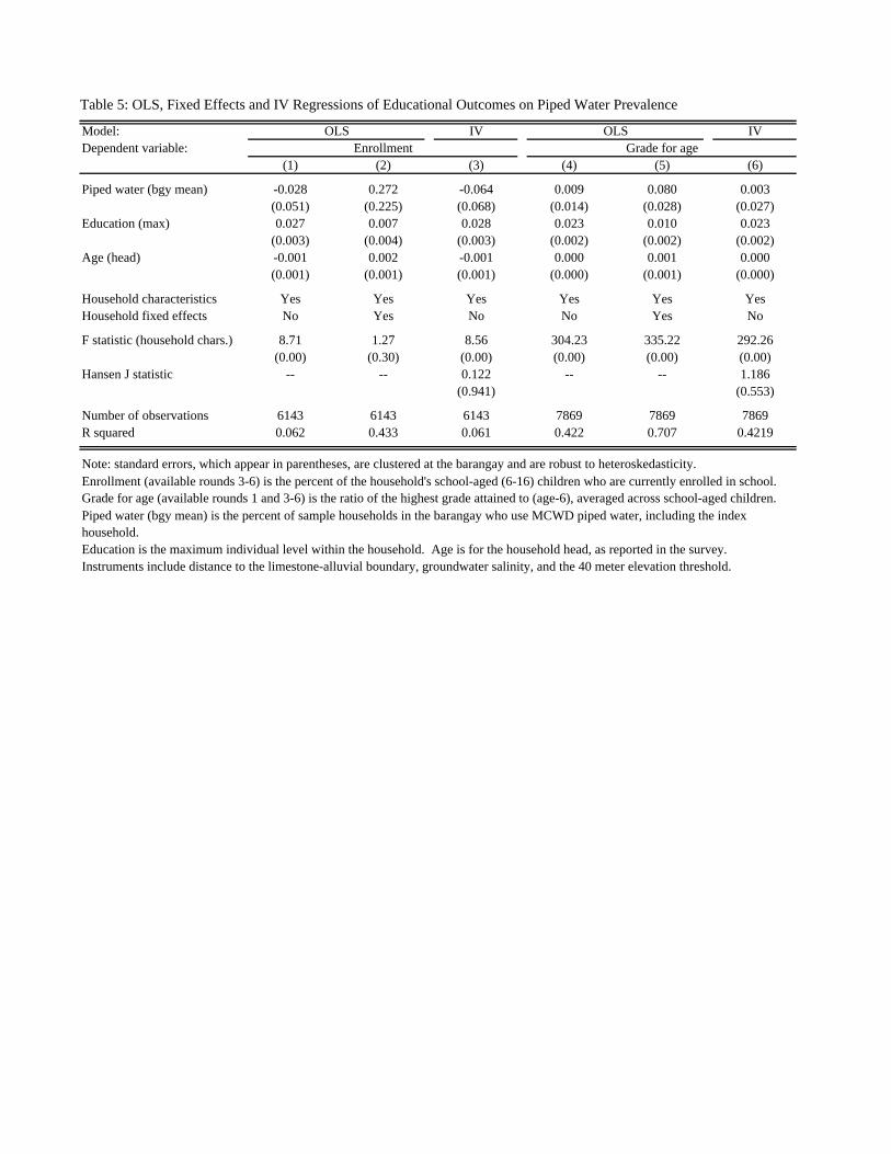
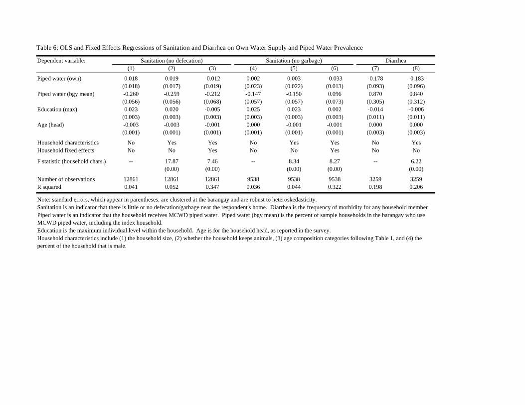
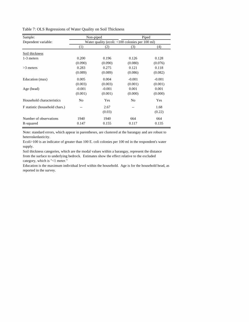
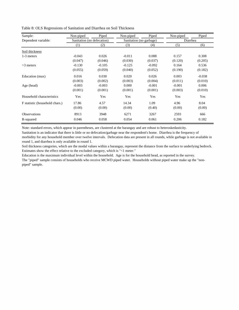
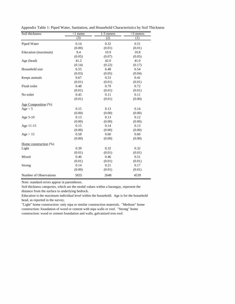
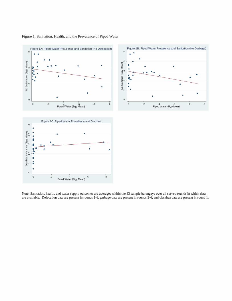
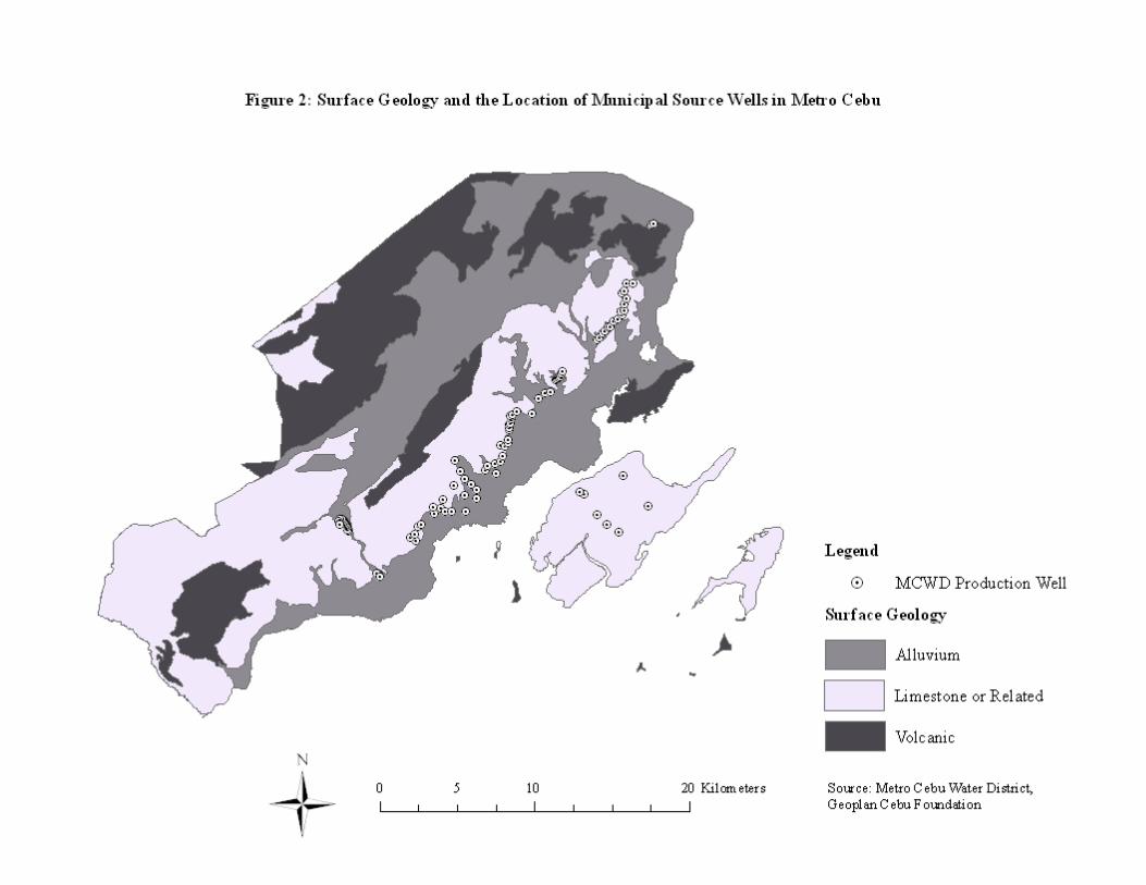
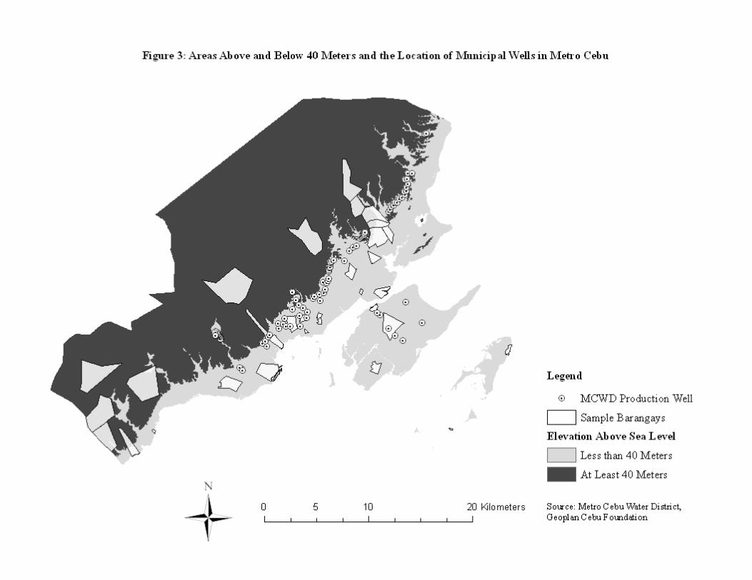
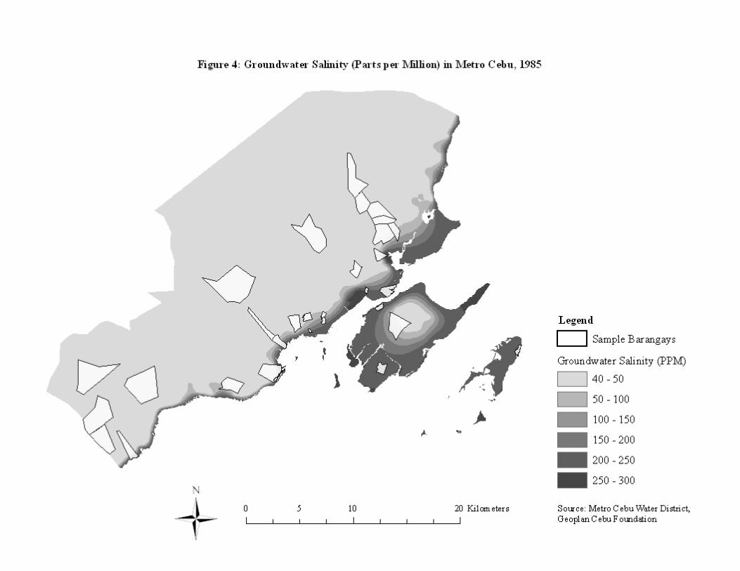


![Water,Sanitation,andHygieneServiceAvailabilityatRural ... · inadequate water supply and sanitation [3]. Inadequate drinking water, sanitation, and hygiene in nonhousehold settings,](https://static.documents.pub/doc/80x56/5e81efd69f9e151ba6551f5b/watersanitationandhygieneserviceavailabilityatrural-inadequate-water-supply.jpg)
