Robotics and Autonomous Systems 61 (2013) 1415–1439
Contents lists available at ScienceDirect
Robotics and Autonomous Systems
journal homepage: www.elsevier.com/locate/robot
Cleaning robot navigation using panoramic views and particle cloudsas landmarksRalf Möller ∗, Martin Krzykawski, Lorenz Gerstmayr-Hillen, Michael Horst, David Fleer,Janina de JongComputer Engineering, Faculty of Technology, Bielefeld University, D-33594 Bielefeld, GermanyCenter of Excellence ‘‘Cognitive Interaction Technology’’, Bielefeld University, D-33594 Bielefeld, Germany
h i g h l i g h t s
• A visually guided cleaning robot moves on meandering lanes even under odometry noise.• A topo-metric map with panoramic images and particle clouds in its nodes is built.• A holistic homing method estimates direction and rotation from low-resolution images.• Position estimates are corrected by interrelating images and clouds of two map nodes.• Complex environments can be covered by multiple adjoining meander parts.
a r t i c l e i n f o
Article history:Received 11 January 2013Received in revised form12 July 2013Accepted 26 July 2013Available online 3 August 2013
The paper describes a visual method for the navigation of autonomous floor-cleaning robots. Themethod constructs a topological map with metrical information where place nodes are characterized bypanoramic images and by particle clouds representing position estimates. Current image and position es-timate of the robot are interrelated to landmark images and position estimates stored in the map nodesthrough a holistic visual homing method which provides bearing and orientation estimates. Based onthese estimates, a position estimate of the robot is updated by a particle filter. The robot’s position esti-mates are used to guide the robot along parallel, meandering lanes and are also assigned to newly createdmap nodes which later serve as landmarks. Computer simulations and robot experiments confirm thatthe robot position estimate obtained by this method is sufficiently accurate to keep the robot on parallellanes, even in the presence of large random and systematic odometry errors. This ensures an efficientcleaning behavior with almost complete coverage of a rectangular area and only small repeated cover-age. Furthermore, the topological-metrical map can be used to completely cover rooms or apartments bymultiple meander parts.
This paper addresses the question of how an autonomous floor-cleaning robot can efficiently cover an area by parallel, mean-dering lanes. For this application, a controller keeps the distancebetween the lanes at a predefined value which usually corre-sponds to the width of the cleaning orifice (suction port), such thatfloor coverage per traveled distance on the lanes will be maximalwhile repeated coverage will ideally be avoided. Our approach isbased on the visual input from a panoramic camera system andstores panoramic images and position estimates in the nodes of atopological-metrical (topo-metric) map. The position estimate is
updated through a particle filter where the prediction step usesodometry information while the correction step uses bearing andorientation estimated from visual information. The latter are de-rived by interrelating the image of the current node to multipleviews stored at nodes on the previous lane which serve as land-marks. Bearing and orientation are estimated by min-warping, aholistic visual homing method specifically designed for panoramicimages. The current position estimate is fed into a controller whichkeeps the lane distance approximately constant.
We defer a detailed description of ourmethod until we have in-troduced the relevant concepts and recapitulated the current stateof the research. In Section 1.1 we review the current state in aca-demic and commercial cleaning robots. Concepts relevant for nav-igation based on panoramic images are summarized in Section 1.2.We finally outline the method proposed here in Section 1.3. For amore detailed review of the state of the art, we refer to our recentpublication [1].
1416 R. Möller et al. / Robotics and Autonomous Systems 61 (2013) 1415–1439
1.1. Cleaning robots
As vacuum-cleaning is frequently seen as a boring and mono-tonous task for humans, cleaning robots have been developedwhich are capable of autonomously cleaning a room or even an en-tire apartment. In the followingwewill briefly describe the currentstate of cleaning robots developed by commercial companies (Sec-tion 1.1.1) and by academic research institutions (Section 1.1.2).
1.1.1. Commercial cleaning robotsCommercial floor-cleaning robots for household usage have
been available on the market for approximately ten years. First-generation robots rely on preprogrammed movement patterns oron random-walk strategies. Achieving complete coverage requiresa relatively large amount of time and results in a large proportionof repeated coverage [2]. With their limited sensor equipment andwith limited computational power, these robots are not capable ofbuilding a representation of their workspace which would allowthem to distinguish covered areas from areas which still need tobe cleaned [3]. Several robots of this class were or are still availableon themarket (e.g. iRobot Roomba 531, 555, 564 PET, 581, 625 and780; Kärcher RC3000).
Second-generation robots rely on systematic exploration strate-gies and can recognize and directly approach uncleaned areas. Thisallows a robot to cover its workspace more efficiently and with asmaller proportion of repeated coverage. All of these robots knownto us move on meandering trajectories. Although little is knownabout the navigation strategies of these robots, it is clear that theybuild some kind of map of their workspace. Second-generationrobots have been available since around 2008; some are equippedwith a 360° laser range finder (e.g. Neato XV-11, XV-15, XV-25;Vorwerk Kobold VR100), others with amonocular camera directedtowards the ceiling (e.g. LGHombot 2.0; SamsungNavibot SR-8855and SR-8895 Silencio; Philips HomeRun FC9910).
1.1.2. Academic research on cleaning robotsIn contrast to the fast advances in the commercial sector, au-
tonomous floor cleaning robots have only received relatively littleattention in academic research. In the following,wediscuss the fewpapers specifically addressing control of floor cleaning robots.
Even though not directly related to the work presented here,we want to mention complete coverage planning algorithms forplanning paths to completely cover the robot’s workspace whileminimizing the portion of repeated coverage [2,4–8]. These papersmostly address the high-level problem of completely coveringcomplex-shaped workspaces such as entire rooms or apartments— a problem not covered in this paper but only mentioned as anextension of ourmethod in the outlook in Section 10. Those papersdealing with low-level aspect of cleaning-robot control as in thispaper present methods relying on range information rather thanon images and using localization andmap buildingmethodswhichbear no closer similarities to our method.
SLAM algorithms localize the robot within a map while simul-taneously building a map of the robot’s environment (textbooks:[9–11]). By integrating sensor data over time, themap is iterativelyupdated by applying a Bayesian filter framework. In the following,we focus on visual SLAM methods (as the method described herealso mainly relies on visual information) in the context of cleaningrobots.
The methods proposed by Jeong and Lee [12,13] use an ex-tendedKalman filter (EKF) for estimating the positions of robot andlandmarks. Visual input comes from a camera directed upwards.From the image of the ceiling and adjacent wall regions, SIFT [14]and line features are extracted as landmarks. The robot positionestimate obtained from the EKF is used to guide the robot on me-andering lanes. The method was extended to multi-robot SLAM
using a particle filter for state estimation [15,16]. Figures andsupplemental videos suggest that the Samsung robots mentionedabove use SLAM algorithms developed by this research group. Amethod also based on a ceiling camera is presented by Lee and Lee[17]; here orthogonal lines are used for correcting the robot orien-tation estimate while point features are matched for localization.
The SLAM method proposed by Choi et al. [18] relies on amonocular camera pointing into the robot’s direction of travel.The robot’s current state and the 3D positions of surrounding fea-tures are estimated by an EKF framework. The method is capableof adding new feature positions without waiting for a secondmea-surement by initially assuming a large uncertainty along the fea-ture’s viewing direction (because the feature’s position along thisdirection cannot be computed from a single image). The uncer-tainty is later on reduced if the feature is seen from a different po-sition.
Kwon et al. [19] propose a low-dimensional feature descriptorfor corner features and demonstrate the method in the contextof robot cleaning. They use a database of known features on theceiling, each associated with the feature position, for Monte Carlolocalization (thus performing no SLAM, but only localization).
1.2. Omnidirectional visual navigation
For our research on the navigation of cleaning robots, we use acustom-built robot equipped with an omnidirectional vision setup(Fig. 6). With this setup, we do not use image information from theceiling, but only consider the region around the horizon, since weexpect that the multitude of objects (e.g. furniture) visible thereoffers more visual structure than the ceiling. The advantages of asingle-camera system with a panoramic lens are that the robot iscapable of capturing a 360° viewof its environmentwith only a sin-gle camera, that rotational and translational motion componentscan be easily separated [20], and that the visible image content isindependent of the robot’s orientation.
Approaches to (omnidirectional) visual navigation can becoarsely categorized into model-based and appearance-based ap-proaches [21, chapter 3.6]. In the former case, the map is a geo-metrical model of the robot’s environment, and building themodelrequires to estimate the spatial position of visible objects. To cir-cumvent the computational effort for estimating the spatial posi-tions of visible objects, appearance-based methods solely rely onintensity information or information directly derived from the in-tensity. The following review section focuses on appearance-basedtechniques because the navigation strategies proposed in this pa-per belong to this class.
1.2.1. Model-based navigation methodsThe core of all model-based navigation methods is to compute
a 2D or 3D model of the environment which is used as map. Vis-ible objects are in most cases represented by interest points (re-view: [22,23]), and position estimates are computed and updatedby probabilistic frameworks (e.g. Kalman filters or particle filters,textbooks [9,10]) or by optimization techniques (e.g. graph-basedSLAM or bundle adjustment, reviews: [24,25]). The main difficultyof building and updatingmodel-basedmaps is to localize the robotbased on uncertain landmark estimates, and to update landmarkestimates based on noisy sensor measurements taken from an un-certain robot position. Since the spatial positions of features aredetermined, model-based maps can be easily visualized. Never-theless, interpreting the map can be difficult for a human user ifthe map consists of a relatively small number of feature pointsdistributed sparsely over the robot’s workspace. Since monocularomnidirectional cameras are bearing-only sensors, it is only pos-sible to compute the direction of a visible feature, but not its dis-tance. With amonocular setup, computing the distance requires at
R. Möller et al. / Robotics and Autonomous Systems 61 (2013) 1415–1439 1417
least two images taken at different robot positions. Only omnidi-rectional stereo setups (e.g. [26,27]) can compute a feature’s dis-tance with only one camera image, but these are rarely used formap-based navigation.
In the context of classical feature-based SLAM (tutorial [28])with monocular omnidirectional cameras, the methods by [29,30]use a delayed update scheme where an observed feature is onlyadded to the map as soon as it has been observed a second timesuch that its location can be obtained by triangulation. In the caseof loop closures, i.e. repeated observations of a feature at a laterpoint in time, the estimate of the feature’s spatial position is re-fined. For efficient loop-closure detection, the method of [29] usesan appearance-based technique, namely histogram comparisons.The visual feature-based SLAM methods reviewed in Section 1.1.2all maintain a model-based map of the robot’s environment.
Visual odometry methods (reviews: [31,32]) focus on comput-ing an accurate estimate of the robot’s current position. This isachieved by estimating the robot’s motion between consecutivecamera images and updating the position estimate accordingly.The environment model is rather a byproduct of the motion-estimation process (e.g. [33–37]). Visual odometry is especiallysuited for omnidirectional images since it is easier to disambiguatetranslation from rotation than with standard camera images. Incontrast to feature-based SLAM methods, visual odometry meth-ods usually do not detect loop closures and do not subsequentlycorrect position estimates. Exceptions include the methods in[36,35] which also use appearance-based loop-closure detectionmethods, namely bag-of-word approaches based on vocabularytrees.
1.2.2. Appearance-based navigation methodsAppearance-based navigation strategies avoid the effort for es-
timating and maintaining the spatial positions of visible objects.They rather use the raw image-intensity information the robotperceives when visiting a place for navigation. Integrating severalplaces into a map directly leads to a graph-based representationof the robot’s environment, usually referred to as topological map.Such maps represent places as nodes in a graph; spatial interrela-tions aremodeled by edges representing reachability between twoplaces. To each node, the sensory information the robot perceivedat the corresponding place is attached.
Topological maps can be further categorized into purely topo-logical maps and topo-metric maps [21, chapter 3.6]. The former arequalitative maps which do not contain metrical position informa-tion; the latter are quantitative maps which store in each node ofthe map the sensory information perceived at the correspondingplace together with an estimate of the robot’s position at this pointin time. Both types of topological maps are typically a sparse rep-resentation of space (though not in our method, Section 1.3) withnodes strategically placed at important locations or at a distanceas large as the node-to-node navigation method (e.g. local visualhoming, see below) tolerates.Purely topological maps. Since they do not containmetrical positionestimates (neither of visible features as is the case formodel-basedmaps nor of former robot positions as is the case for topo-metricmaps), purely topological maps can be more easily constructedthan other map types. While purely topological maps allow for lo-calization only with respect to the closest node in the map, localnavigation methods (e.g. local visual homing, see below) can nev-ertheless guide the robot fromnode tonode such that all previouslyvisited places in the map can be reached. Purely topological mapshave the disadvantages (i) that maps cannot be visualized for theuser in the usual metrical form (which, in the cleaning robot ap-plication, may be required for user interaction, e.g. the selection ofareas to be cleaned), (ii) that navigation in topological maps mayrequire additional information if different places in space have the
same visual appearance (spatial aliasing), and (iii) that shortcutsbetween nodes without a common edge are not possible.Topo-metric maps. Regarding the complexity required for con-structing and updating themap, topo-metricmaps are a good com-promise between the simplicity of purely topological maps andthe complexity of model-based maps. Storing an estimate of therobot’s position in the place node allows for continuous localiza-tion and increases the robustness against spatial aliasing: placeswith identical visual appearance can be distinguished based ontheir position estimates. Moreover, nodes can be visualized to-gether with other information (e.g. obstacle points obtained fromrange finders) in a human-readable map. Thus, they combine theadvantages of topological and model-based maps. Therefore, andsince the movement on parallel lanes requires metrical informa-tion, the method proposed in this paper relies on a topo-metricmap.
Topo-metric maps are frequently used in conjunction withtrajectory-based SLAM methods (tutorial: [38, sec. IV.D]). Amongall SLAMmethods, trajectory-basedmethods have the closest sim-ilarity to our method (see also our preliminary experiments witha trajectory-based SLAM method in Section 10.3). While feature-based SLAM methods (tutorial: [28]) estimate the positions of ex-ternal landmarks, trajectory-based SLAMmethods interpret formerrobot positions as landmarks. According to [38], trajectory-basedSLAM methods are suited to environments where a direct align-ment of the sensory data collected at two locations is easier thana detection of isolated landmarks. Although originally proposedfor standard cameras (e.g. [39,40]), trajectory-based SLAM is of-ten used with omnidirectional images [41–46]. In these methods,robot positions are characterized by omnidirectional (panoramic)images which are stored in the nodes of a topo-metric map. Linksbetween adjacent place nodes of themap are annotatedwith infor-mation derived from partially estimating the robot’s ego-motionbetween the corresponding nodes. Such partial ego-motion esti-mates include (i) an odometry-based estimate of the traveled dis-tance, (ii) an estimate of the robot’s change of orientation obtainedfrom a visual compass, or (iii) bearing information, e.g. obtainedfrom local visual homing (Section 1.2.2). Since the angular rela-tions obtained from compass and bearing measurements only de-fine spatial relations up to scale, all methods require somemetricaldistance information. All methods we are aware of obtain this es-timate from the robot’s wheel odometry. Aspects (ii) and (iii) areusually solved by vision-based ego-motion estimation techniquesrelated to local visual homing and will be discussed below.
Trajectory-based SLAM methods update and correct the topo-metric map based on the position information and the spatialrelations attached to the nodes and the links of the graph, respec-tively. Depending on how these operations are performed, onecan distinguish between probabilistic methods and optimization-based methods (see e.g. [47,9]). Probabilistic methods correct themap by estimating the most likely configuration depending on thegiven sensor information. Trajectory-based SLAMmethods for on-line SLAM (i.e. methods updating the map whenever new sensordata is available) rely on Bayesian filtering techniques, namely onan extended Kalman filter (EKF, [44]) and on an exactly sparse ex-tended information filter (ESEIF, [45]) (textbook: [9]). These filter-ing techniques assume that the occurring probability densities areGaussian (in contrast to ourmethodwhich relies on a particle filterapproximating arbitrary distributions by a particle cloud). In a pa-per by Rybski et al. [44], another method is proposed relying on amaximum likelihood estimation for offline SLAM (i.e. for estimat-ing the map after collecting all sensor data).
The methods by Andreasson et al. [41,42], Rybski et al. [43],Hübner and Mallot [46] belong to the class of optimization-basedSLAM methods. Such approaches transform the spatial relationsstored in themap into a set of constrained equations and search for
1418 R. Möller et al. / Robotics and Autonomous Systems 61 (2013) 1415–1439
the best fitting map configuration by error minimization. The opti-mization process is usually referred to as relaxation. The methodsdiffer in the applied optimization technique: multi-level relax-ation [41,42], relaxation of a mass–spring model [43], and multi-dimensional scaling [46].
Like for the classical feature-based SLAM algorithms (Sec-tion 1.2.1), correct loop-closure detection is also essential fortrajectory-based SLAM methods. Since the robot’s position esti-mate can drift, loop-closure detection has to be a purely vision-based process and is therefore closely related to localization inpurely topological maps. A number of contributions address theproblem of localization and loop-closure detection based on om-nidirectional images. For this purpose, omnidirectional images areadvantageous since all features will be visible, regardless of therobot’s orientation. A classification of loop-closure approaches isgiven in [48]. The major problem is to find image representationswhich allow to perform a large number of image comparisons inshort time. Widely used are visual bag-of-word approaches basedon vocabulary trees (e.g. [36,35]): a feature vector is assigned toa single visual word (an integer value) in a quantization process.An image is then characterized by a sparse binary vector encodingwhich visualwords are present. A hierarchicalmethod for the com-parison of omnidirectional images is suggested in [49]: A dynami-cally changing set of key images is selected from themapby a graphapproach, and a new image is only compared to these key images inthe first stage of the hierarchicalmethod. Coarse position estimatesobtained by imagematching can be refined by using the Bayes rulewhen new images are captured [50]. In [51], the number of SIFT orSURF correspondences is used as distance measure for view-basedlocalization, with the specific goal to tolerate seasonal changes inthe appearance to improve the robustness of outdoor navigation.Local visual homing. Local visual homing algorithms are used fornode-to-node navigation in purely topological maps or for ego-motion estimation to derive spatial relations between nodes of atopo-metric map. In the context of this work, local visual homingis applied in the latter sense. The former application correspondsto the initial purpose of local visual homing, which is to allow arobot to approach a previously visited place under visual control.The goal location is characterized by a snapshot image capturedthere. By comparing the snapshot to the current view perceived bythe robot, a home vector pointing from the robot’s current positionto the goal position, and an angle expressing the azimuthal rotationof the camera between the two positions are computed. Thus,local visual homing can be seen as a partial solution of the ego-motion estimation problem (review: [52]), and it is closely relatedto visual servoing (review: [53]), to visual odometry (Section1.2.1 and reviews: [31,32]), and to image registration (reviews:[54,55]). Since two images captured at unknown locations areinterrelated, spatial relationships can only be estimated up to scale.This can either be done by extracting and matching a set of visiblefeatures (correspondencemethods) or by comparing entire images(holistic methods). Most correspondence methods derive bearingand compass information from estimating the two-view geometrybetween the considered images [43–45]. Only the method byAndreasson et al. [41,42] uses a relative image similarity measureinstead to avoid the effort for two-view geometry estimation. Forthe work presented in this paper, we rely on a holistic homingmethod referred to as min-warping (Section 2). A predecessor [56]of this methods is used by Hübner andMallot [46] in the context oftrajectory-based SLAM. For a recent review on local visual homingalgorithms, the reader is referred to Möller et al. [57].1 Visual
1 An interesting development not covered there is the ‘‘optical rails’’ methodsuggested in [58–60]; it is based on a gradient descent in image distances,accelerated by representing omnidirectional images through an expansion intospherical harmonics.
homing is possible in a limited range surrounding the goal position(catchment area); for long-range navigation, several snapshotsneed to be integrated into a topological map.
1.3. Proposed method
In this paper, we propose a method for covering a single rect-angular area with parallel andmeandering lanes. This is motivatedby the goal to clean the rectangular area completely and withmin-imal overlap of the opening of the suction port (cleaning orifice).Themethod can be extended to cover complexworkspaces bymul-tiple, adjoining parts of meandering lanes; we give an outlook inSection 10. As a spatial representation, the method builds a topo-metric map, and uses panoramic images to represent places; theadvantages of this combination have beenmentioned above. Topo-metric maps are usually sparse, but the cleaning problem calls fora dense map. While following a lane, place nodes are added to themap at approximately equal distances. Place nodes store the cur-rent panoramic image (called a snapshot) together with an esti-mate of the robot’s current position. The position is estimated bya particle filter, and thus all position estimates are particle clouds.The prediction step of the particle filter relies on the robot’s odom-etry. The correction step incorporates bearing and orientation in-formation obtained from interrelating the current view and severalsnapshots stored along the previous lane by means of local visualhoming.
Panoramic views stored at nodes on the previous lane togetherwith a position estimate in the form of a particle cloud are usedas landmarks (as indicated in the paper’s title). We think that us-ing entire views as landmarks mitigates the landmark associationproblem, since, first, entire views are usually more unique than lo-cal visual features (e.g. the surroundings of corners) as typicallyused by feature-based SLAM approaches, and, second, the identityof a view representing a landmark is known (in contrast to exter-nal landmark features where the identity of a landmark has to beestablished in the association process).2 A holistic local visual hom-ing method called min-warping estimates bearing and orientationfrom image pairs not by matching local visual features, but by es-sentially distorting one of the images according to a set of hypo-thetical robot movements and searching for the best match withthe other image. We prefer such holistic methods in contrast tomethods based on feature correspondences since holistic methodsexploit all available information by using the entire image ratherthan a set of local features, require only moderate preprocessing(no keypoint detection or feature extraction), and can work onsmall images with coarse resolution.
Since our method aims at an application on consumer clean-ing robots with limited computational capacity, we deliberatelydecided against using a full-scale SLAM approach. At least at thecurrent stage, we therefore do not update a position estimate againafter attaching it to its corresponding place node when this nodeis created. We will attempt to solve problems arising from the re-sulting position drift by explicitly employing visual loop closuredetection [61]. We think that this might be sufficient to avoid thata cleaning robot leaves out an area or cleans it multiple times. Loopclosure detection will not be addressed in this paper, however.
Nevertheless, the method bears similarities with trajectory-based SLAM methods (Section 1.2.2): it constructs a topo-metricmap of the environment during the cleaning run; robot locationsand the corresponding views serve as landmarks; and views stored
2 It should be pointed out, however, that spatial aliasing (e.g. in repetitiveenvironments like long corridors) can lead to errors since there can be locationswith views similar to one of the snapshots stored in the map, and bearing andorientation estimates may erroneously relate to these ‘‘ghost’’ snapshots.
R. Möller et al. / Robotics and Autonomous Systems 61 (2013) 1415–1439 1419
in the map are used to determine spatial relationships betweena new node and nodes in the map. Our method is related toprobabilistic trajectory-based SLAM methods but interrelatesparticle clouds (Section 3.3) rather than multivariate Gaussians. Itis using a simple but robust holistic homing method whereas themajority of trajectory-based SLAMapproaches are based on featurecorrespondences. Specific for the cleaning task is that landmarkviews are taken from the previous lane according to differentselection schemes (Section 8.2), since the goal is to guide the robotalong parallel and meandering lanes.
The method described in this paper takes up some basic ideasof our earlier work [62,63,1]. In the most recent of these previ-ous methods [1], movement on parallel lanes was accomplishedin a deterministic framework where uncertainties of home vectorand compass estimates and of the robot and landmark positionestimates were not considered. Moreover, only a partial positionestimate (orientation and distance to the previous lane) was main-tained. This position estimate was updated through triangulationof landmark locations on the previous lane (using a local visualhoming method as well). The method presented in this paper onlycopies the ideas (1) to use local visual homingwith landmark viewson the previous lane for updating the position estimate, (2) to useof a topological-metricalmap rather than ametricalmap, and (3) toexplore whether the cleaning task can be accomplished without afull-scale SLAM approach. The rest of our novelmethod differs fun-damentally from our earlier work (andwas implemented indepen-dently). It uses a probabilistic framework based on the particle filterwhich takes uncertainties ofmeasurements and position estimatesinto account. Moreover, the transition to full position estimates(two spatial, one angular coordinate) considerably simplifies thedevelopment of methods capable of covering the entire workspaceby adjoining parts ofmeandering lanes (comparable to the iterativeconstruction of a scaffold) aswell as the integration of range-sensormaps required for free-space detection (see outlook in Section 10)— here our previous method may have overdone the simplifica-tion by only using a partial position estimate. Instead of triangula-tion, the novel method uses superposition of multiple measurementsbased on local visual homing in the correction step of the particlefilter which we consider to be a much more general approach.
Both here and in our earlier work we demonstrate that a rela-tively simple map-building and localization method can maintaina position estimate which is sufficiently robust to keep the roboton parallel lanes, even in the presence of strong random and sys-tematic odometry errors. We will show in the outlook (Section 10)that our novel method can be extended such that an entire roomor apartment is cleaned. Our attempt to stick to the simplest possi-ble method is mainly motivated by the limited onboard computerpowerwhich can be provided on consumer cleaning robots.We areaware that moving a cleaning robot on parallel lanes can also beaccomplished with even smaller effort by using odometry (whichshould be sufficiently reliable at least on hard floor) together witha cheap inertial compass sensor. However, such an approach isseverely limited in its application range: First, such a method can-not tolerate unexpected changes of the robot position (‘‘kidnappedrobot’’). Such changes can be tolerated by our method as long asthe robot is in the vicinity of an area covered by its map (e.g. bycoarsely localizing itself by image comparisons and then refiningthe position estimate by local visual homing). Second, the positionestimate drifts over long cleaning runs due to odometry errors anddrift of the inertial compass.While drift cannot be completely com-pensated in our non-SLAM approach, the robot can always localizeitself with respect to themap, even if themap is notmetrically con-sistent, and can therefore never get lost. Third, the low precision ofthe position estimate obtained by odometry and inertial compassprevents an extension with methods for user interaction, e.g. formarking areas to be cleaned or to be excluded— in the next run, the
robot position estimate differs from the one used to mark the area.Using an image-based approach ensures that the marked area canbe recognized (as long as the visual appearance has not changeddrastically).
The remainder of this paper is structured as follows. Section 2briefly recapitulates the local visual homing method which is thebasis of our navigationmethod. The application of the particle filteris described in Section 3. Section 4 presents the meander strategyand the controller. The method is tested in simulations (Section 5)and using our custom-build cleaning robot in the shape of a com-mercial, domestic cleaning robot (Section 6). The performanceis quantitatively assessed based on five evaluation measures de-scribed in Section 7. Experiments and results are presented in Sec-tion 8. A discussion (Section 9) and conclusions with an outlook tofuture work (Section 10) conclude the paper.
2. Local visual homing method: min-warping
In the following we briefly outline the local visual homingmethod ‘‘min-warping’’ used in the experiments described in thiswork. For details, the reader is referred to Möller [64] and Mölleret al. [57]. Please note that min-warping could be replaced by anymethod which can produce a home vector and a compass esti-mate from two panoramic images. We prefer min-warping sincethe method was developed in our group and we have the most ex-perience with it.
Min-warping [57] was created in the framework of the imagewarping method [56] which we extended from one-dimensionalto two-dimensional images [64]. Warping methods belong to theclass of holistic homing methods where the entire image is con-sidered, in contrast to correspondence methods where correspon-dences between selected local features from the two images areestablished. An advantage of min-warping and other warpingmethods is that no complex feature detection is required – imagecolumns are the features matched between the two images – andthat the resolution of the matched images can be relatively coarse(here 1°).
All warping methods, including min-warping, explicitly searchthrough a space ofmovement parameters. Given a panoramic viewat a reference location (called ‘‘snapshot’’) and a current view atanother location, min-warping tries to find movement parameters(direction of movement and orientation change) which would dis-tort (‘‘warp’’) the snapshot in a way that it matches best with thecurrent view. The best-fitting movement parameters yield bothan estimate of the angle of the home vector (pointing from thecurrent location to the reference location) and an estimate of theorientation difference between the two panoramic images (calledvisual compass). In extensive tests on image databases, warpingmethodswere shown to produce precise home vector and compassestimates in large regions around the reference location [64,57];min-warping is among the best methods [57]. Scaramuzza et al.[65, sec. 4] point out that a holistic (‘‘appearance-based’’) visualcompass for panoramic images [66,67] workedmore robustly thana feature-basedmethodwhich turned out to be sensitive to calibra-tion errors. Since such a holistic visual compass is integral part ofmin-warping, we are optimistic that min-warping is competitiveto feature-based local visual homing (or ‘‘ego-motion estimation’’)techniques; however, a direct comparison is presently not avail-able.
Min-warping operates on two-dimensional panoramic images.In such an image, horizontal pixel coordinates vary with theazimuth of the gaze direction while vertical pixel coordinates varywith the elevation (example images are shown in Fig. 9). Min-warping rests on a so-called ‘‘equal-distance assumption’’ statingthat all pixels in a given vertical image columnbelong to landmarksin the real world which have the same ground distance from
1420 R. Möller et al. / Robotics and Autonomous Systems 61 (2013) 1415–1439
Fig. 1. Min-warping, top view of the plane in which the robot is moving. Apanoramic reference image (snapshot) is captured at S; the robot’s orientation atS is indicated by the thick arrow. A simulated movement in direction α and withorientation changeψ anddistance d is executed. After the simulatedmovement, therobot is located at the current position C and assumes the orientation indicated bythe thick arrow. A landmark at L (here represented by a pixel column of a panoramicimage) appears under an azimuthal angle α+ x in the snapshot, and under an angleα−ψ+x+y in the current view. Since neither the distances to the landmark (r , r ′)nor the covered distance d are known, the landmark could be located at all positionon the beam originating at S (indicated by three example locations). Min-warpingsearches for best-matching image columns over a range of the angle y (indicated bythree example angles).
the snapshot location; however, this distance may differ betweencolumns. Since only static, monocular images are captured, thelandmark distances are unknown.
Fig. 1 explains the basic idea of the method; the details aredescribed by Möller et al. [57]. The snapshot was captured at thereference location S in the orientation indicated by the thick arrow.Min-warping searches through all movement parameters (α, ψ)which describe the direction of the hypotheticalmovement (α) andthe change in orientation (ψ) relative to the robot’s orientation atthe reference location S. Given these movement parameters, themethod assumes that the current viewwas captured from locationC in the orientation indicated by the thick arrow. The distance dbetween S and C is unknown.
Min-warping determines how good the current view fits to thehypothesis that it was actually captured from the hypotheticallocation C. For each landmark (an image column) which, seen fromS, appears under the angle x+α relative to themovement direction,min-warping searches through all possible locations L where thislandmark column may appear in the current view. Seen from C,the landmark appears under an angle α − ψ + x + y relative tothe robot’s hypothetical orientation at C. For x ∈ [0, π], the angley varies in the interval [0, π − x]; for x ∈ [−π, 0], it varies in theinterval [−π−x, 0]. Min-warping compares the landmark columnin the snapshot (azimuth angle α + x) with the landmark columnin the current view (azimuth angle α − ψ + x + y).
Since the hypothetical movement of the robot also affects thevertical scaling of the column, either the snapshot column or thecurrent view columnhas to bemagnified around the image horizonbefore the columns can be compared. Given x and y, the scale factorσ for the magnification can be computed from the ratio of thelandmark distances
σ =r ′
r=
sin xsin(x + y)
(1)
(law of sines applied to triangle LSC); here, r is the unknowndistance of the landmark L from the reference location S, and r ′ isthe unknown distance of L from the hypothetical current location
C. Note that although both the distance r and the distance r ′ areunknown, we can compute their ratio σ from x and y, and this ratiodetermines the magnification factor for the image columns.
The minimal distance measure (see below) between the imagecolumns found over y for each angle x is accumulated. The sum de-scribes how good the current view matches under the hypothesisthat it was captured from C, and ultimately how good the move-ment parameters (α, ψ) correspond to the true movement of therobot. Themovement parameters (α, ψ) for which the sum ismin-imal are the result of the method. The angle of the home vector(pointing from C to S) relative to the current orientation of therobot is determined from β = α− ψ +π , the compass angle is ψ .
As the distance measure between two image columns, denotedby vectors a and b, we use the partly illumination-invariant mea-sure J defined by
The first term compares the columns according to their vectorlength (essentially comparing their overall intensity). The distancemeasure in the second term is fully invariant against multiplica-tive changes in intensity. In experiments on image databases (datanot shown here) we foundw = 0.1 to be the optimal weight. Notethat, this gives stronger weight to the illumination-invariant sec-ond term compared to the Euclidean distance (used by [57]) whichwe obtain as a special case forw = 1/3.
The search space is discretized in 72 steps in each movementdimension (α and ψ , both varying in [0, 2π)). Since the verticalscaling of image columns and the comparison of columns are time-consuming, the actual implementation of min-warping precom-putes distances between image columns scaled according to a setof discrete scale parameters. Here we use the scale parameter set{0.4, 0.5, 0.625, 0.8, 1.0, 1.25, 1.6, 2.0, 2.5}. A set of thresholdsdefines which precomputed distance to select; here the thresholdset is {0.0, 0.45, 0.56, 0.71, 0.9, 1.12, 1.42, 1.8, 2.25, 3.0} (e.g. fora value σ = 0.694 computed from (1) which lies in the interval[0.56, 0.71] we use the precomputed distances for the scale fac-tor 0.625). These sets were chosen experimentally in pure homingexperiments on image databases. The scale factors are inversion-symmetrical such that both images are magnified by the same fac-tors. The maximal magnification (0.4, 1/2.5) should not exceed acertain value since otherwise the loss of image structure increasesthe danger of mismatches. The resolution of the scale factor setis sufficiently fine such that a good match between the imagecolumns (corresponding to the same feature in the world) isachieved even if the true scale factor lies between the values in theset. The thresholds lie approximately in the center between twoneighboring scale factors they separate.
We accelerate the method by limiting the search ranges of theα and ψ parameters to a range of ±π/4 around estimated valuesof α and ψ which are determined from the estimated current andreference positions. This reduces the computation time to less than10 ms for an image size of 360×30 in an integer-based implemen-tation using SSE2 SIMD instructions on a modern Intel CPU (i7).
3. Application of the particle filter
The particle filter is implemented in the standard way (seetextbooks: [9,68,11]). In total M = 100 particles are used in allour experiments. Each particle i has four components: the robotposition xi = (xi, yi, θi) in the horizontal plane, and the importancefactor (weight) wi which is modified in the correction step andconsulted in the resampling process. In our application, particleclouds do not only represent the robot position, but also thepositions of landmarks. When a landmark is created, the particlecloud representing the current robot position is stored together
R. Möller et al. / Robotics and Autonomous Systems 61 (2013) 1415–1439 1421
with a panoramic image captured at this position.When a homing-based correction step is later applied, the current particle cloud andthe current image are related to the landmark’s particle cloud andthe landmark image (also called ‘‘reference image’’ or ‘‘snapshot’’).In the following we describe the steps of the particle filter:initialization, prediction, correction (computation of importancefactors by either using visual homing methods or data from rangesensors), and resampling (which is the same for each correctionscheme).
3.1. Initialization
It is assumed that the initial position of the robot is known. Thisis justified in our case since a cleaning robot will typically start ata charging station with fixed position. The initial position estimateof the robot is assigned to all particles.
3.2. Prediction
In our straightforward implementation of the prediction step,we use the odometry equations provided by Siegwart and Nour-bakhsh [10] (there sec. 5.2.4) for a robot with differential steering.Let xi = (xi, yi, θi) be the previous position estimate representedby particle i, and ∆s = (∆sl,∆sr) the distances covered by leftand right wheel since the last measurement. We compute a newposition estimate from x′
i = f(xi,∆s), and the corresponding un-certainty (represented by a covariance matrix) is updated throughan error propagation process by
Cx′i= FxiCxiF
Txi + F∆sC∆sFT∆s
where Fxi and F∆s are Jacobians of f computed for the argumentsxi and ∆s. When applied for the prediction of individual particleswe can omit the first term since the position xi of the particle isassumed to be exact and thus Cxi = 0. The remaining second termcan be split into
Cx′i= (F∆sC
12∆s)(F∆sC
12∆s)
T .
For independent speed errors of the left and right wheel we canuse the diagonal covariance matrix
C∆s =
kodo|∆sl| 0
0 kodo|∆sr |
where the variances on the main diagonal depend on the absolutevalues of the traveled distances,multipliedwith the odometry con-stant kodo. The selection of kodo influences the precision of the posi-tion estimates obtained from the particle filter, aswill be describedbelow. We can now generate a random position estimate from theGaussian distribution described by the center vector x′
i and the co-variance matrix Cx′
i. We draw a vector z from a two-dimensional
unit Gaussian z ∼ N (02, I2). If the predicted particle position isdenoted by x′
i , the position xi of the new particle drawn from thedistribution can be obtained from
xi = (F∆sC12∆s)z + x′
i.
It is easy to show that E{xi} = E{x′
i} and that E{(xi−x′
i)(xi−x′
i)T} =
Cx′i, thus xi actually comes from the three-dimensional Gaussian
distribution N (x′
i, Cx′i). Fig. 2 shows that, after a number of predic-
tion steps without correction, the particle cloud assumes the typi-cal banana shape.
Fig. 2. Visualization of the particle cloud for a simulated robot after a number ofprediction steps without correction. Initially, all particles are located at the startposition. The current particle cloud (100 particles) is visualized as gray circles withdirection bars. Black open circles with direction bars show the estimated robotposition (see Section 4.2), filled circles mark the true robot position (correspondingpoints shown for a true distance of approximately 0.1 m). Parameters: robot speed0.1 m/s, prediction step every 0.1 s, odometry constant kodo = 0.006, systematicspeed errors ηl = −0.025, ηr = 0.025, speed noise ϵ = 0.05 (see Section 5.2). Thegray lines originating at the robot’s body represent range sensor beams.
3.3. Correction by visual homing
While prediction steps are repeated every ∆t = 0.1 s, correc-tion steps based on visual homing are only performed after therobot has covered some distance after the last correction step, inour case D = 0.1 m. Since the robot speed is v0 = 0.1 m/s (inthe simulations) or v0 = 0.15 m/s (in the robot experiments), pre-dictions and corrections are performed in a ratio of approximately10:1 (in the simulations) or about 6:1 (in the robot experiments).
The robot uses visual homing (see Section 2) to compute a homevector estimate (a vector pointing approximately from the positionwhere the current image was captured to the position where thelandmark image was captured) and a visual compass estimate (anangle describing the azimuthal difference between the currentand the landmark orientation of the robot). Landmark imagesare always taken from the previous lane. The estimates of bothcurrent position and landmark position are represented by particleclouds. The importance factors of the current particle cloud arecomputed from the two particle clouds and from the home vectorand compass estimates. Usually importance factors obtained frommultiple such measurements are superimposed; see Section 3.3.4.
In the following,m denotes the index of a measurement, and Lmis the landmark selected in the measurement (to avoid a clutterednotation, we only write L and omit the index). For the derivationof the correction based on visual homing information we start byassuming a continuous landmark distribution p(xL). For a singlemeasurement m, the importance factor (weight) of particle i isobtained from the probability to measure the sensory data smL
given the particle position xi:
wmLi = p(smL
|xi) =
p(xL)p(smL
|xi, xL)dxL. (3)
In our case, landmarks are the previous position estimates encodedby a particle cloud, thus the landmark distribution is discrete andwe can write
p(xL) =
Mj=1
δ(xLj − xL)pLj (4)
where M is the number of particles in the landmark cloud and δ isthe impulse (Dirac) function. If each particle of the landmark cloud
1422 R. Möller et al. / Robotics and Autonomous Systems 61 (2013) 1415–1439
Fig. 3. Correction schemes: compass correction (left), home vector correction(right). The world coordinate system is show on the bottom left. Particles areindicated by filled circles and thick orientation bars. The estimates of compass angleand home vector angle obtained from visual homing are shown as dashed lines.
is assigned the same probability pLj = 1/M and we insert (4) into(3) we obtain
wmLi =
1M
Mj=1
p(smL|xi, xLj ). (5)
In the implementation, the constant factor 1/M can be omittedsince the weights are normalized afterwards. Moreover, as will beexplained below, we use unnormalized values p(smL
|xi, xLj ) insteadof the conditional probabilities. This leads to unnormalized impor-tance factors
wmLi =
Mj=1
p(smL|xi, xLj ). (6)
The conditional probability p(smL|xi, xLj ) (or its unnormalized ver-
sion p(smL|xi, xLj )) is computed in different ways depending on the
information which is used in the update. In the following, we de-scribe how this value can be computed based on a visual compassestimate (Section 3.3.1), on a home vector estimate (Section 3.3.2),or on a superposition of both (Section 3.3.3). Multiple measure-ments where the current view is paired with different landmarkviews can be superimposed (Section 3.3.4).
3.3.1. Compass correctionThe sensory information smL obtained from a compassmeasure-
ment m using landmark L is the estimate of the azimuthal ori-entation difference θmL
C computed by the visual homing methodfrom current image and landmark image. We use the abbrevia-tion pmL
C,ij = p(θmLC |xi, xLj ) for the conditional probability. If θi is the
orientation of particle i, θmLC the estimated orientation difference
(relative to the particle’s orientation), and θ Lj the orientation oflandmark particle j, we can compute pmL
C,ij from the probability den-sity function of a zero-centered von-Mises distribution (circularGaussian) PvM with parameter κC :
pmLC,ij = PvM(∆mL
C , κC ) with∆mLC = (θi + θmL
C )− θ Lj ;
see Fig. 3, left. For min-warping, the landmark image is used assnapshot, the current image as current view; θmL
C corresponds to−ψ (see Fig. 1).
The von-Mises density function contains a coefficient whichdepends on κC . This coefficient can be omitted since we assumethat κC is the same for all measurements – it could not be omittedif e.g. the error would depend on the distance between particleand landmark particle – thus in our implementation we use pmL
C,ij =
exp(κC cos∆mLC ) (which of course is not a probability density). The
parameter κC is related to the uncertainty of the compass estimate.We determine κC from an analogous standard deviation σC = 0.1(rad) by κC = 1/σ 2
C .
3.3.2. Home vector correctionThe sensory information smL obtained from a home vector mea-
surement m using landmark L is the estimate of the home vectorangle θmL
H computed by the visual homing method from currentimage and landmark image. We use the abbreviation pmL
H,ij =
p(θmLH |xi, xLj ). If θi is the orientation of particle i, θmL
H the measuredhome vector angle (relative to the particle’s orientation), and theexpected home vector angle inworld coordinates is determined byθ Lij = atan2(yLj −yi, xLj −xi), we can compute pmL
H,ij from a von-Misesdistribution (zero-centered, parameter κH ):
pmLH,ij = PvM(∆mL
H , κH) with∆mLH = (θi + θmL
H )− θ Lij;
see Fig. 3, right. Again, formin-warping, landmark image and snap-shot image coincide; θmL
H corresponds to α − ψ + π (see Fig. 1).We omit the coefficient of the von-Mises density function and
use pmLH,ij = exp(κH cos∆mL
H ) in our implementation.3 The param-eter κH is related to the uncertainty of the home vector estimate.We determine κH from an analogous standard deviation σH = 0.1(rad) by κH = 1/σ 2
H .
3.3.3. Home vector and compass correctionThe visual homingmethod provides both a compass and a home
vector estimate, and while traveling on lanes, both estimates areused in the computation of the particle weights. This is accom-plished by a superposition4 of both home vector and compass esti-mate from the same measurement (for the same landmark) underthe assumption that both are independent, leading to pmL
HC,ij =
exp(κH cos∆mLH ) exp(κC cos∆mL
C ) under the previously mentionedassumptions. Note that, since min-warping determines the homevector and the visual compass of a given view pair in the samesearch loop, we expect thatwewould actually find correlations be-tween these variables.
3.3.4. SuperpositionIn the correction of the current particle cloud, multiple home
vector and compass measurements for a set of different landmarkscan be considered. In the most complex correction regime used inour experiments (see Section 8.2), home vector and visual compassare computed for three landmark positions on the previous lane,resulting in three (unnormalized) importance factors wmL
i com-puted by summing (unnormalized) conditional probabilities (herepmLHC,ij) in Eq. (6). For the superposition of these values we assume
that all measurements are independent. This is a simplificationsince we observed (unpublished data) that home vector estimatesof view pairs formed by a current view and neighboring landmarkpositions have correlated errors (the strength of the correlation de-pends on the distance between the landmark views); the same isprobably true for compass estimates. All correlations are ignoredin our present implementation, and the unnormalized importancefactor of a particle is computed by a multiplication:
wi =
m
wmLmi (7)
where Lm is the landmark selected in measurement m. In Sec-tion 8.2 we explore and discuss the influence of the number andrelative location of landmarks on the quality of the trajectories.
3 In the implementation, this equation was simplified by applying trigonometricidentities such that the time-consuming atan 2(·) is not computed in the innermostloop, but replaced by a faster square root.4 Tests with modified schemes where this superposition was accomplished on
the level described in Section 3.3.4 produced comparable results (not shown). Notethat here the product pmL
HC,ij is included in the sum in Eq. (6), whereas on the nextlevel, sums computed from (6) are multiplied in Eq. (7).
R. Möller et al. / Robotics and Autonomous Systems 61 (2013) 1415–1439 1423
3.4. Range sensor correction
Except for the initial lane, the particle filter uses landmarkviews on the previous lane (or more generally previously collectedlandmark views) to correct the position estimate. Due to thisrecursive nature of the update, the robot has to drive the very firstlane by other means. The first lane should ideally be straight (asall following lanes) to ensure efficient cleaning, but, even moreimportantly, the position estimates on the first lane should be asprecise as possible. There are several possibilities for the positioncorrection on the first lane (in addition to using odometry data forthe prediction step): (1) the robot uses a visual marker on the basestation for the position correction and drives the first lane such thatthe marker remains in view; (2) the robot uses local visual homingbased on the previous landmark views on the first lane for theposition correction; here the direction of the first lane is arbitrary;(3) the robot drives along a wall or some other straight verticalsurface and uses distance sensors for the position correction.
Method (3) is used here. The range sensor correction in the par-ticle filter is accomplished in the standard way: the wall is con-tained in a map, and expected range sensor measurements arecomputed from the particle position by ray-tracing and comparedwith the true range sensor measurements. The desired first laneis specified parallel to the wall. The importance factors are de-termined by consulting a Gaussian with standard deviation σR =
0.01 m. Range sensor correction steps are inserted after approx-imately every 10th prediction step (in the same regime as cor-rection steps based on visual homing, see Section 3.3). Two rangesensors on the side where the nearest wall is detected are used forthe wall following.
Note that, our robot is only equipped with low-cost range sen-sors. Due to their limited range (approximately 1 m), these sen-sors are not usable for localization, except on the first lane if thewall-following method is used. Moreover, we do not maintain aconsistent obstacle map which could be used for a range sensorcorrection step. In the multi-part cleaning strategy described inthe outlook in Section 10, the range sensors are just used to detectwhether uncleaned areas are accessible; this information is usedin the trajectory planning.
3.5. Resampling
The new particle cloud is created by resampling according tothe importance factors. The importance factors wi obtained bysuperposition (Section 3.3.4) are normalized so that their sum is1, and the ‘‘low variance resampling’’ method [9, p. 110] is appliedto select particles for the next iteration.
3.6. Delayed correction scheme
While we assume in our simulation that the home vector andcompass estimates are available immediately after the currentview has been captured, on a real robot this computation requiressome time (in the order of a few hundred milliseconds). We there-fore implemented a delayed correction scheme: the odometry pre-diction is continuedwhile the home vector and compass estimatesare computed. As soon as the results are available, the correctionstep is applied to the particle cloud stored at the positionwhere thecurrent viewwas captured. Afterwards the prediction steps are ap-plied once again starting from the corrected cloud and using storedodometry data.
Fig. 4. Meander strategy: the simulated robot uses range sensors (shown as beamsoriginating at the robot) to drive an approximately straight first lane to the rightalong the bottom wall. After traveling a given distance it turns, covers a predefinedinter-lane distance, turns again, and starts a new lane. On this and subsequent lanesit uses visual homing to correct the position estimate by relating the current view tothe views stored along the previous lane. The home vectors are shown as arrows;they are computed by min-warping in the room with random wall patterns (seeSection 8.3). The direction of perfect home vectors is depicted by thin lines. Inthis example, every 0.2 m a correction is performed and a new view is stored. Atthese points, the estimated robot position (black open circles with direction bars,see Section 4.2), the true robot position (black filled circles), and the particle cloud(gray circles with direction bars) are visualized. Parameters: robot speed 0.1 m/s,prediction step every 0.1 s, odometry constant kodo = 0.001 on the first lane,kodo = 0.004 on all other lanes, kodo = 0.006 during turns and lane switch,systematic speed errors ηl = −0.025, ηr = 0.025, speed noise ϵ = 0.2 (seeSection 5.2).
4. Robot control strategy
4.1. Meander strategy
The ultimate goal of our work is to develop a cleaning strategywhich allows a mobile robot to clean an entire room or apartmentunder visual control, with full coverage of all accessible regionsand minimal repeated coverage. The meander strategy presentedin this paper is a building block of such a full-fledged cleaningstrategy: the robot should clean an area on adjacent, parallel lanes— the entire working area could then be covered by multiple partswith parallel lanes. In a practical application, the lane distancewould be adjusted to thewidth of the robot’s suction port (cleaningorifice).
Fig. 4 visualizes the meander strategy by a screen shot fromour robot simulator. We assume that we have the means to drivea first, relatively straight lane. This could be accomplished bymoving along awall using range sensors (as in our experiments), byvisually taking the bearing of the robot’s home base, by referring tothe previous position estimates on the first lane using the methoddescribed above, or by following the outline of a previous part(based on a map). On all subsequent lanes, we adjust the positionestimate of the robot by using visual homing. For this purpose,panoramic views are stored as landmarks at regular distances oneach lane together with particle clouds representing the positionestimate of the landmark. The current position estimate of therobot (a particle cloud) is then corrected by comparing the currentpanoramic view and the current particle cloud with landmarkviews and landmark clouds taken from the previous lane. Homevector and visual compass estimates are considered as describedin Section 3.3.
1424 R. Möller et al. / Robotics and Autonomous Systems 61 (2013) 1415–1439
Fig. 5. Lane controller. The controller moves the robot such that it turns towardsa moving target point located on the lane (thick line) in a distance of L = 0.3 mfrom the robot (measured along the lane). The target lane is described by a startpoint (x0, y0) and by an angleβ (with respect to theworld coordinate system). Fromthis lane description and the estimated robot position (x, y, θ ), the desired steeringangle γ towards the target point is computed and the robot’s steering direction isadjusted accordingly by a PI controller.
At the end of the lane, the robot turns on the spot by 90°, coversthe inter-lane distance (here 0.3 m, slightly smaller than the robotdiameter), and turns again by 90°, such that it is facing in theopposite direction of the previous lane. The wheel speeds (overground) during the turn are±0.1m/s. During the two turns and thelane switch, only a single landmark view (the last on the previouslane) and only the visual compass estimate is considered (since thespatial distance between current view and landmark view wouldbe too small to produce reliable home vector estimates). Then therobotmoves along the new lane, continuously updating its positionestimate based on odometry and visual homing as described above.
It is clear that errors can accumulate from lane to lane. Sincelandmarks are only stored once and never updated, our methodis not a fully developed SLAM method. It would be possible tocorrect the landmark estimates by referring to both earlier andlater position estimates (see e.g. [46]), but in this paper our goalis only to show that our simple strategy can keep the robot onparallel lanes despite large odometry errors. We observed that thearea covered by the particle cloud remains approximately constant(see Section 8.3), but after a few lanes the true robot position maylie outside the particle cloud.
4.2. Controller
To keep the robot on the desired lane, the estimated robot posi-tion is comparedwith the lane description, and any deviation fromthe lane is compensated by a controller. We first compute a singleposition estimate x = (x, y, θ ) from the current particle cloud:
x =1M
Mi=1
xi, y =1M
Mi=1
yi,
θ = atan2
Mi=1
sin θi,Mi=1
cos θi
.
Alternatively, each particle could independently be considered inthe controller, but we decided to implement this simpler methodsince it can also be used in combination with position representa-tions provided by other filters (e.g. Kalman filter).
The lane controller relates the position estimate to a descrip-tion of the current target lane, see Fig. 5. Each target lane is char-acterized by its start point (x0, y0) and the desired lane angle β(in world coordinates). The controller attempts to steer the robottowards a sliding target point on the lane which has a constantdistance L = 0.3 m from the robot measured along the lane.
Fig. 6. Mobile robot used in the experiments. Its dimensions are specified inSection 5.1. View fromback right. Front: onboard computer (running Linux). Center:monochrome panoramic camera with Sunex DSL215 extremewide angle (fish-eye)lens (with IR filter); below the sensor PCB surrounding the camera, the motors andthe motor control boards are mounted. Rear: battery pack and power-supply PCB;behind the batteries, a ball caster is supporting the chassis.
With the perpendicular distance of the robot from the lane u =
(y − y0) cosβ − (x − x0) sinβ , the steering angle towards the tar-get point is γ = f±π (π2 + θ − α − β)where f±π converts its argu-ment to the range [−π, π] (e.g. f±π (ϕ) = atan2(sinϕ, cosϕ)) andα = atan2(L, u) (see Fig. 5).
A simpler controller is used during lane switches. In this phase,only the robot’s direction is controlled, not its position. If β is thedesired angle of the lane switch, the steering angle is determinedfrom γ = f±π (θ − β).
The steering angle, i.e. the robot’s angular deviation from thedesired movement direction, is used as an input for a PI controllerwhich computes the speed of the left and right wheel (aboveground):vlvr
=
v0v0
+ KP
γ
−γ
+ KI
sγ
−sγ
, with sγ =
γ (t)dt,
where v0 is the default forward speed of the robot (v0 = 0.1m/s insimulations). We use a proportional constant KP = 0.2 (m/s)/radand an integral constant KI = 0.1 (m/s)/(s rad). In our time-discrete implementation, the integrator is updated by sγ := sγ +
γt∆t with ∆t = 0.1 s. The state variable sγ is reset to zero at thebeginning of a new movement phase (e.g. at the start of a lane).
5. Simulation
5.1. Simulated robot
Our simulated robot is a model of our real robot (see Section 6and Fig. 6). The robot has a round shape and a size comparableto commercially available domestic cleaning robots (diameter0.33m, height approx. 0.1m). It is driven by twowheels (diameter0.078 m) connected to independent motors (differential steering)and mounted at a distance of 0.1545 m from the robot center. Therobot is equippedwith a number of range sensors (the beams of thesensors used in the simulation are visible in Fig. 4). The sensors arenot described here in detail since in the experiments only a subsetof them is used, and only to track a wall on the first lane.
In the simulator, the true robot position is updated throughthe kinematic equations for robots with differential steering (see[10], there sec. 5.2.4). The real speed is computed through anodometry noise model which considers both systematic andrandom errors (Section 5.2). Range sensor values are obtained byfinding the distance to obstacles through ray-tracing and addingnoise (Section 5.3). The visual homing procedure ismodeled in two
R. Möller et al. / Robotics and Autonomous Systems 61 (2013) 1415–1439 1425
different ways: Either the true home vector and compass angleare determined and noise is added to these values to produce theestimates (Section 5.4), or a renderer is used to produce an imageof a room with wall textures or wall photos, and the min-warpingmethod produces the estimates of home vector and visual compass(Section 5.5).
5.2. Odometry noise model
The odometry noise model uses a combination of systematicand random errors. The desired speeds vl and vr of the left and theright wheel (over ground) are provided by the control mechanism(e.g. by the lane controller). These speeds are also considered inthe prediction step of the particle filter to compute ∆sl = vl∆tand ∆sr = vr∆t (see Section 3.2) where ∆t is the time intervalbetween updates. To compute the real wheel speeds (vl,real, vr,real),systematic errors (e.g. caused by deviations in thewheel diameter)are modeled by adding ηlvl and ηrvr ; the parameters ηl and ηr arecalled ‘‘systematic speed errors’’ in the following. Random speederrors (e.g. caused by slipping or uneven ground) are drawn from azero-centered Gaussian distribution with standard deviation |εvl|
and |εvr | and added as well; the parameter ε is here called ‘‘speednoise’’. We obtain the equations
These equations are applied at every cycle of the control loop(every∆t = 0.1 s), both in simulations and on the real robot.
5.3. Range sensor noise model
Noisy range sensor data are modeled by determining the truedistance dreal to the nearest obstacle by ray-tracing and drawingthe sensor reading d from a normal distribution with mean drealand standard deviation σR: d ∼ N (dreal, σR). In all experiments,we use σR = 0.01 m.
5.4. Homing noise model
The homing noisemodel produces noisy home vector and visualcompass estimates (relative to the robot coordinate system) fromthe true home vectors and compass angles which are known in thesimulator. Possible correlations between measurements are notconsidered.
The true home vector angle θH,real can be obtained from thetrue current robot position (xreal, yreal, θreal) and the true position(xLreal, y
Lreal, θ
Lreal) of the robot where the landmark image was
captured: θH,real = atan2(yLreal − yreal, xLreal − xreal)− θreal. Then thehome vector estimate (which is used in the particle filter) is drawnfrom a von-Mises distribution with mean θH,real and parameter κH ,i.e. θH ∼ M(θH,real, κH). The parameter κH is determined from ananalogous standard deviation σH = 0.1 by κH = 1/σ 2
H . Note thatσH may differ from σH which is used in the particle filter.
The true compass estimate can be determined from θC,real =
θ Lreal−θreal. The visual compass estimate used in the particle filter isthen drawn from a von-Mises distribution by θC ∼ M(θC,real, κC ).We use κC = 1/σ 2
C with σC = 0.1. Again, σC may differ from σCused in the particle filter.
Fig. 7. Random wall texture used on the four walls of the first virtual room. Thewalls are 2.55 m and 4.55 m wide and 8 m high. The texture has a 1/f amplitudespectrum and is cyclic in horizontal direction.
5.5. Renderer and true homing
In our simulated world, walls can be covered with images. Inthis paper,we use either randompatternswith a natural amplitudespectrum (1/f amplitude where f is the spatial frequency; see[69,70]) or photographs of the walls of our lab room obtainedby stitching together multiple shots taken by a consumer digitalcamera (see Figs. 7 and 8). We did not attempt to model a realisticdepth structure, thus both test rooms only contain four walls. Thefloor is invisible in our setup, and the ceiling is uniformly coloredin a middle gray tone.
A simple renderer is used to produce panoramic views. It usesray-tracing to project a pixel (a rectangle in angular coordinates)onto the walls of the environment. A crude form of anti-aliasingis achieved by averaging over this field of view. Multiple reflec-tions or special forms of lighting are not considered. The horizon-tal pixel coordinate in the panoramic image varies linearlywith theazimuth angle, the vertical pixel coordinate varies linearlywith theelevation angle. The angular resolution (1°) is identical in horizon-tal and vertical direction. In all simulation experiments, a cameraheight of 0.1 m above ground is used, and the bottom pixel row ofthe image shows the horizon. Example views captured in the twodifferent virtual environments can be seen in Fig. 9.5 Low-pass fil-tering is applied to the rendered image in the roomwith wall pho-tos since warping methods are known to produce slightly betterresults if the images are moderately low-pass filtered [57].
Min-warping (see Section 2) is used as visual homing methodboth here and in the true robot experiments; however, thismethodcould be replaced by any other visual homing method with com-parable performance (recent review: [57]).
6. Robot
6.1. Hardware and software
A photo of the robot that we constructed for our experimentscan be seen in Fig. 6. Shape and size are similar to commerciallyavailable domestic cleaning robots (see Section 5.1), but the robotis not equipped with a vacuum cleaner unit. The robot’s onboardcomputer (running Linux) is connected to sensors and motors, butcontrolled from a host computer via WLAN. The panoramic cam-erawas carefully calibrated beforehand using a dot pattern. Imagesfrom the panoramic camera are continuously grabbed, marked
5 The vertical opening angle and the height of the walls are adjusted such thatonly a small portion of the uniformly gray ceiling is visible and thus the visualhoming method is prevented from exclusively relying on the border of the ceiling,but has to use the information contained in the wall images.
1426 R. Möller et al. / Robotics and Autonomous Systems 61 (2013) 1415–1439
Fig. 8. Wall photos of our laboratory room (size 8.4 m ×5.3 m, height 2.8 m) used for rendering in the second virtual room. An example of a rendered and low-pass filteredimage is shown in Fig. 9 (bottom). The image sequence is cyclic in horizontal direction.
Fig. 9. Example panoramic views generated in the virtual rooms. Top: Room with random wall texture (see Fig. 7). No post-filtering is used. Image size 360 × 60. Center:Room with wall photos from our lab room (see Fig. 8). No post-filtering. Image size 360 × 30. Bottom: Same scene with same image size, but a Gaussian low-pass filter isapplied in the frequency domain (relative cutoff frequency 0.3, i.e. the standard deviation of the kernel is 0.3 times the maximal frequency).
with a time stamp, and unfolded on the onboard computer. A PIDcontroller adjusts the exposure time of the camera such that themean intensity of the image lies in the center of the range of grayvalues. The resulting image is preprocessed (histogram equaliza-tion, low-pass filter) and sent to thehost computer on request. Hostcomputer and onboard computer are running synchronized timeservers. This guarantees that odometry, range sensor, and cameradata used in the particle filter are coming from approximately thesame point in time (and thus also in space). In the real robot, a cycleof the control loop is also ∆t = 0.1 s as in the simulation, but thecomputations within a single cycle usually require less time than∆t . Therefore we introduce an appropriate delay at the end of eachcycle such that simulations and robot experiments have the samecycle length.
6.2. Tracking system
For the quantitative analysis of our robot runs, a tracking systemcomprising two color cameras mounted below the ceiling is used.The cameras detect two differently colored LED markers on therobot. This system is calibrated beforehand using a dot patternon the floor. The precision of the tracking system is in the rangeof 1 cm. We would like to emphasize that the position estimateobtained from the tracking system is not used to control the robot,but the data are only subsequently used to analyze the quality ofthe runs.
6.3. Artificial odometry errors
In addition to the unavoidable natural odometry errors occur-ring in the real robot, we include artificial errors in a similar wayas in the simulations (see Section 5.2). Using Eqs. (8) and (9), thereal speed of the robot (vl,real, vr,real) is computed from the desiredspeed (vl, vr) and passed to the motor control board. However, incontrast to the simulation we do not use the desired speed in theparticle filter’s prediction step (∆sl = vl∆t and ∆sr = vr∆t),since in the real robot the motor control board will not exactlyand immediately set the speed to (vl,real, vr,real). Insteadwe use thedistance measurements (∆sl,real,∆sr,real) coming from the robot’swheel encoders to determine the robot’s speed. However, asidefrom the robots natural odometry errors and deviations in the mo-tor control, these measurements vary with the set speed of therobot (vl,real, vr,real) and therefore notice the artificial error we in-troduced, thus we have tomodify the odometrymeasurements ac-cordingly. The distances covered by left and right wheel which areconsidered in the prediction are first computed by
∆sl = ∆sl,real +∆vl∆t∆sr = ∆sr,real +∆vr∆t.
Afterwards,∆vl and∆vr (which represent the speed errors we in-troduced in the last time interval) are updated for the next iteration
∆vl = vl,real − vl
∆vr = vr,real − vr
R. Möller et al. / Robotics and Autonomous Systems 61 (2013) 1415–1439 1427
Fig. 10. Odometry error model: effect of systematic and random odometry errorson the trajectories. The prediction step uses the odometry constant kodo = 0(i.e. all particles are identical), and no correction is performed. Top: Effect of a purelysystematic speed error on the position estimate. The true position of the robot (solidline) deviates markedly from the estimated position (dashed line) which here isidentical to the desired position. Parameters: systematic speed errors ηl = −0.025,ηr = 0.025, speed noise ϵ = 0. Bottom: Effect of a purely random speed error onthe position estimate. Solid lines show the true robot position of 20 runs starting atthe same location. The robot’s estimated position is the same as in the top diagram(perfect meander). Parameters: systematic speed errors ηl = 0, ηr = 0, speed noiseϵ = 0.2.
from the speeds set over the next time interval (length∆t = 0.1 s).We start with∆vl = ∆vr = 0.
7. Evaluation measures
Thequality of the robot trajectories obtained in the experimentsdescribed in Section 8 is expressed by five different measures:
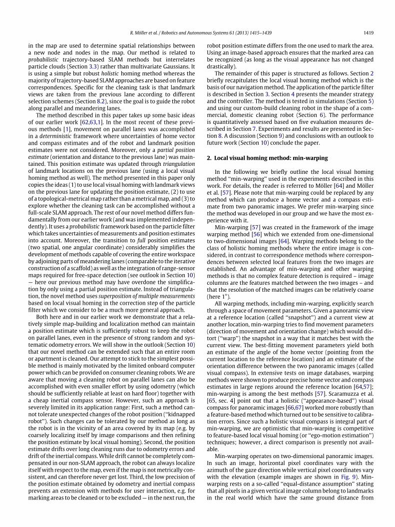
posdiff [m] For each map node, we determine the Eu-clidean distance between real and estimated position∥(x, y)−(xreal, yreal)∥ and average over allmapnodes.This measure is not determined in the robot experi-ments since it would require a mapping of the exter-nal coordinate system of the overhead tracker to therobot world coordinate system.
lanedev [m] For each map node, we search for the closestnode on the previous lane (minimal Euclidean dis-tance) according to its real position (known in thesimulation) and determine the absolute value of thedifference between the closest distance and the de-sired lane distance. The measure lanedev is the av-erage over all map nodes, beginning with the secondlane. In the robot experiments, each position esti-mate from the tracker is used.
fitdev [m] For each lane, we form a data set with the(xreal, yreal) positions of all map nodes (in the robotexperiments: tracker positions) and perform a prin-cipal component analysis (PCA) which fits a line withminimal perpendicular distance to all data points.The smallest eigenvalue is the average of the squaredperpendicular distances. Our measure fitdev is themean over all lanes of the square root of the smallesteigenvalue.
fitangdev [rad] We perform a PCA as for fitdev. We deter-mine the absolute value of the deviation of the an-gle of the fitted line βfit (obtained from the principaleigenvector) from the desired lane angle β byacos(| cos(βfit − β)|). This expression considers thatthe sign of the eigenvector is not determined. Themeasure fitangdev is the mean over all lanes. Inthe robot experiments, the desired lane angle β is theangle of the line fitted to the first lane.
angdiff [rad] This measure is only used in the analysis of therobot experiments. It determines the angular differ-ence (including the sign) between the line fit to eachlane and the line fit to the first lane. If βfit,0 is the an-gle of the line fit to the first lane and βfit the angleof the line fit to one of the other lanes, the measureangdiff is the average over sgn(cos(βfit − βfit, 0))asin(sin(βfit − βfit, 0)) over all lanes.
If runs with the same parameters are repeated multiple times, theaverage of a measure over all runs is given.
8. Experiments
In the following we describe the results of the experiments insimulations and with the real robot. In Section 8.1 we visualizethe effect of the artificial odometry errors which we introduced tomake the task ofmoving onparallel lanesmore demanding. Experi-ments in the simulatorwhere the visual homingmeasurements areobtained from a noise model are described in Section 8.2. Therewe also analyze the quality of different correction regimes usingdifferent numbers of homing-based correction steps. In the simu-lations described in Section 8.3, visual homing measurements areobtained from min-warping in a room with random wall textures.In this setup, the effect of delayed availability of visual homingmeasurements is studied. We also visualize the temporal develop-ment of the area covered by the particle cloud. Amore realistic sim-ulation setup where the walls of the virtual room are covered withphotos of our lab room is used in Section 8.4. The results of robotexperiments in this lab room are finally presented in Section 8.5.
8.1. Simulation: pure odometry
Fig. 10 gives a visual impression how the systematic speed er-rors and the speed noise affect the trajectory of the robot if no cor-rection but only prediction (without uncertainty, i.e. kodo = 0) isperformed. The top diagram shows the effect of a purely system-atic error which in a real robot may result from differences in thewheel diameters. Since the systematic speed errors of left and rightwheel have a different sign, the lanes are strongly curved and the
1428 R. Möller et al. / Robotics and Autonomous Systems 61 (2013) 1415–1439
Fig. 11. Simulation (with homing noise model). Evaluation measures posdiff, lanedev, fitdev, and fitangdev for varying odometry constant kodo and for threedifferent homing-based correction regimes, each measure averaged over 20 runs. The kodo axis is logarithmic.
resulting trajectory does not resemble the desired trajectory withparallel lanes. In the bottom diagram, the effect of a purely randomspeed error is visualized. While the desired shape of the trajectoryis still recognizable, the deviations from the desired trajectory canbe even larger than the lane length. In all simulation and robot ex-periments, systematic and random errors are introduced, with theparameters used to produce Fig. 10.
8.2. Simulation: homing noise model
We now introduce correction steps by range-sensor measure-ments (on the first lane) and by emulated visual homing measure-ments (on all subsequent lanes). Here we assume that the visualhoming procedure takes no time and the correction can be appliedimmediately; the effect of a delayed correction is studied in Sec-tion 8.3. Home vector and compass estimates are produced by thehoming noise model (Section 5.4).
We take the somewhat unusual approach to tune the odometryconstant kodo such that the quality of the trajectories is optimized.Fig. 11 shows the four evaluation measures posdiff, lanedev,fitdev, and fitangdev for varying odometry constant kodo andfor different homing-based correction regimes, eachmeasure aver-aged over 20 runs. The forward wheel speed (over ground) of therobot is 0.1 m/s, the turn wheel speed ±0.1 m/s. In each run, 14lanes with an inter-lane distance of 0.3 m are driven. The predic-tion step of the particle filter is performed every 0.1 s. On each lane,20 snapshots are captured in a distance of D = 0.1 m. On the firstlane, kodo = 0.001 is used in the prediction step, and the robot usesits range sensors to correct the position estimate (see Section 3.4).On all subsequent lanes, the correction step of the particle filter isbased on (emulated) visual homing data (superposition of all com-pass and home vector measurements, see Section 3.3.4). Duringturns and lane switches, only compass information relative to thelast snapshot on the previous lane is used in the correction. In the
figure, the odometry constant kodo used on lanes, during turns, andduring lane switches is varied between 0.0005 and 0.08.
As described in Section 3.3.4, the results of multiple local visualhoming computations are superimposed in the particle-filter up-date. For each update, the current view is compared to a landmarkview taken on the previous lane. On the one hand, the numberof updates should be as small as possible since the visual homingcomputations are the most time-consuming part of the particle-filter update. On the other hand, the number of landmark viewsand the location of the landmark views relative to the current lo-cation influence the quality of the robot’s trajectories: first, usingmultiple landmark views in different directions from the currentlocation constrains the likely position in different directions andthus improves the position estimate. Second, the closest landmarkview on the previous lane does not constrain the position estimatewith respect to the distance to the previous lane and would there-fore alone be insufficient for the cleaning task. Third, if the distancebetween current location and landmark location is large, the angu-lar uncertainty of the home vector angle leads to large positionaluncertainty and thus to less precise position estimates. Forth, con-sidering neighboring landmark views will only lead to small im-provements of the position estimate since, homevectors computedfrom these views both are likely to be correlated in their errors andconstrain the estimated location in similar directions.
In the following, three different homing-based correctionregimes are compared. Each regime uses either one, two, or threeviews on the previous lane for the correction step. These can be thespatially closest view on the previous lane, the forward viewwhichis approximately 45° ahead of the robot (3rd view forward fromthe closest view), and the backward view which is approximately45° behind the robot (3rd view backward from the closest view).It is clear that the closest view is optimal for correcting deviationsalong the lane. Appendix A shows that the ±45° angle is optimalto compensate deviations perpendicular to the lane. The three cor-rection regimes are
R. Möller et al. / Robotics and Autonomous Systems 61 (2013) 1415–1439 1429
Fig. 12. Simulation (with homing noise model). Typical runs for different values of kodo . Solid line: true robot position, cross marks: estimated robot position after eachcorrection step. All runs use the correction regime ‘‘superposition forward+backward+closest’’.
alternate forward/backward. Only a single landmark view isconsidered in each correction step, alternating between forwardand backward view.superposition forward+backward. Forward and backward view areused simultaneously in the correction step.superposition forward+backward+closest. Forward, backward, andclosest view are used simultaneously. This regime is visualized inFig. 4.
Each pair of views contributes both a home vector estimate anda compass estimate. At the lane end, a non-existing forward viewis replaced by a backward view; at the lane start, a non-existingbackward view is replaced by a forward view.
Fig. 11 shows that the regime ‘‘superposition forward+backward+closest’’ produces the best values in all four measures.In the following, we therefore use only this regime. The figurealso reveals that each of the four evaluation measures becomesminimal for different odometry constants; this will be explainedin the following.
With a small odometry constant kodo, the prediction step willproduce narrow particle clouds. Due to the large odometry errorused in our experiments, the robot position indicated by the sen-sor data will probably not lie inside the cloud, thus the correctionstep of the particle filter can only move the cloud center by a smallamount towards the real position. Consequently, the large odome-try error will lead to large deviations between the true and the es-timated robot positions (large values of posdiff). Moreover, theunder-compensated odometry error will result in large deviationsfrom the desired lane orientation (large values offitangdev). The
errors in the lane orientation also cause large deviations in the dis-tance between lanes from the desired lane distance (large values oflanedev). However, the lanes are relatively straight since the sen-sor data have only a small influence in the correction step (whichresults in small values of fitdev). This behavior is also visible inthe selected run in Fig. 12 (k = 0.0005) where especially the effectof the under-compensated odometry error is apparent.
With a large odometry constant kodo, the prediction step willproduce wide particle clouds. It is likely that several particles arelocated close to the robot position indicated by the sensor data,thus the correction step will shift the center of the cloud by a largeamount. Since the measurements obtained from the visual hom-ing method are noisy, this may lead to large jumps of the cloudcenter. This in turn will cause large deviations between true andestimated robot positions (large values of posdiff), large devia-tions from the desired lane distance (large values oflanedev), andawinded course on the lane (large values of fitdev). However, onaverage, the orientation of the lane is correct (relatively small val-ues of fitangdev). This behavior is also visible in the selected runin Fig. 12 (k = 0.08): large jumps can be observed in the positionestimate, but it still overall follows the true robot position (albeitwith large local deviations), and the lane orientations are approx-imately correct.
An intermediate value of kodo seems to be a good compromisewhich simultaneously satisfies all four measures. Fig. 12 (k =
0.006) shows a good correspondence between desired and truetrajectory and relatively straight lanes. In all following experi-ments, we therefore use kodo = 0.006.
1430 R. Möller et al. / Robotics and Autonomous Systems 61 (2013) 1415–1439
Fig. 13. Simulation (with min-warping and rendering, virtual room with randomwall texture). The true robot position of the 10 first runs (solid lines) and theestimated robot position of a single run (dashed line) are shown. No artificial timedelay between image capture and availability of homing results is introduced.(Note that trajectories are obtained by connecting snapshot positions. Thereforelane switches sometimes appear skewed since lanes do not necessarily end witha snapshot.)
8.3. Simulation: warping and random wall texture
In the simulation experiments in this section and in Section 8.4,image rendering and the true homing method (min-warping) areapplied (Section 5.5) rather than a homing noise model, thus theperformance is affected by the true errors made by the homingmethod. These include correlations in the errors if spatially adja-cent views are used (which are not reproducedby thehomingnoisemodel). The homing method and its parameters are described inSection 2. The camera heightwas 0.1mand the image size 360×60pixels with the horizon located at the lowest image row (thus thefloor is never visible). The virtual room’s randomly textured walls(Figs. 7 and 9) are high enough such that the rendered image neverincludes portions above any of the walls (so it is guaranteed thatthe visual homing procedure only relies on the random wall tex-ture and not on the borders between walls and floor or ceiling). Nocutoff filter was applied to the rendered image. The robot attemptsto capture 20 snapshots on each lane; however, if the distance tothe wall in front of the robot falls below 0.3 m (from the robot’sfront), the lane is terminated early. In total 14 lanes are driven.
Fig. 13 shows a superposition of 20 homing runs (obtainedwith different seeds provided to the random number generators).It is visible that the performance is qualitatively similar to thesimulation runs with homing noise model shown in Fig. 12(diagram for kodo = 0.006, which is also the value used here).We can conclude that the true rather than simulated errors of thehoming method do not noticeably affect the performance of thecleaning run. From the multiple runs overlaid in Fig. 13, the erroraccumulation of the lanes becomes apparent: later lanes showlarger deviations from the target lane than earlier ones. This is dueto the recursive nature of our correction schemewhere thepositioncorrection is based on snapshots collected on the previous lane.
Fig. 14 shows that the four performancemeasures only differ inthe range of one standard deviation between simulationwith hom-ing noisemodel (A) and simulationwith rendering and visual hom-ing method (B). In some measures (posdiff, fitangdev), truehoming leads to slightly larger deviations, while the performanceis slightly better in the other two measures (lanedev, fitdev).We think it can be safely concluded that the overall performanceis about the same.
To simulate the effect of a delayed correction (see Section 3.6),we introduced an artificial time delay of two prediction steps(0.2 s) in our simulation. A comparison of experiments B (no delay)and C (with delay) in Fig. 14 shows that the performance loss dueto the time delay is only small (about one standard deviation).
We observed that the particle cloud remains spatially confinedeven after several lanes. To give a visual impression of this behav-ior, we computed the covariancematrix of the position component(x, y) of all particles. In Fig. 15, the square root of the variances(main diagonal elements of the covariance matrix) and the squareroot of the absolute cross-covariance entry (with the sign reintro-duced afterwards) are visualized. In the top diagram it can be seenthat the variances rise when the lane is changed (13 peaks) but arereduced again over the lane. During lane switches, the cloudmainlyelongates perpendicularly to the lanes (in x-direction) since onlythe compass estimate is used for the updatewhich can only confinethe cloud in the direction of the lanes. The segment shown in thebottom diagram shows that the variances increase over timewhileonly prediction steps are applied, and are reduced again after a cor-rection step based on visual homing has been inserted. Overall, thecloud remains almost circular in shape: compared to the variances,the covariance is small, and the variances are similar to each other.
8.4. Simulation: warping and wall photos
We now make the simulation even more realistic by switchingto a virtual room where the walls are covered with photos of thewalls in our lab room (note that we do not model the depth struc-ture of objects in the room).While low frequencies are emphasizedwhen the random wall texture is used (Section 5.5), higher im-age frequencies can be obtained for the wall photos. Since warpingmethods are known to work slightly better for moderately low-pass filtered images [64,57], we apply a Gaussian filter with a rel-ative cutoff frequency of 0.3 (note that the filter is applied to thepanoramic image here whereas it was applied to the original cam-era image in our previous publications). The effect of this low-passfilter is visualized in Fig. 9. The camera height was 0.1 m and theimage size 360 × 30 pixels with the horizon located at the bottomrow (thus the floor is never visible). Even though the image heightwas reduced to 30 pixels (compared to 60 in the roomwith randomwall texture), small portions of the ceiling can be visible from somepositions. Since no photo of the ceiling is available, a middle graytone was used for all ceiling pixels. The homing results are delayedartificially by 2 prediction steps.
Fig. 16 presents the results for two runs with different laneorientations. In these runs, neither the number of snapshots perlane nor the number of lanes was specified; instead, a lane ends ifthe distance between robot front andwalls drops below 0.3m, andthe entire run ends if not enough free space remains to add anotherlane (note that the walls are not shown). In the top diagram, thesimulated robot drives long lanes of almost 8 m length (probablya rare case in apartments). Here the accumulating errors becomeobvious after about 8 lanes. Even though the later lanes are curved,there is still no crossing-over between lanes or larger gaps betweenthe lanes, thus the cleaning task can still be performed efficiently.In the bottom diagram, the simulated robot drives a large number(26) of shorter lanes (but still of almost 5 m length). Here largerdeviations from the target lanes also occur after about 8 lanes.Again, the effect on the cleaning performance is small.
8.5. Robot experiments
The robot experiments were performed in our main lab room(the same room from which the wall photos in the simulation ex-periments in Section 8.4 were taken, see Fig. 8). The opaque cur-tains in front of the windows were closed such that the conditionsof illumination were constant. We used the tracking system de-scribed in Section 6.2 to determine the robot’s position in the room.Along the first lane, the robot follows a low fence which is not vis-ible in the robot’s camera image.
R. Möller et al. / Robotics and Autonomous Systems 61 (2013) 1415–1439 1431
Fig. 14. Mean and standard deviation over 20 runs for the four different evaluation measures. A: Simulation with homing noise model. B: Simulation with min-warping andrendering, virtual room with random wall texture. It is assumed that the correction step can be performed without delay. C: As in B, but the correction step is delayed by0.2 sec (2 additional prediction steps are executed before the correction is applied retroactively).
Fig. 15. Visualization of the covariance matrix of the (x, y) components of theparticle cloud for a single run (kodo = 0.006, room with random wall texture). Top:Time course of the entire run (14 lanes), with cubic spline interpolation. Bottom:Segment from particle filter step 1500 to 2100, no interpolation.
The robot is controlled by the same software as used for the sim-ulations, except that sensor data come from the robot and motorcommands are passed to the robot. The control software runs ona laptop and communicates via wireless LAN with servers runningon the onboard PC of the robot. One of the servers continuouslycaptures camera images and assigns time stamps to each. If an im-age is requested by the control software at one point in time, theimage with the closest time stamp is provided by the server. Thesame server also modifies the exposure time of the camera suchthat the mean intensity of the image is approximately kept con-stant. Histogram equalization and a low-pass filter (binomial filter,kernel size 11) are applied. Images have the size 360×48 with thehorizon located at the bottom row; the elevation covered is 38°(thus the resolution in horizontal and vertical directions differs).The lens top is mounted approximately 9.6 cm above ground. Toavoid systematic errors introduced by the small delay between thecommands for the left and the right motor, motor commands aresent in random order to the two separate controller boards. A sin-gle loop in the main control loop of the robot has the same lengthas in the simulations (0.1 s); if a loop is completed in shorter time,an appropriate delay is inserted.
Fig. 16. Simulation (with min-warping and rendering, virtual room with wallphotos). Real position (solid line) and estimated position (dashed line) for twoselected runs are shown. Both runs start at (0.3 m, 0.3 m). Lanes are terminated ifthe range sensors indicate that the frontal distance to a wall dropped below 0.3 m(from the robot center). If there is not enough space to start another lane, the runstops. The first lane is driven along the bottom and the left wall, respectively. Thewalls are not shown. (See also note in Fig. 13.)
The speed on lanes was 0.15 m/s (slightly faster than in thesimulation), and 0.1 m/s during turns and lane switches. Althoughthe image with the closest time stamp to the time of request isprovided, the image can be old (especially if the exposure timeis long). To exclude this possible error source, especially after
1432 R. Möller et al. / Robotics and Autonomous Systems 61 (2013) 1415–1439
rotations, we introduced a delay of 0.5 s before the robot startsto move on a new lane. The delayed correction scheme for theparticle filter (see Section 3.6) is used, here with the true delayscaused by the homing computation. The homing computation isspread to 3 threads which are likely to run on separate cores ofour quad-core control laptop. Since we observed that the homevector errors are larger than in the simulated runs in the roomwiththe wall photos (which is probably due to occlusions, violations ofthe equal-distance assumption of min-warping, and reflections, allof which are not considered in the simulations), we increased thestandard deviation assumed in the particle filter to σH = 0.5 rad(see Section 3.3.2). The compass estimates are approximately asprecise as in the simulation. Since the reduced quality of the homevector estimates also causes larger jumps in the position estimate,we increased the distance to the sliding target point on the lane toL = 1.0 m (see Section 4.2) to iron these jumps out.
Fig. 17 (top row) shows the target trajectories of the robot ex-periments in our laboratory room. For each of the two trajectories,we performed five runswith systematic speed errors ηl = −0.025,ηr = 0.025 (called ‘‘left’’, since, if uncorrected, the robot wouldturn to the left), and another five runs with ηl = 0.025, ηr =
−0.025 (‘‘right’’). The speed noise was ϵ = 0.2 in both cases.Fig. 17 (bottom rows) shows the robot trajectories captured by
the overhead tracking system. It is visible that the large systematicerror (compare with the uncorrected trajectory in Fig. 10, top,which is also observed in robot experiments without correction) isalmost compensated; only a much smaller tendency of orientationchange in the direction of the systematic error (‘‘left’’, ‘‘right’’)remains. For both target trajectories, the lanes are approximatelyparallel, but there are deviations from the perfect lane distancewhich would cause small areas between the lanes to be cleanedtwice or to be left out. No crossover of adjacent trajectories occurs.The overlay of the five trajectories for each experiment shows thatthe behavior is reproducible.
Table 1 (top) lists the averages over five runs each for themeasures laneDev, fitDev, fitAngDev, and angDiff for eachof the four experimental conditions. Whenwe compare the resultswith those obtained from simulations (Fig. 14), we see thatlaneDev, the deviation from the desired inter-lane distance, isin the range between about 3 and 5 cm and thus higher thanthe approximately 2 cm in the simulations. The measure fitDev,which describes deviations from the straight lane, is only slightlyhigher than in the simulations (1–2 cm, compared to about 1 cmin the simulations). Also the range for the measure fitAngDev iscomparable to that obtained in the simulations (somewhat smallerif averaged over the two 7 × 40 experiments, somewhat larger ifaveraged over the two 14×18 experiments). Overall, the behavioris only slightly worse than in the simulations. We ascribe thereduced quality mostly to the larger deviations in the home vectorwhich we observed in the real robot experiments. We alreadymentionedpossible reasons for this above, all of themeffectswhichwere not considered in the simulations (occlusions, violations ofthe equal-distance assumption, reflections).
The measure angDiff was only computed for the robot runs.As the last column of Table 1 (top) shows, there is a tendency ofthe lane orientation to follow the direction of the systematic error,an effect that was also apparent in Fig. 17 (bottom rows). This maymostly be due to error accumulation over the lanes caused by ourupdate regimewhich only refers to snapshots on the previous lane.
The method described in this work uses a probabilistic frame-work based on the particle filter which produces a full posi-tion estimate, whereas the precursor to our method describedby Gerstmayr-Hillen et al. [1] used a deterministic frameworkbased on triangulation which only produced a partial position es-timate. The robot experiments for both studies were performedunder comparable conditions (same robot except for a different
panoramic optic, same room, comparable number and length oflanes, same inter-lane distance, same local visual homing method,same systematic odometry errors). The only differences are thatin [1] no random odometry errors were used and that the robotspeed on the lanes was only 0.075 m/s. The robot position dataobtained from the overhead tracking system for the experimentspresented in [1] were available. We analyzed these data using theevaluation measures suggested in this paper; see Table 1 (bot-tom). If we compare the total averages given at the bottom row ofeach table, we see that a noticeable difference occurs for the mea-sure fitDev: The novel method presented in this paper producesstraighter lanes. Even though the lanes produced by the methoddescribed in [1] are more curved, this has no effect on the measurelaneDev which expresses deviations from the desired inter-lanedistance and directly affects cleaning efficiency. This can probablybe explained by the fact that the method by Gerstmayr-Hillen etal. [1] propagates deviations from one lane to the next such thatcurves driven on one lane are often followed on the next. Althoughalready the older method yields a surprisingly good cleaning per-formance on a rectangular area, we think that our novel methodsimplifies the extension to multiple meander parts, as will be dis-cussed below.
9. Discussion
In this work we introduced a novel method for the lanecontrol of cleaning robots. It differs in several aspects from thetypical approaches to navigation problemswhich are characterizedby the use of geometrical maps of landmarks corresponding toimage features, correspondence methods for the matching ofvisual features, and full-scale SLAM mechanisms. Our approach,in contrast, builds topo-metric maps, uses panoramic views aslandmarks, compares entire images by a holistic visual homingmethod, and only uses a simple particle filter without continuousupdate of all estimates. Our main motivation for choosing thisdirection is parsimony: easy-to-construct graph maps wherenodes are annotated with low-resolution images, an extensionof the map by adding nodes without later refining their positionestimates, and a particle filter instead of full-scale SLAM promiseto be less memory- and time-demanding and may, in our opinion,be sufficient for the cleaning task at hand. This also fits well withthe limited computational power which is usually available onhousehold cleaning robots.
Our goalwas to demonstrate that themethod is capable ofmov-ing a cleaning robot on parallel lanes in order to efficiently clean arectangular area. Our extensive simulations and robot experimentshave shown that the method produces parallel lanes with approx-imately constant inter-lane distance even if the robot’s odometryis heavily perturbed by large systematic and random errors (whichwere artificially introduced since the robot platform exhibitsmuchsmaller natural errors). The successful application of our methodshows that the precision of the simple visual homing method atits core (min-warping) is sufficient for this task, and that the con-cept of using views (and particle clouds) as landmarks (rather thanexternal features) produces reliable robot position estimates.
While the cleaning quality achieved in the robot runs is compa-rable to the results of our earlier, deterministicmethodwith partialposition estimates [63,1] (albeit with straighter lanes in our novelmethod), a full position estimate makes it much easier to extendthe method such that complex workspaces can be cleaned by ad-joining multiple rectangular areas. Estimates of positions obtainedat the border of one part of meandering lanes can be used to esti-mate the position of the first lane of an adjacent part by the samemeans as done between lanes within the same part (see Section 10and Fig. 18). Moreover, a full position estimate is required to buildrange-sensor maps which are necessary for the detection of un-cleaned areas.
R. Möller et al. / Robotics and Autonomous Systems 61 (2013) 1415–1439 1433
Fig. 17. Top row: Approximate location of the target trajectories for the robot experiments in our laboratory room. The trajectories start at the position marked with thecircle and end at the arrow head. The scale bars at the bottom left are 1m long. The room contains desks, office chairs (visible as pentagons), and a robot arm setup (H-shapedstructure on the left); see also Fig. 8. Top left: Target trajectory with 7 lanes and 40 snapshots per lane (‘‘7× 40’’). Top right: Target trajectory with 14 lanes and 18 snapshotsper lane (‘‘14 × 18’’). Bottom rows: Robot trajectories captured by the overhead tracking system for the two target trajectories and for the two types of systematic speederrors specified in the text (middle row: ‘‘left’’, bottom row: ‘‘right’’). All 5 trajectories of each experiment are plotted. The first trajectory is shown with thick lines.
Table 1Results of robot experiments: average of themeasureslaneDev,fitDev,fitAngDev, andangDiff over five runs each, and average overall runs (except for angDiff). Top: Results of the experiments with the method presented in this paper (probabilistic, particle filter, fullposition estimate). Bottom: Results of experiments by Gerstmayr-Hillen et al. [1] (deterministic, triangulation, partial position estimate).
8 × 41 left 0.0352 0.0278 0.0247 −0.01368 × 41 right 0.0391 0.0321 0.0299 −0.026515 × 21 left 0.0353 0.0263 0.0635 0.058515 × 21 right 0.0443 0.0276 0.0447 −0.0070
Average 0.0384 0.0284 0.0407
1434 R. Möller et al. / Robotics and Autonomous Systems 61 (2013) 1415–1439
Fig. 18. Preliminary results for a more complex cleaning strategy built on the method for meandering trajectories presented in this paper. Left: Simulation. Obstacles (walls,furniture) are taken from a realistic model of an existing apartment. The dot (top center) marks the start point. Only the cleaning lanes are shown, not the movementsbetween the meander parts. Right: Robot experiment in an office room. Robot trajectories are obtained from an overhead tracker. Shaded regions show the area covered bythe suction port (darker color: multiple coverage). The double arrows mark start and stop position of the robot.
Although the method contains a number of parameters (as-sumedmeasurement noise in the particle filter, scale factor lists inmin-warping etc.), only one of them has to be chosen carefully inorder to guarantee good cleaning performance. This parameter isthe odometry constant kodo which affects the growth of the particlecloud in the odometry-based prediction step of the particle filter.We selected a valuewhich is optimal for the large artificial system-atic and randomodometry noise. In further robot experiments (notshown in this paper) where the odometry was only affected by themuch smaller natural odometry errors, we found that the chosenvalue is also suitable. However, it may be possible to achieve evenbetter results by adjusting kodo for this situation. In the transitionfrom simulations to robot experiments we noticed that the perfor-mance of min-warping degrades to some extent. This is due to oc-clusions (image parts appearing or disappearing between snapshotand current view), violations of the equal-distance assumption onwhich min-warping rests (Section 2), and reflections and lighting(which are not reproduced in our simplified simulation).6 Weman-aged, however, to compensate for this by increasing the home vec-tor noise assumed in the particle filter and by stronger averagingover jumps in the position estimate by means of a larger distanceto the sliding target point.
10. Conclusions and future work
The experiments demonstrate that our non-mainstream nav-igation method is capable of guiding a cleaning robot along me-andering lanes with only small deviations from the optimal lanedistance required for efficient cleaning, even in the presence oflarge odometry errors. Cleaning of rectangular areas on mean-dering lanes is the building block for cleaning strategies coveringthe entire reachable area of a room or apartment; we outline thepresent state of our work and present preliminary results in Sec-tion 10.1. On such long runs in complex environments, the loop-closure problem becomes relevant, at least to ensure that all areasare cleaned and no area is cleaned multiple times; we sketch theapproach we want to take in Section 10.2. Although we are not
6 Both simulations and robot experiments are affected by anisotropic distribu-tions of landmarks (especially if the robot is close to a homogeneous wall such thatall other landmarks are clustered on one side of the panoramic image) which makeit difficult for min-warping to discriminate between effects of translation and rota-tion of the robot.
convinced that a full-scale SLAM approach is actually required tosolve the cleaning task,we provide preliminary results on the qual-ity of position estimates of an alternative trajectory-based SLAMmethod in Section 10.3. The meander pattern used in our methodis typical also for commercial domestic cleaning robots. However,out method could also be used together with other basic cleaningpatterns. We discuss possible alternatives and explore the aspectsof complete coverage and cleaning efficiency in Section 10.4. Im-provements and alternatives to our local visual homingmethod arediscussed in Section 10.5.
10.1. Extension to multi-part cleaning strategy
We are currently working on an extension to more complexcleaning strategies where a room or apartment is covered byadjoining regions of parallel meandering lanes (as described inthis paper). These regions (in the following called ‘‘parts’’) arenot necessarily rectangular as in the experiments performed here,but each lane can be as long as or shorter than the previous lane(if obstacles are encountered); it should not extend beyond theprevious lane to keep the distance to the landmark nodes small. Ifno more lanes can be added to a part, a planner consults the topo-metric map (containing nodes characterized by landmark viewsand by their position estimates in the form of a particle cloud) andan obstacle map (containing range-sensor measurements relativeto eachmapnode) and suggestswhere the first lane of the next partcan be added. The starting point of the first lane is always located ata given distance (usually corresponding to the width of the suctionport) from an existing map node. Planning considers the lengthof the first lane and the distance from the current location to thestarting point of the first lane. The first lane of the next part isalways chosen such that it runs adjacent to an existing part, oftenwith lanes running perpendicular to those of the predecessor part,such that landmark views at the border of the previous part can beused for the position correction step of the particle filter. A shortestpath is planned from the current location to the starting point ofthe first lane, and the path is followedwhile continuously updatingthe position estimate by referring to nearby landmark views. Therobot then switches to the meandering mode described in thispaper until another part needs to be added. In thisway, amulti-partmap is constructed which in the end covers the entire reachablearea. The robot can then use the map to return to its starting point.
Fig. 18 (left) shows a result from a computer simulation (basedon the homing noise model, see Section 5.4) in a realistic floor
R. Möller et al. / Robotics and Autonomous Systems 61 (2013) 1415–1439 1435
plan of an apartment containing walls and furniture at robotheight as obstacles. Only lanes are visualized, not the transitionalmovements between parts. It is visible that the entire reachablearea is covered (except for regions close to obstacles for which anadditional strategy like wall-following needs to be added). Fig. 18(right) presents the results of a robot experiment in an office room.The figure shows the robot’s entire trajectory (cleaning lanes andtransitional movements between parts) obtained by an overheadtracking system. The shaded areas are the regions covered by therobot’s suction port, darker colors indicate multiple coverage. Forthis preliminary experiment we did not take measurements of theobstacle locations. The room contained office chairs, book cases,a writing desk, and a conference table. The latter was fenced off(region in the upper left) since the tracking system would lose therobot if itmoves underneath the table. At the bottom left it is visiblehow the robot circumnavigates a small cabinet which was placedthere to make the task more demanding. In a small region at thebottom left the robot temporarily leaves the range of the overheadtracking system. After cleaning the reachable area, the robot usesthemap to return to the starting point (starting point and end pointare marked by double arrows).
10.2. Loop closure
Long multi-part runs as described above will of course empha-size the loop-closure problem. The robot may return to an alreadycleaned region on another path. Attempting to detect this situationbased only on position estimatesmay fail due to the drift of the po-sition estimate. The robot would then clean the area a second time,or, even worse, may stop cleaning before the gap is closed since itassumes that the cleaned region has already been reached. Again,we attempt to stick to our parsimonious approach by solving thisproblem through a simple visual loop-closure detection [61] ratherthan an extension to a full-scale SLAM approach. If a loop closure isdetected, local visual homing could be used to determine the posi-tion error. The map could then be corrected such that this error isreduced. We plan to test whether it is sufficient to only correct theposition and orientation of entire parts rather than those of eachmap node. By extending themethod by loop-closure detection andmap correction we will of course approach full-scale SLAM.
10.3. SLAM
Even though our method in its present form cannot preventposition drift, full-scale SLAMmay not be required for the cleaningtask. Using the topo-metric map, even if it is not metricallyconsistent, the robot is able to localize itself and can never get lost,as long as it is located in the vicinity of the region covered by themap. Considering that a tree of adjacent and linked meander partsis constructed, it will always be possible for the robot to plan apath to an arbitrary node in the map (e.g. the home position) and –an unchanged environment presumed – to approach this locationwhile continuously updating the position estimate through visualhoming. Even if the robot is kidnapped, it could localize itself byfirst comparing the current image to all images stored in the mapand then subsequently updating its position estimate through localvisual homing.
We will, nevertheless, test trajectory-based SLAM approaches(see Section 1.2.2) based on our topo-metric maps for comparisonwith our method. In the following we present preliminary resultson the quality of the position estimates and on the computationaleffort for both approaches. In the experiments, the robot wascontrolled by the particle-filter method described in this paper,and the trajectory-based SLAM method was running in paralleland computing its own position estimates based on the sameodometry and visual information. The estimated robot positions of
each method were compared to the true robot positions obtainedfrom the overhead tracking system. We optimally aligned therobot’s world coordinate system (which coincides with the robot’sstart pose) and the tracker coordinate system using the Kabschalgorithm7 [71,72]. We analyze the mean deviation between thealigned estimated and real positions.
We implemented a full trajectory-based SLAMmethodbased onan exactly sparse extended information filter (ESEIF) [40]. We addan additional delayed state whenever a node is inserted into ourmap. The relations between the poses are stored as an informationmatrix, which is the inverse of the covariance matrix, and aninformation vector. In our special case, where links between twoposes are only inserted for pairs used for homing, the matrix isvery sparse. This allows for a compact storage of the data, evenfor a large number of poses. The covariance matrix, in contrast,would be filled completely. Esteban et al. [45] extract the relativepose between two nodes from the essential matrix obtained byextracting SIFT-features from the corresponding images. In ourcase,weuse thewarping results (homevector and compass) for thecorrection step. In the information-filter approach, the most time-consuming operations are required to compute the metric posesby solving a system of linear equations, as the measurement andmotion equations have to be linearized at the current pose for eachmodification step. Currentlywe use a sparse Cholesky factorizationprovided by the ‘Eigen’ matrix library for this task, although othermore efficient methods may be available.
The experimental setupwas similar to the 14×18 experimentsdescribed in Section 8.5. Again, five runs each were performedwith systematic odometry errors in both directions. To give bothmethods the best chances, we used an improved version of min-warping.8 On the first lane we use method (2) from Section 3.4since the range-sensor update used by method (3) is not imple-mented in the SLAMmethod.
Using the particle-filter method described here, the mean overall 10 runs of the mean deviations between estimated and trueposition was 0.0478 ± 0.0088 m. The trajectory-SLAM methodperformed somewhat better with 0.0317 ± 0.0072 m. The com-putational effort of the particle-filter method is dominated by thecorrection step based on visual homing (see Section 3.3). A cor-rection based on home-vector and compass estimate for a singleimage pair takes about 3 ms on an Atom N2600 CPU (a typicalprocessor for embedded systems which might be used in a com-mercial cleaning robot). This effort stays constant when the mapgrows since the position estimate of a node is never changed afterit was inserted. The computational effort of the trajectory-SLAMmethod grows linearly with the number of map nodes. Aroundthe end of the single meander part, the map contains about 200nodes. The effort is dominated by the computation of the met-ric poses (see above) which takes about 12 ms for each update.The rest of the SLAM method is surprisingly fast (about 2 ms at200 nodes). The correction step of the SLAM method is performedboth for odometry and for homing updates. Each homing updatestep of the particle filter method considers three image pairs. Sinceodometry prediction and homing correction are performed in aratio of about 6:1, the SLAM update requires 7 × 12 = 84 ms,whereas in the same time the particle filter update only requires1× 3× 3 = 9 ms. Compared to the effort for a three min-warping
7 The translation is computed by aligning the centroids of both data sets, therotation is determined from the SVD of the covariance of the resulting data, andfinally the scaling is obtained from a least-square fit.8 120 steps for the two search parameters (72 before), double matching
mechanism where the results of two matches with exchanged input images aresuperimposed (single matching before), larger vertical opening angle of 75° (38°before), exact magnification (linear approximation before).
1436 R. Möller et al. / Robotics and Autonomous Systems 61 (2013) 1415–1439
computations (3 × 240 ms for our fastest SSE-based implementa-tion on the Atom CPU), the effort for the correction step of the par-ticle filter is negligible and the effort for the SLAMmethod only getsinto the same range as min-warping for large maps (1700 nodes,which would be reached for an entire apartment).
Unfortunately, in our opinion, the results of this preliminarycomparison of the two approaches are inconclusive. The SLAMmethod does not dramatically improve the precision of the posi-tion estimate, at least for a single meander part, and even thoughthe particle-filter method will be noticeably faster for large maps,the computational effort for both methods is presently dominatedby the effort for min-warping. The computational advantage of theparticle-filter methodwould only become relevant if min-warpingcould be replaced by a much faster visual homing method. More-over, both methods have room for improvement. The correctionstepwould bemuch faster if the particle filterwould be replaced bya Kalman filter — in the particle filter, the number of computationsdepends quadratically on the number of particles (each particle inthe current cloud is related to each particle in the landmark cloud).We are sure that also the time-consuming pose computation of theSLAM approach can be accelerated by using amore efficientmatrixsolver.
Please note, however, that these results were obtained for onlya single part of meandering lanes. We will explore how the twomethods perform on multi-part trajectories. For this we have toadd a loop-closure detection method (for both approaches) and,for the particle-filter approach, a separate method to correct theposition estimates when a loop closure is detected. Moreover,we can presently not say how the cleaning performance wouldimprove if the trajectory-SLAM method would actually be used tocontrol the robot’smovements (extensive changes are necessary toadapt the code of our cleaningmethod such that all data structures– obstacles, target lanes etc. – change when position estimatesare updated by the trajectory-SLAM method; similar changes arerequired in the particle-filter approach if position estimates arecorrected when a loop closure is detected).
10.4. Cleaning patterns and cleaning strategies
The basic cleaning pattern of meandering lanes is shared byall second-generation domestic cleaning robots available on theconsumer market we are aware of (see Section 1.1.1), and wealso decided to use this pattern. However, our navigation method(‘‘local visual homing and particle clouds as landmarks’’) wouldalso allow alternative movement patterns. The only prerequisiteis that a sufficiently large number of landmark views has to beavailable in the vicinity of the robot’s location in order to correctthe position estimate. The landmark views should be located suchthat they impose constraints in different directions on the positionestimate (see Section 8.2). In themeander pattern, this prerequisiteis clearly fulfilled for all lanes except the very first one. It wouldalso be fulfilled if the robot cleans a small region by spiral orzigzag movements and then repeats this process in the immediatevicinity of a cleaned area. Our navigation method is less suitablefor patterns where the robot first surrounds a region by movingalong obstacles (wall following). In this case, only a small numberof previous and nearby landmark views would be available for theposition correction, and these views would constrain the positionestimate only in the same directions, which we assume wouldlead to a relatively large drift of the position estimate over longerdistances.9
9 In fact we observed this effect in the experiments where we used method (2)described in Section 3.4 to drive the first lane. We therefore restrict the length ofthe first lane if method (2) is used. Method (2) is only used in the experiments inSection 10.3.
We think that the multi-part strategy outlined in Section 10.1is able to completely cover the reachable area, at least if the rangesensors reliably reveal free space. As long as there is an uncleanedarea adjacent to a cleaned part in the map, the robot will attacha new part at this location. We are currently working on someextensions for special cases like tight passages which prevent ameandering movement. However, we cannot present a proof thatcomplete coverage is guaranteed.
Another question is whether the cleaning strategy efficientlycovers the reachable area, e.g. expressed by the ratio of requiredpath length to reachable area. We think that some basic cleaningpatterns (meander, spiral, but not zigzag) achieve a good efficiency(small ratio) within a single part. However, the cleaning strategyneeds to combine these basic patterns such that the entire reach-able area is cleaned, in our method by adding a new meander re-gion adjacent to regions already covered and captured in the map.This requires transition movements to reach the next area to becovered by the basic pattern (as visible in Fig. 18, right). It will beunavoidable to cross cleaned regions in this process which impairsthe efficiency. It is the task of the planner to use the obstacle infor-mation available at the present state in order to select the next re-gion such that the overall transitionmovementswill beminimized.However, in our case, the obstacle information is limited for tworeasons: First, the range sensors used onour robot only have a shortrange (about 1 m), and second, we assume that fresh topo-metricand obstacle maps are constructed in each cleaning run. Even if wewould use maps obtained from previous runs for planning an opti-mal cleaning trajectory, changes in the obstacles (moved chairs, abag on the floor, open and closed doors etc.) would prevent us fromexecuting this optimal strategy. We therefore think that investingeffort in the development of an optimal coverage planner wouldbe wasted. Instead, we will develop heuristics for the selection ofthe next part during the cleaning run. We will test these exper-imentally in real apartments and compare the resulting cleaningefficiency.
10.5. Local visual homing method
The performance of our navigationmethod depends strongly onthe quality of the home vector and compass estimates providedby the local visual homing method, currently min-warping. Wewill therefore in parallel work on improvements of min-warpingor related holistic methods. One important issue for a real-worldapplication of the method is illumination invariance. The exper-iments in our lab were performed under constant conditions ofillumination (closed curtains). We nevertheless employed a par-tially illumination-invariant distance measure (Eq. (2)) in the ex-periments presented here, since the gain control mechanism of thecamera and the histogram equalization applied to the camera im-ages (Section 6.1) cause intensity changes as well. More advancedmechanisms from the plethora of distance measures that havebeen suggested in the literature (e.g. [73]) can be applied. Alterna-tively, min-warping could be replaced entirely by a method whichextracts home vector and compass from feature correspondences.Fast binary descriptors such as BRIEF [74] or ORB [75] should besufficiently fast even for an onboard implementation with limitedcomputational power (application to navigation: [76]).
In its present form, our method ignores the correlations be-tween multiple measurements of home vector angle and visualcompass when the same current view is paired with several snap-shots on the previous lane. It may be beneficial to model thesecorrelations using covariance matrices and consider them in theparticle-filter update. In addition, mechanisms similar to inno-vation gates could be used to exclude measurements from theparticle-filter update which largely deviate from their expectedvalues.
R. Möller et al. / Robotics and Autonomous Systems 61 (2013) 1415–1439 1437
Fig. A.19. Sketch illustrating the computation of the bearing angle β which isoptimal for reducing the position uncertainty perpendicular to the lane. Twosubsequent lanes (index i and i + 1) with a distance d are shown as solid lines.The reference (snapshot) location is S, the current location is C. The angle α is thestandard deviation of the angular error of the home vector.
It is apparent that our method is affected by error propagationfrom lane to lane since only snapshots on the previous lane areused to update the position estimate on the current lane. Here wecould employmore advanced update schemeswhere snapshots onthe next-to-last or even earlier lanes or earlier snapshots on thesame lane are considered. Increasing the spatial distance betweensnapshot and current view may also improve the performance ofmin-warping since it is known that the home vector estimate ismore strongly affected by image noise the smaller this distancebecomes [56]. This may especially be helpful if the distance to thesurrounding landmarks is large (in the center of a large room) com-pared to the distance between the snapshot and current location.
Acknowledgments
We are grateful to Tim Köhler and Frank Röben for their valu-able contributions in the design of the robot and the develop-ment of its basic software suite. We thank our technician KlausKulitza who was responsible for part of the mechanical construc-tion and developed most of the robot’s electronics, and the teamof the university’s mechanics workshops. Our students AndreasStöckel and Thomas Schöpping designed parts of the softwareof the tracking system used in this study, many thanks to themas well. The simulation uses a von-Mises generator kindly pro-vided by Alexandre Campo (http://www.sourceware.org/ml/gsl-discuss/2006-q1/msg00033.html).Funding
This project was supported by Deutsche Forschungsgemein-schaft (DFG), grants MO 1037/2-1 and MO 1037/2-2 to RalfMöller and Excellence Cluster ‘‘Cognitive Interaction Technologies’’EXC277.
Appendix A. Best bearing angle
For a home vector correction step in the particle filter (seeSection 3.3.2) wewant to select snapshot locations on the previouslane for which the method achieves the smallest uncertaintyafter the home vector correction step (I) along the lane and (II)perpendicular to the lane. For (I), we just select the closest snapshotlocation on the previous lane; this obviously facilitates a reductionof the uncertainty of the position estimate along the lane, but noreduction of the uncertainty perpendicular to the lane. For (II),we now determine the optimal angle between the lane and thedirection to the snapshot location which is used in the update.
Wederive this optimal angle froma simple geometrical analysisbased on Fig. A.19. The figure shows two subsequent parallel laneswith an inter-lane distance called d. The agent is currently movingalong lane i + 1 and has captured the current image at location
C. It selects a snapshot location S on the previous lane i for thehome vector correction. The distance a is the distance from S to theclosest point to C on lane i. We assume that the error of the homevector angle measurement follows a distribution with standarddeviation α. If the error assumes the positive or negative value ofthe standard deviation, the position estimate forCwill then deviateby y1 and y2, respectively, on average by y = (y1 + y2)/2, inperpendicular direction to the lane i + 1.
There are two conflicting influences on the perpendicular de-viation y. On the one hand, the smaller the angle β = atan(d/a)becomes, the better can a perpendicular deviation be corrected(whereas in the other extreme β = 90°, no correction is possiblein perpendicular direction, see condition (I) above). On the otherhand, the smaller β becomes, the larger is the distance between Sand C. The same angular deviationαwill therefore result in a largerspatial deviation. We assume that there is an optimal angle β andtherefore treat the problem as optimization problem. The perpen-dicular deviation y can be written as
y =y1 + y2
2=
a2
tan
atan
da
+ α
− tan
atan
da
− α
,
which, after some manipulations, turns into
y =a(d2 + a2) tanαa2 − d2 tan2 α
≈
d2
a+ a
α. (A.1)
For small error angle α we approximated tanα ≈ α and tan2 α ≈
0. The optimum has to fulfill ∂y/∂a = 0 which gives d2 = a2 andthus a = ±d and β = ±45°. Thus the optimal direction for re-ducing the uncertainty in perpendicular direction is approximately45° in forward and in backward direction (it is clear that this willto some extent also reduce the uncertainty along the lane).
References
[1] L. Gerstmayr-Hillen, F. Röben, M. Krzykawski, S. Kreft, D. Venjakob, R. Möller,Dense topological maps and partial pose estimation for visual control of anautonomous cleaning robot, Robotics and Autonomous Systems 61 (2013)497–516.
[2] T. Palleja, M. Tresanchez, M. Teixido, J. Palacín, Modeling floor-cleaningcoverage performances of some domestic mobile robots in a reduced scenario,Robotics and Autonomous Systems 58 (2010) 37–45.
[3] E. Prassler, K. Kosuge, Domestic robotics, in: B. Siciliano, O. Khatib (Eds.),Springer Handbook of Robotics, Springer, 2008, pp. 1253–1281.
[4] H. Choset, Coverage for robotics—a survey of recent results., Annals ofMathematics and Artificial Intelligence 31 (2001) 113–126.
[6] Y. Liu, X. Lin, S. Zhu, Combined coverage path planning for autonomouscleaning robots in unstructured environments, in: Proceedings of the IEEEWorld Congress on Intelligent Control and Automation, WCICA, 2008,pp. 8271–8276.
[7] C. Luo, S.J. Yang, A bioinspired neural network for real-time concurrent mapbuilding and complete coverage robot navigation in unknown environments,IEEE Transactions on Neural Networks 19 (2008) 1279–1298.
[8] Y.H. Choi, T.K. Lee, S. Baek, S.Y. Oh, Online complete coverage path planningfor mobile robots based on linked spiral paths using constrained inversedistance transform, in: Proceedings of the IEEE/RSJ International Conferenceon Intelligent Robots and Systems, IROS, IEEE, 2009, pp. 5788–5793.
[9] S. Thrun, W. Burgard, D. Fox, Probabilistic Robotics, MIT Press, 2005.[10] R. Siegwart, I.R. Nourbakhsh, Introduction to Autonomous Mobile Robots, MIT
Press, 2004.[11] C. Stachniss, Robotic Mapping and Exploration, Springer, Berlin, Heidelberg,
2009.[12] W.Y. Jeong, K.M. Lee, CV-SLAM: a new ceiling vision-based SLAM technique,
in: Proceedings of the IEEE/RSJ International Conference on Intelligent Robotsand Systems, IROS, 2005, pp. 3195–3200.
[13] W.Y. Jeong, K.M. Lee, Visual SLAM with line and corner features, in:Proceedings of the IEEE/RSJ International Conference on Intelligent Robots andSystems, IROS, 2006, pp. 2570–2575.
[14] D.G. Lowe, Distinctive image features from scale-invariant keypoints, Interna-tional Journal of Computer Vision 60 (2004) 91–110.
[15] H.S. Lee, K.M. Lee, Multi-robot SLAM using ceiling vision, in: Proceedings ofthe IEEE/RSJ International Conference on Intelligent Robots and Systems, IROS,2009, pp. 912–917.
1438 R. Möller et al. / Robotics and Autonomous Systems 61 (2013) 1415–1439
[16] H.S. Lee, K.M. Lee, Multiswarm particle filter for vision-based SLAM, in:Proceedings of the IEEE/RSJ International Conference on Intelligent Robots andSystems, IROS, 2009, pp. 924–929.
[17] S. Lee, S. Lee, Illumination-invariant localization based on upward lookingscenes for low-cost indoor robots, Advanced Robotics 26 (2012) 1443–1469.
[18] K. Choi, J. Park, Y.H. Kim, H.K. Lee, Monocular SLAM with undelayedinitialization for an indoor robot, Robotics andAutonomous Systems 60 (2012)841–851.
[19] T.B. Kwon, J.B. Song, S.C. Kang, MCL-based global localization of cleaning robotusing fast rotation-invariant corner matching method, in: Proceedings of theInternational Conference on Control, Automation, and Systems, ICROS 10,2010, pp. 1998–1992.
[20] R. Nelson, J. Aloimonos, Finding motion parameters from spherical motionfields (or the advantage of having eyes in the back of your head), BiologicalCybernetics 58 (2008) 261–273.
[21] L. Hillen, From Local Visual Homing Towards Navigation of AutonomousCleaningRobots, Ph.D. Thesis, BielefeldUniversity, Faculty of Technology, 2013submitted for publication.
[22] T. Tuytelaars, K. Mikolajczyk, Local invariant feature detectors: a survey,Foundations and Trends in Computer Graphics and Vision 3 (2007) 177–280.
[23] A. Gil, O.M. Mozos, M. Ballesta, O. Reinoso, A comparative evaluation ofinterest point detectors and local descriptors for visual SLAM, Machine VisionApplications 21 (2010) 905–920.
[24] B. Triggs, P. McLauchlan, R. Hartley, A. Fitzgibbon, Bundle adjustment—a modern synthesis, in: Proceedings of the International Workshop on VisionAlgorithms, 2000, pp. 298–372.
[25] G. Grisetti, R. Kümmerle, C. Stachniss, W. Burgard, A tutorial on graph-basedSLAM, Intelligent Transportation Systems Magazine 2 (2010) 31–43.
[26] W. Stürzl, H.A. Mallot, Vision-based homing with a panoramic stereo sensor,in: Biologically Motivated Computer Vision, in: Lecture Notes in ComputerScience, vol. 2525, Springer, 2002, pp. 620–628.
[27] W.L.D. Lui, R. Jarvis, A pure vision-based topological SLAM system, Interna-tional Journal of Robotics Research 31 (2012) 403–428.
[28] H. Durrant-Whyte, T. Bailey, Simultaneous localization and mapping. Part I:the essential algorithms, IEEE Robotics & Automation Magazine 13 (2006)99–108.
[29] T. Lemaire, S. Lacroix, SLAM with panoramic vision, Journal of Field Robotics24 (2007) 91–111.
[30] C. Gamallo, M. Mucientes, C. Regueiro, Visual FastSLAM through omnivision,in: Proceedings of the Towards Autonomous Robotic Systems, TAROS 09, 2009,pp. 128–135.
[31] D. Scaramuzza, F. Fraundorfer, Visual odometry. Part I: the first 30 years andfundamentals, IEEE Robotics and Automation Magazine 18 (2011) 80–92.
[32] F. Fraundorfer, D. Scaramuzza, Visual odometry. Part II: matching, robustness,optimization, and applications, IEEE Robotics and Automation Magazine 19(2012) 78–90.
[33] D. Scaramuzza, F. Fraundorfer, R. Siegwart, Real-time monocular visualodometry for on-road vehicles with 1-point RANSAC, in: Proceedings of theIEEE International Conference on Robotics and Automation, ICRA 09, 2009,pp. 4293–4299.
[34] D. Scaramuzza, 1-Point-RANSAC structure from motion for vehicle-mountedcameras by exploiting non-holonomic constraints, International Journal ofComputer Vision 95 (2011) 74–85.
[35] O. Saurer, F. Fraundorfer, M. Pollefeys, OmniTour: Semi-automatic generationof interactive virtual tours from omnidirectional video, in: Proc. 3DPVT2010(Int. Conf. on 3D Data Processing, Visualization and Transmission), 2010.
[36] D. Scaramuzza, F. Fraundorfer, M. Pollefeys, Closing the loop in appearance-guided omnidirectional visual odometry by using vocabulary trees, Roboticsand Autonomous Systems 58 (2010) 820–827.
[37] M. Lhuillier, Automatic scene structure and camera motion using a catadiop-tric system, Computer Vision and Image Understanding 109 (2008) 186–203.
[38] T. Bailey, H. Durrant-Whyte, Simultaneous localization and mapping (SLAM).Part II: state of the art, IEEE Robotics & Automation Magazine 13 (2006)108–117.
[39] S. Thrun, Y. Liu, D. Koller, A.Y. Ng, Z. Ghahramani, H. Durrant-Whyte,Simultaneous localization and mapping with sparse extended informationfilters, The International Journal of Robotics Research 23 (2004) 693–716.
[40] R.M. Eustice, H. Singh, J.J. Leonard, Exactly sparse delayed-state filters for view-based SLAM, IEEE Transactions on Robotics 22 (2006) 1100–1114.
[41] H. Andreasson, T. Duckett, A. Lilienthal, Mini-SLAM: Minimalistic visualSLAM in large-scale environments based on a new interpretation of imagesimilarity, in: Proceedings of the IEEE International Conference on Roboticsand Automation, ICRA 07, 2007, pp. 4096–4101.
[42] H. Andreasson, T. Duckett, A.J. Lilienthal, A minimalistic approach toappearance-based visual SLAM, IEEE Transactions on Robotics 24 (2008)991–1001.
[43] P.E. Rybski, F. Zacharias, M.L. Gini, N. Papanikolopoulos, Using Visual Featuresfor Building and Localizing within Topological Maps of Indoor Environments,in: Innovations in Robot Mobility and Control, Springer, 2005, pp. 251–271.
[44] P.E. Rybski, S. Roumeliotis, M.L. Gini, N. Papanikopoulos, Appearance-basedmapping using minimalistic sensor models, Autonomous Robots 24 (2008)229–246.
[45] I. Esteban, O. Booij, Z. Zivkovic, B. Kröse, Mapping large environments with anomnivideo camera, in: International Conference on Simulation, Modelling andProgrammingof AutonomousRobots, SIMPAR08, Springer, 2008, pp. 297–306.
[46] W. Hübner, H.A. Mallot, Metric embedding of view graphs: a vision andodometry-based approach to cognitive mapping, Autonomous Robots 23(2007) 183–196.
[47] S. Thrun, J.J. Leonard, Simultaneous localization and mapping, in: B. Siciliano,O. Khatib (Eds.), Springer Handbook of Robotics, Springer, 2008, pp. 871–889.
[48] W. Maddern, M. Milford, G. Wyeth, CAT-SLAM: probabilistic localisationand mapping using a continuous appearance-based trajectory, InternationalJournal of Robotics Research 31 (2012) 429–451.
[49] O. Booij, Z. Zivkovic, B. Kröse, Efficient data association for view-based SLAMusing connected dominating sets, Robotics and Autonomous Systems 57(2009) 1225–1234.
[50] T. Goedemé,M. Nuttin, T. Tuytelaars, L. VanGool, Omnidirectional vision basedtopological navigation, International Journal of Computer Vision 74 (2007)219–236.
[51] C. Valgren, A.J. Lilienthal, SIFT, SURF & seasons: appearance-based long-termlocalization in outdoor environments, Robotics and Autonomous Systems 58(2010) 149–156.
[52] K. Daniilidis, J.O. Eklundh, 3-D vision and recognition, in: B. Siciliano, O. Khatib(Eds.), Springer Handbook Robotics, Springer, 2008, pp. 543–562.
[53] F. Chaumette, S. Hutchinson, Visual servoing and visual tracking, in: B. Si-ciliano, O. Khatib (Eds.), Springer Handbook Robotics, Springer, 2008,pp. 563–583.
[54] L.G. Brown, A survey of image registration techniques, ACM ComputingSurveys 24 (1992) 325–376.
[55] B. Zitova, J. Flusser, Image registration methods: a survey, Image and VisionComputing 21 (2003) 977–1000.
[56] M.O. Franz, B. Schölkopf, H.A. Mallot, H.H. Bülthoff, Where did I take thatsnapshot? Scene-based homing by image matching, Biological Cybernetics 79(1998) 191–202.
[57] R. Möller, M. Krzykawski, L. Gerstmayr, Three 2D-warping schemes for visualrobot navigation, Autonomous Robots 29 (2010) 253–291.
[58] H. Friedrich, D. Dederscheck, E. Rosert, R. Mester, Optical rails: view-basedpoint-to-point navigation using spherical harmonics, in: G. Rigoll (Ed.), Proc.DAGM-Symposium, in: LectureNotes in Computer Science, vol. 5096, Springer,2008, pp. 345–354.
[59] D. Dederscheck, M. Zahn, H. Friedrich, R. Mester, Optical rails: view-basedtrack following with hemispherical environment model and orientationview descriptors, in: Proc. Intl. Conf. on Pattern Recognition, ICPR, 2010,pp. 2752–2755.
[60] D. Dederscheck, M. Zahn, H. Friedrich, R. Mester, Slicing the view, in: M. Goe-sele, S. Roth, A. Kuijper, B. Schiele, K. Schindler (Eds.), Pattern Recognition,in: Lecture Notes in Computer Science (LNCS), vol. 6376, Springer, 2010,pp. 111–120.
[61] L. Gerstmayr-Hillen, O. Schlüter, M. Krzykawski, R. Möller, Parsimonious loop-closure detection based on global image-descriptors of panoramic images,in: Proceedings of the 15th International Conference on Advanced Robotics,ICAR, IEEE Xplore, 2011, pp. 576–581.
[62] R. Möller, A. Vardy, L. Gerstmayr, F. Röben, S. Kreft, Neuroethological conceptsat work: insect-inspired methods for visual robot navigation, in: BiologicalApproaches for Engineering, Institute of Sound and Vibration Research, 2008,pp. 91–94. University of Southampton.
[63] L. Gerstmayr, F. Röben,M. Krzykawski, S. Kreft, D. Venjakob, R.Möller, A vision-based trajectory controller for autonomous cleaning robots, in: AutonomeMobile Systeme 2009, Springer, 2009, pp. 65–72.
[64] R. Möller, Local visual homing by warping of two-dimensional images,Robotics and Autonomous Systems 57 (2009) 87–101.
[65] D. Scaramuzza, F. Fraundorfer, M. Pollefeys, Closing the loop in appearance-guided omnidirectional visual odometry by using vocabulary trees, Roboticsand Autonomous Systems 58 (2010) 820–827.
[66] J. Zeil, M.I. Hoffmann, J.S. Chahl, Catchment areas of panoramic images inoutdoor scenes, Journal of the Optical Society of America A 20 (2003) 450–469.
[67] F. Labrosse, The visual compass: performance and limitations of anappearance-based method, Journal of Field Robotics 23 (2006) 913–941.
[68] B. Siciliano, O. Khatib (Eds.), Springer Handbook of Robotics, Springer, Berlin,Heidelberg, 2008.
[69] D.L. Ruderman, W. Bialek, Statistics of natural images: scaling in the woods,Physical Review Letters 73 (1994) 814–817.
[70] A. van der Schaaf, J.H. van Hateren, Modelling the power spectra of naturalimages: statistics and information, Vision Research 36 (1996) 2759–2770.
[71] W. Kabsch, Solution for the best rotation to relate 2 sets of vectors, ActaCrystallographica A 32 (1976) 922–923.
[72] W. Kabsch, Discussion of solution for best rotation to relate 2 sets of vectors,Acta Crystallographica A 34 (1978) 827–828.
[73] S. Chambon, A. Crouzil, Similarity measures for image matching despiteocclusions in stereo vision, Pattern Recognition 44 (2011) 2063–2075.
[74] M. Calonder, V. Lepetit, C. Strecha, P. Fua, Brief: binary robust independentelementary features, in: Proceedings of the European Conference on ComputerVision, ECCV 10, 2010, pp. 778–792.
[75] E. Rublee, V. Rabaud, K. Konolige, G. Bradski, ORB: An efficient alternativeto SIFT or SURF, in: Proceedings of the IEEE International Conference onComputer Vision, ICCV 11, 2011, pp. 2564–2571.
[76] A. Schmidt, M. Kraft, M. Fularz, Z. Domagała, Comparative assessment of pointfeature detectors and descriptors in the context of robot navigation, Journal ofAutomation, Mobile Robotics & Intelligent Systems 7 (2013) 11–20.
R. Möller et al. / Robotics and Autonomous Systems 61 (2013) 1415–1439 1439
Ralf Möller heads the Computer Engineering Group at theFaculty of Technology of Bielefeld University, Germany.His research interests include behavior-based approachesto visual cognition, visual navigation, biorobotics, neuro-morphic systems, and parallel computation.
Martin Krzykawski was a Ph.D. student at the ComputerEngineering Group. His research interests were warpingmethods, FPGA implementations of visual homing meth-ods, and visual navigation of domestic cleaning robots.
Lorenz Gerstmayr-Hillen is currently a Ph.D. student atthe Computer Engineering Group and at the Center ofExcellence ‘‘Cognitive Interaction Technology’’ at BielefeldUniversity. His research interests are local visual homingmethods, in particular optical flowmethods, navigation intopological maps, and the visual control of domestic floor-cleaning robots.
Michael Horst is currently a Ph.D. student at the ComputerEngineering Group. His research interests include visualnavigation in topological maps and control of autonomouscleaning robots.
David Fleer is currently a Ph.D. student at the ComputerEngineering Group at Bielefeld University. His researchinterest include visual navigation and strategies for au-tonomous mobile robots.
Janina de Jong is a Ph.D. student at Bielefeld University,Germany. Her research interests include visual robot nav-igation for real world applications and biomimetic robotnavigation.