Econ 620 Forecasting Guide - NMK 1

Time Series Forecasting

Example: Comp Store Sales

Clearly there is an upward trend

Econ 620 Forecasting Guide - NMK 2

Remove a linear trend by regression ona constant and “t”

The linear trend is significant (t-stat about 70). A quadratic term is insig-nificant (t about 0.85).

There appears to be seasonality.

Econ 620 Forecasting Guide - NMK 3

The seasonal dummies are jointlysignificant (F(11,153) = 50).

There is still clear structure in the residuals.

Econ 620 Forecasting Guide - NMK 4

Some principles of time seriesanalysis:

1. The Autocorrelation Functionfor a time series yt the auto-correlation function θ (k) is the correlation between yt andyt+k the “correlation at lag k”

2. The Partial Autocorrelation Function, p(k) is the correlationbetween yt and yt+k controllingfor all the y’s between yt and yt+k. This is more like a regression coefficient than a simple pairwise correlation.

Both are graphed as functions of k.

Econ 620 Forecasting Guide - NMK 5

Models for time series - AR and MA

AR(1): yt = α yt-1 + εt

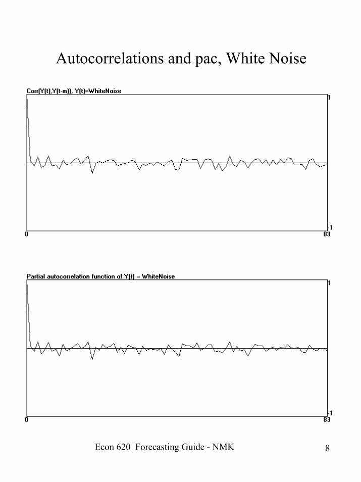
where εt is white noise. This givesa geometrically declining auto-correlation function (think of powersof α ) and a partial autocorrelation function with zeros for k>1 (why?)

MA(1): yt = εt + θεt -1

with εt white noise. The autocorrelationfunction is zero for k>1 and the pac function declines geometrically in absolute value but has positive valuesat odd lags (for θ positive) and negativevalues at even lags.

White noise has zero correlations of alltypes.

Econ 620 Forecasting Guide - NMK 6

White Noise

AR(1), parameter = 0.9

Econ 620 Forecasting Guide - NMK 7

MA(1), parameter = 0.9

Econ 620 Forecasting Guide - NMK 8

Autocorrelations and pac, White Noise

Econ 620 Forecasting Guide - NMK 9

Ac and pac for AR(1) (0.9)

Econ 620 Forecasting Guide - NMK 10

Ac and pac for MA(1) (0.9)

Econ 620 Forecasting Guide - NMK 11

These models can be extended to higherorder - AR(p) or MA(p). These givemore complicated patterns of auto-correlations. Also, the models can bemixed: ARMA models

For example: ARMA(1,1)

yt = αyt-1 + εt + θ εt -1

This can get out of hand -ARMA(p,q), ARIMA(p,d,q), etc.

Can get at stochastic seasonality withlagged variables - eg. In monthly data,we often use lags at 1,3, and 12, corres-ponding to monthly, quarterly, and annual dependence.

Econ 620 Forecasting Guide - NMK 12

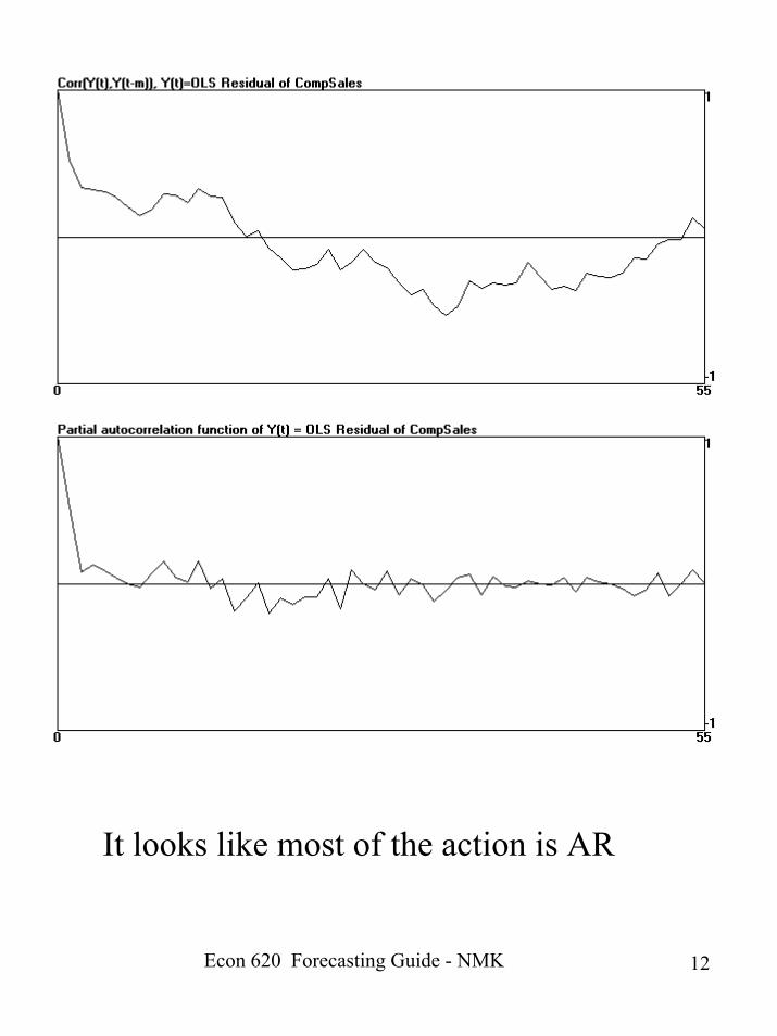
It looks like most of the action is AR

Econ 620 Forecasting Guide - NMK 13

An AR specification with lags at 1,2,3,and 12gives a better fit, with lag 2 insignificant

Econ 620 Forecasting Guide - NMK 14

The series is still quite volatile - we now dropthe lag at length 2 and add the number of saturdays in the month as an explanatory variable.

The standard error is 3946$ (compare withthe mean of 129552$) and the R-squared is0.88.

Econ 620 Forecasting Guide - NMK 15

The residual autocorrelation and pac functions are pretty flat ...

Econ 620 Forecasting Guide - NMK 16

As a check on the specification, a model(ARMA) with lags at 1,3, and 12 was fit to the residuals. None of the coefficientswere important and they were jointly insignificant, indicating that there is not much discernable structure remaining.

The forecast for 2000.11 is 130656$ with a standard error of about 4000$.

Econ 620 Forecasting Guide - NMK 17

Series 2: Transaction Counts- negative trend- clear seasonality

Econ 620 Forecasting Guide - NMK 18

Autocorrelation and pac functions (for the residuals from last slide)-looks like AR dominates again

Econ 620 Forecasting Guide - NMK 19

An AR(12) model shows important dynamics at lags 1, 3 and 12. Includingthe number of saturdays as well the results are:

Econ 620 Forecasting Guide - NMK 20

The residual autocorrelation and pacfunctions show little remaining structure

The prediction for Nov. is 29865, se 1032

Econ 620 Forecasting Guide - NMK 21

Sales Forecasts

Forecasts

100000120000140000160000

1/1/00

1/3/00

1/5/00

1/7/00

1/9/00

forecastactual

Econ 620 Forecasting Guide - NMK 22

Comp Store TCs

2000025000300003500040000

1/1/00

1/3/00

1/5/00

1/7/00

1/9/00

ForecastActual